A Sentinel-2 machine learning dataset for tree species classification in Germany

We present a machine learning dataset for tree species classification in Sentinel-2 satellite image time series of bottom-of-atmosphere reflectance. It is geared towards training classifiers but is less suitable for validating the resulting maps. The dataset is based on the German National Forest Inventory of 2012 as well as analysis-ready satellite imagery computed using the Framework for Operational Radiometric Correction for Environmental monitoring (FORCE) processing pipeline. From the National Forest Inventory data, we extracted the tree positions, filtered 387 775 trees in the upper canopy layer, and automatically extracted the corresponding bottom-of-atmosphere reflectance time series from Sentinel-2 L2A images. These time series are labeled with the corresponding tree species, which allows pixel-wise classification tasks. Furthermore, we provide auxiliary information such as the approximate tree position, the year of possible disturbance events, or the diameter at breast height. Temporally, the dataset spans the years from July 2015 to the end of October 2022, with approx. 75.3 million data points for trees of 48 species and 3 species groups as well as 13.8 million observations for non-tree backgrounds. Spatially, it covers the whole of Germany. The dataset is available at the following DOI (Freudenberg et al., 2024): https://doi.org/10.3220/DATA20240402122351-0.

1 Introduction

Climate change increases the risk of severe weather events such as heavy rainfall or drought in central Europe (Toreti et al., 2023). The recent past has seen large-scale forest diebacks due to drought, disease, insect infestations, or a combination of these disturbances (Senf et al., 2020; Senf and Seidl, 2021b). Forest managers face the challenge of adapting their management practices through diversification and other strategies to mitigate these threats. Here, remote sensing will play an increasingly important role as it can support well-informed decisions by providing extensive land cover and forest information at higher temporal frequencies than ground-based forest monitoring approaches. In this context, information on tree species is essential for many forest management decisions.

Tree species classification in satellite imagery is important, not only for scientific applications, but also for practical applications in forestry and nature conservation. This task has been a focus since the early days of spaceborne remote sensing with the first Landsat sensors (Walsh, 1980), and it continues today with the application of machine learning methods to large areas (Bolyn et al., 2022; Blickensdörfer et al., 2024).

Sentinel-2 (S2) satellite images are the ideal basis for such analyses, as they are standardized, freely available, and collected with high temporal revisit frequency. Machine learning, particularly deep learning, is commonly employed to tackle classification tasks in image data, although it requires substantial amounts of training data (Bolyn et al., 2022; Lake et al., 2022; Yuan and Lin, 2020). Deep learning is a type of machine learning that uses neural networks with multiple layers to automatically learn patterns from large datasets (Goodfellow et al., 2016). In the context of tree species classification, generating training data is demanding, and one has to resort to visual interpretation and on-screen labeling of high-resolution aerial images, ideally combined with validation in the field – or one has to source labels from forest inventory data.

Ahlswede et al. (2023) addressed the problem of training data compilation and created a multimodal training dataset containing aerial as well as Sentinel-1 and Sentinel-2 images of over 50 000 sites in the state of Lower Saxony, Germany. The dataset contains image-wise labels for 20 European tree species, generated from stand level forest inventory data. Utilizing different deep-learning models, the authors achieved an F₁ score of 54.6 % using Sentinel-2 data alone. The F₁ score is the harmonic mean of user's and producer's accuracy, or precision and recall, respectively. They concluded that “the integration of multi-seasonal data might disentangle further species-related information regarding phenology phases” (Ahlswede et al., 2023, p. 691) – this is what we aim for with the dataset presented here.

Hemmerling et al. (2021) used exactly these kinds of multi-seasonal Sentinel-2 data to classify 17 different tree species in the state of Brandenburg, Germany. They applied a random forest classifier to time series of the years 2018 and 2019 and reached F₁ scores between 67 % and 99 % for the nine most frequent species, thereby demonstrating that at least a subset of the species can be separated using S2 time series comparable to the ones provided here. As in the first study, the authors obtained their labels from forest inventories compiled by state authorities.

These two studies are noteworthy exceptions regarding the amount of training data used, because the used datasets were relatively large. Fassnacht et al. (2016) reviewed studies on tree species classification from remotely sensed data and concluded that “investigations focusing on […] a single often comparably small test site by far dominated the reviewed studies”. This hinders the generalizability of results and the applicability of generated models to other areas: a dataset covering a large area and long time spans is needed.

To overcome the problem of limited training data, we tap into the largest dataset of field observations of tree species in Germany: the National Forest Inventory (NFI). The German NFI runs in a cycle of 10 years, with a subsample after 5 years, and covers more than 25 000 sites, over 60 000 sampling points, and more than 500 000 trees across all ownerships and site conditions (Polley et al., 2018). For each tree, several variables such as species, relative position, and diameter at breast height (DBH, 1.3 m) are recorded. The resulting dataset is the most comprehensive available for German forests, and the derived statistics provide valuable insights into forest condition, composition, and development at the regional and national levels. However, the design of the NFI was not tailored to creating remote sensing reference datasets but to providing an efficient sampling and plot design for estimating key forest variables. From a remote sensing perspective, one of the major caveats is that the exact sampling positions need to be kept confidential, e.g., to prevent biased estimates when management practices are changed in the vicinity of the plot.

The goal of the work presented is twofold: first to make satellite data at NFI plot positions available to third parties without revealing the exact geolocations, and second to analyze the separability and temporal patterns of tree crown reflectances for tree species in Germany. We link NFI records to bottom-of-atmosphere (BOA) reflectance time series from matching Sentinel-2 images, enabling tree species classification and other applications for a broad range of potential users. Said time series were extracted from analysis-ready data generated by the Framework for Operational Radiometric Correction for Environmental monitoring (FORCE) (Frantz, 2019) hosted on the CODE-DE (https://code-de.org, last access: 22 January 2025) platform. The resulting dataset provides BOA reflectances from July 2015 to October 2022 and in total contains the time series of 387 775 individual trees and 70 242 non-tree locations. Multiplying the counts of tree and non-tree locations by their individual numbers of observed time steps yields a total of ca. 75.3 million data points for trees and 13.8 million observations for non-tree backgrounds, covering the entirety of Germany, 48 tree species, and 3 species groups. The primary purpose of the data is to train classifiers to detect tree species in satellite images from the Sentinel-2 mission, but they could also be used for studying phenological and spectral patterns of tree species. They are less suitable for validating maps at the pixel level. The dataset is available online at https://doi.org/10.3220/DATA20240402122351-0 (Freudenberg et al., 2024) with the CC BY 4.0 license.

2 Materials and methods

2.1 Study area and National Forest Inventory

The dataset covers the entire area of Germany, including its islands. More specifically, the dataset contains 24 925 of the 25 382 cluster plots recorded in the National Forest Inventory 2012. Either the missing cluster plots contained only trees below the canopy layer, the field inventory was compiled in a non-standard way (e.g., with custom postprocessing of the coordinates), or the cluster plot coordinates were simply missing from the database we obtained. Temperate broadleaf and mixed forests prevail in most regions of the country. Coniferous forests, mainly consisting of Picea abies (Norway spruce), dominate at higher elevations, and forests with Pinus sylvestris (Scots pine) occur in the sandy soils of the northeastern part of the country. In 2022, about 32 % of Germany was covered by forest (Riedel et al., 2024). Heavy droughts and the following insect infestations in the years 2018–2022 resulted in a decline in growing stock in certain areas (Reinosch et al., 2024; Thonfeld et al., 2022; Holzwarth et al., 2023).

The German National Forest Inventory is conducted on a regular, square sampling grid as shown in Fig. 1 with a grid size of 4 km × 4 km or less, depending on the federal state and region. At each grid point there are four inventory plots aligned in a 150 m × 150 m square. The southwestern corner of the square aligns with the grid, as shown in Fig. 2.

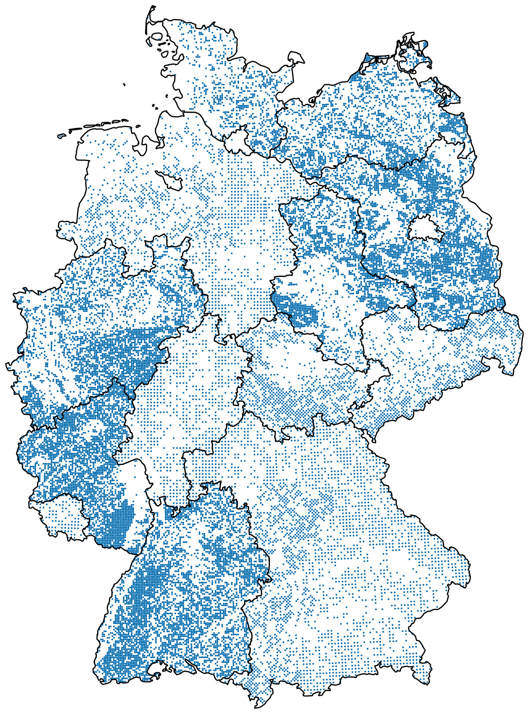
Figure 1 The sampling locations of the 2012 German National Forest Inventory. Borders: © GeoBasis-DE/BKG 2024.

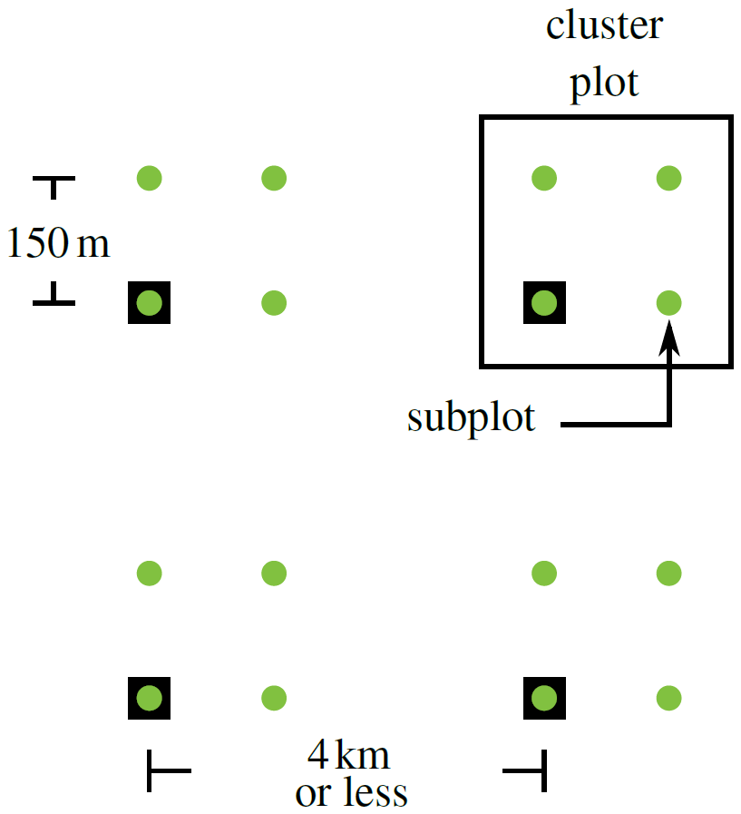
Figure 2 The German National Forest Inventory sampling grid (black squares) and the subplots (green). The southwestern subplot in each cluster plot is aligned with the overarching grid.

The geolocation of each subplot is measured with a Global Navigation Satellite System (GNSS) device, which may or may not be differentially corrected using correction information from terrestrial reference stations. At the subplot, two angle count samplings are performed (Gregoire and Valentine, 2007), which means that trees whose DBH covers more than a certain solid angle are recorded.

The first angle count sampling includes all trees within a distance from the sample location of 25 times their DBH (basal area factor 4). The positions of the selected trees are determined by measuring their azimuth angle using a compass and their distance to the plot center using an ultrasonic device (Haglöf Vertex or similar) or, in marginal cases, a measuring tape. Furthermore, the tree species, DBH, and other variables are recorded. In these measured tree positions, the BOA reflectances were extracted and related to the corresponding ground-measured information – how this was done is described later.

The second angle count sampling captures the surrounding forest composition by recording the species of all trees within a radius of 33.34 or 50 times their DBH (basal area factor 2 or 1), depending on how many trees were observed in the first sampling with basal area factor 4. The second angle count sampling allows one to say which subplots are pure stands, i.e., which have only one tree species. The information about stand purity is included in the dataset so that the user can filter for trees in pure stands.

2.2 NFI reference data selection

The reflectances recorded in a Sentinel-2 pixel represent the mixture of all land covers – or in our case tree species – within that pixel. However, in closed-canopy forests the BOA reflectance is dominated by the uppermost canopy layer, and we can safely assume that trees overshadowed by larger individuals contribute only little to the overall reflectance within a pixel. To compile the provided training dataset, we therefore filtered the NFI data for trees that are probably visible from above. We first removed all trees that grow in the understory; this information is recorded in the inventory. For the remaining trees, we modeled a circular growing space using the NFI's official method described in Riedel et al. (2017, p. 39, 40). The model establishes a species-specific linear relation between the basal area and the growing space of a tree. The growing space is a measure of the area occupied by a tree as a whole in an idealized forest stand. Lacking a model for direct estimation of crown area from basal area, we use the growing space as a proxy for it and stick to the term “crown area”. The model is defined in Eq. (A1), and the parameters are supplied in Table A1 in the Appendix. As we know the position of each tree as well as its predicted crown area, we removed trees that are probably not visible from above using a heuristic algorithm. We counted a tree as visible if it had the largest basal area of all trees within a radius of 3 m or its crown area was overlapped by surrounding trees by less than 50 %. Trees classified as visible by this heuristic formed the basis for the training dataset.

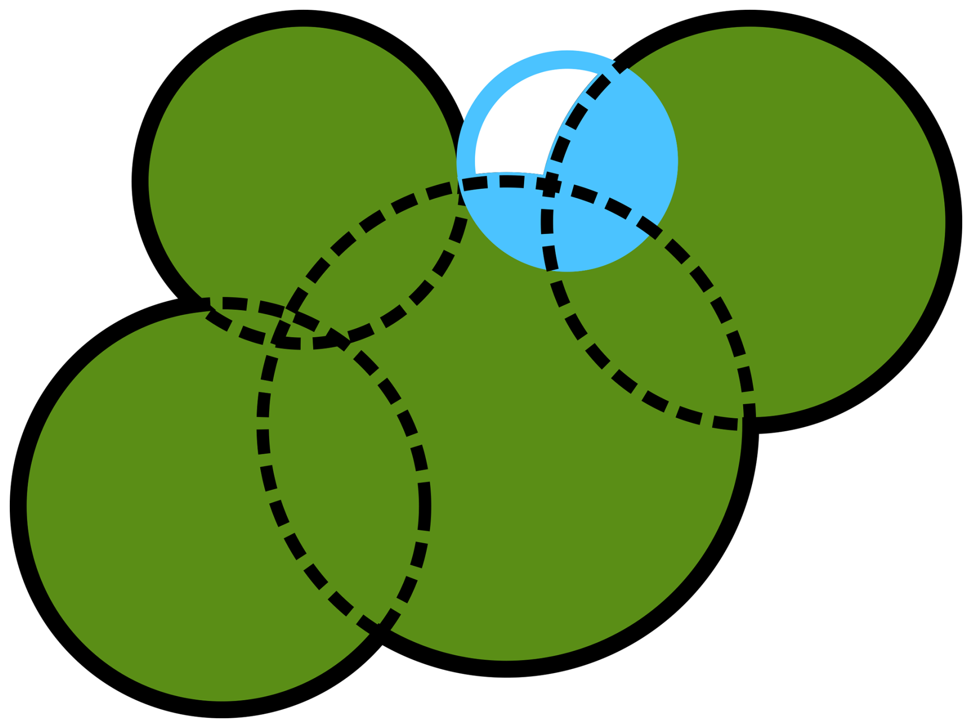
Figure 3 Sketch of a tree group: green trees are assumed to be visible. The blue tree area overlaps with other trees by more than 50 % and is therefore discarded.

To allow training of classification methods for discrimination between tree and non-tree pixels, we added non-forest observations to the dataset. For this, we sampled the tree cover density layer provided by the Copernicus Land Monitoring Service for the year 2018 within a 300 m × 300 m patch around the NFI plots (https://land.copernicus.eu/en/products/high-resolution-layer-tree-cover-density, last access: 22 January 2025). The tree cover density layer is sampled at locations that are at least 20 m away from the next pixel with a tree density greater than 10 %.

2.3 Satellite data selection

We used images from the Sentinel-2 satellites, preprocessed to analysis-ready level, which includes atmospheric correction and cloud masking using the FORCE processing pipeline (Frantz, 2019). FORCE provides a way of computing harmonized time series that are spatially and spectrally well aligned, which is discussed in more detail later. The resulting data comprise all S2 bands with 10 or 20 m resolution, with the 20 m bands pan-sharpened (resampled) to 10 m resolution. Additionally, FORCE provides quality assurance information (QAI) that aids in filtering out undesirable image conditions such as clouds, snow, or high water vapor content. The data are hosted on the CODE-DE (https://code-de.org, last access: 22 January 2025) and EO-Lab (https://eo-lab.org, last access: 22 January 2025) platforms. End users have the option of either downloading the preprocessed data or reprocessing them using the same settings for generating the FORCE data cube in CODE-DE. The necessary parameter files are provided alongside the dataset.

2.4 Time series extraction and data processing

Previous studies have taken different approaches to linking forest field data to satellite images. Many work only with pure stands (e.g., Verhulst et al., 2024; Hościło and Lewandowska, 2019), while others assign plot-specific species compositions (e.g., Blickensdörfer et al., 2024). Some sample individual pixels within polygons (Hemmerling et al., 2021; Grabska-Szwagrzyk et al., 2024), cut out pixels covered by a fixed-area plot (Persson et al., 2018), or even calculate reflectances at the individual tree crown level (Plakman et al., 2020).

As the German NFI performs angle count sampling, it is not possible to determine exactly how much of a given area (e.g., a Sentinel-2 pixel) is covered by which tree species and adjacent land cover types. In such cases, there are mainly two approaches one can follow for relating field and satellite data, which we call “tree-centric” and “pixel-centric”. The tree-centric approach assigns the most probable reflectance value to individual tree crowns by directly extracting them from the satellite image. In contrast, the pixel-centric approach labels individual pixels with species information, e.g., a species composition derived from inventory data. We chose the tree-centric approach, as it accounts best for the response design of the angle count sampling. With angle count sampling, an assignment of species information to pixels is difficult because it does not provide a full census of all trees over a specifiable area.

We started by clipping 300 m × 300 m image patches containing the 24 925 filtered NFI cluster plots and their surroundings from the FORCE data cube, as depicted in Fig. 4. We extracted the BOA reflectance as well as the QAI. Before extraction, we filtered the plots to ensure that they contained at least one pixel with data not affected by clouds or cloud shadows.

Figure 4 The time series extraction workflow: first, 300 m × 300 m tiles are clipped from the FORCE data cube for Germany for all records between 2012 and 2022. Second, the pixel-wise time series are extracted from the tile time series.

In a second step, we extracted the BOA and QAI pixel time series from the patches in each tree position. In cases where a single tree covered more than one 10 m × 10 m Sentinel pixel, we calculated the area-weighted average of all pixels intersected by the tree's crown area, as depicted in Fig. 5. Each extracted satellite observation was then linked to its acquisition date, the corresponding NFI data, and more information. Senf and Seidl (2021a) provide a Landsat-based map of forest disturbances for Germany between 1986 and 2020 at a resolution of 30 m. To be able to identify possible disturbance events, we included the disturbance year from this map in the dataset. However, this still leaves a gap between 2020 and 2022 for which no disturbance information is available. This was bridged by attaching the information on whether the trees were still present in the 2022 NFI. To enable approximate spatial analyses, we furthermore included the center coordinate of the 1 km INSPIRE grid tile that the cluster plots are located in. The INSPIRE grids (INSPIRE MIG, 2023) are a set of pan-European geographical grid systems in the ETRS89-LAEA coordinate reference system with their origin at 52° N, 10° E. The grids have a spacing in meters, equaling a power of 10; we used the 1 km grid.

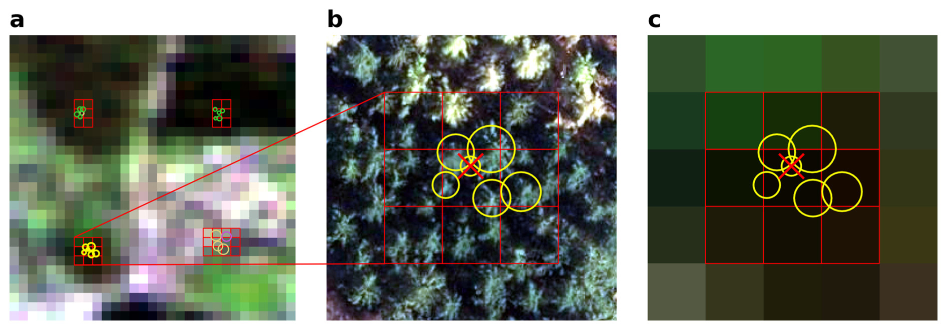
Figure 5 (a) The whole cluster plot cutout of 300 m × 300 m. S2 image: European Space Agency (2021). (b) The lower-left subplot with the corresponding orthophoto for reference. Douglas firs are in the lower part of the image, and Norway spruce is in the upper part of the image. Image: © BKG 2021. (c) The S2 pixels corresponding to the subplot, with the circles depicting the modeled tree crown areas. The crossed-out tree is omitted because it overlaps too much with the surrounding trees.

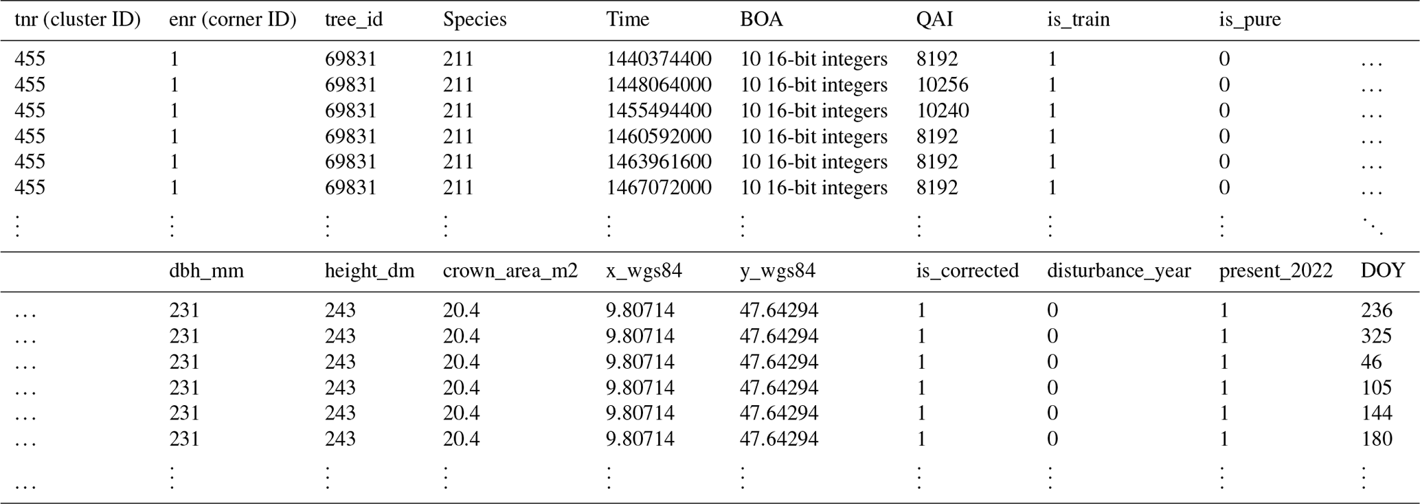
The final dataset comprises the columns presented in Table 1, and an excerpt is given in Table C1 in the Appendix. All samples were randomly split into training and validation sets based on their cluster plot IDs with a ratio of 70 %–30 %. This rules out any spatial overlap between the training and test sets and reduces correlations between the two. For benchmark studies, we recommend using this split to ensure comparability across publications.

Senf and Seidl (2021a)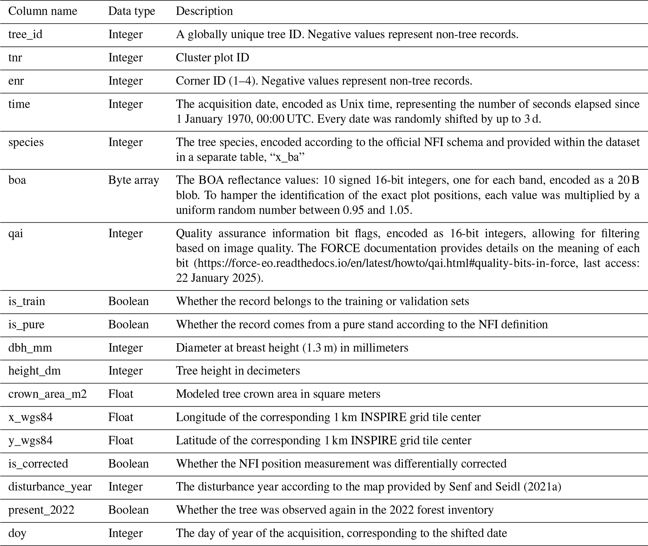

Table 1 Dataset contents and column descriptions.

2.5 Assessment of the geolocation accuracy of the NFI plots

The tree positions in the NFI are measured in polar coordinates relative to the plot center using a compass for the angle and an ultrasonic device for the distance measurement. We assume that the errors for angle and distance are small compared to the GNSS error of the plot center position measurement. GNSS measurements can be differentially corrected by using ground-based reference stations to increase the positional accuracy. Depending on the federal state and field team, coordinates of the plot centers are measured with corrected GNSS devices or not. Of the subplots with trees in the dataset, 76.5 % were corrected, 22.5 % were not, and the remainder have an unknown status.

To estimate the accuracy of the plot center coordinates, we compared the field-measured tree positions with tree positions derived from true-ortho aerial images obtained from the Federal Agency for Cartography and Geodesy. These images are orthorectified using a surface model and aligned with high accuracy to ground control points. The ATKIS orthophoto standard guarantees a geolocation error with a standard deviation of 0.4 m or less (Arbeitsgemeinschaft der Vermessungsverwaltungen der Länder der Bundesrepublik Deutschland (AdV), 2020). Two expert image interpreters then manually shifted a sample of 200 NFI plot positions, and thereby the trees, to match the true tree positions by comparing local tree patterns as depicted in Fig. 6. This allows us to quantitatively evaluate the deviation of measured positions from true positions and to compare the accuracy of corrected and uncorrected measurements.

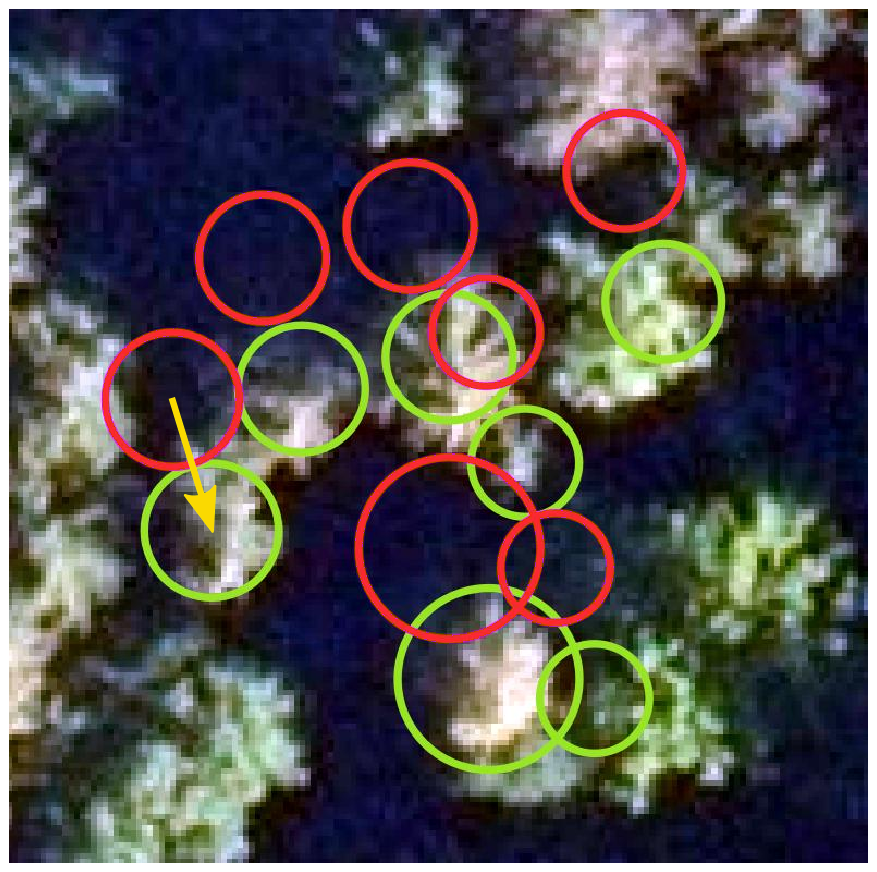
Figure 6 Original measured GNSS coordinates (red) were shifted (here by 4.8 m) to the visually best-matching position (green) in aerial orthophotos to quantify GNSS errors. The circles depict modeled crown areas. Image: © GeoBasis-DE/BKG 2024.

2.6 Species separability analysis

To detect inconsistencies within the dataset, we computed the infrared reflectance histograms of five species for mixed and pure stands. If the histogram shows artifacts like double peaks or differs strongly between pure and mixed stands, this could indicate deficiencies in the respective parts of the dataset. The histograms were computed for band B8 (842 nm), averaged over all records in June 2021 for a sample of five species whose occurrences are correlated – Betula pendula often grows along with Pinus sylvestris, and Fagus sylvatica often appears together with Quercus spp. June 2021 was chosen because both Sentinel satellites were operational and, unlike the preceding years and 2022, 2021 was not particularly dry.

3 Dataset description and statistics

3.1 Numerical species distribution

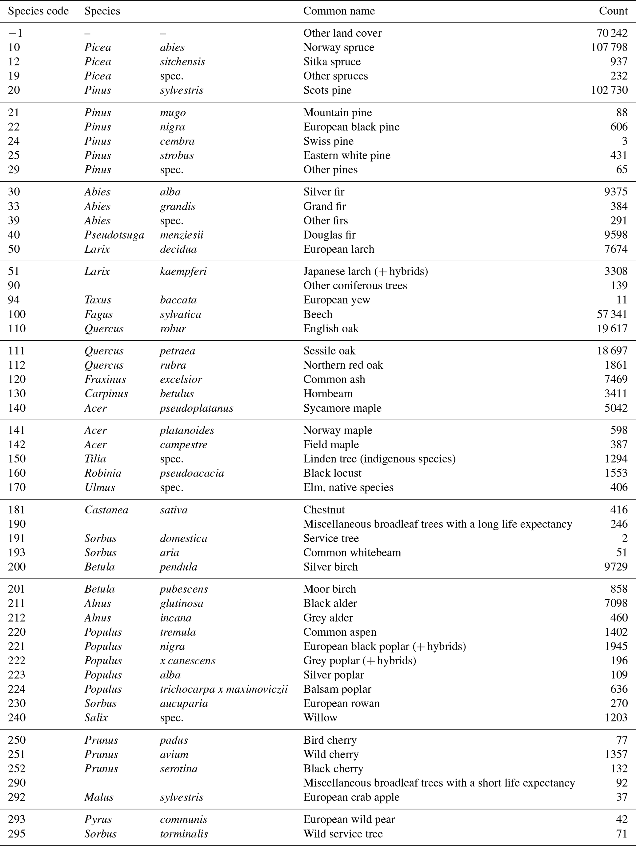
Due to the greatly varying dominance of tree species in Germany, the numerical distribution of the different species (Fig. 7) is heavily imbalanced. The most abundant species is Pinus sylvestris (Scots pine), followed by Picea abies (Norway spruce), Fagus sylvatica (European beech), and the different Quercus (oak) species. A complete list of the included tree species and their counts can be found in Table C2.

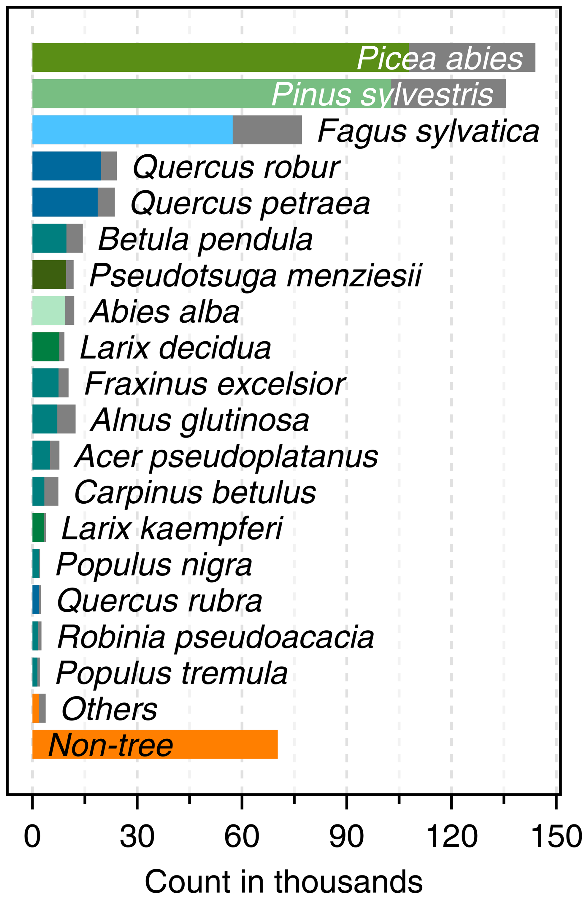
Figure 7 The numerical species distribution in the training dataset (colored) and in the original NFI 2012 data (grey).

3.2 Temporal signatures of selected species

Evergreen and deciduous trees can be clearly separated visually by inspecting the time series of their infrared (IR) reflectance, as depicted in Fig. 8. In the presented time series, the observations for a given species and point in time have been averaged across all undisturbed individuals in pure stands. Whether a stand is pure or not was determined using the second angle count sampling of the NFI (basal area factor of 1 or 2). Obviously, deciduous broadleaf trees exhibit a much stronger seasonal pattern than evergreen coniferous trees in our dataset. This separation is less evident in the green band, likely due to its higher susceptibility to atmospheric effects and its lower absolute reflectance, which combine to diminish the signal-to-noise ratio. While the temporal infrared profiles of Fagus sylvatica and Quercus robur are generally distinguishable across most years, there are instances where differentiation becomes challenging (e.g., 2016 and 2020). Quercus robur tends to have a slightly lower IR reflectance on average, particularly in summer. Picea abies and Pinus sylvestris also differ only slightly in the infrared, with Picea abies trending towards having lower average values. Overall, differentiating species by their temporal profiles alone seems challenging without considering their spectrum at the same time. Figure B1 in the Appendix depicts the same data as Fig. 8 but additionally includes error bands that were omitted here for clarity.

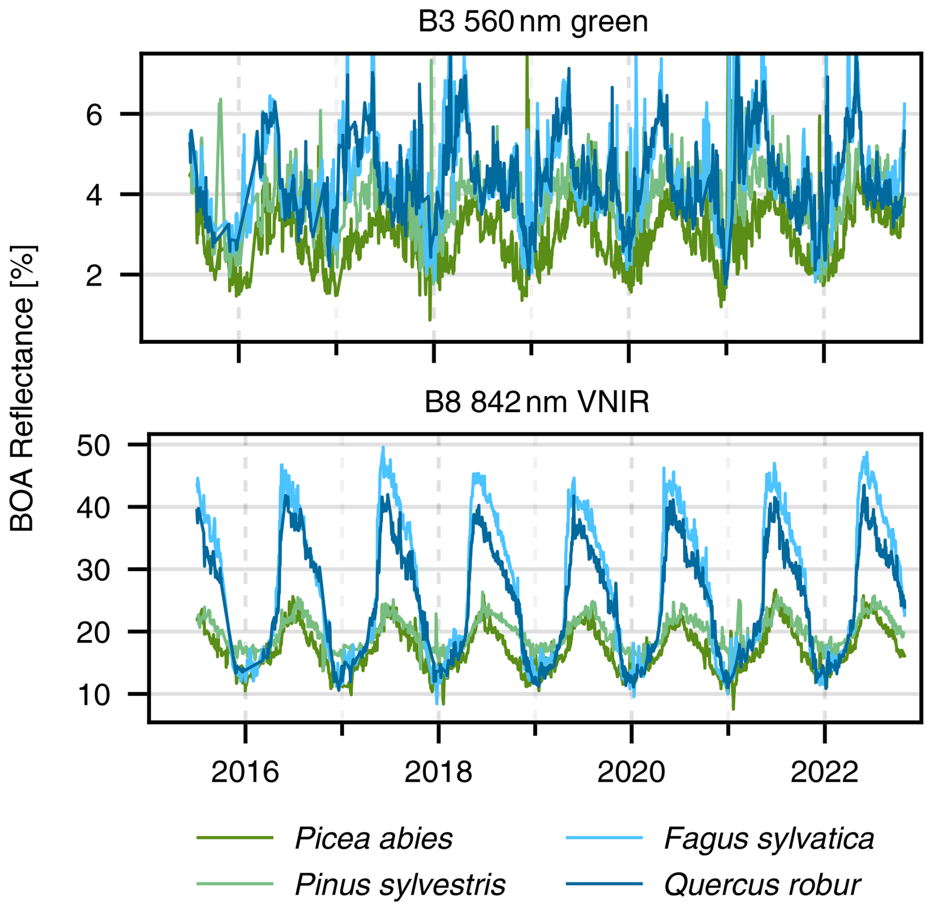
Figure 8 Time series of BOA reflectance for the indicated species, averaged over all undisturbed individual trees in pure stands at a given time. The data have been filtered to exclude all types of cloud cover as well as their shadows, snow, and pixels with high aerosol optical depth.

Looking at a random selection of four individual trees' time series, depicted in Fig. 9, it becomes clear that, at the level of a single tree, the differences between species still seem to be present but with high variance from year to year.

Figure 9 Time series of random single trees of different species.

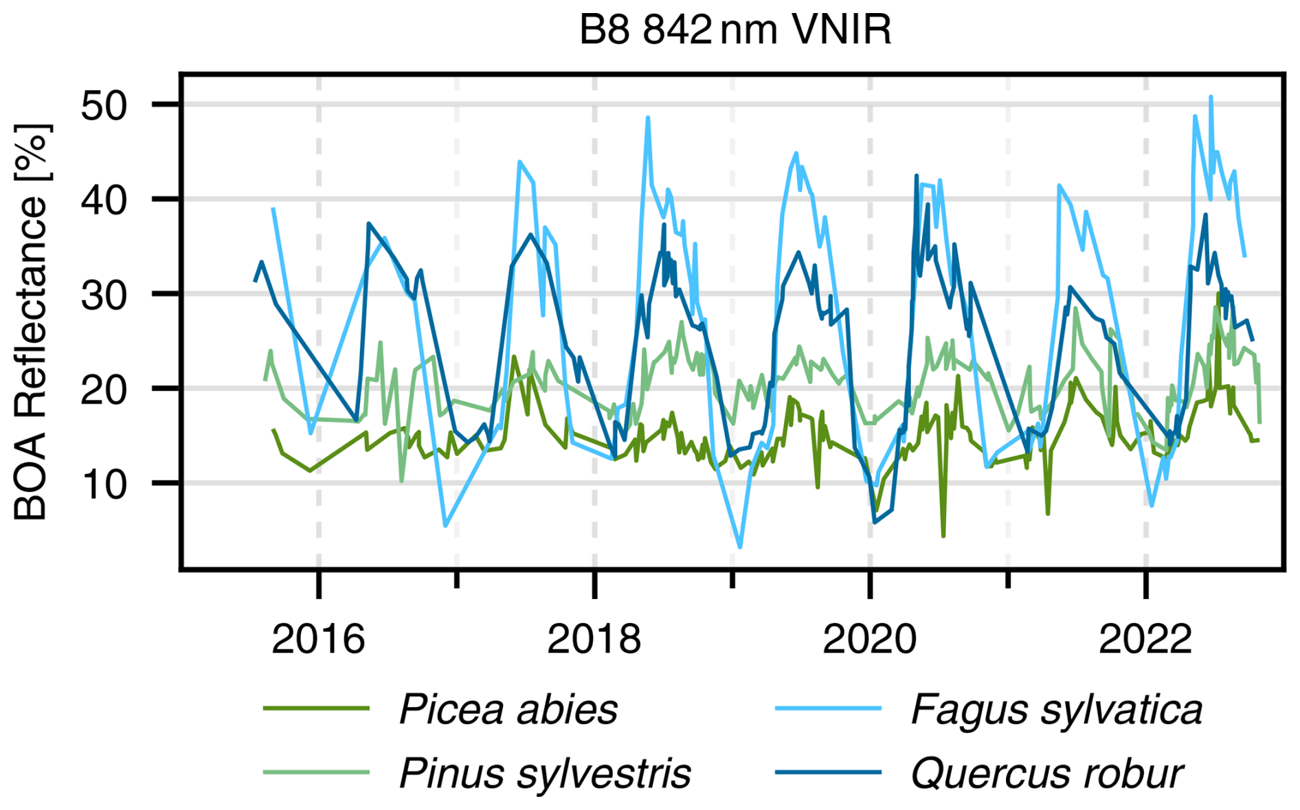
Figure 10 shows the total observation count over time, i.e., how often each tree was imaged in a month, summed up across all the trees. After the commissioning of Sentinel-2B in June 2017, the number of observations increased. As one would expect, there are more observations in the summer months when clouds are less likely, and especially from 2018 onward the counts regularly reach over 1 million.

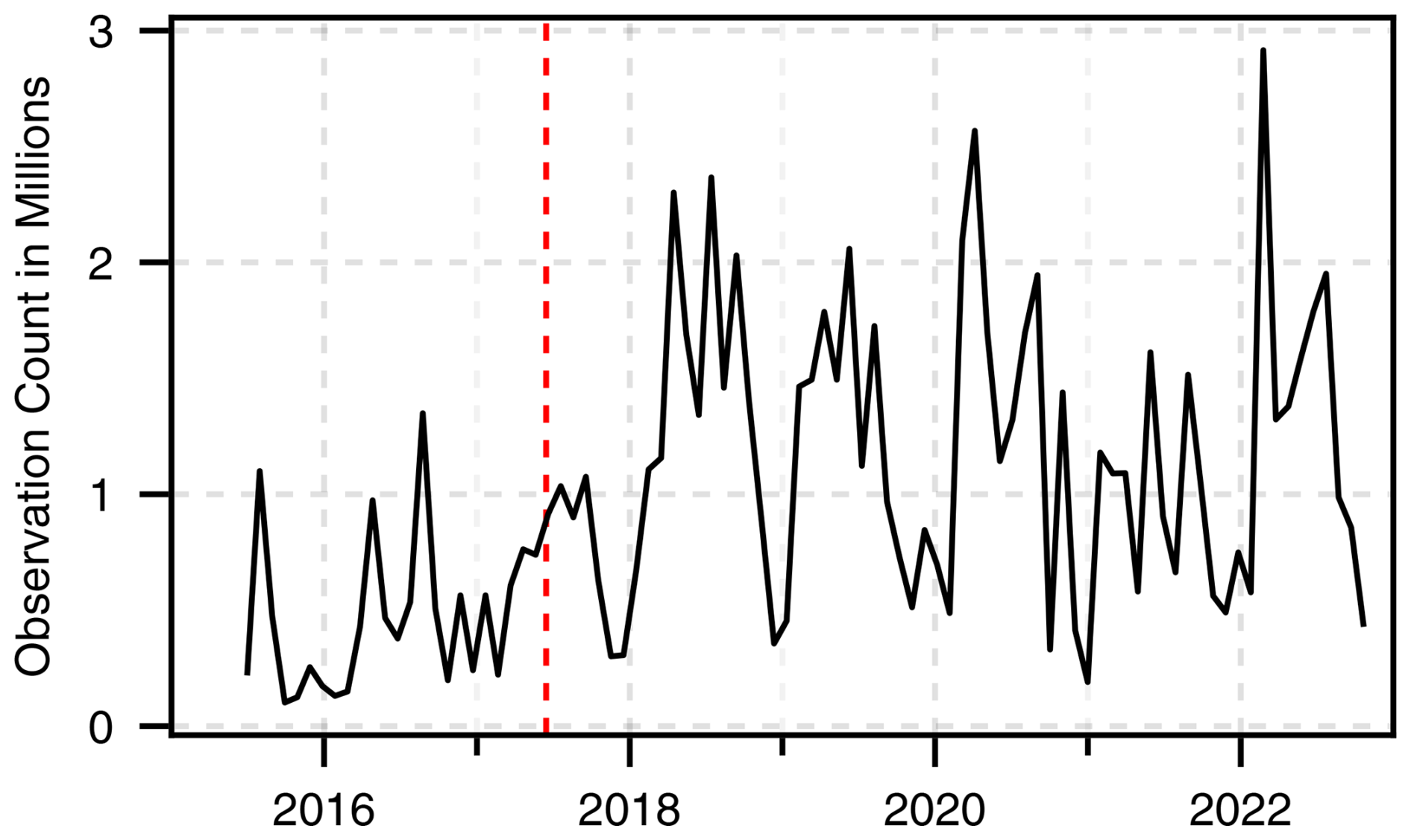
Figure 10 Total monthly observations of all trees in the dataset (tree count multiplied by individual observation count per month). The vertical red line corresponds to the Sentinel-2B commissioning date.

3.3 Spectral signatures

Besides the temporal variation of the reflectance, the spectral variation is an important feature for the tree species classification – however, the species are not necessarily separable by their spectra alone, as can be seen in Fig. 11. It depicts the Sentinel-2 spectra of the five most frequent species as well as the background classes. Fagus sylvatica and Quercus petraea, for example, have almost matching spectra, especially at the shorter wavelengths. The resulting spectra match the ones presented in Immitzer et al. (2016).

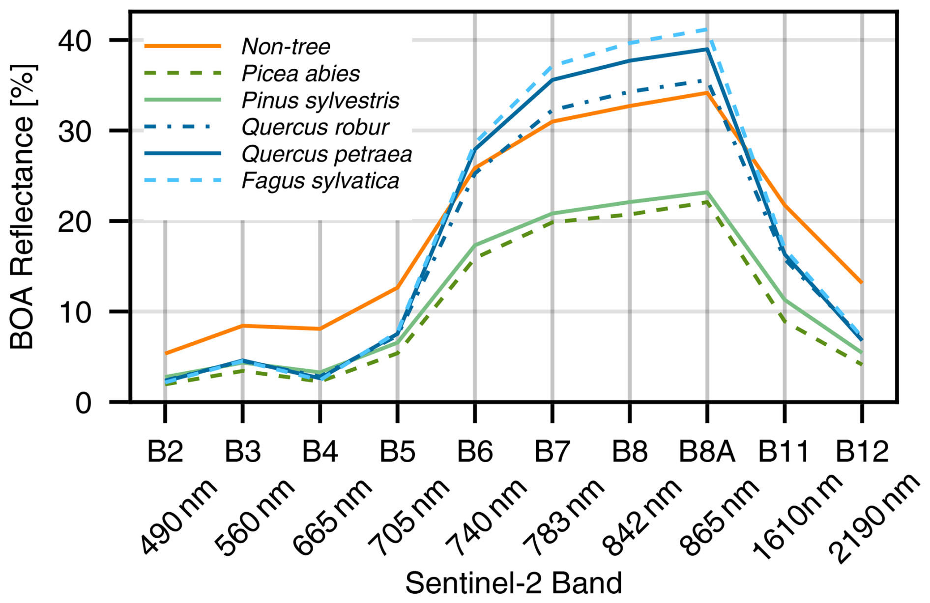
Figure 11 Average spectrum of the five most frequent species in the dataset plus the background class. Records from pure stands have been averaged between May and August (inclusive) of the years 2017–2022.

3.4 Spatial distribution

It can be expected that the temporal signatures will vary with local conditions, e.g., along a latitudinal or elevation gradient. Therefore, it is important to analyze the spatial coverage of the training data. Figure 12 shows that Picea abies (a) is mainly present in the southwest of Germany and in the lower mountain ranges. Pinus sylvestris (b), on the other hand, is predominant in the sandy soils of the northeastern part of the country. The different Quercus species (c) mostly occur in the west of Germany but are also present throughout the rest of the country. Fagus sylvatica (d), lastly, co-occurs with Quercus spp., but in contrast to them manages to settle in the higher and therefore colder hillscapes of the central parts of Germany. Note however that these spatial distributions are derived from the dataset, which does not mirror the NFI one to one due to filtering and the availability of satellite images.

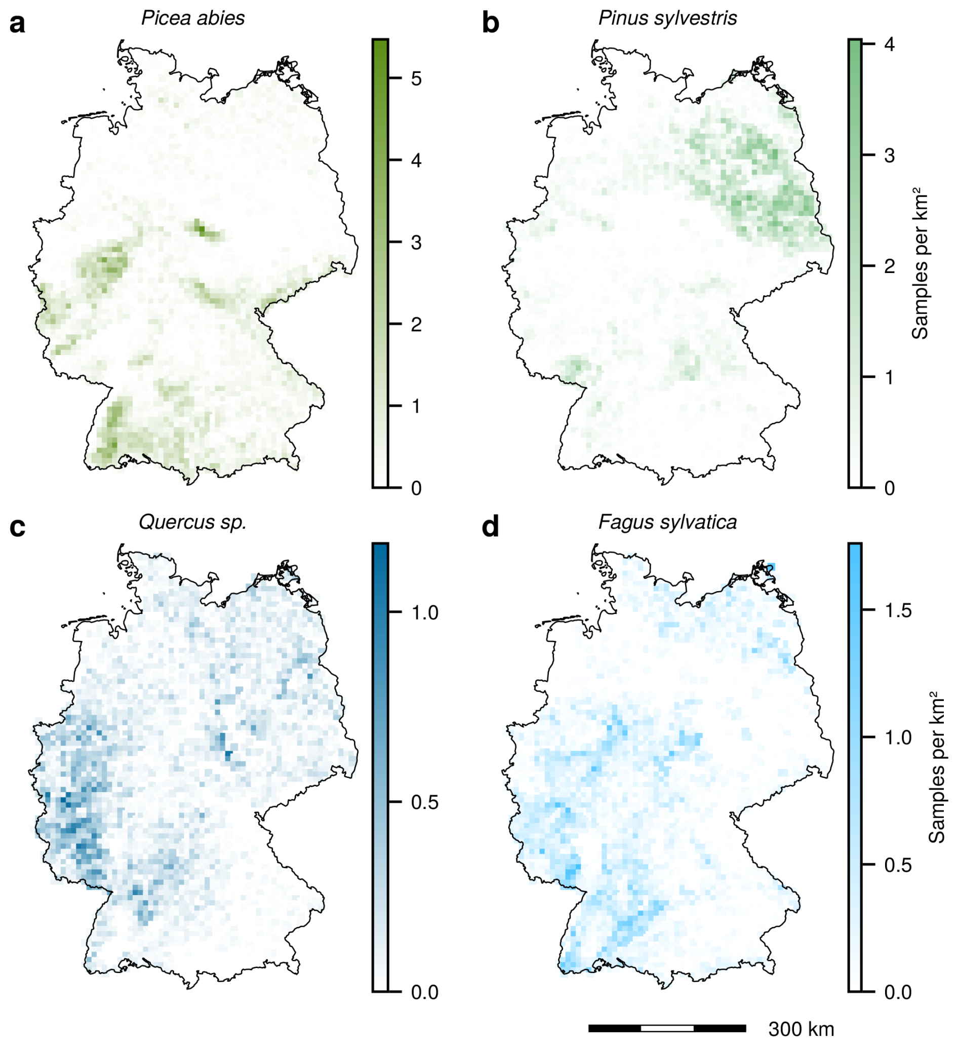
Figure 12 Spatial tree distribution of tree density for different species. Note the different scales. Borders: © GeoBasis-DE/BKG 2024.

3.5 NFI geolocation accuracy estimation

The analysis of the spatial accuracy of the NFI plot coordinate GNSS measurements reveals that 95 % of the corrected GNSS positions deviated by less than 11.2 m and 81 % by less than 5 m. Figure 13 depicts the corresponding histogram along with the empirical cumulative density function. Against expectations, the comparison of corrected and uncorrected GNSS measurements shows no significant difference.

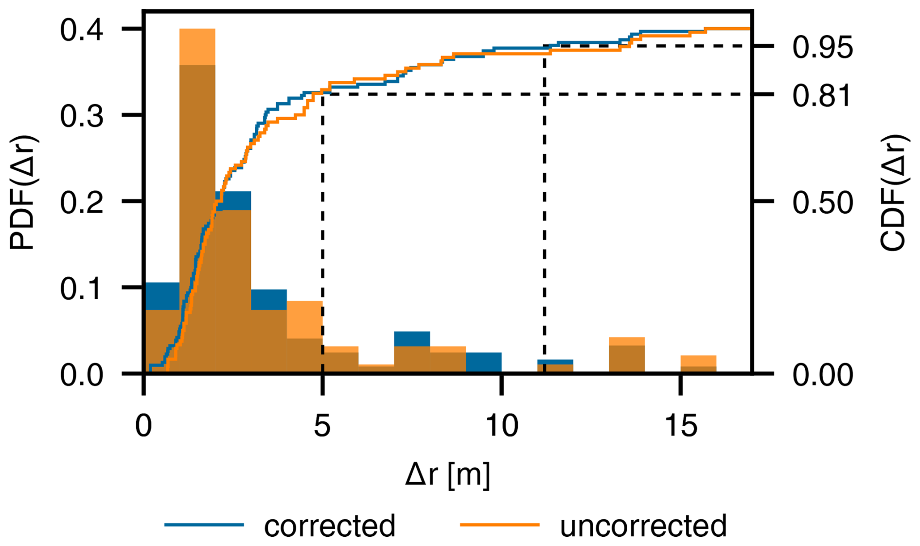
Figure 13 Histogram of the distances by which the plot locations were shifted from the original GNSS positions. Differentially corrected measurements are depicted in blue.

3.6 Separability analysis

Figure 14 shows the histograms of S2 band B8 (842 nm), averaged over all records in June 2021 for the species pairs Betula pendula–Pinus sylvestris and Fagus sylvatica–Quercus robur–Quercus petraea, each computed over mixed and pure stands, respectively. These combinations were chosen because the respective species often co-occur. The reflectance distributions for Pinus and Betula clearly differ between mixed and pure stands. In mixed stands, the distributions are relatively wide and overlap, whereas in pure stands there are separable peaks (although some overlap remains) and the distance between the maxima is larger. Comparing Fagus sylvatica to the two Quercus species, one can see that the distributions overlap much more, as all three species are broadleaved. In mixed stands, there is hardly any observable difference between the distributions. In pure stands, the distributions still overlap significantly, but the distance between peaks is slightly greater than in mixed stands.

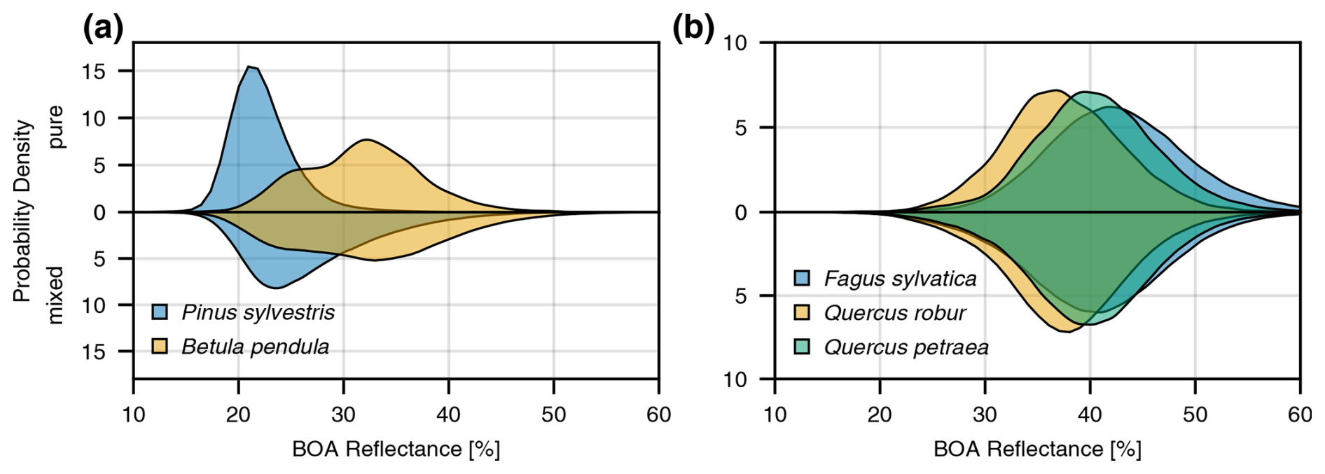
Figure 14 Histogram of near-infrared (842 nm) BOA reflectances, averaged over all trees in June 2021 for (a) Pinus sylvestris and Betula pendula and for (b) Fagus sylvatica, Quercus robur, and Quercus petraea. The upper parts represent pure stands and the lower parts mixed stands.

4 Discussion

4.1 Geolocation accuracy

For Sentinel-2, to obtain the presented dataset, we linked spatial information from two different data sources: georeferenced satellite images and on-ground GNSS measurements. A misalignment of these sources might lead to extraction of wrong pixel values from the image data. FORCE co-registers all Sentinel-2 images with averaged Landsat time series. The Landsat images are in turn co-registered with the Sentinel-2 global reference image, which results in a geometric accuracy of 10.2 m at the 90 % confidence level for Landsat 8 (Haque et al., 2022) (8 m at 80 % confidence). Consequently, this is the best estimate for the spatial accuracy of the S2 images used. The reason for this cyclic co-registration of Sentinel to Landsat to Sentinel is that so far only the S2 level-1 archive has been processed to a common standard (https://sentinels.copernicus.eu/web/sentinel/technical-guides/sentinel-2-msi/copernicus-sentinel-2-collection-1-availability-status, last access: 22 January 2025). The level-2 data, which compensate for atmospheric effects and are needed for coherent time series, are not yet available on a standardized processing baseline in any public archive.

For NFI geolocation accuracy, the comparison of corrected and uncorrected GNSS measurements showed no significant difference in spatial accuracy, at least not in the way we measured it. As differential correction unquestionably increases GNSS accuracy, we suppose that increasing the count of sampled plots as well as the number of image interpreters would change our result. Furthermore, trees growing skew and outliers matching the crown patterns might have influenced the results negatively. Lastly, it will be interesting to analyze the accuracy of trained classifiers as a function of correction status.

Combined geolocation accuracy is difficult to compute for several reasons: (1) the satellite images are corrected by FORCE, as discussed above; (2) the satellite image accuracy is latitude- and time-dependent (S2 Data Quality Reports: https://sentiwiki.copernicus.eu/web/document-library, last access: 22 January 2025); and (3) the GNSS errors we measured do not follow a Gaussian distribution. Neglecting these points and using the values derived for the 80 % confidence level, i.e., 8 m for the satellite images and 5 m for the GNSS positions, we obtain an error estimate of 9.4 m. This is nearly equivalent to the pixel size, which means that the extracted pixel values are still likely to represent a reasonable approximation of the targeted trees, whose diameter is of a comparable size. Lastly, the error of 9.4 m is likely overestimated for two reasons: first, the true error distributions of GNSS and satellite geolocation error magnitudes is lognormal (as opposed to a Rayleigh distribution), typically with a higher share of small magnitudes. Second, the 8 m satellite geolocation error is derived for a single Sentinel-2 scene but is averaged out by the co-registration process.

4.2 Adverse imaging conditions

During the extraction process, we filtered out most pixels with cloud cover or cloud shadows. FORCE employs the FMASK algorithm (Zhu and Woodcock, 2012) for cloud detection, which has an accuracy of 84 % for cloud or clear detection and a 72 % detection accuracy for cloud shadows (Aybar et al., 2022). Consequently, falsely labeled image regions lead to commission or omission errors in the final dataset; i.e., usable pixels might be removed by being labeled as cloudy, or cloud pixels could be in the dataset. However, there are other imaging conditions that might affect the quality of a pixel, like high aerosol content, snow, or poor illumination conditions. FORCE encodes this information in the quality assurance information, and end users can use this to further narrow the dataset down to only the highest-quality pixels.

4.3 Extraction of non-forest points

The non-forest points were randomly sampled within the extracted 300 m × 300 m tiles. In consequence, we only sampled non-forest points from areas like city centers or industrial zones where they are situated close to forests – which is rather unlikely. Therefore, the extracted non-forest points are biased towards rural villages and agricultural areas.

4.4 Taxonomic identification

The field teams of the NFI data are trained and undergo testing before being allowed to take samples. However, it cannot be ruled out that, under adverse conditions, certain species are confused. We cannot quantify this error but assume that the vast majority of tree species identifications are correct, in particular for common species.

4.5 Tree-centric pixel extraction

As described in Sect. 2.4, there are different ways of linking satellite image data to field information. We took a tree-centric approach and extracted reflectances for every tree in the dataset. Compared to the pixel-centric approach, this comes with advantages and disadvantages. The main advantages of the tree-centric approach are that it reflects the response design of angle count sampling and one obtains the best estimate for the spectral reflectance of a given tree crown. This also allows one to extract data for rare species and those that only appear in mixed stands, although their statistics will be influenced by mixed pixels. Lastly, one does not need to define a dominant species based on arbitrary thresholds, as was done in Persson et al. (2018), for example.

A drawback in comparison to the pixel-centric approach is that different tree crowns can receive the same spectral signature. For example, if two tree crowns are completely located within the same S2 pixel, they receive identical values and information is duplicated. We checked the non-randomized dataset for duplicate bottom-of-atmosphere reflectances among the tree records. Non-tree points were sampled from a larger area, so duplication plays no role in their case. To identify duplicates, we grouped the dataset by cluster ID, corner ID, time, and reflectance spectrum. If there were N identical reflectances per group, we counted N−1 as duplicates. In total, the dataset subset for trees contains ca. 4.87 million duplicate entries out of ca. 66 million, which translates into 7.38 %. Out of these 4.87 million duplicates, 3.86 million (5.84 %) are duplicates with identical species labels and 1.01 million (1.53 %) have differing species labels. Ergo, at least 0.77 % (1.01 million of 66 million $/$ 2) of the labels are wrong.

Should the user wish to reduce the correlation between samples or remove duplicate pixel time series, we recommend the following procedure: first, group the dataset by subplot; second, compute the correlation of the full time series between the different trees in the plot; and finally, remove all trees that correlate beyond a certain threshold, except for one.

A weakness that both approaches, tree-centric and pixel-centric, share is mixed pixels: at present, we cannot exactly quantify the effect on our dataset of pixels that contain different tree species, as it is in most cases impossible to derive the species shares of a pixel based on the NFI data. The NFI does not fully sample a given plot, so in most cases labels are only available for parts of a given pixel. Another source of mixed pixels are the 20 m resolution bands of Sentinel-2 that are pan-sharpened to 10 m by FORCE, thereby distributing identical information across several pixels.

4.6 Species separability analysis

Figure 14a shows that the IR–reflectance distributions of Pinus and Betula are wide and overlap in mixed stands, whereas they are more separated in pure stands. We interpret this as a potential indication that, at least for this species pair, the dataset may contain mislabeled data due to insufficient spatial accuracy or the extracted pixel values originate from mixed pixels containing other species or land cover classes.

In contrast, comparing Fagus and Quercus spp. in mixed and pure stands revealed no significant differences, with the reflectance distributions overlapping substantially. However, this does not necessarily indicate labeling errors; it could also reflect naturally occurring values. This highlights the necessity of including factors beyond spectral data, e.g., temporal profiles as shown in Fig. 9, for accurate species classification.

4.7 Considerations for map production

The purpose of this dataset is to train classifiers, ultimately for mapping of tree species. These classifiers will have a certain model accuracy derived from, e.g., the validation split of the presented dataset. However, caution is required when judging the accuracy of generated maps based on models – model accuracy should not be used as the sole basis for validation. This applies to the current dataset as well, since heuristic data filtering or pixel duplication may have altered the distribution of reflectance values in a way that could negatively affect the results. Users should also consider this when applying additional data filters, e.g., for the DBH. Consequently, we recommend auxiliary data for validating generated maps. If users wish to validate maps based on the presented dataset, they can do so using aggregate statistics, such as at the state level, since the dataset contains coarse location data that make it suitable for such analyses. However, such analyses will be restricted to trees that are visible from above according to our heuristic. Furthermore, areas covered by tree species, as derived from the maps produced, can be compared to population estimates from the NFI, which are publicly available (J.H. von Thünen-Institut, 2024). Lastly, the “area of applicability” approach developed by Meyer and Pebesma (2021) can be used to ensure that models are not applied outside the predictor variable space, thus preventing potential bias.

5 Data availability

All the data are available online at https://doi.org/10.3220/DATA20240402122351-0 (Freudenberg et al., 2024) with the CC BY 4.0 license.

6 Conclusion and outlook

In this work, we present the most comprehensive dataset so far of annotated Sentinel-2 time series data for tree species detection in Germany. With over 380 000 trees of 48 species observed for over seven years, this dataset can significantly advance research into automatic tree species classification for Germany and central Europe. At the same time, the described approach can serve as a pilot study for making NFI data from other countries accessible to the remote sensing community, e.g., for training machine learning models without releasing exact geolocations publicly. Lessons learned from its application can be used to enhance future inventories and datasets. For example, it could show that, for underrepresented species, more labels are required, and in turn they could be sampled in targeted inventories.

As discussed in the previous section, the dataset still has several shortcomings that could be improved. To achieve better agreement between labels and images, the spatial accuracy of the data sources has to be increased. To do so, we suggest that in future all NFI position measurements be taken using differential GNSS devices, although we saw no significant differences in accuracy. Furthermore, we expect that aligning the Sentinel-2 images directly with the S2 global reference image instead of averaged Landsat time series would improve their spatial accuracy and make it easier to derive interpretable error metrics. We consider releasing an updated dataset version as soon as the newly aligned Sentinel L2A collection is fully accessible.

The main focus of further efforts will be to increase the number of labels for weakly represented classes, e.g., by utilizing automatically classified high-resolution orthophotos as a reference. Our first attempts to automatically identify underrepresented tree species in standard RGBI aerial images with 20 cm spatial resolution have failed, so the presented dataset is still limited regarding less abundant species. Another option for increasing the overall amount of data would be to incorporate forest inventory data at the stand level from, e.g., state forest enterprises. However, these data often only provide estimates of tree species proportions within management units but no geolocation of individuals.

We hope that this dataset will foster research into time-series-based classification of tree species and believe that it offers many possibilities for analyses that go beyond the ones presented here. Users can freely recombine the provided data, calculate basal or crown area proportions per sampling location, and use this information as labels instead. Using classification methods in general, one could investigate which spectral bands and which points in time are crucial for precise species classification. As the dataset contains not only the time series of individual trees' BOA reflectances but also their approximate locations, spatiotemporal patterns in tree phenology could be assessed at the individual species level. For example, the onset of leaf emergence could be analyzed first in the dataset alone and later using species maps generated by a derived classification method. Lastly, the dataset could be used to correlate reflectances and approximate health conditions with meteorological events like droughts at a per-species level. This would open up further research into climate-change-resistant species and enable the identification of endangered forest stands. In the future we plan to release updated versions of the dataset, particularly after the final publication of the 2022 NFI.

Appendix A: Crown area estimation

The following equation is used to model the crown area with the parameters α and β from Table A1 (Riedel et al., 2017, p. 39, 40).

$$\begin{array}{}\text{(A1)}& A_{\mathrm{C}}=\mathit{\alpha }+\mathit{\beta }{A}_{\mathrm{B}}\end{array}$$

A_C is the tree crown area, and A_B is the basal area.

Table A1 Parameters of the crown area equation (Riedel et al., 2017, p. 40). We corrected the α value for poplar; the original value was 23, which is a typing error.

Appendix B: Additional figures

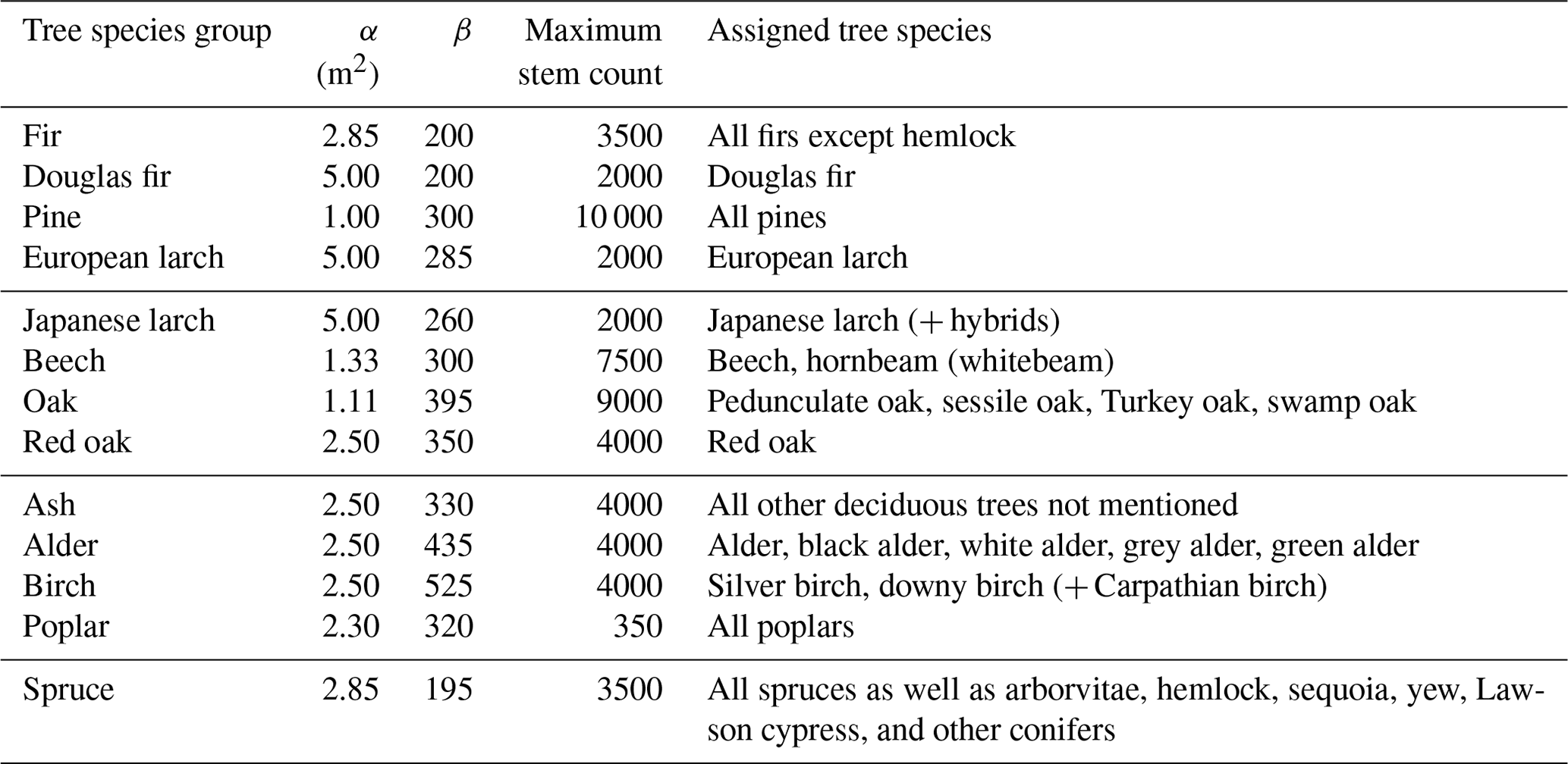
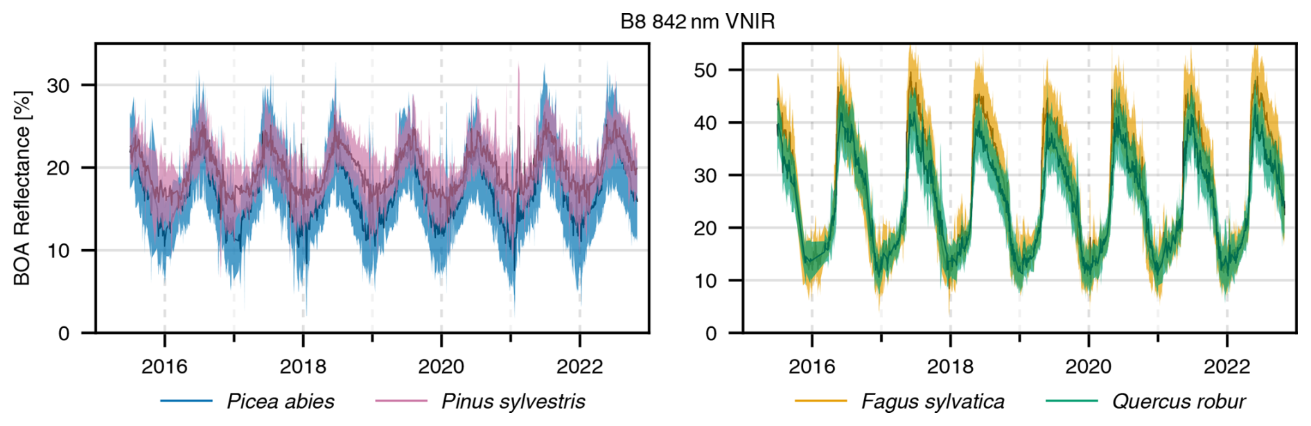
Figure B1 Time series of infrared reflectance and the standard deviation for the indicated species, averaged over all undisturbed individual trees in pure stands at a given time. The bands have a width of 2 standard deviations. The data have been filtered to exclude all types of cloud cover as well as their shadows, snow, and pixels with high aerosol optical depths.

Appendix C: Database excerpt and species counts

Table C1 Database excerpt. The bottom-of-atmosphere (BOA) reflectance is encoded as 10 signed 16-bit integers, and the quality assurance information (QAI) is a single 16-bit integer. DOY stands for “day of year.”

Table C2 List of all the included tree species with counts.