Global agricultural lands in the year 2015

While there are many global geospatial datasets representing the extent of agriculture, they predominantly represent croplands. Only a couple of global data products represent the full global agricultural footprint, including both cropland and pastures. Our own research team's most recent complete publicly available agricultural land cover dataset, including both croplands, and pastures, represents circa 2000. These data, distributed on a graticule of 5 arcmin (∼ 10 km² at the Equator), have been integrated into a considerable number and diversity of research studies, modelling, data science, and media applications. Further, users of these data have been interested in them for studying a variety of issues such as land use, food security, climate change, and biodiversity loss. Here we present an updated dataset on the global distribution of agricultural lands (cropland and pasture) circa 2015 (15 years on since the initial study). Past studies that have constructed such datasets have been one-off exercises that have been infrequently repeated due to the amount of effort required. Therefore, in this work, we developed a transparent and reproducible approach to update our data product while also enabling easier reproduction of future datasets. We distribute our 2015 product at the same resolution and formats as the prior product, and accompany it with a full set of replicable code and data for reconstruction. In this article we explain how the data was constructed, with links to the permanent DOIs where the data can be readily downloaded by the user community (Mehrabi et al., 2024; https://doi.org/10.5281/zenodo.11540553).

1 Introduction

Global studies incorporating human land use in Earth systems analysis require a base data layer of the extent of agriculture on the terrestrial surface. Some global agriculture data layers have received more development effort than others. For example, a wide range of global cropland extent products now exist which have been built from crowdsourcing, satellite data, data fusion of survey and satellite data, which are available at resolutions spanning 10 m–10 km (Di Tommaso et al., 2023; Kim et al., 2021; Van Tricht et al., 2023). This allows for intercomparison between methods, models, and sources of data, for scientists to estimate different sources of uncertainty in their results and ultimately for different products to be used for different downstream applications. However, despite these advances in cropland mapping, there remains much uncertainty in global estimates of cropland area, particularly for products based on remote sensing alone (Tubiello et al., 2023). Furthermore, global data on pastures and rangelands (or grazing lands) are much less well developed, partly because pasture is such a difficult land use category to define (e.g., see Ramankutty et al., 2008). Some datasets do however exist, including HYDE from 10 000 BCE to 2015 CE (Klein Goldewijk et al., 2017) and HILDA+ (Winkler et al., 2021). One product, developed using an integration of satellite and census data, and covering both cropland and pasture, was publicly released in the year 2008, and represented the land circa 2000 (Ramankutty et al., 2008; Ramankutty2008 hereafter). While Ramankutty2008 has been deployed in a wide range of scientific use cases (cited more than 2100 times according to Google Scholar), as well as widely used in the media and for science communication, it is now two decades “out of date”. The utility of these data is, however, that they explicitly constrain land use by different classes and provide a full view of agricultural land use across the planet within one statistically consistent product.

The applications of Ramankutty2008 have been wide-ranging. Examples from the literature include mapping the distribution of crops (Monfreda et al., 2008) and the use of those for plant based versus animal product supply chains (Cassidy et al., 2013), estimating yield gaps (Licker et al., 2010; Neumann et al., 2010) and assessing the potential for closing yield gaps (Mueller et al., 2012), identifying the impacts of climate change on agricultural production (Lobell and Gourdji, 2012), estimating sources and sinks of greenhouse gas (GHG) emissions on land (Carlson et al., 2017), mapping anthropogenic biomes of the world (Ellis and Ramankutty, 2008), mapping the global human footprint (Venter et al., 2016), valuing ecosystem services (Naidoo et al., 2008) and identifying biodiversity conservation trade-offs (Mehrabi et al., 2018), determining economic impacts on food system policies through land use (Lee et al., 2005), and even exploring the distribution of digital technology services and opportunities in farming (Mehrabi et al., 2021). There can be little doubt that the production of these data has been highly useful and impactful for the scientific community.

There are frequently expressed requests from the user community for updates of Ramankutty2008. One previous update was made but was never publicly release even though it was used in some scientific publications (Samberg et al., 2016; Sloat et al., 2018). Here we publicly release an update using the most recently available agricultural censuses with global coverage – a dataset of global agricultural lands for the year 2015. In developing this product, we also greatly advanced our modelling approach that calibrates satellite data against the most recently available agricultural censuses with global coverage. We do so in formats and resolution matching the original product which will allow easy integration into existing analysis pipelines, models, and applications. One difference is we do use input data at a coarser resolution than in previous efforts, but with the benefit of much more rapid acquisition and ease of future updates by others. A note of caution: as data and methods have changed substantially from our earlier product (representing year 2000), and in line with recommendations from the MCD12Q1 user guide which is used as inputs, the two products should not be compared to infer change over time.

In addition to releasing the data product, we also, for the first time, release all underlying data and code for reproduction of the data. This allows this product to be easily updated by the community, for example to match the release schedule of new agricultural censuses. While a fully updated pipeline supports options for the user to calibrate any individual country (or not) to national statistics from the UN Food and Agricultural Organization (hereafter FAOSTAT calibration), we present the FAOSTAT calibrated dataset in this paper to align with the mainstream approach followed by many researchers in their work (although this could be relaxed if geographic expertise exists to make alternative judgements). Below we explain how the source data was collected, the modelling and processing pipeline, validation, and summaries of the final product as a peer-reviewed reference manual for users.

2 Pipeline overview

In this section, we provide a high-level overview of the data pipeline, which is divided into two main parts: data pre-processing and model training (Sect. 2.1, Fig. 1) and deployment and post-processing (Sect. 2.2, Fig. 2). Each step in the pipeline is explained below. More detailed information, including the technical aspects of the implementation, can be found in Sects. 3 and 4.

2.1 Data pre-processing and training pipeline

The first part of the data pipeline focuses on preparing input data and training gradient boosting tree models (Fig. 1). The main steps are as follows:

1. Data harmonization. The raw input data comes from various sources and different formats (Table C1). This step unifies input data into a standardized structure for processing.

2. Subnational census data integration. This step replaces country-level data from FAOSTAT with more granular subnational census data, where available, to enhance spatial resolution and accuracy.

3. Computation of a GDD mask. A growing degree days (GDD) map is generated to identify and mask regions that are unsuitable for agricultural production due to low temperatures.

4. Data filtering. Applying GDD mask and NaN filters to remove non-agricultural and invalid data.

5. Extraction of land cover percentage for each subnational unit. Land coverage is extracted as features to be used as model inputs.

6. Training of GBT. A gradient boosting tree (GBT) is built for training.

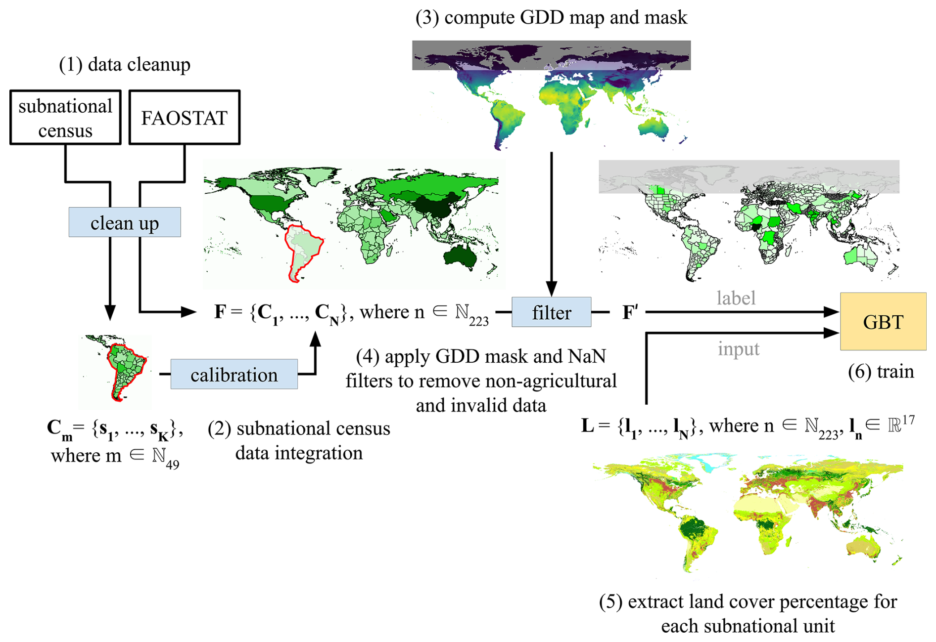
Figure 1 Data pre-processing and training pipeline. GDD: growing degree days; GBT: gradient boosting tree.

2.2 Deployment and post-processing pipeline

The second phase of analysis involves model deployment and post-processing (Fig. 2), which includes the following key steps:

1. Computation of land cover percentage for each 0.083 × 0.083 grid cell. The global land coverage map is segmented into grids which are then used as inputs for the trained model.

2. Cropland, pasture and other area prediction. The GBT model predicts a probability distribution for each land class over each deployment grid cell.

3. Regional masking. Apply masks to exclude non-agricultural regions (e.g. high aridity, low GDD).

4. Computation of weight matrices to match model inputs. Weight matrices are computed between masked outputs and model inputs with pycnophylactic interpolation.

   Calibration. The smoothed weight matrices are applied back to the model predictions, refining the outputs in each iteration to calibrate.

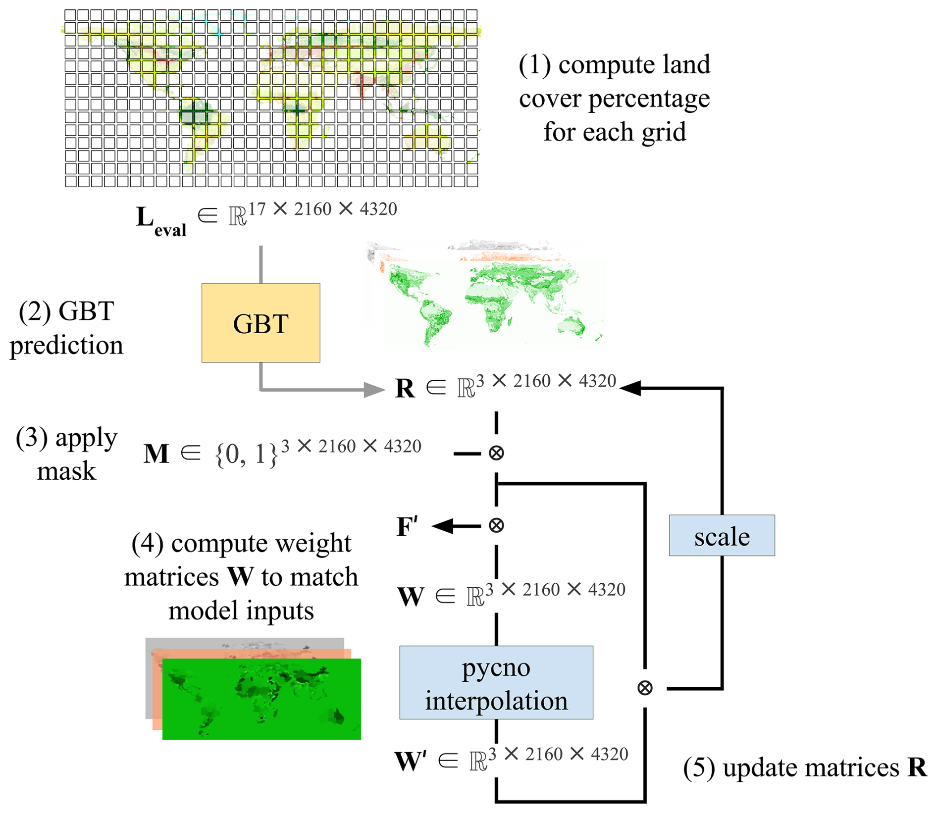
Figure 2 Data evaluation and post-processing; GBT: gradient boosting tree.

3 Input data

3.1 Agricultural inventory data

We compiled global cropland and pasture extent data from agricultural inventories and censuses over 2013–2017 (to represent circa 2015), following methods described in Ramankutty et al. (2008). Briefly, we first compiled national statistics for cropland area and pasture area from UN FAOSTAT (https://www.fao.org/faostat, last access: 1 April 2022) for the years 2013–2017, and took the mean of these to represent 2015. These data represented a national base layer of the absolute hectarage and proportions of cropland and pasture, which we then went on to replace with subnational statistics where available as explained below.

The baseline definitions, from the FAO, are as follows:

Cropland. This is land used for cultivation of crops, including areas under “Arable land” and “Permanent crops”, each of which is detailed below for completeness:

• Arable land. This describes the land used for cultivation of crops in rotation with fallow, meadows, and pastures within cycles of up to 5 years; it is the total of areas under “Temporary crops”, “Temporary meadows and pastures”, and “Temporary fallow”. Arable land does not include land that is potentially cultivable but is not cultivated.

• Temporary crops. This describes the land used for crops with a less-than-1-year growing cycle, which must be newly sown or planted for further production after the harvest. Some crops that remain in the field for more than one year may also be considered as temporary crops e.g. asparagus, strawberries, pineapples, bananas, and sugar cane. Multiple-cropped areas are counted only once.

• Temporary meadows and pastures. This describes land temporarily cultivated with herbaceous forage crops for mowing or pasture as part of crop rotation periods of less than 5 years.

• Temporary fallow. This describes land that is not seeded for one or more growing seasons. The maximum idle period is usually less than 5 years. This land may be in the form sown for the exclusive production of green manure. Land remaining fallow for too long may acquire characteristics requiring it to be reclassified, as for instance “Permanent meadows and pastures” if used for grazing or haying.

• Permanent crops. This describes land that is cultivated with long-term crops which do not have to be replanted for several years (such as cocoa and coffee), land under trees and shrubs producing flowers (such as roses and jasmine), and nurseries (except those for forest trees, which should be classified under “Forestry”). Permanent meadows and pastures are excluded from Permanent crops.

Pasture. This is land in Permanent meadows and pastures, land that is used permanently (5 years or more) to grow herbaceous forage crops through cultivation or naturally (wild prairie or grazing land). Permanent meadows and pastures on which trees and shrubs are grown should be recorded under this heading only if the growing of forage crops is the most important use of the area. Measures may be taken to keep or increase productivity of the land (i.e., use of fertilizers, mowing or systematic grazing by domestic animals). This class includes the following:

• grazing in wooded areas (agroforestry areas, for example);

• grazing in shrubby zones (heath, maquis, garigue);

• grassland in the plain or low mountain areas used for grazing, including land crossed during transhumance where the animals spend a part of the year (approximately 100 days) without returning to the holding in the evening (mountain and subalpine meadows and similar) and steppes and dry meadows used for pasture.

We then added subnational statistics for countries using a strategic search: (1) starting with major agricultural countries i.e. those included in the union of the 15 countries with highest global cropland or pasture area for 2015 (total 22 countries); (2) collecting subnational data for all EU countries from EUROSTAT (https://ec.europa.eu/eurostat, last access: 1 April 2022) (total 29 countries); and (3) finding the union of African countries with the highest cropland or pasture area, and selecting the top 10 countries of that union (which we found to be poorly represented in steps 1–2) (total 18 countries). Our resulting list consisted of 62 unique countries covering 81.6 % of global cropland and 82.1 % of global pasture area. With our priority search countries in hand, we searched each of these countries' national census bureau, ministry of agriculture, statistics office or other government entity websites for agricultural censuses or statistical yearbooks circa the year 2015 (our target was 2013–2017; in 12 cases where census data was not available in that range, we used data as early as 2007 or as late as 2018).

In each census or statistical yearbook, we searched for administrative level 1 information (i.e., one level below national) on the total area of cropland and pasture. This choice of administrative level was also strategic as it allowed for increased speed in data acquisition compared to prior work (e.g. Ramankutty2008) that used an exhaustive search at the highest resolution census input data possible. When necessary (i.e. outside the research team's language ability), we translated entire documents using Google Translate's document upload feature. We searched in these documents for statistics that aligned with the FAO definitions above. We note that reported definitions from state records are not always consistent with the FAO. In these cases we undertook case by case judgements on which statistics to include; all exact wordings from the source data used in the subnational statistics are included in Table C1 for full reproducibility. Note that pasture definitions for Saudi Arabia are massively different between the FAOSTAT and subnational statistics and it was therefore removed (although we make predictions for it, see later); see Ramankutty2008 for a discussion of this. We then extracted relevant tables and converted all units to hectares. Note that we could not find publicly available agricultural inventory data for some countries from our list during our search years, or found information on cropland area but not on pasture area; these countries were excluded from the model (Table C1). In total we found 49 countries that fit our criteria with subnational data, covering ∼ 73 % of the global cropland and ∼ 63 % of the global pasture.

3.2 Satellite data

We used data from the Moderate Resolution Imaging Spectroradiometer (MODIS) Land Cover Type (MCD12Q1) Version 6 at 500 m resolution (Sulla-Menashe and Friedl, 2018). We specifically selected the “Land Cover Type 1” layer, which labels land cover class in each pixel using the International Geosphere-Biosphere Programme (IGBP) classification scheme (see Table 3 in Sulla-Menashe and Friedl (2018) for the class definitions). We applied a temporal mode scheme to derive the most common land cover over 2013–2017 and determined that value as being the representative land cover for 2015 (the mode is designed to account for interannual fluctuations and noise in the data). A copy of the input land cover data used in the analysis is shown in Fig. 3c.

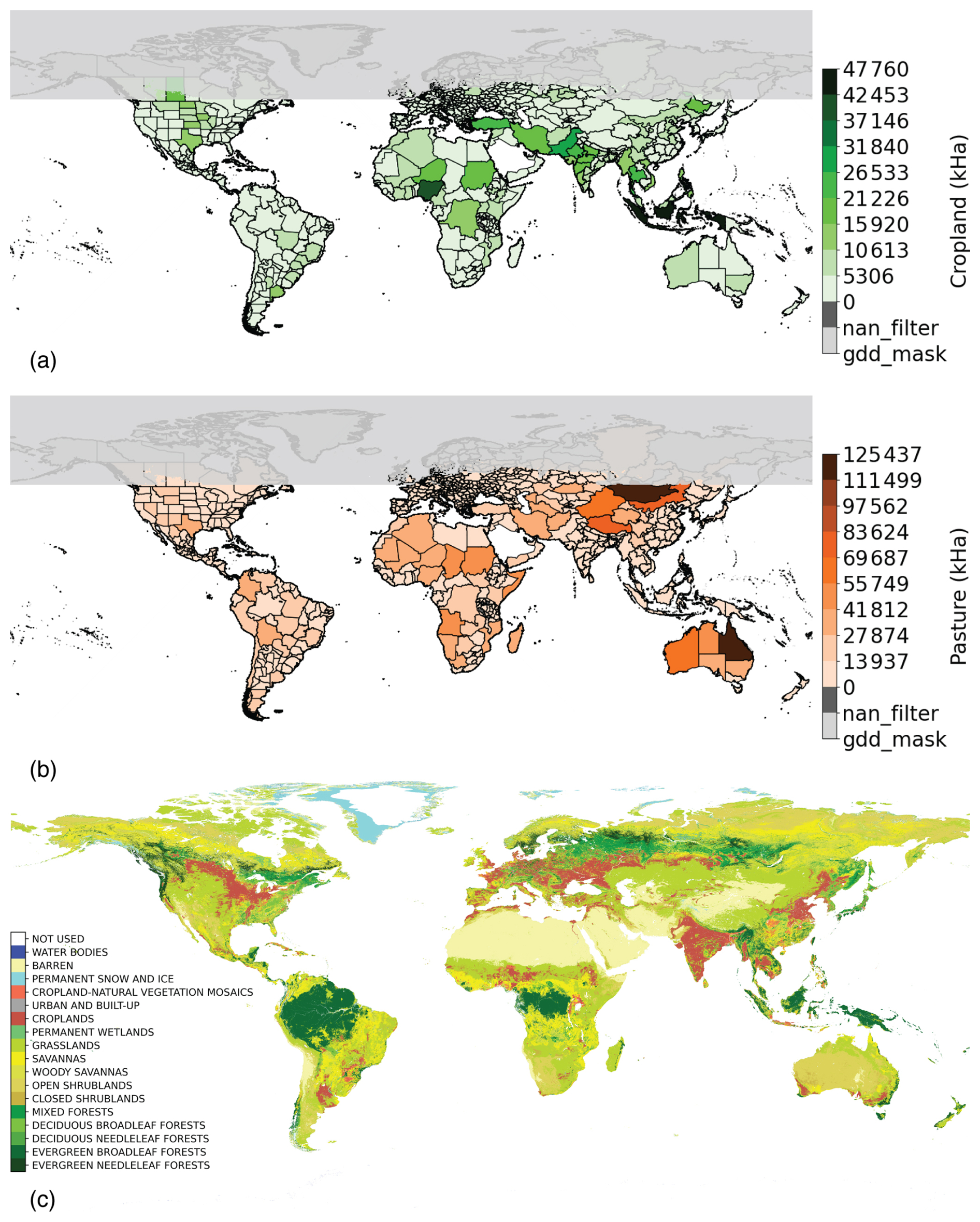
Figure 3 (a) Subnational and FAOSTAT merged input cropland after applying NaN and GDD filters, (b) subnational and FAOSTAT merged input pasture after applying NaN and GDD filters, and (c) the MCD12Q1 land cover map.

3.3 Pre-processing

FAOSTAT serves as the national base layer for our analysis, containing a total of 223 country level observations, which we denote as the set F={C_n where n ∈ N₂₂₃}. Each element of C in the set F represents a unique country level observation. Each country with subnational level data has multiple admin level 1 observations in a country: we denote this set as S={D_m} with K admin level 1 units, $D_m=\mathit{\{}{s}_{\mathrm{1}},\mathrm{\dots },s_K\mathit{\}}$ where m∈N₄₉ for 49 country records. Data source details are shown in Table C1.

The first step in the pre-processing pipeline is to decide whether or not to apply a calibration to match subnational statistics to the FAOSTAT reported national values or not. We offer options for choosing this in our codebase (any country may be calibrated to any label, subnational or national), although for this paper we consider national statistics as truth - as this is the version which our users most frequently use. The calibration process is as follows. It is given that D_m∈C_n where a country record occurs in both FAOSTAT and the subnational census set, and so a factor is formulated for any outcome of interest as $C_n/{\sum }_{i=\mathrm{1}}^K{s}_i$ if calibration is set true, otherwise 1. This factor is then multiplied to each sample in set D_m. After calibrating the censuses set, we merge it with the FAOSTAT set, with the dataset formulated as $F{}^{\prime }=\left\{C_n\mathrm{|}n\notin P\right\}\cup \mathit{\{}{D}_m\mathrm{|}m\in P$ where $P=F\cap S$.

Second we apply two spatial filters to pre-process the data prior to modelling: an NaN filter and growing degree day (GDD; base 5 °C) (SAGE, 2022) filter. The purpose of the first, the NaN filter, is to remove any data sample that has no data (or NaN) for the cropland or pasture percentage label. Our approach involves conducting evaluations for each subnational census sample. If the total geographical area of administrative level 1 units with missing cropland or pasture percentage label exceeds 30 % the total geographical area of the country, FAOSTAT level data was used instead for that country and the subnational data excluded from the model. We do this because our model relies on a complete probability distribution for each observation.

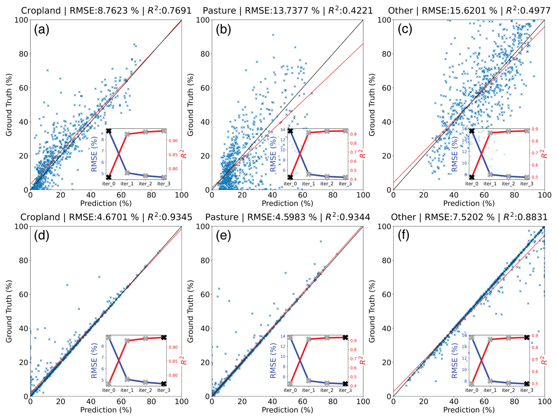
Figure 4 Observed vs Predicted plots (scatter plot) on re-aggregated scale after bias correction iterations. Cropland, Pasture and Other land use; (a, b, c) Iteration 0; (d, e, f) Iteration 3.

The purpose of the second, the GDD filter, is to retain any sample that lies within a GDD mask (see Fig. 3). We follow similar but more stringent criteria to Ramankutty2008, but where any non-cropland in MCD12Q1 (not the mosaic classes) above 50° N that has less than 1500 °C d⁻¹ GDD, the land is assumed to be too cold for agricultural production. Since observations (administrative units) can be partially covered by the GDD filter, we also introduce an acceptance ratio for the inclusion of an observation. For a given sample, either admin level 1 or country level, if the ratio between the area included after the GDD filtering step (i.e. it includes some portion of the area above 1500 °C d⁻¹) and the total area of that sample which is unmasked is less than our acceptance ratio (0.95), that sample is removed.

The processed and masked dataset for cropland and pasture, containing 715 administrative units (174 admin level 0, 541 admin level 1), is shown in Fig. 3a and b respectively. Admin level 1 units removed by each filter are marked with different colour codes.

To convert the dataset into a format for modelling, we add 17 attributes representing the percentages of 17 land cover types from MCD12Q1 product for each observation. The model output labels are percentages of cropland, pasture and other land (neither cropland nor pasture) in a given observation. We also include an observation weighting column for each row using the total geographic area of each observation. A higher weighting factor will give that corresponding observation more weight during model fitting.

Mismatches between subnational and national statistics are well known (Ramankutty et al., 2008; Ramankutty and Foley, 1998). For cases where sum of cropland and pasture exceeds 100 % due to calibration, these subnational observations were linearly scaled to a probability distribution prior to training. As we have explained above, we have factored our code in a way that makes it easy to update these parameters for more specific use cases.

4 Model

4.1 Setup

We modelled the relationship between the proportion of cropland, pasture, and other in an administrative unit to the proportion of each satellite-based land cover in those units. We used this model to downscale the proportion of each agricultural land use onto a gridded surface taking advantage of the higher spatial resolution of the satellite data. The basic model we employed was a gradient boosting tree (GBT) with a weighted multinomial logistic loss function defined in Eq. (1). The GBT implementation we use adopts a one-vs-rest classification approach, where three models fk(x) are trained for each class label (cropland, pasture, other).

$$\begin{array}{}\text{(1)}& L_i={\sum }_{k=\mathrm{1}}^K-{\mathit{\omega }}_i\left(y_{i,k}\log \left({\widehat{y}}_{i,k}\right)\right)\end{array}$$

In the loss function (1), we define $i=\mathrm{1},\mathrm{2},\mathrm{3},\mathrm{\dots },N$ for N total number of training samples and ω is the weight assigned to each sample based on the geographic area in that administrative unit. y_i,k is the census-derived probability for sample i in class k and ${\widehat{y}}_{i,k}$ is the predicted probability. The overall predicted probability for sample i can be expressed in terms of the softmax of model f_k(x) in Eq. (2).

$$\begin{array}{}\text{(2)}& {\widehat{y}}_{i,k}=\mathit{\sigma }\left(f_k\left(x_i\right)\right)={\displaystyle \frac{e^{f_k\left(x_i\right)}}{{\sum }_{l=\mathrm{1}}^K{e}^{f_l\left(x_i\right)}}}\end{array}$$

We use this model for a number of practical reasons: first is its ability to produce stable predictions despite multicollinearity in the predictor matrix (unlike a linear model estimated using least squares) and second is its ability to capture higher order interactions amongst the predictors without need for pre-specification. Our choice of loss function was driven by the biophysical constraint in that the proportions of different land classes within an administrative unit (e.g. cropland, pastureland and other) must all fall between 0–1. We fit the model using the h2o.ai framework (h2o.ai, 2022) which is fully parallel and readily supports the per-row observation weights which we use to incorporate area weighting in the model.

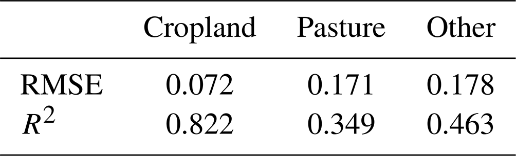
The five key hyperparameters (maximum tree depth = 5, column sampling rate = 0.5, number of trees = 75, learning rate = 0.1, and minimum number of observations per leaf split = 5) were selected using 10-fold spatial cross-validation on the 715 administrative units. More specifically, we use a 9:1 training and testing split, where the test set is uniformly random sampled across all available geospatial units. During spatial cross-validation within the training set, each fold of the validation set is sampled by blocks of regions that are close to one another in space. We use RMSE and R² as metrics to evaluate the initial model performance (i.e. against the test set). The results are shown in Table 1, illustrating high fits at the administrative unit level.

Table 1 RMSE and R² of trained GBT on test set.

4.2 Deployment

A histogram operator is then applied to each block matrix to obtain the percentage of occurrences of each land cover class in that block. Our trained model then predicts, over all batches of block matrices, the proportion of cropland, pasture land and other land on a 5 arcmin (∼ 10 km × 10 km at the Equator) lattice.

4.3 Post-processing

For post-processing, we introduce a bias-correction step to bridge the unknown relationship between the block matrix unit during deployment and administrative unit level during training. Each pixel of our output map falls within a boundary R_n of a training label; y_n is denoted as ${\widehat{y}}_{n_{ij}}$ for $\left(i,j\right)\in R_n$. Each ${\widehat{y}}_n$ contains 3 channels, representing cropland, pasture, and other land use percentages. The bias-correction factor (tuple) for each pixel in R_n is therefore $b_n=y_n{\sum }_{(i,j)\in R_n}{A}_{ij}/{\sum }_{(i,j)\in R_n}[{\widehat{y}}_n\otimes A{]}_{i,j}$, where $A\in R^{\mathrm{2160}\times \mathrm{4320}}$ is the global area matrix, and ⊗ is the element-wise multiplication symbol. This factor (tuple) is then multiplied to all pixels in R_n as ${\widehat{y}}_{n_{ij}}^{\prime }=b_n{\widehat{y}}_{n_{ij}}$. In simple terms, we use this post-processing step to ensure convergence between the pixel-level deployment and the administrative unit-level reported values for geographies where that data exist.

To maintain the probability distribution we further apply a scaling operator to each pixel to force the sum of factored proportions back to 1. The operator is formulated as ${\widehat{y}}_{n_{ij}}^{\prime }\leftarrow {\widehat{y}}_{n_{ij}}{}^{\prime }/\sum {\widehat{y}}_{n_{ij}}{}^{\prime }$.

To remove boundary artefacts between administrative units, we then apply pycnophylactic interpolation (Tobler, 1979) with relaxation at the end of each bias-correction iteration on all weights b_n. The property of pycnophylactic interpolation ensures the regional sum remains unchanged after smoothing, which does not interfere with the effectiveness of bias-correction steps. Specifically, the mean filter in this process we used is [0.5, 0, 0.5] with a converge value of 3 and relaxation 0.2.

The spatial patterns of predicted outcomes within a subnational unit result from the cross-validated model. We do however force convergence of these subnational predictions to match the input data. Also, we note our model is global, unlike previous regionally parameterized models from the circa 2000 agricultural land product. We do this due to our focus on rapidly acquiring label data at administrative level 1, rather than previous attempts, which included data down to administrative level 3. Due to the global nature of this model, a number of additional corrections are made. In each iteration of bias-correction, we apply the GDD mask, water body mask, and an aridity mask (Zomer et al., 2022) to the output map to remove non-agricultural regions that otherwise would get re-introduced by bias correction back to administrative level data. Our aridity mask uses a threshold of high aridity (0.05 aridity index), used in a similar vein to the GDD mask, to remove lands unsuitable for rainfed agriculture and is updated with irrigation equipped areas at a 1 % threshold (Mehta et al., 2022). This process ensures that these areas are maintained in the final product in highly arid regions throughout bias correction as they are particularly important for irrigated cropland in dry areas.

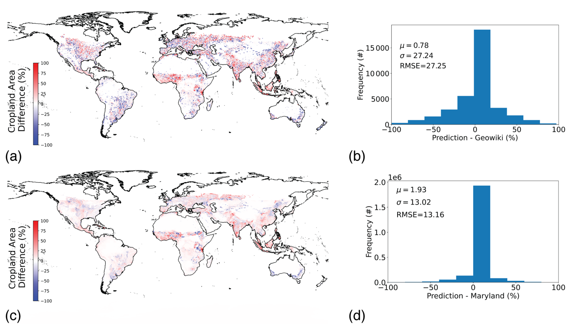
Figure 5 Cropland external validation and intercomparisons (a) Scatter points of intercomparison against Geo-Wiki cropland data; (b) Histogram of errors for Geo-Wiki comparison; (c) Map difference of intercomparison against University of Maryland cropland map; (d) Histogram of errors for University of Maryland comparison.

A specific mask for Australia was employed, as was previously done with Ramankutty2008, due to consistently poor performance of the globally parameterized model in that region. For this country mask we rely on locally available land use data developed by the Australian Department of Agriculture Water and the Environment: the Land Use based on Agricultural Commodities at 250 m 2015–2016 (ABARES, 2022). We apply two simple rules: for pasture area predictions we mask everything identified by ABARES as “Non agricultural land” and for cropland we mask everything defined as “Non-agricultural land” OR “Grazing”. Here Grazing (see Fig. B2) includes modified and natural grazing and was introduced to primarily to exclude the large extensive grazing systems in the region. Nearest neighbour resampling of the original 250 m labels to 0.083° prior to masking maintained broad scale ABARES cropland patterns (see Fig. 6a).

5 Assessment

5.1 Assessment at the spatial scale of administrative units

Validation of the full modelling and post-processing pipeline with the input training data was completed by aggregating our final post-processed predictions at the gridded lattice to the level of the administrative unit used in training and comparing proportional coverage estimates to survey reported cropland and pasture proportional coverage in that unit. We undertook this validation prior to, during, and at the end of our postprocessing steps outlined in 4.3. Scatter plots of these comparisons are shown in Fig. 4 along with summary statistics using RMSE and R². In general, we found our model to perform well for estimating cropland and pasture in its raw form of the deploy (i.e. with no bias-correction, iterations = 0, Fig. A1) and to converge with input data for all three classes after three bias-correction steps (iterations = 3).

5.2 Assessment at the spatial scale of predictions

We employed an independent dataset for validation of the predicted proportional land cover at the 5^′ level for cropland. These data were collected through the crowd-sourced Geo-Wiki platform, in which participants identified the proportion of cropland in nearly 36 000 sampling units of 300 m × 300 m distributed around the globe (Laso Bayas et al., 2017; See, 2017). Here we took the average percentage coverage of all Geo-Wiki observations at a given point within each 0.083 × 0.083° grid cell. This validation dataset was chosen for its independence, broad geographic distribution, and transparency and, critically, because it is not a modelled product itself (unlike, say, cropland classification products, although see below for intercomparisons with other modelled products). One thing we do note, however, is that there are no global cropland products for validation or intercomparisons at the spatial scale of the predictions that incorporate the full spectrum of croplands as we define here; Geo-Wiki excludes perennial crops, agroforestry plantations, palm oil, coffee, and tree crops for example, and the University of Maryland product is similarly restricted to annual crops (Potapov et al., 2021).

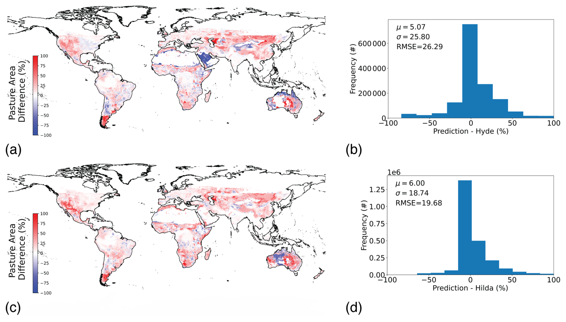
Figure 6 Pasture map intercomparisons against (a) HYDE and (c) HILDA+. Histogram of errors for (b) HYDE and (d) HILDA+ comparison.

Notably, newer datasets have been developed to fill this gap (i.e. which map tree crop area rather than the annual crop estimates used in other cropland definitions), such as the World Resource Institutes Spatial Database on Planted Trees (SDPT) (Richter et al., 2024). On visual inspection of these additional data (not shown) we do find a spatial correspondence that indicates differences between our cropland product (which incorporates all crop types, including trees) and other global cropland maps (such as the Maryland or Geo-Wiki cropland maps, which are only focussed on annual crops) can be explained by areas mapped in SDPT, particularly Indonesia, some regions of West Africa, and southern Spain.

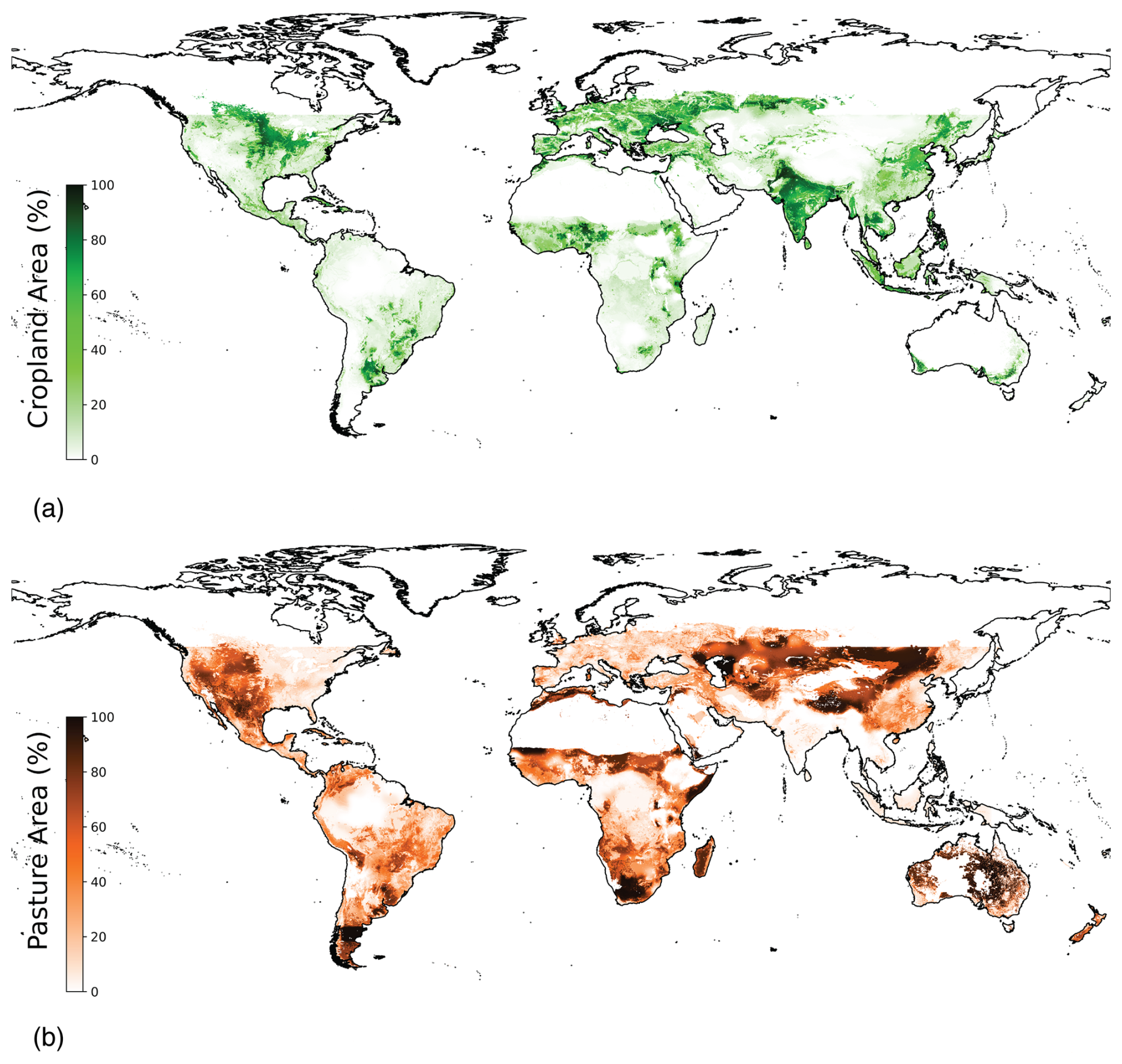
Figure 7 (a) Cropland and (b) Pasture final product at iteration 3. See Fig. A1 for iteration 0.

Table 2 Summary of final product total areal estimates.

A comparison of our predicted cropland proportional coverage and those from samples of the independent Geo-Wiki campaign is shown in Fig. 5. In this comparison, we take the difference between the common points and show the level of agreement with our final product and this independent dataset in terms of mean difference (0.78 percentage points) and standard deviation of the difference (27.24 percentage points). Despite the extremely close alignment on average globally, some notable differences exist geospatially, e.g. we show pixels with higher percentage cropland in the Canadian Prairies, West Africa, West India, and Russia, but lower cropland in South America, South East Africa, and Southern Australia. Notably no globally consistent independent pasture data exist for external validation at the scale of predictors, although we did conduct product comparisons for both cropland and pasture to check how our predictions aligned with other independent datasets as explained below.

5.3 Intercomparisons at the spatial scale of gridded predictions

We conducted product intercomparisons for both our final cropland and pasture products. For cropland we compared our data to the University of Maryland global cropland dataset (at 30 m resolution) (Potapov et al., 2021). As these data are sequences of time ranges, we take the average coverage for 2012–2015 and 2015–2019 to arrive at a 2015 estimate of 30 m categorical cover, which we aggregated to 5^′ to estimate proportional coverage in each grid cell. A comparison of our 2015 estimates with the Maryland data are shown in Fig. 5, showing the agreement with the mean (1.93 percentage points) and standard deviation of differences (13.02 percentage points). This agreement is even tighter than with the Geo-Wiki dataset.

For pasture, we compared our predictions to two global scale pasture maps, HYDE (Klein Goldewijk et al., 2017) and HILDA+ (Winkler et al., 2021) (Fig. 6). These products are mainly focused on land use/land cover change but also contain static maps for the year 2015. They are both based on a satellite-based land cover map whereby classes are assigned to be pasture, either heuristically (for HYDE) or by spatial overlap with the Gridded Livestock of the World livestock abundance data (for HILDA+). Both are calibrated to FAOSTAT pasture statistics. We found agreement on average between our product and these maps, albeit with spatial variability, with a mean difference of 5.07 (SD 25.80) percentage points with the HYDE product and 6.00 (SD 18.74) percentage points with the HILDA+ product. Our GDD masks in comparison to HYDE and HILDA+ do impact on differences. In total, our GDD masks remove 1 106 005 km² of areas considered in Hyde (∼ 2 % of total GDD mask area, 3.5 % of pasture area) and 163 865 km² in of areas considered in HILDA+ (∼ 0.3 % of total GDD mask area, 0.05 % of pasture area).

A well-known issue with pasture maps is the difficulty of defining what is a “pasture”; this could explain some of the spatial discrepancies. For example, Fig. 6a in our global comparison with HYDE shows a large difference in Saudi Arabia, with HYDE being calibrated to FAOSTAT values but our model relaxing that constraint for this country. As a complement to these global comparisons, we also examined a number of region or country specific pasture datasets in more detail. We did this for Australia, Brazil, and the conterminous USA. These intercomparisons (Fig. B1a–h), show the best alignment in Europe, followed by Brazil, the USA, then Australia. These additional intercomparisons with national level datasets demonstrate broad alignment, but also some spatial disagreement between pixel level predictions on average with those made by independent groups, models, and methods.

6 Data availability

The cropland and pasture data are available for download in GeoTIFF format at the permanent link at Zenodo (Mehrabi et al., 2024; https://doi.org/10.5281/zenodo.11540554), along with meta-data and instructions for use. Here you will find the FAOSTAT calibrated product (as presented in the main text) for end users, but a subnational trained product could also be generated with the provided pipeline.

7 Code availability

In addition to providing this data update, alongside this publication we also for the first time release software to enable the reproduction of this dataset as well as future updates in a relatively easy fashion. All of the underlying training data, scripts, and the trained model are stored on the Zenodo public repository link (Mehrabi et al., 2024, https://doi.org/10.5281/zenodo.11540553). Forks may be made from the GitHub repository (https://github.com/Better-Planet-Laboratory/global-agland-2015, last access: 1 April 2025).

We provide this material as a service to the community so that future updates, for example to the year 2020 and beyond, may be done as a community effort. Importantly, because of the streamlined pipeline, this work is easily done with modest computational resources. It takes on average 24.71 s for training and 2.07 h for deployment for each iteration and outcome on an Apple M1 Max processor with 32 GB memory (deployment time varies significantly when changing convergence settings in pycnophylactic interpolation). This code base resource also allows researchers to “slot” in different land cover datasets, which may be of interest for producing finer scale predictions, e.g. with the ESA's 10 m land cover dataset. While requiring higher computational capacity, this may be useful for other applications, if relevant independent test data or intercomparisons provide sufficient confidence in predictions at that scale.

8 Final product

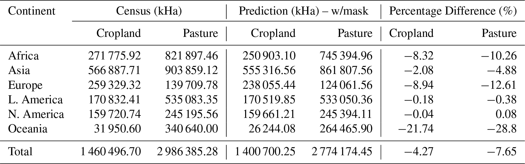
Our final product of the distribution of agricultural lands for the year 2015 at 5^′ resolution is shown in Fig. 7a–b. For general benchmarking, we computed regional and global summaries of total cropland and pasture. Our total estimate of cropland area in the year 2015 is 1 400 700 Kha whereas pasturelands encompass 2 774 174 Kha (compared to FAOSTAT values of 1 460 496 and 2 986 385 Kha respectively. When compared to the totals of the input data used in the model, these estimates are around 4 % lower than the census dataset estimates for cropland and 7.5 % lower for pasture, although geographic variation does exist for some countries and regions that deviate from these means. For example, on aggregate our product shows 8.3 % lower cropland and 10.3 % lower pasture in Africa than the census data totals (see Table 2 for full regional comparisons).

We note at least two sources of error a priori that likely drive these aggregate differences: (1) some residual error remains as shown in Fig. 4 after iteration 3 of the bias correction (which is assumed to also carry to locations where we do not have training data); and (2) we apply a fairly strict GDD mask for growing locations, which eliminates some administrative units where there may be agricultural lands (see Ramankutty2008 for a discussion on this), although we relax this restriction over known satellite-classified cropland in Europe and Canada to mitigate this underestimation.

One important thing to note about these data is their intentional use. As for Ramankutty2008, these data are intended for use in global modelling studies. This statement is even more important perhaps than the ∼ 2000 product because of the global scale of the model and coarser input labels. There are errors that result from training a model using administrative level 0/1 data and deploying at a grid cell as outlined here. There are further constraints due to parameterizing a single model that is applied across the entire planet. As such we recommend regional focussed analyses to seek more fine-tuned national or regional data. Furthermore, we stress these data should not be used for time series analysis with the 2000 product due to errors in the underlying MODIS data and the different modelling pipelines. At the same time, all said, we have taken reasonable care to make corrections. This update is for users that require global data that covers comprehensive cropland and pasture definitions and is numerically consistent between land use estimates.

Appendix A

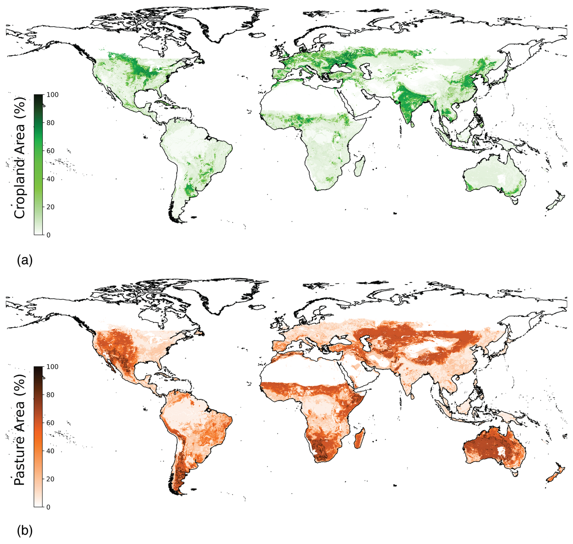
Figure A1 (a) Cropland and (b) Pasture final product at iteration 0.

Appendix B

B1 Pasture intercomparison methods

We compared our pasture product to a number of independent region and country products as shown below (Fig. B1). The map for Australia is the Land Use of Australia 2015–2016 at 250 m resolution (Fig. B2) and was modelled based on Advanced Very High Resolution Radiometer (AVHRR) satellite imagery and 2015–2016 census data using a Markov Chain Monte Carlo algorithm (ABARES, 2022). The map for Brazil is a 2015 land use map produced by MapBiomas at 30 m resolution using Landsat 8 satellite imagery and random forest classification (Parente et al., 2017) and was found to have an overall accuracy of 87 %. The map for Europe is a 30 m map of pastures for 2015 based on LUCAS (Land Use and Coverage Area frame Survey) and CLC (CORINE Land Cover) maps via spatiotemporal ensemble machine learning (Witjes et al., 2022). The reference map for the USA is a combination of the National Land Cover Database map for 2011 (USGS, 2011) which is based on Landsat imagery, multi-source training data, and a decision tree-based classification algorithm and the USDA rangelands map (Reeves and Mitchell, 2011). Both inputs use 30 m resolution. We combined these two maps for the USA because our subnational data combines data from the census (grassland pasture and range in farms) with data from the Bureau of Land Management (grassland pasture and range not in farms).

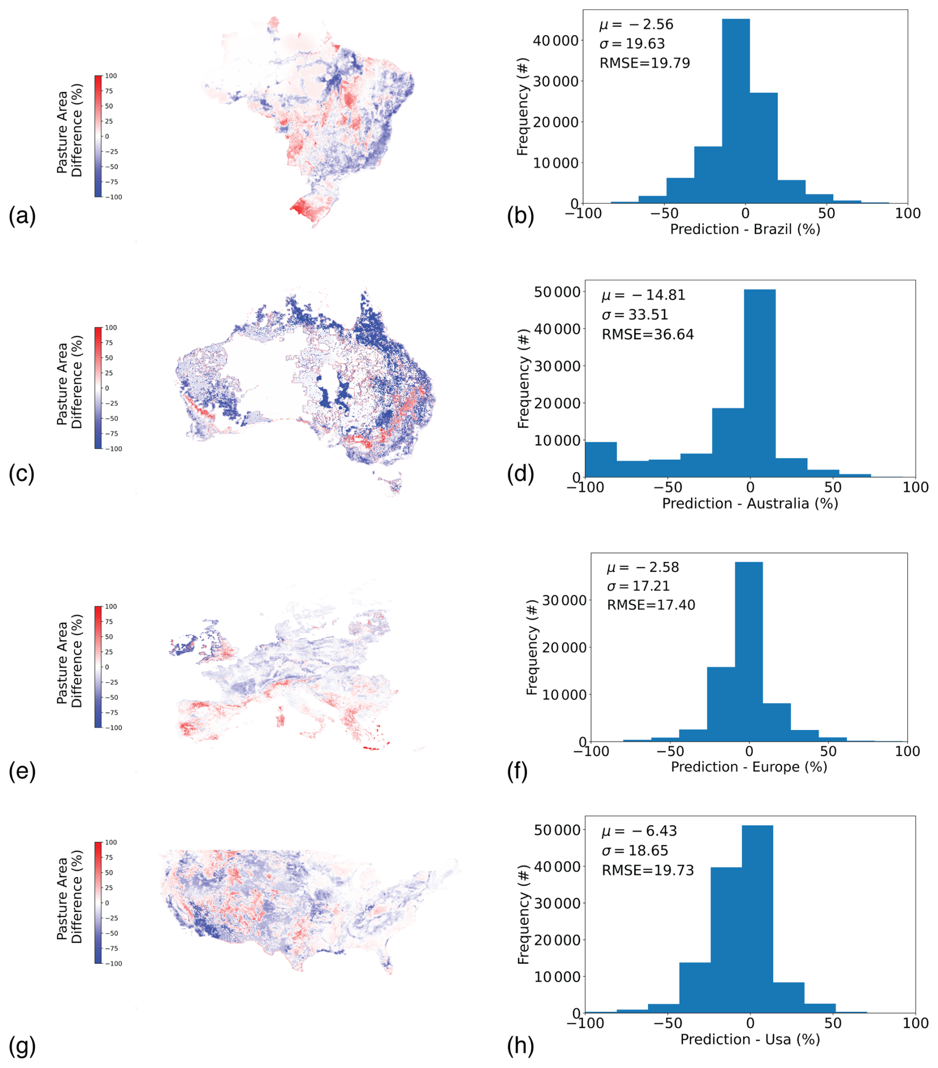
Figure B1 Pasture map intercomparisons against (a) Brazil, (c) Australia, (d) Europe, and (g) USA; Histogram of errors for (b) Brazil, (d) Australia, (f) Europe, and (h) USA.

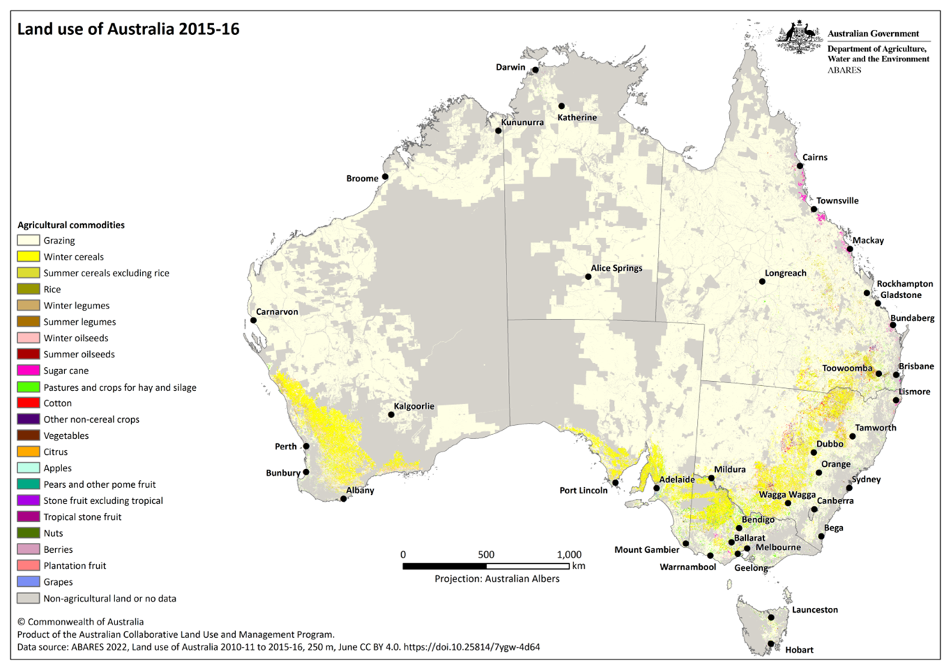
Figure B2 ABARES land use map used in this study for Australia mask creation.

Appendix C

Table C1 All countries for which we searched for subnational data. See main content for selection criteria for this list.

NA: not available.