cigChannel: a large-scale 3D seismic dataset with labeled paleochannels for advancing deep learning in seismic interpretation

Identifying paleochannels in 3D seismic volumes (seismic paleochannel interpretation) is essential for georesource development and offering insights into paleoclimate conditions. However, it remains a labor-intensive and time-consuming task. Deep learning has shown great promise in automating seismic paleochannel interpretation with high efficiency and accuracy, as demonstrated in similar image segmentation tasks in computer vision (CV). Yet, unlike the CV domain, seismic exploration lacks a comprehensive labeled dataset for paleochannels, significantly hindering the development, application, and evaluation of deep learning methods in this field. Manual labeling of paleochannels in 3D seismic volumes is tedious and subjective, potentially leading to mislabeling that degrades deep learning model's performance. To address this, we propose a workflow to generate a synthetic seismic dataset, cigChannel, consisting of 1600 seismic volumes with over 10 000 labeled paleochannels. Each volume has a size of $\mathrm{256}\times \mathrm{256}\times \mathrm{256}$ samples. This is the largest dataset to date for seismic paleochannel interpretation, featuring geologically reasonable seismic volumes with accurately labeled meandering channels, tributary channel networks, and submarine canyons. A convolutional neural network (simplified from U-Net) trained on this dataset achieves F₁ scores of 0.52, 0.73, and 0.63 in identifying meandering channels, tributary channel networks, and submarine canyons in three field seismic volumes, respectively. However, the synthetic seismic volumes in the cigChannel dataset still lack the variability and realism of field seismic data, potentially affecting the deep learning model's generalizability. To facilitate further research, we publicly release the dataset (Wang et al., 2024, https://doi.org/10.5281/zenodo.10791151), data generation codes, and trained U-Net model (Wang, 2024, https://github.com/wanggy-1/cigChannel, last access: 5 July 2025), aiming to advance deep learning approaches for seismic paleochannel interpretation.

1 Introduction

Paleochannels are buried river channels that have been preserved in the geological record. They can not only provide insights into paleoclimate conditions (e.g., Leigh and Feeney, 1995; Nordfjord et al., 2005; Sylvia and Galloway, 2006) but also serve as reservoirs for groundwater (e.g., Revil et al., 2005; Samadder et al., 2011), geothermal energy (e.g., Crooijmans et al., 2016; Kang et al., 2022), ore deposits (e.g., Heim et al., 2006; Oraby et al., 2019), and hydrocarbons (e.g., Clark and Pickering, 1996; Bridge et al., 2000). Paleochannels can be identified in seismic volumes by their distinct shapes and sedimentary structures, which differ from the surrounding rock formations. Although paleochannels are considered as geobodies, interpreters are limited to viewing them slice-by-slice in seismic volumes. This limitation significantly increases the complexity and time of interpreting paleochannel bodies in large seismic volumes. Moreover, the historical tectonic movement may introduce deformations, such as foldings to the paleochannels, making them even more difficult to recognize.

To address those issues, automatic paleochannel identification methods based on 3D convolutional neural networks (CNNs) (Pham et al., 2019; Gao et al., 2021) have been developed. The 3D CNNs are designed to capture volumetric features by performing 3D convolutions (Ji et al., 2012). They have the advantage of handling paleochannels according to their 3D nature, as opposed to the slice-by-slice visual investigation of a human interpreter. This advantage is particularly significant when the paleochannels have been deformed by historical tectonic movements (e.g., folding and faulting), which disrupt their continuity and make them more challenging to track in a slice-wise view. Another notable advantage is their efficiency. Once trained, the network can rapidly identify paleochannels in a large seismic volume. However, the main limitation of applying CNNs for paleochannel identification is the lack of labeled paleochannel samples for training. Unlike deep learning for computer vision, which benefits from numerous large datasets with labeled images, such as ImageNet (Deng et al., 2009), COCO (Lin et al., 2014), and ADE20K (Zhou et al., 2017), there is no publicly available dataset of field seismic volumes with labeled paleochannels. To create such a dataset, one needs to access a large amount of field seismic volumes and correctly label the paleochannels. However, labeling paleochannels can be challenging, due to the complexity of field seismic volumes, and human bias may introduce uncertainty to the labels (Bond et al., 2007). The label noise produced by mislabeling will deteriorate the performance of supervised learning (Pechenizkiy et al., 2006; Nettleton et al., 2010). Additionally, the labeling process will be time-consuming and labor-intensive.

While creating a dataset by labeling paleochannels in field seismic volumes is expensive, an alternative solution is to use synthetic seismic volumes, which are generated through a series of simulation processes in order to mimic field seismic volumes. Although lacking in sophisticated features, the synthetic seismic volumes are controllable, allowing us to tailor the features that our network will learn to segment. Moreover, mislabeling can be avoided in synthetic seismic volumes since the locations of objectives are known during the simulation process. Synthetic seismic volumes have been proven effective as training data for CNNs to identify various objectives in field seismic volumes, such as faults (Wu et al., 2019; Zheng et al., 2019), seismic horizons (Bi et al., 2021; Vizeu et al., 2022), paleokarsts (Wu et al., 2020b; Zhang et al., 2024), and paleochannels (Pham et al., 2019; Gao et al., 2021). As for paleochannel identification, the synthetic seismic datasets created by Pham et al. (2019) and Gao et al. (2021) only simulate meandering channels, while the frequently observed tributary channel networks (e.g., Nordfjord et al., 2005; García et al., 2006; Darmadi et al., 2007) and submarine canyons (e.g., Deptuck et al., 2007; Gee et al., 2007; Covault et al., 2021) are not included. Considering the diversity of paleochannels in field seismic volumes, creating a dataset with various types of paleochannels is necessary for enhancing a CNN's generalizability.

In this paper, we propose a workflow (Fig. 1) for generating synthetic seismic volumes with three types of paleochannel and their labels. We first build numerous 3D models of meandering channels, tributary channel networks, and submarine canyons. Parameters that control the modeling process are randomized within reasonable ranges in order to increase the diversity of channel models. Second, we build seismic impedance models with multiple layers and place the channels at layer boundaries as impedance anomalies. Third, the impedance models are used to calculate seismic reflection coefficients, which are subsequently convolved with Ricker wavelets to create synthetic seismic volumes. Finally, channels in the seismic volume can be automatically labeled since their positions are already known. Using this workflow, we have created a dataset named cigChannel (Wang et al., 2024, https://doi.org/10.5281/zenodo.10791151) for deep learning-based seismic paleochannel interpretation. This dataset contains 1600 seismic volumes and labels of more than 10 000 paleochannels. Each seismic volume has a size of $\mathrm{256}\times \mathrm{256}\times \mathrm{256}$ samples. The effectiveness of this dataset has been validated by training a CNN to identify meandering channels, tributary channel networks, and submarine canyons in three field seismic volumes, respectively. It should be noted that, although we have significantly improved the diversity of paleochannels compared with previous datasets, there is no guarantee that this dataset covers every form of paleochannel in field seismic volumes. Therefore, a Python package of the dataset generation workflow (Wang, 2024) (https://github.com/wanggy-1/cigChannel, last access: 5 July 2025) is also provided for customizing paleochannels and facilitating further development (see Appendix C for demonstration codes).

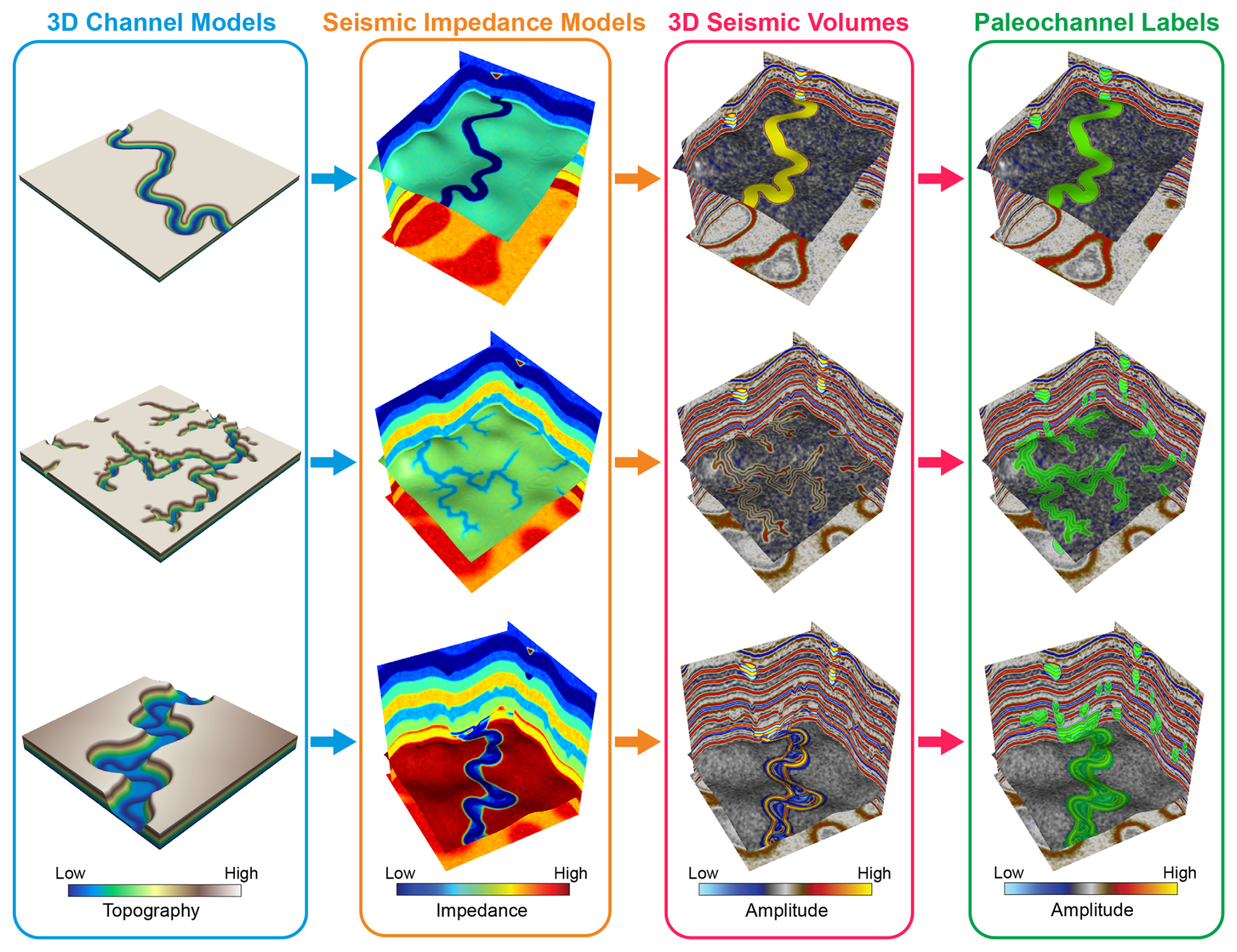
Figure 1 Workflow for generating the cigChannel dataset. First, we create 3D models of three types of paleochannel: meandering channels, tributary channel networks, and submarine canyons. Second, we build 3D seismic impedance models with multiple layers and place these channels at layer boundaries as impedance anomalies. Third, the impedance models are used to calculate seismic reflection coefficients, which are subsequently convolved with Ricker wavelets to create synthetic seismic volumes. Finally, seismic reflections of paleochannels are automatically labeled. Note that the channel models, seismic impedance models, and seismic volumes are all in the depth domain.

2 Dataset generation workflow

In this section, we will outline the dataset generation workflow, covering the steps for constructing 3D channel models and synthesizing seismic volumes. We will begin by describing the modeling process for meandering channels, tributary channel networks, and submarine canyons. Following that, we will explain how to build seismic impedance models based on these channel models and use the impedance models to generate synthetic seismic volumes.

2.1 Meandering channel modeling

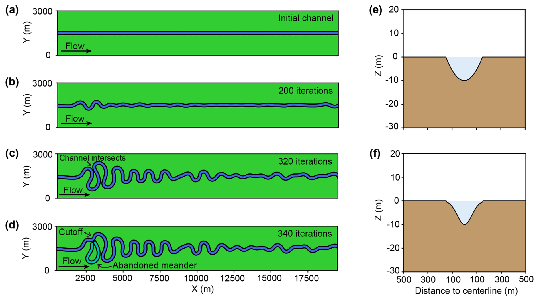
Figure 2 Meandering channel modeling process based on the open-source Python package meanderpy (Sylvester, 2021). (a) First, we create a straight channel with some minor perturbations. (b) Then the channel begins to migrate, leading to the formation of multiple meanders. (c) The channel curvature increases as the migration continues, eventually causing a channel intersection, where (d) the channel cutoff will occur, resulting in an abandoned meander. Lastly, (e) U- and (f) V-shaped channel cross-sections are used to define the channel topography.

Meandering channels are a common type of river channel that can be found in many seismic volumes (e.g., Noah et al., 1992; Carter, 2003; Wood, 2007; Wang et al., 2012; Alqahtani et al., 2017). They are distinguished by their sinuous paths. The continuous interaction between water and the riverbed can lead to erosion on the outer bank and deposition on the inner bank, causing the channel to migrate over time, increasing its curvature. The key to create a realistic meandering channel is to simulate its migration. For this purpose, we use the open-source package meanderpy (Sylvester, 2021), which employs a kinematic simulation method that computes the river migration rate as a weighted sum of upstream curvatures (Howard and Knutson, 1984; Sylvester et al., 2019). This simple kinematic model focuses on the influence of upstream curvatures on river migration and cannot capture complex processes such as compound meander formation without cutoffs (Frascati and Lanzoni, 2009). However, it is sufficient for generating morphologically realistic meandering channels. The meandering channel simulation process is demonstrated in Fig. 2. We start with a straight channel with some minor perturbations, which provide initial curvatures for channel migration (Fig. 2a). The channel migrates over time and forms meanders at its upstream (Fig. 2b). As the migration continues, curvature of the meander increases and eventually leads to channel intersection (Fig. 2c), where the channel cutoff will occur, resulting in an abandoned meander (Fig. 2d). The channel migration ends when the maximum number of iterations is reached. We neglect the abandoned channel and extract the centerline from a random segment of the most recent meandering channel, which has to be long enough to span a square grid of 256×256 cells with a cell size of 25 m after arbitrary rotation.

The centerline is then randomly placed on the grid and rotated by a random angle between 0 and 360°. Since meandering channels in field seismic volumes typically exhibit U- or V-shaped cross-sections (e.g., Zhuo et al., 2015; Alqahtani et al., 2017; Zeng et al., 2020; Manshor and Amir Hassan, 2023), we use simplified U- or V-shaped profiles to define the channel topography, as shown in Fig. 2e and f. The simplified U-shaped channel is defined as a parabolic function:

$$\begin{array}{}\text{(1)}& Z\left(x\right)=\left\{\begin{array}{ll}\mathrm{4}{D}_{\mathrm{c}}(x/W_{\mathrm{c}}{)}^{\mathrm{2}}-D_{\mathrm{c}},& x\le W_{\mathrm{c}}\\ \mathrm{0},& x>W_{\mathrm{c}}\end{array}\right.,\end{array}$$

where x is the Euclidean distance from the centerline to any point on the grid, D_c is the maximum depth of the channel (which will be denoted as channel depth hereafter for simplicity), and W_c is the channel width. The simplified V-shaped channel is defined as a combination of Gaussian and parabolic functions:

$$\begin{array}{}\text{(2)}& Z\left(x\right)=\left\{\begin{array}{ll}min\left[p\left(x\right),g\left(x\right)\right],& x\le W_{\mathrm{c}}\\ \mathrm{0},& x>W_{\mathrm{c}}\end{array}\right.,\end{array}$$

where p(x) is the parabolic function in Eq. (1) and

$$\begin{array}{}\text{(3)}& g\left(x\right)=-D_{\mathrm{c}}{\mathrm{e}}^{-\frac{x^{\mathrm{2}}}{\mathrm{2}(W_{\mathrm{c}}/\mathrm{4}{)}^{\mathrm{2}}}}.\end{array}$$

Although these simplified channel cross-sections may not precisely represent the real ones, they can capture their main features at a low computational cost. We create diverse topographic models of the meandering channel by randomizing the modeling parameters within reasonable ranges (see Table A1). Some examples are demonstrated in Fig. 5a, showing various meandering channels with different widths, depths, and meander wavelengths.

It should be noted that, in this study, we focus on identifying the most recent meandering channels in their migration histories. Therefore, all the meandering channel models only include the last channel form of the migration process. The corresponding sedimentary facies formed during the channel migration process, such as point bars, natural levees, and abandoned channels (or oxbow lakes), are not included. It is also worth noting that the width and maximum depth of each channel are fixed, while in nature they generally exhibit a certain degree of variability.

2.2 Tributary channel network modeling

A tributary channel network is a result of smaller rivers (tributaries) flowing into a large main river. It generally exhibits a branching or tree-like structure. To efficiently generate extensive tributary channel networks that are morphologically reasonable, we adopt the open-source package soillib (McDonald, 2020b), which offers a fast implementation of particle-based hydraulic erosion that can create a morphologically reasonable tributary river network in about 10 to 20 s (McDonald, 2020a).

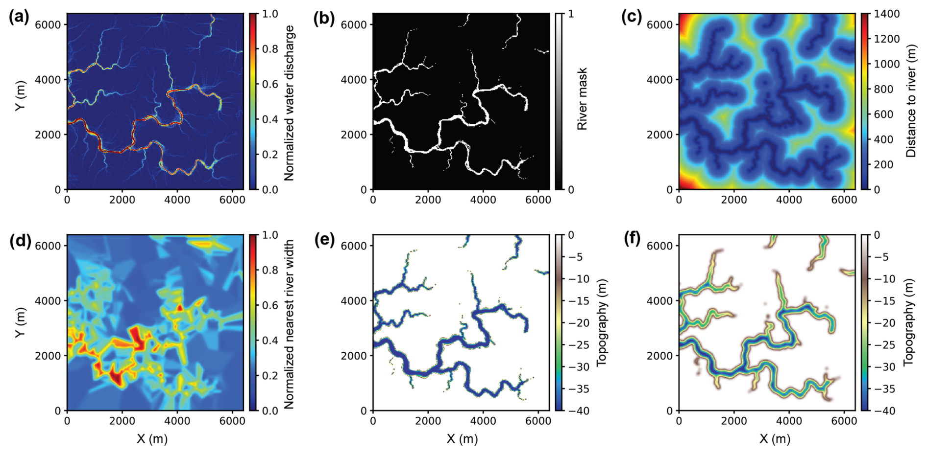
Figure 3 Tributary channel network modeling process based on the open-source package soillib (McDonald, 2020b). (a) First, we generate a map of normalized water discharge value using the soillib package. (b) Second, we create the river mask by binarizing the normalized water discharge with a threshold of 0.4, where discharge values greater than this threshold are considered as rivers. (c–e) Third, we compute (c) the Euclidean distance to rivers and (d) the normalized nearest river width, which are subsequently used to define (e) the channel topography. (f) Finally, to avoid abrupt topographic changes, a Gaussian filter is applied to create a smoothed channel topography.

The soillib package is programmed to spawn hundreds of thousands of water particles at random positions on a mountainous terrain generated by random Perlin noise. The water particles move across the terrain following classical mechanics and engage in mass transfer with the surface, eventually forming a tributary river network. Figure 3a shows a map of the normalized water discharge generated by soillib on a square grid of 256×256 cells with a cell size of 25 m. To define the river channel topography, we first binarize the normalized water discharge by a threshold of 0.4, where discharge values greater than this threshold are considered as rivers (Fig. 3b). Next, we compute the Euclidean distance from the river to each point on the grid (Fig. 3c) and the normalized width of the nearest river (Fig. 3d). The normalized width of the nearest river is determined by the value of normalized water discharge. Rivers with higher discharge will have larger width. We then define the channel topography using a parabolic function similar to that in Eq. (1):

$$\begin{array}{}\text{(4)}& Z_i\left(x_i\right)=min\left[\mathrm{4}{D}_{\mathrm{c}}{\left({\displaystyle \frac{x_i}{W_{\mathrm{c}}{\mathit{\alpha }}_i}}\right)}^{\mathrm{2}}-D_{\mathrm{c}},\mathrm{0}\right],\end{array}$$

where the subscript i denotes the ith point on the grid, x is the distance to the nearest river, D_c is the maximum channel depth, W_c is the maximum channel width, and α is the normalized width of the nearest river. The main difference between Eqs. (1) and (4) is that the constant channel width W_c in Eq. (1) is replaced by a point-wise channel width W_cα_i. In this way, we are able to create channels with varying widths, as demonstrated in Fig. 3e. The variation in channel width is controlled by α, where the mainstream is wider and the tributaries are narrower. However, the channel topography demonstrated in Fig. 3e exhibits abrupt changes at channel boundaries due to the inherent width of the river mask. Therefore, we subsequently apply a Gaussian filter to smooth the channel topography, and the final result is shown in Fig. 3f. When implementing the particle-based hydraulic erosion, randomness in the initial terrain and positions of water particles ensure the diversity of tributary channel networks, as demonstrated in Fig. 5b. Diversity of the channel topographic models can be further increased by randomizing the maximum channel width and depth within reasonable ranges (see Table A1). Similar to the meandering channel models, the tributary channel network models are also designed for training the deep learning models to identify the final form of a tributary channel network. Therefore, these tributary channel network models do not include any sedimentary processes. As a result, our workflow only generates morphologically reasonable meandering channels and tributary channel networks. They lack stratigraphic components compared with those generated by stratigraphic modeling methods (e.g., Flumy (Cojan et al., 2005) and Sedsim (Tetzlaff and Harbaugh, 1989)), which are more geologically realistic.

2.3 Submarine canyon modeling

Submarine canyons are steep-sided valleys cut into the continental shelf at the shelf/slope break (Normark et al., 1993). They are similar to river canyons on land but are formed by the movement of turbidity currents. The pathway of the turbidity current is referred to as a submarine channel. In this work, we aim at modeling a specific type of submarine canyon related to the submarine channel–levee system (Deptuck et al., 2003; Kane et al., 2007; Catterall et al., 2010), assuming the turbidity current carries enough fine-grained sediments to form natural levees. Similar to a terrestrial river channel, which can meander across the floodplain on land, a submarine channel can also migrate laterally on the seabed. However, a key distinction between terrestrial and submarine channels lies in the pronounced vertical incision and aggradation of submarine channels, which are driven by the erosion and deposition processes associated with the turbidity current. As a result, submarine canyons are typically characterized by a prominent erosional surface and internal layered sediments, which can be clearly observed in high-resolution seismic profiles (Kolla et al., 2007).

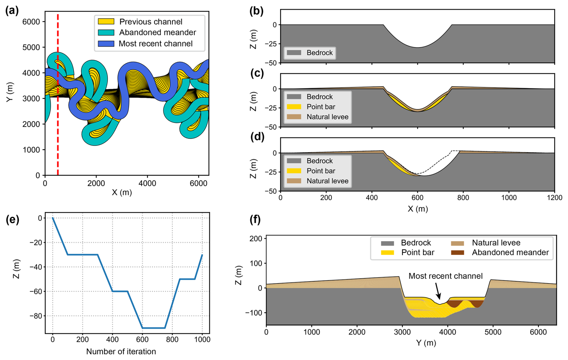
Figure 4 Submarine canyon modeling based on the open-source package meanderpy (Sylvester, 2021). (a) Lateral migration of a submarine channel. (b) Channel erosion and (c) deposition of point bars and natural levees. (d) The channel migrates toward the outer bend and erodes parts of the sediments. (e) Vertical component of the channel trajectory during the migration process, which is modified from Sylvester et al. (2011), showing an initial channel incision and a later aggradation. (f) The cross-section of the submarine canyon at the red dashed line in (a), showing a prominent erosional surface, the internal sediments, and wedge-like natural levees after 1000 iterations of channel migration.

To model the erosional surface and internal layered sediments of a submarine canyon, we adopt a modeling method based on submarine channel trajectories (Sylvester et al., 2011), which is also implemented in meanderpy. The modeling process is illustrated in Fig. 4. The model first simulates the lateral migration of a submarine channel (Fig. 4a). At each iteration during the migration process, a parabolic function (Eq. 1) is used to define the surface of channel erosion (Fig. 4b), which is followed by deposition of point bars and natural levees (Fig. 4c). Point bars are accumulated sediments on the inner bends of the channel, where the flow velocity is lower. Their top surface is defined using a combination of parabolic and Gaussian functions (Eqs. 2 and 3). For the convenience of modeling, point bars are created on both inner and outer bends, where those on the outer bends will be subsequently eroded. Natural levees are structures that form along the sides of a submarine channel when the turbidity currents overflow the channel banks. They typically exhibit a wedge-like shape because the turbidity current loses energy and sediments as it moves away from the channel margins. The thickness of the natural levee is defined as

$$\begin{array}{}\text{(5)}& T\left(x\right)=\left\{\begin{array}{ll}\frac{T_{\text{max}}}{W_{\mathrm{l}}}\left(x-\frac{W_{\mathrm{c}}-W_{\mathrm{l}}}{\mathrm{2}}\right),& x\ge W_{\mathrm{c}}\\ T_{\text{max}},& x<W_{\mathrm{c}}\end{array}\right.,\end{array}$$

where x denotes the distance to the channel centerline, T_max is the maximum thickness of the levee, W_l is the levee width, and W_c is the channel width. After the deposition of point bars and natural levees, the channel will migrate toward its outer bends and erode parts of these sediments (Fig. 4d). The erosion and deposition processes repeat until the channel migration ends. In the meantime, during lateral migration, the channel also experiences vertical incision and aggradation (Fig. 4e). When the channel migration ends, a submarine canyon will be created, along with wedge-like outer levees and internal layered sediments. The internal sediments consist of interbedded layers of point bars and inner levees, as well as abandoned meanders (Fig. 4f). To create diverse forms of submarine canyons, we use a random set of modeling parameters within reasonable ranges (see Table A1). Some of the submarine canyon models are demonstrated in Fig. 5c.

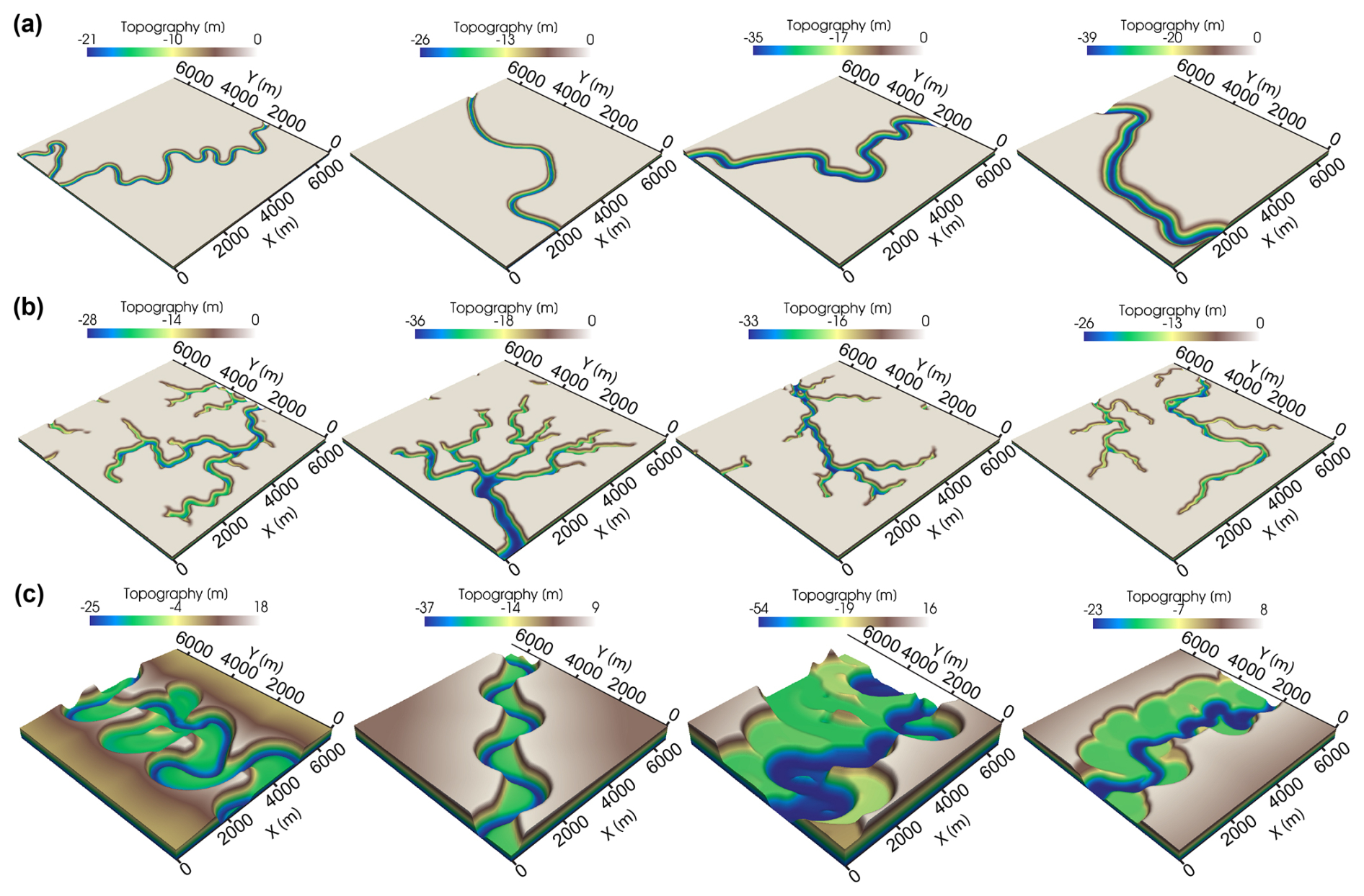
Figure 5 Diverse topographic models of (a) meandering channels, (b) tributary channel networks, and (c) submarine canyons.

2.4 Seismic volume simulation

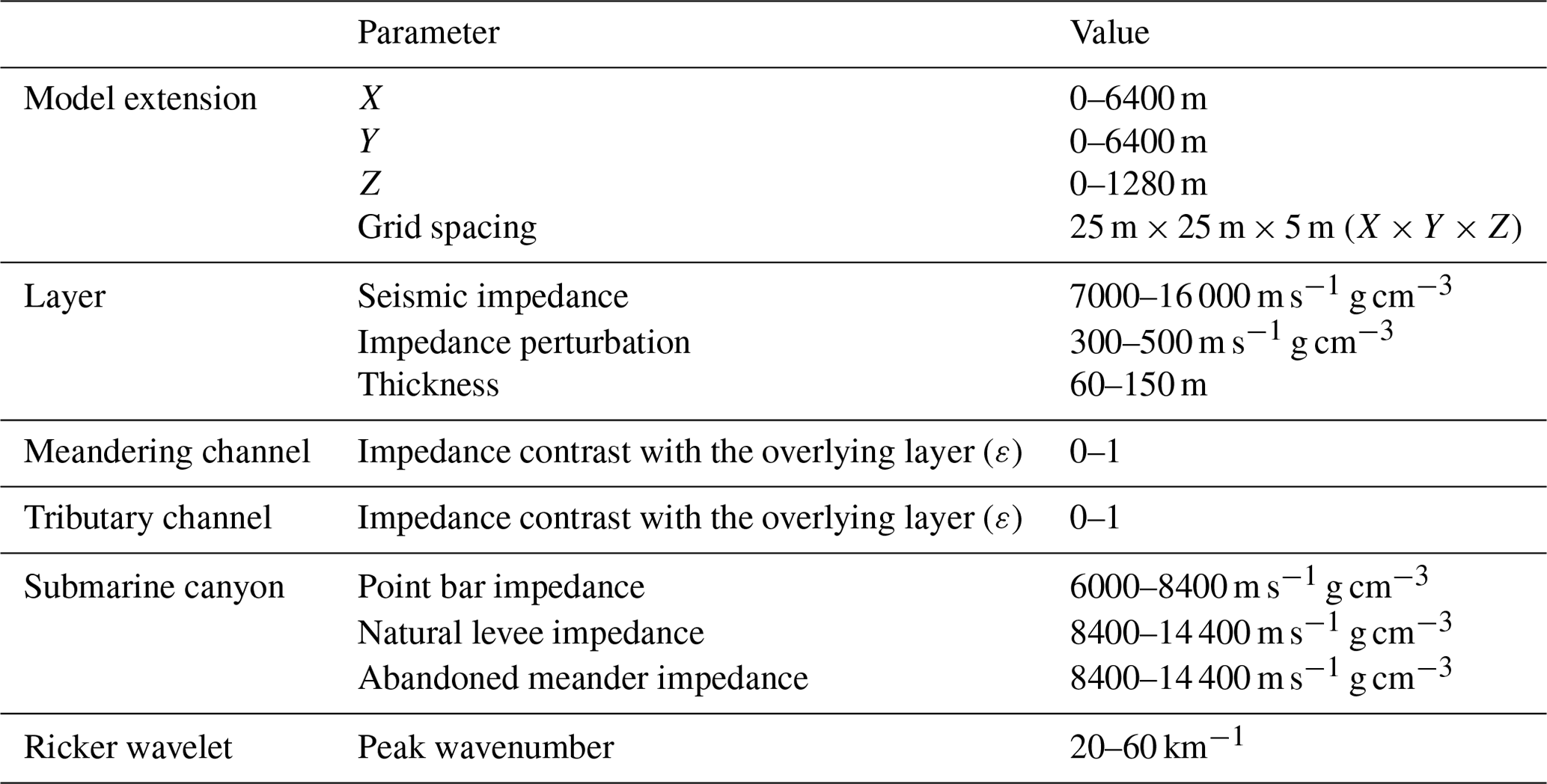
After constructing over 10 000 channel topographic models covering meandering channels, tributary channel networks, and submarine canyons, we proceed to create synthetic seismic volumes based on these models. The first step is to define the seismic impedance, which is a crucial parameter for simulating seismic events. In seismic exploration, seismic waves from an artificial source travel through the subsurface rock mass, and part of the waves will be reflected back to the surface at the boundaries of two geologic layers with a contrast in seismic impedance. The reflected seismic waves will form seismic events, which reflect the geometry of layer boundaries. The amplitudes of the seismic events are related to the contrast in seismic impedance between two layers. We start by generating 3D seismic impedance models with horizontal layers. In each layer, we add some minor random perturbations to the impedance to make it more realistic. Details of the configuration of the impedance model are listed in Table D1. The channel topographic models are then placed at the layer boundaries and the seismic impedance of the channel is defined according to the channel type.

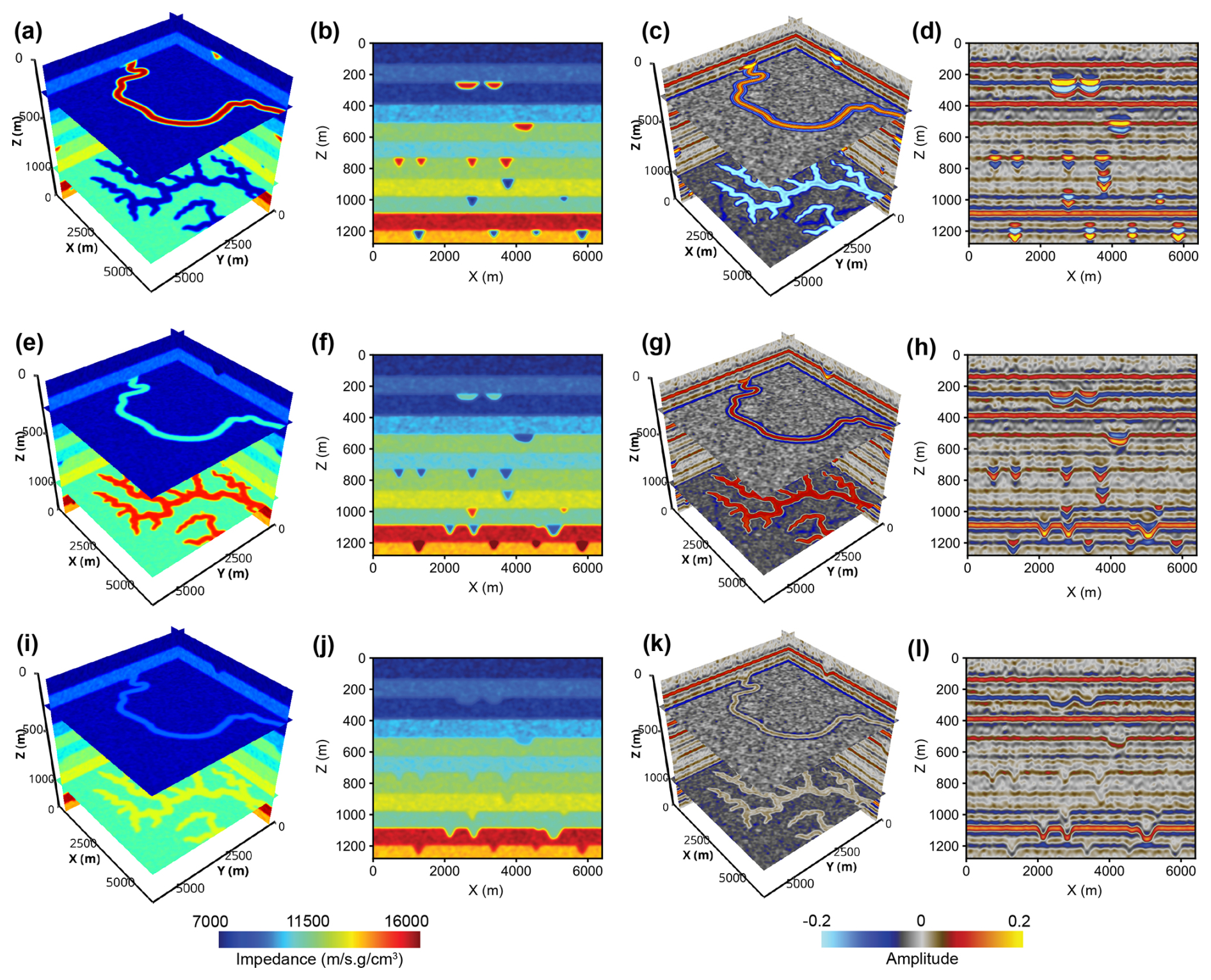
Figure 6 Seismic impedance and amplitude volumes containing meandering channels and tributary channel networks, showing different levels of impedance contrast between channels and their overlying layers. (a) to (d) correspond to channels with a high impedance contrast with their covering layers, (f) to (h) correspond to channels with a low impedance contrast, and (i) to (l) correspond to channels with no impedance contrast.

For meandering and tributary channels, we fill them with a relatively uniform impedance with some minor perturbations (approximately 100 m s⁻¹ g cm⁻³). The average impedance of the channel is determined by a parameter ε, which is defined as the impedance contrast between the channel and its overlying layer:

$$\begin{array}{}\text{(6)}& \mathit{\epsilon }={\displaystyle \frac{|Z_f-Z_u|}{Z_u}},\end{array}$$

where Z_f and Z_u denotes the impedance of the channel and its overlying layer, respectively. The value of ε varies between 0 and 1. ε=1 indicates the highest impedance contrast between the channel and its overlying layer, and ε=0 indicates equal impedance between the channel and its overlying layer. Figure 6a and b demonstrate the horizontal and vertical slices of a 3D impedance model, which consists of meandering and tributary channels with a high impedance contrast (ε=1). The impedance model is then used to calculate seismic reflectivity using the following equation:

$$\begin{array}{}\text{(7)}& R_i={\displaystyle \frac{Z_{i+\mathrm{1}}-Z_i}{Z_{i+\mathrm{1}}+Z_i}},i=\mathrm{1},\mathrm{2},\mathrm{\dots },N-\mathrm{1},\end{array}$$

where the subscript i denotes the ith point in the vertical (depth) direction of the model and N denotes the total number of points in the vertical direction. The reflectivity model is then convolved with a Ricker wavelet (see Fig. 8a and b for examples), which is commonly used to create synthetic seismic data. The mathematical expression of a Ricker wavelet in the depth domain is

$$\begin{array}{}\text{(8)}& f\left(s\right)=\left(\mathrm{1}-\mathrm{2}{\mathit{\pi }}^{\mathrm{2}}{k}_m^{\mathrm{2}}{s}^{\mathrm{2}}\right){\mathrm{e}}^{-{\mathit{\pi }}^{\mathrm{2}}{k}_m^{\mathrm{2}}{s}^{\mathrm{2}}},\end{array}$$

where s denotes the distance and k_m denotes the peak wavenumber of the wavelet. Figure 6c shows the seismic volume with a high impedance contrast between the channel and its overlying layer. The channels exhibit strong seismic amplitudes, as shown in Fig. 6d. As ε decreases to 0.2, the impedance contrast between the channel and its overlying layer becomes lower, as shown in Fig. 6e and f. The channel shows reduced seismic amplitude (Fig. 6g), appearing as infilling characteristics on the seismic profile (Fig. 6h). When ε=0, the impedance of the channel will be the same as that of its overlying layer (Fig. 6i and j). As a result, the channels show no internal seismic reflections except along their boundaries (Fig. 6k), forming U- or V-shaped reflection patterns on the seismic profile (Fig. 6l).

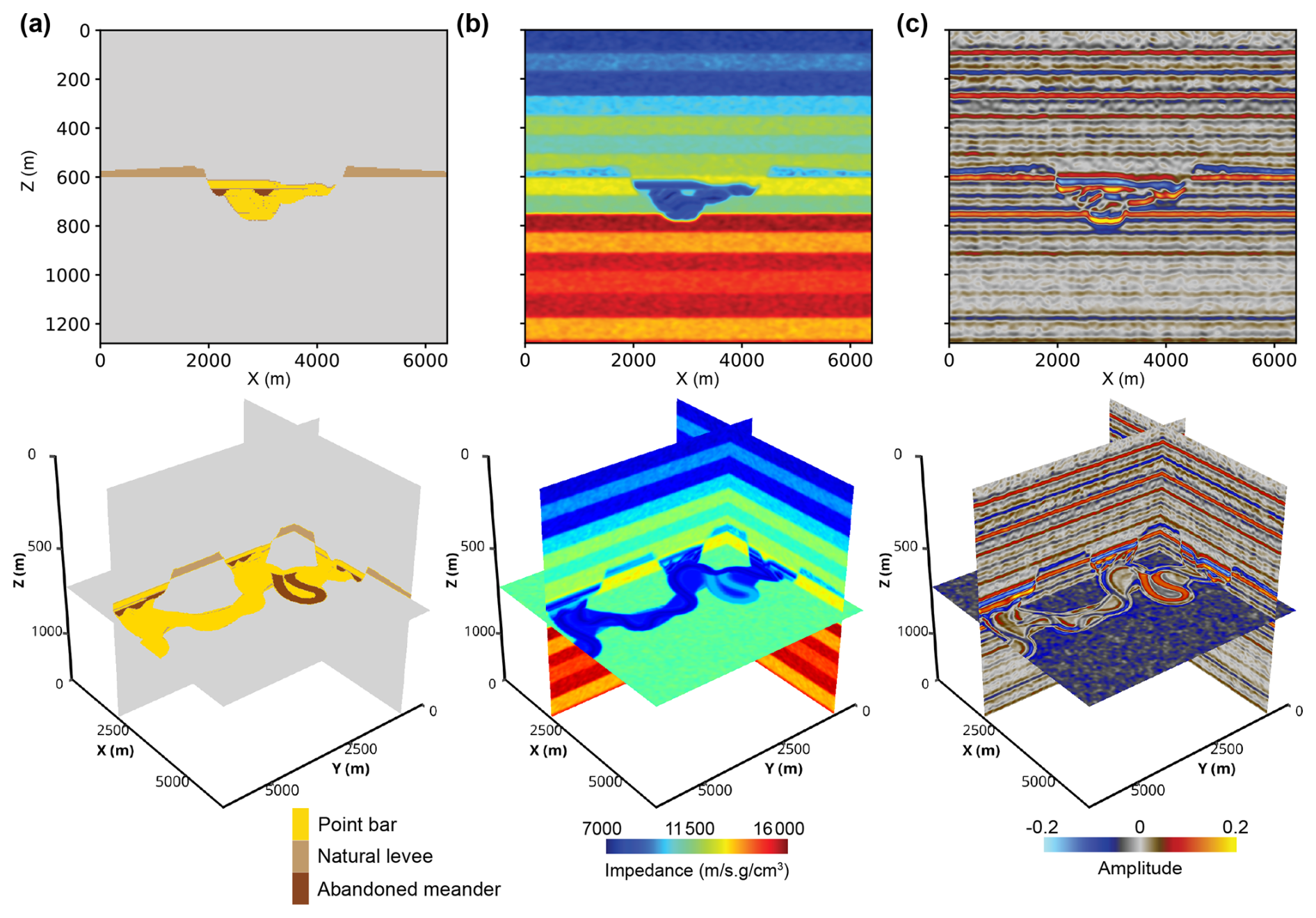
Figure 7 (a) Sedimentary facies, (b) seismic impedance, and (c) seismic amplitude of a submarine canyon.

The impedance of a submarine canyon is determined based on its sedimentary facies. Figure 7a shows the sedimentary facies of a submarine canyon, including point bar, natural levee, and abandoned meander. As shown in Fig. 7b, point bars are assumed to be sand-rich and are assigned a lower seismic impedance, whereas natural levees and abandoned meanders are considered mud-rich and are assigned a higher impedance. The impedance range for each sedimentary facies is listed in Table D1. The impedance contrasts between adjacent layers within the point bars result in internal seismic reflections that appear as layered patterns on seismic profiles and meander-belt-like patterns on horizontal slices, as shown in Fig. 7c. Minor impedance perturbations (±100 m s⁻¹ g cm⁻³) also exist within each sedimentary facies.

In the current impedance model, all the channels and layers are modeled as horizontal. However, in real-world settings, channels and layers often undergo structural deformation (e.g., folding and faulting), which are commonly observed in many field seismic volumes. To increase the diversity and realism of synthetic seismic volumes, we introduce inclination, folds, and faults into the impedance model following the workflow proposed by Wu et al. (2020a). An example of the resulting impedance model with structural deformation is shown in Fig. 8c. Another way to increase the diversity of the synthetic seismic volumes is to use wavelets with various peak wavenumbers. This consideration is also important, as the peak wavenumber of seismic reflections from the channel can vary significantly in field seismic volumes, depending on various factors, such as the absorption effects of subsurface media and the characteristics of the seismic source (Yilmaz, 2001). Figure 8 shows two synthetic seismic profiles generated using different wavelets but the same impedance model. A wavelet with a smaller peak wavenumber (Fig. 8a) results in a low-resolution seismic profile with broad seismic events (Fig. 8d), where some thin layers within the submarine canyon at the bottom of the profile are difficult to distinguish. In contrast, using a wavelet with a larger peak wavenumber (Fig. 8b) produces a high-resolution seismic profile (Fig. 8e), in which those thin layers within the submarine canyon become clearly discernible. The peak wavenumber ranges of the Ricker wavelets used to generate the synthetic seismic volumes are listed in Table D1.

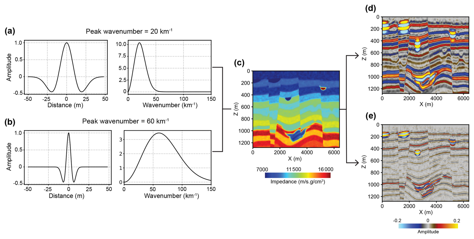
Figure 8 Synthetic seismic profiles with different wavelets computed from the same seismic impedance model. (a) A small-wavenumber Ricker wavelet with a peak wavenumber of 20 km⁻¹ (corresponding to a peak frequency of 20 Hz) in depth and wavenumber domain. (b) A large-wavenumber Ricker wavelet with a peak frequency of 60 km⁻¹ (corresponding to a peak frequency of 60 Hz) in depth and wavenumber domain. (c) Seismic impedance model. (d) Low-resolution seismic profile generated by using the small-wavenumber wavelet. (e) High-resolution seismic profile generated by using the large-wavenumber wavelet.

3 Results

Using the proposed workflow, we constructed the cigChannel dataset (Wang et al., 2024, https://doi.org/10.5281/zenodo.10791151), which consists of 1600 synthetic seismic volumes with over 10 000 labeled paleochannels. Each seismic volume has a size of $\mathrm{256}\times \mathrm{256}\times \mathrm{256}$ samples. This dataset is organized into four subsets, corresponding to different channel types: meandering channels, tributary channel networks, submarine canyons, and assorted channels. Examples of seismic volumes and paleochannel labels in these four subsets are demonstrated in Fig. 9. In addition to the seismic volumes, the cigChannel dataset provides the corresponding seismic impedance models, as illustrated in Fig. S1 of the Supplement. Furthermore, the submarine canyon subset provides sedimentary facies volumes corresponding to the submarine canyon, with illustrative examples shown in Fig. S2 of the Supplement. A detailed breakdown of the dataset's components is presented in Table B1.

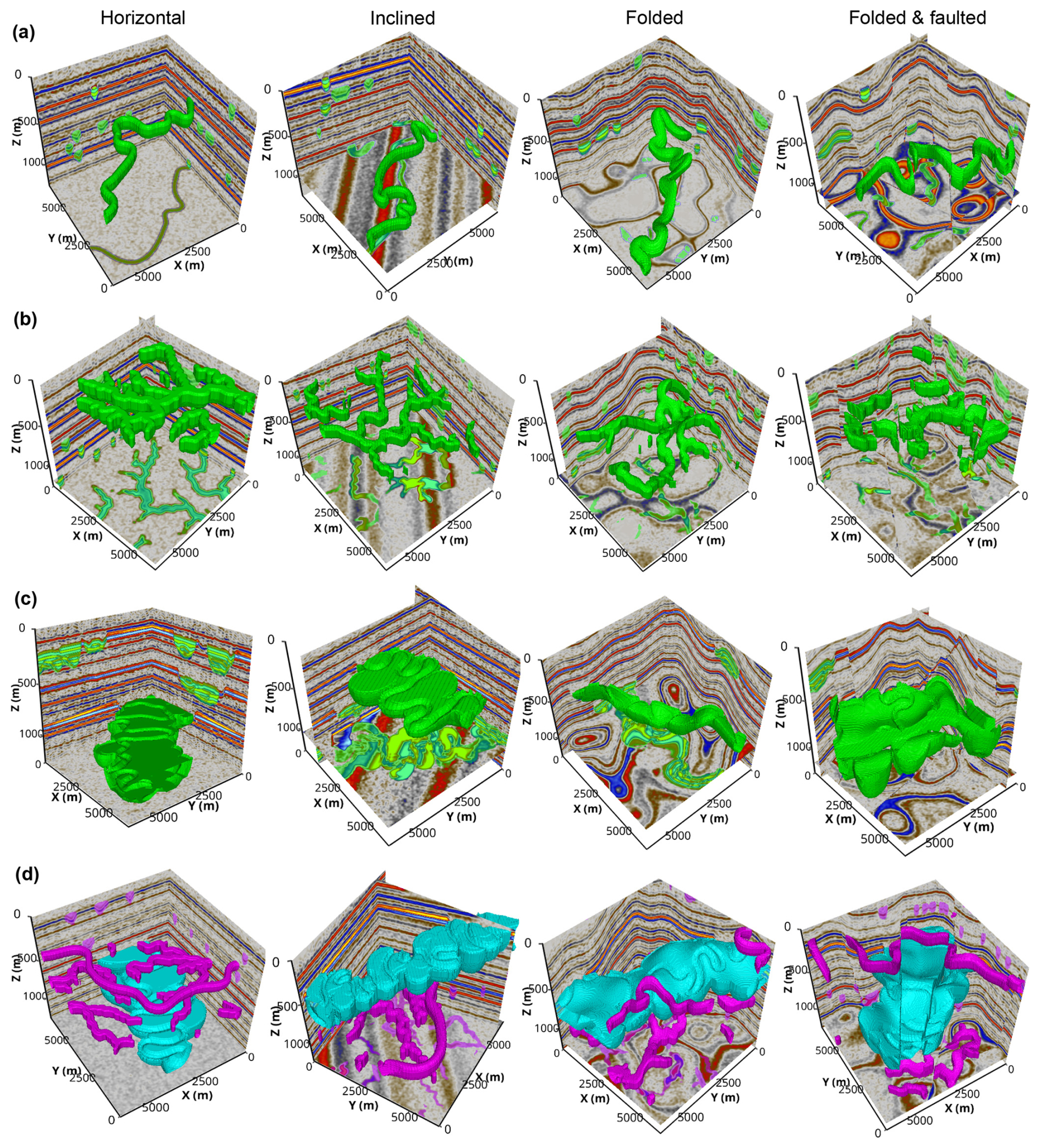
Figure 9 Synthetic seismic volumes and paleochannel labels in the (a) meandering channel, (b) tributary channel network, (c) submarine canyon, and (d) assorted channel subsets of the cigChannel dataset, showing various types of structure. The first three subsets provide binary class labels to distinguish between channels and the background (i.e., the non-channel areas), while the assorted channel subset provides multi-class labels to distinguish between terrestrial channels, submarine canyons, and the background.

For training deep learning models to identify specific types of channel, the subsets of meandering channels, tributary channel networks, and submarine canyons each provide 400 seismic volumes containing only the corresponding type of channel. Each subset provides binary class labels, where 0 denotes non-channel areas and 1 denotes channels. As shown in Fig. 9, each subset contains seismic volumes with horizontal, inclined, folded, and faulted structures, aiming to facilitate the training of deep learning models to identify channels associated with various structural styles. These structures are randomly generated to introduce variability into the seismic volumes. Since submarine canyons are generally wider and deeper than terrestrial channels (Normark et al., 2003; Kolla et al., 2007; Covault et al., 2021), this characteristic is reflected in the cigChannel dataset by generating submarine canyons that are larger than meandering and tributary channels.

The assorted channel subset also has 400 seismic volumes. Each seismic volume contains multiple terrestrial channels (including meandering channels and tributary channel networks) and one submarine canyon. This subset provides multi-class labels of non-channel areas, terrestrial channels, and submarine canyons, as shown in Fig. 9d. They are denoted by 0, 1, and 2 in the label volume, respectively. The reason for simulating multiple terrestrial channels but only one submarine canyon in a single seismic volume is to balance their voxel amounts, since a model trained on an imbalanced dataset performs poorly on the minority class (i.e., the class-imbalance problem). However, there is still a huge gap in voxel amounts between channels and non-channel areas. This gap exists in all four subsets. Therefore, we suggest the adoption of strategies for addressing the class-imbalance problem when using the cigChannel dataset to train a deep learning model, such as employing the class-balanced cross-entropy loss function (Xie and Tu, 2015).

4 Applications

Three U-Nets are trained on the subsets of meandering channels, tributary channel networks, and submarine canyons, respectively, which are then applied to identify paleochannels in field seismic volumes. The U-Net architecture used in this study is shown in Fig. 10, where the number of convolutional layers and feature maps is reduced from the original design in Ronneberger et al. (2015) to reduce memory usage and computational cost. The network's input is a seismic volume of $\mathrm{224}\times \mathrm{224}\times \mathrm{224}$ samples, which is cropped from the original volume of $\mathrm{256}\times \mathrm{256}\times \mathrm{256}$ samples due to the memory limit of the GPU. Each seismic volume is normalized using the mean-variance normalization method, and Gaussian random noise is added to the synthetic seismic volume to make the training process more robust and reduce the tendency toward overfitting. The added noise is zero-mean and its standard deviation is determined according to the expected signal-to-noise ratio (SNR) of the noisy seismic volume. We set the SNR of each seismic volume to vary between 5 and 10 dB; this is a reasonable range for field seismic volumes (Zhang et al., 2017; Wu et al., 2021). The noisy seismic volume goes through the contracting and expansive path of the U-Net for feature extraction. The final output layer of the network is a $\mathrm{3}\times \mathrm{3}\times \mathrm{3}$ convolutional layer followed by a sigmoid activation, which maps the extracted feature into channel probabilities between 0 and 1. We binarize the channel probabilities using a threshold of 0.5 in order to obtain a binary segmentation of channels and non-channel areas.

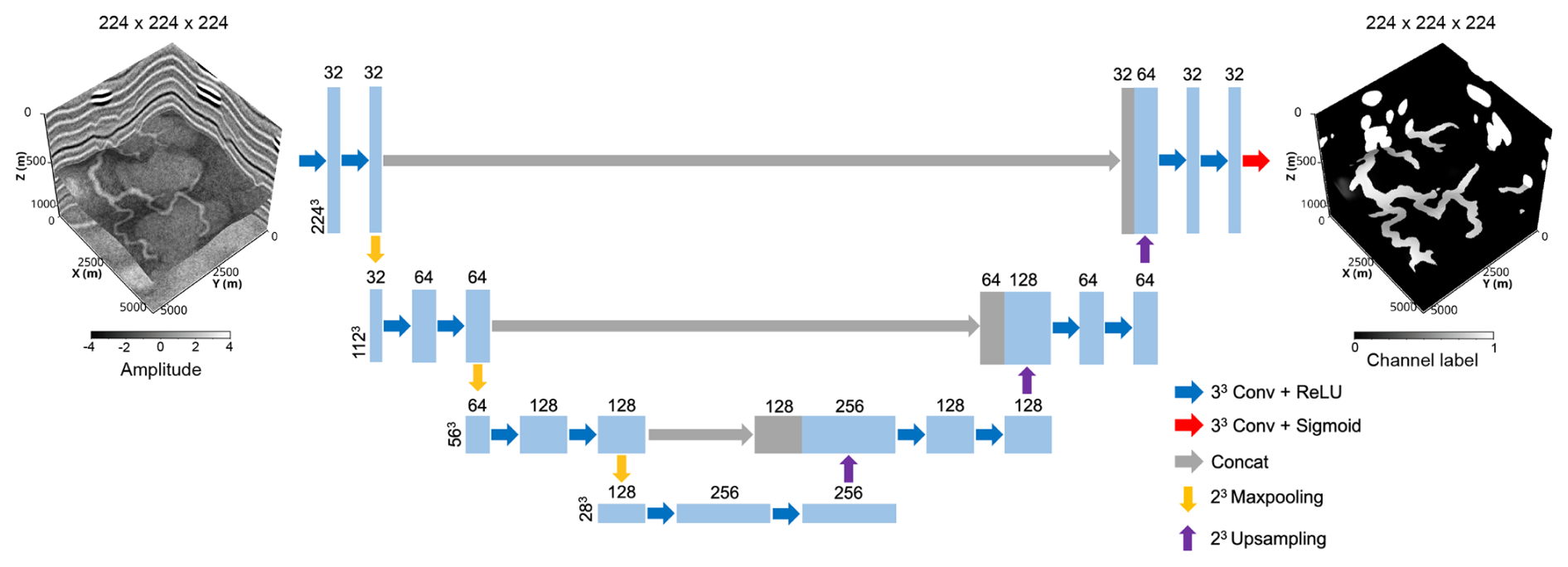
Figure 10 A simplified U-Net for identifying paleochannels in seismic volumes. The inputs of the U-Net are seismic volumes and the outputs are channel probabilities between 0 and 1.

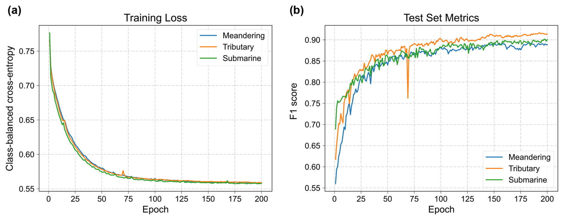
Figure 11 Training progress of the U-Net on the subsets of meandering channels, tributary channel networks, and submarine canyons, showing (a) the training loss (class-balanced cross-entropy) and (b) the F₁ score on the test set over epochs.

To evaluate the training performance, each subset is divided into training and test sets. The training and test sets contain 70 % and 30 % of the total samples, respectively. The class-balanced cross-entropy is used as the loss function, considering the huge gap in voxel amounts between channels and non-channel areas. The F₁ score is used as a metric to evaluate the network's performance on the test set. We use the Adam method (Kingma, 2014) to optimize the network's parameters and set the learning rate to be 0.0001. As shown in Fig. 11, the training loss of each network converges after 200 epochs, and the F₁ scores of the test sets gradually increase to around 0.9. The networks from the final epoch are used to identify paleochannels in field seismic volumes.

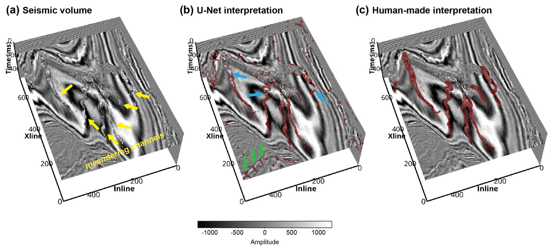
Figure 12 (a) Seismic volume from the Parihaka seismic survey (courtesy of New Zealand Crown Minerals), showing multiple meandering channels (indicated by the yellow arrows). (b) Channel interpretation result of the U-Net trained on the subset of meandering channels. The blue arrows indicate channel areas that could not be identified, and the green arrows indicate false positive channel identification results. (c) Human-made channel interpretation result.

The first U-Net is trained on the meandering channel subset and applied to a volume from the Parihaka seismic survey. As shown in Fig. 12a, the seismic volume reveals several meandering channels feeding into a larger channel (maybe a submarine canyon). The channel identification result of the U-Net is shown in Fig. 12b, and has a F₁ score of 0.52 when compared with the human-made channel interpretation (Fig. 12c). Some channel areas with significant variations in seismic amplitude or where the channel width suddenly increases are not correctly identified, as indicated by the blue arrows in Fig. 12b. This is probably because each meandering channel in the training set has a fixed channel width, and the seismic amplitude within each channel is relatively uniform. Moreover, there are many false positive channel identification results, as indicated by the green arrows in Fig. 12b, which might be local structural deformations that resemble the feature of a U- or V-shaped channel.

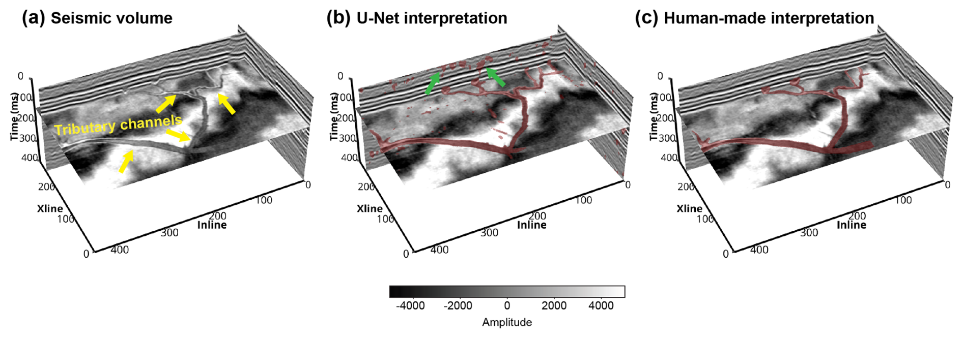
Figure 13 (a) Seismic volume from an anonymous seismic survey (denoted as NW seismic survey), showing a tributary channel network (indicated by the yellow arrows) with V-shaped channel cross-sections. (b) Channel interpretation result of the U-Net trained on the subset of tributary channel networks. Some false positive channel interpretation results are indicated by the green arrows. (c) Human-made channel interpretation result.

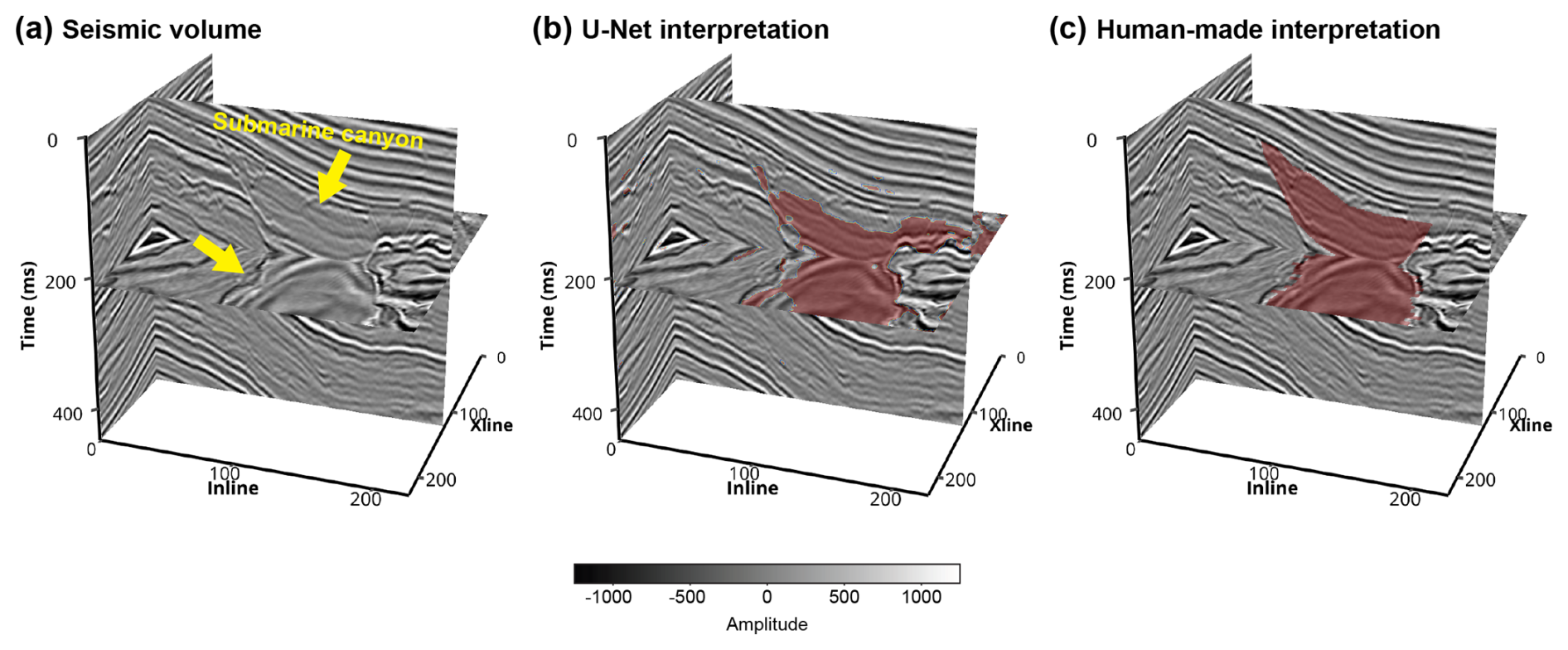
Figure 14 (a) A field seismic volume from the Parihaka seismic survey (courtesy of New Zealand Crown Minerals), showing a submarine canyon (indicated by the yellow arrows). (b) Channel interpretation result of the U-Net trained on the subset of submarine canyon. (c) Human-made channel interpretation result.

The second U-Net is trained on the tributary channel network subset and applied to a volume from an anonymous seismic survey (denoted as NW seismic survey hereafter). As demonstrated in Fig. 13a, this seismic volume shows a tributary channel network with V-shaped channel cross-sections. Seismic amplitudes within the channel are relatively homogeneous, indicating a relatively uniform seismic impedance within the channel, as we designed in our data generation workflow. The channel identification result of the U-Net is demonstrated in Fig. 13b, showing that most of the channels are correctly identified. However, there are still a number of small-scale structural deformations that are mistakenly identified as channels, as indicated by the green arrows in Fig. 13b. The F₁ score between the U-Net and human-made interpretation result (Fig. 13c) is 0.73.

The last U-Net is trained on the submarine canyon subset and applied to another volume from the Parihaka seismic survey. As demonstrated in Fig. 14a, a submarine canyon characterized by a prominent erosional surface is observed in the seismic volume. It has a relatively low seismic amplitude compared with that of its surrounding layers, indicating a low discrepancy in seismic impedance within the canyon. However, some layered structures are still visible within the canyon. Figure 14b demonstrates the channel identification result of the U-Net. Most areas of the submarine canyon are correctly identified but the U-Net cannot delineate the canyon boundary accurately. The F₁ score between the U-Net and human-made interpretation result (Fig. 14c) is 0.63.

5 Discussion

5.1 Plausibility of the synthetic seismic volumes

While the cigChannel dataset provides various samples for training deep learning models to identify paleochannels in seismic volumes, the plausibility of the synthetic seismic volume remains uncertain. Several simplifications are applied to reduce computational costs during the generation of synthetic seismic volumes. For instance, the configuration of seismic impedance models ignores the variability within layers and channel facies. However, this variability is ubiquitous in the subsurface. Moreover, the forward seismic modeling uses the simplest 1D convolution between seismic (P-wave) impedance and Ricker wavelet. It disregards many aspects of wave propagation in the subsurface, including the contribution of shear waves, separate contributions from P-wave velocity and density, and multi-path reflection. These simplifications reduce the realism of synthetic seismic volumes. It is questionable whether the synthetic seismic volumes can capture the patterns in the field seismic volumes.

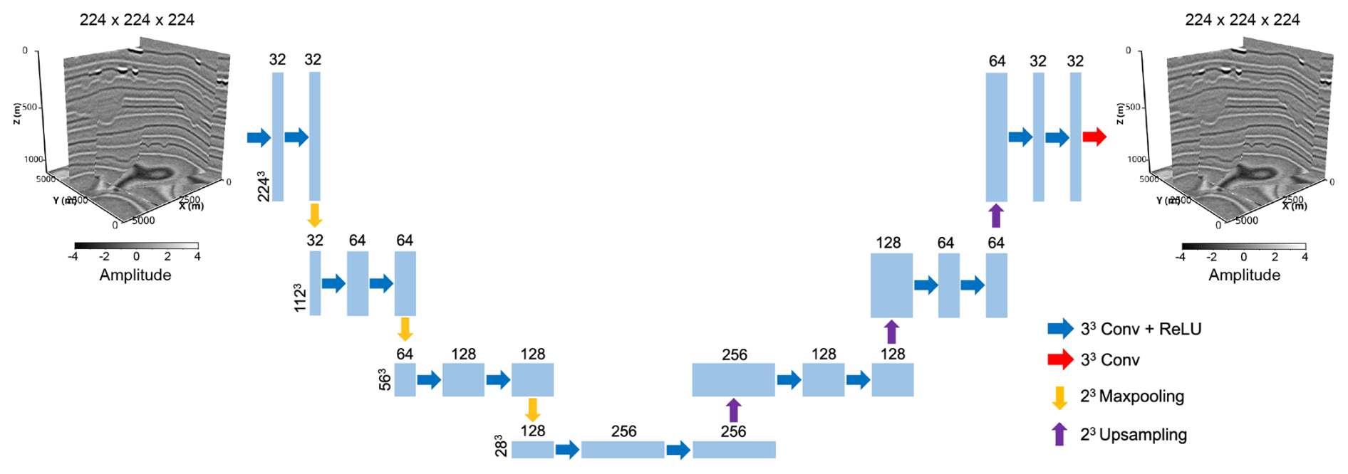
Figure 15 U-Net-based autoencoder architecture for reconstructing seismic volumes. Compared with the U-Net architecture used for paleochannel identification, the skip connections are removed, and the final layer is a $\mathrm{3}\times \mathrm{3}\times \mathrm{3}$ convolutional layer without sigmoid activation. The inputs of the autoencoder are the original seismic volumes and the outputs are their reconstruction results.

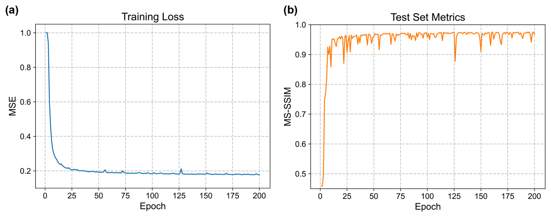
Figure 16 Training progress of the U-Net-based autoencoder, showing (a) training loss (mean squared error) and (b) multi-scale structural similarity (MS-SSIM) on the test set over epochs.

To answer this question quantitatively, we use the synthetic seismic volumes in the cigChannel dataset to train an autoencoder to reconstruct seismic volumes. If this autoencoder can reconstruct the field seismic volumes as well as the synthetic ones, then the synthetic seismic volumes are plausible and representative enough of field seismic volumes. Otherwise, room for improvement is indicated. To construct training and test sets, we randomly choose 70 samples for training and 30 samples for testing from each subset. That makes a total number of 280 training samples and 120 test samples. The architecture of the autoencoder is adapted from the U-Net used for identifying paleochannels. As shown in Fig. 15, we remove all the skip connections from the U-Net and the sigmoid activation from the final convolutional layer. Each synthetic seismic volume is cropped to a size of $\mathrm{224}\times \mathrm{224}\times \mathrm{224}$ samples. These samples will serve as both inputs and labels to train the autoencoder. The seismic volumes (both synthetic and field ones) will be normalized and zero-mean Gaussian random noise will be added to the synthetic seismic volume. The standard deviation of the noise is determined according to the expected SNR of the noisy seismic volume, which is set to vary between 5 and 10 dB. During the training process, the mean squared error (MSE) between the original and reconstructed seismic volumes will be calculated as the training loss, and the multi-scale structural similarity (MS-SSIM) will be used as a metric to evaluate the network's generalization performance on the test set.

Figure 16 shows the evolution of training loss and test set metrics over the training epochs. The training loss decreases rapidly in the first 25 epochs and reaches full convergence after 200 epochs. Meanwhile, the reconstruction of seismic volumes in the test set achieves an average MS-SSIM of 0.96, in spite of some minor fluctuations. The reconstruction of a synthetic seismic volume from the test set is demonstrated in Fig. 17a. Seismic events, including those related to the paleochannels are mostly reconstructed. However, as shown in the residual volume, random noise and some weak seismic reflections within geologic layers (i.e., between seismic events) are not fully recovered. The reconstruction results of the three field seismic volumes with meandering channels, a tributary channel network, and a submarine canyon are respectively demonstrated in Fig. 17b, c, and d. The general patterns (i.e., geometries, relative seismic amplitudes) of the seismic events and paleochannels have been successfully reconstructed. However, we can see from the residual volumes that many detailed seismic reflections related to the geologic layers and paleochannels have not been recovered, especially for the seismic volumes from the Parihaka survey (Fig. 17b and c). Table 1 lists the metrics of the autoencoder for reconstructing the synthetic and field seismic volumes shown in Fig. 17. The reconstruction of the Parihaka seismic volumes (Fig. 17b and d) is less accurate, compared with that of the synthetic seismic volume (Fig. 17a). However, the autoencoder is capable of reconstructing the NW seismic volume (Fig. 17c) with a quality comparable to that of the synthetic seismic volume.

Table 1 Metrics of the autoencoder for reconstructing synthetic and field seismic volumes.

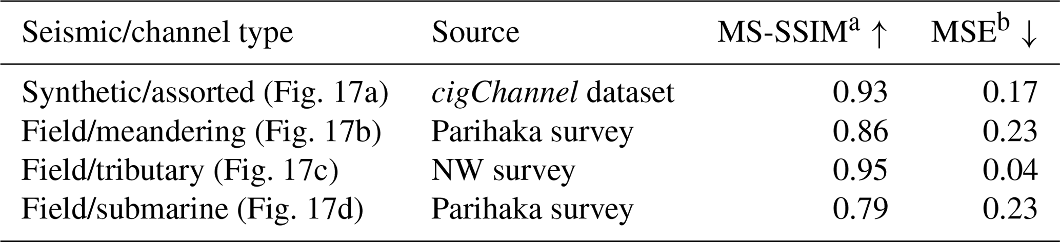
^a MS-SSIM: Multi-scale structural similarity.
^b MSE: Mean squared error.

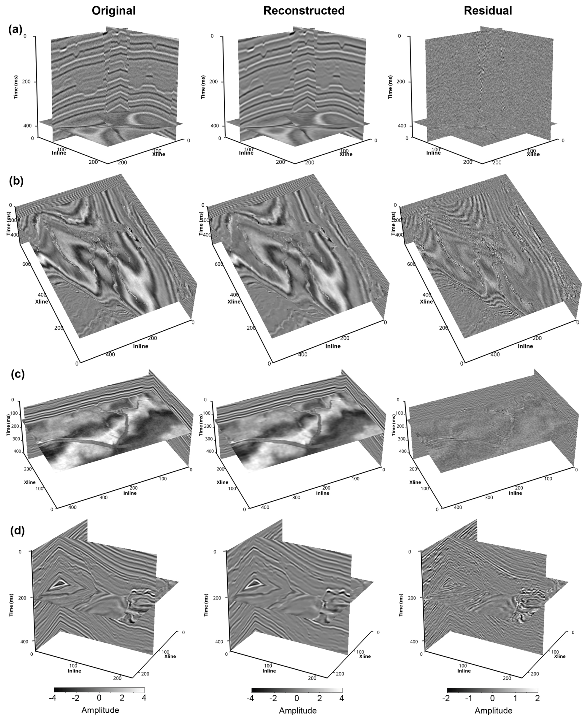
Figure 17 The original, reconstructed, and residual volumes of synthetic and field seismic data. (a) Synthetic seismic volume with assorted channels. (b–d) Field seismic volumes with (b) meandering channels, (c) a tributary channel network, and (d) a submarine canyon.

The difference in reconstruction performance on field seismic volumes is likely to be related to the variability in seismic data. Compared with the two Parihaka seismic volumes (Fig. 17b and d), the NW seismic volume (Fig. 17c) has less variation in seismic amplitude along seismic events and the seismic amplitude within paleochannels is relatively uniform. These characteristics are similar to the synthetic seismic volumes and therefore the autoencoder can reconstruct the NW seismic volume as effectively as the synthetic ones. In conclusion, the synthetic seismic volumes have captured general patterns in field seismic data, such as the geometries of structures and paleochannels. However, they cannot capture the detailed variations in seismic data that are related to wave propagation and changes in rock properties. This may lead to generalization issues for deep learning models trained on this dataset when applied to field seismic volumes with significant variability. Applying more realistic seismic forward modeling methods, such as full-waveform modeling, and considering the variations in rock properties within geologic layers and paleochannel facies could help improve the plausibility of the synthetic seismic volumes.

5.2 Limitations of the dataset

Although the application of the cigChannel dataset has shown the capability of training deep learning models to identify paleochannels in field seismic volumes, there are several limitations of this dataset that users should be aware of. The first one lies in the diversity of terrestrial channel and submarine canyon models. The widths of terrestrial channels are set to be relatively small (≤500 m) in order to be more distinguishable from submarine canyons. However, much wider terrestrial channel systems (e.g., ≥1 km) have also been reported (Gibling, 2006), which could be comparable in size to a relatively narrow submarine canyon, such as the La Jolla canyon (Paull et al., 2013). Therefore, if the aim is to train a deep learning model to differentiate between terrestrial channels and submarine canyons, then the model trained on the assorted channel subset may face challenges when distinguishing small submarine canyons from large terrestrial channels. Moreover, as we mentioned, our modeling of submarine canyons aims to replicate the characteristics of the submarine channel–levee system, so requires enough fine-grained sediments to form levees. Relatively coarse-grained sediments (e.g., conglomeratic channel lag deposits) that correspond to a sandier depositional environment are not captured in our submarine canyon models. Consequently, deep learning models trained on the submarine canyon subset may struggle to accurately identify submarine canyons that contain a significant amount of coarse-grained sediments.

The second limitation concerns the realism of seismic impedance within channels. We assign a relatively uniform seismic impedance to terrestrial channels, introducing slight random perturbations to capture natural variability. The seismic impedance of these channels is determined based on a predefined contrast with the overlying layers. However, these simplifications reduce the realism of the impedance representation. In reality, terrestrial channel fills exhibit variations in facies and lithologies (Miall, 2014; Mueller and Pitlick, 2013), which can result in considerable seismic impedance heterogeneity. Although, under certain circumstances, this heterogeneity could be diminished, due to the relatively small size of terrestrial channels and the inherent limitations of seismic resolution, assigning a relatively uniform impedance to terrestrial channels limits the comprehensiveness of their seismic response. As a result, deep learning models trained on the subset of meandering channels or tributary channel networks may face challenges in accurately identifying channels that exhibit heterogeneous seismic amplitudes, such as the example shown in Fig. 12. Additionally, for submarine canyons, seismic impedance variations related to grain size distribution within sedimentary facies are not accounted for. The spatial transition from coarse-grained sediments in the channel thalweg to fine-grained sediments along the channel margins (Jobe et al., 2017) is not represented in our impedance models, which further limits the diversity and realism of the synthetic seismic volumes. Consequently, deep learning models trained on the submarine canyon subset may face generalization challenges when applied to identify submarine canyons in field seismic volumes.

The third limitation relates to the realism of non-channel areas in the synthetic seismic volumes. In addition to not fully capturing various characteristics of wave propagation due to the use of 1D convolution for seismic synthesis, the synthetic seismic volumes also lack structural diversity and stratigraphic variability. While folds and faults are included, their scales are enlarged to be comparable to the horizontal extent of the seismic volumes (i.e., 6.4 km). Small-scale (e.g., hundreds of meters) structural deformations, particularly those forming localized U- or V-shaped geometries, are not incorporated, despite their common occurrence in field seismic volumes. Consequently, deep learning models trained on our dataset may struggle to distinguish between small-scale concave structures and U- or V-shaped channels, potentially leading to false positive results. Moreover, each layer in the seismic impedance model is assigned a uniform thickness and a relatively consistent seismic impedance, resulting in a lack of stratigraphic variability in the synthetic seismic volumes. Given this limitation, it is not surprising that a deep learning model trained on our dataset may infer that the primary distinction between channel and non-channel areas is the presence of stratigraphic variability. This inference arises because, in the synthetic seismic volumes, channels – particularly submarine canyons – are the only structures exhibiting such variability. However, in field seismic volumes, stratigraphic variability is widespread among non-channel areas. Consequently, deep learning models trained on our dataset may produce false positives in non-channel areas with significant stratigraphic variability.

6 Code and data availability

The cigChannel dataset is available at https://doi.org/10.5281/zenodo.10791151 (Wang et al., 2024). The codes for dataset generation and the U-Net model used for paleochannel identification are available at https://github.com/wanggy-1/cigChannel (Wang, 2024). The three seismic volumes presented in the Applications section are available at https://drive.google.com/drive/folders/1owPqFv63Di1KKV9jdbn4vyidyG5l2wuR?usp=drive_link (Wang, 2025).

7 Conclusions

In this paper, we present a workflow for generating a large number of 3D synthetic seismic volumes containing paleochannels, along with their corresponding segmentation labels. Using this approach, we construct the cigChannel dataset, which comprises 1600 seismic volumes featuring three distinct types of paleochannel. This dataset is designed to address the scarcity of training data for deep-learning-based paleochannel identification in seismic volumes. Compared with previously used datasets (Pham et al., 2019, and Gao et al., 2021), the cigChannel dataset offers a more diverse and comprehensive collection of paleochannels. The effectiveness of this dataset is demonstrated through its application to three field seismic volumes, where three simplified U-Nets, trained on the cigChannel dataset, successfully identify paleochannels, with promising results. This highlights the feasibility of using synthetic data to train deep learning models for paleochannel identification, bridging the gap between limited field seismic volume annotations and the need for efficient and robust seismic paleochannel interpretation. Beyond providing a rich source of training samples for deep learning models, the cigChannel dataset and its generation workflow hold potential for advancing seismic modeling techniques and supporting educational applications. For example, rock physics models incorporating fluvial or turbiditic facies could be developed to evaluate new seismic modeling approaches, while the synthetic seismic volumes could serve as effective tools for demonstrating the influence of geological heterogeneities on seismic data. However, synthetic seismic volumes in the cigChannel dataset still lack the diversity and realism of field seismic volumes, primarily due to the simplifications of channel modeling, seismic impedance representation, and the synthesis of seismic volumes.

In the future, we aim to enhance our workflow to improve the realism and diversity of the generated seismic volumes. Terrestrial channels will be modeled using stratigraphic approaches to better capture sedimentary processes, thereby enhancing geological realism. The dataset will also be expanded to include a broader range of channel types, such as braided channels and deltaic systems, further increasing its diversity. To improve seismic impedance modeling, we plan to account for grain size distribution and its impact on impedance variations within channel sedimentary facies. Additionally, the current simplistic 1D convolution will be replaced with 3D convolution or full-waveform modeling to better capture the variability in seismic data. These advancements will enhance the geological realism and diversity of our dataset, ultimately improving its effectiveness for deep-learning-based seismic paleochannel interpretation.

Appendix A: Channel modeling parameters

(Gibling, 2006)(Gibling, 2006)(Donovan et al., 2021; Schook et al., 2017; Heo et al., 2009)(Chow, 1988)(Trigg et al., 2012)(Gibling, 2006)(Shumaker et al., 2018)(Shumaker et al., 2018)(Biscara et al., 2013)(Chow, 1988)(Allen et al., 2022)(Klaucke et al., 1998)(Englert et al., 2020)(Englert et al., 2020)

Table A1 Channel modeling parameters.

Appendix B: Components of the cigChannel dataset

Table B1 Components of the cigChannel dataset.

Appendix C: Demonstration codes of the dataset generation workflow

Listing C1 Demonstration codes of the dataset generation workflow.

Appendix D: Parameters of the seismic impedance model and Ricker wavelet

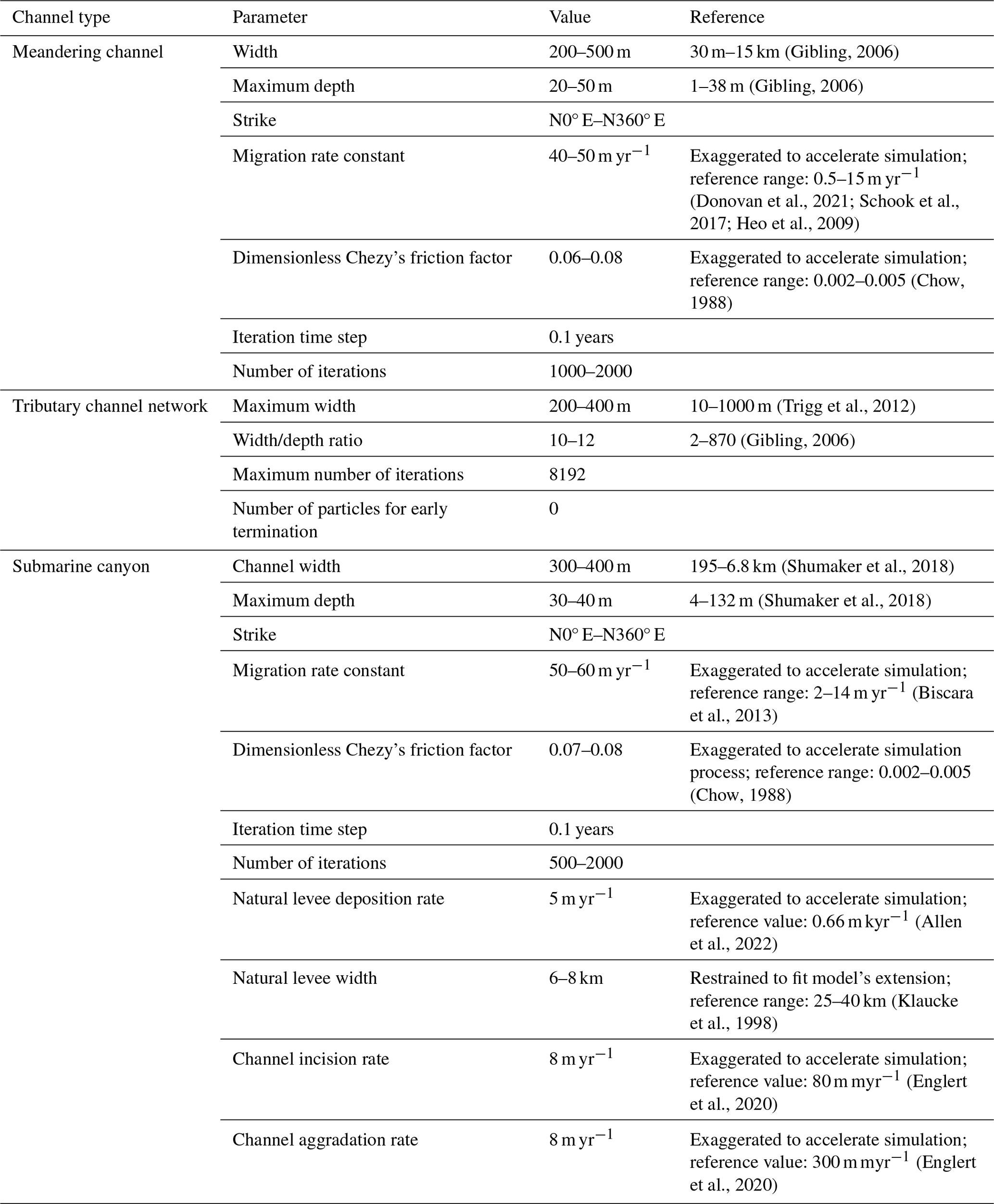
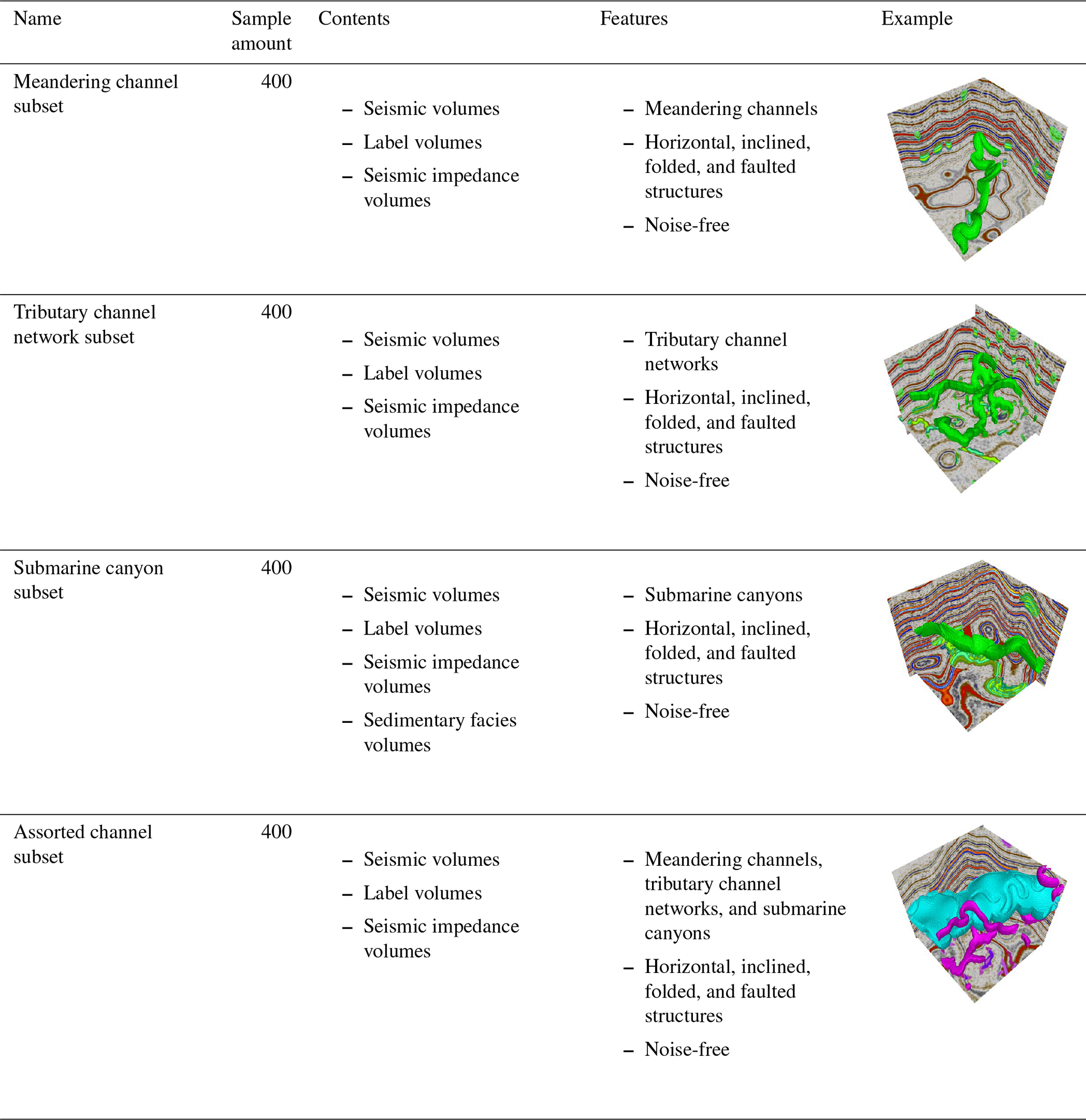
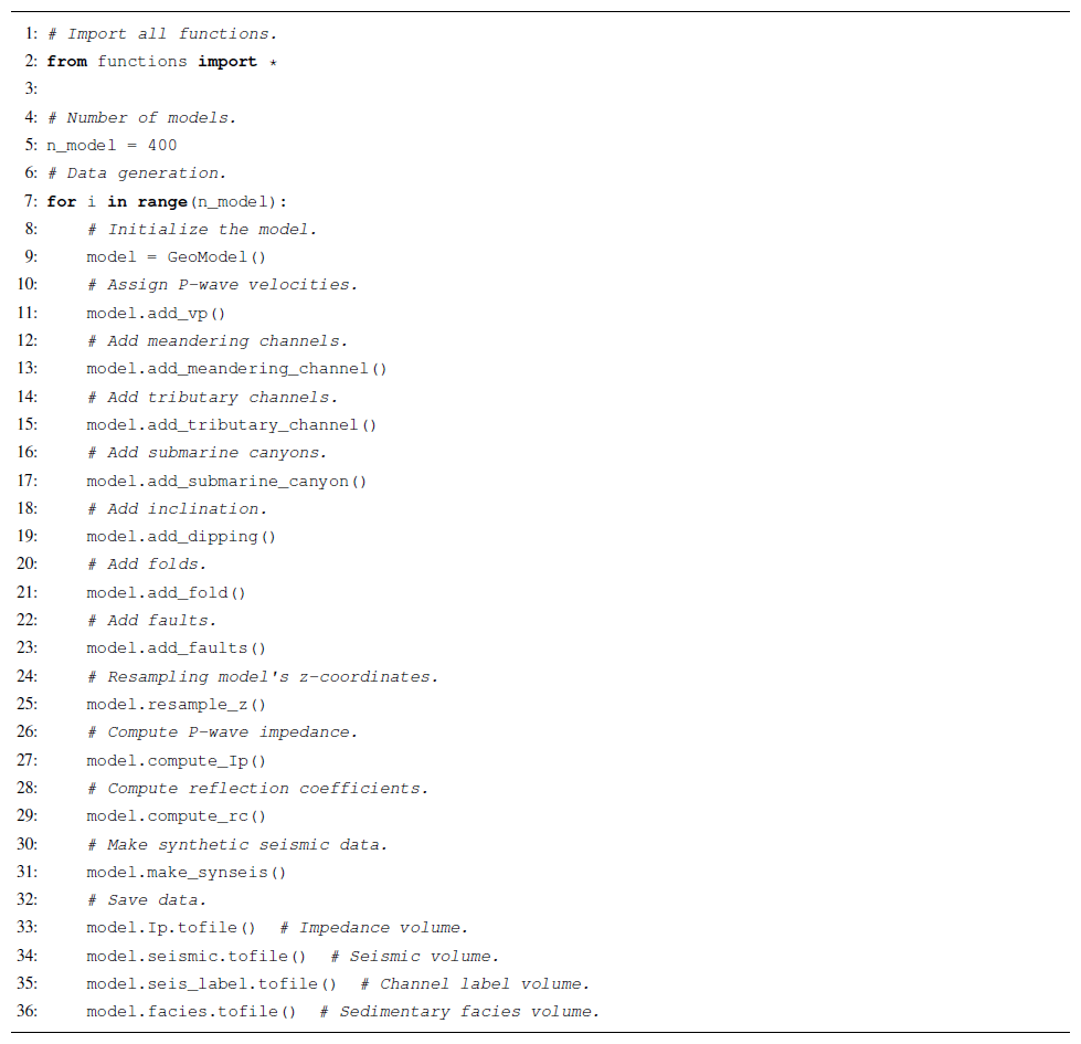
Table D1 Parameters of the seismic impedance model and Ricker wavelet, and their reference values.