the Creative Commons Attribution 4.0 License.
the Creative Commons Attribution 4.0 License.
 | 17 Jul 2025
OLIGOTREND, a global database of multi-decadal chlorophyll a and water quality time series for rivers, lakes, and estuaries
Andras Abonyi
Carles Alcaraz
Jacob Diamond
Nicholas J. K. Howden
Michael Rode
Estela Romero
Vincent Thieu
Fred Worrall
Qian Zhang
Xavier Benito
Reversed eutrophication, called oligotrophication, has been widely documented globally over the last 30 years in rivers, lakes, and estuaries. However, the absence of a comprehensive and harmonized dataset has hindered a deeper understanding of its ecological consequences. To address this data gap, we developed the OLIGOTREND database, which contains multi-decadal time series of chlorophyll a, nutrients (nitrogen and phosphorus), and related physicochemical parameters, totalling 4.3 million observations. These data originate from 1894 unique monitoring locations across estuaries (n = 238), lakes (687), and rivers (969). Most time series cover the period from 1986–2022 and comprise at least 15 years of chlorophyll a observations. Each location is associated with catchment and hydroclimatic attributes. Trend and breakpoint analyses were applied to all time series. Chlorophyll a showed temporally variable and ecosystem-specific responses to nutrient declines with an overall declining trend for 18 % of the time series, contrasting greatly with a majority of declining trends for nutrient concentrations. We harmonized the database to ensure reproducibility and ease of access and support future updates and contributions. Available at https://doi.org/10.6073/pasta/a7ad060a4dbc4e7dfcb763a794506524 (Minaudo and Benito, 2024), the OLIGOTREND database supports collaborative efforts aimed at further advancing our understanding of biogeochemical and biological mechanisms underlining oligotrophication and ecological impacts of global long-term environmental change.
- Article
(8176 KB) - Full-text XML
-
Supplement
(508 KB) - BibTeX
- EndNote


Decades of freshwater and estuarine eutrophication in the 20th century spurred coordinated national efforts to reduce aquatic nutrient loads and subsequent algal blooms (Pinay et al., 2018). The most effective actions have included improved wastewater collection and treatment, better-coordinated watershed management, and regulation of phosphorus in detergents (Conley et al., 2009; Némery and Garnier, 2016). Evidence from rivers, lakes, and estuaries already suggests that such efforts can indeed reverse eutrophication at timescales ranging from months to years and decades in a process termed oligotrophication or reoligotrophication. However, our understanding of oligotrophication is still incomplete (Anneville et al., 2019; Hoyer et al., 2002; Ibáñez and Peñuelas, 2019), and the magnitude, direction, and timing of ecological responses to water quality improvements remain to be better detected and quantified. Declines in nutrients often coincide with a transition in primary producers in terms of quantity and community composition. The most reported change in inland and estuarine ecosystems is the systematic replacement of phytoplankton by submerged macrophytes (Ibáñez and Peñuelas, 2019). However, these shifts can follow nonlinear trajectories, which is typically explained by the occurrence of alternative stable states in lakes (Scheffer and Carpenter, 2003), rivers (Verdonschot et al., 2013), and estuaries (Duarte et al., 2009; Elliott and Quintino, 2007). Additional complexities in predicting primary producer shifts arise due to nutrient legacies in the landscape that can create lags in ecosystem response (Van Meter et al., 2021; Stackpoole et al., 2019) and the presence of dams and weirs that alter the spatiotemporal variability of nutrient mobilization and transport (Zeng et al., 2023). Indeed, a wide range of contrasting trends in nutrients and primary production (as indicated by chlorophyll a, chl a) is possible (Greening and Janicki, 2006; Kronvang et al., 2005; Murphy et al., 2022), including natural causes, such as forest growth (Nilsson et al., 2024). Due to the complexity of ecosystem responses to watershed nutrient reduction, a common predictive framework remains elusive, highlighting the need for a cross-ecosystem analysis of oligotrophication trends.
Available water quality datasets, while plentiful, remain heterogeneous and often irregularly collected and reported, hindering their use in across-system studies. Moreover, oligotrophication has been primarily focused on local and regional-scale studies (e.g. Abonyi et al., 2018; Greening et al., 2014; Minaudo et al., 2021; Sabel et al., 2020) and isolated aquatic ecosystems. Thus, the spatial extent of oligotrophication trends remain poorly constrained, and we lack an understanding of the connectivity of oligotrophication responses across the watershed-to-estuary continuum. Even the best available harmonized, large-scale water quality databases commonly exclude chl a (e.g. GRQA, Virro et al., 2021), limiting their utility to evaluate oligotrophication. Likewise, some databases may cover large numbers of observations but exclude parallel measurements of chl a and nutrients, mainly phosphorus (Nilsson et al., 2024; Spaulding et al., 2024), or are temporally limited relative to oligotrophication timescales (Brehob et al., 2024). Therefore, there is a clear need for a centralized database of paired nutrient-and-primary-producer observations at oligotrophication-relevant timescales across different ecosystems.
Here we present OLIGOTREND (Minaudo and Benito, 2024), a database of 4.3 million quality assessed public and open-access observations of water quality variables and chl a from rivers, lakes and reservoirs, estuaries, and coastal bays, enabling the joint assessment of multi-decadal oligotrophication trends across spatial scales. We collected and harmonized multi-decadal time series to facilitate its structure and reuse. The database also covers geospatial data, including catchment and waterbody attributes, climate variables, and a robust trend analysis of all water quality time series. Here we highlight some of the main findings from our first analyses of the database and describe possible research directions that OLIGOTREND holds the potential to answer.
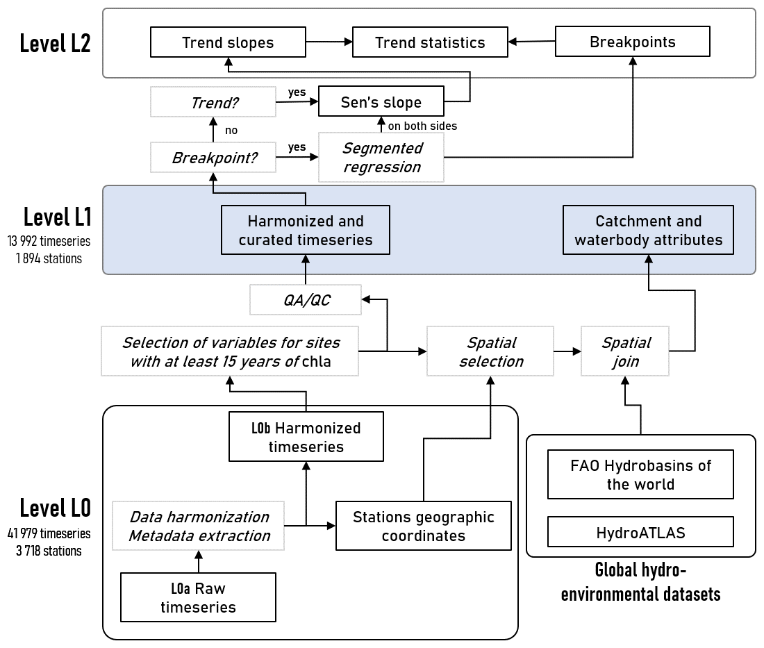
Figure 1Data levels and procedure followed to produce the OLIGOTREND database, an ensemble of harmonized and curated time series of chl a and water quality paired with catchment and waterbody attributes. QA/QC stands for quality assessment and quality check.
We followed a transparent and reproducible approach to produce the OLIGOTREND database in line with best practices for open science in ecology (Powers and Hampton, 2019). In particular, the entire data processing pipeline (Fig. 1) was developed collaboratively in a version control GitLab repository (https://gitlab.com/OLIGOTREND/wp1-unify, last access: 7 May 2025). Data are referenced according to their level (“L”) in the processing pipeline. Time series extracted from various sources were defined as “L0a”, preserving the original data structure and formatting. Time series were then harmonized (“L0b”), and a selection of variables of interest (see Sect. 2.1) at sampling sites with at least 15 years of chl a data qualified for the data quality assessment and check (QA/QC; see Sect. 2.2) and to be matched with geospatial data (see Sect. 2.3). Harmonized and curated time series together with catchment and waterbody attributes constitute “L1” data, i.e. analysis- and sharing-ready data. Any additional processing of L1 data, e.g. trend analyses, was considered “L2” (see Sect. 2.4).
2.1 Data collection
In situ chl a concentrations and physicochemical parameters were extracted from open-source international, national, and regional water quality databases (Table 1). We first obtained data from queries to the Earth System Science Data portal (https://www.earth-system-science-data.net/, last access: 17 June 2024), the Environmental Data Initiative repository (https://edirepository.org/, last access: 17 June 2024), and the Scientific Data portal (https://www-nature-com.sire.ub.edu/sdata/, last access: 17 June 2024). We then conducted a literature search on Web of Science (https://www.webofscience.com/wos/, last access: 17 June 2024) and Scopus (https://www.scopus.com/, last access: 17 June 2024) for further existing long-term chl a and nutrient time series. To do so, we used the following search terms: TITLE or ABSTRACT (oligotrophication, reoligotrophication, chlorophyll, time series); and in TITLE or ABSTRACT (lake, river, estuary, coastal, estuarine); and in EVERYTHING (trend, long term, multi-decadal). When public and accessible, we directly extracted the datasets and proceeded with data harmonization. The database architecture (Fig. 1) allows researchers to easily complement it with additional time series in the future. New additions to the database will be eased by a set of scripts available in a dedicated version control GitLab repository (https://gitlab.com/OLIGOTREND/wp1-unify, last access: 7 May 2025), allowing users to reproduce, update, or add more time series from level L0a to higher data levels and products.
We gathered data as raw measurements, i.e. unprocessed or non-aggregated time series, and defined herein these data as level L0a. Extracted variables included chlorophyll a (chl a), water temperature (wtemp), conductivity (cond), pH, dissolved oxygen as concentration (o2) and percentage of saturation (o2sat), dissolved inorganic nitrogen (din), nitrate (no3), nitrate × nitrite (no23), ammonium nitrogen (nh4), Kjeldahl nitrogen (nkjel), total nitrogen (tn), orthophosphate or soluble reactive phosphorus (po4), total phosphorus (tp), dissolved organic carbon (doc), and total suspended solids (tss). The ecosystem types covered in this database included lakes and reservoirs, rivers, estuaries, and coastal bays.
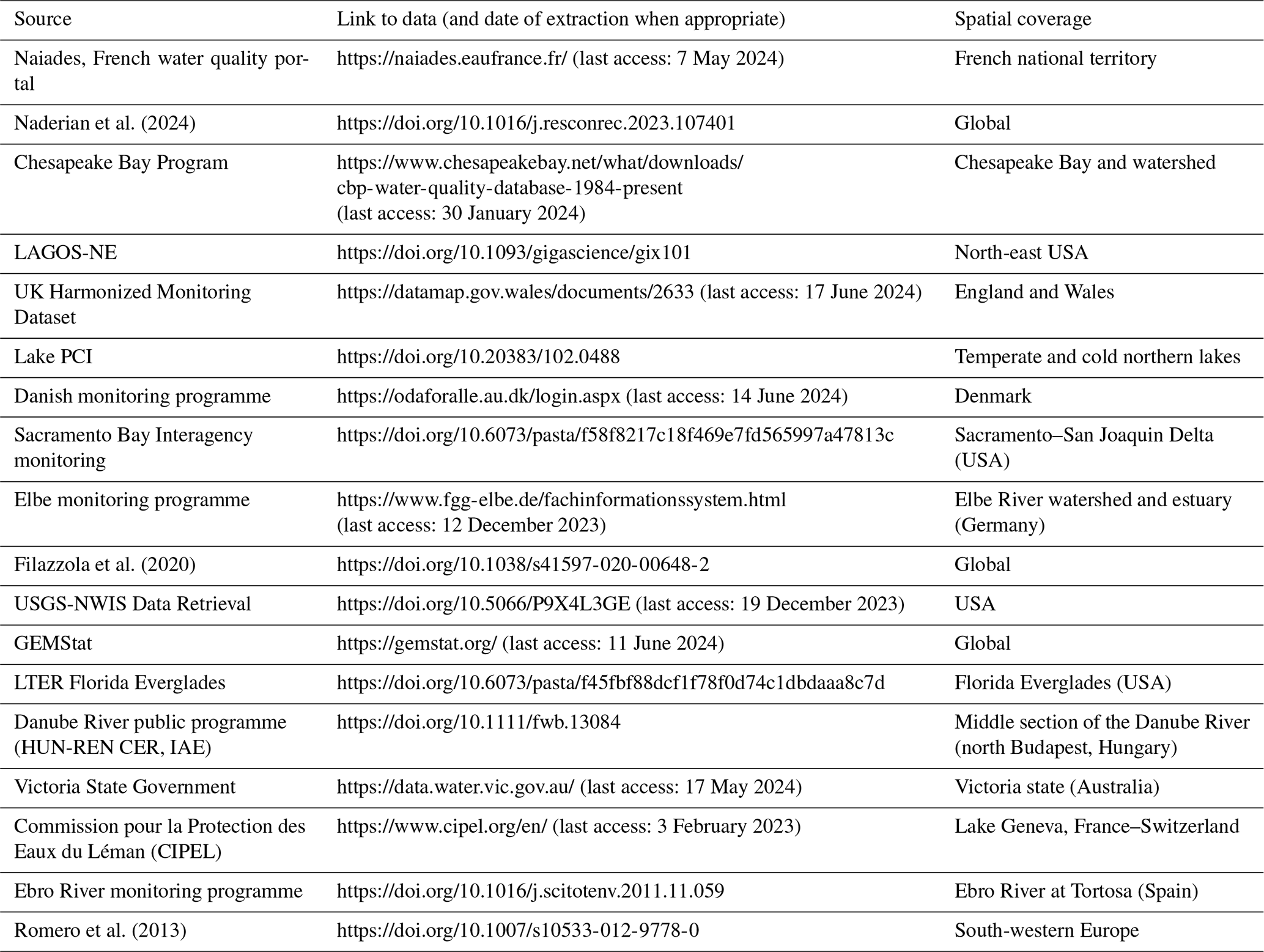
We primarily targeted databases identified with long periods of records without any filter on geographic location (Table 1). We discarded chl a datasets obtained with remote sensing techniques to ensure a strict comparability among observations. For stratifying deep lakes, we extracted values either for the euphotic layer or from the upper 10 m if euphotic depth was unavailable to avoid using data from light-limited conditions.
2.2 Data harmonization and quality control
First, L0a time series were individually reformatted into standard units and data matrix headers, forming an ensemble of time series defined here as level L0b. Nutrient concentrations were expressed as mg L−1, except chl a, which remained in µg L−1. Time series were named with a unique identifier (uniquID) per site corresponding to the concatenation of the following data separated by underscores: “ecosystem type”, “basin”, and “station ID”, e.g. “river_loire_04000100”. Basin names were derived from site geographic coordinates and the corresponding watershed according to the FAO dataset (Food and Agriculture Organization of the United Nations and FAO Land and Water Division, 2011). Ecosystem type was either “estuary”, “lake”, or “river”, corresponding to estuary or coastal bay, lake or reservoir, and river, respectively. The “station ID” was the one provided by the original data source. For each sampling site, the geographic coordinates found in the original metadata were used to create a point shapefile labelled with the station unique identifier (uniquID) as explained above. Stations with no geographic coordinates were discarded from the database.
Data quality was assessed and checked for all L0b time series from sampling stations presenting at least 15 years of chl a data. The resulting dataset comprises the OLIGOTREND L1 data level (Fig. 1). We did not remove any data in response to data curation (QA/QC) to allow users to design their own quality check procedure. Instead, we flagged potentially anomalous or suspicious observations. Valid observations were indicated with flag = 0. Quality control identified missing values (flag = 1), possible outliers (flag = 2), and abnormally repetitive values (flag = 3). Observations were considered outliers when the corresponding values exceeded 3 times the interquartile range defined by a site. Observations were considered abnormally repetitive when, at a given site and for a given variable, the corresponding value appeared more than 5 % of the time in the time series, not necessarily consecutively. Obvious mistakes in the units found in the original datasets at level L0b were identified and corrected by plotting the density of the distribution of observed concentrations and scatterplots by pairs of variables (e.g. chl a vs. tp, tp vs. po4, etc.) throughout the database.
2.3 Link with watershed and ecosystem properties
We linked inland sampling stations with the global HydroATLAS database (Lehner et al., 2022; Linke et al., 2019). The HydroATLAS has three distinct datasets: BasinATLAS, RiverATLAS, and LakeATLAS, which represent the sub-basin delineations (polygons), river network (lines), and lake shorelines (polygons), respectively. Although we proceeded with the spatial join between HydroATLAS and OLIGOTREND stations, we acknowledge there may be a potential temporal mismatch between HydroATLAS properties and OLIGOTREND temporal coverage. Yet, we assumed this spatial join would succeed at demonstrating the great variability of watershed and ecosystem properties encountered in the OLIGOTREND database.
First, we linked all OLIGOTREND sampling stations to the BasinATLAS by spatial selection of polygons of sub-basins (Pfafstetter level 12, i.e. the highest hierarchical sub-basin level in the BasinATLAS), overlapping with the point shapefile of L1 OLIGOTREND stations. A selection of watershed properties related to their physiography, climate, land cover, hydrology, and anthropogenic pressures was extracted and linked to each station present in the database at the L1 level and intersecting with one of the BasinATLAS sub-basins. Similarly, the intersection of LakeATLAS lake polygons with L1 stations provided an ensemble of lake characteristics for 61 % of the lake stations (418 out of 687). Finally, OLIGOTREND L1 river stations were linked to the RiverATLAS database by identifying the three nearest river segments using the function joinbynearest() in QGIS 3.26.2. For each possible station–segment match, the distance between the station and each segment was calculated, and the quality of the spatial join was assessed using a flagging system: if the distance to the nearest segment exceeded 500 m, a flag (flag = 1) was raised, indicating that the distance might be too large for the join to be considered valid. If the distance to the second- or third-nearest segment was less than 10 % greater than the distance to the nearest segment, a flag (flag = 2) was raised indicating that several river segments could potentially be selected. In that case, if these segments were associated with multiple sub-basins (HYBAS_L12 in HydroATLAS documentation), a flag value of 2.1 was set. If these segments were linked to multiple drainage basins (MAIN_RIV in HydroRIVERS), a flag value of 2.2 was set. All other associations identified during the spatial join were considered valid, and the flag value was set to flag = 0. Only stations with flag = 0 were considered reliable. Overall, out of 924 river stations, 90 % was considered valid. We found that 6.1 % of stations were more than 500 m away from the closest HydroRIVERS segment, and 3.9 % showed possible multiple associations (flag ≥ 2), sometimes with different sub-basins (1.3 %, flag = 2.1) or drainage basins (0.3 %, flag = 2.2). We acknowledge that there is some uncertainty in the spatial join between OLIGOTREND river stations and HydroRIVERS given the spatial resolution of the HydroSHEDS (15 arcsec). This uncertainty could be reduced using a river network derived from a higher-resolution digital elevation model. Stations with unmatched basin, lake, or river segment from the HydroATLAS database were not removed from the OLIGOTREND database, but we did not account for them in the statistics and description of watershed attributes.
2.4 Time series metrics and trend analysis
We described the OLIGOTREND time series based on multiple metrics. These included the number of observations by each variable and the extent of the period of record as well as the median, average, and standard deviation of all valid values over the entire time series.
As a first step into the trend analysis, we quantified the proportion of time series showing lower annual averages in the second half of the time series compared to the first one. We chose annual averages over growing season averages to increase robustness in the metric because sampling frequency was sometimes unequally distributed seasonally. This further simplified the question of how to identify the growing season among sites across latitudes. We considered that a lower average value in the second half of the time series indicated decline, regardless of the level of trend complexity found in the time series.
A breakpoint and segmented regression analysis was performed using the R package segmented (Fasola et al., 2018). Whenever the Davies test (Davies, 1987) did not identify any non-constant linear regressions in time series, we conducted a Mann–Kendall trend analysis on annual averages with the R package trend (Pohlert, 2023). When the Mann–Kendall test detected a monotonic trend (p < 0.01), we calculated a Sen's slope over the complete dataset. Whenever the Davies test identified non-constant linear regressions, we fitted a segmented regression to the data with two joined segments, and the position of the temporal breakpoint and the corresponding interval estimation were identified. Sen's slope was then quantified for both sides of the given breakpoint. For each segment, there were three possible trend types: declining, no trend, and rising, noted as “−”, “0”, and “+”, respectively. The combination of two joined segments or a single segment only when no breakpoint was detected provided a total of 12 possible trend types: ”−”,”−−”, ””, ”0−”, ”−0”, ”0”,”00”, ”+0”, ””,”0+”,”+”, and “”. We acknowledge a segmented regression with one breakpoint is unlikely to capture all the variety in trend patterns, but it may provide a comprehensive first assessment for nonlinear and non-monotonic temporal patterns robust enough to provide a first overview on multi-decadal temporal trajectories. Outputs from the trend analysis and above-described statistical descriptors constitute level L2 data.
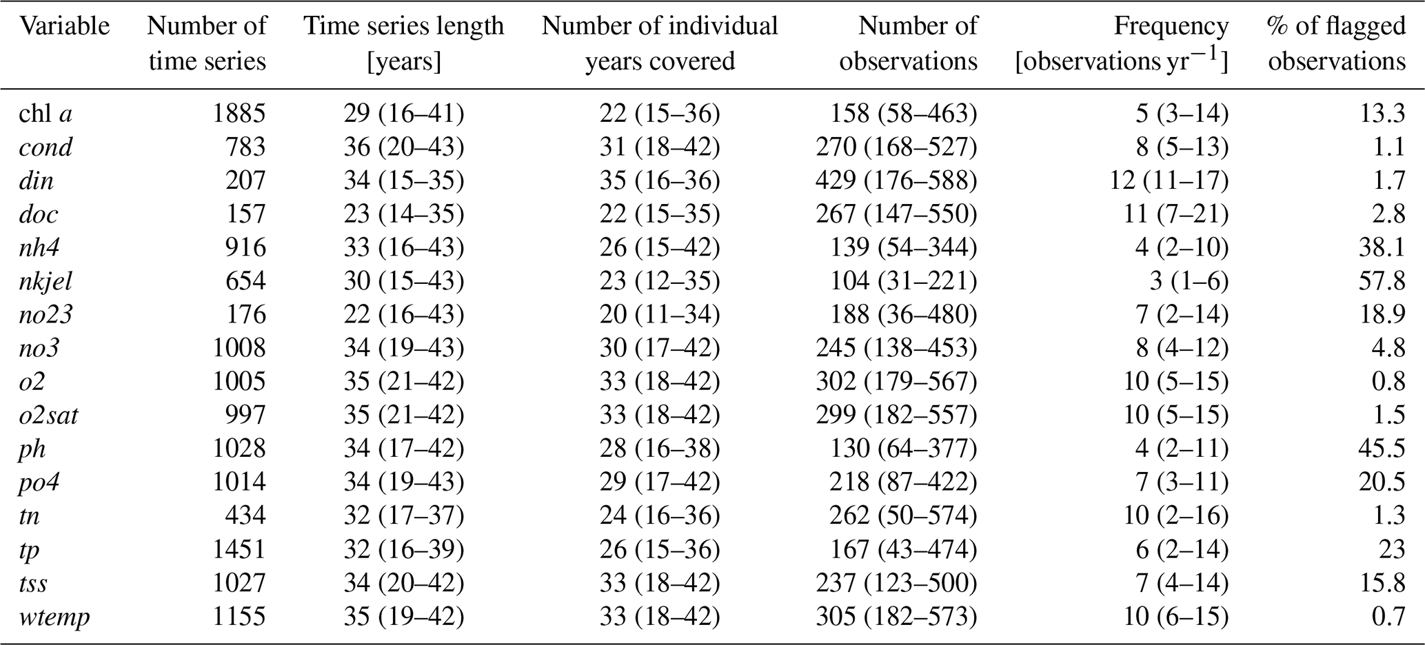
Table 2Overview of L1 data and percentage of data points flagged as invalid for each of the main variables. Ranges are presented as “median (10th percentile–90th percentile)”. The percentage of flagged observations (last column) correspond to possible outliers and abnormally repetitive values.
3.1 Time series characteristics
We collected L0 data from 3718 sampling stations, producing a total of 41 979 time series. Among these, 1894 stations had at least chl a for over 15 years and were selected for quality check and harmonization at level L1 (Fig. 1). Following the quality check, the OLIGOTREND database includes 4.3 million observations. Across all variables and time series, 83 807 observations (1.7 % of total observations) were flagged as outliers and 691 000 (13.7 % of total observations) as repetitive observations. The highest proportion of abnormally repetitive observations was found for nh4 and tp (34 % and 21 % of the observations, respectively, Table 2), likely related to detection and/or quantification limits above the actual concentrations. For chl a, 13 % of the observations was flagged as repetitive (9.9 %) or extreme outliers (3.4 %). We only included the valid data points for all subsequent analysis and time series descriptions. Most L1 time series were multi-decadal with a median time series length of 33 years (Table 2).
The majority of chl a time series included five observations per year (Table 2); only 16 % of time series were based on monthly sampling. We counted that 95 % of chl a time series exceeded 15 years and 75 %, 43 %, and 11 % covered 20, 30, and 40 years, respectively. The longest chl a time series covering more than 45 years originated from the Lake PCI dataset (10 lake chl a time series located in Sweden), the UK Harmonized Monitoring Program (42 rivers in England and Wales), and the Sacramento Bay Interagency monitoring (13 stations in estuarine area).
Time series duration and mean observation frequency for all other variables were generally similar to the chl a time series. The median period of record was 32 years for both tp and tn. Median sampling frequency was 6 and 10 observations per year for tp and tn, respectively. A small proportion (2 % and 1.8 %, respectively) of tp and tn time series were shorter than 15 years. For tp, 84 %, 57 %, and 9 % of the time series were longer than 20, 30, and 40 years, respectively. For tn, 83 %, 61 %, and 5 % of the time series were longer than 20, 30, and 40 years, respectively. There were 444 stations with joint chl a, N, and P observations for over 15 years. Among these, 220 corresponded to river stations, 169 to estuary stations, and 55 to lake stations.
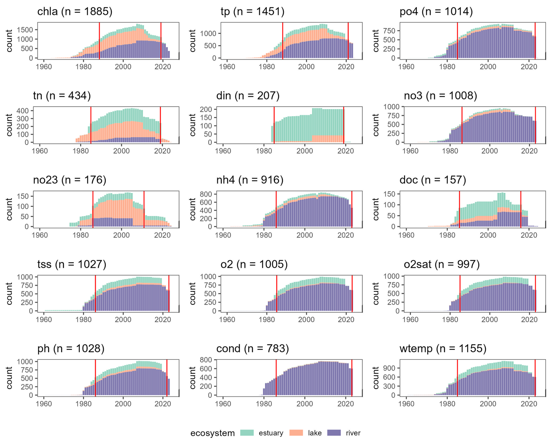
Figure 2Temporal coverage of OLIGOTREND time series for each environmental variable. The y axis “count” shows the number of time series with valid observations for each year between 1960 and 2024. Only 35 time series started before 1960; 20 concerned tss and only 1 chl a. Vertical red lines indicate median starting and ending years across the pooled dataset, i.e. the periods with the highest number of observations globally.
Table 3Characteristics of the time series constituting the OLIGOTREND database organized by data source (see Table 1). See Table S1 or similar statistics organized by basins. For the length of time series, number of observations per time series, and chl a sampling frequencies, we provide the median value, and 10th and 90th percentiles are indicated in brackets.
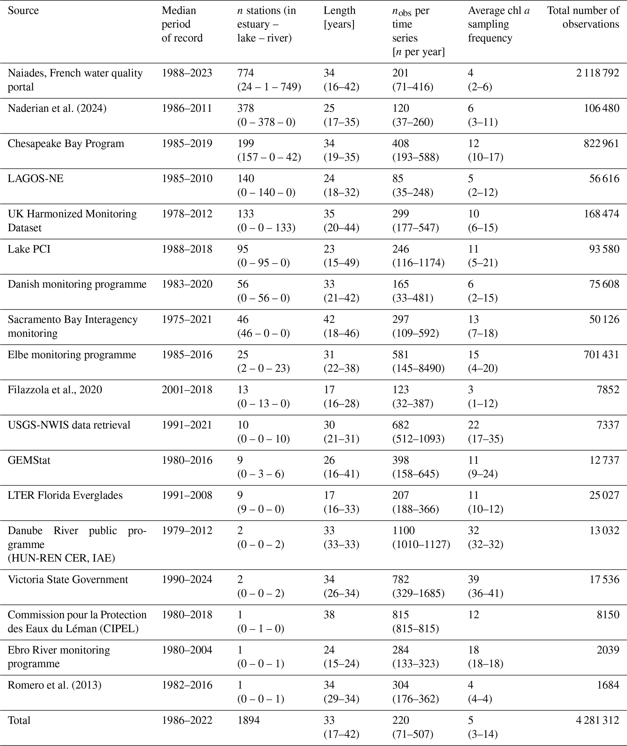
Across all time series, the median temporal coverage was 1986 to 2022 (Table 3 and Fig. 2). Yet, OLIGOTREND featured early and long chl a time series, with 19 of them starting before 1970 and an average of 50-year-long time series, most of them found in the Lake PCI dataset. Across all variables, the 2000s and 2010s are the decades with the highest coverage. The 2020s were not as covered as the 2010s were, likely indicating that databases are not systematically updated with the most recent observations.
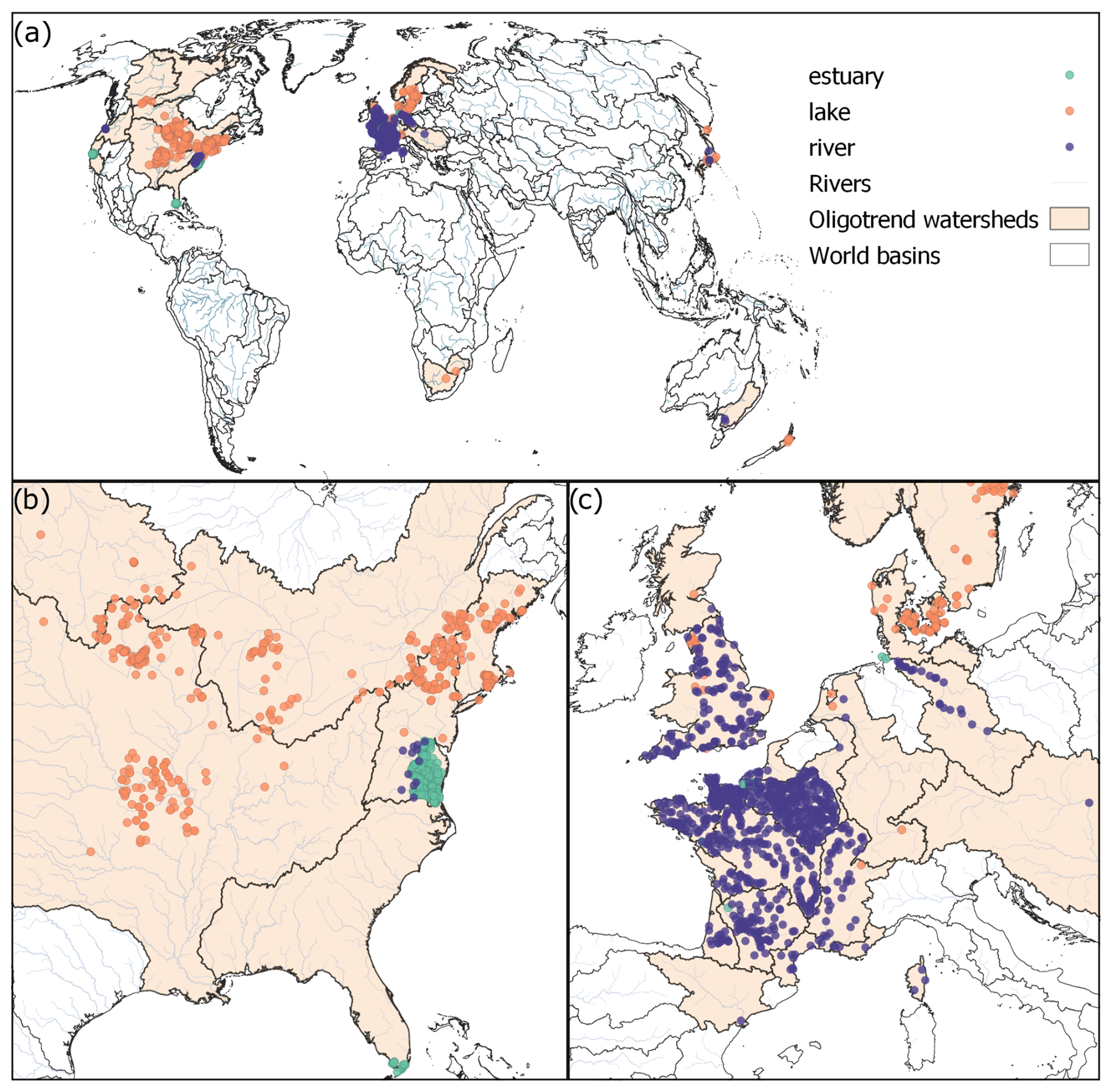
Figure 3(a) Map highlighting the 1894 sampling stations included in the OLIGOTREND database at level L1 categorized by ecosystem types. (b) Close-up on the eastern side of the US and (c) on Europe showcasing most data points from France, UK, and Denmark.
3.2 Spatial coverage
The OLIGOTREND L1 database contains 13 992 time series originating from 1894 sampling stations spanning across 5 continents (Table 1, Fig. 3). There are 238, 687, and 969 stations located in estuaries or coastal bays, lakes or reservoirs, and rivers, respectively (Table 3). The three largest data sources are the French national water quality monitoring portal (775 stations), a global database of water quality measurements in lakes (Naderian et al., 2024; 378 stations), and the United States' Chesapeake Bay Program (199 stations).
Geographically, the L1 dataset includes stations from 33 different large watersheds (Fig. 3, and see Table S1 in the Supplement for a detailed list of these watersheds). The five most represented large watersheds are the Seine (France, 320 stations), the United States North Atlantic coast (266 stations), the Mississippi–Missouri Basin (231 stations), the French west coast (183 stations), and England and Wales (163 stations). In total, 7 large watersheds contain more than 100 stations. Data from the Chesapeake Bay (United States North Atlantic coast watershed) and the Elbe River watershed are particularly remarkable in terms of data contribution, covering hundreds of stations along the main rivers and encompassing both freshwater and estuarine zones.
Table 4Basin characteristics covered by the OLIGOTREND database based on the HydroATLAS (level 12), HydroLAKES, and HydroRIVERS databases. “Range” column indicates median values, and percentiles 10 and 90 are shown in brackets.
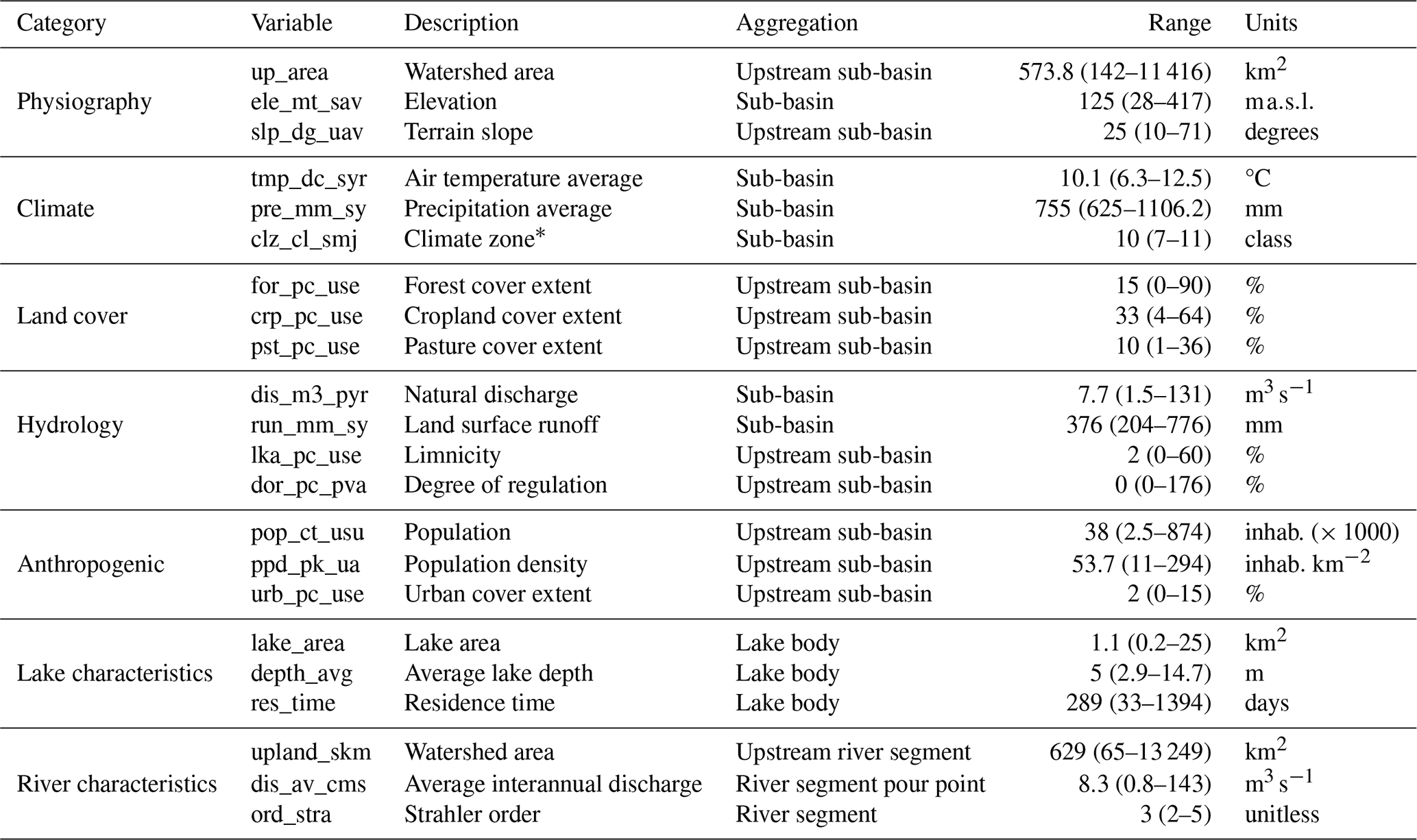
∗ Climate zone classes encompass the following classes: extremely cold and mesic, cool temperate, warm temperate, and hot and dry.
The OLIGOTREND database covers 1229 sub-basins from the HydroATLAS database, distributing over 257 spatially independent large watersheds with no hydrological connections. OLIGOTREND covers a wide range of eco-physiographic contexts (Table 4). It covers medium to large watersheds (10th to 90th percentiles were 142 to 11 416 km2), primarily lowlands. Stations extend to four climate zones, from extremely cold and mesic to hot and dry. The share among land-use types also covers a wide range, from 100 % forest or natural grassland areas to heavily impacted urban areas and croplands. Some of the stations are located in nearly pristine areas, but most of them are in highly populous areas.
Similarly, lakes and rivers represented by the OLIGOTREND database cover a wide range of morphometry, from shallow (e.g. Hickling Broad Lake, England, average water column depth ∼ 0.7 m) to deep and large lakes (e.g. Lake Geneva, France–Switzerland, average depth ∼ 155 m) and from headwater streams (e.g. the Evel River in French Brittany draining a basin of 5 km2) to large rivers (e.g. Mississippi, Danube, Rhine, Loire, Seine, Ebro, and Susquehanna rivers).
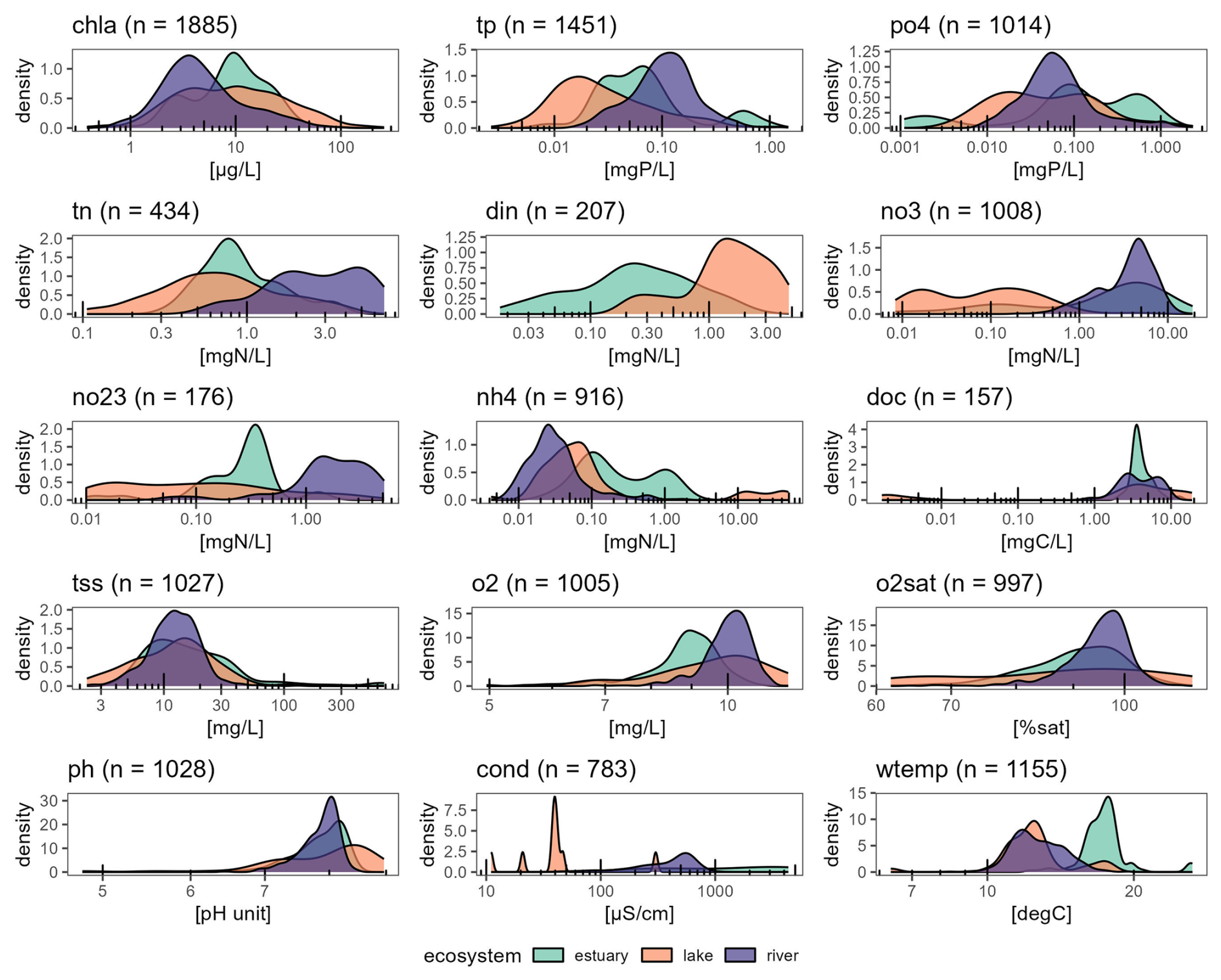
Figure 4Distribution of interannual average concentrations of all the OLIGOTREND time series. Number of time series for each variable is indicated in brackets for each variable.
3.3 OLIGOTREND time series ranges and relationships
For most variables, long-term averages are clustered by ecosystem type (Fig. 4). The lowest chl a concentrations were found in rivers (7.8 ± 10.7 µg L−1) followed by estuaries (11.8 ± 9.9 µg L−1) and then lakes (18.0 ± 25.3 µg L−1). This greatly contrasted with most P, N, and oxygen time series: for instance, tp and tn distributions showed the highest ranges in rivers (0.13 ± 0.11 mg P L−1 and 3.1 ± 1.8 mg N L−1) and the lowest in lakes (0.06 ± 0.13 mg P L−1 and 1.9 ± 0.9 mg N L−1). For DOC, most time series remained within a similar range of values regardless of ecosystem type, except for four lakes located in the north-east US (global lake database; Naderian et al., 2024). The highest conductivity values appeared in estuaries, much higher than in rivers or lakes. There were only nine lakes with conductivity time series, which explains the density distribution peaks for this ecosystem type. The warmest waters were also found in estuaries.
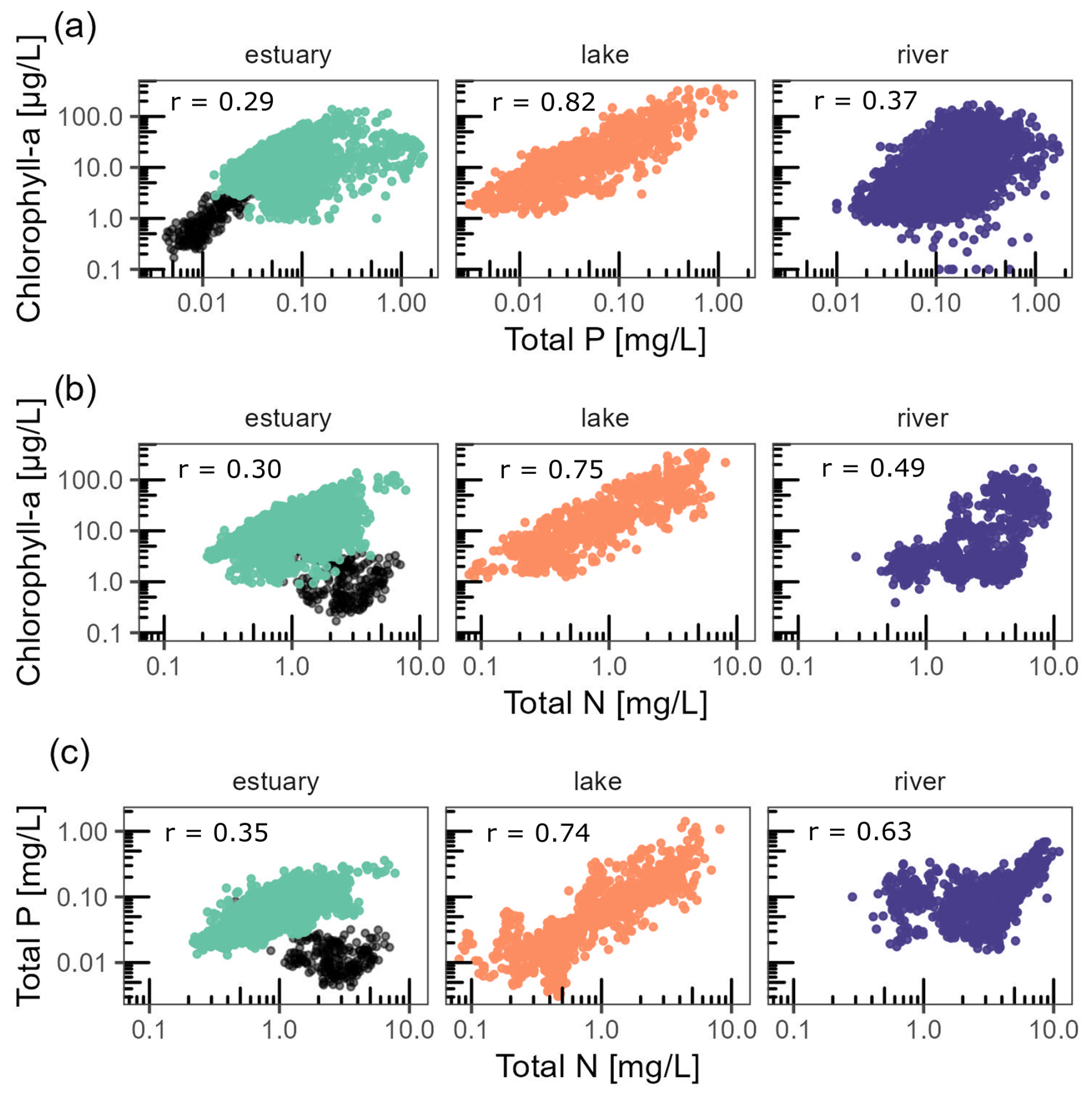
Figure 5Relationships between chl a and tp (a), chl a and tn (b), and tp and tn (c). Each dot represents the annual mean for a given time series. Dark dots for estuary stations highlight the observations in the Florida Coastal Everglades, which clearly stand out from all other estuarine observations. Pearson correlations are all statistically significant (p value < 2 × 10⁻¹⁶), and the corresponding coefficients (r) are indicated in each panel.
Across the entire database, chl a annual averages showed moderate to strong correlation with tp and tn (Fig. 5). Chl a was strongly and positively correlated with tp (Pearson, r = 0.39) across all ecosystem types. The positive correlation was the strongest for lakes (r = 0.82), moderate for rivers (r = 0.37), and the weakest for estuaries (r = 0.29). Chl a was positively correlated with tn (Pearson, r = 0.40), which was the highest in lakes (r = 0.75), moderate in rivers (r = 0.49), and the lowest in estuaries (r = 0.30). Variables tp and tn were positively correlated across all ecosystem types (Pearson, r = 0.59), with the strongest correlation found in lakes (r = 0.74), slightly lower in rivers (r = 0.63), and the weakest one in estuaries (r = 0.35). There was a clear cluster outlier for these variables in estuaries characterized by low chl a and tp but rather high tn. These observations corresponded exclusively to the Florida Coastal Everglades.
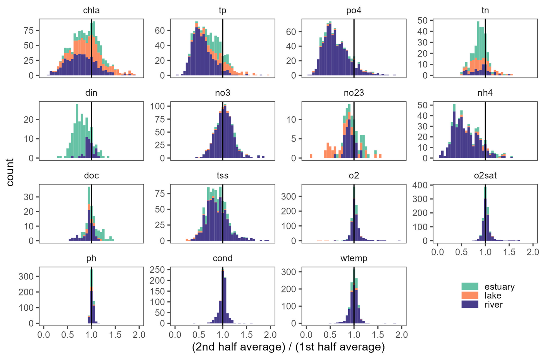
Figure 6Distribution of the ratio between second-half time series averages over first-half averages. Values significatively below 1 likely indicate declining trends regardless of the complexity of the temporal trajectory.
3.4 Trends in the OLIGOTREND database
Comparing the mean value of annual averages between the second and the first halves of time series proved to be a simple but effective way to overview temporal behaviour of time series in the database. Across all variables and ecosystem types, 60 % of time series showed a lower average value in the second half. 63 % of chl a time series showed lower values in the second half (Fig. 6). For N and P nutrient time series, 78 % to 87 % showed an average concentration that was lower in the second half (it was 85 %, 87 %, 78 %, 85 %, and 86 % for tp, po4, tn, din, and nh4, respectively). An exception was found for no3 with only 45 % time series having a lower concentration in the second half of the time series. Interestingly, we found that the majority (74 %) of tss time series had a lower concentration in the second half, whereas o2, o2sat, pH, and cond showed no clear differences in the second half of the time series with 49 %, 43 %, 42 %, and 42 %. For wtemp, there was a clear indication of a warming trend with 64 % of time series with higher averages in the second half of the time series.
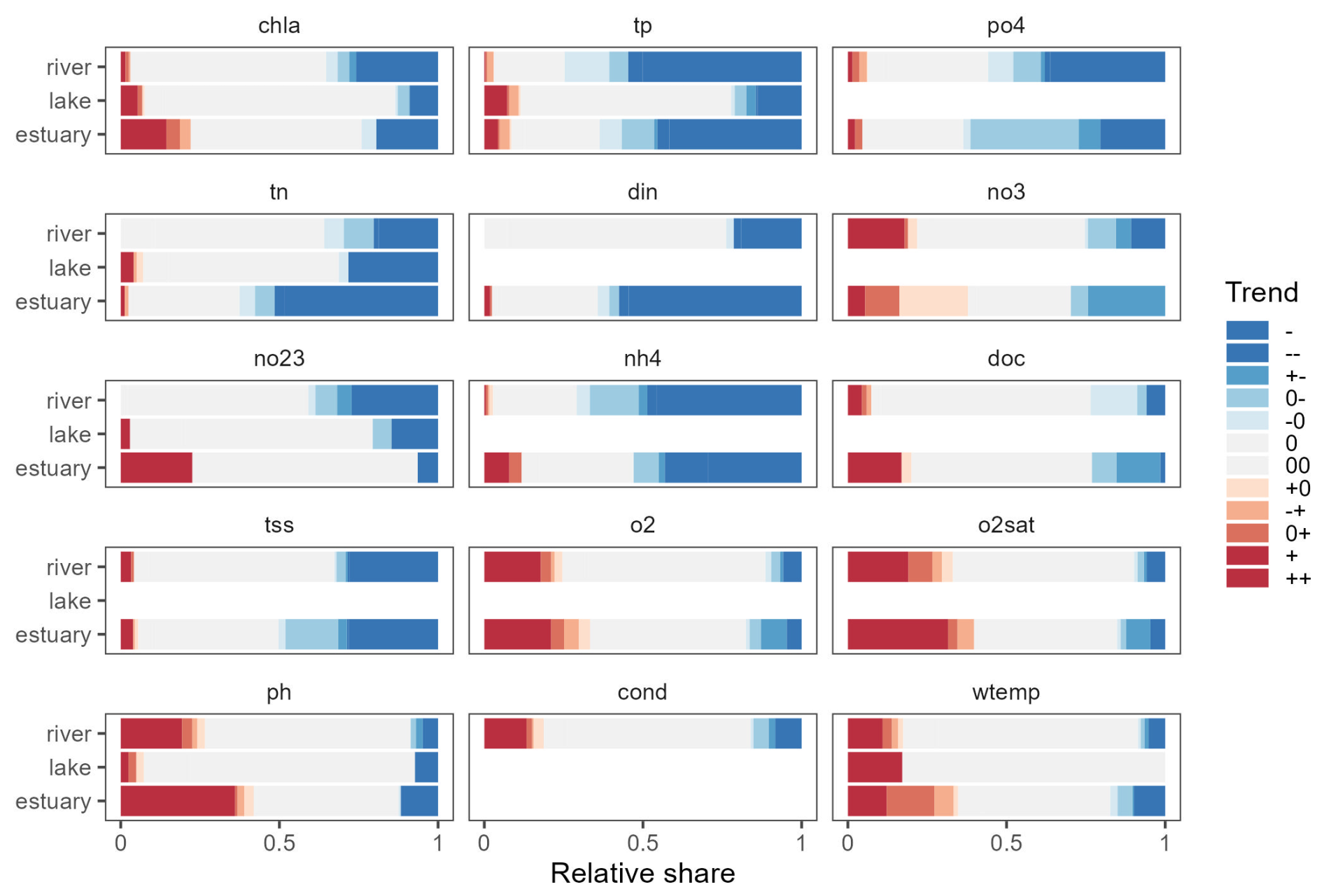
Figure 7Overview of trend significance and trend types identified in the OLIGOTREND database. Blue stripes are indicative of declining trends, grey stripes of no trend, and red stripes of rising trends. Empty stripes indicate variables or ecosystems where the number of time series available was lower than 30. Refer to Sect. 2.4 for a detailed explanation of trend symbols indicated in the legend.
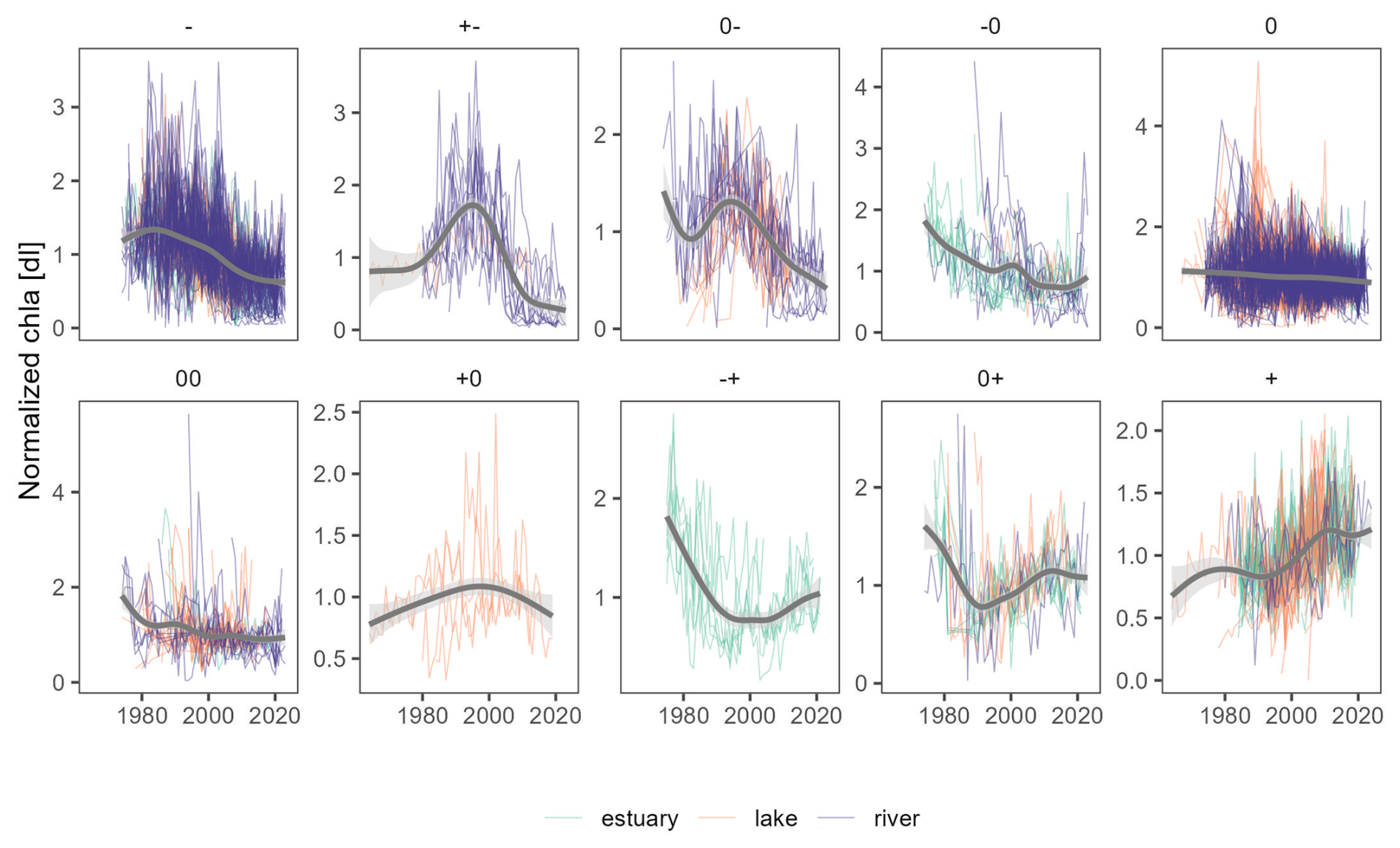
Figure 8Overview of all chl a annual time series normalized by interannual averages (thin lines), organized by trend types (panels) and ecosystem type (colour). Thick grey lines are smoothed curves of all time series within a given panel, only displayed to guide the reader. Refer to Sect. 2.4 for a detailed explanation of trend symbols indicated on top of each panel.
The breakpoint and trend analysis (Fig. 7) revealed 15 % of chl a time series were best represented with a segmented trend component, while 62 % had no trend detected, 18 % presented a monotonic declining trend, and 5 % showed a monotonic rising trend (predominantly found in estuaries; see Fig. 8). The predominant segmented trend types were “00” (32 %), “0−” (21 %), “−0” (19 %) and “” (7 %).
For tp and po4, 29 %–31 % of the time series had a breakpoint with a segmented trend, and 26 %–32 % had no trend detected, while 35 %–42 % presented a declining monotonic trend, and 1 %–2 % were rising. For tp time series, 72 % of segmented trends had a declining trend type, while it was 65 % for po4 time series. Compared to rivers and estuaries, a lower proportion of declining tp trends were observed in lake time series.
For N species, time series were dominated by the no-trend type (38 %–61 %), and significant trends were contrasted: tn, din, and nh4 showed a large number of declining trends (36 %–42 %) and a small proportion of rising trends (less than 2 %), while no3 and no23 were characterized by a larger proportion of rising trends (7 % for no23 and 17 % for no3) and segmented trends (14 % for no23 and 25 % for no3). For no3, 57 % of segmented trends had a declining trend type on the most recent part of the time series as 34 % were “0−”, and 23 % were “”. Other variables were characterized by 50 %–60 % of no-trend time series. Interestingly, among the detected trends, tss showed a significant proportion of declining trend types, while o2, o2sat, pH, and wtemp showed a predominance of rising trends.
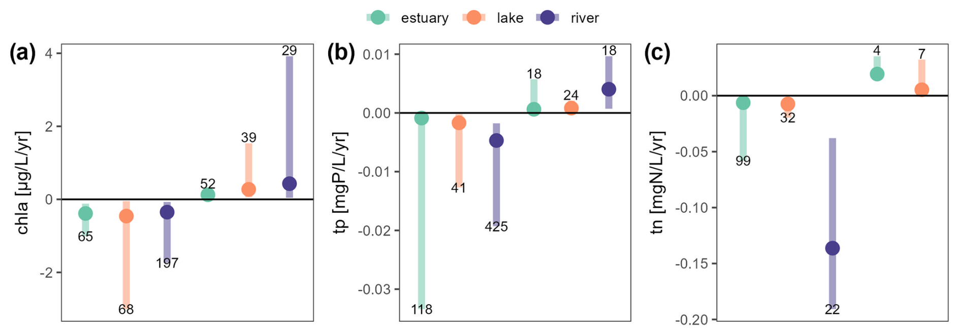
Figure 9Overview of all Sen's slopes calculated for chl a (a), tp (b) and tn (c) whether they are showing a declining (negative values) or a rising trend (positive values). Medians by ecosystem type are indicated with a plain circle, and 10th and 90th percentiles correspond to the segment ends. The numbers of time series found for each variable, ecosystem and trend type are indicated at the bottom or the top of each segment. See Fig. S1 in the Supplement for a similar figure for all variables included in OLIGOTREND.
For chl a, Sen's slopes in estuaries were smaller in magnitude compared to lakes and rivers regardless of the trend type (Fig. 9a). Lakes exhibited a median Sen's slope of −0.7 ; it was −0.4 in rivers and −0.3 in estuaries. The fastest declines (below −4 ) were found in the Sacramento Bay in California; the Loire (France); and several shallow lakes in the Mississippi–Missouri Basin, the Denmark–Germany coast, and England and Wales. The largest positive chl a trends were found in rivers, with a median slope of 0.79 compared to 0.13 and 0.23 in estuaries and lakes, respectively. The fastest rises (above 4 ) were found in the Loire (France).
For tp, the fastest rises and declines were observed in river ecosystems (Fig. 9b) with median slopes of 4.0 × 10⁻³ and −4.7 × 10⁻³ , respectively, 1 order of magnitude greater than the slopes observed in lakes and estuaries. The fastest declines (below −0.1 ) were observed in the Rhône and Seine rivers (France).
For tn, although the fastest declines were observed in estuary stations (Florida Coastal Everglades) down to −0.4 , the median value for declining slopes was overall faster in rivers with median slopes of −0.14 (Fig. 9c). It was −6 × 10⁻³ in estuaries and −7 × 10⁻³ in lakes. Only 11 stations showed rising tn trends (Fig. 7), and among them, 3 were in the Chesapeake Bay (US North Atlantic coast), which contrasted with the 145 other estuarine stations in this basin that either showed declining trends (n=89) or no trends (n=56). Note that only seven lacustrine stations showed rising tn and in rivers and that none of the tn time series showed a rising pattern.
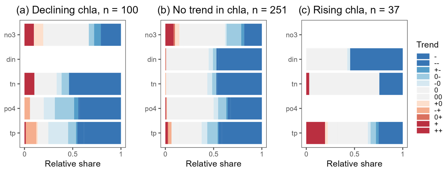
Figure 10Relative share of trend types found for nitrogen and phosphorus concentrations related to chl a time series with declining trends (a), no trends (b), and rising trends (c). This analysis is based on 444 stations having parallel measurements of chl a, and N (din and/or no3 and/or tn) and P (po4 and/or tp) for at least 15 years. Empty rows correspond to variables with less than 30 time series.
We identified 444 stations with joint chl a, P, and N data over 15 years and with more than 6 observations per year. Among these, 100 (or 23 %) chl a time series showed a linear declining trend, 251 (or 57 %) had no trend, and 37 (or 8 %) were rising. Declining chl a time series were also linked to declining trends in N and P (Fig. 10a). Nearly half of the chl a time series with no trend had corresponding no-trend or declining patterns in nutrient time series (Fig. 10b). Rising chl a time series predominantly corresponded to no-trend or declining patterns in nutrient time series. Only 18 % of the rising chl a time series also had significant rising trends in N or P.
The OLIGOTREND database has the potential to answer some important questions in large-scale aquatic ecology, biogeochemistry, and global change studies. Below, we highlight the most important findings of the database and discuss potential implications for future research beyond disciplinary boundaries.
4.1 Unravelling the ambiguous links between chl a and nutrient levels for lakes, rivers, and estuaries
The development of primary producers is far more complex than a single relationship with nutrient availability, especially if one also considers the differences among ecosystem types. Hydraulic flushing, turbulence, exposition to solar radiation, temperature (e.g. Reynolds, 2006), and light climate (Hilt et al., 2011) are crucial environmental variables in lotic systems. Water residence time, internal loading (Jeppesen et al., 2005; Krishna et al., 2021), stratification regime, and underwater light climate are other crucial factors controlling lentic ecosystems (Donis et al., 2021). Such differences are also reflected in the OLIGOTREND database. For instance, on the one hand, rivers had the highest P and N concentrations followed by estuaries and lakes, and on the other hand, the highest chl a concentrations were found in lakes followed by estuaries and then rivers (Fig. 4). Further, only 18 % of the chl a time series showed a linear declining trend, which contrasted greatly with a dominating decreasing trend for most nutrient concentrations (Figs. 6, 7, and 10). Moreover, although lake time series showed the highest correlation between chl a and nutrients (Fig. 4), they were also the ones with the highest proportion of non-significant trends (Fig. 7). In this context, we argue that the OLIGOTREND database provides a unique opportunity and foundation to further investigate the ambiguous links existing between chl a and nutrient levels over many contrasted waterbodies located in basins with different environmental and climatic conditions.
4.2 Is oligotrophication specific to aquatic ecosystem types?
The OLIGOTREND database evidenced different responses of the individual ecosystem types to nutrient declines (Figs. 7, 8, and 10). For instance, compared to estuaries and lakes, rivers showed the highest proportion of declining chl a (Fig. 7). The inherent specificities of different ecosystems could partly explain why oligotrophication seems to be ecosystem-specific: (i) the successful P reduction in many rivers worldwide (e.g. Le Moal et al., 2019) has led to more frequent P limitation for phytoplankton (Elser et al., 2007), although N or Si may also be limiting primary production (Paerl et al., 2016). (ii) In lakes, longer water residence time and internal nutrient loading can either delay (Jeppesen et al., 2005) or amplify (i.e. through algal blooms; e.g. Krishna et al., 2021) the ecological response following nutrient declines. (iii) Temporal shifts in phytoplankton assemblages towards taxa better adapted to low P levels, and taxa that are barely controlled by zooplankton grazing (e.g. filamentous cyanobacteria; Selmeczy et al., 2019) can often represent overlooked effects, explaining rising or weak trends in primary producers despite nutrient decline over time (Anneville et al., 2019). (iv) In estuaries, the dynamic of primary producers is also largely affected by marine waters, where coastal phytoplankton, sensitive to N (Elser et al., 2007), or N and P availability meets freshwater phytoplankton that is primarily sensitive to P (Kemp et al., 2005). Future analysis of OLIGOTREND time series together with catchment and waterbody attributes could improve our understanding of how aquatic ecosystems respond to nutrient trends in a wide variety of aquatic ecosystems.
4.3 Abrupt and gradual changes in long-term water quality time series
The OLIGOTREND database could be explored to further evidence the extent of gradual changes or abrupt regime shifts in water quality time series. In fact, some of the waterbodies represented in OLIGOTREND are known for shifting their primary producer's structure and function following oligotrophication. This is the case of the Loire (France) and the Ebro rivers (Spain), which are known for their long-term gradual regime shifts from phytoplankton to macrophytes in response to phosphorus decline (Diamond et al., 2021; Ibáñez et al., 2012; Minaudo et al., 2015, 2021). Similarly, phytoplankton of the middle Danube now more frequently contains benthic taxa, predominantly diatoms, potentially indicating a long-term regime shift from pelagic to benthic production in recent decades (Abonyi et al., 2018). Moreover, oligotrophication can result in a shift from heterotrophic conditions to dominantly autotrophic processes with lower pollution, as observed for the Elbe River (Wachholz et al., 2024). OLIGOTREND time series could be further analysed to detect possible temporal changes in variance (as a possible early-warning signal; Dakos et al., 2015), seasonal patterns, and relationships between chl a, nutrients, and ecosystem metabolism. This could enhance our understanding of crucial factors underlying regime shifts in river ecosystems, which are comparatively less well known than in lakes (Gilarranz et al., 2022).
In OLIGOTREND, we highlighted a significant number of no-trend or rising chl a time series despite declining nutrient levels (Fig. 10c). This could be related to climatic effects and long-term changes in ecosystem structure, such as in the Chesapeake Bay (Harding et al., 2019). Future analysis of the OLIGOTREND will provide an invaluable source of data to disentangle the effects of climate change and watershed biogeochemistry on multi-decadal chl a and nutrient trends.
4.4 Combining OLIGOTREND with large-scale datasets to foster interdisciplinary aquatic data science
The OLIGOTREND database can help boost water quality research if it is combined with other large-scale or long-term ecological datasets. For instance, it is known that shifting baselines because of temporal changes in different, covarying environmental factors can preclude the return of the primary producer to pre-eutrophication conditions (Carstensen et al., 2011; Duarte et al., 2009). As global change intensifies, leading to novel ecosystems (Hobbs et al., 2009), the temporal extension of most available water quality datasets limits a correct estimation of pre-eutrophication baselines. Only a fraction of the OLIGOTREND database covers chl a and/or nutrients during the eutrophication phase, which renders pre-oligotrophication reference conditions impossible to discern and, hence, makes it difficult to validate nutrient remediation actions (Pinay et al., 2018). In this context, combining palaeolimnological observations with water quality monitoring data could have a potential not fully implemented at large spatial scales and across different aquatic ecosystem types (Bennion et al., 2015; Bhattacharya et al., 2022; Dong et al., 2012).
Recent research has shown that nutrient concentrations link to nutrient loads (point and nonpoint sources) at the catchment scale (Ehrhardt et al., 2021; Jarvie et al., 2012; Murphy et al., 2022). Yet, only a few studies have established a mechanistic link between nutrient input management and the development of the phytoplankton biomass. Data-based approaches that jointly analyse decreasing nutrient loadings over multiple decades and sites with corresponding measurements of chl a and nutrients can help better characterize how successful catchment management and environmental measures can affect reverse eutrophication. OLIGOTREND holds the potential to approach oligotrophication longitudinally at the basin scale, where long-term trajectories can be assessed from small streams, rivers, and lakes/reservoirs towards estuaries/coastal ecosystems along with their hydrologically connected time series.
Remote sensing could further supplement crucial water quality information organized in OLIGOTREND. Remote sensing can provide time series data on water quality for inland and coastal aquatic ecosystems, which, if combined with in situ measurements, can increase chl a data coverage both spatially and temporally (Ross et al., 2019; Spaulding et al., 2024). Moreover, regional and Earth system numerical models will improve further if calibrated or validated by in situ observations (Casquin et al., 2024; Liu et al., 2024). The OLIGOTREND database readily represents a centralized and harmonized dataset open for calibration and validation by remotely-sensed water quality data that is available for training and validating regional and large-scale numerical models.
Finally, there is a growing interest in large-scale observations that integrate new and existing databases to answer key questions in aquatic ecology (Barquín et al., 2015). Long-term observations of community data (e.g. via LTER and eLTER, GBIF, Biofresh) may include key functional groups of aquatic food webs, such as phytoplankton, zooplankton, macroinvertebrates (Welti et al., 2024), and fish (Comte et al., 2021). For a selection of sites, chl a trends can be further analysed jointly with long-term community data to investigate the role that community composition and biodiversity may play in responding to long-term environmental change (Jochimsen et al., 2013). Some of the OLIGOTREND time series are linked to lotic community data (i.e. phytoplankton), which have been seldom explored compared to lakes when testing the biodiversity effect on ecosystem functioning and services (Filstrup et al., 2019; Ptacnik et al., 2008).
All the data are openly available along with the R scripts used for data processing from raw measurements at the L0a level to higher data processing levels. All R scripts produced to extract, harmonize, and process the OLIGOTREND data were stored and organized in a dedicated GitLab repository (https://gitlab.com/OLIGOTREND/wp1-unify, Minaudo and Benito, 2025). Data at levels L1 and L2 (Fig. 1) were deposited in an Environmental Data Initiative Data Package accessible on the EDI data portal (https://doi.org/10.6073/pasta/a7ad060a4dbc4e7dfcb763a794506524, Minaudo and Benito, 2024). Original links to data sources of L0a data are provided in Table 1 and in the EDI data package. Additionally, we also provide in the GitLab repository all the GIS files emerging from the data extraction step, including shapefiles of L0 and L1 stations and the corresponding basin, lake, and river characteristics resulting from the spatial join between OLIGOTREND stations and the HydroATLAS.
The OLIGOTREND database provides invaluable information in aquatic ecology and Earth system science. We evidenced oligotrophication at large temporal and spatial scales and unveiled the complexity of the chlorophyll a response following oligotrophication and the relationships between chlorophyll a and nutrients in inland and transitional waters, covering a wide range of climatic and environmental conditions. While the database is not exhaustive, its flexible structure and reproducible processing pipeline facilitate the inclusion of additional datasets in the future. We also see a strong need to continuously update the database due to the accelerating climate change and the resulting impacts on the loading and processing of nutrients and the associated ecological implications (van Vliet et al., 2023). Finally, OLIGOTREND will support collaborative efforts aimed at advancing our understanding of the complex biogeochemical and biological mechanisms driving oligotrophication and the broader ecological impacts of global environmental change.
The supplement related to this article is available online at https://doi.org/10.5194/essd-17-3411-2025-supplement.
CM and XB both secured the funding for this study and contributed equally for the conceptualization, methodology, data curation, formal analysis, and investigation. They wrote the original draft together. All other authors provided datasets and participated in the revisions of the original draft.
The contact author has declared that none of the authors has any competing interests.
Publisher's note: Copernicus Publications remains neutral with regard to jurisdictional claims made in the text, published maps, institutional affiliations, or any other geographical representation in this paper. While Copernicus Publications makes every effort to include appropriate place names, the final responsibility lies with the authors.
The authors would like to thank the two anonymous reviewers whose comments and suggestions helped to improve and clarify this manuscript.
This study was funded by the Iberian Association of Ecology (SIBECOL) through the 2022 early-career advanced grant to Camille Minaudo and Xavier Benito. Both Camille Minaudo and Xavier Benito have received funding from the postdoctoral fellowships programme Beatriu de Pinós funded by the Secretary of Universities and Research (Government of Catalonia) and by the Horizon 2020 programme of research and innovation of the European Union under the Marie Skłodowska-Curie grant agreement no. 801370. Andras Abonyi was supported by the National Research, Development and Innovation Office, Hungary (project FK 142485), and by the János Bolyai Research Scholarship of the Hungarian Academy of Sciences. Estela Romero acknowledges the support of the Grant “Severo Ochoa Centres of Excellence” (CEX2018-000828-S) funded by grant no. MCIN/AEI/10.13039/50110001103 and the project KALORET (PID2021-128778OA-I00) funded by grant no. MCIN/AEI/10.13039/501100011033 and by “ERDF A way of making Europe”.
This paper was edited by Zihao Bian and reviewed by two anonymous referees.
Abonyi, A., Ács, É., Hidas, A., Grigorszky, I., Várbíró, G., Borics, G., and Kiss, K. T.: Functional diversity of phytoplankton highlights long-term gradual regime shift in the middle section of the Danube River due to global warming, human impacts and oligotrophication, Freshwater Biol., 63, 456–472, https://doi.org/10.1111/fwb.13084, 2018.
Anneville, O., Chang, C., Dur, G., Souissi, S., Rimet, F., and Hsieh, C.: The paradox of re-oligotrophication: the role of bottom–up versus top–down controls on the phytoplankton community, Oikos, 128, 1666–1677, https://doi.org/10.1111/oik.06399, 2019.
Barquín, J., Benda, L. E., Villa, F., Brown, L. E., Bonada, N., Vieites, D. R., Battin, T. J., Olden, J. D., Hughes, S. J., Gray, C., and Woodward, G.: Coupling virtual watersheds with ecosystem services assessment: a 21st century platform to support river research and management, WIREs Water, 2, 609–621, https://doi.org/10.1002/WAT2.1106, 2015.
Bennion, H., Simpson, G. L., and Goldsmith, B. J.: Assessing degradation and recovery pathways in lakes impacted by eutrophication using the sediment record, Front. Ecol. Evol., 3, 148732, https://doi.org/10.3389/FEVO.2015.00094, 2015.
Bhattacharya, R., Lin, S. G. M., and Basu, N. B.: Windows into the past: lake sediment phosphorus trajectories act as integrated archives of watershed disturbance legacies over centennial scales, Environ. Res. Lett., 17, 34005, https://doi.org/10.1088/1748-9326/ac4cf3, 2022.
Brehob, M. M., Pennino, M. J., Handler, A. M., Compton, J. E., Lee, S. S., and Sabo, R. D.: Estimates of Lake Nitrogen, Phosphorus, and Chlorophyll-a Concentrations to Characterize Harmful Algal Bloom Risk Across the United States, Earths Future, 12, e2024EF004493, https://doi.org/10.1029/2024EF004493, 2024.
Carstensen, J., Sánchez-Camacho, M., Duarte, C. M., Krause-Jensen, D., and Marbà, N.: Connecting the Dots: Responses of Coastal Ecosystems to Changing Nutrient Concentrations, Environ. Sci. Technol., 45, 9122, https://doi.org/10.1021/es202351y, 2011.
Casquin, A., Silvestre, M., and Thieu, V.: nuts-STeauRY dataset: hydrochemical and catchment characteristics dataset for large sample studies of Carbon, Nitrogen, Phosphorus and Silicon in french watercourses, Zenodo [data set], https://doi.org/10.5281/ZENODO.10830852, 2024.
Comte, L., Carvajal-Quintero, J., Tedesco, P. A., Giam, X., Brose, U., Erős, T., Filipe, A. F., Fortin, M., Irving, K., Jacquet, C., Larsen, S., Sharma, S., Ruhi, A., Becker, F. G., Casatti, L., Castaldelli, G., Dala-Corte, R. B., Davenport, S. R., Franssen, N. R., García-Berthou, E., Gavioli, A., Gido, K. B., Jimenez-Segura, L., Leitão, R. P., McLarney, B., Meador, J., Milardi, M., Moffatt, D. B., Occhi, T. V. T., Pompeu, P. S., Propst, D. L., Pyron, M., Salvador, G. N., Stefferud, J. A., Sutela, T., Taylor, C., Terui, A., Urabe, H., Vehanen, T., Vitule, J. R. S., Zeni, J. O., and Olden, J. D.: RivFishTIME: A global database of fish time-series to study global change ecology in riverine systems, Global Ecol. Biogeogr., 30, 38–50, https://doi.org/10.1111/geb.13210, 2021.
Conley, D. J., Paerl, H. W., Howarth, R. W., Boesch, D. F., Seitzinger, S. P., Havens, K. E., Lancelot, C., and Likens, G. E.: Controlling Eutrophication: Nitrogen and Phosphorus, Science (1979), 323, 1014–1015, https://doi.org/10.1126/science.1167755, 2009.
Dakos, V., Carpenter, S. R., van Nes, E. H., and Scheffer, M.: Resilience indicators: prospects and limitations for early warnings of regime shifts, Philos. T. R. Soc. B, 370, 1–10, https://doi.org/10.1098/RSTB.2013.0263, 2015.
Davies, R. B.: Hypothesis testing when a nuisance parameter is present only under the alternative, Biometrika, 74, 33–43, https://doi.org/10.1093/biomet/74.1.33, 1987.
Diamond, J. S., Moatar, F., Cohen, M. J., Poirel, A., Martinet, C., Maire, A., and Pinay, G.: Metabolic regime shifts and ecosystem state changes are decoupled in a large river, Limnol. Oceanogr., 67, S54–S70, https://doi.org/10.1002/lno.11789, 2021.
Dong, X., Bennion, H., Maberly, S. C., Sayer, C. D., Simpson, G. L., and Battarbee, R. W.: Nutrients exert a stronger control than climate on recent diatom communities in Esthwaite Water: evidence from monitoring and palaeolimnological records, Freshwater Biol., 57, 2044–2056, https://doi.org/10.1111/J.1365-2427.2011.02670.X, 2012.
Donis, D., Mantzouki, E., McGinnis, D. F., Vachon, D., Gallego, I., Grossart, H., Senerpont Domis, L. N., Teurlincx, S., Seelen, L., Lürling, M., Verstijnen, Y., Maliaka, V., Fonvielle, J., Visser, P. M., Verspagen, J., Herk, M., Antoniou, M. G., Tsiarta, N., McCarthy, V., Perello, V. C., Machado-Vieira, D., Oliveira, A. G., Maronić, D. Š., Stević, F., Pfeiffer, T. Ž., Vucelić, I. B., Žutinić, P., Udovič, M. G., Plenković-Moraj, A., Bláha, L., Geriš, R., Fránková, M., Christoffersen, K. S., Warming, T. P., Feldmann, T., Laas, A., Panksep, K., Tuvikene, L., Kangro, K., Koreivienė, J., Karosienė, J., Kasperovičienė, J., Savadova-Ratkus, K., Vitonytė, I., Häggqvist, K., Salmi, P., Arvola, L., Rothhaupt, K., Avagianos, C., Kaloudis, T., Gkelis, S., Panou, M., Triantis, T., Zervou, S., Hiskia, A., Obertegger, U., Boscaini, A., Flaim, G., Salmaso, N., Cerasino, L., Haande, S., Skjelbred, B., Grabowska, M., Karpowicz, M., Chmura, D., Nawrocka, L., Kobos, J., Mazur-Marzec, H., Alcaraz-Párraga, P., Wilk-Woźniak, E., Krztoń, W., Walusiak, E., Gagala-Borowska, I., Mankiewicz-Boczek, J., Toporowska, M., Pawlik-Skowronska, B., Niedźwiecki, M., Pęczuła, W., Napiórkowska-Krzebietke, A., Dunalska, J., Sieńska, J., Szymański, D., Kruk, M., Budzyńska, A., Goldyn, R., Kozak, A., Rosińska, J., Szeląg-Wasielewska, E., Domek, P., Jakubowska-Krepska, N., Kwasizur, K., Messyasz, B., Pełechata, A., Pełechaty, M., Kokocinski, M., Madrecka-Witkowska, B., Kostrzewska-Szlakowska, I., Frąk, M., Bańkowska-Sobczak, A., et al.: Stratification strength and light climate explain variation in chlorophyll a at the continental scale in a European multilake survey in a heatwave summer, Limnol. Oceanogr., 66, 4314–4333, https://doi.org/10.1002/lno.11963, 2021.
Duarte, C. M., Conley, D. J., Carstensen, J., and Sánchez-Camacho, M.: Return to Neverland: Shifting Baselines Affect Eutrophication Restoration Targets, Estuar. Coast., 32, 29–36, https://doi.org/10.1007/s12237-008-9111-2, 2009.
Ehrhardt, S., Ebeling, P., Dupas, R., Kumar, R., Fleckenstein, J. H., and Musolff, A.: Nitrate Transport and Retention in Western European Catchments Are Shaped by Hydroclimate and Subsurface Properties, Water Resour. Res., 57, e2020WR029469, https://doi.org/10.1029/2020WR029469, 2021.
Elliott, M. and Quintino, V.: The Estuarine Quality Paradox, Environmental Homeostasis and the difficulty of detecting anthropogenic stress in naturally stressed areas, Mar. Pollut. Bull., 54, 640–645, https://doi.org/10.1016/J.MARPOLBUL.2007.02.003, 2007.
Elser, J. J., Bracken, M. E. S., Cleland, E. E., Gruner, D. S., Harpole, W. S., Hillebrand, H., Ngai, J. T., Seabloom, E. W., Shurin, J. B., and Smith, J. E.: Global analysis of nitrogen and phosphorus limitation of primary producers in freshwater, marine and terrestrial ecosystems, Ecol. Lett., 10, 1135–1142, https://doi.org/10.1111/j.1461-0248.2007.01113.x, 2007.
Fasola, S., Muggeo, V. M. R., and Küchenhoff, H.: A heuristic, iterative algorithm for change-point detection in abrupt change models, Comput. Stat., 33, 997–1015, https://doi.org/10.1007/S00180-017-0740-4, 2018.
Filazzola, A., Mahdiyan, O., Shuvo, A., Ewins, C., Moslenko, L., Sadid, T., Blagrave, K., Imrit, M. A., Gray, D. K., Quinlan, R., O'Reilly, C. M., and Sharma, S.: A database of chlorophyll and water chemistry in freshwater lakes, Sci. Data, 7, 310, https://doi.org/10.1038/s41597-020-00648-2, 2020.
Filstrup, C. T., King, K. B. S., and McCullough, I. M.: Evenness effects mask richness effects on ecosystem functioning at macro-scales in lakes, Ecol. Lett., 22, 2120–2129, https://doi.org/10.1111/ele.13407, 2019.
Food and Agriculture Organization of the United Nations and FAO Land and Water Division: Major hydrological basins of the world, AQUASTAT (FAO) [data set], https://data.apps.fao.org/catalog//iso/7707086d-af3c-41cc-8aa5-323d8609b2d1 (last access: 28 January 2025), 2011.
Gilarranz, L. J., Narwani, A., Odermatt, D., Siber, R., and Dakos, V.: Regime shifts, trends, and variability of lake productivity at a global scale, P. Natl. Acad. Sci. USA, 119, e2116413119, https://doi.org/10.1073/pnas.2116413119, 2022.
Greening, H. and Janicki, A.: Toward reversal of eutrophic conditions in a subtropical estuary: Water quality and seagrass response to nitrogen loading reductions in Tampa Bay, Florida, USA, Environ. Manage., 38, 163–178, https://doi.org/10.1007/S00267-005-0079-4, 2006.
Greening, H., Janicki, A., Sherwood, E. T., Pribble, R., and Johansson, J. O. R.: Ecosystem responses to long-term nutrient management in an urban estuary: Tampa Bay, Florida, USA, Estuar. Coast. Shelf S., 151, A1–A16, https://doi.org/10.1016/J.ECSS.2014.10.003, 2014.
Harding, L. W., Mallonee, M. E., Perry, E. S., Miller, W. D., Adolf, J. E., Gallegos, C. L., and Paerl, H. W.: Long-term trends, current status, and transitions of water quality in Chesapeake Bay, Sci. Rep.-UK, 9, 6709, https://doi.org/10.1038/s41598-019-43036-6, 2019.
Hilt, S., Köhler, J., Kozerski, H.-P., van Nes, E. H., and Scheffer, M.: Abrupt regime shifts in space and time along rivers and connected lake systems, Oikos, 120, 766–775, https://doi.org/10.1111/j.1600-0706.2010.18553.x, 2011.
Hobbs, R. J., Higgs, E., and Harris, J. A.: Novel ecosystems: implications for conservation and restoration, Trends Ecol. Evol., 24, 599–605, https://doi.org/10.1016/j.tree.2009.05.012, 2009.
Hoyer, M. V, Frazer, T. K., Notestein, S. K., and Canfield Jr., D. E.: Nutrient, chlorophyll, and water clarity relationships in Florida's nearshore coastal waters with comparisons to freshwater lakes, Can. J. Fish. Aquat. Sci., 59, 1024–1031, https://doi.org/10.1139/f02-077, 2002.
Ibáñez, C. and Peñuelas, J.: Changing nutrients, changing rivers, Science, 365, 637–638, https://doi.org/10.1126/science.aay2723, 2019.
Ibáñez, C., Alcaraz, C., Caiola, N., Rovira, A., Trobajo, R., Alonso, M., Duran, C., Jiménez, P. J., Munné, A., and Prat, N.: Regime shift from phytoplankton to macrophyte dominance in a large river: Top-down versus bottom-up effects, Sci. Total Environ., 416, 314–322, https://doi.org/10.1016/j.scitotenv.2011.11.059, 2012.
Jarvie, H. P., Sharpley, A. N., Scott, J. T., Haggard, B. E., Bowes, M. J., and Massey, L. B.: Within-River Phosphorus Retention: Accounting for a Missing Piece in the Watershed Phosphorus Puzzle, Environ. Sci. Technol., 46, 13284–13292, https://doi.org/10.1021/es303562y, 2012.
Jeppesen, E., Søndergaard, M., Jensen, J. P., Havens, K. E., Anneville, O., Carvalho, L., Coveney, M. F., Deneke, R., Dokulil, M. T., Foy, B., Gerdeaux, D., Hampton, S. E., Hilt, S., Kangur, K., Köhler, J., Lammens, E. H. h. r., Lauridsen, T. L., Manca, M., Miracle, M. R., Moss, B., Nõges, P., Persson, G., Phillips, G., Portielje, R., Romo, S., Schelske, C. L., Straile, D., Tatrai, I., Willén, E., and Winder, M.: Lake responses to reduced nutrient loading – an analysis of contemporary long-term data from 35 case studies, Freshwater Biol., 50, 1747–1771, https://doi.org/10.1111/j.1365-2427.2005.01415.x, 2005.
Jochimsen, M. C., Kümmerlin, R., and Straile, D.: Compensatory dynamics and the stability of phytoplankton biomass during four decades of eutrophication and oligotrophication, Ecol. Lett., 16, 81–89, https://doi.org/10.1111/ele.12018, 2013.
Kemp, W. M., Boynton, W. R., Adolf, J. E., Boesch, D. F., Boicourt, W. C., Brush, G., Cornwell, J. C., Fisher, T. R., Glibert, P. M., Hagy, J. D., Harding, L. W., Houde, E. D., Kimmel, D. G., Miller, W. D., Newell, R. I. E., Roman, M. R., Smith, E. M., and Stevenson, J. C.: Eutrophication of Chesapeake Bay: historical trends and ecological interactions, Mar. Ecol.-Prog. Ser., 303, 1–29, https://doi.org/10.3354/meps303001, 2005.
Krishna, S., Ulloa, H. N., Kerimoglu, O., Minaudo, C., Anneville, O., and Wüest, A.: Model-based data analysis of the effect of winter mixing on primary production in a lake under reoligotrophication, Ecol. Modell., 440, 109401, https://doi.org/10.1016/j.ecolmodel.2020.109401, 2021.
Kronvang, B., Jeppesen, E., Conley, D. J., Søndergaard, M., Larsen, S. E., Ovesen, N. B., and Carstensen, J.: Nutrient pressures and ecological responses to nutrient loading reductions in Danish streams, lakes and coastal waters, J. Hydrol. (Amst), 304, 274–288, https://doi.org/10.1016/j.jhydrol.2004.07.035, 2005.
Lehner, B., Messager, M. L., Korver, M. C., and Linke, S.: Global hydro-environmental lake characteristics at high spatial resolution, Sci. Data, 9, 1–19, https://doi.org/10.1038/s41597-022-01425-z, 2022.
Le Moal, M., Gascuel-Odoux, C., Ménesguen, A., Souchon, Y., Étrillard, C., Levain, A., Moatar, F., Pannard, A., Souchu, P., Lefebvre, A., and Pinay, G.: Eutrophication: A new wine in an old bottle?, Sci. Total Environ., 651, 1–11, https://doi.org/10.1016/j.scitotenv.2018.09.139, 2019.
Linke, S., Lehner, B., Ouellet Dallaire, C., Ariwi, J., Grill, G., Anand, M., Beames, P., Burchard-Levine, V., Maxwell, S., Moidu, H., Tan, F., and Thieme, M.: Global hydro-environmental sub-basin and river reach characteristics at high spatial resolution, Sci. Data, 6, 283, https://doi.org/10.1038/s41597-019-0300-6, 2019.
Liu, M., Raymond, P. A., Lauerwald, R., Zhang, Q., Trapp-Müller, G., Davis, K. L., Moosdorf, N., Xiao, C., Middelburg, J. J., Bouwman, A. F., Beusen, A. H. W., Peng, C., Lacroix, F., Tian, H., Wang, J., Li, M., Zhu, Q., Cohen, S., van Hoek, W. J., Li, Y., Li, Y., Yao, Y., and Regnier, P.: Global riverine land-to-ocean carbon export constrained by observations and multi-model assessment, Nat. Geosci., 17, 896–904, https://doi.org/10.1038/s41561-024-01524-z, 2024.
Minaudo, C. and Benito, X.: OLIGOTREND, a global database of multi-decadal timeseries of chlorophyll-a and nutrient concentrations in inland and transitional waters, 1986–2023 ver 3, Environmental Data Initiative, https://doi.org/10.6073/pasta/a7ad060a4dbc4e7dfcb763a794506524, 2024.
Minaudo, C. and Benito, X.: OLIGOTREND GitLab repository, GitLab [code], https://gitlab.com/oligotrend/wp1-unify (last access: 14 July 2025), 2025.
Minaudo, C., Meybeck, M., Moatar, F., Gassama, N., and Curie, F.: Eutrophication mitigation in rivers: 30 years of trends in spatial and seasonal patterns of biogeochemistry of the Loire River (1980–2012), Biogeosciences, 12, 2549–2563, https://doi.org/10.5194/bg-12-2549-2015, 2015.
Minaudo, C., Abonyi, A., Leitão, M., Lançon, A. M., Floury, M., Descy, J.-P., and Moatar, F.: Long-term impacts of nutrient control, climate change, and invasive clams on phytoplankton and cyanobacteria biomass in a large temperate river, Sci. Total Environ., 756, 144074, https://doi.org/10.1016/j.scitotenv.2020.144074, 2021.
Murphy, R. R., Keisman, J., Harcum, J., Karrh, R. R., Lane, M., Perry, E. S., and Zhang, Q.: Nutrient Improvements in Chesapeake Bay: Direct Effect of Load Reductions and Implications for Coastal Management, Environ. Sci. Technol., 56, 260–270, https://doi.org/10.1021/acs.est.1c05388, 2022.
Naderian, D., Noori, R., Heggy, E., Bateni, S. M., Bhattarai, R., Nohegar, A., and Sharma, S.: A water quality database for global lakes, Resour. Conserv. Recy., 202, 107401, https://doi.org/10.1016/j.resconrec.2023.107401, 2024.
Némery, J. and Garnier, J.: The fate of phosphorus, Nat. Geosci., 9, 343–344, https://doi.org/10.1038/ngeo2702, 2016.
Nilsson, J. L., Camiolo, S., Huser, B., Agstam-Norlin, O., and Futter, M.: Widespread and persistent oligotrophication of northern rivers, Sci. Total Environ., 955, 177261, https://doi.org/10.1016/j.scitotenv.2024.177261, 2024.
Paerl, H. W., Scott, J. T., McCarthy, M. J., Newell, S. E., Gardner, W. S., Havens, K. E., Hoffman, D. K., Wilhelm, S. W., and Wurtsbaugh, W. A.: It Takes Two to Tango: When and Where Dual Nutrient (N & P) Reductions Are Needed to Protect Lakes and Downstream Ecosystems, Environ. Sci. Technol., 50, 10805–10813, https://doi.org/10.1021/acs.est.6b02575, 2016.
Pinay, G., Gascuel, C., Menesguen, A., Souchon, Y., Le Moal, M., Levain, A., Etrillard, C., Moatar, F., Pannard, A., and Souchu, P.: L'eutrophisation: manifestations, causes, conséquences et prédictibilité. Editions Quae, Matière à Débattre et Décider, p. 175, ISBN 978-2-7592-2756-3, https://hal.science/hal-01789485v1 (last access: 16 June 2025), 2018.
Pohlert, T.: trend: Non-Parametric Trend Tests and Change-Point Detection, https://CRAN.R-project.org/package=trend (last access: 15 January 2025), 2023.
Powers, S. M. and Hampton, S. E.: Open science, reproducibility, and transparency in ecology, Ecol. Appl., 29, e01822, https://doi.org/10.1002/eap.1822, 2019.
Ptacnik, R., Solimini, A. G., Andersen, T., Tamminen, T., Brettum, P., Lepistö, L., Willén, E., and Rekolainen, S.: Diversity predicts stability and resource use efficiency in natural phytoplankton communities, P. Natl. Acad. Sci. USA, 105, 5134–5138, https://doi.org/10.1073/pnas.0708328105, 2008.
Reynolds, C. S.: The ecology of phytoplankton, edited by: Usher, M., Saunders, D., Peet, R., and Dobson, A., Cambridge University Press, Cambridge, ISBN 9780511542145, https://doi.org/10.1017/CBO9780511542145, 2006.
Romero, E., Garnier, J., Lassaletta, L., Billen, G., Le Gendre, R., Riou, P., and Cugier, P.: Large-scale patterns of river inputs in southwestern Europe: Seasonal and interannual variations and potential eutrophication effects at the coastal zone, Biogeochemistry, 113, 481–505, https://doi.org/10.1007/S10533-012-9778-0, 2013.
Ross, M. R. V., Topp, S. N., Appling, A. P., Yang, X., Kuhn, C., Butman, D., Simard, M., and Pavelsky, T.: AquaSat: a dataset to enable remote sensing of water quality for inland waters, Water Resour. Res., 55, 10012–10025, https://doi.org/10.1029/2019wr024883, 2019.
Sabel, M., Eckmann, R., Jeppesen, E., Rösch, R., and Straile, D.: Long-term changes in littoral fish community structure and resilience of total catch to re-oligotrophication in a large, peri-alpine European lake, Freshwater Biol., 65, 1325–1336, https://doi.org/10.1111/fwb.13501, 2020.
Scheffer, M. and Carpenter, S. R.: Catastrophic regime shifts in ecosystems: linking theory to observation, Trends Ecol. Evol., 18, 648–656, https://doi.org/10.1016/J.TREE.2003.09.002, 2003.
Selmeczy, G. B., Abonyi, A., Krienitz, L., Kasprzak, P., Casper, P., Telcs, A., Somogyvári, Z., and Padisák, J.: Old sins have long shadows: climate change weakens efficiency of trophic coupling of phyto- and zooplankton in a deep oligo-mesotrophic lowland lake (Stechlin, Germany)—a causality analysis, Hydrobiologia, 831, 101–117, https://doi.org/10.1007/s10750-018-3793-7, 2019.
Spaulding, S. A., Platt, L. R. C., Murphy, J. C., Covert, A., and Harvey, J. W.: Chlorophyll a in lakes and streams of the United States (2005–2022), Sci. Data, 11, 611, https://doi.org/10.1038/s41597-024-03453-3, 2024.
Stackpoole, S. M., Stets, E. G., and Sprague, L. A.: Variable impacts of contemporary versus legacy agricultural phosphorus on US river water quality, P. Natl. Acad. Sci. USA, 116, 20562–20567, https://doi.org/10.1073/pnas.1903226116, 2019.
Van Meter, K. J., McLeod, M. M., Liu, J., Tenkouano, G. T., Hall, R. I., Van Cappellen, P., and Basu, N. B.: Beyond the Mass Balance: Watershed Phosphorus Legacies and the Evolution of the Current Water Quality Policy Challenge, Water Resour. Res., 57, e2020WR029316, https://doi.org/10.1029/2020WR029316, 2021.
van Vliet, M. T. H., Thorslund, J., Strokal, M., Hofstra, N., Flörke, M., Ehalt Macedo, H., Nkwasa, A., Tang, T., Kaushal, S. S., Kumar, R., van Griensven, A., Bouwman, L., and Mosley, L. M.: Global river water quality under climate change and hydroclimatic extremes, Nature Reviews Earth & Environment, 4, 687–702, https://doi.org/10.1038/S43017-023-00472-3, 2023.
Verdonschot, P. F. M., Spears, B. M., Feld, C. K., Brucet, S., Keizer-Vlek, H., Borja, A., Elliott, M., Kernan, M., and Johnson, R. K.: A comparative review of recovery processes in rivers, lakes, estuarine and coastal waters, Hydrobiologia, 704, 453–474, https://doi.org/10.1007/s10750-012-1294-7, 2013.
Virro, H., Amatulli, G., Kmoch, A., Shen, L., and Uuemaa, E.: GRQA: Global River Water Quality Archive, Earth Syst. Sci. Data, 13, 5483–5507, https://doi.org/10.5194/essd-13-5483-2021, 2021.
Wachholz, A., Jawitz, J. W., and Borchardt, D.: From Iron Curtain to green belt: shift from heterotrophic to autotrophic nitrogen retention in the Elbe River over 35 years of passive restoration, Biogeosciences, 21, 3537–3550, https://doi.org/10.5194/bg-21-3537-2024, 2024.
Welti, E. A. R., Bowler, D. E., Sinclair, J. S., Altermatt, F., Álvarez-Cabria, M., Amatulli, G., Angeler, D. G., Archambaud, G., Arrate Jorrín, I., Aspin, T., Azpiroz, I., Baker, N. J., Bañares, I., Barquín Ortiz, J., Bodin, C. L., Bonacina, L., Bonada, N., Bottarin, R., Cañedo-Argüelles, M., Csabai, Z., Datry, T., de Eyto, E., Dohet, A., Domisch, S., Dörflinger, G., Drohan, E., Eikland, K. A., England, J., Eriksen, T. E., Evtimova, V., Feio, M. J., Ferréol, M., Floury, M., Forcellini, M., Forio, M. A. E., Fornaroli, R., Friberg, N., Fruget, J.-F., Garcia Marquez, J. R., Georgieva, G., Goethals, P., Graça, M. A. S., House, A., Huttunen, K.-L., Jensen, T. C., Johnson, R. K., Jones, J. I., Kiesel, J., Larrañaga, A., Leitner, P., L'Hoste, L., Lizée, M.-H., Lorenz, A. W., Maire, A., Manzanos Arnaiz, J. A., Mckie, B., Millán, A., Muotka, T., Murphy, J. F., Ozolins, D., Paavola, R., Paril, P., Peñas Silva, F. J., Polasek, M., Rasmussen, J., Rubio, M., Sánchez Fernández, D., Sandin, L., Schäfer, R. B., Schmidt-Kloiber, A., Scotti, A., Shen, L. Q., Skuja, A., Stoll, S., Straka, M., Stubbington, R., Timm, H., Tyufekchieva, V. G., Tziortzis, I., Uzunov, Y., van der Lee, G. !H., Vannevel, R., Varadinova, E., Várbíró, G., Velle, G., Verdonschot, P. F. M., Verdonschot, R. C. M., Vidinova, Y., Wiberg-Larsen, P., and Haase, P.: Time series of freshwater macroinvertebrate abundances and site characteristics of European streams and rivers, Sci. Data, 11, 601, https://doi.org/10.1038/s41597-024-03445-3, 2024.
Zeng, L., Ji, J., Xu, S., Cao, Y., and Chen, X.: Decoupling of nitrogen, phosphorus and biogenic silica in floodplain sediments in response to land use change and hydrological alterations, J. Hydrol. (Amst), 623, 129833, https://doi.org/10.1016/j.jhydrol.2023.129833, 2023.