A 3 h, 1 km surface soil moisture dataset for the contiguous United States from 2015 to 2023

Surface soil moisture (SSM) is a critical variable for understanding the terrestrial hydrologic cycle, and it influences ecosystem dynamics, agriculture productivity, and water resource management. Although SSM information is widely estimated through satellite-derived and model-assimilated methods, datasets with fine spatio-temporal resolutions remain unavailable at the continental scale and yet are essential for improving weather forecasting, optimizing precision irrigation, and enhancing fire risk assessment. In this study, we developed a new 3 h, 1 km spatially seamless SSM dataset spanning 2015 to 2023, covering the entire contiguous United States (CONUS), using a spatio-temporal fusion model. This approach effectively combines the distinct advantages of two long-term SSM datasets, namely, the Soil Moisture Active Passive (SMAP) L4 SSM product and the Crop Condition and Soil Moisture Analytics (Crop-CASMA) dataset. The SMAP product provides spatially seamless SSM observations with a 3 h temporal resolution but at a 9 km spatial resolution, while the Crop-CASMA SSM dataset offers a finer spatial resolution of 1 km but has a daily temporal resolution and contains spatial gaps. To overcome the spatio-temporal mismatch between the two products, we developed a time series data mining approach known as the highly comparative time series analysis (HCTSA) method to extract multiple spatially seamless characteristics (e.g., maximum and mean) from the two inter-annual SSM datasets (i.e., SMAP and Crop-CASMA). Then, the fusion model was constructed using the extracted 9 and 1 km characteristics and each scene of the SMAP in turn. Finally, the 3 h, 1 km SSM data (named STF_SSM) were predicted from 2015 to 2023. The comparison with in situ data from multiple SSM observation networks showed that the performance of our STF_SSM dataset is better than the Crop-CASMA and is close to the SMAP L4 product, with a mean correlation coefficient (CC) of 0.716 at the daily scale and 0.689 at the 3 h scale. The STF_SSM dataset in this study is the first long-time-series, spatially seamless SSM dataset to realize continuous intra-day 1 km SSM observations every 3 h across the CONUS, which provides a new insight into the fast changes in soil moisture along with drought and wet spell occurrences and ecosystem responses. Additionally, this dataset provides a valuable data source for the calibration and validation of land surface models. The STF_SSM dataset is available at https://doi.org/10.5066/P13CCN69 (Yang et al., 2025a).

1 Introduction

Surface soil moisture (SSM) is an important component of global hydrological cycling and serves as a key indicator of drought occurrences (Souza et al., 2021; Krueger et al., 2024), climate change (Guillod et al., 2015), and ecosystem functions (Green et al., 2019; Liu et al., 2020a). To better understand the spatio-temporal changes in SSM, the Soil Moisture Active Passive (SMAP) satellite, launched in 2015, provides SSM data on a global scale at spatial resolutions of 9 and 36 km using the onboard L-band radiometer (Entekhabi et al., 2010; Chan et al., 2016). SMAP products are generated at four levels of processing. Retrieved from brightness temperature information observed by satellites, SMAP Level 2 (L2) and Level 3 (L3) SSM data are half-orbital and composited daily. However, considering the non-overlapping revisit orbit and snow coverage, spatial gaps are inevitable in SMAP L2 and L3 SSM products. To solve this problem, the SMAP Level 4 (L4) SSM product assimilates SMAP L2 and L3 data into a land surface model and provides spatially seamless SSM and root zone soil moisture estimates with a temporal resolution of 3 h and spatial resolution of 9 km.

Numerous studies have investigated the performance of satellite-derived SSM based on the triple collocation analysis (Chen et al., 2018), information theory (Kumar et al., 2018), and ground-based in situ data (Kim et al., 2018). Results showed that the SMAP data typically have better performance on a global scale compared with other satellite-derived SSM products, such as the Soil Moisture and Ocean Salinity (SMOS), the Advanced Scatterometer (ASCAT), and Advanced Microwave Scanning Radiometer 2 (AMSR2). For example, Ma et al. (2019) and Min et al. (2023) demonstrated that SMAP data outperformed the SMOS, AMSR2, and Climate Change Initiative of the European Space Agency (CCI) SSM product in terms of capturing temporal dynamics. Montzka et al. (2017) evaluated different SSM products in six regions and found that the SMAP data had greater accuracy than SMOS, AMSR2, and ASCAT. Additionally, SMAP data outperformed other satellite-derived SSM products in the Gilgel Abay watershed of Ethiopia (Alaminie et al., 2024), the Genhe area in China (Cui et al., 2017), and the Huai River basin of China (Wang et al., 2021).

Although the SMAP data are stable and reliable, potential applications are constrained by their coarse spatial resolution. To address this issue, several downscaling strategies have been applied by integrating optical/thermal infrared data (Peng et al., 2017; Sabaghy et al., 2020; Abbaszadeh et al., 2021; Meng et al., 2024). In general, the universal triangle feature (Carlson et al., 1990, 1995) and trapezoidal feature spaces (Moran et al., 1994; Merlin et al., 2012) provide the theoretical basis for most downscaling studies. The universal triangle feature primarily leverages land surface temperature (LST) and normalized difference vegetation index (NDVI) from optical/thermal infrared data, e.g., the Moderate-Resolution Imaging Spectroradiometer (MODIS), to capture spatio-temporal variations in SSM, highlighting the fact that SSM is closely related to LST and NDVI. (Carlson, 2007). Compared to the universal triangle feature, the trapezoidal feature considers the influence of the fraction of water-stressed vegetation (Djamai et al., 2016). By incorporating fine-resolution LST and NDVI at various fractional vegetation cover conditions, the effects of evaporation (e.g., soil evaporative efficiency) can be quantified, enabling the development of SSM products at high spatial resolution (Merlin et al., 2012; Kim and Hogue, 2012; Molero et al., 2016). Therefore, fine-resolution LST and NDVI are often employed as auxiliary data for SSM downscaling.

Commonly, downscaling approaches are based on geostatistical models, which consider the spatial variations of LST and NDVI within and outside of the SSM pixel (Song et al., 2019). For example, a regression kriging-based model and its modified version were used to disaggregate the coarse pixels in SSM data using LST and NDVI data (Jin et al., 2018; Wen et al., 2020; Jin et al., 2021; Yang et al., 2024). Robust ensemble learning approaches have also been used to downscale SSM (Zhao et al., 2018; Wei et al., 2019; Karthikeyan and Mishra, 2021). For example, by integrating multiple decision tree models, a random forest model was employed to downscale SMAP SSM data from 36 to 1 km (Hu et al., 2020). This approach can include fine-resolution auxiliary information, such as topography, location, and soil texture (Abbaszadeh et al., 2019; Liu et al., 2020b; Guevara et al., 2021; Wang et al., 2022). Deep learning is another popular downscaling approach as the strong fitting capability effectively characterizes the SSM using LST, NDVI, and other auxiliary information (Xu et al., 2022; Zhao et al., 2022; Xu et al., 2024).

Using the aforementioned methods, many high-resolution SSM datasets have been developed (Vergopolan et al., 2021; Han et al., 2023; Brocca et al., 2024). However, the optical/thermal infrared auxiliary data are usually disturbed by atmospheric conditions, such as clouds and haze (Ma et al., 2022a, b), resulting in difficult disaggregation of coarse SSM pixels under clouds or haze. To mitigate these issues, multiple-day composited optical/thermal infrared data are often used as the auxiliary variables for producing the SSM dataset (Li et al., 2022; Zheng et al., 2023). Meanwhile, reconstruction of the missing optical/thermal infrared data is a reliable choice, which is then used for SSM generation (Long et al., 2019; Abowarda et al., 2021; Song et al., 2022). For example, Zhao et al. (2021) reconstructed the seamless LST data and used them to generate the SSM dataset at a 1 km spatial resolution. In addition, integrating other high-resolution SSM products is also an appropriate method which can avoid the influence of the optical/thermal infrared auxiliary data (Jiang et al., 2019; Yang et al., 2022; Jiang et al., 2024). In addition, synthetic aperture radar (SAR) data are also beneficial for generating high-resolution SSM datasets. Since microwave signals can penetrate the cover of clouds or haze, the SSM estimation can avoid the influence of weather factors. However, producing a large-scale, fine-temporal-resolution SSM product is limited by the coarse revisit period and narrow swath width of SAR data (Wang et al., 2023; Zhu et al., 2023; Fan et al., 2025).

High-resolution SSM datasets have been developed based on the original SMAP SSM product. For instance, the National Aeronautics and Space Administration (NASA) combined data from the Sentinel-1 satellites' synthetic aperture radar with SMAP's passive radiometer to produce the SSM product (SPL2SMAP_S) which offers a spatial resolution of 3 km (Jagdhuber et al., 2019). However, differences in the revisit orbits of SMAP and Sentinel-1 coupled with the narrower swath width of Sentinel-1 compared to SMAP restrict the spatial coverage of the SPL2SMAP_S product (Das et al., 2019; Kim et al., 2021). In addition, the United States Department of Agriculture's National Agricultural Statistics Service (USDA-NASS) has developed a daily, 1 km resolution SSM product within the Crop Condition and Soil Moisture Analytics (Crop-CASMA) system (Colliander et al., 2019; Zhang et al., 2022). This product disaggregates the 9 km satellite-derived SMAP SSM data by incorporating auxiliary 1 km data from MODIS (Liu et al., 2021, 2022). Although the Crop-CASMA SSM product provides sufficient spatial details, it retains spatial gaps inherent to the daily SMAP SSM data, limiting its overall spatial continuity. Similarly, the lack of spatial information also restricts the application of other high-resolution SSM datasets (Fang et al., 2022; Lakshmi and Fang, 2023; Yang et al., 2024).

Finer spatial and temporal resolutions have become increasingly important for SSM datasets to facilitate more accurate monitoring of dynamic soil moisture variations. For long time series and large-scale SSM datasets, a 1 km spatial resolution is commonly adopted as daily auxiliary data at 1 km resolution can be extracted from MODIS. However, the commonly used 1 km SSM datasets at a large scale have a daily or even coarser temporal resolution, limiting their capacity to depict the intra-day SSM variations. This highlights the challenge of achieving both high temporal and high spatial resolution in SSM datasets simultaneously.

In this work, we generated a 3 h, 1 km SSM dataset (denoted as STF_SSM) for the contiguous United States (CONUS) from 2015 to 2023. Based on an advanced and efficient spatio-temporal fusion model, the advantages of high observation frequency (3 h) in the SMAP L4 SSM product and satisfactory spatial details (1 km) in the Crop-CASMA SSM dataset were integrated into a new SSM dataset. A time series data mining approach was employed to extract multiple spatially seamless characteristics from the SMAP L4 and Crop-CASMA SSM datasets, effectively addressing the spatio-temporal mismatches between the two input datasets within the fusion model. To evaluate the performance of the STF_SSM dataset, ground-based in situ measurements were used for validation at both 3 h and daily scales. The generated STF_SSM dataset facilitates intra-day SSM observations, providing a valuable resource for the related studies.

2 Data and methods

2.1 Data

2.1.1 SMAP L4 SSM product

SMAP L4 SSM data were downloaded from https://nsidc.org (last access: 25 September 2024). The temporal and spatial resolutions of the SMAP L4 SSM product are 3 h and 9 km, respectively. The SMAP L4 SSM product has a spatially complete coverage on a global scale. Validation studies showed that the SMAP L4 product provides more accurate and stable performance than SMAP L3 across all seasons (Tavakol et al., 2019). In this work, we used the latest version 7 SMAP L4 geophysical dataset.

2.1.2 Crop-CASMA SSM data

The Crop-CASMA system integrates crucial vegetation and soil moisture data for the CONUS (such as SSM, root-zone soil moisture, and NDVI). These data are continuously updated and can be freely accessed via the USDA-NASS website at https://nassgeo.csiss.gmu.edu/CropCASMA/ (last access: 19 September 2024). The system supports direct download, analysis, and visualization. In this study, the Crop-CASMA SSM data are derived from the SMAP Thermal Hydraulic disaggregation of Soil Moisture (SMAP THySM) dataset, which can provide 1 km daily SSM data and has 2 d of latency (Liu et al., 2021, 2022; Zhang et al., 2022).

2.1.3 In situ data

In situ data are measured and recorded by ground-based sensors at different depths, which have often been used as the reference for validation of satellite-derived SSM datasets (Dorigo et al., 2015). In this study, in situ data from 2015 to 2023 were obtained from the International Soil Moisture Network (https://ismn.earth/en/, last access: 26 September 2024) and the Oklahoma Mesonet (https://www.mesonet.org/, last access: 17 November 2024) with measurements taken at a depth of 5 cm (McPherson et al., 2007). Note that the available in situ data were further filtered to ensure that only one site was included per SSM pixel. Detailed information and locations of the in situ networks are presented in Table 1 and Fig. 1.

Table 1 Details of the selected in situ data and soil moisture observation network for validation.

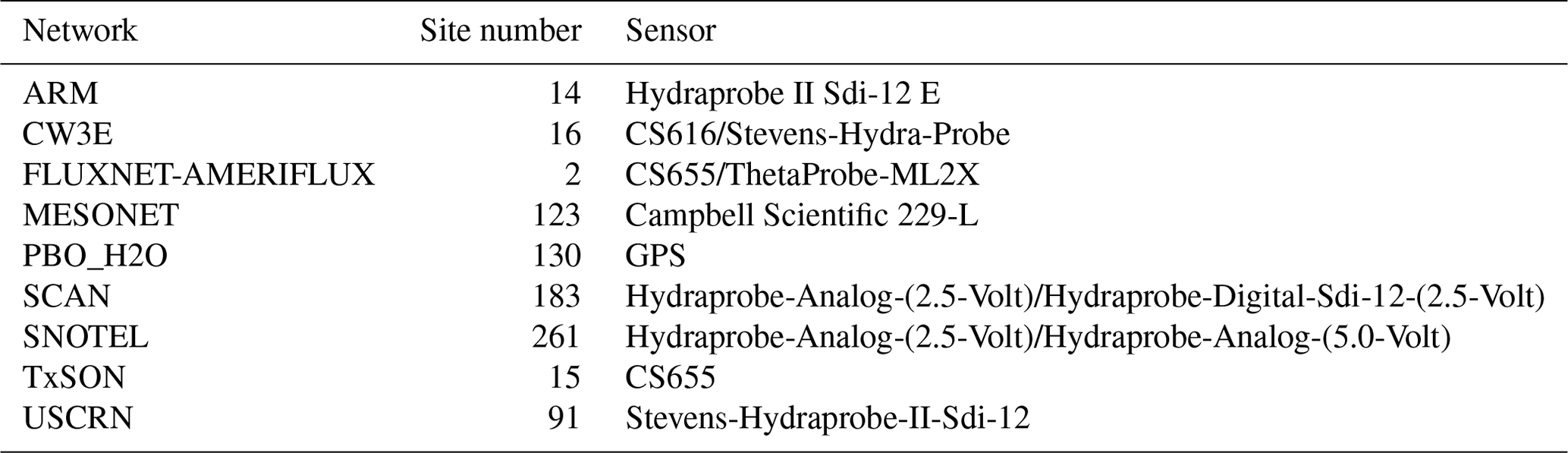
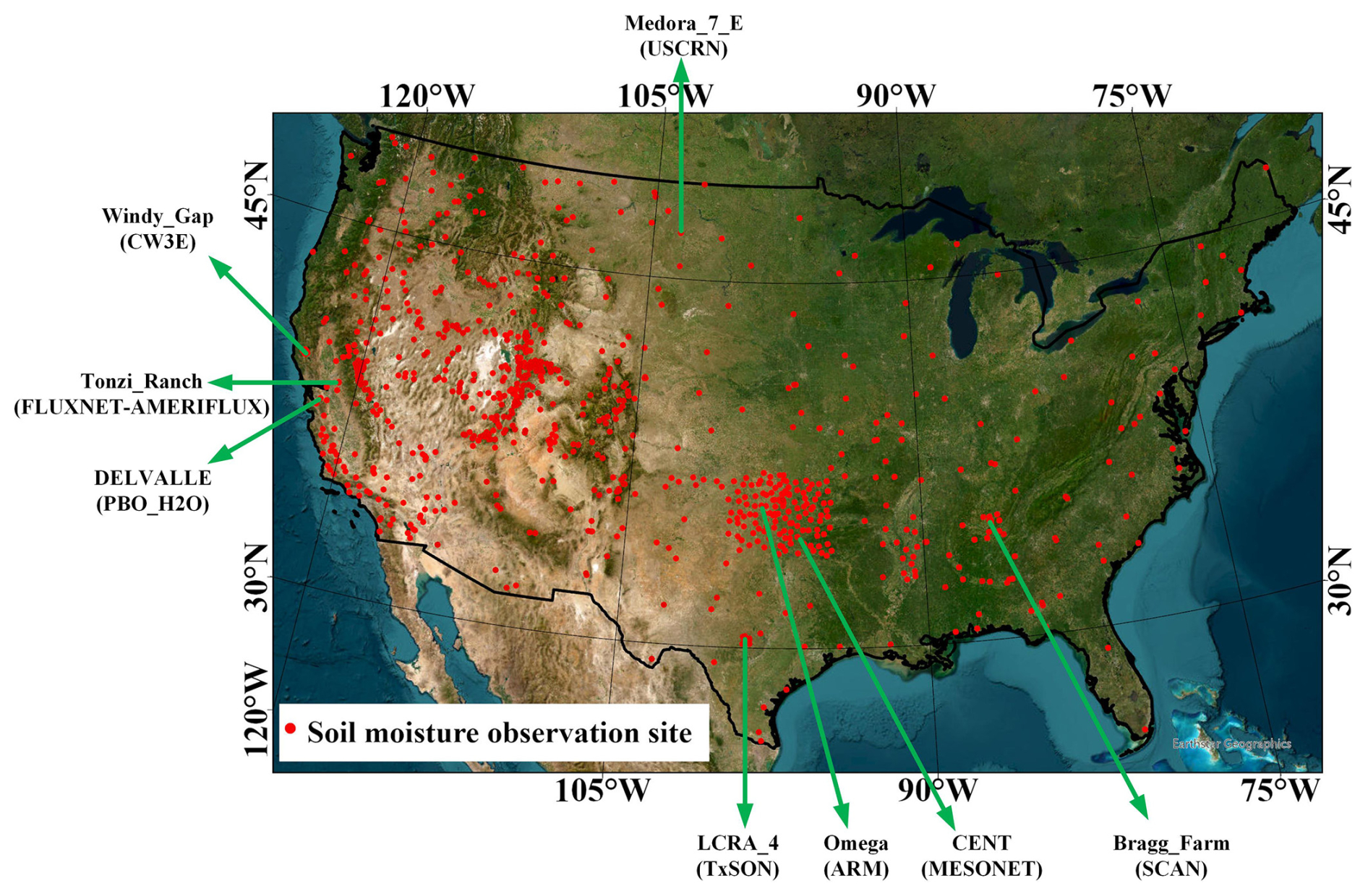
Figure 1 Spatial distribution of the in situ soil moisture observation sites used in this study for soil moisture validation. Each red point refers to one site. The eight marked sites show temporal variations of surface soil moisture (SSM) in Figs. 6 and 7, respectively. The basemap is from Esri, Earthstar Geographics, and the GIS User Community.

2.1.4 Land cover and terrain data

In this study, we validate the performance of our developed datasets for different land cover types and different terrain conditions. Land cover type data were from the National Land Cover Database (NLCD) product available at https://www.mrlc.gov/ (last access: 20 November 2024), which includes annual land cover type at a spatial resolution of 30 m (Homer et al., 2020; Jin et al., 2023). Additionally, 30 m digital elevation models (DEM) from the NASA Shuttle Radar Topography Mission project were utilized to describe the terrain information in the CONUS (Rabus et al., 2003).

2.2 Method

2.2.1 Characteristic extraction

Because of the spatial gaps in the Crop-CASMA SSM data, it is difficult to directly exploit the daily Crop-CASMA SSM scene for the construction of the spatio-temporal fusion model (see next section). To deal with this problem, a time series mining approach, i.e., highly comparative time series analysis (HCTSA), was adopted to extract four spatially seamless 1 km characteristics (maximum, minimum, mean, and median) in each pixel from the Crop-CASMA SSM time series data (Fulcher et al., 2013; Fulcher and Jones, 2017). Additionally, to match the extracted characteristics from the Crop-CASMA SSM data, the same characteristics were also extracted at 9 km resolution from the corresponding SMAP L4 time series data.

Even though the location of spatial gaps in the Crop-CASMA SSM time series are varying over time, the extracted HCTSA-based characteristics are not affected (Yang and Wang, 2023). Typically, some factors that significantly influence SSM (e.g., precipitation, vegetation, and temperature) exhibit periodic changes in the year, indicating that inter-annual fluctuations in SSM tend to follow a periodic pattern. Thus, we selected a 1-year temporal span for extracting these characteristics of maximum, minimum, mean, and median SSM. The extracted characteristics were then utilized to generate the corresponding STF_SSM scene.

2.2.2 Spatio-temporal fusion model

In this study, the virtual image pair-based spatio-temporal fusion (VIPSTF) model is employed to generate the 3 h, 1 km STF_SSM dataset due to its stable performance, superior computational efficiency, and flexible usage (Wang et al., 2020; Yang et al., 2023). The spatial weighting version of the VIPSTF model was adopted in this study because of the reliable accuracy. The operation of the VIPSTF model requires at least one or multiple known image pairs at different spatial resolutions (a data pair is defined as one coarse-resolution and one fine-resolution characteristic extracted from the same year). Here, the extracted 1 and 9 km HCTSA-based characteristics (i.e., maximum, minimum, mean, and median of SSM time series) from the SMAP L4 and Crop-CASMA SSM time series (i.e., four image pairs) are blended using the VIPSTF model. Specifically, each STF_SSM scene is produced as follows:

$$\begin{array}{}\text{(1)}& {\widehat{\mathbf{STF}\mathbf{\_}\mathbf{SSM}}}_t=\mathbf{STF}\mathbf{\_}{\mathbf{SSM}}_{\mathrm{VIP}}+\mathrm{\Delta }\mathbf{STF}\mathbf{\_}{\mathbf{SSM}}_t,\end{array}$$

where ${\widehat{\mathbf{STF}\mathbf{\_}\mathbf{SSM}}}_t$ is the generated 3 h, 1 km SSM scene at time t and ΔSTF_SSM_t refers to the increment data of the model at a 1 km spatial resolution at time t. The virtual STF_SSM_VIP scene was predicted using a linear combination of the four extracted 1 km characteristics from the Crop-CASMA SSM time series data in Eq. (2):

$$\begin{array}{}\text{(2)}& \mathbf{STF}\mathbf{\_}{\mathbf{SSM}}_{\mathrm{VIP}}=\sum _{i=\mathrm{1}}^n{a}_i\mathbf{F}\mathit{\_}{\mathbf{C}}_i+b,\end{array}$$

where a_i is the coefficient for the ith extracted fine characteristic F_C_i at a 1 km spatial resolution. n is the number of the characteristics (n=4 in this study), and b denotes a constant. Based on the assumption of scale invariance (Wang and Atkinson, 2018), the optimal coefficients a_i and b for each 3 h SMAP scene were calculated in a linear regression as follows:

$$\begin{array}{}\text{(3)}& {\mathbf{SMAP}}_t=\sum _{i=\mathrm{1}}^n{a}_i\mathbf{C}\mathit{\_}{\mathbf{C}}_i+b+\mathrm{\Delta }{\mathbf{SMAP}}_t,\end{array}$$

where SMAP_t refers to the known SMAP L4 SSM scene at time t and C_C_i is the ith extracted coarse characteristic at a 9 km spatial resolution from the SMAP L4 SSM time series data. ΔSMAP_t represents the residual data from the regression at time t. Moreover, the increment data (i.e., ΔSTF_SSM_t) in Eq. (1) can be disaggregated by the following spatial weighting scheme:

$$\begin{array}{}\text{(4)}& \mathrm{\Delta }\mathbf{STF}\mathbf{\_}{\mathbf{SSM}}_t(x_{\mathrm{0}},y_{\mathrm{0}})=\sum _{k=\mathrm{1}}^s{w}_j\mathrm{\Delta }{\mathbf{SMAP}}_t(x_k,y_k).\end{array}$$

In Eq. (4), (x_k,y_k) denotes the spatial distribution of the kth similar pixel surrounding the center pixel (x₀,y₀). The number of surrounding similar pixels is represented by s. Additionally, w_j represents a weight calculated based on the distance between the center pixel and the kth surrounding similar pixels. ΔSMAP_t was interpolated from 9 to 1 km using the bicubic method.

2.2.3 Data generation

Based on the VIPSTF model, the 3 h, 1 km STF_SSM dataset was generated from 1 April 2015 to 31 December 2023. The generation flowchart is depicted in Fig. 2. The specific process steps for producing the STF_SSM dataset are described as follows:

1. For each year, 1 and 9 km spatially seamless characteristics (i.e., maximum, minimum, mean, and median) were extracted from the Crop-CASMA and SMAP L4 SSM time series using the HCTSA method, respectively.

2. To generate a STF_SSM scene at time t, a VIPSTF model was constructed using the extracted characteristics in step (1) and a SMAP L4 SSM scene at time t within the year. Then, the STF_SSM scene at time t was generated.

3. The aforementioned steps were repeated after each 3 h period to produce the 3 h, 1 km STF_SSM data.

Finally, a total of 25 567 STF_SSM scenes were produced, accounting for approximately 1.78 TB. Each STF_SSM scene requires approximately 73.0 MB of storage space. The Pete High-Performance Computing (HPC) facility at Oklahoma State University was employed for data generation.

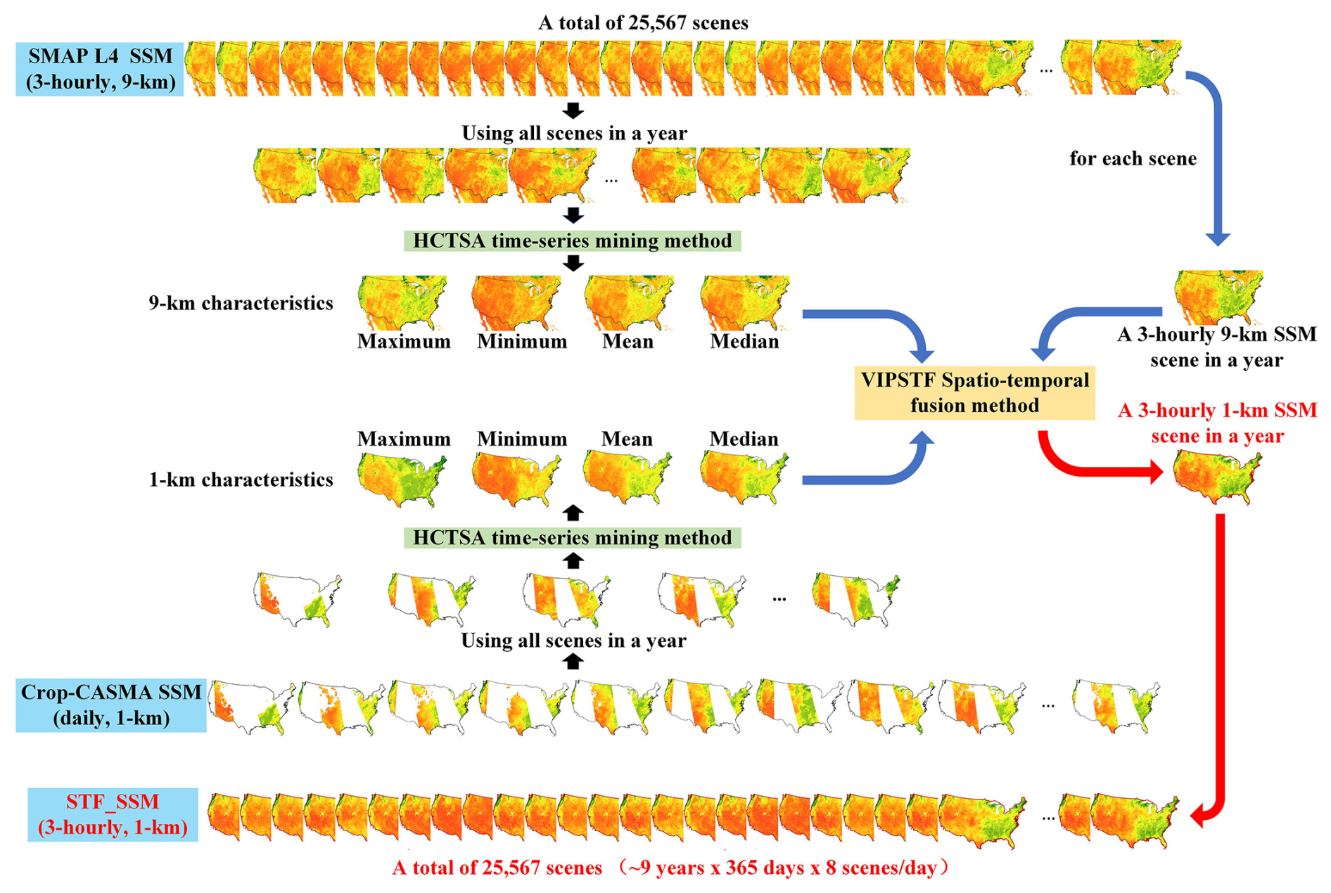
Figure 2 Flowchart for generating the 3 h, 1 km STF_SSM dataset from 2015 to 2023.

2.3 Validation

In this paper, we divide the soil moisture observations (Fig. 1) into two groups (3 h group and daily group) for the validation of our generated data. Considering that the time of SMAP L4 and STF_SSM data is not on the hour (at 01:30, 04:30, 07:30, 10:30, 13:30, 16:30, 19:30, and 22:30 UTC (time zone used throughout)), the average SSM value between two adjacent integer times was used to represent the SSM value at the specific time. For example, when validating the SMAP L4 and STF_SSM scenes at 04:30, the mean value of the 04:00 and 05:00 in situ data was used to represent the soil moisture at 04:30. For daily-scale validation, the hourly in situ data were averaged to obtain daily values. Similarly, the 3 h SMAP L4 and STF_SSM data were composited into daily scenes. To assess accuracy, five widely used statistical metrics were adopted, that is, the correlation coefficient (CC), root mean square error (RMSE), bias (Bias), unbiased root mean square error (ubRMSE), and Kling–Gupta efficiency (KGE).

3 Results

3.1 Spatial pattern of the developed SSM dataset

The spatial pattern of the Crop-CASMA SSM, the SMAP L4 SSM, and the generated STF_SSM datasets are shown in Fig. 3 at four randomly selected time points (i.e., 1 April 2015, 8 June 2017, 16 August 2019, and 25 October 2021). The 1 km Crop-CASMA SSM dataset has spatial gaps and does not have wall-to-wall data covering the entire CONUS. In contrast, both the SMAP L4 and STF_SSM datasets can provide spatially seamless observations. It is noted that the SMAP L4 SSM scenes contain some abnormal pixels with extremely high SSM values (SSM values of 0.6 and higher), especially in the northern part of the CONUS (e.g., some pixels around the Great Lakes in Fig. 3).

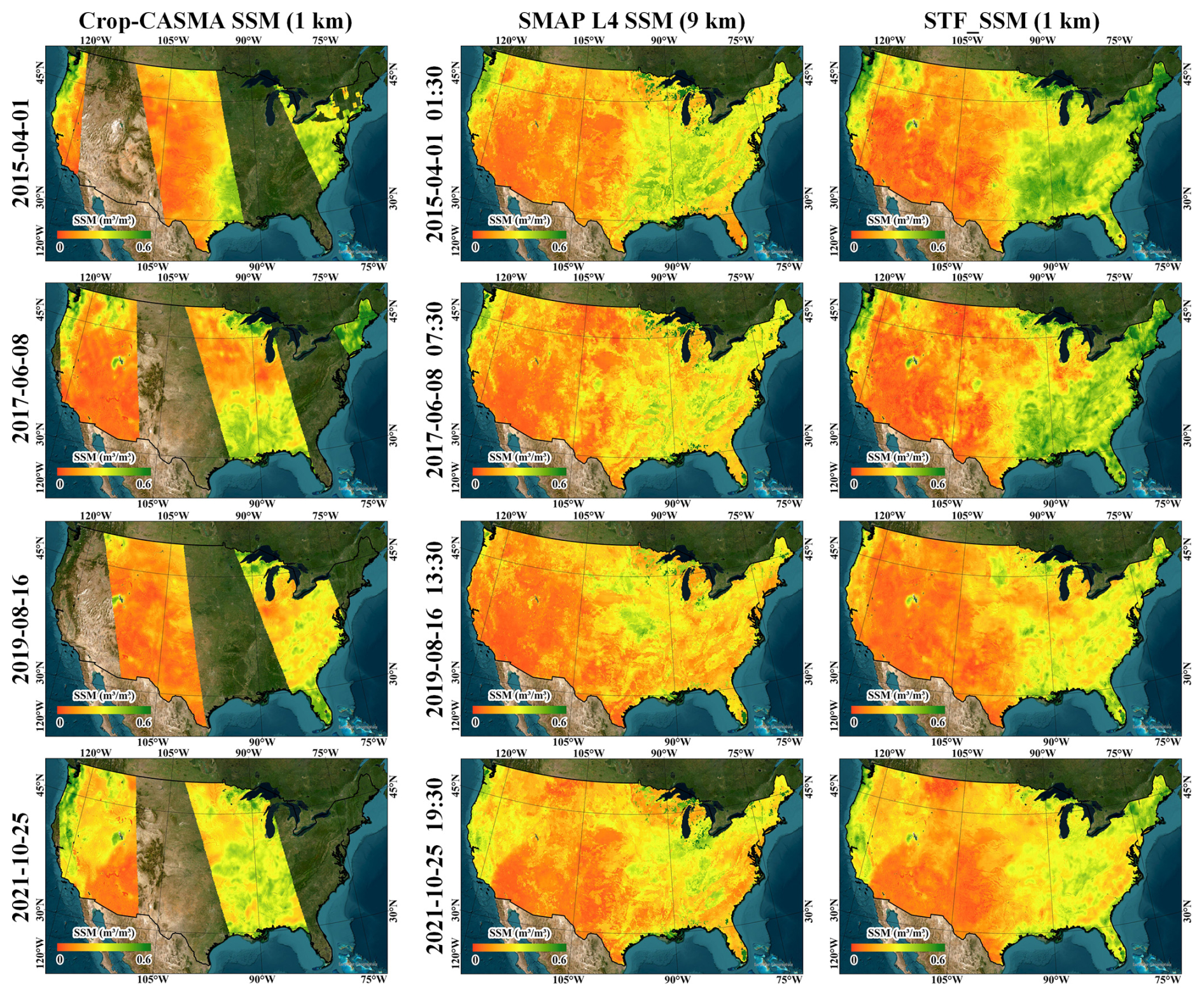
Figure 3 Spatial pattern of surface soil moisture (SSM) in the Crop-CASMA SSM dataset (left), SMAP L4 SSM product (middle), and STF_SSM dataset (right) on 1 April 2015 (01:30), 8 June 2017 (07:30), 16 August 2019 (13:30), and 25 October 2021 (19:30). Both the SMAP L4 and STF_SSM datasets are exhibited at the 3 h scale, while the Crop-CASMA SSM dataset is displayed at the daily scale. The basemap is from Esri, Earthstar Geographics, and the GIS User Community.

To illustrate the advantages of the STF_SSM dataset, we zoomed into a sub-region in the CONUS at a date with rainfall (14 August 2018) and showed SSM in the three different datasets in Fig. 4. It is clear that both the 3 h SMAP L4 SSM and STF_SSM datasets can capture increased SSM values from 01:30 to 07:30 in the southwest region of the sub-region. Moreover, The STF_SSM and Crop-CASMA SSM datasets provide more detailed spatial information than those in the SMAP L4 SSM product. The spatial texture of the STF_SSM dataset closely resembles that of the 1 km Crop-CASMA SSM dataset, which is smoother than that of the SMAP L4 SSM product.

Next, we selected two random pixels in Nebraska (shown in Fig. 4) to exhibit intra-day SSM variation (Fig. 5). Although the Crop-CASMA SSM scene provides spatial information at a 1 km resolution, it only provides the SSM value at the daily scale. In contrast, both the SMAP L4 and STF_SSM datasets show the changes in SSM every 3 h. Furthermore, the changing patterns of SSM over time are similar between the SMAP L4 and STF_SSM datasets (the CC values in Fig. 5a and b are 0.997 and 0.999), indicating the stability and consistency of the STF_SSM dataset.

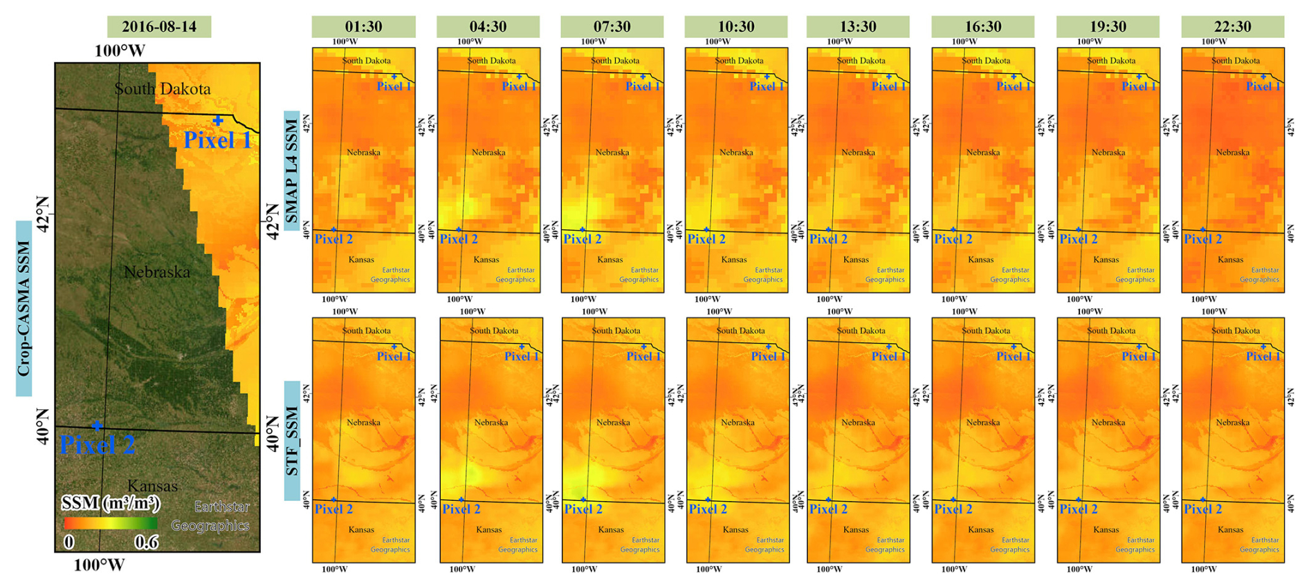
Figure 4 A sub-region in the western continental United States (CONUS) to exhibit the spatial textures of the three surface soil moisture (SSM) datasets on 14 August 2018. The basemap is from Esri, Earthstar Geographics, and the GIS User Community.

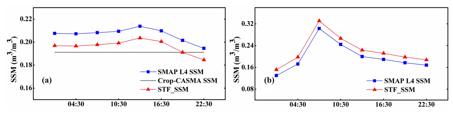
Figure 5 The intra-day surface soil moisture (SSM) variation for two randomly selected pixels on 14 August 2018. The Crop-CASMA SSM dataset does not provide the intra-day SSM variation, shown as the flat black line. Panels (a) and (b) refer to the pixels 1 and 2 in Fig. 4, respectively. Since pixel 2 is located in the spatial gaps of the Crop-CASMA SSM scene, it does not exhibit the flat black line in (b).

3.2 Validation based on daily soil moisture observations

At the daily scale, the three daily SSM datasets (the Crop-CASMA SSM, SMAP L4 SSM, and STF_SSM datasets) were compared against the daily in situ data from nine soil moisture observation networks. Figure 6 shows the SSM time series acquired from four randomly selected sites distributed across the CONUS: the Windy_Gap site in the CW3E network, CENT site in the MESONET network, DELVALLE site in the PBO_H2O network, and LCRA_4 site in the TxSON network. Although there are gaps in the in situ data at these sites, the available in situ data are sufficient for the validation of these three SSM datasets. Moreover, the SSM daily variations of the three SSM datasets are similar to those of the in situ data. For example, the CC values for the SMAP L4, Crop-CASMA, and STF_SSM datasets in Fig. 6a (Windy_Gap site in the CW3E network) are 0.924, 0.879, and 0.886, respectively. In addition, there are some biases between different SSM datasets due to differences in spatial resolution and derived methods. Specifically, the SMAP records a lower minimum SSM value at the Windy_Gap site and a higher SSM maximum at the DELVALLE site compared with the Crop-CASMA and STF_SSM datasets.

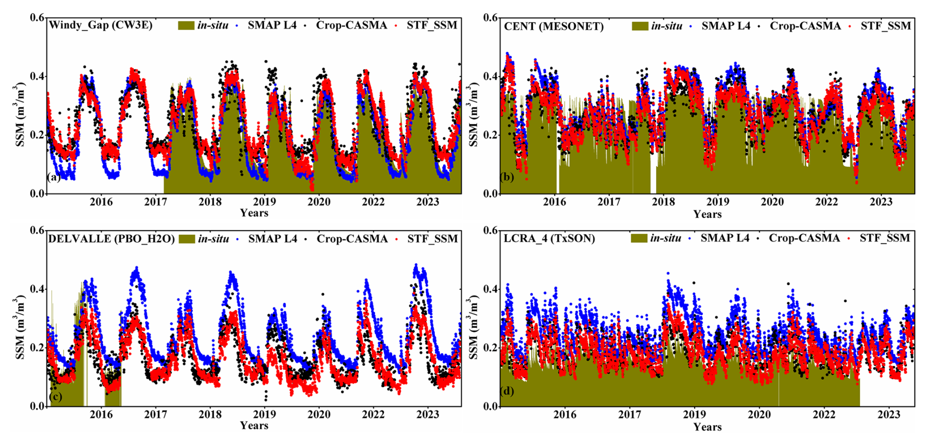
Figure 6 Temporal variations of daily surface soil moisture (SSM) from the SMAP L4 (blue), Crop-CASMA (black), STF_SSM (red), and in situ observation data (dark yellow) at four different sites. (a) Windy_Gap site in the CW3E network. (b) CENT site in the MESONET network. (c) DELVALLE site in the PBO_H2O network. (d) LCRA_4 site in the TxSON network.

Table 2 Accuracy of the daily surface soil moisture (SSM) from the SMAP L4, the Crop-CASMA, and the STF_SSM datasets. Values in bold indicate the dataset with the best performance for each statistic in each row. Underlined values indicate second best.

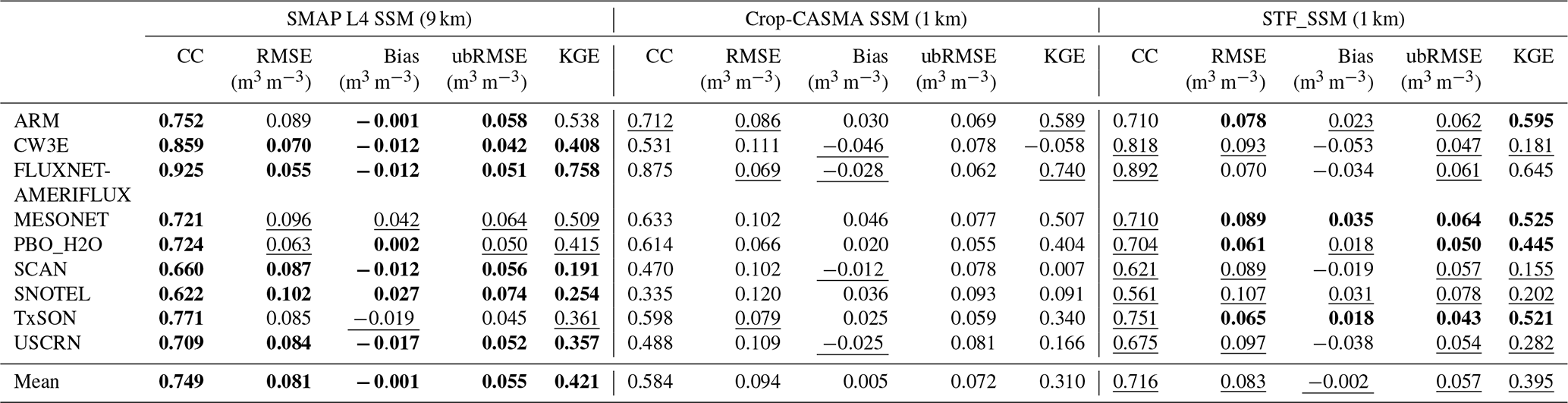
At the network level, the results of the accuracy assessment (Table 2) show that the 9 km SMAP L4 SSM product has the greatest accuracy among the three datasets. At a spatial resolution of 1 km, the generated STF_SSM dataset outperforms the Crop-CASMA SSM dataset. Specifically, the mean CC for the SMAP L4 SSM product is 0.749, which is 0.033 and 0.165 higher than the STF_SSM and Crop-CASMA datasets, respectively. The RMSE and ubRMSE for the SMAP L4 SSM dataset are 0.081 and 0.055 m³ m⁻³ and are the smallest among the three datasets. The STF_SSM dataset has RMSE and ubRMSE values of 0.083 and 0.057 m³ m⁻³ and so are slightly higher than those for the SMAP L4 SSM product but smaller than those for the Crop-CASMA dataset. The Bias for the SMAP L4 SSM product (with a Bias of −0.001 m³ m⁻³) and the STF_SSM dataset (with a Bias of −0.002 m³ m⁻³) are closer to SSM observation data than that of the Crop-CASMA SSM dataset. The STF_SSM dataset has a mean KGE of 0.395, which is 0.026 smaller than that of the SMAP L4 but 0.185 larger than that of the Crop-CASMA dataset. At the three SSM observation networks of MESONET, PBO_H2O, and TxSON, the STF_SSM dataset demonstrates better performance compared to the other datasets. However, for the other networks, the SMAP L4 SSM product outperforms the other datasets in terms of accuracy.

3.3 Validation based on 3 h soil moisture observations

The 9 km SMAP L4 product and the 1 km STF_SSM dataset were compared with the 3 h in situ data from seven networks. We randomly selected four sites (Omega site in the ARM network, Tonzi_Ranch site in the FLUXNET-AMERIFLUX network, Bragg_Farm site in the SCAN network, and Medora_7_E site in the USCRN network) to exhibit the SSM comparison (Fig. 7). The temporal variations of SSM time series from the in situ data, SMAP L4 product, and STF_SSM dataset are similar to each other; e.g., the CC values of the SMAP L4 and STF_SSM datasets in Fig. 7a are 0.749 and 0.745 by referring to the in situ data, revealing that both of the SSM datasets can well capture the dynamics of SSM at the 3 h scale. Moreover, the difference between the 9 km SMAP L4 product and 1 km STF_SSM dataset is small, indicating that the downscaling of our STF_SSM dataset does not introduce significant errors in SMAP L4 SSM. Therefore, our STF_SSM dataset can be regarded as a reliable high-resolution version of the SMAP L4 product.

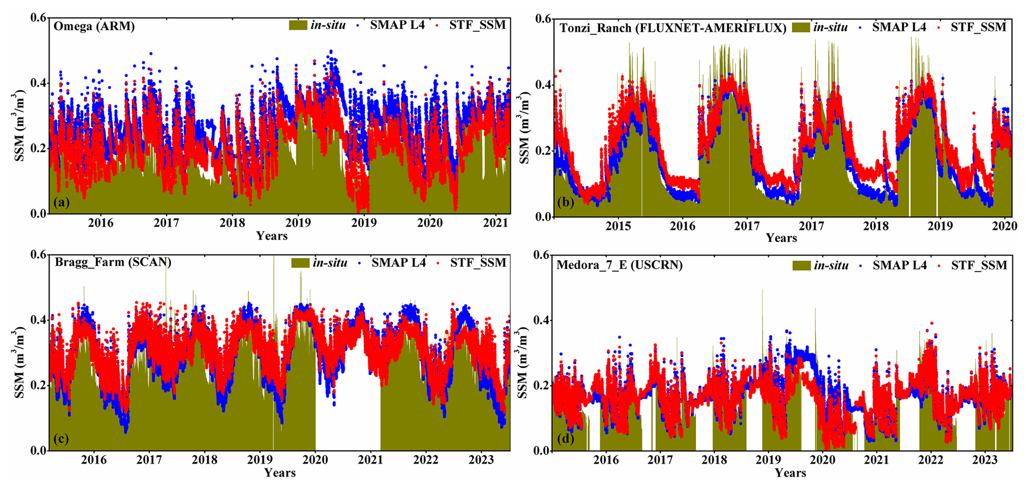
Figure 7 Temporal variations of 3 h surface soil moisture (SSM) from SMAP L4 (blue), STF_SSM (red), and in situ observation data (dark yellow) at four different sites. (a) Omega site in the ARM network. (b) Tonzi_Ranch site in the FLUXNET-AMERIFLUX network. (c) Bragg_Farm site in the SCAN network. (d) Medora_7_E site in the USCRN network.

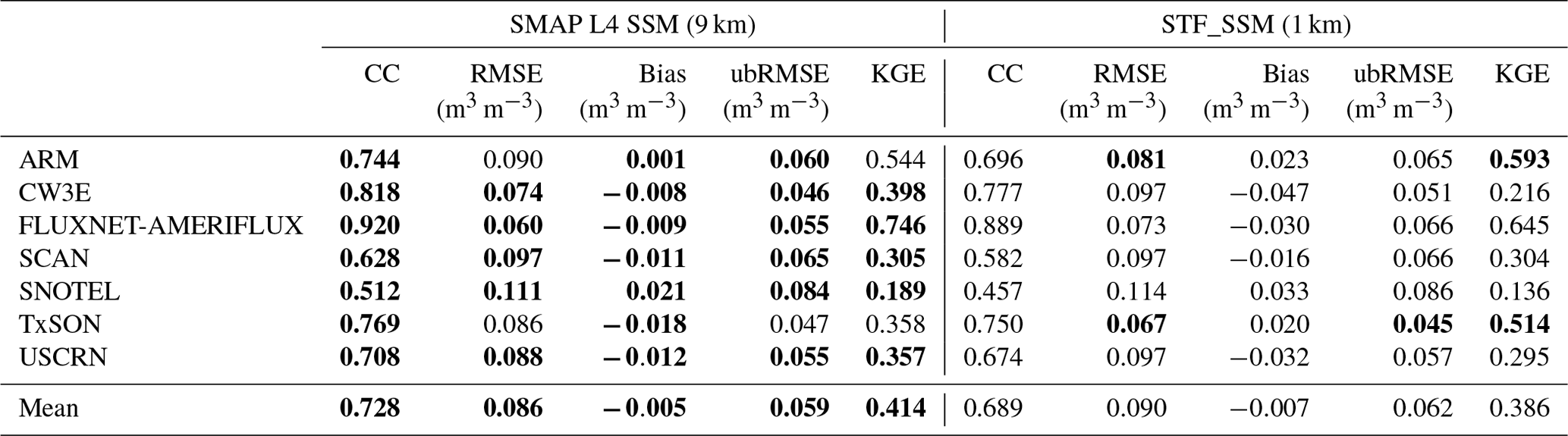
The quantitative statistical metrics based on the 3 h in situ data are listed in Table 3. The results indicate that the 9 km SMAP L4 SSM product has better accuracy than the 1 km STF_SSM dataset. Specifically, the mean CC and KGE for the SMAP L4 SSM product are 0.728 and 0.414, which are values 0.039 and 0.028 higher than those for the STF_SSM dataset. Furthermore, the SMAP L4 SSM product has a mean RMSE and ubRMSE of 0.086 and 0.059 m³ m⁻³. Additionally, the Bias of the SMAP L4 SSM product is −0.005 m³ m⁻³, which is closer to the SSM observation data than that of the STF_SSM dataset. For specific networks, we found that the CC and KGE of the SMAP L4 SSM dataset at the FLUXNET-AMERIFLUX network are 0.920 and 0.889 and therefore are the highest among the seven networks. On the other hand, the STF_SSM dataset provides an RMSE of 0.081 and 0.067 m³ m⁻³ for the ARM and TxSON networks, which is 0.009 and 0.019 m³ m⁻³ lower than the SMAP L4 SSM dataset, respectively.

Table 3 Accuracy of the 3 h surface soil moisture (SSM) from the SMAP L4 SSM product and the STF_SSM datasets. Values in bold indicate the dataset with better performance for each statistic in each row.

3.4 SSM data accuracy across land cover types

Generally, the accuracy of satellite-derived SSM datasets varies between land cover types because the penetration capacity of remote sensing signals can be affected by land cover types. Therefore, it is necessary to assess the performance of the SSM datasets under different land cover types. According to the NLCD land cover product from 2015 to 2023, we separated the CONUS into nine types, that is, developed, barren, forest, shrub, grassland, pasture, crops, wetlands, and changed. The former eight types are the existing categories (e.g., shrub and grassland) or composite categories (e.g., forest is composed of deciduous, evergreen, and mixed forest) in the NLCD product. The changed category refers to the areas where land use has changed between 2015 and 2023.

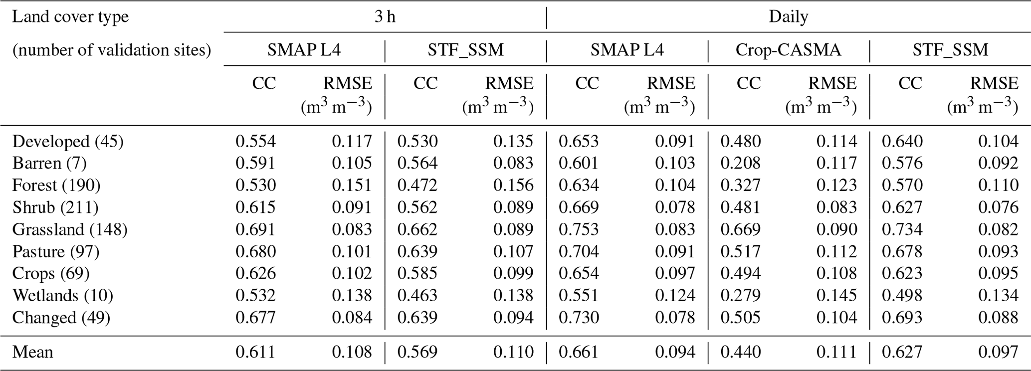
At the 3 h scale, it is seen from Fig. 8a and b that the SMAP L4 product has slightly better performance than the generated STF_SSM dataset for most land cover types. As shown in Table 4, the mean CC and RMSE values of the SMAP L4 product are 0.611 and 0.107 and are 0.042 and 0.002 better than those of the STF_SSM dataset, respectively. However, both SSM datasets exhibit lower accuracy in wetlands compared to other land cover types. Meanwhile, the SSM accuracy has a larger variation across forest pixels, shrub pixels, and developed area pixels than the other land cover types. This is primarily because the topsoil in these land cover types is covered by woody plants and human-made features, which influence SSM observations and lead to a loss of accuracy. The highest accuracy is observed in barren (with an RMSE of 0.083 m³ m⁻³ for the STF_SSM dataset) and grassland areas (with an RMSE of 0.083 m³ m⁻³ for the SMAP L4 product) as these types tend to have less cover. The land cover changes observed in the changed category also provide satisfactory accuracy. This is because approximately 50 % of the land cover change samples consist of barren or grassland areas, which contribute to higher SSM accuracy. These patterns are also reflected in the daily SSM datasets (Fig. 8c and d). Moreover, the Crop-CASMA dataset (with mean CC and RMSE values of 0.440 and 0.111, respectively) has a lower performance than the STF_SSM dataset across all land use covers, highlighting the reliability of the generated STF_SSM dataset at a 1 km spatial resolution.

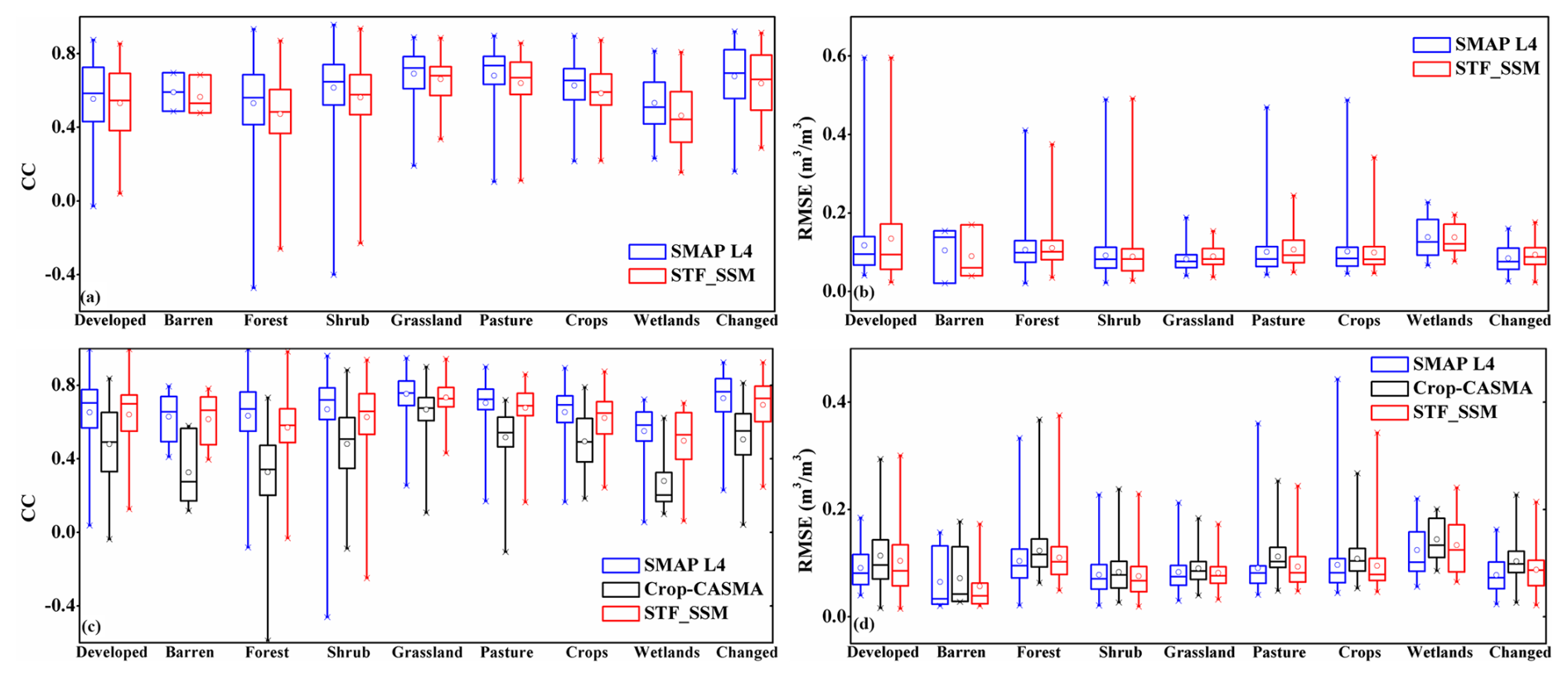
Figure 8 Accuracy of the surface soil moisture (SSM) datasets under different land cover types. The “changed” type refers to areas where land cover type changed between 2015 and 2023. Panels (a) and (b) are the correlation coefficient (CC) and the root mean square error (RMSE) of SSM datasets at the 3 h scale. Panels (c) and (d) are the CC and RMSE of SSM datasets at the daily scale. For each land cover type, the number of validation sites is 45 (developed), 7 (barren), 190 (forest), 211 (shrub), 148 (grassland), 97 (pasture), 69 (crops), 10 (wetlands), and 49 (changed), respectively.

Table 4 Mean correlation coefficient (CC) and root mean square error (RMSE) of surface soil moisture (SSM) datasets under different land cover types.

3.5 SSM data accuracy across topographic conditions

As a significant soil-forming factor, terrain is one of the determinants of SSM variations. Particularly, SSM could have strong spatial variability in areas with complex topographic conditions. We analyzed the accuracy (including CC and RMSE) of the 1 km Crop-CASMA and STF_SSM datasets under different topographic conditions. As shown in Fig. 9a and b, both the Crop-CASMA and STF_SSM datasets show a decrease in the CC value with increasing elevation. However, the STF_SSM dataset shows a slower decline in accuracy (with a slope of −0.055) compared to the Crop-CASMA dataset (with a slope of −0.100). Under complex terrain conditions (i.e., larger slope), the accuracy of both SSM datasets is reduced. It can be seen from Fig. 9c and d that the CC of the Crop-CASMA dataset decreases more sharply as the slope increases (with a slope of −0.023), while the CC in the generated STF_SSM dataset declines more gradually (with a slope of −0.011). Likewise, Fig. 9e and f show that the RMSE values of both SSM datasets increase with elevation. According to the intercept, the STF_SSM dataset has a slightly greater RMSE than the Crop_CASMA dataset, especially at high altitudes. Meanwhile, with an increase in slope, the STF_SSM dataset has a slower rise in RMSE values than the Crop-CASMA dataset (Fig. 9g and h). This suggests that the STF_SSM dataset is more reliable than the Crop-CASMA dataset in complex terrain conditions.

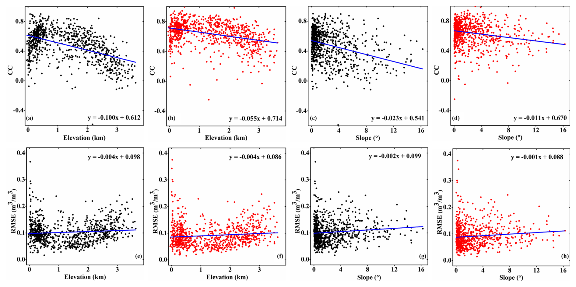
Figure 9 Accuracy of the estimated surface soil moisture (SSM) from the 1 km Crop-CASMA and generated STF_SSM datasets along changing topographic conditions, denoted by elevation and slope. Panels (a), (c), (e), and (g) refer to the 1 km Crop-CASMA SSM dataset. Panels (b), (d), (f), and (h) are the generated STF_SSM dataset.

4 Discussion

4.1 Implications

Ma et al. (2021) adopted the daily 25 km, 10 d composited CCI SSM time series to define agricultural drought events. However, this 10 d composition approach may not capture the rapidly developed drought phenomena (e.g., flash drought). In contrast, the generated 3 h, 1 km STF_SSM dataset has advantages over the CCI dataset because the STF_SSM dataset provides more detailed and continuous SSM information in both the temporal and spatial dimensions. This implies that the STF_SSM dataset can detect both long-term and flash drought events at a finer scale.

Figure 10 exhibits the SSM variation under four drought events in Oklahoma (January to February 2018), Alabama (May to December 2016), California (January to December 2020), and Nevada (January to December 2020) (U.S. Drought Monitor, 2024). The SSM in our dataset shows a clear response to the drought event. As shown in Fig. 10a, during the Oklahoma's drought in early 2018 (Shephard et al., 2021), SSM is about 0.08 m³ m⁻³ lower than the multi-year average value from 2015 to 2023. The drought was gradually alleviated in February. Alabama's drought in 2016 began around May and continued into December (Fig. 10b) (Noel et al., 2020) as the SSM value began to deviate from the average in May and remained in a lower range. In 2020, California and Nevada suffered extreme and long-term droughts (Williams et al., 2022); Fig. 10c and d show that SSM values in the two states were generally lower than the average and continued for the entire year.

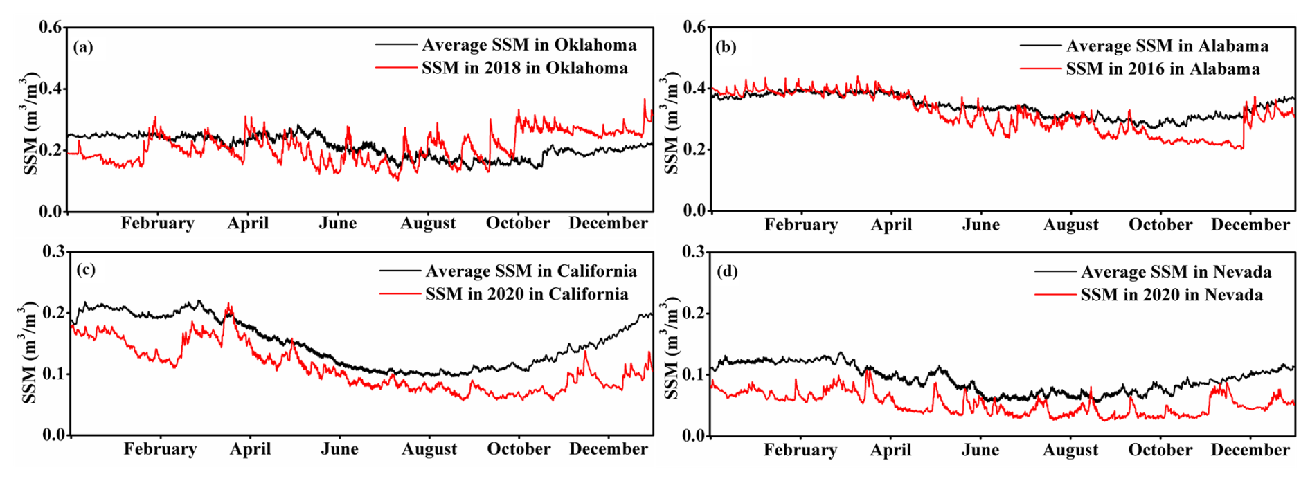
Figure 10 Surface soil moisture (SSM) variations under drought events. Black lines refer to the average SSM values calculated from 2015 to 2023. Red lines represent the SSM values for the corresponding year. (a) The drought in Oklahoma in 2018. (b) The drought in Alabama in 2016. (c) The drought in California in 2020. (b) The drought in Nevada in 2020.

In addition to droughts, SSM is also sensitive to flooding. When a flooding event begins, the SSM value is usually rapidly increased over a short period. To highlight the advantages of the developed 3 h SSM dataset, we portrayed the SSM variation under two flooding events. Figure 11a shows the flooding in 2015 in Williamsburg, South Carolina, because of extreme precipitation from 1 to 5 October 2015. It can be seen that the SSM value in this region began to increase dramatically from the evening of 1 to 2 October 2015 and remained at a high level until 5 October 2015. Figure 11b presents the flooding in 2017 in Jefferson, Texas, due to Hurricane Harvey. We found that the SSM value had started to rise on the evening of 24 August 2017 before Hurricane Harvey reached landfall fully (25 August 2017) and peaked on 27 August 2017.

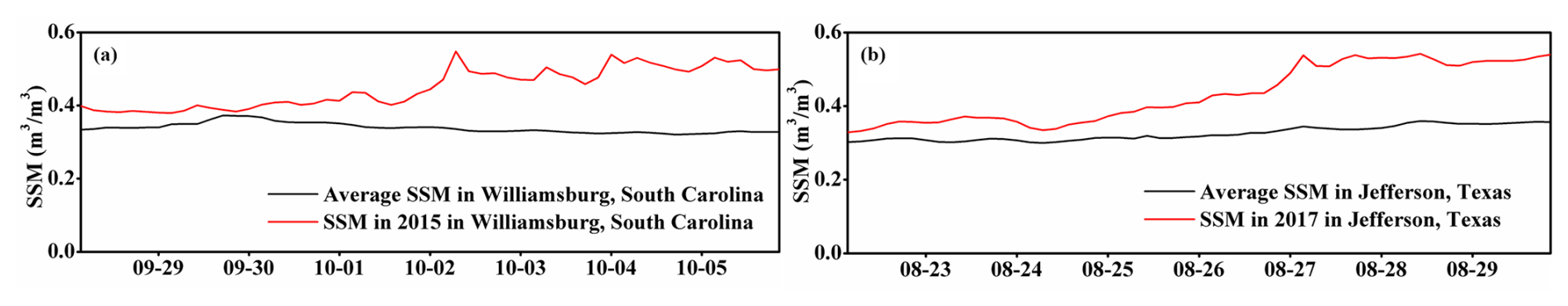
Figure 11 Surface soil moisture (SSM) variations under flood events. Black lines represent the average SSM values calculated from 2015 to 2023. Red lines are the SSM values for the corresponding year. (a) The flood in Williamsburg, South Carolina, in 2015. (b) The flood in Jefferson, Texas, in 2017.

It is clear from the mentioned analysis that SSM information is closely linked to drought and flooding. This suggests that SSM can be applied to identify these events and quantify their severity. Thus, the developed STF_SSM dataset has great potential for application, especially in agriculture. For instance, near-real-time crop conditions could be observed directly by dynamically monitoring SSM. It will provide a rational basis for refining irrigation management. In addition, severe drought and flooding affect crop yields, implying that SSM information with fine spatio-temporal resolution also has the potential to play an important role in crop yield estimation.

4.2 Accuracy and latency time of updated STF_SSM data

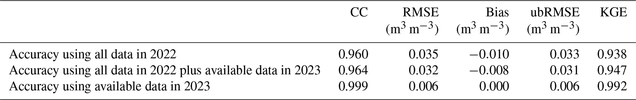
Drought monitoring needs real-time or near-real-time soil moisture data and requires high data accuracy and short latency time. Since the strategies of characteristic extraction for training the STF_SSM dataset from 2015 to 2023 depend on the complete SSM time series data over the entire year, it is difficult to directly update the near-real-time data using this strategy. Therefore, we propose three alternative strategies for characteristic extraction to examine on a randomly selected date in 2023 (10 January 2023). This first alternative is using all data in 2022, the second alternative is using available data in 2023 (before 10 January 2023), and the third is using all data in 2022 plus available data in 2023. By referring to the corresponding STF_SSM scenes (predicted using all data in 2023), we found that using available data in 2023 has the greatest performance among the three strategies of characteristic extraction with a mean CC and RMSE of 0.999 and 0.006 m³ m⁻³ (Table 5). Meanwhile, the CC and KGE of using all data in 2022 plus available data in 2023 are 0.964 and 0.947 and so are 0.004 and 0.009 higher than those using data only in 2022. This means that using characteristics extracted from temporally adjacent data in 2023 improves fusion accuracy.

Due to a data-driven approach to production, real-time updates of the STF_SSM data have unavoidable latency time. This is because the latency time of the STF_SSM dataset depends on that of other auxiliary data. According to the investigation from the official website, the near-real-time SMAP L4 SSM product and Crop-CASMA SSM dataset usually have 3 and 2 d of latency, respectively. Thus, if only available data within the year are adopted to update the STF_SSM data, the latency time of the near-real-time STF_SSM scene is at least 3 d.

Table 5 Accuracy of near-real-time STF_SSM data (on 10 January 2023) production using different strategies of characteristic extraction.

4.3 Analysis of different fine SSM datasets

Currently, some high-resolution SSM datasets have been published and used. We listed six 1 km SSM datasets at a large scale and exhibited the details of these datasets, such as the spatial resolution, temporal resolution, and accuracy, in Table 6. Given the differences in validation methods, spatial and temporal coverages, and statistical metrics, etc., it is difficult to harmonize these datasets to the same standard to quantify accuracy. Therefore, before using the data, it is necessary to further select the more suitable SSM dataset according to the requirements.

Table 6 Comparative analysis for six high-resolution SSM datasets. Statistical metrics for accuracy include the root mean square error (RMSE), unbiased root mean square error (ubRMSE), and unbiased root mean square deviation (ubRMSD).

4.4 Uncertainties and future works

Although the STF_SSM dataset has good performance in representing the fast changes in soil moisture, two uncertainties in the data generation need to be noted. First, the spatio-temporal fusion model used in this study is a data-driven method which depends on the stable and accurate SMAP L4 SSM product and Crop-CASMA SSM dataset. If either of these datasets stops updating or contains significant errors, the generation and accuracy of the STF_SSM dataset will be impacted. Second, many environmental and ecological variables affect the SSM, such as precipitation, vegetation, temperature, evaporation, and terrain. However, these variables are not fully considered in the STF_SSM production, decreasing the interpretability of the STF_SSM dataset.

Currently, geostationary satellites have a large potential to provide hourly and spatially fine auxiliary variables to produce SSM datasets. Fusing the auxiliary variables from the geostationary satellites for the generation of hourly SSM data is an ongoing work. However, the extensive data acquisition and necessary preprocessing steps can significantly increase the time cost of data production without leading to a substantial improvement in accuracy. Thus, balancing data accuracy and generation efficiency is necessary for the downscaling of the SSM dataset in the future. Compared with existing SSM datasets, the generated SSM dataset in this study has advantages in terms of spatio-temporal resolution. It is worthwhile to further explore its potential applications, such as monitoring drought severity and occurrences, quantifying wildfire danger levels, evaluating responses of agriculture and natural ecosystems to soil moisture dynamics, and understanding local and regional hydrological processes.

5 Code and data availability

The STF_SSM dataset is available at https://doi.org/10.5066/P13CCN69 (Yang et al., 2025a). Moreover, the STF_SSM dataset and generating code are also published at https://doi.org/10.6084/m9.figshare.28188011 (Yang et al., 2025b).

6 Conclusions

In this study, we develop a spatio-temporal fusion model to generate the first spatially seamless 3 h, 1 km STF_SSM dataset in the CONUS from 2015 to 2023. This dataset integrates the 3 h, 9 km SMAP L4 SSM product from NASA and the daily, 1 km Crop-CASMA SSM dataset from USDA-NASS. The former provided fine temporal resolution, and the latter provided detailed spatial details. To deal with the mismatch between the two datasets in terms of temporal resolution and spatial coverage, the HCTSA-based time series mining method was used to extract spatially seamless characteristics from both SSM time series data for each year. Four characteristics extracted at 1 and 9 km spatial resolutions (minimum, maximum, mean, and median of SSM time series) were employed as inputs of the fusion model. By coupling with each 3 h, 9 km SMAP L4 scene, the downscaled 3 h, 1 km STF_SSM scene was simulated in turn. Data validation at the daily scale showed that the generated 1 km STF_SSM dataset (with a mean CC and ubRMSE of 0.716 and 0.057 m³ m⁻³) outperforms the 1 km Crop-CASMA SSM dataset (with a mean CC and ubRMSE of 0.584 and 0.072 m³ m⁻³) when compared to in situ measurements. At the 3 h scale, the accuracy of the 9 km SMAP L4 SSM product (with a mean CC and ubRMSE of 0.728 and 0.059 m³ m⁻³) is slightly higher than that of the 1 km STF_SSM dataset (with a mean CC and ubRMSE of 0.689 and 0.062 m³ m⁻³). Additionally, the STF_SSM dataset has a better performance than the Crop-CASMA dataset under complex terrain conditions. Overall, the generated 3 h, 1 km STF_SSM dataset is reliable and has great potential for applications at various spatio-temporal scales. The proposed STF_SSM dataset can be freely acquired from https://doi.org/10.5066/P13CCN69 (Yang et al., 2025a).