An integrated high-resolution bathymetric model for the Danube Delta system

Acting as a buffer between the Danube and the Black Sea, the Danube Delta plays an important role in regulating the hydro-biochemical flows of this land–sea continuum. Despite its importance, very few studies have focused on the impact of the Danube Delta on the different fluxes between the Danube and the Black Sea. One of the first steps in characterizing this land–sea continuum is to describe the bathymetry of the delta. However, there are no complete, easily accessible bathymetric data on all three branches of the delta to support hydrodynamic, biogeochemical, or ecological studies. In this study, we aim to fill this gap by combining four different datasets, three in the river and one for the riverbanks, each varying in density and spatial distribution, to create a high-resolution bathymetry dataset. The bathymetric data were interpolated on a hybrid curvilinear–unstructured mesh with an anisotropic inverse distance weighting (IDW) interpolation method. The resulting product offers resolutions ranging from 2 m in a connection zone to 100 m in one of the straight unidirectional channels. Cross-validation of the dataset underlined the importance of the data source spatial pattern, with average root mean square errors (RMSEs) of 0.55 %, 6.3 %, and 27.6 % for river segments covered by the densest to coarsest datasets. These error rates are comparable to those observed in bathymetry interpolation in rivers with similar source datasets. The bathymetry presented in this study is the first unique, high-resolution, comprehensive, and easily accessible bathymetric model covering all three branches of the Danube Delta. The dataset is available at https://doi.org/10.5281/zenodo.14055741 (Alaerts et al., 2024).

1 Introduction

The Danube, Europe's second-longest river, flows through 10 countries and drains an extensive catchment area of ∼800 000 km² before emptying into the Black Sea, where it is the primary source of water and nutrients. About 110 km before reaching the coast, the river splits into three main branches: the Chilia, Sulina, and Sfantu Gheorghe branches (Fig. 1). Between these three branches, spanning ∼5000 km², lies the Danube Delta (Romanescu, 2013; Bănăduc et al., 2023; Driga, 2008). The Danube Delta is a complex system of lakes, channels, and flood plains. It acts as a crucial buffer zone for water, nutrients, and sediments between the Danube and the Black Sea (Sommerwerk et al., 2023; Cristofor et al., 1993; Suciu et al., 2002). The delta is also a biodiversity hotspot and has substantial importance for local inhabitants, providing essential resources for drinkable water, fishing, aquaculture, agricultural lands, transport, and recreational activities (Bănăduc et al., 2016, 2023; Lazar et al., 2022).

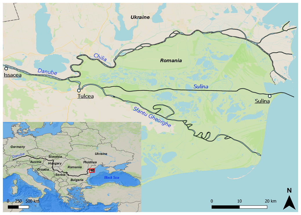
Figure 1 Map of the Danube Delta. The zoomed-out view (bottom left panel) displays the countries through which the Danube flows, with the river represented by a black line. The red rectangle outlines the area covered by the close-up view. In the close-up view of the delta, the black line marks the boundaries of the zone of interest, while the dashed line indicates the national borders. The basemaps are the Ocean Basemap (Esri, 2018) for the zoomed-out view and the Voyager map tile by CartoDB for the close-up view (CC BY 3.0). Data from OpenStreetMap © contributors 2019. Distributed under the Open Data Commons Open Database License (ODbL) v1.0.

Of the three branches, Chilia is the northernmost and serves as a natural boundary between Ukraine and Romania. It is the youngest and least transformed of the three branches and includes numerous meanders and islands. It splits into four smaller branches before reaching the sea, creating a secondary delta within the Danube Delta (Romanescu, 2013; Bănăduc et al., 2023). The Sulina branch is located in the centre of the delta. It is the shortest and most altered by anthropogenic activities of the three branches. The rectification of the branch, during a so-called “cut-off” programme, took place at the end of the 19th century and greatly impacted the path and discharge of the Sulina branch, now linking the cities of Tulcea and Sulina in an almost straight line. The branch is the main shipping route of the delta (Panin and Jipa, 2002; Driga, 2008; Duţu et al., 2018). Sfantu Gheorghe is the southernmost branch. Like the Chilia branch, it meanders a lot, but another cut-off programme was carried out in the 1980s to rectify all of the meander bends, shortening the total length of the branch (Panin and Jipa, 2002).

Despite its ecological and socio-economic importance, comprehensive studies on the delta dynamics and ecological status as a whole are scarce. In terms of bathymetry, some studies have focused on specific channels (Roşu et al., 2022; Jugaru Tiron et al., 2009) and broader campaigns have covered entire branches (Duţu et al., 2018; DDNIRD, 2015). There is however no publicly available bathymetry product covering the entirety of the three branches to support hydrodynamic, biogeochemical, or ecological studies on the Danube Delta as a whole. Bathymetry plays an important role in the description of aquatic environments. Overly coarse resolution or poor-quality bathymetric data can result in substantial errors in predicting water column heights, flood extents, velocities, and shear stress. In larger systems like deltas and estuaries, these inaccuracies can substantially affect the distribution of water (Dey et al., 2022; Fuchs et al., 2022; Merwade et al., 2005).

Our goal in this study is to produce a complete bathymetry model of the three branches of the Danube Delta, from the city of Issacea to the Black Sea (Fig. 1). To achieve that objective, we will use four different datasets that will be interpolated on a hybrid curvilinear–unstructured mesh. The resulting product will subsequently be used in hydrodynamic models to better represent the role of the delta within the Danube–Black Sea–land continuum.

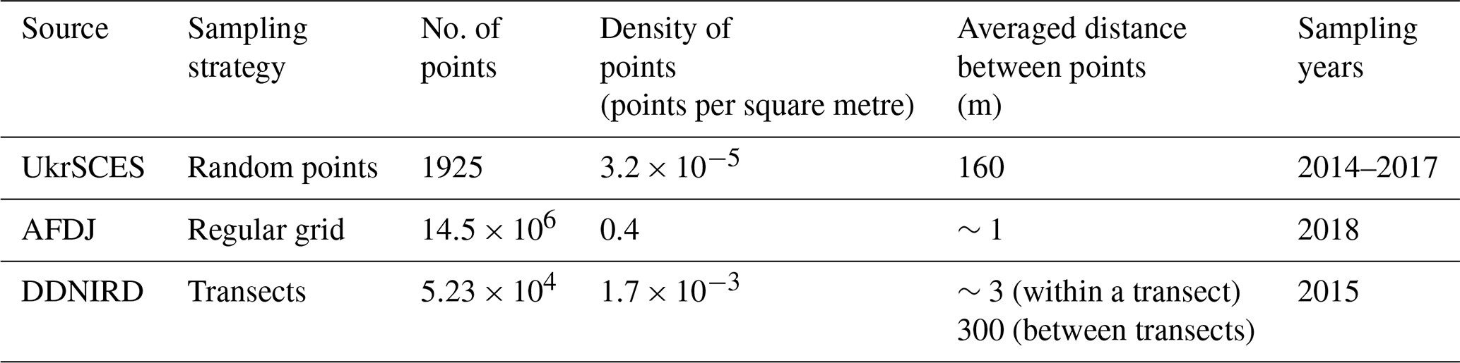
Table 1 Characteristics of the different bathymetric data sources within the river.

2 Data and methods

2.1 Data sources

We used data from four different sources. The first source is the Copernicus digital elevation model (DEM) (European Space Agency, 2021). We used it to determine the riverbanks' positions and heights. It has a resolution of 30 m, and the data date from 2021. The other three sources describe the bathymetry inside the river (Table 1). For the section of the Danube upstream of the delta and the Chilia branch (represented in yellow in Fig. 2), the data come from measurements made by the Ukrainian Scientific Center of Ecology of the Sea (UkrSCES, https://sea.gov.ua/index.php/2016/07/28/about-ukrsces/?lang=en, last access: 18 March 2025) between 2014 and 2017. The data points were collected without adhering to a specific sampling pattern, resulting in variable distances between points and inconsistent sampling density (Fig. 2b). The averaged distance between two points is 160 m but can decrease to ∼50 m. With 1925 data points, this dataset has an averaged point density of $\mathrm{3.2}\times {\mathrm{10}}^{-\mathrm{5}}$ points per square metre, which is rather low compared to the datasets used in other studies (Merwade, 2009; Legleiter and Kyriakidis, 2008; Liang et al., 2022). The section upstream of the Sulina–Sfantu Gheorghe separation and the Sulina branch (Fig. 2c) is covered by data from the Galati Lower Danube River Administration (AFDJ, https://www.afdj.ro/en, last access: 18 March 2025). These data are composed of measurements made on a regular grid of ∼1 m resolution and date from 2018. This dataset is composed of 14.5×10⁶ points, which gives a data point density of 0.4 points per square metre, which is a very high density for a bathymetric survey (Merwade, 2009; Legleiter and Kyriakidis, 2008; Liang et al., 2022). Data for the Sfantu Gheorghe branch come from the Danube Delta National Institute for Research and Development (DDNIRD, https://ddni.ro/wps/, last access: 18 March 2025) (DDNIRD, 2015). These data are composed of transects spaced 300 m apart on average (Fig. 2d). The distance between two points within each transect is ∼3 m. The measurement campaign was carried out in 2015. There are 5.23×10⁴ points in this dataset, and the point density is $\mathrm{1.7}\times {\mathrm{10}}^{-\mathrm{3}}$ points per square metre. This density is in the lower range of what is normally observed in bathymetry interpolation studies (Merwade, 2009; Legleiter and Kyriakidis, 2008; Liang et al., 2022). Due to data scarcity in the region, it was impossible to obtain bathymetric data of the same year for the entire domain.

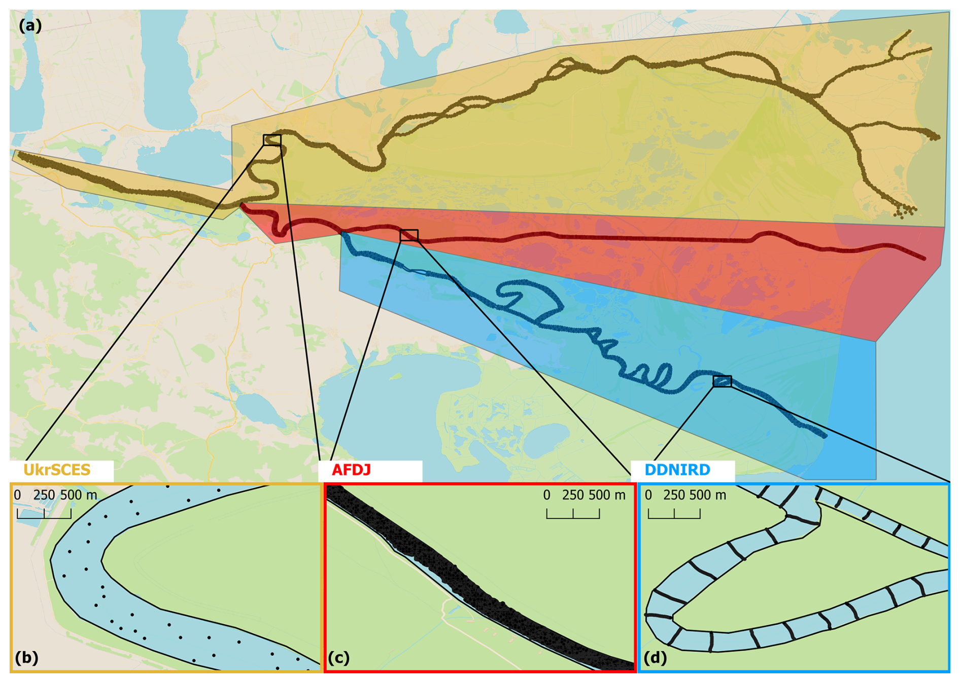
Figure 2 (a) Distribution of the bathymetry sources within the delta. Each colour represents a different source: UkrSCES in yellow, AFDJ in red, and DDNIRD in blue. Each black dot represents an individual bathymetric data point. (b–d) The bottom three panels provide close-up views at the same scale, displaying the bathymetry sampling points and highlighting the variations in sampling density among the three distinct bathymetry sources. The background image is the Voyager map tile by CartoDB (CC BY 3.0). Data from OpenStreetMap © contributors 2019. Distributed under ODbL v1.0.

2.2 Bathymetry interpolation

Given the diverse data sources, a certain degree of standardization was necessary. First, we had to transition most of the data from their local vertical datum to the WGS84 vertical datum. The UkrSCES data were referenced to the Odessa datum, which is 0.17 m below the WGS84 vertical datum. For the AFDJ data, most of the Sulina channel was referenced to the Marea Neagra Sulina datum, 0.03 m above WGS84, while data upstream of Tulcea and the beginning of the Sulina channel used the Tulcea datum 0.33 m above WGS84. The DDNIRD data were referenced to the Marea Neagra 75 datum, 0.25 m above WGS84 (Anastasiu, 2014).

To merge the different bathymetry sources into a unified bathymetry product, a grid spanning the entire delta is required. In this study, we used a hybrid curvilinear–unstructured mesh (Fig. 3). The mesh consists of quadrilateral elements elongated along the flow in the unidirectional river segments (Fig. 3b and d), combined with unstructured triangular elements in the connection zones between segments (Fig. 3c). This configuration provides an accurate representation of both the river's course and the bottom topography while minimizing disk space requirements (Lai, 2010; Bomers et al., 2019). As the mesh elements adapt to follow the shape of the river, the resolution is not constant. Perpendicular to the river, resolution varies between 2 and 12 m, with an average of 5 m. Along the river, element sizes range from 37 to 102 m, averaging 52 m. In the connection zones, smaller elements are used, ranging from 2 to 9 m with an average resolution of 5 m. Overall, mesh resolution varies from 2 m (in a connection zone) to 102 m (on an edge along the riverbank). Further details of the mesh construction can be found in Appendix A.

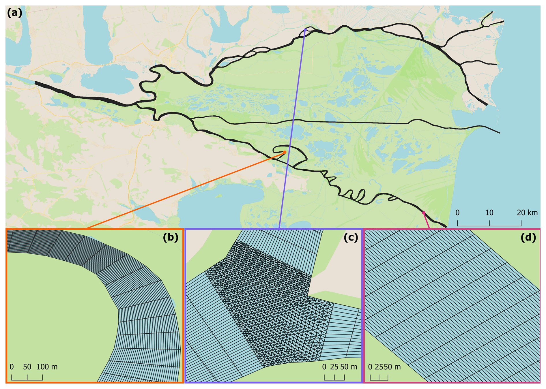
Figure 3 (a) Illustration of the hybrid curvilinear–unstructured mesh on the Danube, with zooms on (b) a bend in the river followed by a narrowing of the river, (c) a connection zone between segments with its unstructured meshing, and (d) a straight portion of the river. The background image is the Voyager map tile by CartoDB, under CC BY 3.0. Data from OpenStreetMap © contributors 2019. Distributed under ODbL v1.0.

The data were then interpolated onto the generated mesh. Interpolation in river systems presents unique challenges due to their inherent anisotropy: bathymetric variations tend to be more pronounced across the river than along its course. To address this, most present-day methods involve projection onto a channel-centred coordinate system, often referred to as an s–n coordinate system or curvilinear coordinate system. In this system, s either represents the centre line or thalweg of the river and n its perpendicular. Further explanations of the projection can be found in Appendix B. Once the bathymetric data are projected onto the s–n coordinate system, an anisotropic interpolation is performed. In this study, we chose an anisotropic inverse distance weighting (IDW) interpolation method, as it is easy to implement and has shown good results in previous studies (Merwade et al., 2006; Diaconu et al., 2019; Liang et al., 2022). Each unidirectional river segment was assigned its own s–n coordinate system, and interpolation was performed segment by segment. To ensure smooth transitions between adjacent segments, the connection zones were included in the projection and interpolation processes of each of their neighbouring segments. As a result, each point in the connection zones was assigned multiple bathymetry values, which were then combined using a weighted mean, with weights inversely proportional to the distance from the corresponding segment. Further details of the interpolation method can be found in Appendix B.

2.3 Validation

2.3.1 Cross-validation

The lack of data in the Danube Delta means that there was no independent dataset to validate our bathymetry product. As a result, we chose to use a “leave-one-out” cross-validation technique (Wu et al., 2019; Liang et al., 2022). In this method, one observation point is iteratively removed, and the interpolation is applied to estimate the bathymetry at that location. The estimated value is then compared to the actual observed data, and this process is repeated for each point in the dataset. We chose this technique because it is best suited for datasets with low point densities where every observation point is valuable. This is however time-consuming since the process has to be repeated for each point of the dataset. This becomes particularly challenging with very large datasets, like the one from AFDJ, which contains 14.5×10⁶ data points. To counter this problem, we chose to use a randomly selected subset of the points where the number of points is too high. As the validation is done segment by segment, we took a random sample of 1000 points for every segment that is covered by more than 1000 data points. In segments with fewer than 1000 points, all of the points were used. Errors in the connection zones were calculated separately from those in the segments. The error metrics we used in the validation are the root mean square error (RMSE) and the relative root mean square error (RRMSE):

$$\begin{array}{}\text{(1)}& {\displaystyle }& {\displaystyle }\mathrm{RMSE}=\sqrt{{\displaystyle \frac{\mathrm{1}}{n}}\sum _{i=\mathrm{1}}^n{\left(z_{\mathrm{obs},i}-z_{\mathrm{predicted},i}\right)}^{\mathrm{2}}},\text{(2)}& {\displaystyle }& {\displaystyle }\mathrm{RRMSE}={\displaystyle \frac{\mathrm{RMSE}}{\frac{\mathrm{1}}{n}\sum _{i=\mathrm{1}}^n{z}_{\mathrm{obs},i}}}\times \mathrm{100}\mathit{\%},\end{array}$$

where i=1, … n are the n points tested on the segment, z_obs,i represents the observed value at the ith point, and z_predicted,i represents the interpolated bathymetry at the same point. The error in the connection was computed separately from the error in the segments in order to be able to find the optimum combination method in the connection zone.

2.3.2 Comparison with global models

At present, there is no unique high-resolution bathymetry dataset easily available for the Danube Delta. In areas where such data are lacking, hydrodynamic models can use global bathymetry models as an alternative. To ensure that the bathymetry product developed in this study offers a clear improvement over existing resources, we compared it against two widely used global bathymetry models: ETOPO 2022 (NOAA National Centers for Environmental Information, 2022) and GEBCO 2024 (GEBCO Bathymetric Compilation Group, 2024). Both models provide bathymetric data on a global scale, delivered on a grid with a resolution of 15 arcsec (∼330 m).

3 Bathymetry product

The final bathymetry product of this study covers the three main branches of the Danube Delta, including all of the channels and meanders for which data were available, from Issacea to the Black Sea (Fig. 4). Detailed views of the three areas, each covered by a different bathymetric data source, demonstrate the consistency between the interpolation and the observed data (Fig. 4b–d). The dataset includes over 5.8×10⁵ points. The bathymetry values range from −3.4 m (negative values indicate points above the reference level) on a dike to 38.8 m in the river near Tulcea, with an average depth of 8.2±5.06 m.

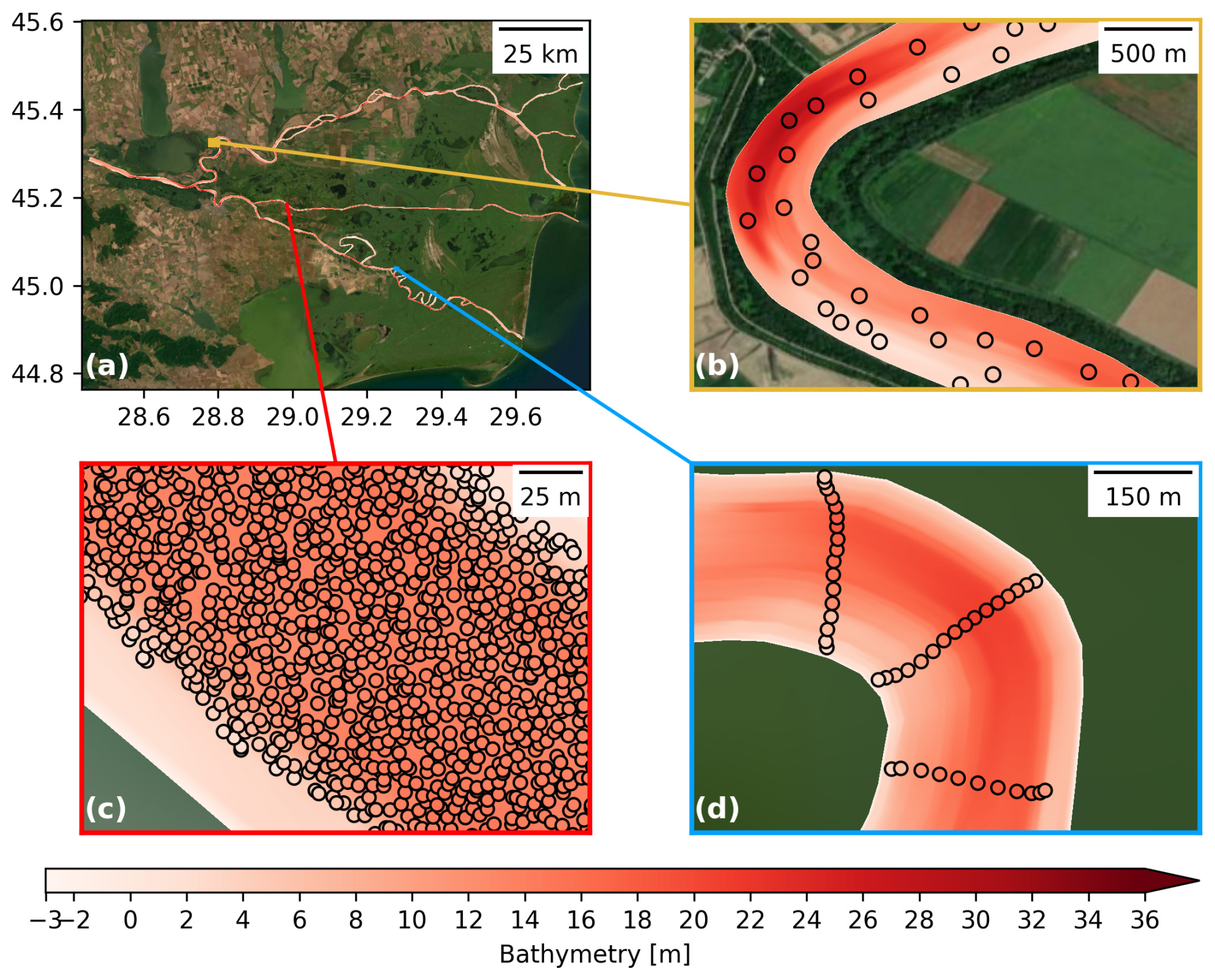
Figure 4 (a) Map of the interpolated bathymetry in the Danube Delta, with close-up views (b–d) showing the interpolated bathymetry in the background and observations as coloured dots. The modelled and observed bathymetries share the same colour bar in all of the panels. (b) Close-up of the Chilia branch. (c) Close-up of the Sulina branch, where the observation data have been resampled to display $\mathrm{1}/\mathrm{15}$ of the points for clarity. (d) Close-up of the Sfantu Gheorghe branch, where the observation data have been resampled to display one-seventh of the points for clarity. The background image is the Esri World Imagery basemap (ESRI, 2025).

Our results align with general river morphology. The bathymetry displays anisotropic patterns, with more pronounced depth variations across the river than along its flow (Fig. 4b–d). Greater depths are observed at the centres of straight channels (Fig. 4c) and at the outer bends of the curves (Fig. 4b and d). The meanders of the Sfantu Gheorghe branch tend to be shallower than the artificial straight channels created during the cut-off programmes (Fig. 5). These patterns are derived from hydrodynamic forces and sediment transport processes. Erosion tends to be more pronounced in areas with higher water velocities, such as outer bends and centres of straight channels. By contrast, sediment deposition is higher in slower-moving regions, like inner bends and meanders. In meandering channels, secondary helical flows, which transfer water from the outer bend near the surface downward toward the inner bend near the riverbed, contribute further to sediment accumulation in the inner bend (Bridge, 2003; Nelson et al., 2003).

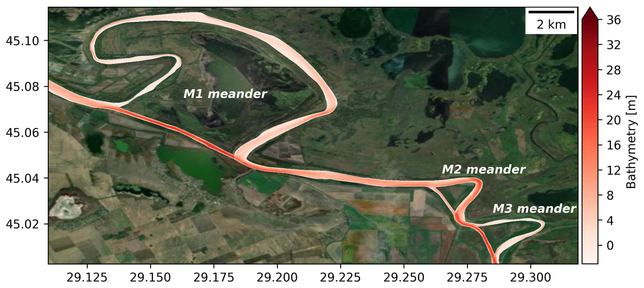
Figure 5 Map of the interpolated bathymetry in a section of the Sfantu Gheorghe branch. The M1 and M3 meanders present a shallower bathymetry than their respective artificial canals, while the M2 meander is deeper than its artificial cut-off channel. The background image is the Esri World Imagery basemap (ESRI, 2025).

Not all of the Sfantu Gheorghe branch meanders exhibit the same behaviours (Fig. 5). For example, while the M1 and M3 meanders are indeed shallower than their respective artificial canals, the M2 meander displays the opposite pattern. Tiron Duţu et al. (2014) observed the same phenomenon, attributing it to the fact that the M2 meander has retained much of its activity, with its artificial canal being comparatively less active than those associated with M1 and M3. This unequal distribution of flow between the meander and the artificial canal is attributed to several geomorphological control factors, including the channel length ratios, the diversion angle (i.e. the angle between the main channel and the entrance of the diversion channel), and the bed level differences.

4 Validation, applications, and limitations

4.1 Validation

The RRMSE for each segment is strongly influenced by the primary bathymetric source (Fig. 6). Segments predominantly based on UkrSCES data show an average RRMSE of 27.6±13.4 % (RMSE = 1.78 m). In contrast, segments primarily using AFDJ data exhibit a lower average RRMSE of 0.55±0.34 % (RMSE = 0.07 m). In segments where DDNIRD serves as the primary data source, the average RRMSE is 6.3±2.55 % (RMSE = 0.5 m). In the connection zones, where a weighted mean was calculated to ensure smooth transitions between segments, the average RRMSE is 1.90 % (RMSE = 0.26 m).

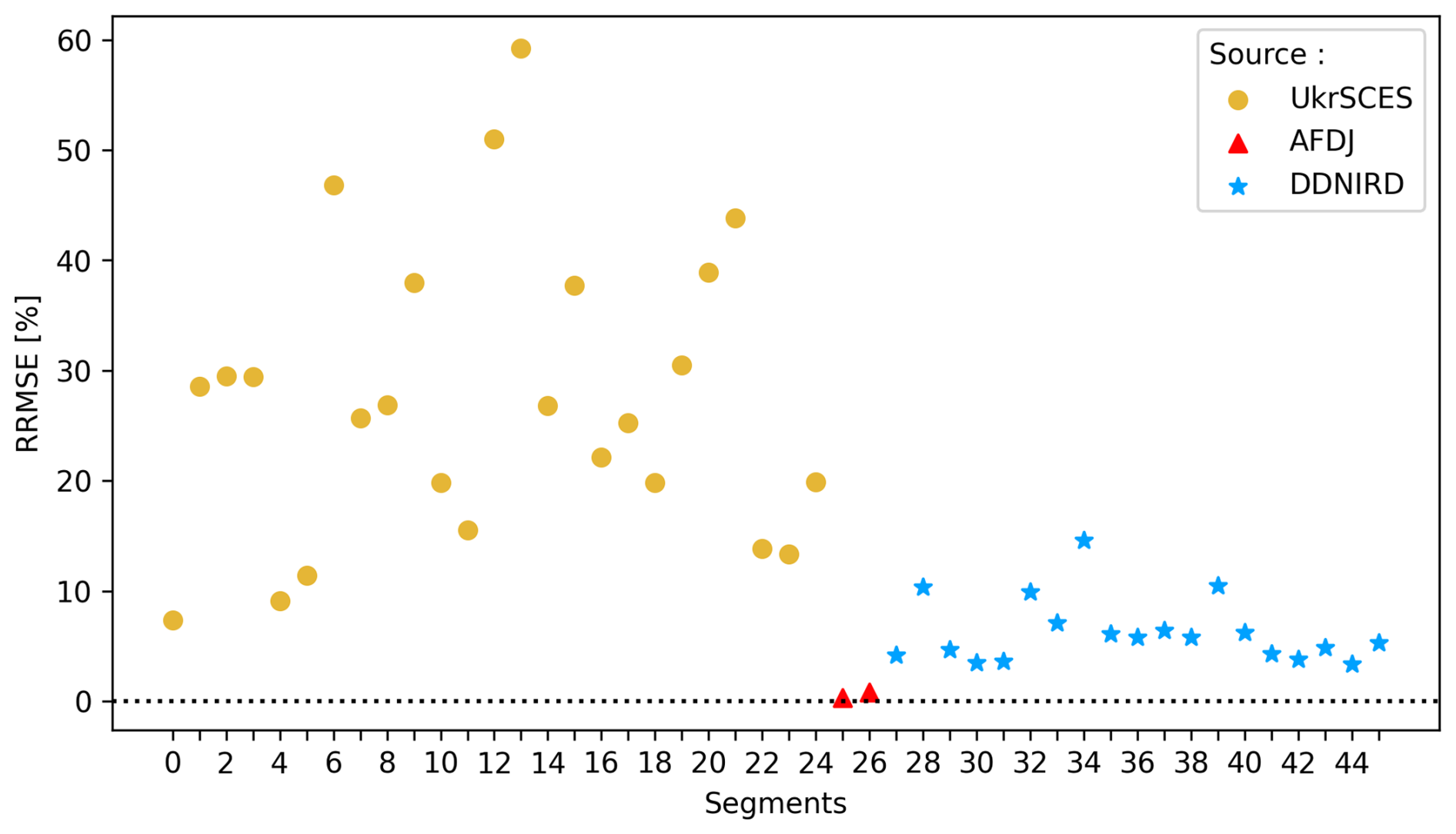
Figure 6 RRMSE for the bathymetry of each segment. The colours and shapes of the markers correspond to the main bathymetric data source covering the segment. The horizontal dotted line highlights the 0 % RRMSE line.

These results are comparable to those reported in studies using similar interpolation techniques. We did not find any studies that used datasets with a point resolution as low as that of the UkrSCES dataset. However, the RRMSE obtained for UkrSCES covered segments similar to those of Merwade (2009) for two rivers with a random point distribution and a density approximately 3000 times higher than the UkrSCES dataset. For the DDNIRD dataset, our results are on par with or better than those found in the literature with transect and similar point densities (Merwade, 2009; Liang et al., 2022). We also found no studies using datasets with a point density as high as that of AFDJ, but our RRMSE in AFDJ-dominated segments is close to 0, indicating excellent alignment with the observed data. Additionally, our results conform to well-established river morphological patterns. They present a greater variation in depth across the river than along its flow and deeper areas on the outer bends. The bathymetry in the Sfantu Gheorghe meanders reflects what was observed by Tiron Duţu et al. (2014). As a result, we consider the bathymetric product to be of the highest possible quality with the available data sources.

4.2 Comparison with global bathymetry models

Our bathymetry product presents a significant improvement in representing the Danube Delta over global bathymetry models like ETOPO 2022 and GEBCO 2024 (Fig. 7). With a grid resolution of ∼330 m, these global models struggle to represent the river bathymetry. In many cases, they either fail to capture the river's course or significantly underestimate its depth. Due to the coarse pixel size, which frequently exceeds the width of the river, they are unable to represent the depth variations within the river channel. While ETOPO 2022 and GEBCO 2024 are good bathymetry products for oceanographic applications, they lack the necessary resolution to represent river processes. In contrast, our bathymetry product, which has a much higher resolution, is specifically tailored to capture these critical riverine dynamics, making it a more suitable tool for river-related studies and models.

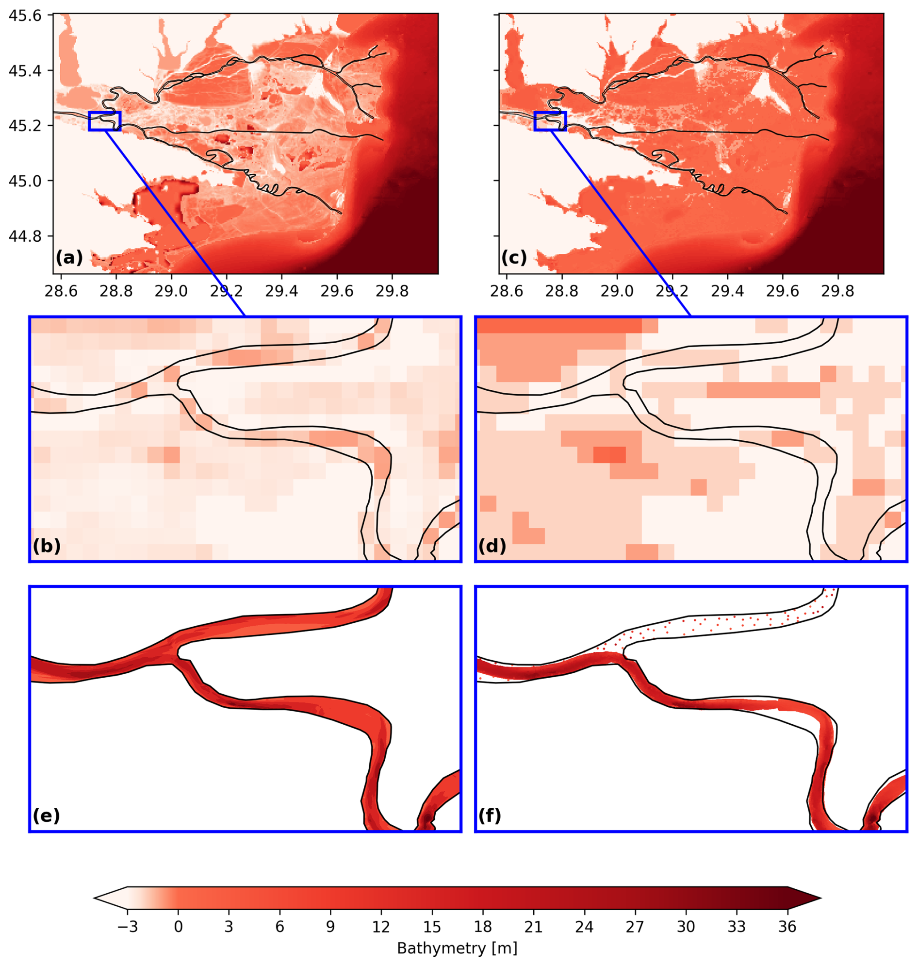
Figure 7 Comparison of the ETOPO 2022 and GEBCO 2024 bathymetry of the delta with this study's results and observations. The black line represents the Danube's riverbanks. (a) Delta bathymetry according to ETOPO 2022 (NOAA National Centers for Environmental Information, 2022), with (b) a close-up view of the ETOPO 2022 data on the Danube. (c) Delta bathymetry according to GEBCO 2024 (GEBCO Bathymetric Compilation Group, 2024), with (d) a close-up view of the GEBCO 2024 data on the Danube. (e) The bathymetry product presented in this study. (f) The observation data points used in this study.

4.3 Limitations

The most obvious limitation of this study comes from the data used. The first problem is linked to the data resolution. In particular, additional bathymetric data would be beneficial for river segments covered by the UkrSCES and DDNIRD datasets, and a higher-resolution DEM could improve shoreline delineation. For the UkrSCES dataset, the overall number of points is too low, and more data points should be taken, with special care to take points all across the width of the river. In the case of DDNIRD, the overall density is good, but the spacing between the transects is too high to ensure correct representation of the continuity of the bed between measurements. To improve the quality of the results, the best solution would be to increase the density of points in the river, particularly for the UkrSCES dataset and, to a lesser extent, the DDNIRD dataset. For the former, any input of bathymetry points would be useful, as random-based bathymetry datasets can achieve performances comparable to transect-based data if the density is high enough and points are correctly distributed across the width of the river (Merwade, 2009). For segments covered by the DDNIRD dataset, we suggest increasing the transect frequency or adding longitudinal profiles parallel to the shores, as proposed by Diaconu et al. (2019). Concerning the topography data, the 30 m resolution of the Copernicus DEM may be insufficient to precisely define the riverbank positions. A higher-resolution DEM could improve accuracy, but to our knowledge no such dataset is publicly available for this region.

The other limitation linked to the data stems from the temporal disparity between the datasets. The different measurements used in this study were taken between 2024 and 2021. The AFDJ and DDNIRD datasets were each collected within a single year, in 2018 and 2015, respectively. This is not the case for the UkrSCES dataset, whose data span 4 years (2014–2017). The topography readings originate from the 2021 Copernicus DEM. Rivers are very dynamic ecosystems, and the Danube is no exception, with both natural erosion and deposition of sediments and artificial dredging happening at different points along the river (Jugaru Tiron et al., 2009; Habersack et al., 2016; FAIRway Danube, 2021). It is therefore highly unlikely that the bathymetry and position of the riverbanks remained the same during the entire sampling period. As such, it is only natural that we observed discrepancies at places where two different bathymetry sources meet. Despite this, the datasets used in this study were carefully selected to minimize temporal gaps while prioritizing the highest available spatial resolution and accessibility, ensuring the best possible representation of the riverbed for an easy-access bathymetry product. Regarding the Copernicus DEM, since no product was available for the years corresponding to the bathymetry measurements, we used the latest available dataset at the time of data collection, as it provided the best possible topographic coverage for the region.

The by-segment interpolation used to allow re-projection in the s–n coordinate system is also a source of discontinuity between the segments. The use of a weighted mean combination method in the connection zones reduced those discontinuities in the interpolation results and allowed for more realistic transitions.

4.4 Applications

This work presents the first bathymetry dataset that comprehensively covers all three branches of the Danube Delta, marking a significant advance in the characterization and understanding of the delta.

One of the possible applications of this dataset is its use in a hydro-biogeochemical model of the Danube–Black Sea continuum. The Danube Delta plays an important buffering role between the river and the sea, but most present-day models do not represent the delta (Grégoire and Friedrich, 2004; Beckers et al., 2002; Kara et al., 2008; Kubryakov et al., 2018; Lima et al., 2020). This oversimplification can lead to inaccuracies in the representation of riverine inputs into the sea, which can in turn significantly impact the simulation of coastal processes (Ivanov et al., 2020; Breitburg et al., 2018; Bonamano et al., 2024; Rose et al., 2017). Therefore, having a high-resolution, easily accessible bathymetry dataset for the Danube Delta's branches is an important step towards improving the Black Sea coastal models and better understanding interactions within the Danube–Black Sea continuum. With that application in mind, future improvements to this dataset could include extending coverage to the shallow coastal waters in front of the delta.

Our bathymetry product could also be useful for flood risk assessment in the Danube Delta. The region is characterized by low elevations and minor altitude variations, with ∼93 % of its surface lying between 0 and 2 m above sea level. As a result, and despite the moderate rainfall in that area, the Danube Delta experiences annual flooding (Niculescu et al., 2015). Coupled with a high-precision DEM, our bathymetry dataset could be used to represent the flooding processes within the delta. It could also support evaluations of infrastructure impacts, such as those of dikes and floodplain modifications, on flood extent and dynamics.

In addition, this bathymetry dataset can be used in ecosystem and habitat modelling. Designated a UNESCO World Heritage Site since 1990, the Danube Delta is Europe's largest nearly undisturbed wetland and is considered a major biodiversity hotspot (Simon and Andrei, 2023; Sommerwerk et al., 2023). Water depth and, by extension, underwater topography are key components of habitat suitability models. They influence many wildlife activities, including fish breeding, benthic community distribution, reed bed development, and bird nesting (Zhang et al., 2024; Zigler et al., 2008; Sultanov, 2019). High-resolution bathymetry can help pinpoint areas of ecological importance and guide conservation efforts.

While this dataset is currently only available through conventional repositories, future developments could focus on integrating it into an interactive WebGIS platform. WebGIS tools are increasingly being used for disseminating scientific datasets in various fields (Dragićević, 2004; Pasquaré Mariotto et al., 2021; Foglini et al., 2025). They allow for easy access and wider dissemination of the information, providing broader accessibility beyond the scientific community, which typically engages with data repositories. Web-based platforms enable intuitive visualization, exploration, and interaction with the data, often incorporating tools for processing, analysis, and modelling. Although implementing such a system would require additional technical development and goes beyond the scope of this study, this could be a logical step towards enhancing the usability and impact of this dataset for a wider range of users, including policymakers, environmental managers, and researchers.

5 Data availability

The dataset generated from this work is available at https://doi.org/10.5281/zenodo.14055741 (Alaerts et al., 2024).

6 Conclusions

This dataset is the first unique, high-resolution, comprehensive, and easily accessible bathymetric model covering all three branches of the Danube Delta. We combined four different datasets of varying density and spatial patterns on a hybrid curvilinear–unstructured mesh using an anisotropic IDW interpolation method. The resulting product is made up of 5.8×10⁵ elements, with a resolution ranging from 2 to 100 m. Cross-validation confirmed that the error rates are comparable to those reported in similar interpolation studies, leading us to conclude that this product is as accurate as possible given the available data. By offering better resolution and accuracy, this product will allow more precise simulations of river–coastal dynamics, providing essential insights for both scientific research and environmental management in the region.

Appendix A: Mesh generation

To incorporate bathymetric data into hydrodynamic models, the river profile must be reconstructed on a mesh, ideally oriented in the flow direction (Merwade et al., 2005). In this study, we used a hybrid curvilinear–unstructured grid. It combines a curvilinear mesh made of quadrilateral elements elongated along the flow in unidirectional river segments and an unstructured triangular mesh at the connections between the segments (Fig. A1d). This hybrid curvilinear–unstructured grid has several advantages, the main one being that it allows accurate representation of the river bottom with limited data storage (Lai, 2010; Bomers et al., 2019).

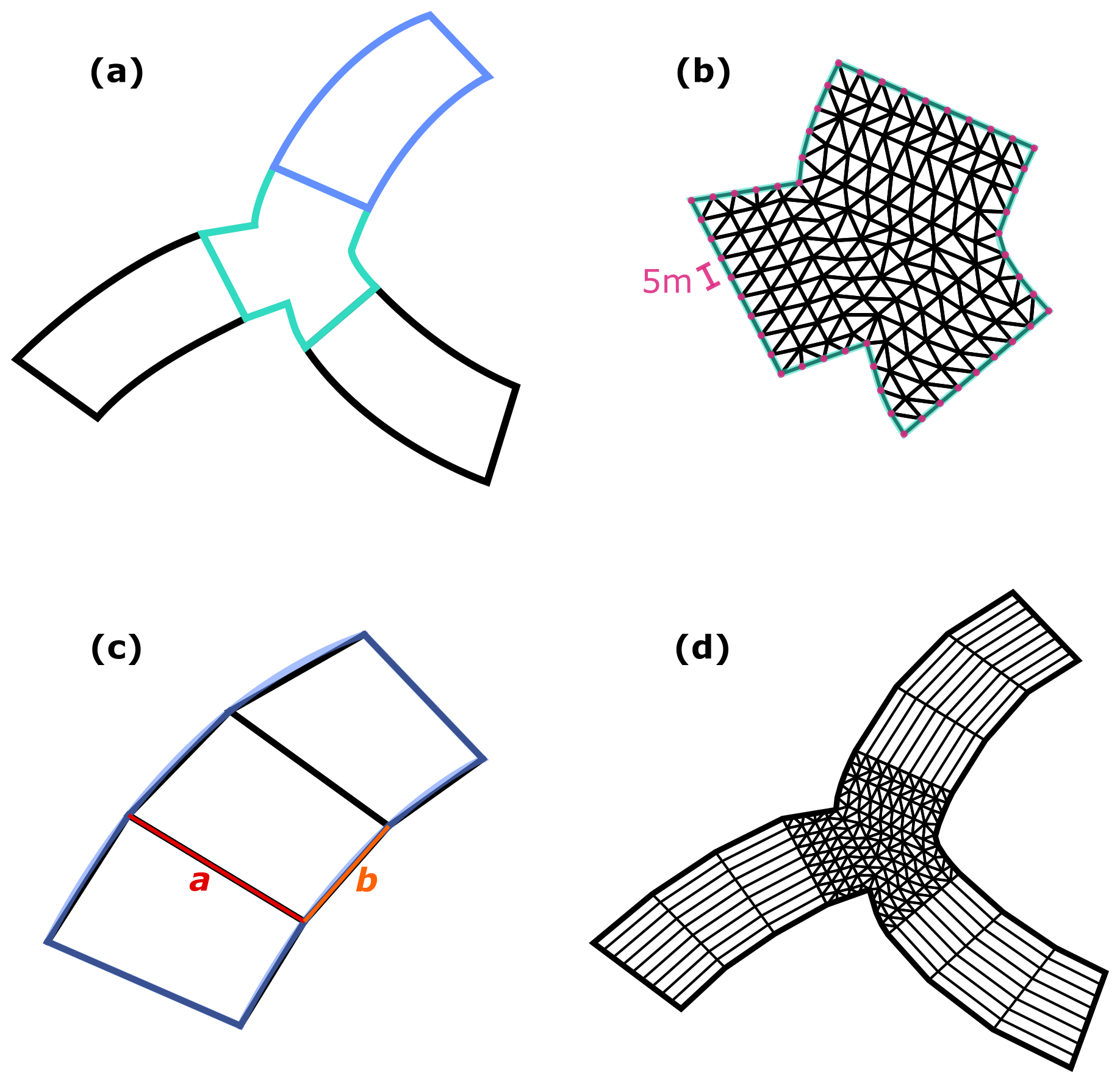
Figure A1 Creation of the mesh in the river. (a) The braided river is divided into unidirectional segments (black and blue) and connection zones (turquoise). (b) Connection zones are meshed with triangular elements at a resolution of approximately 5 m. (c) Segments are divided into quadrilaterals, where parameters a and b are optimized across each segment to ensure that the b edges are as close to a chosen length as possible and that a and b remain as perpendicular as possible (Eq. A1). (d) Segments are reassembled with connection zones. In each segment, each quadrilateral is further subdivided into smaller quadrilaterals aligned with the river's course in order to match the triangular elements of the connection zones.

To create the mesh, the Danube is first divided into unidirectional segments and connection zones (i.e. zones where the river segments split or merge) (Fig. A1a). To do so, the river is cut at a distance of L m from the points where the river segments intersect. We hence obtain 45 individual segments and 35 connection zones that will be meshed separately before being put back together. The connection zones are meshed using triangular elements with a resolution of l m (Fig. A1b). Each segment is then subdivided further into quadrilaterals by cutting both riverbanks at L m intervals. To optimize this division of the segments, we calculate the following metric for each quadrilateral:

$$\begin{array}{}\text{(A1)}& Q=\mathrm{10}\left(\right|\mathit{b}|L{)}^{\mathrm{4}}+(\mathit{b}\cdot \widehat{\mathit{a}}{)}^{\mathrm{4}},\end{array}$$

where b is a vector following the quadrilateral edge along the riverbank, L is the target length of b, and a is a vector following the edge of the same quadrilateral that serves as a cross section of the river (Fig. A1c). The quality metric Q is computed for each combination of a and b, and the sum of Q is minimized for each segment. The aim of this optimization is to have quadrilaterals with b as close as possible to the desired length L and where the angle between a and b is as close as possible to 90°. In this way, we avoid having elements that are too small in curved river segments or near connections. The segments are then assembled back together with the connection zones, and quadrilaterals in the segments are subdivided further into smaller ones to ensure alignment with the 5 m elements in the connection zones (Fig. A1d). The mesh was created using GMSH (https://gmsh.info/, last access: 18 March 2025) (Geuzaine and Remacle, 2009).

Our observation datasets have a resolution varying between a few metres and hundreds of metres. As a compromise, we chose to fix L=50 m and l=5 m, obtaining a mesh made of 5×50 m elements in the segments and 5 m elements in the connection zones. This resolution is consistent with the resolutions of recent hydrodynamic models in rivers and deltas that generally have minimum element sizes varying between 5 and 50 m (Pham Van et al., 2016; Pelckmans et al., 2021; Bunya et al., 2010; Dresback et al., 2023; Bakhtyar et al., 2020). While this resolution may be coarser than the original bathymetric data in certain areas, particularly those covered by the AFDJ dataset, it provides a unified dataset with sufficient details to use in advanced hydrodynamic models while being more manageable than non-integrated higher-resolution datasets.

Appendix B: Interpolation

B1 Interpolation process

Given the diverse data sources, a certain degree of standardization was necessary. First, we had to transition most of the data from their local datum to the WGS84 vertical datum. The UkrSCES data were referenced to the Odessa datum, which is 0.17 m below the WGS84 vertical datum. For the AFDJ data, most of the Sulina channel was referenced to the Marea Neagra Sulina datum, 0.03 m above WGS84, while data upstream of Tulcea and the beginning of the Sulina channel used the Tulcea datum, 0.33 m above WGS84. The DDNIRD data were referenced to the Marea Neagra 75 datum, 0.25 m above WGS84 (Anastasiu, 2014).

Next, we interpolated the data onto the mesh. A first common step in river interpolation is to project the bathymetric data onto a segment-oriented s–n coordinate system (Merwade et al., 2005, 2006; Pelckmans et al., 2021; Legleiter and Kyriakidis, 2008). This projection improves interpolation results, as conventional Cartesian interpolation methods often struggle to capture riverbed topography accurately because of the strong anisotropy of river systems. Depth variations are typically much more pronounced across the river (perpendicular to the flow) than along its course. The initial projection of bathymetric data onto an s–n coordinate system allows us to account for this anisotropy in the following interpolation. In this study, s represents the distance along the centre line of the river, while n is the distance on the perpendicular to s.

Each river segment, as defined during mesh generation, has its own s–n coordinate system. The projection process inside a segment is described below and illustrated in Fig. B1:

1. Definition of the s–n coordinate system. The river centre line is computed as the middle point between each pair of opposing bank nodes (Fig. B1a). This centre line serves as the s axis. The s coordinate of each pair of opposing bank nodes is determined by measuring the centre line distance from the segment's starting point to the line connecting the two nodes (Fig. B1b). The n coordinate is assigned to each node on the banks by halving the distance between the opposing nodes (Fig. B1c). Nodes on the right bank have a negative n coordinate, and nodes on the left bank have a positive coordinate. This results in a grid of quadrilateral elements, where each corner node has a new coordinate within the s–n system of the segment.

2. Re-projection of the bathymetry points. Each bathymetry point is assigned to the quadrilateral it falls within (Fig. B1d). The s–n coordinates of the bathymetry point are calculated (Fig. B1e) with

   $$\begin{array}{}\text{(B1)}& \begin{array}{rl}& s={\displaystyle \frac{\mathrm{1}-{\mathit{\delta }}_x}{\mathrm{2}}}{s}_{x_{\mathrm{0}}}+{\displaystyle \frac{\mathrm{1}+{\mathit{\delta }}_x}{\mathrm{2}}}{s}_{x_{\mathrm{1}}},\\ & n=\left({\displaystyle \frac{\mathrm{1}-{\mathit{\delta }}_x}{\mathrm{2}}}{n}_{x_{\mathrm{0}}}+{\displaystyle \frac{\mathrm{1}+{\mathit{\delta }}_x}{\mathrm{2}}}{n}_{x_{\mathrm{1}}}\right){\displaystyle \frac{\mathrm{1}-{\mathit{\delta }}_y}{\mathrm{2}}}\\ & +\left({\displaystyle \frac{\mathrm{1}-{\mathit{\delta }}_x}{\mathrm{2}}}{n}_{x_{\mathrm{3}}}+{\displaystyle \frac{\mathrm{1}+{\mathit{\delta }}_x}{\mathrm{2}}}{n}_{x_{\mathrm{2}}}\right){\displaystyle \frac{\mathrm{1}+{\mathit{\delta }}_y}{\mathrm{2}}},\end{array}\end{array}$$

   where δ_x and δ_y are the point's local coordinates within the quadrilateral and $s_{x_i}$ and $n_{x_i}$ are the s–n coordinates of the ith corner node of the quadrilateral.

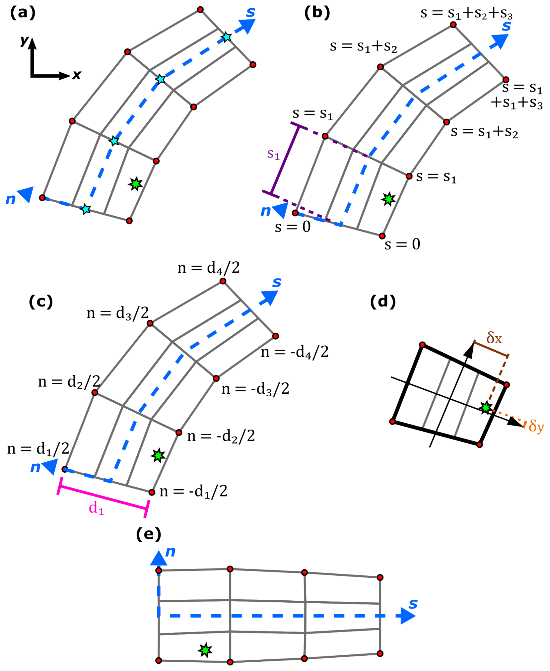
Figure B1 Re-projection of the bathymetry points onto the s–n coordinate system. The bathymetry point is represented by a green star. The nodes on the riverbanks are represented by the red circles. The mesh is represented by the grey lines. (a) We find the centre line (blue dotted line) of the river segment. The centre line passes through the middle (blue stars) of every pair of opposing nodes. (b) Every node on the riverbanks receives an s coordinate. (c) Every node on the riverbanks receives an n coordinate. (d) Coordinates of the bathymetry points in the quadrilateral in which they are located. (e) Bathymetry point in the s–n coordinate system.

To account for the river anisotropy during interpolation in the segments, one approach is to give more weight to points with similar n coordinates (i.e. directly upstream or downstream) than those with similar s coordinates (i.e. on the same transect) (Merwade et al., 2006, 2008; Wu et al., 2019). To achieve this, we multiplied the n coordinate of every point by a dimensionless anisotropy factor an to artificially increase the distance between bathymetry points in the direction perpendicular to the river. Bathymetry values at mesh nodes were then computed using IDW interpolation:

$$\begin{array}{}\text{(B2)}& z^{*}=\sum _{i=\mathrm{1}}^{np}{w}_i{z}_i,\end{array}$$

where z^* is the interpolated depth, i=1, … np are the np bathymetry points closest to the node, z_i is the depth of the ith bathymetry point, and w_i is the weight associated with this point:

$$\begin{array}{}\text{(B3)}& w_i={\displaystyle \frac{\frac{\mathrm{1}}{d_i^p}}{\sum _{i=\mathrm{1}}^{np}\frac{\mathrm{1}}{d_i^p}}},\end{array}$$

where d_i is the distance between the node and the ith bathymetry point and p is an exponent controlling the influence that the points have on the interpolation. A higher p value reduces the effect of distant points on the interpolation. Similar methods, where the IDW interpolation is modified to take into account the anisotropy of the river, have given good results in previous studies, even outperforming other interpolation methods such as kriging or spline interpolation (Merwade et al., 2006; Liang et al., 2022; Diaconu et al., 2019).

Another challenge in this study was handling interpolation in the connection zones, where multiple river segments converge or diverge. In these areas, the deepest parts of the river do not follow a single, easily defined direction that can be approximated by a centre line s. Instead, bathymetric features form complex patterns, often extending from adjacent segments and intersecting in “T” or “X” configurations. Few studies on river bathymetry interpolation focus on braided rivers with multiple river segments. Goff and Nordfjord (2004) included the connection zones within the river segments and took the maximum interpolated depth at points with multiple interpolation results. Hilton et al. (2019) employed an s–n coordinate system that covered the entire braided river network, with the n coordinate spanning from 1 at the northernmost riverbank to −1 at the southernmost riverbank, thus avoiding the need to divide the network into separate segments. Similarly, Lai et al. (2021) kept the whole river network and linearly interpolated the bathymetry along the streamlines. In contrast, Dey et al. (2022) segmented the network and interpolated points in the connection zones using a two- or three-neighbour IDW approach, depending on whether the points were on the tributary side of the thalweg. While these methods produce satisfactory results, they also present limitations in terms of complexity or compatibility with our domain. In this study, we chose to elongate the segment's mesh in order to create a grid that extends into the surrounding connection zones. This grid then served as a reference grid for projecting both the mesh points and bathymetric data within the connection areas, following the procedure illustrated in Fig. B1. Interpolation was then performed as if the mesh points of the connection zones included in this extended grid belonged to the segment. As a result, each point in a connection zone could be assigned multiple bathymetry values from the interpolation in the different neighbouring segments. To determine the final bathymetry value for these points, we tested three different combination methods. The first method followed the Goff and Nordfjord (2004) approach, selecting the maximum value among the results. In the second method, we calculated the mean of the values. In the third method, we averaged the interpolation results with weights inversely proportional to the distance from the segment generating each result. These three methods are hereafter referred to as the max, mean, and weighted mean methods, respectively.

B2 Parameterization

A sensitivity analysis was carried out to identify the optimal values for the parameters an, np, and p of the interpolation method (Eqs. B2 and B3) in the river segments. For the anisotropy factor an, we tested integers between 1 and 20, followed by multiples of 10 up to 100. The maximum value of 100 was chosen based on the DDNIRD data, where the distance within a transect is approximately 3 m, while the distance between transects is about 300 m. The values tested for the number of neighbours np and the exponent p are, respectively, integers between 2 and 8 and integers between 1 and 3. To select the best set of parameters, we looked for the set of parameters that minimized the error obtained with the leave-one-out cross-validation technique. For segments with more than 1000 points, where a random sample of 1000 points was used for testing, the same 1000 points were tested for each parameter set.

The optimal parameters for each segment are presented in Tables B1 and B2. Overall, we did not find any definitive rule to define the optimal values of the an, np, and p parameters of the segments. However, certain trends can be observed regarding the dimensionless anisotropic factor an. Segments covered by bathymetry primarily sourced from UkrSCES data tend to require a higher an value, with a median of 18. Segments relying on AFDJ or DDNIRD data have lower median an values of 1 and 2, respectively. We observed no clear trend between the optimal values of the other parameters and the source of the observation data. Segments mainly relying on AFDJ data appear to be insensitive to variations in parameter values.

Table B1 Combination of parameters for the interpolation of the bathymetry that gives the lowest error for each segment covered by the UkrSCES dataset.

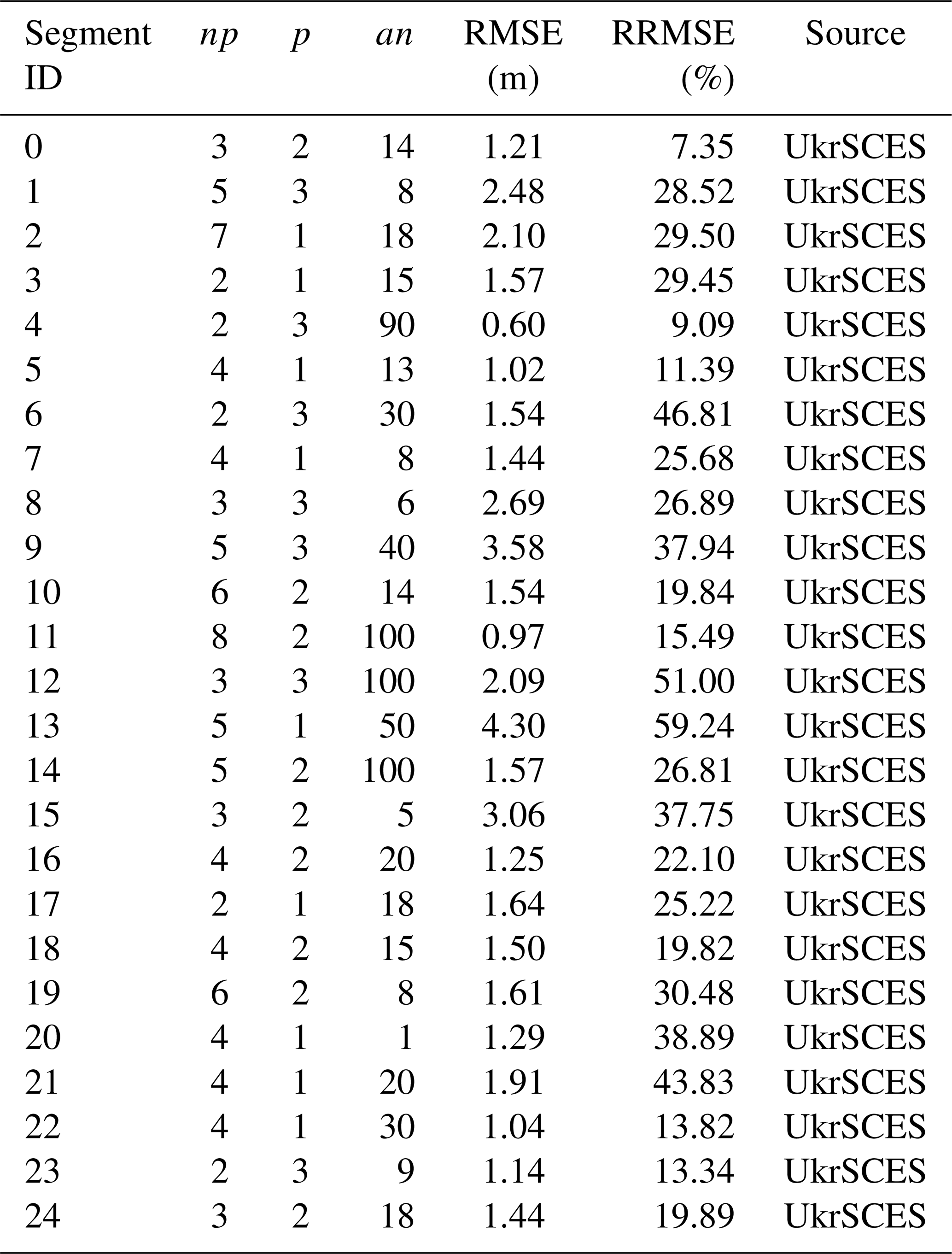
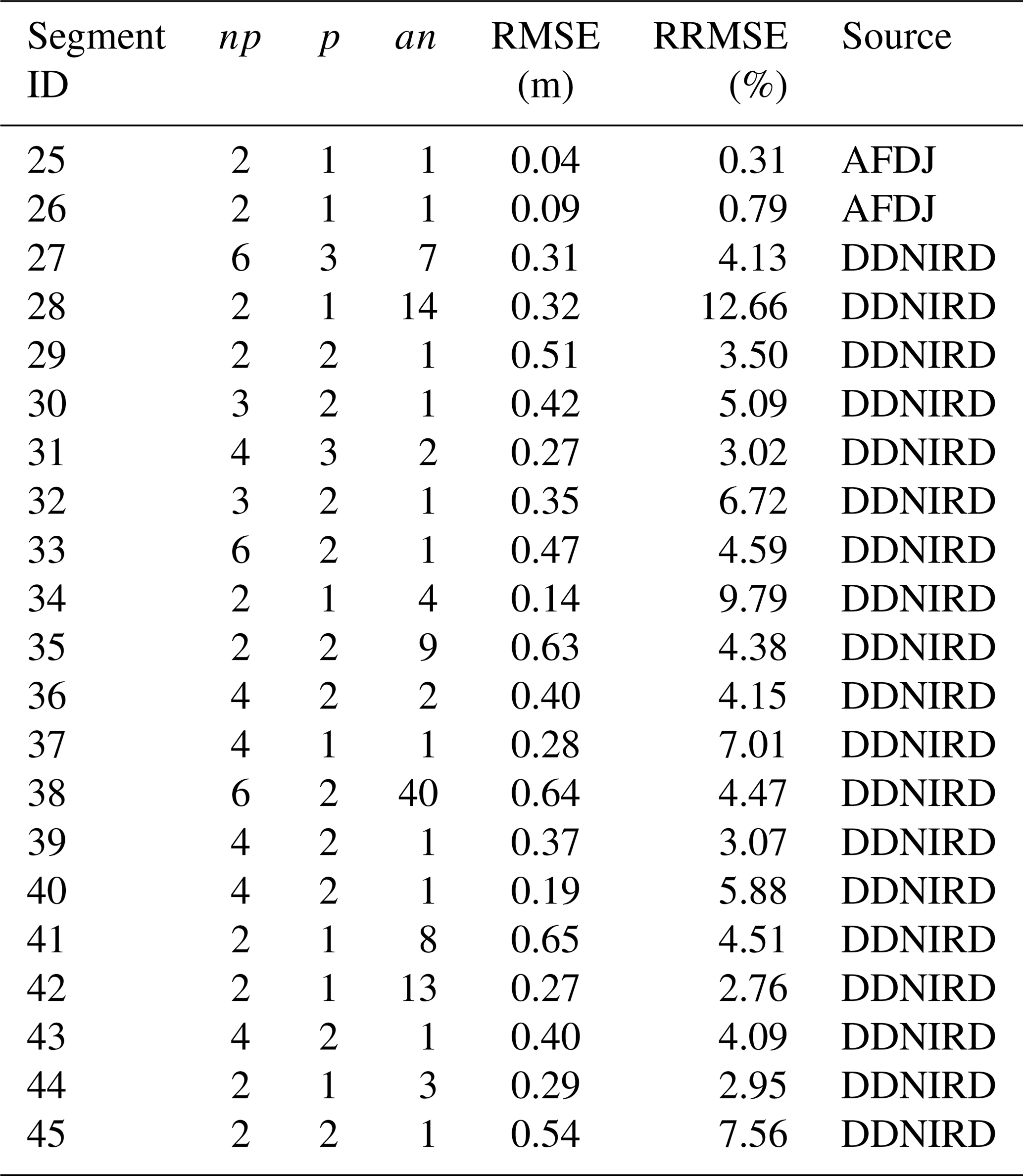
Table B2 Combination of parameters for the interpolation of the bathymetry that gives the lowest error for each segment covered by the AFDJ or DDNIRD datasets.

This initial parameterization worked well for sparse, randomly distributed bathymetric data and high-density bathymetry, such as the data from the UkrSCES and AFDJ. For the DDNIRD data, where points within transects are densely packed and transects are widely spaced, this method led to interpolation errors on the higher-resolution grid. When optimizing parameters in segments with DDNIRD data by sequentially removing points, the optimal an value was often low. This is due to the fact that points within the same transect are very close to each other and have similar bathymetry values, unlike the more distant points in other transects. As a result, when the mesh resolution along the s axis is finer than the distance between transects, the np bathymetric points closest to the mesh nodes are often all from the same transect. This created a step-like interpolation, disrupting along-bed continuity.

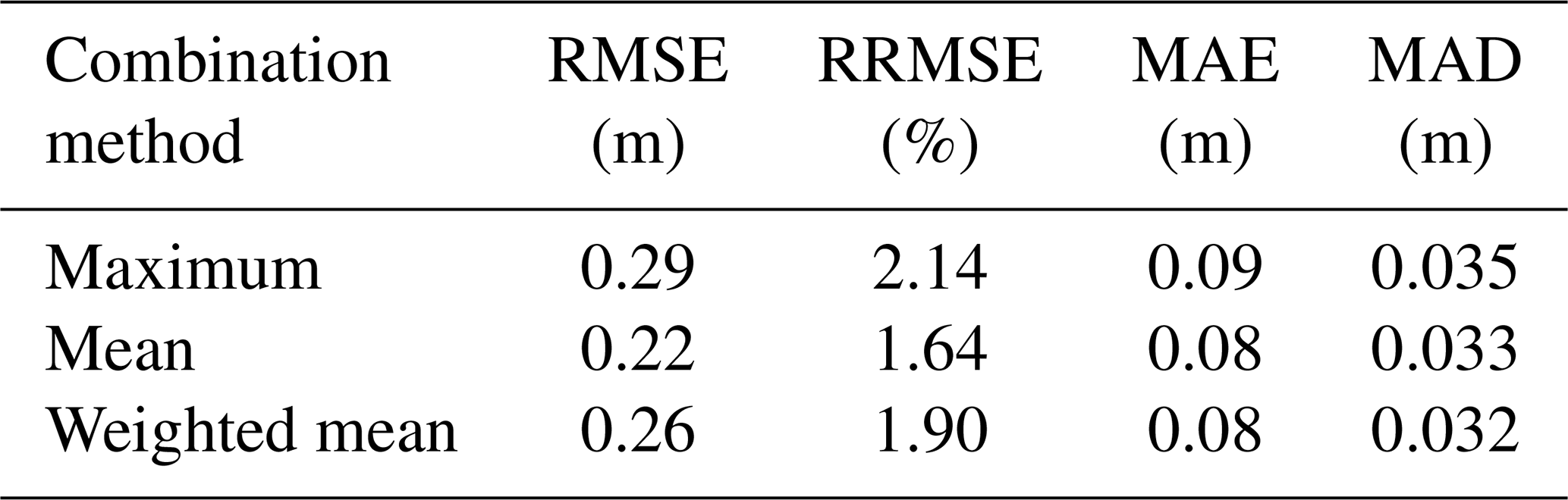
Table B3 Error metrics in connection zones corresponding to the different combination methods described in Sect. B.

To address this issue, we employed a modified two-step interpolation technique within the s–n coordinate system for segments where DDNIRD data predominate. The first step is based on the idea pursued by several studies that the bathymetry changes linearly following lines of constant n coordinates (Goff and Nordfjord, 2004; Caviedes-Voullième et al., 2014; Dysarz, 2018). For each grid point of the grid used for reprojection, we computed the bathymetry by identifying the points closest to the upstream and downstream transects and then applying a simple IDW interpolation using those two points in Eqs. (B2) and (B3), with np=2 and p=1. This process results in bathymetric data whose coordinates align with the mesh within the segment but not in the connection zones. To resolve this, a second interpolation is performed using the same method as with other bathymetry sources but with the grid-interpolated bathymetry as the source. Since the grid and mesh coincide within the segments, the interpolated bathymetry in these areas remains largely unaffected by the second step, while the bathymetry on the mesh points in the connections continues smoothly from the segments. To estimate the error with this method, we used a leave-one-out cross-validation technique to compute the RRMSE on the observation points. It is important to note that this approach does not provide an error estimation for the mesh nodes between the transects.

In the connection zones, the three tested combination methods have similar errors (Table B3). They all gave low error metrics, with at least 50 % of the tested points having an absolute error below 3.5 cm. The max method gives the poorest results. Although the mean method resulted in the lowest overall error, the weighted mean method provided smoother transitions between the segments and has a lower median absolute deviation (MAD).