Tracer-based Rapid Anthropogenic Carbon Estimation (TRACE)

The ocean is one of the largest sinks for anthropogenic carbon dioxide (C_anth) and its removal of carbon dioxide (CO₂) from the atmosphere has been valued at hundreds of billions to trillions of US dollars in climate mitigation annually. The ecosystem impacts caused by planet-wide shifts in ocean chemistry resulting from marine C_anth accumulation are an active area of research. For these reasons, we need accessible tools to quantify ocean C_anth inventories and distributions and to predict how they might evolve in response to future emissions and mitigation activities. Unfortunately, C_anth estimation methods are typically only accessible to trained scientists and modelers with access to significant computational resources. Here, we make modifications to the transit time distribution approach for C_anth estimation that render the method more accessible. We also release software (BRCScienceProducts, 2025) called “Tracer-based Rapid Anthropogenic Carbon Estimation version 1” (TRACEv1) that allows users – with one line of code – to obtain C_anth and water mass age estimates throughout the global open ocean from user-supplied values of geographic location, pressure, salinity, temperature, and the estimate year. We use this code to generate a data product of global gridded open-ocean C_anth distributions (TRACEv1_GGC_anth; Carter, 2025) that ranges from the preindustrial era through 2500 under a range of Shared Socioeconomic Pathways (SSPs, or atmospheric CO₂ concentration pathways). We estimated the skill of these estimates by reconstructing C_anth in models with known distributions of C_anth and transient tracers and by conducting perturbation tests. In the model-based reconstruction test, TRACEv1 reproduces the global ocean C_anth inventory to within ±10 % in 1980 and 2014. We discuss implications and limitations of the projected C_anth distributions and highlight ways that the estimation strategy might be improved. One finding is that the ocean will continue to increase its net C_anth inventory at least through 2500 due to deep-ocean ventilation, even with the SSP in which intense mitigation successfully decreases atmospheric C_anth by ∼60 % in 2500 relative to the 2024 concentration. A notable limitation of this and similar projections made with TRACEv1 is that ongoing and potential future warming and changing oceanic circulation patterns with climate change are not captured by the method. The data products generated by this research are available as MATLAB code (https://doi.org/10.5281/zenodo.15692788, BRCScienceProducts, 2025) and a spatially and temporally gridded data product (https://doi.org/10.5281/zenodo.15692788, BRCScienceProducts, 2025).

1 Introduction

Humans are emitting ∼10 PgC as carbon dioxide gas (CO₂) to the atmosphere every year, and a portion of these emissions (∼25 %) has entered the ocean (Friedlingstein et al., 2022). Ocean carbon accumulation mitigates global warming by slowing atmospheric CO₂ accumulation. However – in a series of chemical processes known as ocean acidification – the elevated carbon content in seawater also shifts ocean carbonate chemistry toward a lower pH and carbonate ion content and toward a higher hydrogen ion (H⁺) content and CO₂ partial pressure (pCO₂). These chemical shifts have varying and important impacts on marine organisms and potentially on entire ocean ecosystems (Doney et al., 2009, 2020). It is important to be able to distinguish between the ocean's large natural background dissolved inorganic carbon (DIC) content and the excess anthropogenic carbon (C_anth) if we are to understand the extent, climate impact, and likely future outcomes of ocean C_anth accumulation.

Ocean C_anth is defined as the difference between the DIC in the modern ocean and the DIC that would be present if humans had never emitted CO₂ (Sabine et al., 2004). It is not a measurable quantity as defined. Without a direct measure, C_anth must be estimated, and there are numerous approaches to estimating C_anth within the literature, including the following: global ocean biogeochemical model (GOBM) simulations (Khatiwala et al., 2013), data-assimilation-based ocean circulation models coupled with air–sea exchange parameterizations (Devries, 2014), approaches that rely on preformed property estimates and remineralization ratios (Vázquez-Rodríguez et al., 2009) or empirical relationships (Touratier and Goyet, 2004; Yool et al., 2010), comparisons of repeated hydrographic sections (Carter et al., 2019; Gruber et al., 2019b; Müller et al., 2023), techniques such as the transit time distribution (TTD) or Green function approaches that rely on transient tracers of air–sea exchange to infer histories of atmospheric contact and interior ocean circulation (Khatiwala et al., 2009; Waugh et al., 2006), and approaches that combine one or more of these other approaches (Sabine et al., 2004). Isotopic approaches address the related, although not identical, question of “how much of the DIC in seawater is of anthropogenic origin (e.g., Eide et al., 2017)?”. Research continues to improve upon these methodologies and to better quantify their uncertainties, often using reconstructions of exactly known model-simulated C_anth distributions (Carter et al., 2019; Clement and Gruber, 2018; He et al., 2018; Matsumoto and Gruber, 2005; Waugh et al., 2006).

There are several qualities that are desirable for C_anth estimation strategies. Foremost among these is accuracy, but it is also helpful for estimation approaches to be (1) accessible, (2) computationally efficient, and (3) able to return estimates for the past, present, or future. The importance of these latter three qualities is outlined in the following:

1. Accessibility. Implementation of most C_anth estimation strategies requires nuanced understanding of the methodology so that decisions can be made about the parameters used in forward or inverse models or how and whether to account for various biogeochemical processes (e.g., calcification, organic matter ballasting, or iron dynamics and limitation). In addition, many C_anth estimation strategies require the presence of co-located high-quality measurements of physical and biogeochemical properties (e.g., empirical multiple linear regression C_anth change estimates) or transient tracer content measurements (e.g., TTD or Green-function-based estimates).

2. Computational efficiency. Some C_anth estimation strategies require downloading and employing large sparse matrices (Davila et al., 2022), whereas others require iterative inverse model reconstructions or forward model simulations to be run with GOBMs (DeVries et al., 2017; Khatiwala et al., 2013).

3. Able to be estimated for the past, present, or future. Many C_anth estimation techniques are limited to a narrow time window. For example, “extended multiple linear regression” approaches are usually limited to the period spanned by repeated shipboard hydrographic measurements (Carter et al., 2019; Gruber et al., 2019a; Müller et al., 2023). A related problem is the need to adjust a DIC dataset that was measured across years or decades to be specific to a single reference year or year of interest. To make this adjustment, it is important to know how much the DIC value would have changed due to C_anth accumulation between when it was measured and the reference year. Simplistic adjustments invoking transient steady-state (Gammon et al., 1982) C_anth accumulation are commonly employed (Carter et al., 2021a; Clement and Gruber, 2018; Lauvset et al., 2016; Müller et al., 2023), but they are problematic for larger adjustments that are often associated with longer time gaps. An example of an application that faces these challenges is given in Sect. S1 in the Supplement.

Here, we describe, assess, and present results from a new method that we call “Tracer-based Rapid Anthropogenic Carbon Estimation version 1”, or TRACEv1, which aims to provide C_anth estimation that meets these needs without overly compromising on C_anth estimate accuracy. TRACEv1 is an approach that retains much of the skill of the more complex approaches and yet is quick; nearly global; easy to use; computationally efficient; able to generate plausible projections over a limited time horizon; and requires only coordinate information (longitude, latitude, and depth), salinity (S), temperature (T), the desired year for the estimate, and (for projections) the assumed Shared Socioeconomic Pathway (i.e., SSP, or atmospheric CO₂ concentration over time).

In this paper, we present three products. The first is the TRACEv1 code itself; the code is initially released only for the MATLAB computing language, although a Python port is planned. The code contains subroutines that use neural networks to remap the preformed property estimates of Carter et al. (2021b) to the locations and conditions provided by users calling the TRACEv1 routine. The second is an estimate of the likely uncertainties in TRACEv1 estimates based on an analysis of the errors found when the method is trained using transient tracer information extracted from a GOBM simulation – with a spatial and temporal distribution that mirrors the availability of CFC-11, CFC-12, and SF₆ measurements in the real ocean – and is used to reconstruct the exactly known GOBM C_anth distributions. The third is a data product of global C_anth from TRACEv1 with varied 10- to 100-year resolution from 1750 through 2500. This product uses a variety of SSPs for projections after 2015.

2 Methods

First, we describe the conceptual framework for TRACEv1 and explain in detail how it works. Second, we introduce the observational datasets used to train TRACEv1 and explain how TTD parameters and preformed properties are empirically fit and estimated on demand. Finally, we explain how TRACEv1 is used to generate the TRACEv1_GGC_anth product (Carter, 2025).

2.1 Conceptual framework and historical context

TRACEv1 emulates the inverse Gaussian (IG) TTD method for C_anth estimation, although with several modifications. Traditionally, the TTD approach makes assumptions about the distribution of ages (length of time since seawater was last in contact with the atmospheric) of the various parcels of seawater that combine to produce the seawater observed in the ocean interior. Assumptions are also needed about the degree of air–sea equilibration with transient tracers. These assumptions are collectively used to tune the age distribution to match transient tracer observations, and similar assumptions are then used to infer the C_anth content that would be expected for that mixture of seawater from the distribution of ages and the known history of atmospheric CO₂ accumulation (e.g., He et al., 2018). TRACEv1 also follows these steps. The most important modification is that we reduce the TTD shape to a single term (α), optimize this term to reflect transient tracer and modeled ideal age distributions as normal, and then train a neural network capable of predicting this term using only physical measurements of seawater and coordinate information. This allows us to estimate C_anth from a TTD without the need for co-located transient tracer observations at the time and place where the estimate is desired.

When optimizing α, CFC-11, CFC-12, and SF₆ are dominant constraints for younger waters, while water mass ideal ages (A) (Thiele and Sarmiento, 1990) – taken from a model that assimilates transient tracer observations and measurements of the long-lived ¹⁴C radionuclide – are primarily included as a constraint for older water masses. SF₆ measurements are particularly strong constraints for the youngest waters ventilated since the 1990s maxima in CFC-11 and CFC-12 concentrations, but they are only available for ∼30 % of the measured bottles. All available constraints are used for optimizing all water parcels, and the strong constraint for young (old) waters and weak constraint for old (young) waters provided by transient tracers (A) is a natural result of how the values and misfits of each constraint vary with the age of the water mass. The transient tracer constraints therefore dominate in younger waters where the transient tracer measurements are largest, whereas the A constraint dominates in water masses that are older than the advent of measurable atmospheric transient tracer concentrations in the period from 1940 to the 1960s. For water parcels older than ∼1940, there is essentially no sensitivity to the transient tracer information. TRACEv1 is therefore more of an observation-based product in the surface ocean and an observation-tuned, model-based product in the deep ocean.

Several recent developments have enabled TRACEv1. First, the training data are taken from the recent 2023 update to the Global Data Analysis Project version 2 (GLODAPv2.2023) data product (Lauvset et al., 2024). This data product contains >270 000 bottle measurements with both CFC-11 and CFC-12 and >70 000 more measurements with CFCs and SF₆ measurements (Fig. 1); SF₆ was first included in the 2022 GLODAP release (Lauvset et al., 2022). CFC distributions have long been used to estimate C_anth, and oceanographic SF₆ measurements are available from many recent cruises owing to methodological developments by Tanhua et al. (2004) and advances allowing CFC and SF₆ measurements on the same samples (Bullister et al., 2006) implemented by transient tracer teams globally (Erickson et al., 2023). Second, water mass ideal ages from the recently released transport matrix solutions of the Ocean Circulation Inverse Model of John et al. (2020) provide an additional constraint for TRACEv1. TRACEv1 uses a preformed property data product (Carter et al., 2021b) to estimate the composition of seawater when it was last exchanging CO₂ with the atmosphere. Finally, the approach is assessed against newly simulated C_anth, CFC, and SF₆ distributions (Müller, 2023) that were generated as part of the second Regional Ocean Carbon Cycle Assessment and Processes effort (RECCAP2; e.g., DeVries et al., 2023). The simulated CFC and SF₆ distributions (Schwinger, 2024) were not previously published as part of the RECCAP2 data product or used by the analyses.

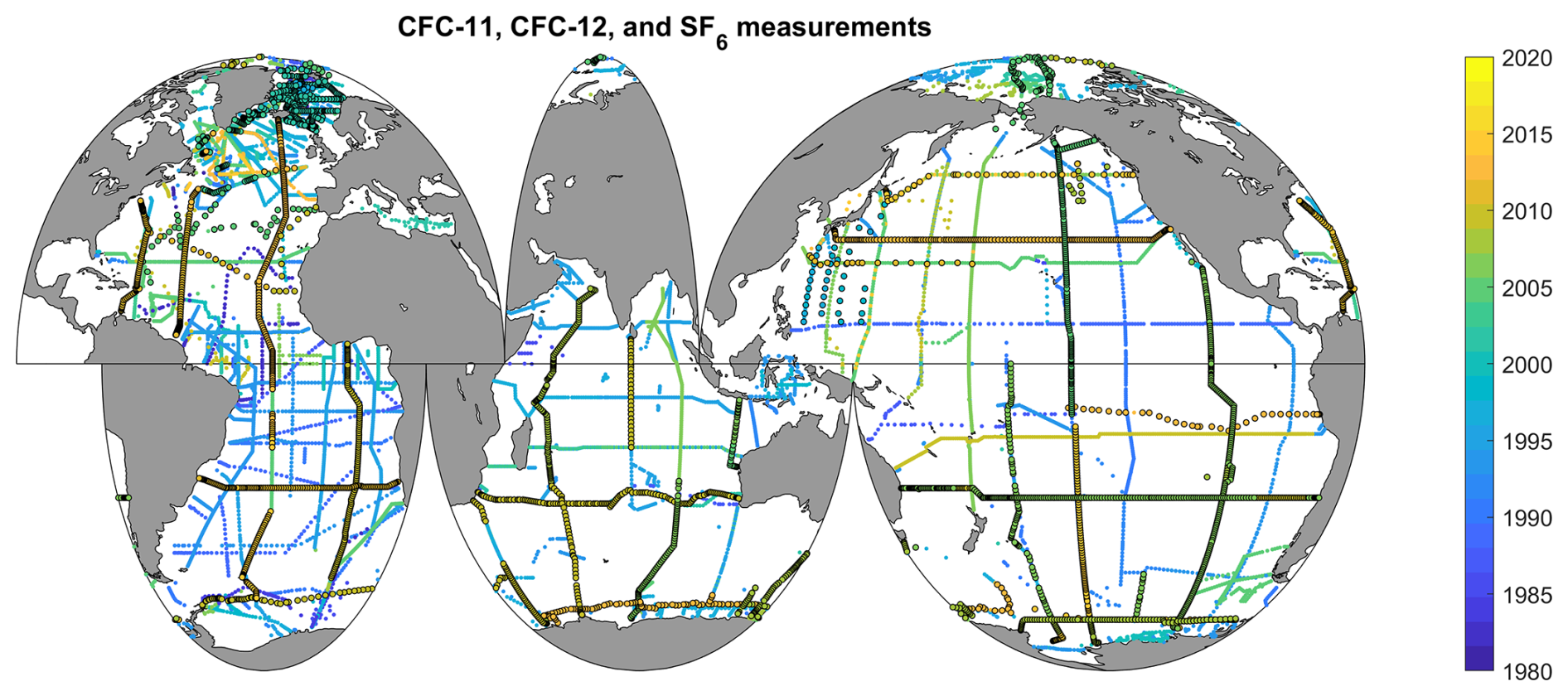
Figure 1 Locations and years of measurements of CFC-11 and CFC-12 in the GLODAPv2.2023 data product (Lauvset et al., 2024). Dark borders around measurements indicate that SF₆ is available alongside CFC-11 and CFC12.

2.2 How TRACEv1 works

We begin with a summary of the TRACEv1 functions and then explain the various steps in greater detail. The TRACEv1 code comprises the following functions:

1. It uses a neural network to estimate an age distribution for seawater from a user-specified location, T, and S, and it returns the mean age if this is a desired output.

2. TRACEv1 uses a record or projection of the atmospheric CO₂ in the years leading up to the date of the desired estimate to determine an anthropogenic CO₂ level for each component of the water mass mixture.

3. The code convolves the age distribution with the component's CO₂ history to estimate a component-fraction-weighted mean atmospheric CO₂ for the water parcel.

4. It uses another set of neural networks to estimate the preformed properties of this water mass mixture from the user-specified location, T, and S.

5. TRACEv1 estimates the degree of CO₂ disequilibrium expected for the surface ocean when responding to rapid changes in the atmospheric mole fraction of CO₂, XCO₂.

6. The code solves for the C_anth distribution as the difference between the DIC value that corresponds to the surface ocean equilibration level associated with the transient XCO₂ and the DIC value that corresponds to a “preindustrial” atmospheric XCO₂ of 280 ppm. TRACEv1 allows users to substitute arbitrary reference preindustrial XCO₂ values to obtain estimates that are comparable to literature estimates that have used alternative baselines, but all calculations provided herein are obtained using 280 ppm.

Committees of neural networks (henceforth just “neural networks”) are used to estimate four pieces of information from S, T, and location information in a standard TRACEv1 estimate (and a fifth neural network is invoked when T information is not supplied by the user). The neural networks are similar in construction to those used by the ESPER_NN routines (Carter et al., 2021a) and are described in more detail in Sect. S2. While the ESPER_NN routines utilize many combinations of possible predictors, only S and T are chosen for the TRACE neural networks because they are among the most frequently available predictor measurements and because they collectively represent the density structure of the ocean. Advection and diffusion along density layers in the ocean comprise the dominant mechanism by which C_anth enters the ocean interior, and variations in density, both spatially and temporally, are therefore expected to correlate with the interior ocean distribution of C_anth. Three of the neural networks estimate preformed biogeochemical properties of the seawater (explained below), whereas the fourth is a parameter related to the TTD construction called α. A fifth neural network allows T to be estimated from S if T is not provided as a user input. This is not the recommended use of TRACEv1; it is recommended that users who invoke this functionality perform validation of the estimates returned for their purposes and do not rely on the validation provided in this paper, which is based on estimates obtained using both T and S.

Preformed properties are estimates of the properties that interior ocean seawater mixtures had when they last were in contact with the atmosphere near the ocean surface. These are the properties that impacted air–sea gas exchange equilibrium processes when C_anth was last able to change through contact with the atmosphere. In TRACEv1, preformed total titration seawater alkalinity content (TA⁰), preformed dissolved inorganic silicate content (Si⁰), and preformed dissolved inorganic phosphate content (P⁰) are collectively used with pCO₂ as constraints for the carbonate chemistry of seawater near the sea surface. These three quantities are estimated from three separate neural networks trained using latitude, longitude, depth, S, and T from the Lauvset et al. (2016) global gridded version of the GLODAPv2 data product as predictor information and the preformed property estimates of Carter et al. (2021b), estimated for the same gridded product, as target/validation data. Errors in preformed properties are small contributors to the overall C_anth uncertainty (Sect. S3).

The fourth neural network estimates α, which is used to construct the TTD. The TTD is an evolution of the “water mass age” concept (Bolin and Rodhe, 1973; Hall and Haine, 2002). While a water mass age is an estimate of the average length of time since a given parcel of interior ocean seawater was last at the ocean surface, a TTD comes from the recognition that interior ocean seawater is better represented as a mixture of many different water parcels – each with a different history of atmospheric contact and interior ocean circulation – than as a single parcel of water with a single A. One-dimensional pipe flow with diffusion results in a distribution of ages that can be well approximated using an inverse Gaussian (IG) age fraction distribution (Peacock and Maltrud, 2006; Waugh et al., 2003) and provides good agreement with available transient tracer data (Sonnerup et al., 2013; Stanley et al., 2012; Waugh et al., 2004). However, there are places in the ocean where comparatively “young” (i.e., recently ventilated) waters mix with very old deep waters in appreciable amounts (e.g., Antarctic Intermediate Water, which is formed through the mixing of fresh surface waters near the polar front with upwelling upper Circumpolar Deep Water; see Naveira Garabato et al., 2009), and the one-dimensional pipe model age distribution is inadequate in these areas (Ito and Wang, 2017; Peacock and Maltrud, 2006). With this and similar concerns driving innovation, many variants on the underlying TTD shape have been used. However, our limited experimentation with these variants did not reveal any meaningful improvement over the simple IG distribution for reconstructing modeled C_anth (Hall et al., 2002; Waugh et al., 2003, 2006); thus, we retain the simple IG formulation. Given the limited number of options tested, it is plausible that alternative age distributions could outperform the distribution fitting terms that we employ for TRACEv1. This is particularly likely for A estimates, as erroneous TTD shapes have been shown to be less problematic for C_anth than for A due to the similarities between the atmospheric growth curves for transient tracers and C_anth (Waugh et al., 2006).

The traditional form of the inverse Gaussian for an arbitrary coordinate variable “x^′′ is as follows:

$$\begin{array}{}\text{(1)}& f\left(x\right)=\sqrt{{\displaystyle \frac{\mathit{\lambda }}{\mathrm{2}\mathit{\pi }{x}^{\mathrm{3}}}}{e}^{\frac{-\mathit{\lambda }(x-\mathit{\mu }{)}^{\mathrm{2}}}{\mathrm{2}x{\mathit{\mu }}^{\mathrm{2}}}}},\end{array}$$

where μ is the mean and λ is the shape parameter. However, in TTD literature, it is more common to specify this equation as follows:

$$\begin{array}{}\text{(2)}& \left(x\right)=\sqrt{{\displaystyle \frac{{\mathrm{\Gamma }}^{\mathrm{3}}}{\mathrm{4}\mathit{\pi }{\mathrm{\Delta }}^{\mathrm{2}}{x}^{\mathrm{3}}}}{e}^{\frac{-\mathrm{\Gamma }(x-\mathrm{\Gamma }{)}^{\mathrm{2}}}{\mathrm{2}x{\mathrm{\Delta }}^{\mathrm{2}}}}},\end{array}$$

where Γ is equivalent to μ and the new shape parameter Δ is related to λ by

$$\begin{array}{}\text{(3)}& \mathit{\lambda }={\displaystyle \frac{{\mathrm{\Gamma }}^{\mathrm{3}}}{\mathrm{2}{\mathrm{\Delta }}^{\mathrm{2}}}}.\end{array}$$

Some consideration has been given in the literature to the ideal values for Δ and Γ for TTD analyses. Based on the results of He et al. (2018), we choose a Γ=1 and $\mathrm{\Delta }=\mathrm{1}/\mathrm{1.3}$ (or ∼0.77), and we find in our model-based assessments that this assumption performs equivalently (within uncertainties) to the common alternative assumption of $\mathrm{\Gamma }=\mathrm{\Delta }=\mathrm{1}$. The standard form of the IG probability distribution with a Γ=1and Δ∼0.77 (Eq. 2), or a μ=1 and a λ=3.4 (Eq. 1), is evaluated from x=0.01 to x=5 (in increments of 0.01) using the “makedist” function in MATLAB.

The predicted parameter α is used to convert a unitless IG distribution into an age distribution. This α is used to identify the ages associated with this IG probability distribution, where the age values assigned to the 500 f(x) values equal $[\mathrm{1}:\mathrm{500}]\cdot \mathit{\alpha }$ years. The resulting age–probability distribution is then interpolated to integer ages for the most recent 1000 years. When α is <2, it becomes impossible to interpolate across all 1000 years; however, in these cases, the missing values correspond to negligible fractional contributions and are neglected. The sum of these interpolated contributions usually diverges slightly from 1 due to the discretization of the continuous probability distribution and the inability to interpolate to all years, so the non-neglected component fractions are further divided by their sum to ensure that they add to unity. Thus, when α is a large number, the mean A of the Gaussian distribution is large (Fig. 2), whereas when α is smaller, A is smaller.

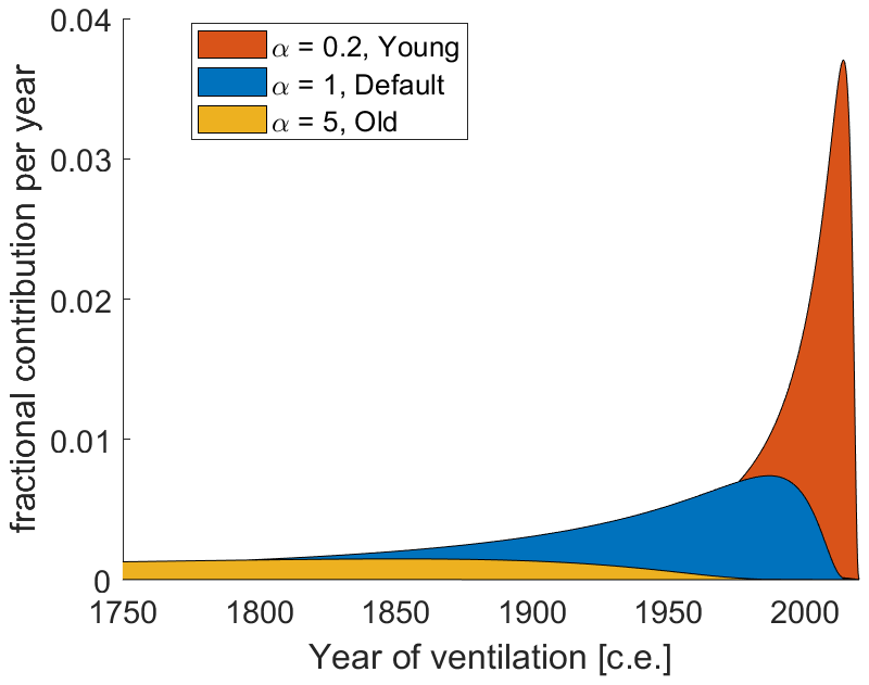
Figure 2 Three example ventilation-year distributions for a parcel of water observed in the year 2020. The “young,” “default,” and “old” mixtures in orange, blue, and yellow have mean ages of ∼17, 91, and 460 years, respectively. Fractions of a given color add up to 1 when summed across all years.

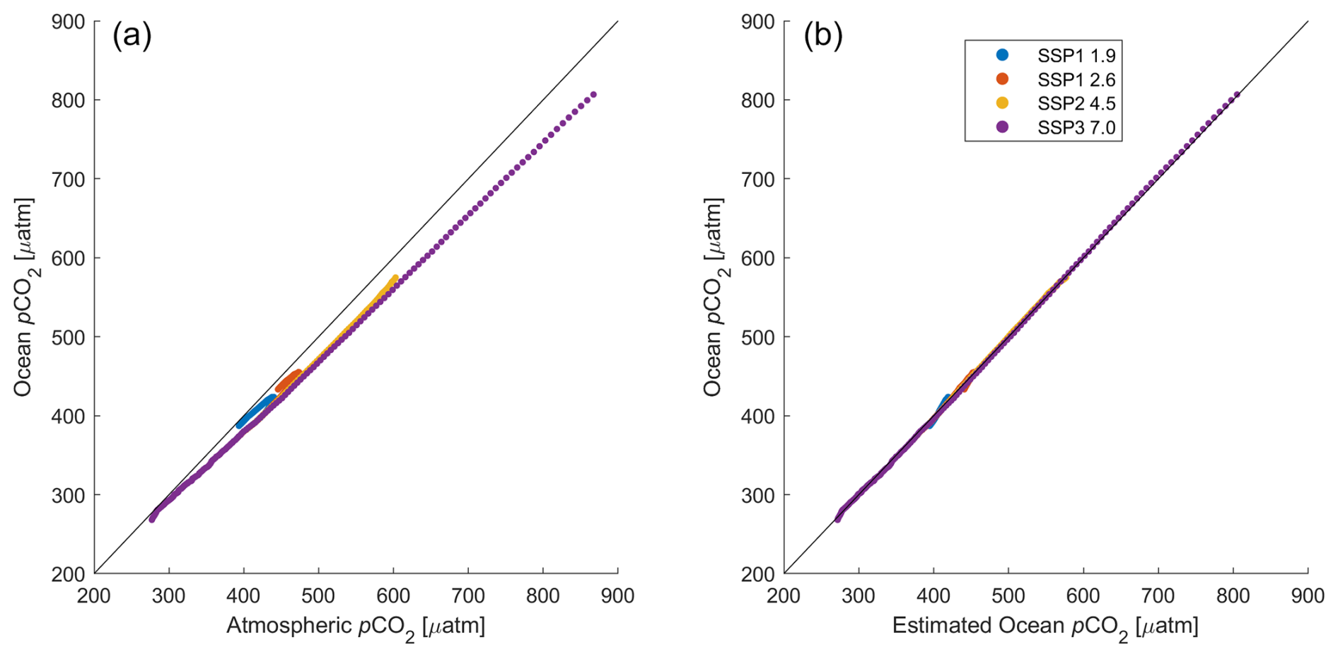
Figure 3 A comparison between surface ocean pCO₂ values in the model-based data product of Jiang et al. (2023) and (a) the modeled atmospheric XCO₂ value and (b) the value obtained from Eq. (5). Black 1:1 lines are provided for reference, and the colored dots indicate projected and historical values from four different SSPs.

Once the age distribution is known, the atmospheric CO₂ record is convoluted into the age distribution as outlined as follows (Hall et al., 2002): first, the atmospheric record or projection is interpolated to obtain values for the year of the desired estimate minus the ages in the distribution. Then, for each of the (up to) 1000 fractions of the water mass, the fraction-weighted mean ages ($\stackrel{\mathrm{‾}}{A}$) and concentrations ($\stackrel{\mathrm{‾}}{\left[X\right]}$) can be computed as fraction-weighted sums. For example, for gas X with atmospheric concentration [X] summed over the $i=\mathrm{1}:\mathrm{1000}$ years prior to the estimate of interest, this would be computed as follows:

$$\begin{array}{}\text{(4)}& \stackrel{\mathrm{‾}}{\left[X\right]}=\sum _{i=\mathrm{1}}^{\mathrm{1000}}{f}_i[X{]}_i.\end{array}$$

For the $\stackrel{\mathrm{‾}}{A}$ calculation, [X_i] is replaced in this equation with i years. The concentration values reflect complete air–sea equilibration, which is inconsistent with net ocean uptake of CO₂ from air–sea gas exchange. For example, in the RECCAP2 model simulations, there is a 108±4 µatm increase in the surface ocean pCO₂ in 2018 relative to the preindustrial value compared to a 128.72 mol mol⁻¹ change in the atmospheric XCO₂ (DeVries et al., 2023; Müller, 2023). Also, the air–sea CO₂ disequilibrium is thought to vary temporally (He et al., 2018) and be sensitive to the rate of atmospheric XCO₂ change. Therefore, we derive an empirical relationship between atmospheric XCO₂ and the median model–observation hybrid apparent surface ocean pCO₂ record given by Jiang et al. (2023). A variety of predictive relationships were tested, and the strongest predictive relationship (lowest root-mean-square error, RMSE) was obtained for the following:

$$\begin{array}{}\text{(5)}& \begin{array}{rl}p{\mathrm{CO}}_{\mathrm{2},\mathrm{oce}.\mathrm{year}}& =X{\mathrm{CO}}_{\mathrm{2},\mathrm{atm}.\mathrm{year}}-\mathrm{0.144}\\ & \cdot \left(X{\mathrm{CO}}_{\mathrm{2},\mathrm{atm}.\mathrm{year}}-X{\mathrm{CO}}_{\mathrm{2},\mathrm{atm}.\mathrm{year}\mathrm{\_}\mathrm{minus}\mathrm{\_}\mathrm{65}}\right).\end{array}\end{array}$$

Equation (5) suggests that the expected surface ocean pCO₂ value in an arbitrary year pCO${}_{\mathrm{2},\mathrm{oce}.\mathrm{year}}$ can be estimated as a function of the atmospheric XCO₂ in that year (XCO${}_{\mathrm{2},\mathrm{atm}.\mathrm{year}\mathrm{\_}\mathrm{minus}\mathrm{\_}\mathrm{65}}$) and the difference between that atmospheric value and the value in the atmosphere 65 years prior (XCO${}_{\mathrm{2},\mathrm{atm}.\mathrm{year}}$). Applying Eq. (5) to the XCO₂ record before use in TRACEv1 meaningfully reduces the mismatch between the simulated surface ocean pCO₂ and the atmospheric XCO₂ (Fig. 3). An additional constant offset of −5.37 µatm was found in the best-fit relationship (not shown on the right-hand side of Eq. 5), but this term likely reflects the water vapor correction between XCO₂ and pCO₂ and, potentially, parameterized net model degassing of riverine carbon. TRACEv1 neglects this constant offset because the code separately applies the water vapor correction for each parcel of seawater (Dickson et al., 2007) when converting between XCO₂ and pCO₂ and because including this term would have a nearly identical impact on preindustrial pCO₂.

Once water-fraction-weighted mean pCO₂ values $\stackrel{\mathrm{‾}}{p{{\mathrm{CO}}_{\mathrm{2}}}_{\mathrm{oce}.}}$ are estimated for a parcel of seawater, the expected equilibrium DIC value for the water parcel when last at the ocean surface is calculated using estimated TA⁰, Si⁰, and P⁰. These calculations are repeated with both the $\stackrel{\mathrm{‾}}{p{{\mathrm{CO}}_{\mathrm{2}}}_{\mathrm{oce}.}}$ and a user-provided preindustrial XCO₂ value (default is 280 ppm, adjusted for water vapor), and their difference is attributed to C_anth. During fitting of the α values (described later), a similar procedure is followed for transient tracer observations with CFC and SF₆ equilibrium constants (see Warner and Weiss, 1985, and Bullister et al., 2002, respectively), although without adjustments for incomplete equilibration because the equilibrium timescales for these tracers are shorter than for CO₂.

Carbonate chemistry calculations are computed with the CO2SYS code written for MATLAB (Van Heuven et al., 2011) and modified herein to increase the tolerance for pH changes during iteration from 0.0001 to 0.001 when converging on a pH value (to speed up the calculation). Carbonate dissociation constants from Lueker et al. (2000) are used with the total boron calculation from Uppström (1974) and the K_F calculation from Perez and Fraga (1987). S and T values that are outside the viable range for these carbonate chemistry constants (S=19–48 and T=2–35 °C) are overridden with the nearest viable S and T values. This override has a minimal impact on most C_anth calculations for common seawater types, but we caution here that TRACEv1 is not intended for use in freshwater or brackish environments. Information on computing optimization is provided in Sect. S4.

2.3 Data and model output used to train and run TRACEv1

The α parameter is fit to the CFC-11, CFC-12, and SF₆ partial pressures that would be found in a gas phase in complete air–sea equilibrium with seawater with the measured composition, as well as to A from the Ocean Circulation Inverse Model (OCIM) transport matrix (John et al., 2020) when the zero-age boundary layer is set equal to the shallowest layer in the OCIM model. For the real ocean, the transient tracer partial pressure values are taken as calculated from discrete seawater measurements in the GLODAPv2.2023 data product (Lauvset et al., 2024). Co-located measurements of salinity and temperature are also extracted from this data product. For the model reconstruction test, C_anth, S, and T are taken from or computed from the NorESM RECCAP2 simulations (Müller, 2023). In addition to the standard RECCAP2 outputs, this model was also used to simulate CFC-11, CFC-12, and SF₆ through the start of 2015 (Schwinger, 2024). The approaches used to obtain scattered values from gridded model output and to obtain scattered ages from the OCIM transport matrix are given in Sect. S5.

TRACEv1 allows more than nine options for atmospheric CO₂ projections/histories and relies on a single reconstruction of transient tracers taken from a data product compiled by the United States Geological Survey (USGS) Reston Groundwater Dating Laboratory (see the “Data availability” section). The atmospheric XCO₂ reconstruction starting in the year 1 and continuing through the year 1000 is taken from the synthesis by Frank et al. (2010) for all CO₂ options. Before the year 1, all reconstructions are set to a constant value of xCO₂=277.14 ppmv, equaling the atmospheric concentration in the year 1. From 1001 and through 1959, all reconstructions follow the historical concentrations of the SSPs as defined by Meinshausen et al. (2020), which are identical over this time range. From 1959 through 2022, the first option, which is called “historical/linear” and is the default option if no alternative is specified, uses the Mauna Loa measurements by Keeling et al. (1976) and Thoning et al. (1989), and if TRACEv1 is instructed to use this record to generate an estimate for a year that is after 2022, the slope from a linear trend fit to the last 10 years of the historical record is used to project to the year of the desired estimate. The remaining eight options are SSP1-1.9, SSP1-2.6, SSP2-4.5, SSP3-7.0, SSP3-7.0-lowNTCF, SSP4-3.4, SSP4-6.0, and SSP5-3.4-over, all as defined by Meinshausen et al. (2020). The SSPs diverge from each other starting in 2017. Between the years 1959 and 2017, the SSP values have a small average bias of +0.6 ppmv compared to the historical Mauna Loa measurements with a root-mean-square disagreement of 0.8 ppmv. Additional custom concentration pathway options can be added by appending a new column of atmospheric CO₂ concentrations to a plain text file (CO2TrajectoriesAdjusted.txt) that is read by TRACEv1 and by entering the number of the new option in the TRACEv1 code (i.e., if a 10th option is added, the CO₂ pathway option for the “AtmCO2Trajectory” input would be 10). However, any user-provided concentration pathways should be adjusted by Eq. (5) before appending them to this file.

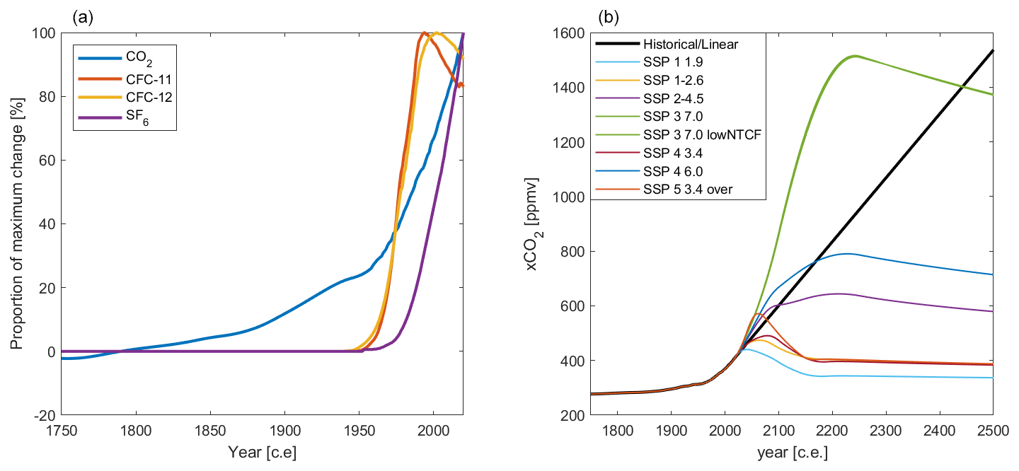
Figure 4 (a) The time history of atmospheric transient tracer and CO₂ concentrations expressed as a percentage of their maximum deviation through 2020 from their assigned preindustrial values of 0 ppmv for CFC-11, CFC-12, and SF₆ and 280 ppmv for CO₂.(b) The nine atmospheric CO₂ concentration pathway options used by TRACEv1, with all but “historical/linear” being SSPs as given by Meinshausen et al. (2020). Both versions of SSP3-7.0 fall nearly on top of each other on this plot and are assigned the same colors.

2.4 Fitting TRACEv1 parameters

The parameters are optimized using a bounded minimum “search” function (“fminsearchbnd” in MATLAB) with an initial value of α=1, an upper bound of α=1000, and a lower bound of α=0.001. This function uses a Nelder–Mead simplex algorithm (Lagarias et al., 2006) with iterative variations in the α term by 5 % to minimize a cost function. For each iteration of this solver, the j=3 (i.e., CFC-11, CFC-12, and SF₆) transient tracer constraints and the A are first calculated as described in Eq. (4). The cost function that is minimized for this solver (ε²) is the sum of the squared normalized errors of the three partial pressures and A, or

$$\begin{array}{}\text{(6)}& {\mathit{\epsilon }}^{\mathrm{2}}=\sum _{j=\mathrm{1}}^{\mathrm{3}}{\left({\displaystyle \frac{p{X}_{\mathrm{meas}}^j-p{X}_{\mathrm{calc}}^j}{p{X}_{\mathrm{ATM}}^j}}\right)}^{\mathrm{2}}+{\left({\displaystyle \frac{A_{\mathrm{OCIM}}-A_{\mathrm{calc}}}{A_{\mathrm{Max}}}}\right)}^{\mathrm{2}}.\end{array}$$

Here, $p{X}_{\mathrm{meas}}^j$ is the measured partial pressure of transient tracer j extracted from discrete GLODAPv2.2023 product or (for the model validation experiments) from GOBM output, $p{X}_{\mathrm{calc}}^j$ is the value calculated from α and the record of atmospheric trace gas concentrations as described above, and $p{X}_{\mathrm{ATM}\mathrm{\_}\mathrm{2020}}^j$ is the atmospheric partial pressure of tracer j in the year 2020. This third term is included to normalize the errors to a more comparable scale. Without this term, the pCFC-12 (SF₆) errors would be assigned higher (lower) weight than the errors in the other two transient tracers due to their greater (smaller) atmospheric partial pressures. Similarly, A_OCIM is the interpolated OCIM age, A_calc is the calculated A, and A_max is the ideal age of the oldest grid cell found in the OCIM age calculations (1354 years).

This process is repeated for the observational record and for the model output. The version of TRACEv1 that is trained on model output is referred to as TRACEv1_validation_NorESM, and details of this comparison are provided in Sect. S6. The version trained on real-world observations is referred to as TRACEv1. We generate 10 versions of TRACEv1 in which we retrain TRACEv1 after perturbing the transient tracer measurements from each cruise in GLODAPv2.2023 by a cruise-wide relative offset and each measurement by measurement-specific random perturbations. In Sect. S7, we quantify the likely impact of measurement uncertainties in the transient tracer measurements on the final C_anth estimates via Monte Carlo analysis.

2.5 C_anth data product creation

We use the gridded, temporally averaged GLODAPv2 data product (Lauvset et al., 2016) for S, T, latitude, longitude, and depth and vary only the year of the estimate to equal {1750, 1800, 1850, 1900, 1950, 1980, 1994.5, 2000, 2002, 2007.5, 2010, 2014.5, 2020, 2030, 2050, and 2100}. Estimates are only made using the historical/linear and SSP1-1.9 reconstructions prior to 2010 (and we note that the SSPs are identical over this period). In 2020 and thereafter, estimates are provided for each of the nine CO₂ concentration pathway options separately. The estimates in 1994.5, 2002, 2007, and 2014 are provided for comparison and interoperability with published literature distributions (Gruber et al., 2019a; Lauvset et al., 2016; Müller et al., 2023; Sabine et al., 2004).

We anticipate that the small differences between the 1750 and 1850 CO₂ concentration estimates could prove useful for reconciling literature estimates of C_anth that have been made to be specific to these two common choices of reference year. Our C_anth definition is specific to the 280 ppmv atmospheric concentration rather than to a specific year. It is therefore possible for TRACEv1 to return very small negative C_anth values, particularly for estimates following periods in which CO₂ reached minima of $\sim \mathrm{277}\pm \mathrm{1}$ ppmv in the 1st, 6th, and 18th centuries CE. The last time the atmospheric CO₂ concentration was believed to equal 280 ppmv was 1790 (Frank et al., 2010), and TRACEv1 allows users to specify an alternative reference concentration.

3 Results and discussion

We discuss the uncertainty assessment and compare TRACEv1 reconstructions to alternatives, discuss the TRACEv1 projections through 2500, and highlight some areas where TRACEv1 is limited and might be improved. We compare TRACEv1 A estimates to alternatives in Sect. S8.

3.1 Uncertainty estimation

In Sect. S5, we describe the results of our uncertainty assessments from model reconstruction (subscript MR) C_anth distributions. In Sect. S6, we present the results of the Monte Carlo (subscript MC) analysis. Here, we combine the results of these analyses to estimate the uncertainty of TRACEv1 (U_TRACEv1) estimates that results from several sources. The model C_anth reconstruction estimates reveal methodological uncertainties, including the limitations of an IG TTD and the inaccuracies associated with using a neural network across a large geographical area, and the uncertainties that result from potential OCIM A distribution and preformed property distribution errors. The Monte Carlo analysis reveals uncertainties that result from random uncertainties and cruise-wide offsets in transient tracer concentration measurements. We add these uncertainties in quadrature to obtain the overall uncertainty estimate (±1σ) for TRACEv1 (U_TRACEv1):

$$\begin{array}{}\text{(7)}& U_{\mathrm{TRACEv}\mathrm{1}}=\sqrt{u_{\mathrm{MC}}^{\mathrm{2}}+u_{\mathrm{MR}}^{\mathrm{2}}}.\end{array}$$

Here, u_MC is the Monte Carlo RMSE estimate of 1 µmol kg⁻¹ for C_anth and ±0.3 % for inventories, and u_MR is the uncertainty estimate from the model reconstruction of 4.4 µmol kg⁻¹ for C_anth and 15 % for inventories, conservatively chosen because the model reconstruction reproduces inventories to within 10 % in 1980 and 2014. The uncertainty appears to grow with the estimate and over time, so 15 % of the estimated C_anth is used when this value exceeds 4.4 µmol kg⁻¹. These uncertainty estimates neglect the contribution of uncertainty in the S and T values used in the neural network to the overall C_anth estimate uncertainty, which we believe to be small relative to U_TRACEv1, but we note that users can conduct perturbation tests if they are supplying particularly uncertain S and T information. U_TRACEv1 is an optional output from TRACEv1. In Sect. S6, we show that reconstruction errors are significantly larger in marginal seas with few or no transient tracer measurements and are also elevated near coasts and in areas of strong upwelling. U_TRACEv1 should be considered an underestimate in these regions. We do not attempt to estimate uncertainty in the optional A TRACEv1 output.

3.2 C_anth reconstructions and data product comparisons

The reconstructions and projections from TRACEv1 (Table 1) match past anthropogenic inventory estimates obtained from analyses based on measurements of DIC changes and distributions (Fig. 5) in 1994 (118(±26) PgC from Sabine et al., 2004, vs. 127(±19) for TRACEv1), 2007 ($\mathrm{118}(\pm \mathrm{26})+\mathrm{29}(\pm \mathrm{2.5})=\mathrm{147}(\pm \mathrm{26})$ PgC from Müller et al., 2023, updating Gruber et al., 2019a, vs. 161(±24) for TRACEv1), and 2014 ($\mathrm{118}(\pm \mathrm{26})+\mathrm{29}(\pm \mathrm{2.5})+\mathrm{27}(\pm \mathrm{2.5})=\mathrm{174}(\pm \mathrm{26})$ PgC from Müller et al., 2023, vs. 182(±27) for TRACEv1). The agreement with the DIC-based approaches is reassuring, as there is little overlap in the data or methodologies used to generate the DIC-based estimates compared to the data and methods used to obtain the TRACEv1 routines: Müller et al. (2023) did not rely on transient tracer information, and the data used in this study are, on average, more recent than the CFC-11 and CFC-12 information used by Sabine et al. (2004) (Fig. 1).

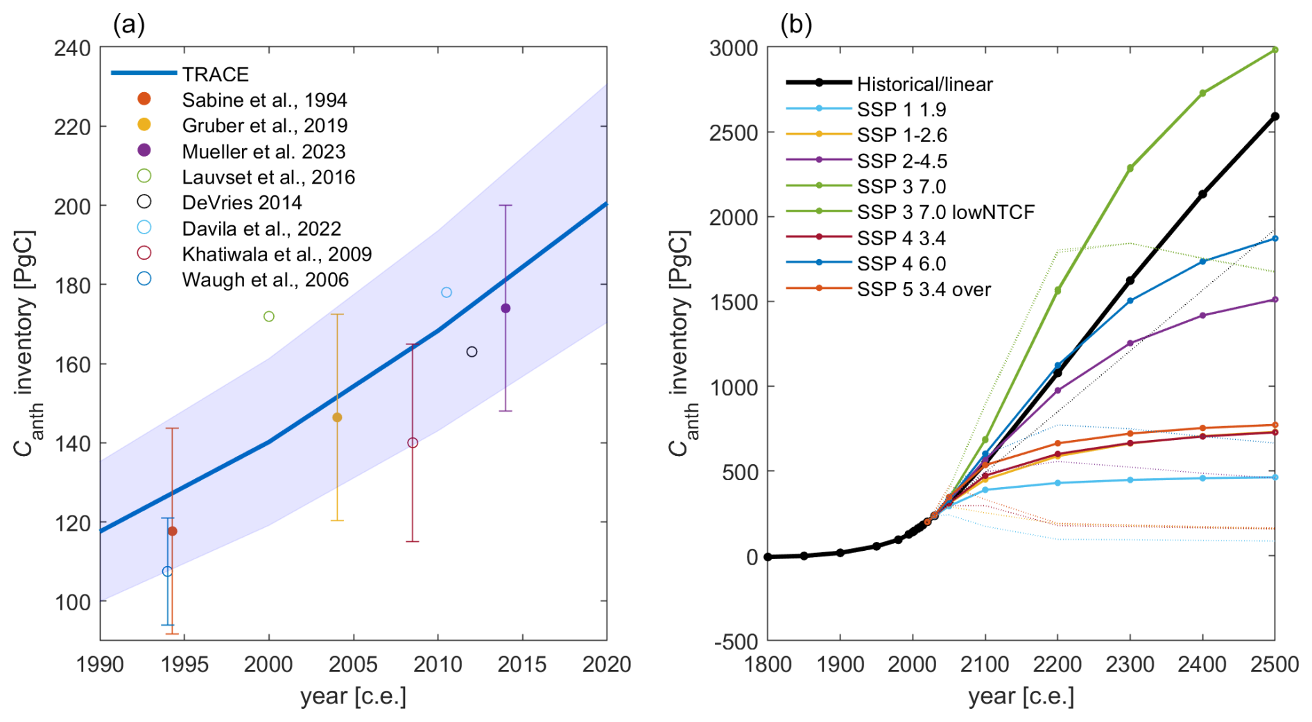
Figure 5 Panel (a) shows the global C_anth inventory projected by TRACEv1, with blue shading indicating the uncertainty estimate. Circles show estimates from literature-data-based C_anth distribution estimates, with filled circles indicating estimates rooted primarily in DIC measurements and open circles indicating estimates rooted primarily in fitting transient tracer distributions. Panel (b) shows projected values through 2500, using solid lines for various SSPs (as labeled). Thin dotted lines indicate the inventories that would be obtained by projecting the 2020 estimate using transient steady-state assumptions (Gammon et al., 1982) with the atmospheric CO₂ concentrations from the SSPs with the same line color. Both versions of SSP3-7.0 fall nearly on top of each other on this plot and are assigned the same colors.

Table 1 TRACEv1 estimates of C_anth inventories (in PgC ± 1σ uncertainties) calculated by ocean basin for the specified points in time. The Atlantic becomes the Arctic at 40° N, whereas the Pacific transitions at 67° N. The Southern Ocean is defined as the area in all basins south of 40° S. Anthropogenic inventories are small and negative in 1750 because of the ∼200-year-long period with a <280 ppmv CO₂ atmosphere prior to the industrial era.

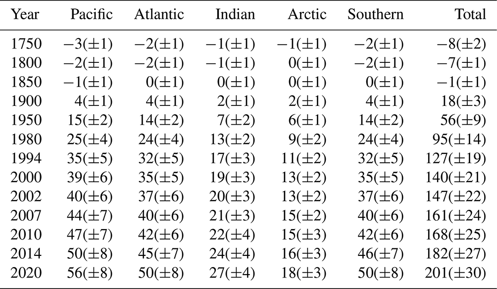
The regional distribution of the C_anth inventory qualitatively matches prior estimates as well, with significantly higher column inventory estimates in the North Atlantic (Fig. 6, Table 1). Similarly, there are areas of higher column inventories generally in the Southern Hemisphere portions of the other ocean basins, as mode and intermediate waters are exported northward from the Southern Ocean. Within Fig. 6, bathymetric features such as the Kerguelen Plateau and the Mid-Atlantic Ridge are visible when they displace waters that would otherwise contain meaningful quantities of C_anth, and a band of low column inventories can be seen within the Antarctic Circumpolar Current where old deep waters upwell to near the ocean surface.

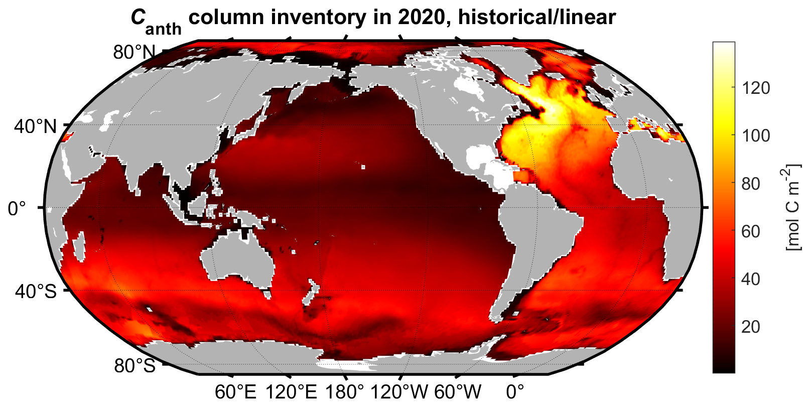
Figure 6 Column inventory of C_anth mapped for 2020 using TRACEv1 with the historical/linear atmospheric CO₂ pathway.

TRACEv1 has a more variable agreement with estimates based on transient tracer information. The estimates are higher than – but within uncertainties of – the Green function fits of Khatiwala et al. (2009) and a TTD-based inventory estimate (Waugh et al., 2006). TRACEv1 estimates of 168(±25) PgC are within uncertainties of the 178 PgC inventory of Davila et al. (2022) calculated in 2010 using the total matrix intercomparison approach. At 172(±26) PgC, TRACEv1 estimates are near the OCIM estimates of Devries (2014) of 160–166 PgC in 2012, although this not surprising because the A estimates implied by an OCIM solution were used as a fitting parameter for TRACEv1. The TTD-based C_anth inventory for 2002 in the gridded GLODAPv2 data product of Lauvset et al. (2016) is 179 PgC compared to a TRACEv1 estimate of 147(±22) PgC in the same year. In Sect. S9, we show that the main disagreement between the TRACE estimates and the GLODAPv2 gridded product (Lauvset et al., 2016) is found in the deep ocean, where GLODAPv2 inventories consistently exceed TRACE inventories below ∼500 m. There are several possible reasons for this disagreement, but the true cause is unclear.

3.3 C_anth inventory projections

The C_anth inventory projections (Table 2, Fig. 5b) indicate that, even if humanity acts to rapidly reduce C_anth in the atmosphere and manages to bring atmospheric XCO₂ down to 337 µatm by the middle of the millennium in line with the ambitious SSP1-1.9 scenario, the ocean will never – on this time horizon – cease to take up additional C_anth, picking up an additional 5.4 PgC between 2400 and 2500. This builds on the findings of Koven et al. (2022) and Jones et al. (2016) using full model simulations through 2300 and suggests that the impacts of ocean acidification are likely to continue to spread throughout the ocean depths, even with a highly successful carbon management policy. Nevertheless, such action remains important for preventing ocean acidification, as the degree of surface and interior ocean acidification depends strongly on which SSP we follow. This is particularly true for the well-lit surface euphotic zone that is the base of most marine food webs: the relative proportion of marine C_anth shifts increasingly from the surface ocean to the ocean depths over time (Fig. 7a), and this tendency becomes more pronounced the more rapidly and completely that atmospheric CO₂ emissions are curtailed and reversed (Fig. 7b). Indeed, several SSPs show reduced surface C_anth relative to modern values despite the continued ocean C_anth accumulation. An important caveat is that these findings do not consider the impacts of changes in heat and freshwater content, circulation, or changes in the ocean's biological pump; rather, they only reflect the impact expected from changing atmospheric XCO₂ and the oceanic buffering capacity.

Table 2 TRACEv1 projections of global ocean C_anth inventories (in PgC) until the middle of the millennium if the indicated atmospheric CO₂ concentration pathway is followed.

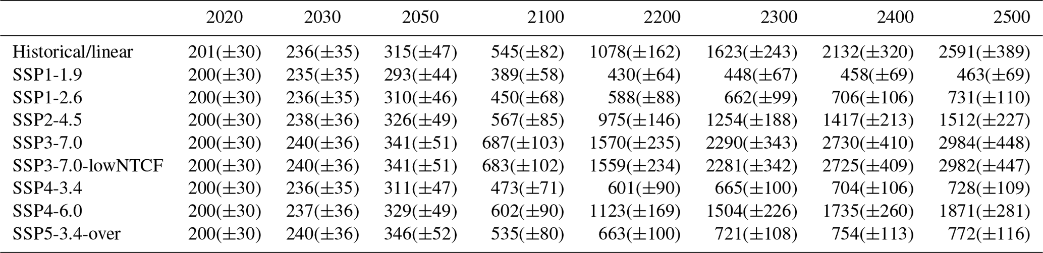
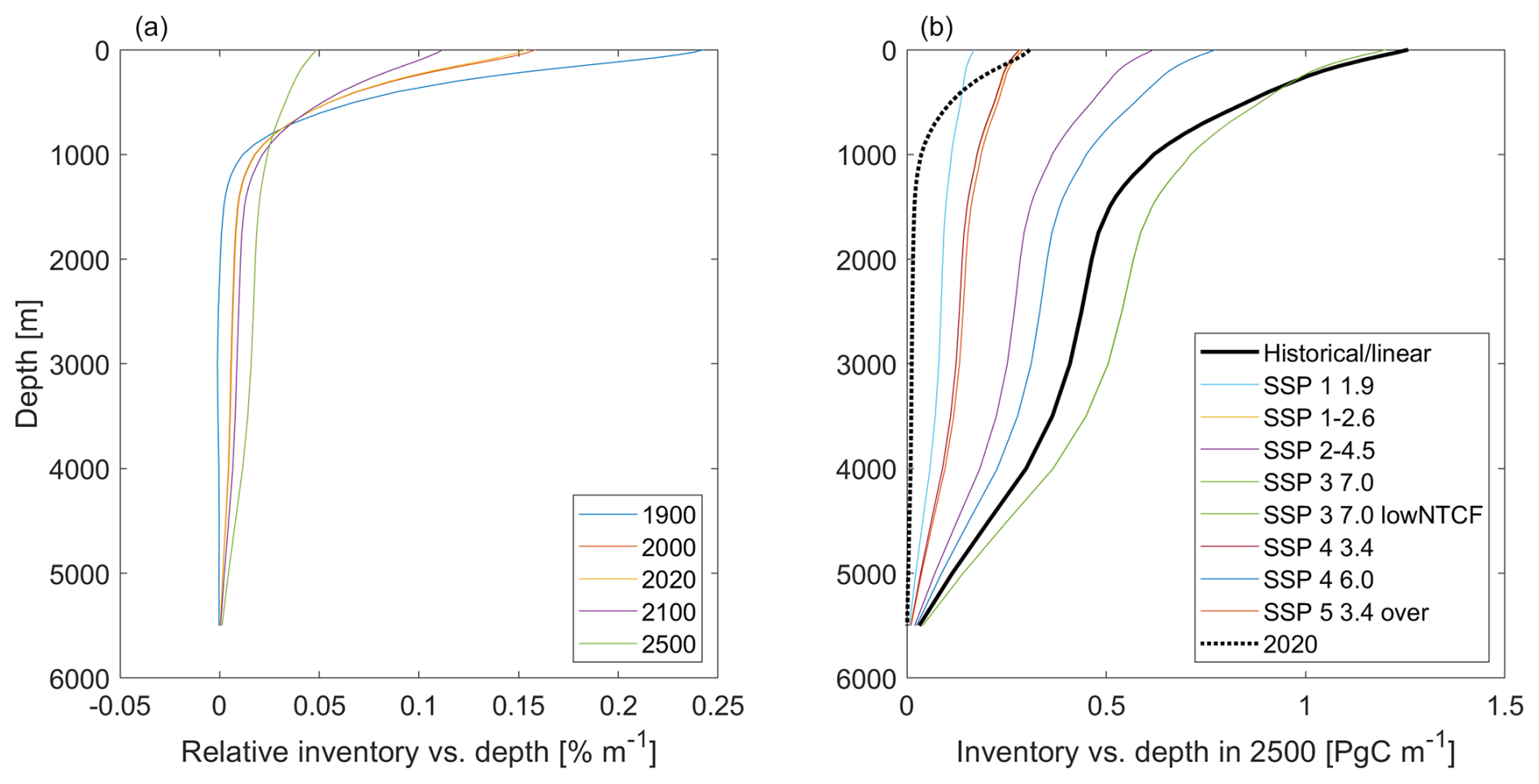
Figure 7 (a) The relative inventory of C_anth vs. depth in various years of the historical/linear projection, expressed as the percentage of the total DIC inventory that is found within each 1 m interval. Here, a shrinking surface value indicates that a greater proportion of the signal is found at depth, but it does not necessarily imply a lower surface C_anth. Panel (b) shows the total inventory in 2500 vs. depth using solid lines for each of the CO₂ concentration pathways employed by TRACEv1, with the 2020 historical/linear inventory plotted as a dashed line for comparison. Both versions of SSP3-7.0 fall nearly on top of each other on this plot and are assigned the same colors.

One intended use for TRACEv1 is adjusting the DIC measurement to a reference year. The simple approximation of a transient steady state (Gammon et al., 1982) has been used in several recent studies (e.g., Lauvset et al., 2016; Clement and Gruber 2018; Carter et al., 2021a; Müller et al., 2023), and our projections show that this assumption performs plausibly for projections over short timescales. However, we contend that TRACEv1 provides a superior means of adjusting DIC measurements to be appropriate for a reference year. For example, the differences between modeled C_anth between 1980 and 2014 in NorESM disagree with the differences between TRACEv1 estimates for those same years by an average of $-\mathrm{0.1}(\pm \mathrm{3.0})$ µmol kg⁻¹. The statistics are worse at $-\mathrm{1.2}(\pm \mathrm{3.6})$ µmol kg⁻¹ when modeled differences are compared instead to the differences between the 1980 C_anth values and the 1980 values scaled to 2014 using transient steady-state assumptions. Thus, both adjustments are reasonable from 1980 to 2014, but the transient steady-state adjustment tends to overpredict the change. Also, unlike TRACEv1, transient steady-state adjustments require an independent estimate of C_anth. (For the comparison above, they were provided the exactly correct model C_anth distribution in the earlier year, although this is never known in the real ocean.) Finally, the transient steady-state assumption is also known to break down if the atmosphere ceases to increase in its tracer concentration exponentially; this occurs by 2500 for CO₂ in all SSPs, although most SSPs reach this point much sooner (Meinshausen et al., 2020). It can be seen in these cases that a transient steady state results in large errors in the projected C_anth inventories by mid-millennium and even projects spurious decreases (Fig. 5b).

3.4 Limitations and future directions

There are several notable limitations of the TRACEv1 method:

1. It presumes fixed circulation and is unable to resolve most timescales and modes of C_anth variability.

2. It shows larger reconstruction errors in regions that lack training data, which is a common problem for neural networks and other regression strategies (e.g., Carter et al., 2021a). As transient tracer measurements with the strong SF₆ constraint are still relatively rare (approximately 5 % of the GLODAPv2.2023 data product contains all three transient tracer measurements), it is likely that TRACE will improve as more such measurements become incorporated. However, version 1 of TRACE should be used with caution in regions without training data, and this caution applies to many marginal seas (Fig. 1 and Fig. S1 in the Supplement).

3. TRACEv1 appears to overestimate C_anth in surface waters where there is meaningful upwelling, although perhaps not by a larger extent than alternative C_anth estimation strategies. This is unfortunate because such surface waters are frequently found in areas of naturally low pH that are of interest for ocean acidification research.

4. The method has not yet been well validated in a high-resolution model representation of a coastal environment, so its uncertainties are not well estimated outside of the open ocean. While the circulation information encoded in TRACEv1 has been optimized within a limited parameter space, it is likely – based on past literature exploring many options for simplifying the complex distributions of myriad water types that mix in the ocean interior – that the comparatively simple single term that we employ herein to constrain interior ocean age distributions could be meaningfully improved. We leave this to future work.

5. Furthermore, the TTD approach is limited by the need for an assumed air–sea disequilibrium and the possibility that the degree of disequilibrium for transient tracers varies meaningfully over time and space and between CFCs and SF₆ (Shao et al., 2013; Sonnerup et al., 2015) and differs from the related term for air–sea CO₂ disequilibria, which seems likely due to the slow relaxation of CO₂ disequilibria (Jones et al., 2014) and the faster rate of transient tracer equilibration (Wanninkhof, 2014). A common assumption of 100 % equilibration tends to result in TTD approaches overestimating C_anth (Waugh et al., 2006). We include an empirical relationship intended to deal with this issue but note that its formulation remains somewhat ad hoc and based on model simulations of surface ocean conditions.

6. TRACEv1 is aimed at resolving the accumulation of C_anth under steady-state circulation. However, it is possible that it is able to resolve some non-steady-state components of C_anth accumulation when it is called with time-varying temperature and salinity records as predictors. It is yet untested to what degree this is an effective strategy for capturing such variability.

We include the version number in TRACEv1 both to signal that future improvements are likely and to disambiguate the function from other software routines that might have similar names. There are several ways that TRACEv1 might be improved:

1. Some fitting strategies have shown improvements when the signal of interest is fit to the disagreement between observations and a model prior, instead of being fit directly to the signal. This approach could improve estimates if a model prior age distribution can be obtained and be regridded to global locations of interest in a computationally efficient manner.

2. Further optimization of the shape of the TTD could result in improved C_anth reconstructions.

3. MATLAB is an open-source language, but it is not freely available. It would therefore further improve the accessibility of C_anth estimates if TRACEv1 were released in a freely available computing package. Prior experience suggests that a modest amount of script is required to convert neural networks from MATLAB to Python, whereas somewhat less script is required to transition the code to Julia. This is left to future work.

4 Data availability

The gridded GLODAP product is available at https://glodap.info/ (GEOMAR and the ICOS Ocean Thematic Center, 2024). The CFC and SF₆ atmospheric record data product was obtained from the USGS Reston Groundwater Dating Laboratory website: https://water.usgs.gov/lab/software/air_curve/index.html (U.S. Department of the Interior and U.S. Geological Survey, 2025). The TRACEv1_GGC_anth product is available from Zenodo: https://doi.org/10.5281/zenodo.15003059 (Carter, 2025). The NorESM modeled distributions of transient tracers are also available from Zenodo: https://doi.org/10.5281/zenodo.14536027 (Schwinger, 2024). TRACEv1 data can be found and freely obtained at https://doi.org/10.5281/zenodo.15692788 (BRCScienceProducts, 2025).

5 Code availability

TRACEv1 code can be found and freely obtained at https://doi.org/10.5281/zenodo.15692788 (BRCScienceProducts, 2025).

6 Conclusions

We present a new method called TRACEv1 for rapidly estimating the time-varying C_anth distribution throughout the open ocean, including detailed error estimates. TRACEv1 is available as a function in the MATLAB programming language. We further provide a data product with C_anth distributions for a range of years (TRACEv1_GGC_anth; Carter, 2025) on the GLODAPv2 gridded product grid used by Lauvset et al. (2016). We use this data product to examine how the C_anth distribution varies with depth and time, and we show that the ocean can be expected to continue to increase its C_anth inventory through 2500 for all SSPs. We find that SSP3-7.0 results in the largest projected 2500 ocean C_anth inventory of 2984(±448) PgC, and this represents a ∼15-fold increase over the 2020 C_anth inventory.

There are several strengths of the TRACEv1 method, which relies on TTDs to estimate C_anth distributions from a time-evolving atmospheric CO₂ trajectory. The method is easy and quick to implement, shows fidelity to model reconstructions and agreement with recently published data-based estimates, and only requires S and T measurements and spatiotemporal coordinate information to produce an estimate. It also provides means to plausibly adjust collections of DIC measurements collected over time to a common time by removing the influences of C_anth changes. While the reconstruction fidelity of TRACEv1 estimates were quite high in a test using model output with exactly known C_anth distributions, we nevertheless believe the primary advantage of TRACEv1 and the new data product is their accessibility.