A global daily seamless 9 km vegetation optical depth (VOD) product from 2010 to 2021

Vegetation optical depth (VOD) products provide information on vegetation water content and correlate with vegetation growth status; these are closely related to the global water and carbon cycles. The L-band signal penetrates deeper into the vegetation canopy than the higher-frequency bands used for many previous VOD retrievals. Currently, there are only two operational L-band sensors aboard satellites, i.e., the Soil Moisture and Ocean Salinity (SMOS) satellite launched in 2010 and the Soil Moisture Active Passive (SMAP) satellite launched in 2015. The former has the limitation of a low spatial resolution of only 25 km, while the latter has improved this resolution to 9 km but has a shorter usable time range. Due to the influence of sensor and atmospheric conditions as well as the observation methods of polar-orbiting satellites (such as scan gaps and observation revisit times), the daily data provided by both satellites suffer from varying degrees of missing data. In summary, the existing L-band VOD (L-VOD) products suffer from the defects of missing data and coarse resolution of historical data. There is little research on filling gaps and reconstructing 9 km long-term data for L-VOD products. To solve this problem, our study depends on a penalized least-square regression based on a three-dimensional discrete cosine transform to firstly generate the seamless global daily L-VOD products. Subsequently, the nonlocal filtering idea is applied to spatiotemporal fusion between high-resolution and low-resolution data, resulting in a global daily seamless 9 km L-VOD product from 1 January 2010 to 31 July 2021. In order to validate the quality of the products, time series validation and simulated missing-region validation are used for the reconstructed data. The fusion products are validated both temporally and spatially and are also compared numerically with the original 9 km data during the overlapping period. Results show that the seamless SMOS (SMAP) dataset is evaluated with a coefficient of determination (R²) of 0.855 (0.947) and a root mean squared error (RMSE) of 0.094 (0.073) for the simulated real missing masks. The temporal consistency of the reconstructed daily L-VOD products is ensured with the original time series distribution of valid values. The spatial information of the fusion product and the original 9 km data in the overlapping period is basically consistent (R²: 0.926–0.958, RMSE: 0.072–0.093, and mean absolute error MAE: 0.047–0.064). The temporal variations between the fusion product and the original product are largely synchronized. Our dataset can provide timely vegetation information during natural disasters (e.g., floods, droughts, and forest fires), supporting early disaster warning and real-time responses. This dataset can be downloaded at https://doi.org/10.5281/zenodo.13334757 (Hu et al., 2024).

1 Introduction

Vegetation is a key factor in the energy, water, and carbon balance of the terrestrial surface, and it is significantly affected by climate change and human activities (Frappart et al., 2020). Remote sensing observations are commonly used to monitor vegetation dynamics and their temporal changes from regional to global scales. Unlike traditional optically based technologies, microwave-frequency sensors are almost unaffected by cloud cover (Moesinger et al., 2020). Microwave radiation passing through the vegetation canopy undergoes an extinction effect, and the extent of this attenuation can be observed by passive or active microwave satellites and is commonly referred to as vegetation optical depth (VOD) (Wigneron et al., 2017). It is increasingly used to monitor various ecological vegetation variables, which can provide frequent observations that are independent of atmospheric conditions and cloud pollution. Soil moisture contribution is coupled to the effects of vegetation in terms of absorption and scattering (Zhao et al., 2021; Liu et al., 2012), and water within the vegetation attenuates the microwave signal (Yao et al., 2024). Thus, VOD is directly related to the vegetation water content (VWC) (Fan et al., 2019; Konings et al., 2016; Dou et al., 2023; Holtzman et al., 2021). VOD has been widely used in biomass monitoring, drought early warning, phenology analysis, and other fields (Wigneron et al., 2020; Vreugdenhil et al., 2022; Moesinger et al., 2022; Kumar et al., 2021; Van Dijk et al., 2013; Ferrazzoli et al., 2002; Vaglio Laurin et al., 2020; Mialon et al., 2020; Fan et al., 2023). VOD is affected by a number of factors, including density, type of vegetation, and microwave frequency. Many microwave remote sensing satellites provide VOD products in different microwave bands (X, Ku, and C). However, as the frequency of the microwave signal decreases, resulting in longer wavelengths, its ability to penetrate vegetation canopies increases (Frappart et al., 2020; Zhang et al., 2021a). Compared to VOD products in other bands, the low-frequency L-band microwave product (L-VOD) correlates better with VWC and biomass (Brandt et al., 2018; Unterholzner, 2023; Cui et al., 2023). Currently, only the Soil Moisture and Ocean Salinity (SMOS) and Soil Moisture Active Passive (SMAP) satellites provide VOD data based on the L-band, and both are satellites targeting the monitoring of soil moisture (SM) and VWC (Wigneron et al., 2017).

The SMOS satellite's mission is to monitor the brightness temperature of microwave radiation at Earth's surface, as launched by the European Space Agency (ESA) in 2009 (Kerr et al., 2010, 2001). SMOS carries a passive microwave radiometer that can acquire data without emitting microwave signals by using microwave signals naturally radiated from Earth's surface. Currently, there are three main physically based SMOS L-VOD retrieval methods (Wigneron et al., 2021), i.e., SMOS L2 (Kerr et al., 2012), SMOS L3 (Al Bitar et al., 2017), and SMOS-IC (Fernandez-Moran et al., 2017). These algorithms are all based on the L-band Microwave Emission of the Biosphere (L-MEB) model (Wigneron et al., 2007), which uses the Tau–Omega (τ–ω) radiative transfer equation to simulate surface microwave emissions (Cui et al., 2015; Mo et al., 1982). SMOS-IC is the latest algorithm in this series, which does not rely on auxiliary vegetation information as initial inputs but uses the annual average of previously retrieved vegetation τ during the retrieval process (Li et al., 2022a). The latest release of SMOS-IC, v2, further improves upon this by incorporating a first-order modeling approach (2-Stream) instead of the zero-order τ–ω model (Li et al., 2020).

The SMAP satellite's mission is to monitor the dynamics of soil moisture and vegetation moisture content globally, as launched by the National Aeronautics and Space Administration (NASA) in 2015 (Le Vine et al., 2010; Entekhabi et al., 2010). SMAP carries an active microwave radiometer that emits microwave signals and then uses the reflection and scattering data from the signals to calculate parameters such as SM and VWC. Currently, SMAP retrieval algorithms are primarily categorized as single-channel algorithms (SCAs) (Jackson, 1993) and dual-channel algorithms (DCAs) (Njoku et al., 2003) based on polarization. In contrast, DCAs utilize both H and V polarization channels and employ a nonlinear least-squares optimization process to simultaneously retrieve SM and L-VOD (Crow et al., 2005; O'Neill et al., 2018). Due to the correlated brightness temperature observations in dual-polarization channels, which cannot independently retrieve two unknowns, Konings et al. (2016, 2017) proposed the Multi-Temporal Dual Channel Algorithm (MT-DCA) to enhance the robustness of retrievals.

In summary, the L-VOD retrieval algorithms for both SMOS and SMAP have reached a relatively mature stage. Both sensors operate in fully polarized mode and have demonstrated strong capability in monitoring surface soil and vegetation characteristics globally. However, due to limitations such as satellite scanning gaps and retrieval methods, the daily data provided by the two satellites are spatially incomplete. This missing-data phenomenon affects the seamless monitoring of VWC and aboveground biomass (AGB). The seamless daily L-VOD data enhance the precision and timeliness of vegetation change monitoring, enabling the capture of short-term environmental changes and sudden-event (e.g., extreme weather and natural disasters) impacts on vegetation. Currently, most applications of VOD use multi-temporal data averaging. Incomplete VOD products are typically averaged on monthly, quarterly, and annual scales to generate global coverage products (Olivares-Cabello et al., 2022; Wild et al., 2022). The drawbacks of the multi-temporal data-averaging method are evident. It compromises high temporal resolution, reducing the data utilization. Additionally, the unique spatial distribution of the daily data is overlooked, leading to the loss of dense time series variation information. In other words, averaging VOD data over different timescales compromises the original information in both the spatial and temporal dimensions.

In order to overcome the missing-data difficulties, recent studies have proposed reconstruction methods of other products on a global or regional scale. Yang and Wang (2023) used the HCTSA method to extract the temporal features from surface SM time series data and then reconstructed the data with the random forest model. Llamas et al. (2020) used auxiliary data such as precipitation in combination with a multi-regression model to fill in the blank portions of the CCI data. Zhang et al. (2021b) developed a novel spatiotemporal partial convolutional neural network for AMSR2 soil moisture product gap-filling. Building on this work, Zhang et al. (2022) proposed an integrated long short-term memory convolutional neural network (LSTM-CNN), in which global daily precipitation datasets were fused into the proposed reconstruction model to further improve gap-filling in daily soil moisture products. So far, there have been few works on L-VOD reconstruction at both the global and daily scales.

In addition, SMOS satellite products are limited by coarse spatial resolution (25 km), which cannot capture fine-scale phenological changes in surface vegetation. Although the SMAP satellite improves the spatial resolution, providing global L-VOD data at 9 km resolution, it was launched in 2015 and therefore cannot provide historical data. To address the limitations of different sensors, the recently released Vegetation Optical Depth Climate Archive (VODCA) version 2 (Zotta et al., 2024) combines VOD data from multiple sensors (SSM/I, TMI, AMSR-E, WindSat, and AMSR2) to generate a long-term VOD product. Compared to version 1 (Myneni et al., 2015), the main improvement is the addition of L-band products (VODCA L) based on the SMOS and SMAP missions, which are theoretically more sensitive to the entire canopy (including branches and trunks). However, over extended periods such as 2010–2021, the spatial resolution of the existing L-VOD data remains limited to 25 km. Currently, there are few studies that perform spatiotemporal fusion of the L-VOD products from the two satellites to compensate for their spatiotemporal limitations.

In summary, the current VOD products from different sources suffer from data gaps and coarse resolution of historical data, hence the need to integrate multi-temporal and multisource L-VOD products. Enhancing VOD quality by incorporating auxiliary data introduces more uncertainty. Independent retrieval of VOD products from microwave observations would be a more effective way of improving data quality. From these perspectives, our study begins with the reconstruction of missing data. Subsequently, a spatiotemporal fusion model is developed to generate seamless, long-term, and 9 km global daily L-VOD products. The main contributions are below:

1. Based on the three-dimensionality (2-D spatial + 1-D time) of the spatiotemporal dataset, we reconstruct the missing parts of the SMOS L-VOD data from 1 January 2010 to 31 December 2017 and the SMAP L-VOD data from 1 April 2015 to 31 July 2021, filling a gap in the research field regarding global daily L-VOD product reconstruction.

2. The spatiotemporal fusion model is based on the nonlocal filtering approach to generate a long-term 9 km L-VOD dataset. The fusion product is validated temporally and spatially and is compared numerically with the original 9 km data during the overlapping period. Based on the availability of existing data, we ultimately obtain a global daily seamless L-VOD dataset with a spatial resolution of 9 km for the period from 1 January 2010 to 31 July 2021.

3. The gap-filling accuracy is assessed using time series validation and simulated missing-region validation. For the fusion products, temporal and spatial verification strategies are employed and numerical comparisons are made with the original 9 km data from the overlap period. Evaluation indexes demonstrate that the global daily seamless L-VOD dataset shows high accuracy, reliability, and robustness.

The structure of the rest of this paper is as follows: Sect. 2 describes the L-VOD data and the auxiliary data used in the study. Section 3 introduces the methods for gap-filling and spatiotemporal fusion as well as the experimental setup and accuracy validation metrics. Section 4 presents the experimental results and the relevant validation results. Finally, Sect. 5 provides the conclusions of this study and suggestions for future work.

2 Data description

2.1 L-VOD data

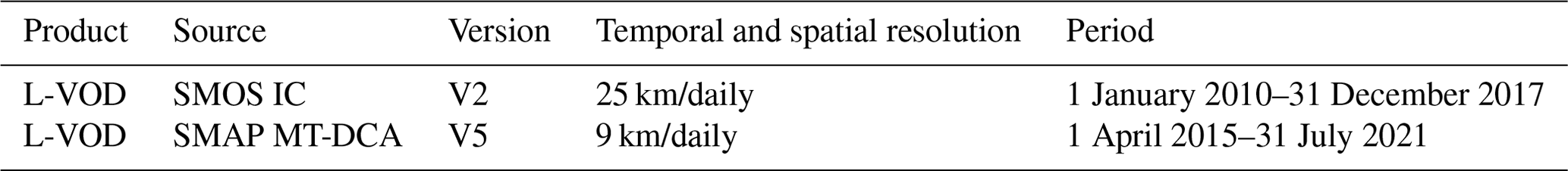
The SMOS IC L-VOD dataset is published by the European Space Agency (ESA) and has a satellite revisit period of 8 d, a spatial resolution of 25 km, and a global spatial coverage. This study uses the latest improved version 2 of L-VOD data for the period from 1 January 2010 to 31 December 2017, which does not require the use of the optical vegetation index as auxiliary data to drive the model, enhancing the independence and stability of the product. These data are derived from https://ib.remote-sensing.inrae.fr/index.php/smos-ic-v2-product-documentation/ (last access: 6 June 2024; Wigneron et al., 2021). Due to the long-term advantage of the SMOS L-VOD data, they are used as the low-spatial-resolution data for both the reference and target periods in the spatiotemporal fusion experiments. These data help in constructing the baseline data and generating the 9 km L-VOD data for the target moments.

The SMAP MT-DCA L-VOD dataset covers the global surface with a satellite revisit period of 3 d and a spatial resolution of 9 km. This study uses the latest SMAP MT-DCA version-5 L-VOD data released by Feldman and Entekhabi (2019), which update the data from 1 April 2015 to 31 July 2021. These data are derived from https://doi.org/10.5281/zenodo.5619583 (Feldman et al., 2021). The MT-DCA algorithm combines microwave radiometer data from the SMAP satellite and vegetation index data from MODIS while also considering the temporal autocorrelation of VOD. Similar to the SMOS IC algorithm, MT-DCA does not require optical auxiliary data to provide initial VOD values due to its consideration of VOD's temporal autocorrelation. SMAP L-VOD data have the advantage of high spatial resolution, which is used in this study as the high-resolution baseline data in the spatiotemporal fusion model to provide fine spatial detail information for the VOD fusion product. A specific description of the L-VOD data is given in Table 1.

Table 1 Description of the L-VOD data used in this study.

2.2 Auxiliary data

To carry out the relevant analysis more comprehensively and accurately, we use two important auxiliary datasets, i.e., land cover type data and Normalized Difference Vegetation Index (NDVI) data.

This study selected pixel points in different land cover types for accuracy validation. The data are based on the MODIS MCD12C1 V061 (Friedl and Sulla-Menashe, 2022), which provides global land cover types at annual intervals with a time span from 2001 to 2022 and a spatial resolution of 0.05° (approximately 5.6 km). This dataset uses multiple classification schemes, including the International Geosphere-Biosphere Programme (IGBP), the University of Maryland (UMD), and the Leaf Area Index (LAI) (Loveland et al., 1999; Hansen et al., 2000; Chen and Black, 1992). In this study, land cover data for 2017 and 2018 are used. The data are accessed and processed through the Google Earth Engine platform.

In this study, we choose long-term NDVI data to further evaluate the final product VOD_st. The data are based on the MODIS MYD13C1 V061 (Didan, 2021), which has a spatial resolution of 0.05° (approximately 5.6 km) and is synthesized over 16 d. This product provides a Vegetation Index (VI) value for each pixel, i.e., the Enhanced Vegetation Index (EVI) and the NDVI. We use the NDVI data from 2010 to 2021, which maintains continuity with the existing National Oceanic and Atmospheric Administration-Advanced Very High Resolution Radiometer (NOAA-AVHRR)-derived NDVI.

Considering the availability of the dataset, the study period for this research is from 1 January 2010 to 31 July 2021. For convenience, the original SMOS IC L-VOD product is referred to as VOD_smos, the original SMAP MT-DCA L-VOD product as VOD_smap, the gap-filling products as VOD_resmos and VOD_resmap, respectively, and the spatiotemporal fusion product as VOD_st.

3 Methodology

3.1 Data preprocessing

For the selected VOD_smos and VOD_smap datasets, preprocessing steps such as reprojection, anomaly handling, and resampling are required. Due to differences in the geographic coverage and projection methods of the SMOS and SMAP data products, reprojection is necessary. Additionally, considering that VOD typically ranges from 0 to 1.5, with higher values often observed in densely vegetated tropical regions, reaching up to approximately 1.2, there are occasional outliers exceeding 1.5 in specific areas like the Amazon and Congo river basins, accounting for approximately 1 % of the total (Fernandez-Moran et al., 2017; Li et al., 2022a). To minimize the potential accumulation of uncertainty in subsequent experiments caused by abnormal values, these data need to be removed. Furthermore, some regions may have negative VOD values due to unreliable retrieval caused by sensor limitations or land types such as permafrost or deserts. VOD values of less than 0 cannot be explained by physical properties. Following the guidelines of Wigneron et al. (2021) for the SMOS IC L-VOD data (https://ib.remote-sensing.inrae.fr/index.php/smos-ic-v2-product-documentation/, last access: 28 July 2024), negative VOD values will be set to 0 in this study to ensure result accuracy. Lastly, the low-resolution product VOD_smos will be preliminarily resampled to 9 km using nearest-neighbor interpolation to maintain consistency in the spatial resolution across all of the datasets. Our data utilize a global grid of 2000 × 4000 cells.

We consider that VOD has continuity over long temporal sequences but faces a significant proportion of spatial data gaps. Moreover, in the spatiotemporal fusion model, higher spatial coverage of input data, represented by a larger effective number N, leads to better spatiotemporal fusion effects. Therefore, our study initially proposes using a penalized least-square regression based on a three-dimensional discrete cosine transform (DCT–PLS) method to leverage spatiotemporal variation information to repair L-VOD data from the SMOS and SMAP satellites. Subsequently, seamless data will be input into a nonlocal filter-based spatiotemporal fusion model (STFM) to reconstruct historical 9 km data, aiming to maximize error reduction and enhance product quality.

3.2 Gap-filling

Given the significant spatial data gaps in the VOD_smos and VOD_smap datasets, and considering that frequency domain signal distribution is more concentrated and contains more comprehensive information, DCT is an effective algorithm for transforming signals into the frequency domain for computation (Wang et al., 2023). Additionally, PLS regression is a thin-plate spline smoothing method suitable for one-dimensional arrays and aims to balance data fidelity and the roughness of the mean function. Garcia (2010) demonstrated that DCT achieves PLS regression by expressing data as a sum of cosine functions oscillating at different frequencies. Due to the multidimensional characteristics of DCT, DCT-based PLS regression can be extended directly to multidimensional datasets (Wang et al., 2012). For large spatiotemporal datasets, utilizing spatiotemporal variation information to predict missing parts is highly effective. Furthermore, VOD data show significant temporal and spatial correlations, and DCT can capture this spatiotemporal correlation well. Therefore, this study uses the three-dimensional DCT–PLS method to fill the gaps in the global daily L-VOD data. The following section will briefly introduce the principles of the DCT–PLS algorithm for data repair.

Let x represent the spatiotemporal dataset with missing values. The solution formula for the filled data matrix y is as follows:

$$\begin{array}{}\text{(1)}& F\left(y\right)={∥Q^{\mathrm{1}/\mathrm{2}}\cdot (y-x)∥}^{\mathrm{2}}+\mathit{\lambda }∥{\mathrm{\nabla }}^{\mathrm{2}}y∥,\end{array}$$

where $\Vert \cdot \Vert$ denotes the Euclidean norm. Q is a binary matrix indicating the missing values in the original data, with the square root used for weight adjustment. ∇² is the Laplacian operator. λ is the smoothness factor, which measures the smoothness of the data y. The iterative solution for y can be transformed into the following formula:

$$\begin{array}{}\text{(2)}& y={\mathrm{DCT}}^{-\mathrm{1}}(G\cdot \mathrm{DCT}(Q\cdot (x-y)+y\left)\right).\end{array}$$

In this context, DCT is used to transform the data from the spatial domain to the frequency domain, where the data are then reconstructed. Finally, the inverse transform (DCT⁻¹) is applied to convert the reconstructed results back from the frequency domain to the spatial domain. G is a three-dimensional filtering tensor:

$$\begin{array}{}\text{(3)}& G_{(k_{\mathrm{1}},k_{\mathrm{2}},k_{\mathrm{3}})}={\displaystyle \frac{\mathrm{1}}{\mathrm{1}+\mathit{\lambda }{\left(\sum _{m=\mathrm{1}}^{\mathrm{3}}(\mathrm{2}-\cos \frac{(k_m-\mathrm{1})\mathit{\pi }}{N_m})\right)}^{\mathrm{2}}}},\end{array}$$

where k_m represents the kth element in the mth dimension (where $m=\mathrm{1},\mathrm{2},\mathrm{3}$), and N_m denotes the size of the data in the mth dimension of the matrix x.

In DCT–PLS modeling, the selection of the smoothing parameter λ is crucial. A higher value of the smoothing parameter will result in the loss of high-frequency components. To effectively fill the data gaps, λ should be as close to 0 as possible to minimize the smoothing effect. By calculating the normalized error between the original and reconstructed values, we can determine whether the model accurately captures the characteristics of the data. Thus, the smoothing parameter λ can be adjusted based on the error evaluation results to optimize model performance. The error ϵ is defined as follows:

$$\begin{array}{}\text{(4)}& \mathit{ϵ}={\displaystyle \frac{∥Q^{\mathrm{1}/\mathrm{2}}\cdot (y-x)∥}{∥Q^{\mathrm{1}/\mathrm{2}}\cdot x∥}}.\end{array}$$

3.3 Spatiotemporal fusion

Spatiotemporal fusion of remote sensing data is the process of integrating multisource remote sensing data into products that have spatiotemporal consistency and higher accuracy. Of these methods, both transformation-based and pixel-based reconstruction methods are commonly used approaches (Zhu et al., 2018; Belgiu and Stein, 2019). Transformation-based methods include techniques such as Fourier transform and wavelet transform (Fanelli et al., 2001; Gharbia et al., 2014). These methods fuse data by combining transform coefficients from different sources, offering simplicity and ease of implementation. However, they often suffer from lower accuracy and are prone to introducing noticeable artifacts into the fusion images. On the other hand, pixel-based reconstruction methods involve weighted averaging or other operations on pixel values from different source data to achieve fusion. This approach has become the mainstream method in current spatiotemporal fusion research due to its ability to preserve spatial details and improve overall accuracy. Within these methods, a spatial and temporal adaptive reflectance fusion model (STARFM) has been widely applied (Gao et al., 2006). An improved approach to the STARFM is used in this study.

This study aims to extend the SMAP 9 km VOD by developing a nonlocal filter-based STFM (Cheng et al., 2017). This model employs the transformation relationships between high-resolution spatial data and low-resolution temporal data over different time periods to effectively utilize the high spatiotemporal correlation in remote sensing image sequences and predict high-spatial-resolution data at the target time. For convenience, in this study, we refer to images with high spatial resolution and low temporal resolution as high-resolution images and conversely as low-resolution images, based on spatial resolution as the criterion.

As mentioned above, this experiment performs spatiotemporal fusion on the reconstructed data VOD_resmos and VOD_resmap to obtain the VOD_st product. Assuming that the changes in VOD are linear over a short period, the relationship between the data at different times t_k and t₀ within a pixel can be expressed as follows:

$$\begin{array}{}\text{(5)}& \begin{array}{rl}& \text{VOD\_resmos}(x,y,t_k)=\\ & a(x,y,\mathrm{\Delta }t)\cdot \text{VOD\_resmos}(x,y,t_{\mathrm{0}})+b(x,y,\mathrm{\Delta }t),\end{array}\end{array}$$

where (x,y) denotes a given pixel location in the low-resolution data, $\mathrm{\Delta }t=t_k-t_{\mathrm{0}}$, and a and b are the coefficients of the linear regression model describing the change in VOD_resmos between the two time points.

We assume that the high-resolution and low-resolution data obtained by different sensors in the same spectral band exhibit similar temporal variations. Thus, the linear relationship between low-resolution remote sensing images, as shown in Eq. (5), also applies to high-resolution remote sensing images. The high-resolution data at time t_k can be calculated as

$$\begin{array}{}\text{(6)}& \begin{array}{rl}& \text{VOD\_st}(x,y,t_k)=\\ & a(x,y,\mathrm{\Delta }t)\cdot \text{VOD\_resmap}(x,y,t_{\mathrm{0}})+b(x,y,\mathrm{\Delta }t).\end{array}\end{array}$$

It should be noted that the regression coefficients are derived locally and may vary with location. Hence, they cannot be applied globally. Additionally, the condition of the surface cover might undergo significant and complex changes during the prediction period. Therefore, the STFM algorithm incorporates a new nonlocal filtering method to minimize the impact of these factors on the fusion outcome.

The nonlocal filtering method seeks to make full use of the highly redundant information within the image, thus contributing to the estimation of the target pixel (Buades et al., 2005a, b; Su et al., 2012; Gilboa and Osher, 2009). Within the search window Ω, the similarity between the neighboring pixels and the central pixel will influence the determination of the weights. The weight calculation method is as follows:

$$\begin{array}{}\text{(7)}& W(x_i,y_i)={\displaystyle \frac{\mathrm{1}}{C(x,y)}}\cdot \exp \left\{-{\displaystyle \frac{\begin{array}{c}G\cdot \Vert \text{VOD\_resmos}\left(P\right(x_i,y_i\left)\right)\\ -\text{VOD\_resmos}\left(P\right(x,y\left)\right){\Vert }^{\mathrm{2}}\end{array}}{h^{\mathrm{2}}}}\right\},\end{array}$$

where C(x,y) is the normalization factor, G is the Gaussian kernel, and h is the filtering parameter. The term $(x_i,y_i)\in \mathrm{\Omega }$ represents the coordinates of neighboring pixels within the search window, and $P_{(x_i,y_i)}$ is the nonlocal similarity patch centered at (x_i,y_i). Once similar pixels are determined globally, their information is used to estimate the target pixel through weighted averaging. The final spatiotemporal fusion prediction model can be expressed as follows:

$$\begin{array}{}\text{(8)}& \begin{array}{rl}& \text{VOD\_st}(x_i,y_i,t_k)=\sum _{i=\mathrm{1}}^{n}W(x_i,y_i,t_{\mathrm{0}})\\ & \times \left[a\right(x_i,y_i,\mathrm{\Delta }t)\times \text{VOD\_resmap}(x_i,y_i,t_{\mathrm{0}})\\ & +b(x_i,y_i,\mathrm{\Delta }t)],\end{array}\end{array}$$

where n represents the number of similar pixels globally.

VOD_smos data are available from 1 January 2010 to the present, while VOD_smap data cover the period from 1 April 2015 to 31 July 2021. To fill the temporal blank in high-spatial-resolution L-VOD products before the launch of the SMAP satellite, we use 1 April 2015, the initial date provided by the VOD_smap product, as the time node. The time range to be predicted by the VOD_st product is defined as the T1 period, spanning the period from 1 January 2010 to 31 March 2015. To construct the baseline data required for the spatiotemporal fusion model, and considering the temporal correlation, we extend 1 year beyond the fusion input period, defining the T2 period as being from 1 April 2015 to 1 April 2016. To validate the quality of the fusion product VOD_st, we define the remaining period from 2 April 2016 to 31 December 2017 as the T3 period. For specific details, please refer to Fig. 1.

Figure 1 Spatiotemporal fusion experiment time segment division explanation.

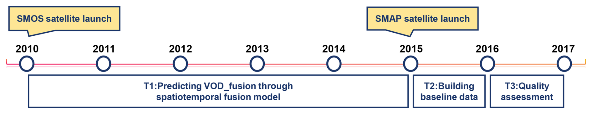
Figure 2 illustrates that the spatiotemporal fusion model requires paired high-resolution and low-resolution data to construct the baseline data. To achieve a more temporally correlated fusion product, we use the monthly averaged VOD_resmos and VOD_resmap from April 2015 to April 2016 to generate baseline data, which is a key step in learning the transformation relationships between high-resolution and low-resolution data across different periods. Subsequent experiments utilize these baseline data, inputting daily low-resolution VOD_resmos data for each corresponding month to obtain the daily high-resolution spatiotemporal fusion product VOD_st.

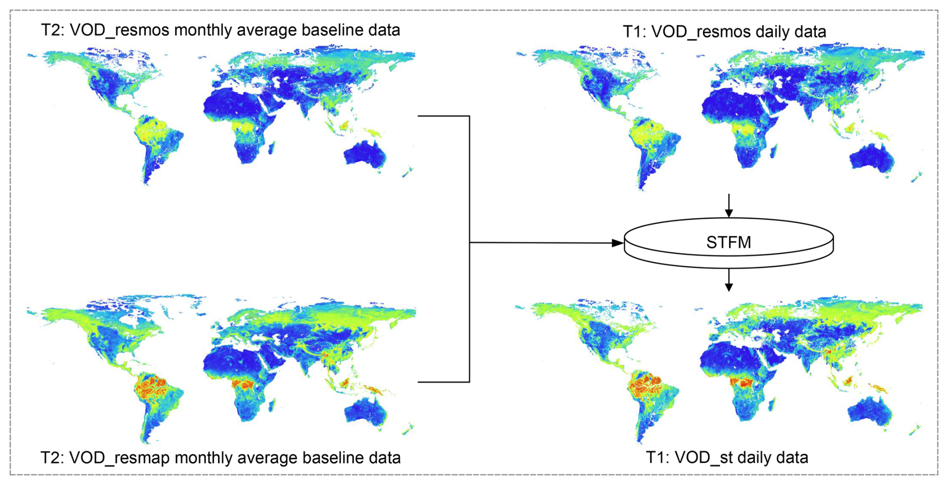
Figure 2 The spatiotemporal fusion process.

In summary, this study first utilizes the DCT–PLS method to fill gaps in the original missing data, obtaining the reconstructed products (VOD_resmos and VOD_resmap). Subsequently, the reconstructed global seamless daily data are input into the STFM, generating the 9 km VOD_st product for unreleased periods of the SMAP satellite. The main experimental process is illustrated in Fig. 3. The accuracy validation part is detailed in Sect. 4.

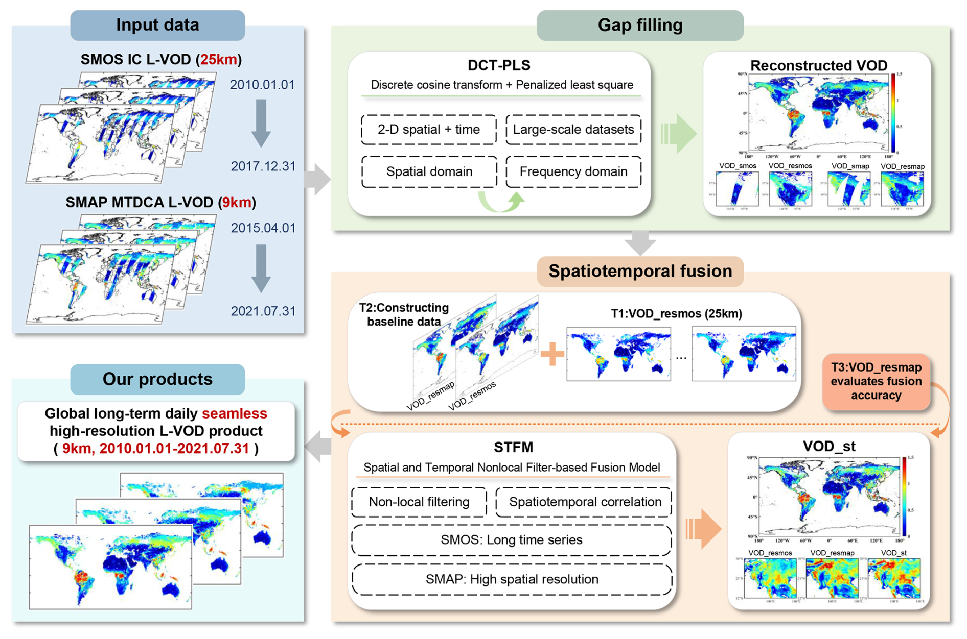
Figure 3 General flowchart of the experiment.

3.4 Experimental setup

In this study, a three-dimensional dataset is constructed with a monthly time series length. The DCT–PLS method is an iterative algorithm designed to fill missing values in multidimensional data. In this experiment, the number of iterations is set to 100, with the initial prediction of the original data made using the nearest-neighbor interpolation method. The smoothing parameter (λ) follows a logarithmic sequence from 10⁻³ to 10⁻⁶. During the imputation process, the algorithm gradually reduces the smoothing parameter to achieve a transition from coarse to fine imputation.

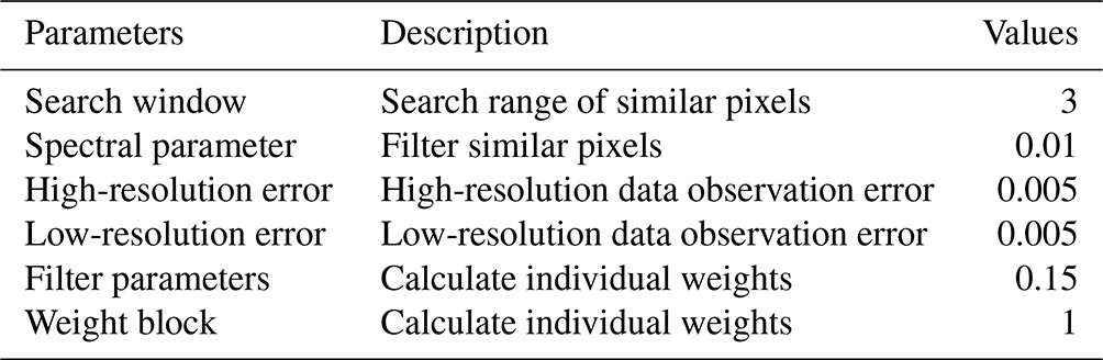
The STFM algorithm processes data in batches, using the high-resolution and low-resolution monthly average baseline data constructed for the T2 period, along with the daily low-resolution data for the corresponding month at the target time. After multiple adjustments, the optimal combination of parameters for the L-VOD data is determined. Table 2 describes the meaning and specific values of these parameters.

Table 2 Parameterization of the STFM algorithm in this study.

The quantitative evaluation metrics used in the experimental section of this study include five indicators: the correlation coefficient (R), the coefficient of determination (R²), the root mean square error (RMSE), the bias, and the mean absolute error (MAE).

4 Experiment results and discussions

4.1 Gap-filling

4.1.1 Reconstructed results

The gap-filling results for 1 June 2016 are illustrated in Fig. 4. We observe that the reconstructed results not only retain the existing values of the original data but also reasonably fill in the missing parts. The filled areas show no obvious discontinuities or gaps in the surrounding data. Additionally, the reconstruction results maintain the details of the original image, such as topographic features and boundaries.

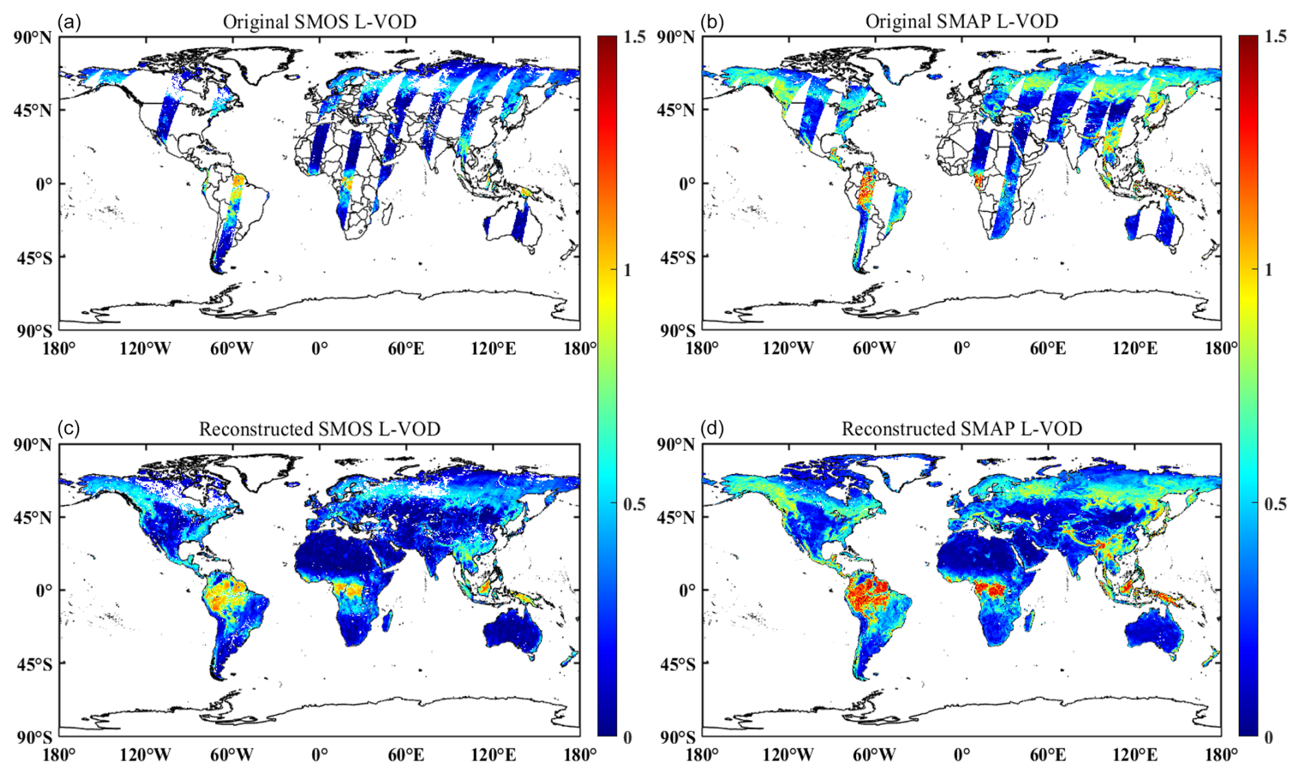
Figure 4 Comparison results of SMOS (a, c) and SMAP (b, d) L-VOD before and after reconstruction on 1 June 2016.

To investigate the detail recovery capability of the DCT–PLS model further, Fig. 5 presents the comparison results of the magnified data in a local area. It can be seen that, whether in high-value or low-value situations, the reconstruction results still exhibit reasonable spatial variations in the missing areas, without clear boundaries.

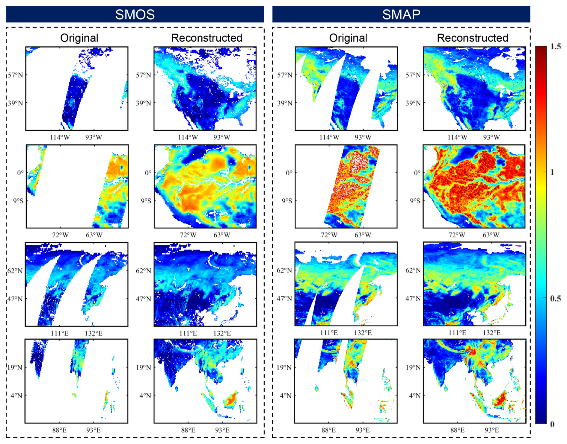
Figure 5 Four localized regions are selected to compare the reconstruction effects of SMOS and SMAP in the same localized region on 1 June 2016.

4.1.2 Time series validation

Apart from maintaining spatial continuity as described in Sect. 4.1.1, temporal consistency is crucial for the reconstructed L-VOD products. In this section, we analyze the time series of representative pixels with different missing proportions and different land surface types before and after reconstruction.

Take the SMAP L-VOD data in 2018 as an example. In Fig. 6, we show three time series with varying proportions of data gaps and their corresponding model outputs. The three pixel points are from western Canada (52.155° N, 64.755° W), southern Russia (55.215° N, 95.355° E), and the northeastern Democratic Republic of the Congo (1.215° N, 26.325° E). In Fig. 6, the red line represents the original values, overlaid on the blue line representing the reconstructed values. In other words, the DCT–PLS model does not alter the original pixel values themselves, preserving the original characteristics of the data and maintaining continuity in the reconstructed results. Notably, the boxes in Fig. 6 indicate that the model effectively captures the extreme values present in the original dataset. These findings suggest that the DCT–PLS model used in this study reliably predicts the missing portions.

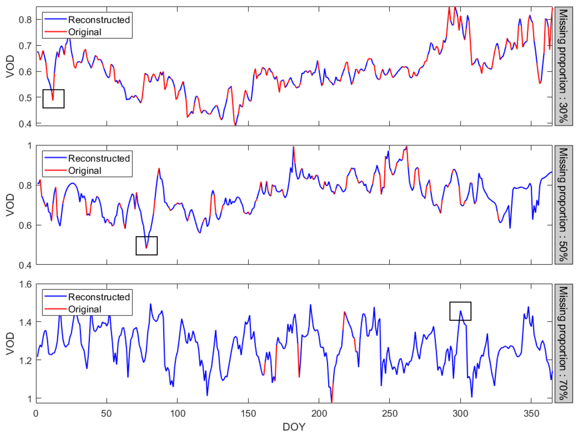
Figure 6 Results of the temporal variation in selected pixels of different missing-data ratios in 2018, with red representing original values, blue representing model-reconstructed values, and rectangles representing some extreme value reconstruction results.

Combining Sentinel-2 satellite imagery with MODIS MCD12C1 V061 land cover classification data, Fig. 7 shows the temporal variation results across different land cover types. Four land types are selected for study: forest, shrubland, cropland, and grassland. To ensure consistency, we select pixels with 52 % missing data throughout the year for analysis. The time series illustrates the seasonal variations in the different land types. For instance, forests and grasslands exhibit significant vegetation changes during certain seasons, such as periods of vigorous growth and dormancy. Croplands show distinct cyclic fluctuations in VOD, reflecting the planting and harvesting cycles of crops. Typically, VOD is lower during the sowing season, peaks during the growth period, and decreases again after harvest.

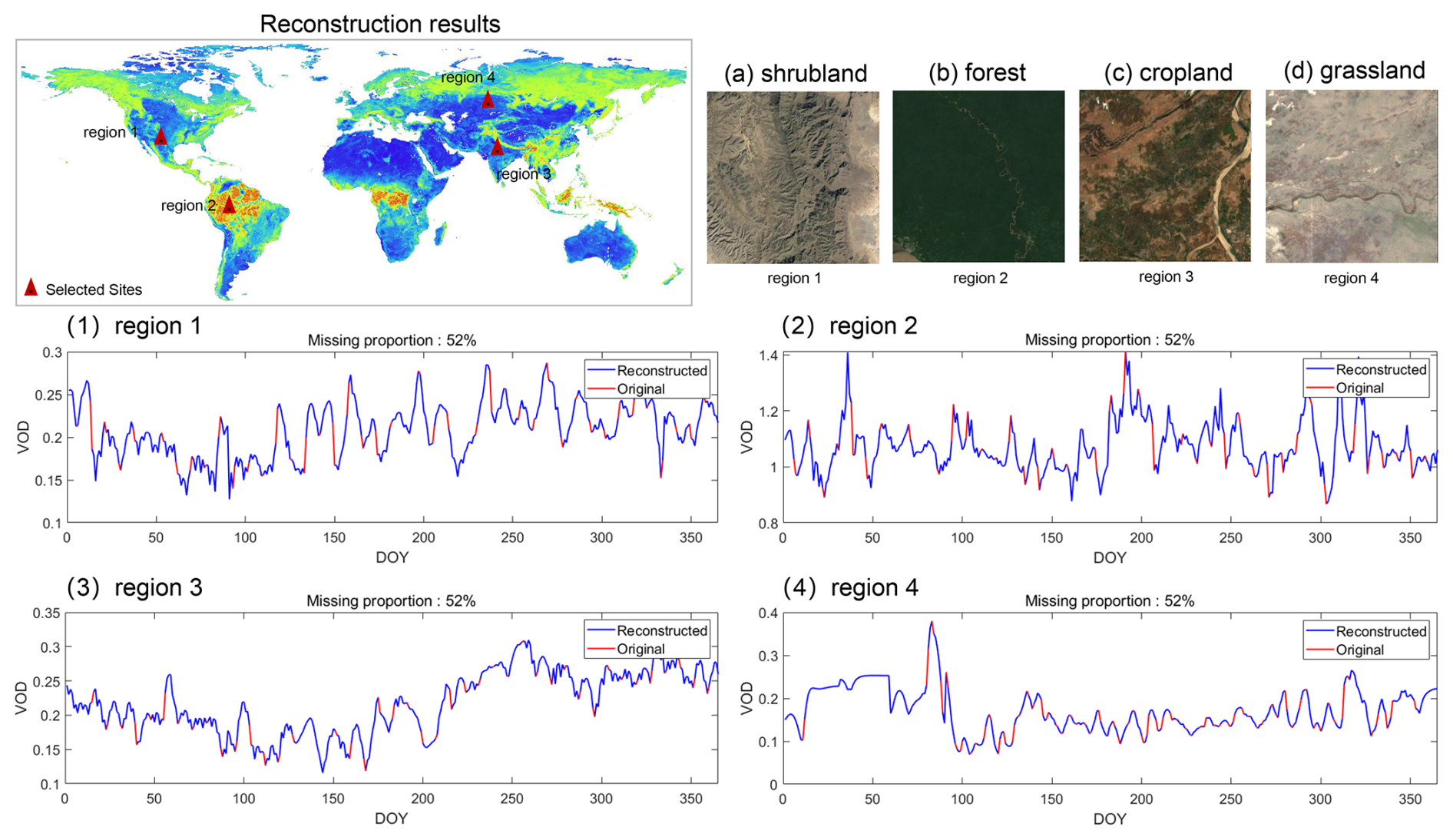
Figure 7 The red dots in the figure indicate the pixel points selected to characterize the temporal variation of L-VOD under different vegetation conditions. Four different surface types are selected here, i.e., (a) scrub, (b) forest, (c) cropland, and (d) grassland. Panels (1)–(4) are the time series variation maps of the corresponding pixels under the above surface types.

4.1.3 Simulated missing-region validation

To quantitatively analyze the performance of the DCT–PLS method in spatiotemporal data reconstruction, we design a series of experiments. Considering the current lack of site data for L-VOD products, we simulate missing data by removing original values.

Taking the original SMAP L-VOD data from 20 July 2020 as an example, we create four simulated square missing areas (80 × 80 pixel) in North America, South America, Africa, and Asia, as shown in Fig. 8. This allows us to easily compare the reconstructed VOD areas with the original VOD areas to validate the spatial continuity of the gap-filling products. Figure 8a and b, respectively, depict the original and reconstructed results of the simulated missing areas on 20 July 2020. It can be seen that the output data are continuous within the original valid areas. In the simulated missing patches, the spatial texture information is also continuous, without noticeable boundary reconstruction effects.

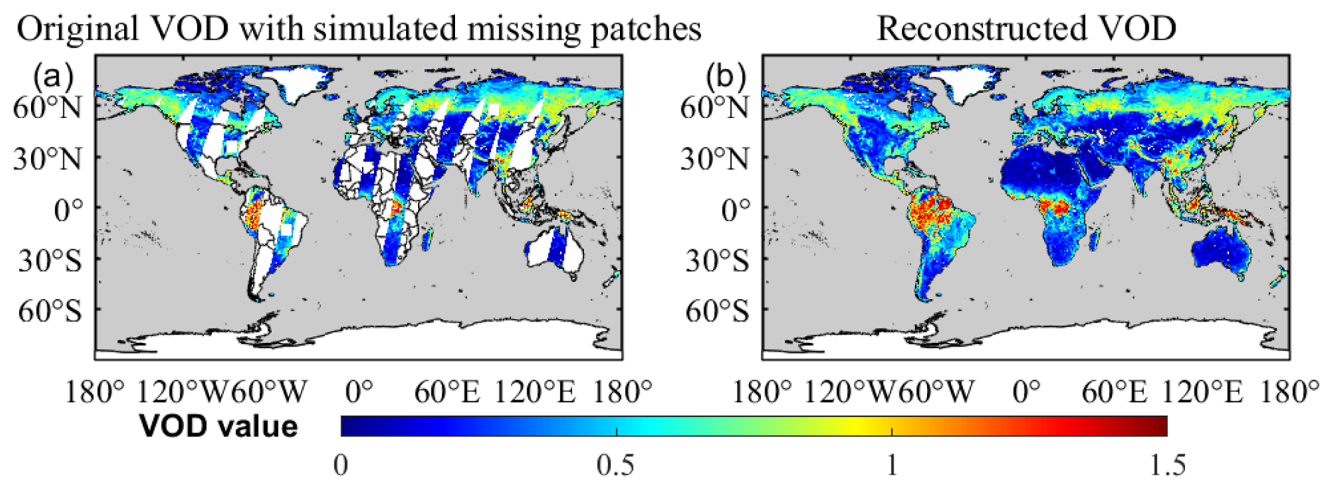
Figure 8 Original and reconstructed results with simulated missing regions on 20 July 2020: (a) original data with four simulated missing patches and (b) reconstructed data. The gray background represents the ocean.

To better analyze the spatial details of the reconstructed VOD data, we magnify the results of the four simulated regions in Fig. 8. Figure 9 shows the detailed original and reconstructed spatial information for the four simulated patches on 20 July 2020. It can be clearly seen that the reconstructed patches have high consistency with the original patches.

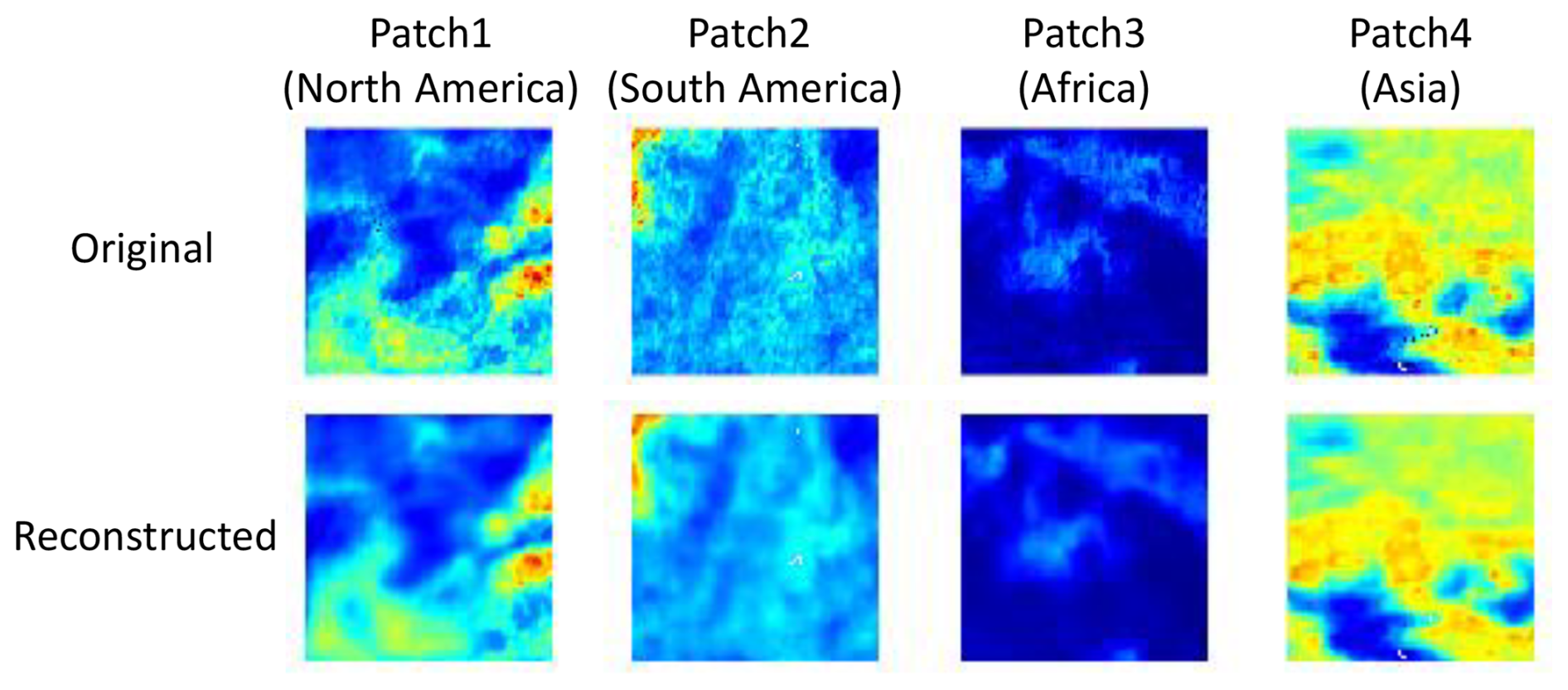
Figure 9 Detailed original and reconstructed spatial information of the four simulated missing patches. The four simulated missing patches (80 × 80 pixels) are from the original SMAP L-VOD data from 20 July 2020 taken from North America, South America, Africa, and Asia.

Figure 10 shows scatterplots of the original and reconstructed data for the four simulated regions mentioned above. The results indicate that the VOD in the simulated missing areas has a high reconstruction accuracy, with R² values ranging from 0.883 to 0.978. The RMSE does not exceed 0.05, and the MAE does not exceed 0.04.

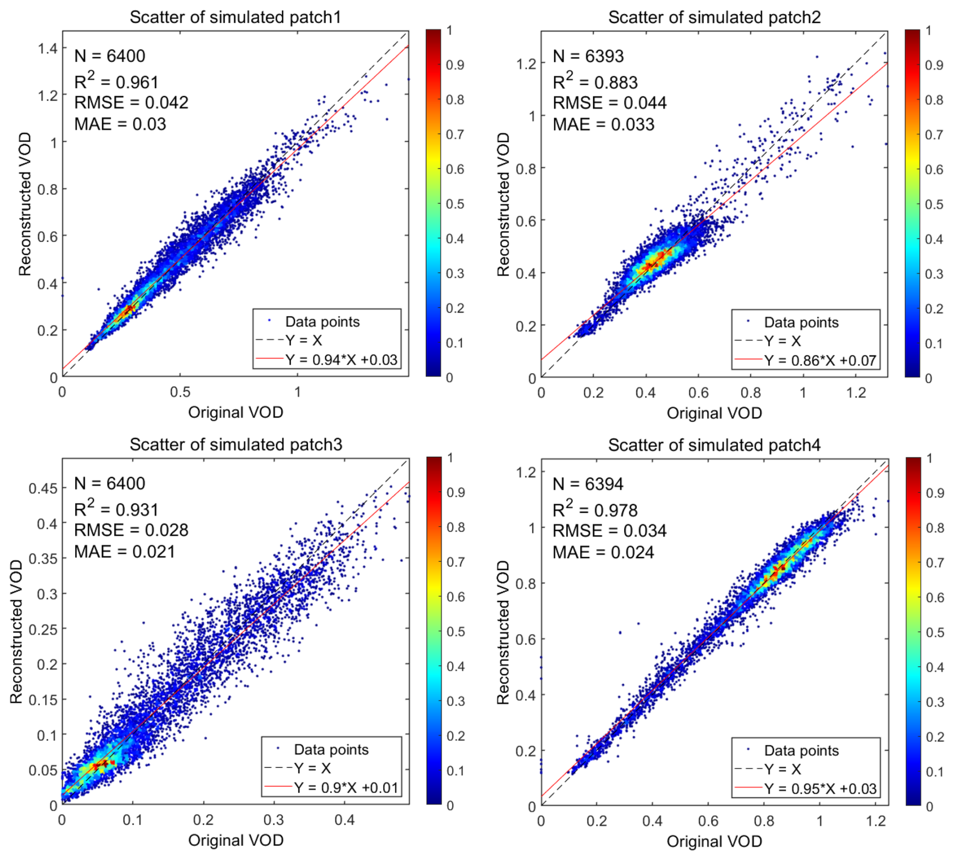
Figure 10 Scatterplots of the original and reconstructed data for the four simulated missing regions on 20 July 2020. The colors and the color bar indicate the density of the data points in the scatterplot.

Additionally, to better simulate the missing patterns of the original data and make the validation results more realistic, we create missing data by applying real missing masks from the original data, as shown in Fig. 11. This method randomly applies the missing mask from one day to data from other days, avoiding the influence of fixed missing-data patterns on the validation results. It is suitable for time series data and can simulate missing-data patterns at different time points. The DCT–PLS method is then used to reconstruct the missing data, with the original values serving as the reference to compare the accuracy of the reconstruction.

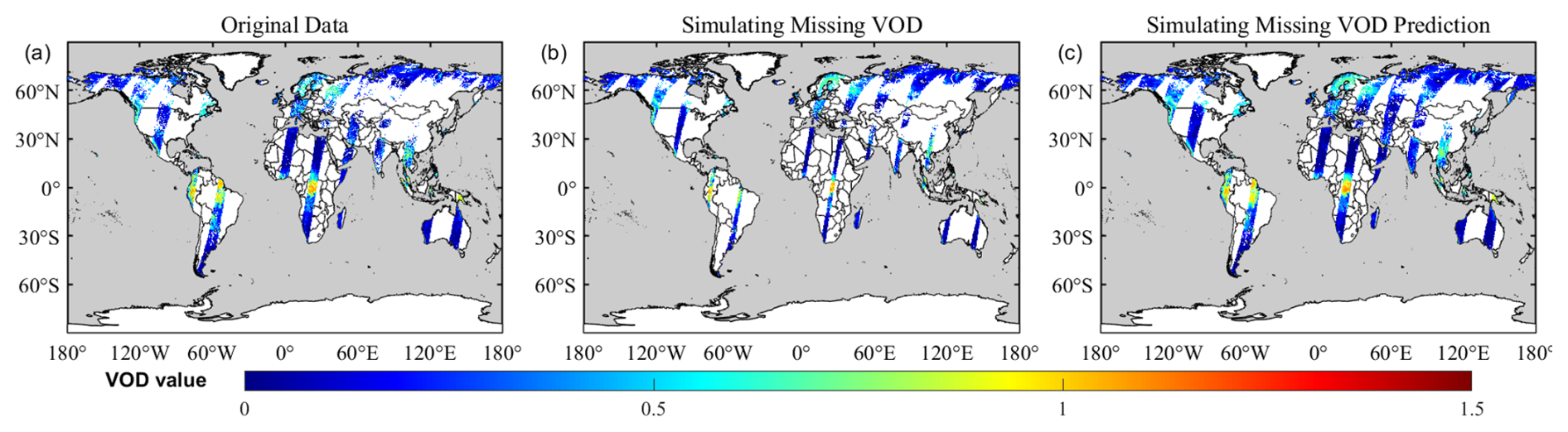
Figure 11 Simulation of real missing data on 9 September 2011: (a) original striped data, (b) simulated real missing mask data, and (c) the reconstructed result for the missing parts.

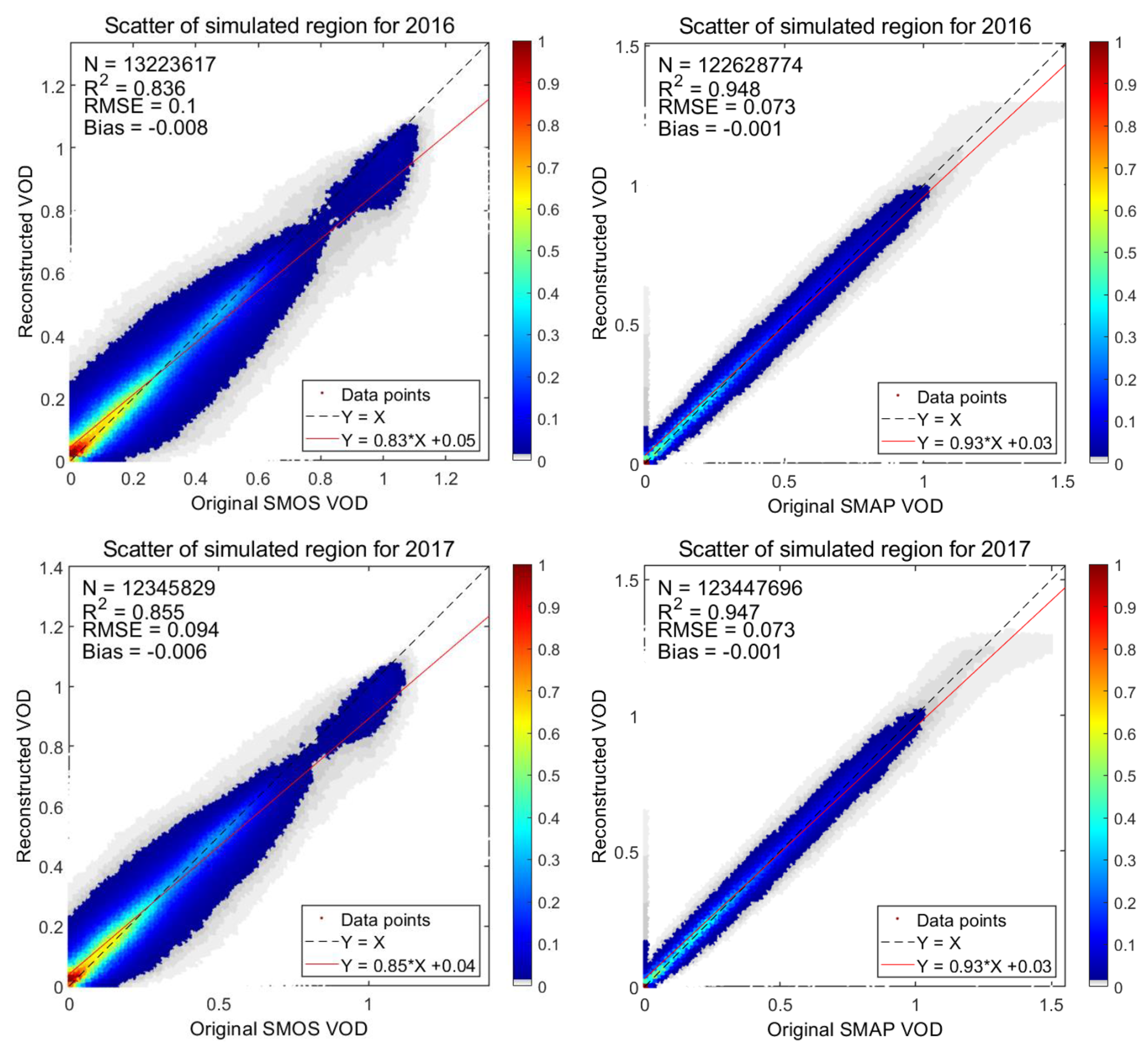
By simulating real missing masks, we validate the effectiveness of the DCT–PLS reconstruction method. We analyze the overlapping period of SMOS and SMAP data, and Fig. 12 shows the results of missing-value reconstruction for the SMOS and SMAP L-VOD datasets for 2016 and 2017. The results indicate that the proposed method performs excellently in reconstructing missing values. Specifically, for the SMOS L-VOD data, the R² exceeds 0.8, the RMSE is less than 0.1, and the biases are only −0.008 and −0.006, respectively. The SMAP L-VOD data, likely due to their more complete original data distribution and smaller proportion of missing values, show even better reconstruction results, with an R² of 0.948 and an RMSE of 0.073. These metrics indicate a high degree of consistency between the predicted and original values, with minimal errors and no significant systematic bias.

Figure 12 Scatterplots of the accuracy for the simulated missing parts, i.e., the accuracy assessment results for Fig. 11a and c. Here, we take the overlapping period of SMOS and SMAP in 2016 and 2017 as examples.

4.2 Spatiotemporal fusion

4.2.1 Comparison of VOD_st and VOD_resmap values in the overlapping period

This experiment aims to use a spatiotemporal fusion model to generate 9 km L-VOD products, making the fusion product (VOD_st) an effective substitute for the high-resolution VOD_resmap product before its release. The closer the values of VOD_st are to those of VOD_resmap, the higher the quality of the fusion product. We first validate the accuracy of VOD_st by comparing it with VOD_resmap in the T3 period. Figure 13 shows boxplots that integrate the daily accuracy assessment results on a monthly basis. Three different metrics (R², RMSE, and bias) evaluate the differences between VOD_st and VOD_resmap. Overall, R² remains between 0.88 and 0.96, indicating a high correlation between the fusion product and the 9 km product. Notably, the accuracy is highest during the summer due to the largest spatial coverage, resulting in more valid data input into the spatiotemporal fusion model.

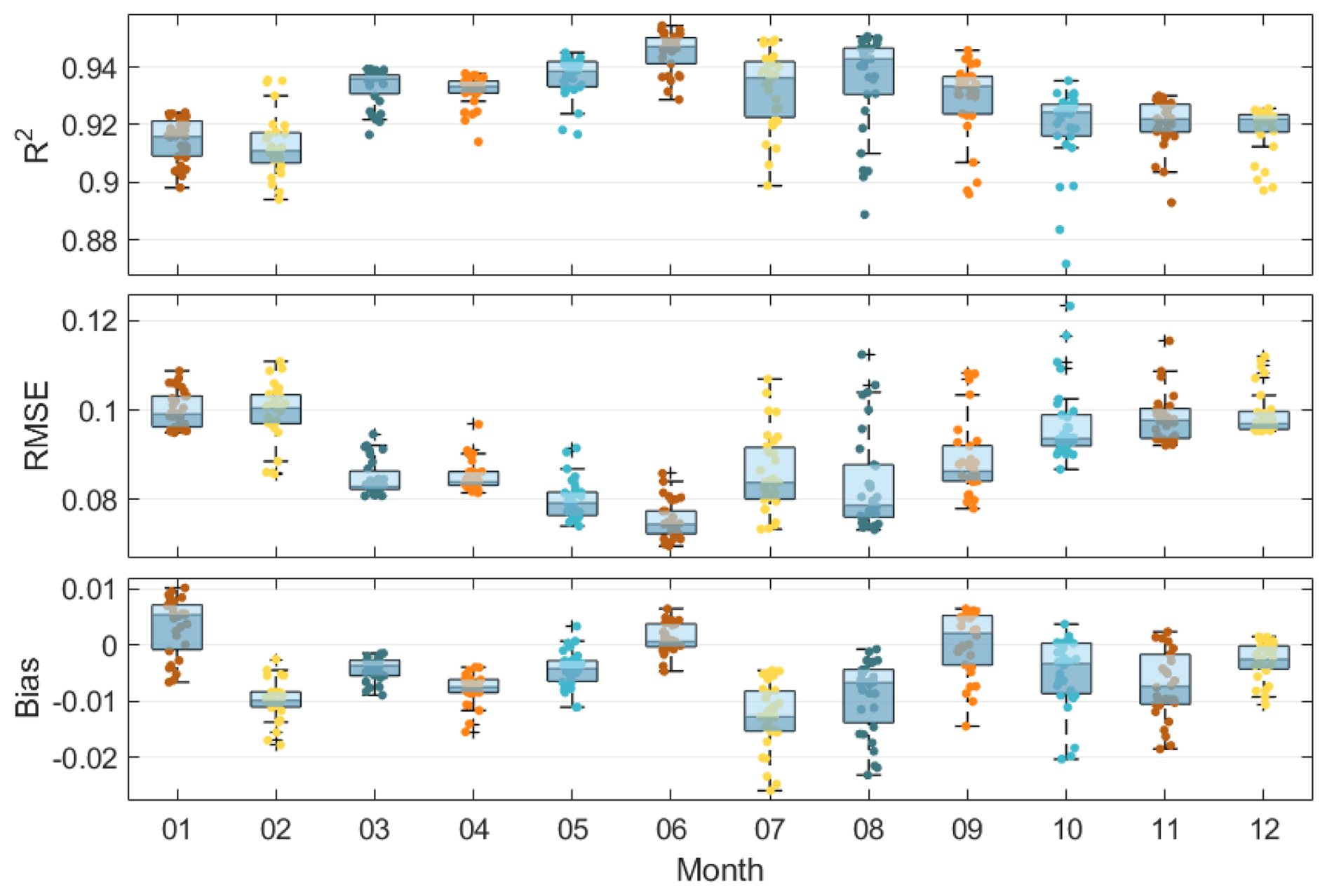
Figure 13 Boxplots of R², RMSE, and bias for VOD_resmap and VOD_st during the T3 period. The x axis represents the months, and each box represents the accuracy metrics for all of the days in the current month. The shading of the boxes is divided by the median line.

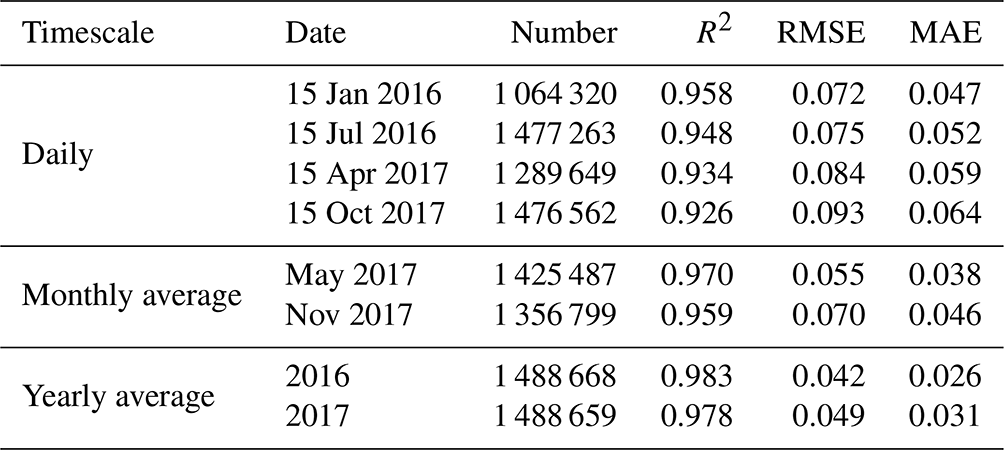
This experiment also conducts multiple validations on three different timescales: daily, monthly, and yearly. Table 3 presents representative evaluation results. The accuracy assessment covers these three timescales and the four seasons, which essentially represents the quality of the fusion product. We observe that the results during the T2 period show higher accuracy, which can be attributed to the baseline data used in constructing the spatiotemporal fusion model being sourced from the T2 period. Furthermore, the accuracy is highest on a global scale, aligning with the principle of the spatiotemporal fusion model that the fusion effect improves with higher spatial coverage, i.e., a larger effective number (N). Overall, R² consistently remains above 0.8, RMSE around 0.1, and MAE below 0.1, indicating a high correlation between VOD_st and VOD_resmap in terms of values.

Table 3 Evaluation results of VOD_resmap and VOD_st at three timescales.

Considering that the input data of the fusion model are reconstructed, some errors may be introduced. The original daily data are closest to the real situation, so comparing them with the fusion result can verify the authenticity and reliability of the fusion results. Figure 14 shows the scatter density plot between the fusion product VOD_st and the original 9 km data VOD_smap, allowing us to more intuitively visualize the excellent correlation between the two.

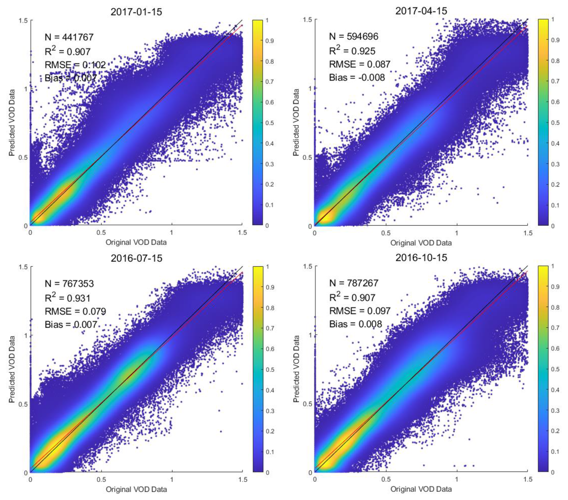
Figure 14 Scatter density plot between VOD_st and VOD_smap, selected from mid-season data for the corresponding season during the T3 period.

Despite the large number of data in the model (N ≥ 441 767), the results indicate that the fusion product and the original data still achieve excellent convergence, maintaining a high degree of linear correlation. There is a clear tendency for the fusion results to underestimate higher values and overestimate lower ones. This might be due to the original data handling of outliers (negative values and values greater than 1.5). Additionally, the weight distribution during the fusion process may lead to data smoothing, reducing data volatility and thus weakening extreme values. However, in the high-value range of 1–1.5, VOD_st shows partial underestimation, which is considered a positive phenomenon in this study. The VOD_smos and VOD_smap products use different algorithms and have differences in their data ranges. It is believed that VOD_smap tends to overestimate data in the high-value range. The fusion product obtained through the spatiotemporal fusion process is closer to VOD_smos in this range, effectively complementing the two products.

Through comprehensive accuracy assessment of the fusion data, we easily observe that the fusion data not only maximally align with the characteristics of the original observational data but also maintain consistency with the reconstructed data in the missing regions.

4.2.2 Long-term comparison

Since the input data for the spatiotemporal fusion model are low-resolution VOD products from the T1 period, we expect the fusion product to not only maintain high numerical consistency with VOD_resmap but also show a synchronized temporal trend with VOD_resmos. We compute the monthly averages of effective pixels for VOD_resmos, VOD_resmap, and VOD_st from 2010 to 2017, analyzing their temporal variations, as shown in Fig. 15. The results indicate that, from 2010 to 2017, VOD_st shows a generally synchronized trend with VOD_resmos, demonstrating effective learning of the temporal characteristics of the SMOS satellite product. The temporal trend lines of VOD_st and VOD_resmap generally align, with VOD_st values falling between the original data, indicating that it has effectively captured the numerical characteristics of both the SMOS and SMAP satellites, making it a suitable complement for VOD_resmap during missing periods.

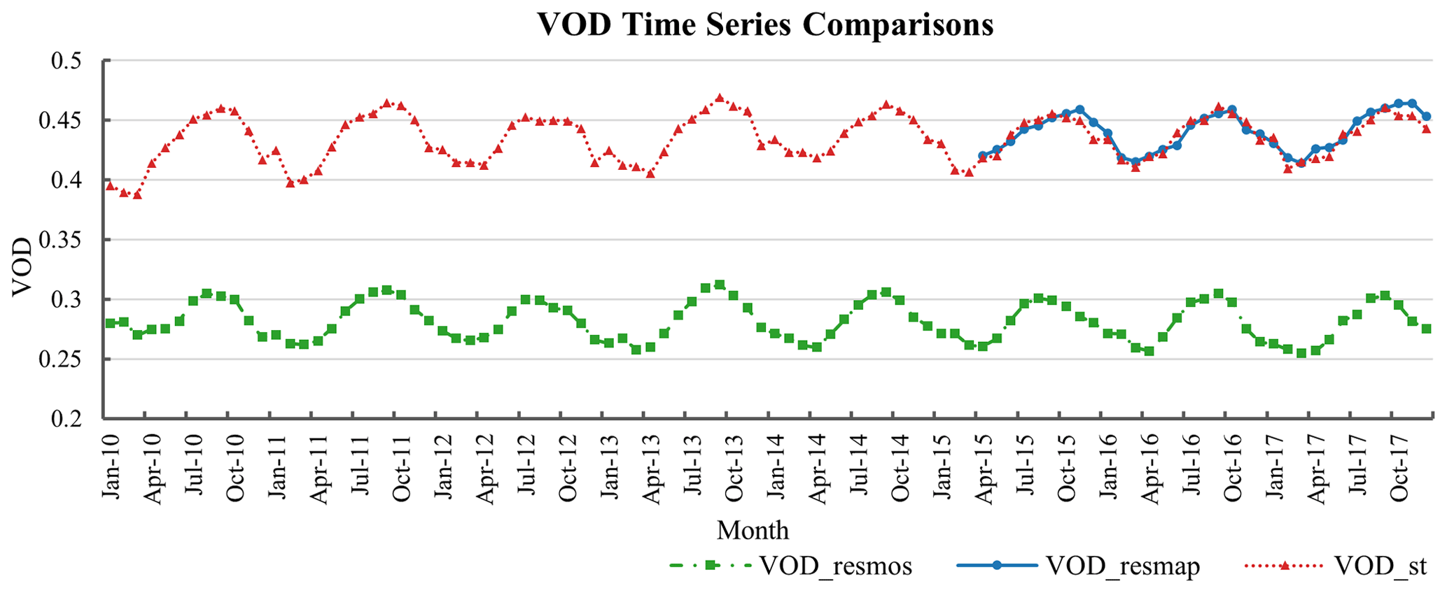
Figure 15 Temporal variation of monthly averages of valid VOD_resmos, VOD_resmap, and VOD_st pixels from 2010 to 2017. Green represents VOD_resmos, blue represents VOD_resmap, and red represents VOD_st.

4.2.3 Spatial distribution comparison

After analyzing the temporal characteristics of the three products, it is also necessary to discuss the spatial distribution of VOD_st. In this experiment, VOD_resmos and VOD_st from the T1 period in 2011 are selected for spatial distribution comparison to represent the mid-season L-VOD products, demonstrating spatial distribution changes across the different seasons. As shown in Fig. 16, corresponding to the conclusion that VOD_st numerically exceeds VOD_resmos, it can be observed that VOD_st and VOD_resmos exhibit similar spatial distribution patterns across the different seasons. With the warming of spring, vegetation begins to grow, especially in the polar regions where snow and ice melt, expanding the spatial coverage of VOD. As temperatures rise in summer and fall, the coverage area of VOD increases and VOD values rise significantly, which is particularly noticeable in summer. The consistency in the spatial distribution changes once again demonstrates the reliability of the spatiotemporal fusion results.

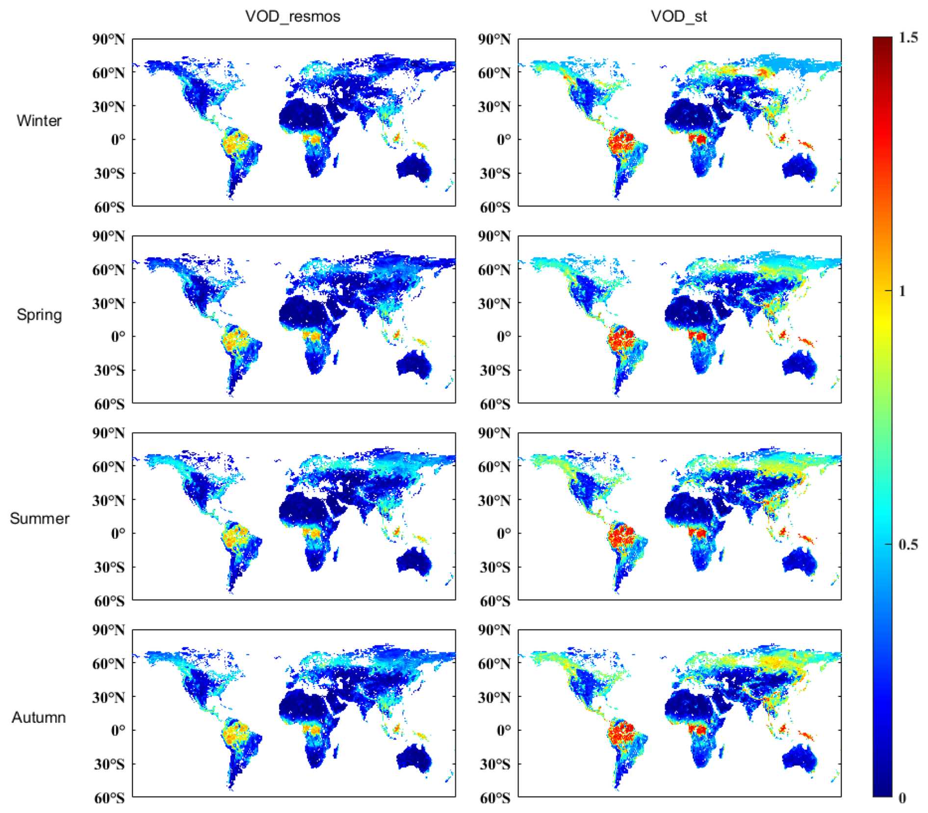
Figure 16 Comparison of the spatial distribution between VOD_resmos and VOD_st, using mid-season data from 2011 for the respective seasons.

4.2.4 Comparison of spatial details

To visually compare the spatiotemporal fusion results, Fig. 17 selects the mid-summer season of 2017 for a comparison of the three products. Due to the lack of 9 km L-VOD data from 2010 to 2015, we use VOD_resmos from this period to correct the spatiotemporal fusion results. Therefore, VOD_st maintains consistent spatial coverage with VOD_resmos. Additionally, because the spatiotemporal fusion model incorporates the characteristics of the VOD_resmap baseline data, it can be observed that VOD_st improves the underestimation seen in the original SMOS satellite product.

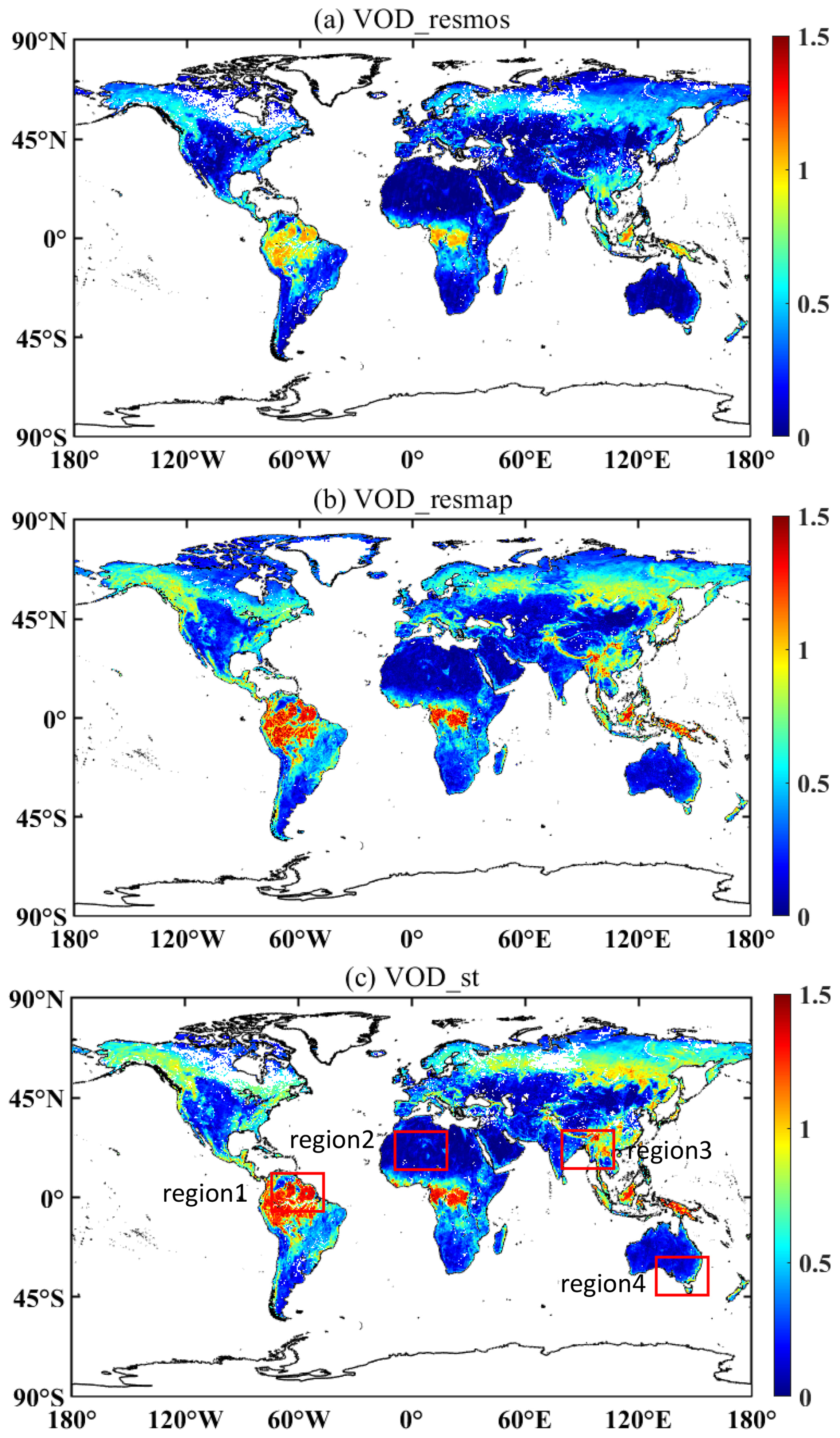
Figure 17 To visually compare the spatiotemporal fusion results, we select the mid-summer season of 2017 to compare the model inputs and outputs: (a) VOD_resmos, (b) VOD_resmap, and (c) VOD_st. Based on the MODIS MCD12C1 V061 data, the red boxes in panel (c) are the four representative regions.

We expect the VOD fusion product (VOD_st) to capture detailed information comparable to the spatial resolution of the 9 km L-VOD product from the SMAP satellite. Therefore, we further analyze the spatial detail representation capability of VOD_st. During the T1 period, only the coarse-resolution VOD_resmos and VOD_st are available, and during the T2 period, VOD_resmos and VOD_resmap contribute to the spatiotemporal fusion baseline data. Hence, in this experiment, we select the mid-summer season of the T3 period to compare VOD_resmos, VOD_resmap, and VOD_st, evaluating the spatial detail quality of the fusion product. Based on the MODIS MCD12C1 V061 land cover category data, we choose four representative regions, as indicated by the red boxes in Fig. 17c.

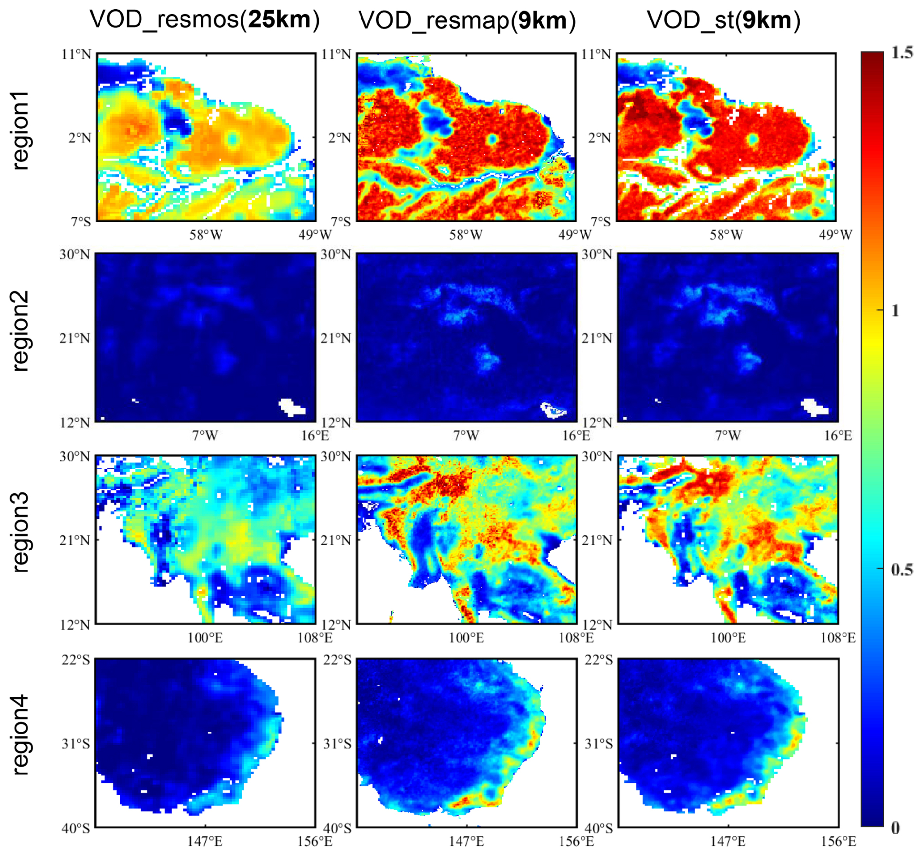
Figure 18 VOD_resmos, VOD_resmap, and VOD_st in the summer season of the T3 period are selected for comparison to evaluate the quality of the spatial details of the fusion products. Based on the MODIS MCD12C1 V061 land cover category data, four representative regions are selected, as indicated by the red boxes in Fig. 17c.

Figure 18 compares the spatial details of three L-VOD products. We find that the spatial details of VOD_st are significantly better than VOD_resmos and very close to VOD_resmap. This is because VOD_st effectively learns the characteristics of the VOD_resmap baseline data through the spatiotemporal fusion model, adequately considering the spatiotemporal correlations of VOD in the neighborhood. For example, it captures patchy features in region 2 and high-value boundary areas in region 4. Compared to VOD_resmap, VOD_st exhibits some gaps, primarily due to missing information from the original coarse-resolution VOD_resmos dataset.

5 Discussion

5.1 Comparisons with time series averaging

Currently, there is a lack of seamless daily L-VOD data. Therefore, we attempt to synthesize monthly averages of VOD_resmos and VOD_resmap data for a comprehensive comparison. Taking July 2015 data as an example, we consider the monthly average of the original strip data to be the benchmark for qualitative analysis of the corresponding reconstructed results.

Figure 19 compares the overall and local monthly average data before and after reconstruction. We believe that the daily variations in L-VOD values are not significant. Consequently, whether the missing data are filled or not, the overall spatial coverage remains largely consistent, without noticeable blocky patterns. We select a relatively representative area, Kalimantan (5° S–8° N, 108–120° E). The VOD signals on Kalimantan are higher, and the missing-data proportion mainly ranges from 50 % to 80 %, which can better reflect the reconstruction ability. Kalimantan is characterized by a large area and diverse tropical rainforests. Located in the tropical climate zone, it has complex climatic conditions, abundant precipitation, and extreme weather events that can impact vegetation. With diverse landforms and a special geographical location as well as social and economic activities such as agricultural development and ecotourism, this island has become a typical area for testing the effectiveness and reliability of the reconstruction method in complex environments. In local areas, the monthly average data after reconstruction are smoother, almost without the striped distribution phenomenon.

Figure 20 compares more representative regions. For SMOS data, the original data in certain regions (such as region1 and region2) show significant stripe-like gaps or discontinuities. These issues are resolved well in the reconstructed data, resulting in smoother and more continuous data. For SMAP data, the original data in region2 show significant missing blocks (white areas), where the nearby data may have large monthly average changes due to numerous missing days. The filled data effectively improve this situation, appearing more complete and smooth overall compared to the original data. Overall, in all three regions, the reconstructed data show significantly better performance in local areas, eliminating the striped distribution caused by missing original data and demonstrating a more uniform spatial distribution.

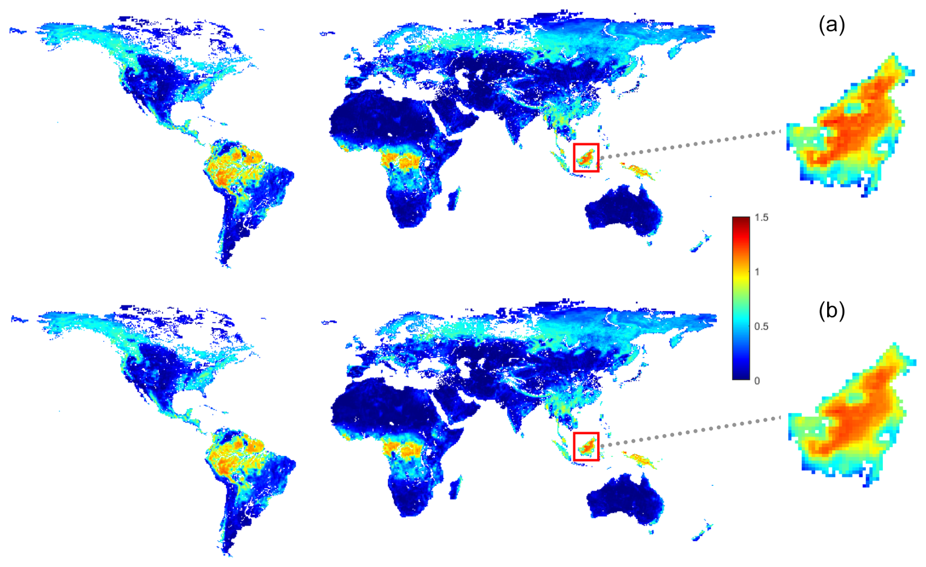
Figure 19 Original (a) and reconstructed (b) results for the July 2015 SMOS VOD monthly average. At a global scale, the overall coverage remains consistent. The red boxes highlight local areas, indicating that the monthly average spatial variations in the reconstructed data are smoother and free of striping.

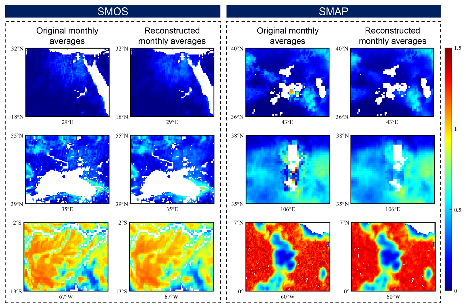
Figure 20 Here three regions are selected for each type of satellite product to compare the monthly average results of the original and reconstructed data under different factors.

5.2 Evaluating VOD against a vegetation-related parameter

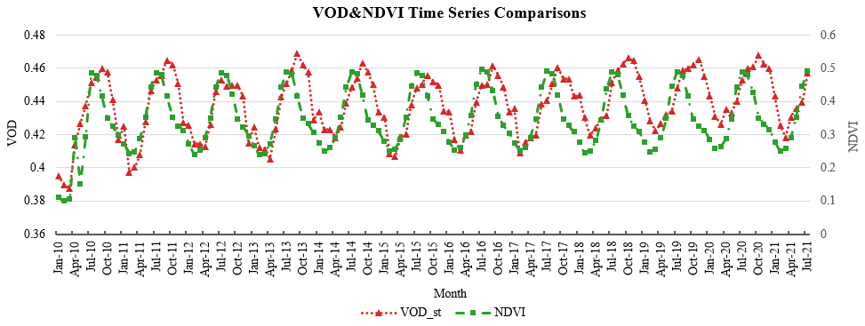
To enhance clarity, we evaluate VOD against the vegetation-related parameter NDVI. The results of the monthly average comparison between VOD_st and NDVI are shown in Fig. 21. We can observe that the seasonal trends of VOD_st and NDVI are highly consistent, showing obvious periodic characteristics. During the summer months corresponding to the period of maximum vegetation growth and leaf production, the values of these parameters increase significantly, and they decline as the vegetation ages. This consistency indicates that VOD_st can effectively capture the changes in vegetation growth, similar to traditional optically based indices like NDVI. Notably, VOD_st exhibits a slight lag in its seasonal changes compared to NDVI, but this lag is not due to the quality of VOD_st. Our findings are in line with previous studies (Lawrence et al., 2014; Li et al., 2021), which also reported that VOD data have a slight lag when compared with optical vegetation indices.

Figure 21 Long-term monthly average trend comparison between VOD and NDVI.

5.3 The bias between the SMOS and SMAP products

SMOS and SMAP sensors have different observational capabilities, and the differences in instrumentation result in different ways of sensing and measuring VOD. In addition, the two have different VOD retrieval algorithms, which can also cause bias. The bias between the SMOS and SMAP VOD products may introduce errors during the data fusion process, thereby affecting the accuracy and reliability of the fused product (Li et al., 2022b).

In the context of our study, we focus on the overall temporal and spatial trends of VOD rather than eliminating the bias between the two sensors' products. This is based on the assumption that, within the same spectral band, high-resolution and low-resolution data obtained from different sensors have similar temporal changes. We believe that these similar temporal variations can still provide valuable information for our research objectives. For instance, when analyzing the long-term trends of vegetation dynamics or the response of vegetation to environmental changes, the common temporal patterns in SMOS and SMAP VOD data can be used to draw meaningful conclusions. In addition, our study is more concerned with the general performance and usability of the fused product. We believe that the bias does not significantly distort the overall patterns and relationships.

We understand the importance of the bias issue and acknowledge that it may be necessary to further explore ways of mitigating bias in future studies for more accurate and refined results. However, in the scope of this current study, our approach based on the assumption of similar temporal variations is a valid strategy.

5.4 Uncertainty analysis of the 9 km VOD products

We demonstrate the superior performance of this method in addressing VOD data gaps. With conventional methods, the most challenging part is to fill the continuous gaps. In spatiotemporal datasets, missing data are not necessarily consistent. They may alternate across spatial and temporal dimensions, adding complexity to the gap-filling process. For example, a sensor failure might result in no data being recorded during a specific period, with these gaps being spatially continuous. As a fully three-dimensional technique, the DCT–PLS method can easily cope with data gaps of this type. It explicitly utilizes both spatial and temporal information to predict missing values. However, while this method shows clear advantages, it is still subject to certain limitations. The uncertainties in the generated VOD product can be classified into three types, as detailed below:

1. The errors of the original VOD products. The proposed 9 km VOD product is generated based on the original VOD products, which contain errors due to satellite sensor imaging and retrieval algorithms. By filling in missing data, low-frequency components are typically used to predict the missing values because they capture the main trends in the data. However, when there is a large number of missing data (e.g., in tropical rainforest regions with dense vegetation), the reliability of the filled-in high-frequency components may be reduced. It is worth noting that a significant portion of the data gaps in this VOD dataset is caused by frozen soil, in which case the reconstructed VOD values are physically unrealistic.

2. The selection of parameters. The statistical modeling process is controlled entirely by a single smoothing parameter, making it straightforward to set without requiring complex model parameter tuning. Additionally, when the smoothing parameter is small, the DCT–PLS method has the potential to effectively fill in high-frequency components in the data. However, the choice of smoothing parameter must be adjusted based on the specific characteristics of the dataset. If there are large spatial differences in the data, using an extremely small smoothing parameter (e.g., less than 10⁻⁷) can lead to overfitting, resulting in poor prediction performance.

In the estimation of 9 km VOD, the STFM demonstrates strong fusion performance by effectively integrating the advantages of the original VOD products: the temporal availability of VOD_resmos (2010–2015) and the spatial resolution of VOD_resmap (9 km). The STFM fully considers the spatiotemporal correlation of VOD, and only VOD_resmos and VOD_resmap are used. This approach does not require the VOD retrieval process or additional auxiliary data, thus minimizing potential errors in the estimation process (Hongtao et al., 2019). Unlike traditional spatiotemporal fusion models that only establish relationships between high-resolution and low-resolution imagery, the STFM constructs baseline data for the corresponding months. This approach mitigates the instability in fusion results caused by fixed baseline data, thereby enhancing reliability.

Since the data fusion is performed sequentially by month, it is essential to discuss the temporal impact on the fusion results. Figure 13 presents a boxplot of the monthly aggregated daily accuracy evaluation results for the T3 period. The findings indicate that the accuracy is highest in summer, likely due to the broad spatial coverage providing more valid input data for the spatiotemporal fusion model. In contrast, accuracy decreases in winter as vegetation growth slows down due to lower temperatures and reduced sunlight, leading to a decline in surface vegetation coverage. Additionally, the presence of snow and frozen soil under low-temperature conditions can interfere with accurate VOD signal capture, exacerbating model errors and uncertainties. R² gradually increases in spring, particularly in April and May. It indicates that the explanatory power of the model improves with the gradual recovery of vegetation. In fall, vegetation decline reduces data coverage, thereby affecting the model's performance. In summary, the fusion accuracy is affected by the amount of valid data. In the future, adjusting the approach to constructing the baseline data could reduce this impact.

6 Data availability

This dataset can be downloaded at https://doi.org/10.5281/zenodo.13334757 (Hu et al., 2024). The global daily seamless 9 km VOD datasets from 2010 to 2021 are stored in separate folders for the corresponding years, with each folder containing daily files in MAT-File format.

7 Conclusions

In this study, aiming at the spatial incompleteness and coarse resolution of historical data, we generate a global daily seamless 9 km L-VOD product from 1 January 2010 to 31 July 2021. Considering the spatiotemporal characteristics of the data, we begin by employing the DCT–PLS method to reconstruct global daily seamless L-VOD data. Thereafter, we integrate the complementary spatiotemporal information of the SMOS and SMAP satellite L-VOD products by developing the STFM.

Due to the lack of in situ L-VOD data, three validation strategies are employed to assess the precision of our seamless global daily 9 km products, as follows: (1) time series validation, (2) simulated missing-region validation, and (3) data comparison validation. Through quantitative and qualitative assessments, we find that the fusion product VOD_st effectively maintains the stable long-term characteristics of VOD_resmos and achieves good spatial consistency. It closely approximates VOD_resmap numerically, thus mitigating the underestimation issues associated with SMOS satellite-derived L-VOD products.

We also identify limitations in our study. To begin with, the lack of in situ L-VOD data limits comprehensive accuracy validation. Additionally, SMAP MT-DCA L-VOD data are no longer updated, making it necessary to consider the use of additional real-time data sources in future studies to improve timeliness and accuracy. Another significant limitation is that the current level of detail in our data products may not sufficiently support studies of local-scale forest disturbance events (e.g., droughts and fires). The resolution constraints may lead to inaccuracies in detail processing and small-scale event identification. Future research should consider downscaling methods to enhance L-VOD data resolution (Zhong et al., 2024), thereby providing better support for local-scale analysis. Through these improvements, we aim to enhance the reliability and applicability of research results to better support forest ecosystem management and environmental conservation needs.