ASM-SS: the first quasi-global high-spatial-resolution coastal storm surge dataset reconstructed from tide gauge records

Storm surges (SSs) cause massive loss of life and property in coastal areas each year. High-spatial-coverage and long-term SS records are the basis for deepening our understanding of these disasters. Due to the sparse and uneven distribution of tide gauge stations, such global or quasi-global information can only be provided by global numerical models, while their simulation products mainly span the most recent decades. In this paper, for the first time, an all-site modeling framework for a data-driven model was implemented on a quasi-global scale within areas severely affected by SSs caused by tropical cyclones. Using tide gauge records and European Centre for Medium-Range Weather Forecasts (ECMWF) Reanalysis v5 (ERA5) data, we generated a high-spatial-resolution (10 km along the coastline) hourly SS dataset, ASM-SS (all-site modeling storm surge), within the span 45° S–45° N, whose record length is over 80 years from 1940 to 2020. Assessments indicate that, for 95th extreme SSs, the precision of the ASM-SS model (the medians of the correlation coefficients, root mean square errors, and mean biases are 0.63, 0.093, and −0.050 m, respectively) is better than that of the state-of-the-art global hydrodynamic model (the medians are 0.55, 0.106, and −0.045 m). For annual maximum SSs, it is more stable than the numerical model, with the overall root mean square error and coefficient of determination optimizing by 22.3 % and 14.8 %, respectively. This dataset could provide possible alternative support for coastal communities through relevant SS analysis applications requiring high spatial resolution and sufficiently long records. The ASM-SS dataset is available at https://doi.org/10.5281/zenodo.14034726 (Yang et al., 2024a).

1 Introduction

Extreme sea level events (ESLs), defined as exceptional variations of sea surface height caused by tides, storm surges, and sea surface waves (Gregory et al., 2019), lead to severe economic losses globally each year (Kron, 2013). Around 680 million people living in low-lying coastal zones with elevations lower than 10 m above sea level (Pörtner et al., 2022) are already directly or indirectly affected by ESLs under current climate conditions (Hinkel et al., 2014). Even more concerning is that the impacts of ESLs are expected to intensify in the future due to the rise in the global sea level (Palmer et al., 2021), the increasing intensity of tropical cyclones (Knutson et al., 2020), and the growth of coastal populations (Merkens et al., 2016). Storm surges (SSs) caused by tropical and extratropical cyclones have significant uncertainty compared to deterministic and predictable tides. Understanding how SSs varied in different regions, interacted with other components, and responded to climate change in the past can better prepare coastal communities for incoming ESLs.

High frequency (at least hourly), sufficient spatial coverage, and long-term records are important for in-depth SS analysis. To date, tide gauges (TGs) are the most reliable source of coastal sea level observations (Marcos et al., 2019). However, their distribution is sparse and uneven. For example, even though the currently most complete high-frequency TG collection, the Global Extreme Sea Level Analysis version 3 (GESLA-3) dataset, included 5119 stations around the world, most of them were distributed in North America, Europe, Japan, and Australia (Haigh et al., 2023). Interpolating TG observations among different stations cannot accurately capture the variabilities of SSs (Muis et al., 2016) since they are affected by many factors, such as storminess, coastline shape, and bathymetry (Resio and Westerink, 2008). This always limits in-depth analysis of the spatial characteristics of SSs from TG records directly, especially on a global or quasi-global scale. In addition, though some of the oldest TG stations can date back to the 18th century, only ∼10 % (554 stations) of the TG records in the GESLA-3 dataset were longer than 50 years, which makes it difficult to obtain more detailed long-term variations in SSs.

Numerical models can provide simulated data with better spatial coverage by resolving coastal physical processes inducing SSs (Muis et al., 2016, 2023; Lockwood et al., 2024). A common limitation of numerical models is that they require accurate and high-resolution bathymetric data for sufficiently precise SS estimations since SSs are significantly affected by water depth in shallow water (Resio and Westerink, 2008). However, such bathymetric data are often unavailable in nearshore areas (Cid et al., 2018). In addition, in global or quasi-global SS simulations, the coastal grid resolution of numerical models is usually set to several kilometers to balance the computational complexity (Muis et al., 2020; Mentaschi et al., 2023), which means that nearshore physical features with a spatial scale smaller than this resolution cannot be simulated sufficiently (Parker et al., 2023), hence affecting the SS precision. Meanwhile, the computational efficiency of global numerical models tends to affect the lengths of simulated SSs (Muis et al., 2019). For instance, the simulations of the state-of-the-art Global Tide and Surge Model (GTSM), though its outputs have been widely used in relevant studies (Kirezci et al., 2020; Dullaart et al., 2021; Fang et al., 2021; Yang et al., 2024b), only spanned the most recent decades from 1979 to 2018 (Muis et al., 2020). This imposed limitations on studies requiring long-term SS records.

Unlike numerical models, data-driven models do not need to resolve coastal physical processes. They obtain the statistical relationship between SSs (predictand) and relevant atmospheric factors (predictor) through multiple linear regression (Cid et al., 2018) or artificial intelligence (Nevo et al., 2022; Bruneau et al., 2020; Ebel et al., 2024; Nearing et al., 2024). Therefore, the precision of data-driven models is unaffected by bathymetric data and grid resolution. In addition, long-term SSs can be reconstructed efficiently after the statistical relationship is established (Tadesse et al., 2020). However, the commonly used single-site modeling framework for data-driven models relies heavily on TGs: it must establish independent relationships for every TG site by site (Cid et al., 2017; Bruneau et al., 2020; Tiggeloven et al., 2021) and cannot provide any SS information at ungauged coastal locations. For example, the Global Storm Surge Reconstruction (GSSR) database, the only publicly released global SS dataset from the data-driven model, provided SS reconstructions at 882 points globally, going as far back as 1836, which benefited the research on long-term trend analysis of SSs (Tadesse and Wahl, 2021). However, it cannot address issues caused by the sparseness and uneven distribution of TG stations. Some studies replaced TG observations with numerical SS simulations to train the data-driven model (the so-called “surrogate model”) (Lee et al., 2021; Ayyad et al., 2022; Lockwood et al., 2022). This combination improved the spatial resolution, but numerical model precision limitations were also transferred to the surrogate model. Moreover, in theory, surrogate models cannot be better than numerical models compared to TG observations. Yang et al. (2023) proposed a novel all-site modeling (ASM) framework, which allowed the data-driven model to reconstruct high-spatial-coverage SSs in research areas by learning from TG observations (without SS simulations from numerical models). Although single-site modeling and ASM belong to the data-driven model, their modeling processes differ. The former assumes that SS observations at different TGs are independent. Therefore, the relationship between predictors and SSs needs to be learned site by site for every TG; this relationship is unsuitable for other locations. In contrast, the latter assumes that there is a universal connection between SSs at different TGs, so all available TGs within the research area can be pooled into one model to learn the only relationship between predictors and SSs. This essential difference enables the ASM framework to reconstruct SSs at any coastal point in the research area. In addition, the study has shown that ASM precision is better than that of single-site modeling (Yang et al., 2023).

High-spatiotemporal-resolution and sufficiently large SS datasets are important for better analyzing these disasters. However, the existing SS datasets, whether from TG observations, numerical model simulations, or data-driven reconstructions, cannot fulfill all demands simultaneously on a global or quasi-global scale. ASM provides an opportunity to fix this gap. This research used it to establish a SS data-driven model in coastal areas within the span ∼45° S–∼45° N that are severely affected by SSs since most destructive tropical cyclones occur here (Knapp et al., 2010). After precision assessment by comparing it with TG observations and the numerical GTSM, we released, for the first time, a long-term (>80 years from 1940 to 2020) quasi-global hourly SS dataset reconstructed from the data-driven model with high spatial resolution (10 km along the coastline). We hope that this dataset, the ASM-SS (all-site modeling storm surge), will provide possible alternative support for coastal communities to deepen our understanding of SSs and ESLs.

2 Materials and methods

2.1 Atmospheric data

Atmospheric predictors from 1940 to 2020 were obtained from the European Centre for Medium-Range Weather Forecasts (ECMWF) Reanalysis v5 (ERA5) database (Soci et al., 2024). This is the fifth-generation ECMWF reanalysis assimilating model data with observations across the world into a globally complete and consistent dataset, which can provide hourly atmosphere fields with a 0.25°×0.25° grid. Following Yang et al. (2023, 2024b), four variables from ERA5 were used, including mean sea level pressure (mslp), 10 m eastward and northward wind (u10 and v10), and 2 m temperature (t2m).

2.2 Tide gauge data

TG observations from 1940 to 2020 came from the high-frequency (15 min or 1 h) GESLA-3 dataset collected from 36 international and national data providers (Haigh et al., 2023). This dataset unified the time units (to Coordinated Universal Time) and length units (to meters) of water level records from different sources. In addition, the analysis flag was added to each TG record, making it convenient to select available sea level data. However, a stricter quality control process is needed since some sites still contain datum jumps and outliers (Haigh et al., 2023). The detailed TG preprocessing is as follows:

1. Coastal TG stations located between 45° S and 45° N were selected (excluding the Mediterranean, Black, and Caspian seas). Additionally, two stations at the southernmost tip of New Zealand were retained, though they are beyond 45° S.

2. For the case where TG data were provided by different sources covering similar periods, the file with longer records was kept. For the case where the sea level time series for the same site was split into different files, these were merged to obtain the longest possible records.

3. TG data were resampled to hourly, and the analysis flag=1 (meaning “use”) was used to filter out the available data for each TG. Datum jumps caused by earthquakes or changes in instrument were adjusted, and obvious outliers were removed through visual inspection. Then, 1315 stations with lengths longer than 1 year remained (Fig. 1).

4. After removing the interannual mean sea level variability from TG data through the annual moving average, the SS time series can be obtained by subtracting tides estimated from the Utide (Unified Tidal Analysis and Prediction Functions) package (Codiga, 2011), which can select the most important components from 146 tidal constituents through an automated decision tree.

5. Finally, a 12 h moving average was applied to the SS data to limit possible remaining tidal signals (Tiggeloven et al., 2021; Yang et al., 2023), which are generally generated by small phase shifts in predicted tides due to the difficulty in obtaining perfect and completely accurate estimates through harmonic analysis (Horsburgh and Wilson, 2007).

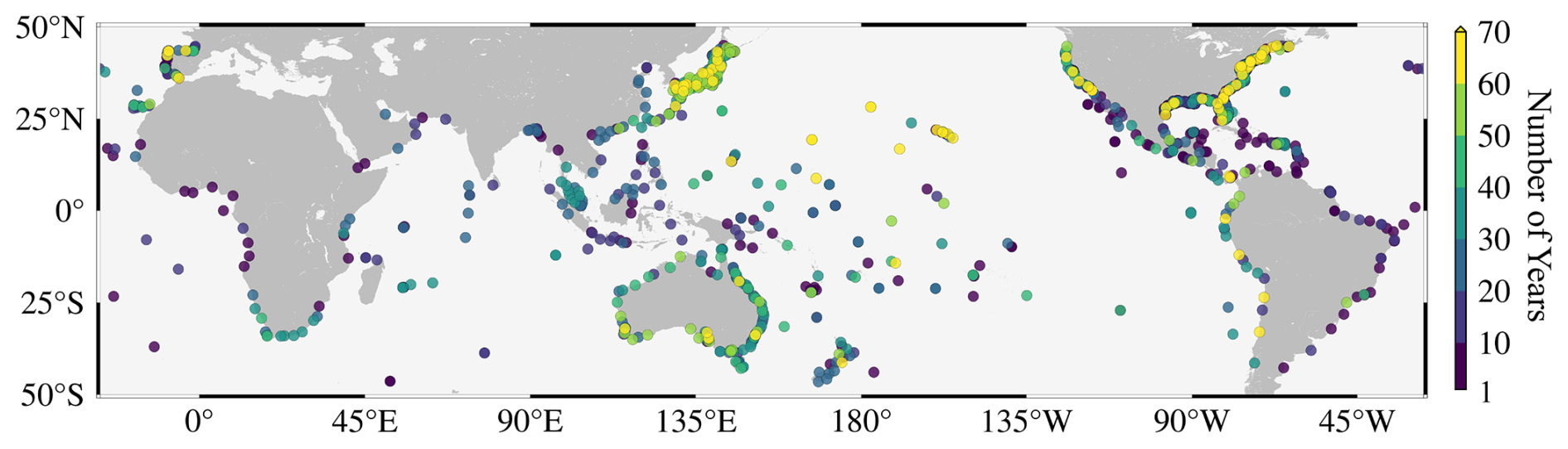
Figure 1 The distribution and data length of selected tide gauges.

2.3 Surge data simulated from a numerical model

Numerical model SSs came from GTSM version 3 global simulation forced with mean sea level pressure and wind from ERA5 (1979–2018), whose SS precision has been evaluated extensively and shown to have fair to good agreement with TG observations (Bloemendaal et al., 2019; Muis et al., 2020; Parker et al., 2023; Yang et al., 2023). This model was solved based on the Delft3D Flexible Mesh Suite (Kernkamp et al., 2011), with the unstructured grid resolution from 2.5 km (1.25 km in Europe) along the coast to 25 km in the deep ocean (Muis et al., 2020). It provided outputs both in the ocean and along the coastline; the latter's resolution was resampled to approximately every 20 km per coastal point to limit the data volume (Muis et al., 2020). Note that GTSM SSs were only used to assess our ASM data-driven model; they were not used in the training process of the latter.

2.4 Coastline contour data

The Global Self-consistent, Hierarchical, High-resolution Geography (GSHHG version 2.3.7) shoreline database (Wessel and Smith, 1996) was used to generate coastal nodes for ASM-SS in the research area (45° S–45° N). The shoreline of this dataset was developed from the World Vector Shorelines and Atlas of the Cryosphere, providing five different-resolution coastline contours (crude, low, intermediate, high, and full). We used the high-resolution data (∼300 m). After smoothing the shoreline with a window of 50 points, coastal nodes with a 10 km resolution were sampled evenly from the smoothed coastline. Figure 2 shows their distribution. The total number of nodes is 20 440: western Europe (200), Africa (2806), North America (3165), South America (2218), Oceania (3471), and Asia (8580).

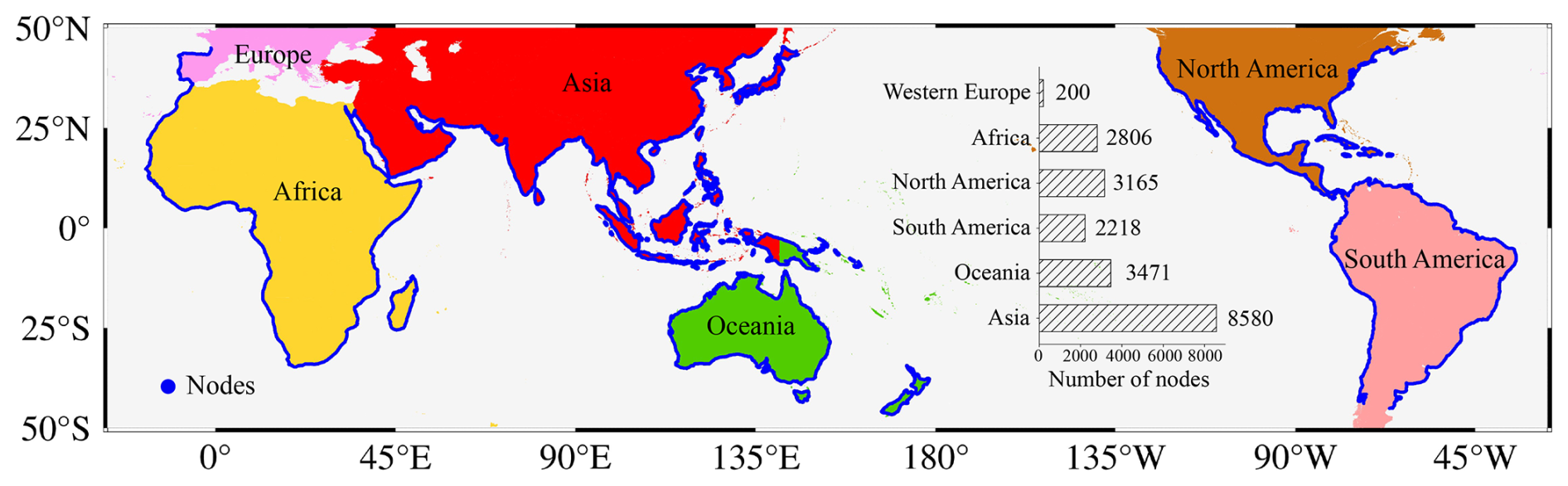
Figure 2 The distribution of coastal nodes for reconstructed storm surges.

2.5 All-site modeling framework

Full details of the ASM can be found in Yang et al.(2023). Here, a brief description of its modeling processes is provided, assuming that there are six available TGs within 45° S–45° N (Fig. 3a):

1. Obtaining predictors (Fig. 3b). Four atmospheric data (mslp, u10, v10, and t2m) for each TG station are extracted from the ERA5 dataset through linear interpolation. Changes in sea level pressure and wind are the main factors in generating SSs (Woodworth et al., 2019). Adding temperature variations considers the effects of thermal expansion and contraction. Meanwhile, following Yang et al. (2023, 2024b), another three variables (longitude, latitude, and time stamp) are considered since the geographical locations and record lengths of TGs are different. Hence, the predictor matrix for each TG consists of seven columns: mslp, u10, v10, t2m, longitude, latitude, and time.

2. All-site modeling (Fig. 3c). Predictor matrices and SSs of all six TG stations are stacked into one predictor matrix and one SS matrix. Then, the eXtreme Gradient Boosting Tree (XGBoost) (Chen and Guestrin, 2016) is used to learn the relationship between these two matrices. XGBoost is a residual machine learning model that generates a new decision tree using SS residuals from the previous tree. Therefore, the new tree will pay more attention to training where the residual errors are significant, making it suitable for modeling SS extremes.

3. Reconstruction (Fig. 3d). SSs can be estimated for any target node along the coastline by inputting the corresponding predictor matrix of that location into the model established in step 2.

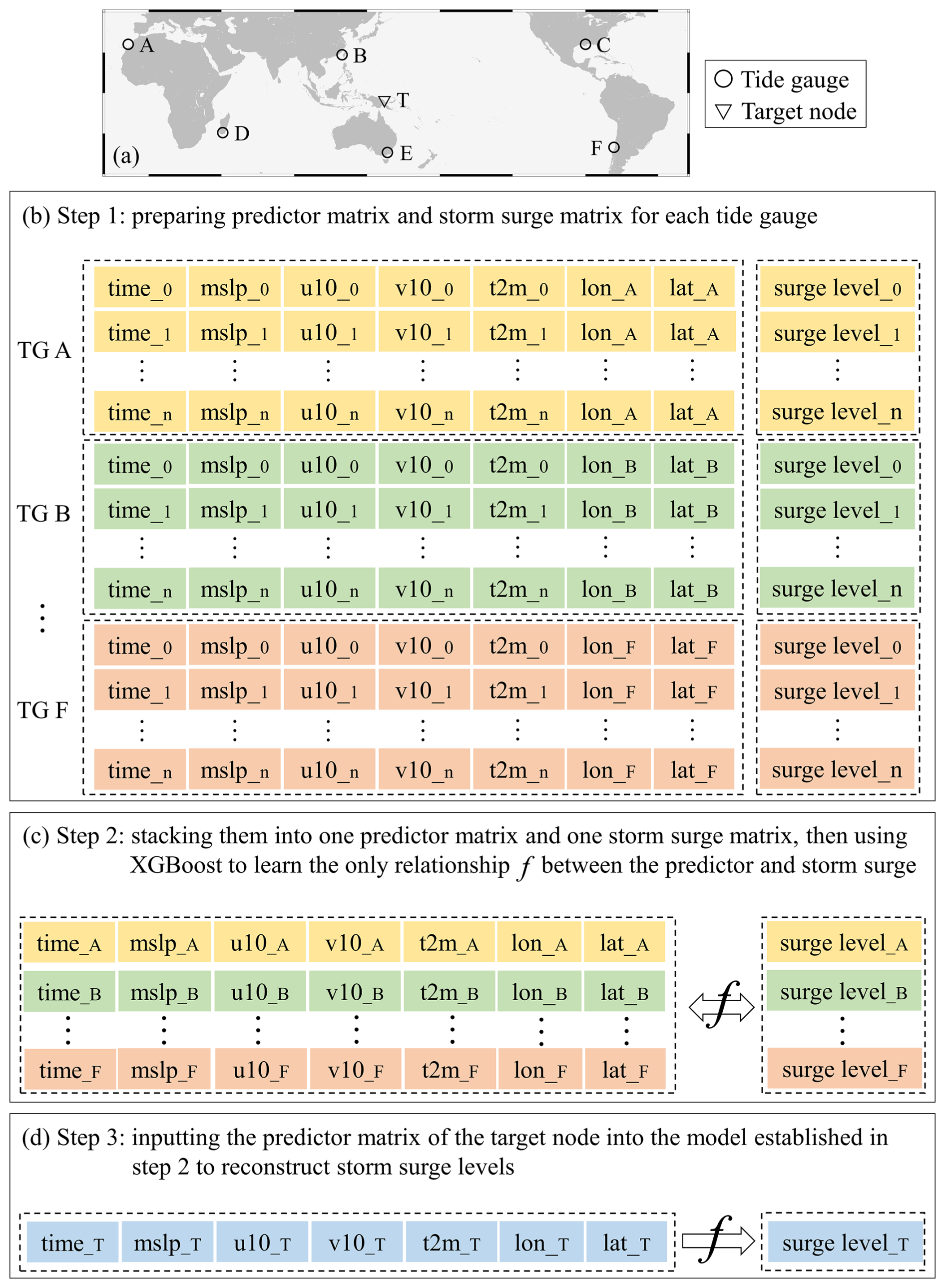
Figure 3 The modeling processes of the ASM framework.

2.6 Model performance metrics

Three model performance metrics are used to evaluate the differences between reconstructed and observed SS levels: Pearson product-moment correlation coefficient (CORR), root mean square error (RMSE), and mean bias (MB):

$$\begin{array}{}\text{(1)}& {\displaystyle }& {\displaystyle }\begin{array}{rl}{\displaystyle }& {\displaystyle }\text{CORR}=\\ {\displaystyle }& {\displaystyle \frac{{\sum }_{i=\mathrm{1}}^N({\text{SSL}}_{\mathrm{r},i}-\stackrel{\mathrm{‾}}{{\text{SSL}}_{\mathrm{r}}})({\text{SSL}}_{\mathrm{o},i}-\stackrel{\mathrm{‾}}{{\text{SSL}}_{\mathrm{o}}})}{\sqrt{{\sum }_{i=\mathrm{1}}^N({\text{SSL}}_{\mathrm{r},i}-\stackrel{\mathrm{‾}}{{\text{SSL}}_{\mathrm{r}}}{)}^{\mathrm{2}}}\sqrt{{\sum }_{i=\mathrm{1}}^N({\text{SSL}}_{\mathrm{o},i}-\stackrel{\mathrm{‾}}{{\text{SSL}}_{\mathrm{o}}}{)}^{\mathrm{2}}}}},\end{array}\text{(2)}& {\displaystyle }& {\displaystyle }{\displaystyle }{\displaystyle }\text{RMSE}=\sqrt{{\displaystyle \frac{{\sum }_{i=\mathrm{1}}^N({\text{SSL}}_{\mathrm{r},i}-{\text{SSL}}_{\mathrm{o},i}{)}^{\mathrm{2}}}{N}}},\text{(3)}& {\displaystyle }& {\displaystyle }{\displaystyle }{\displaystyle }\text{MB}={\displaystyle \frac{\mathrm{1}}{N}}{\sum }_{i=\mathrm{1}}^N({\text{SSL}}_{\mathrm{r}}-{\text{SSL}}_{\mathrm{o}}),\end{array}$$

where N is the length of the evaluation time series. SSL_r,i and SSL_o,i indicate the reconstructed and observed SS levels, respectively. $\stackrel{\mathrm{‾}}{{\text{SSL}}_{\mathrm{r}}}$ and $\stackrel{\mathrm{‾}}{{\text{SSL}}_{\mathrm{o}}}$ are their average values.

3 Results

3.1 ASM evaluation at tide gauges

The k-fold cross-validation strategy was chosen to evaluate the ASM at TGs; 823 TG stations with time lengths exceeding 10 years between 1940 and 2020 were randomly divided into 10 parts (i.e., 10-fold cross-validation), with the last part containing 85 TGs. Each time, nine of the parts were used for training. After the model was established, predictor matrices of the excluded TGs were inputted into the model to obtain their SSs. The SSs of all of the TGs can be estimated once each part has been excluded. Then, we compared the reconstructed entire surge time series (evaluating the overall variation trend) and the 95th percentile SSs (assessing extreme events) with TG observations. As shown in Fig. 4 and Table 1, we divided the research area into 15 subregions (ER: the equatorial region, WEU: western Europe, NAF: northern Africa, SWA: southwestern Africa, SEA: southeastern Africa, WNA: western North America, ENA: eastern North America, CA: Central America, SWS: southwestern South America, SES: southeastern South America, WAS: western Asia, EAS: eastern Asia, SAS: southern Asia, NOC: northern Oceania, and SOC: southern Oceania) for more detailed assessment information. Note that the equatorial region (∼6° S–∼6° N) was separated as an independent area since it has almost no tropical cyclones.

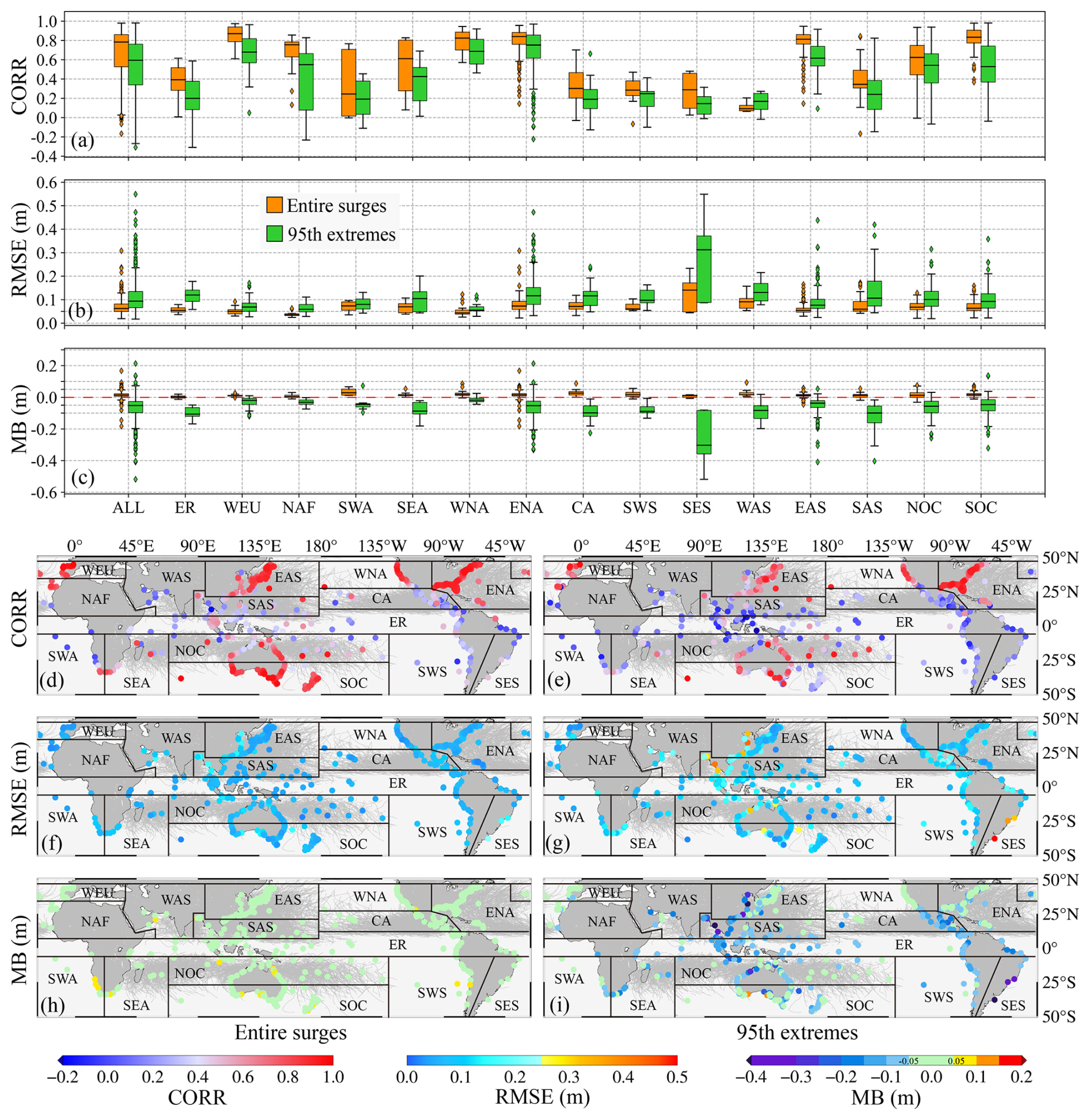
Figure 4 ASM evaluation at tide gauges from 1940 to 2020. (a–c) Entire surge and 95th extreme evaluation statistics for the different regions. (d–i) Distributions of the evaluation metrics. The gray lines are tropical cyclone paths from Gahtan et al. (2024).

Table 1 The medians of the evaluation statistics for the different regions in Fig. 4.

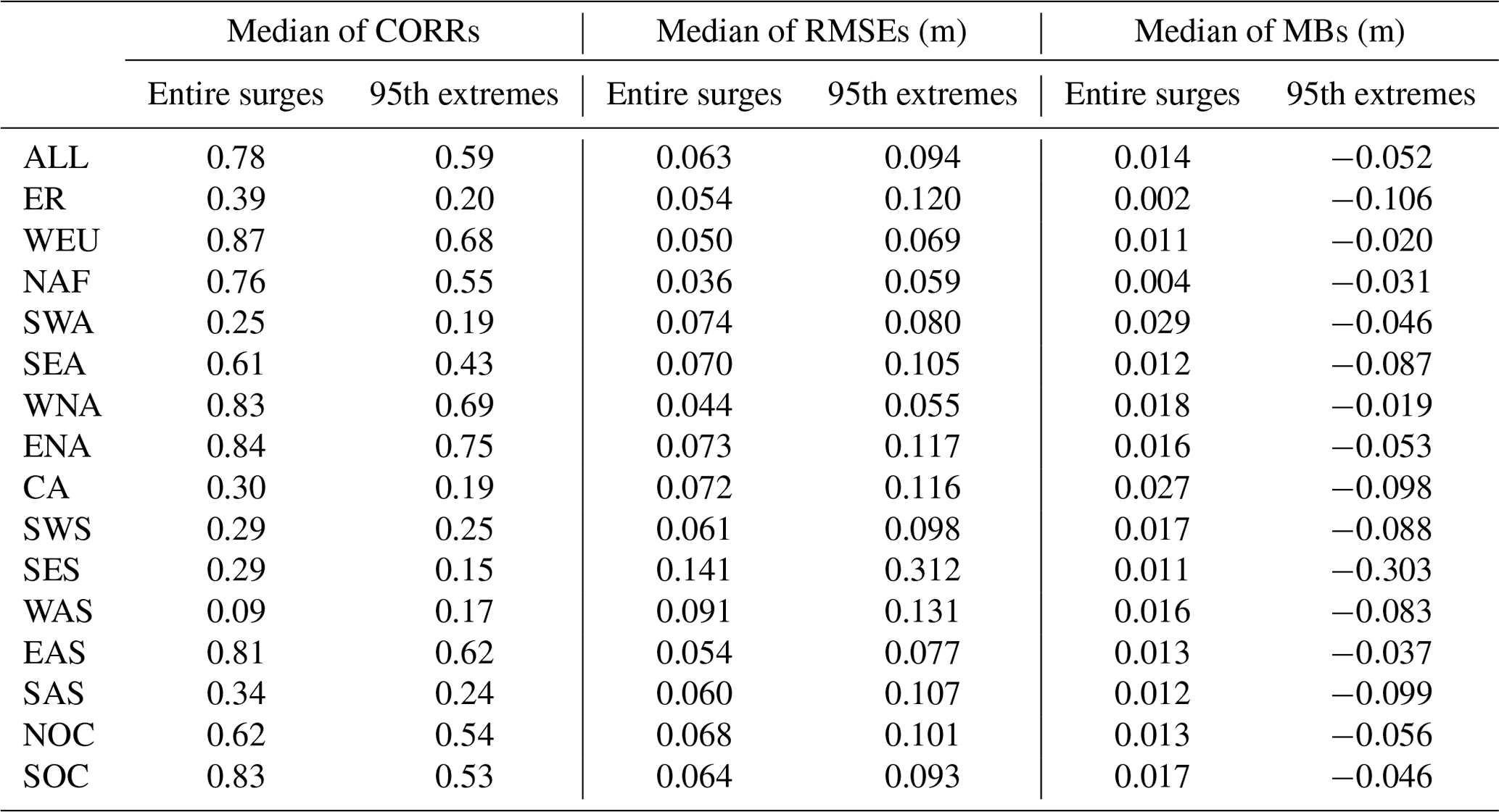
Figure 4a–c and Table 1 show that, on a quasi-global scale (i.e., for ALL TGs), the median CORR of the entire time series of surges is 0.78, the RMSE is 0.063 m, and the MB is 0.014 m. In comparison, the reconstruction precision for extreme events (>95th percentile) is lower: the CORR is 0.59, the RMSE is 0.094 m, and the MB is −0.052 m (indicating a slight underestimation of the magnitudes of extreme events). At the regional scale, there are differences between subregions (Fig. 4d–i). In areas with almost no tropical cyclones, including ER, SWA, SWS, and SES, the precision is low for both entire surges and 95th extremes. For other places, the precision of estimated SSs is better in regions with a relatively high density of TG stations, such as WEU, WNA, ENA, EAS, NOC, and SOC. This result is consistent with the conclusion of Yang et al. (2024b) that reducing the spatial interval of TG stations can benefit the estimation of SSs, especially the extremes.

It is necessary to evaluate temporal variations in reconstructed SSs further since their length is over 80 years, during which time the number of TG stations and the quality of the atmospheric data change. As shown in Fig. 5, the precision of ASM at the TGs in each subregion was calculated every 10 years (excluding TGs with less than 1 year of data in a given decade). Results indicate that the overall precision (i.e., for ALL TGs) of entire surges and 95th extremes gradually increased from 1940 to 2020. Possible reasons are as follows: on the one hand, ASM is affected by the spatial resolution of TGs (Yang et al., 2024b). The increase in TGs in recent decades (Haigh et al., 2023) has enhanced its precision. On the other hand, the quality of the ERA5 data has improved as more satellite data have been assimilated since the 1970s (Soci et al., 2024), which benefits the data-driven model. At the regional scale, for entire surges, Fig. 5a indicates that, except for SWA (CORR decreases) and WAS (CORR remains unchanged), the CORRs of the other subregions present an upward trend: Fig. 5b shows the RMSE in SES increases, while the RMSEs in the other regions decrease. Figure 5c shows that the MBs of the subregions have gradually been optimized (excluding WAS). For 95th extremes, in terms of CORRs (Fig. 5d), WEU, NAF, WNA, ENA, EAS, NOC, and SOC show an upward trend, whereas there is no obvious pattern in the other regions. For RMSEs (Fig. 5e), ER, SEA, and SES present an increasing trend, while the other regions decrease. For MBs (Fig. 5f), the underestimation of SSs in ER and SAS rises, and there is no noticeable change in WNA and SES. MBs in WEU, NAF, ENA, WAS, EAS, NOC, and SOC are optimized, while there is no clear pattern in SWA, SEA, CA, and SWS.

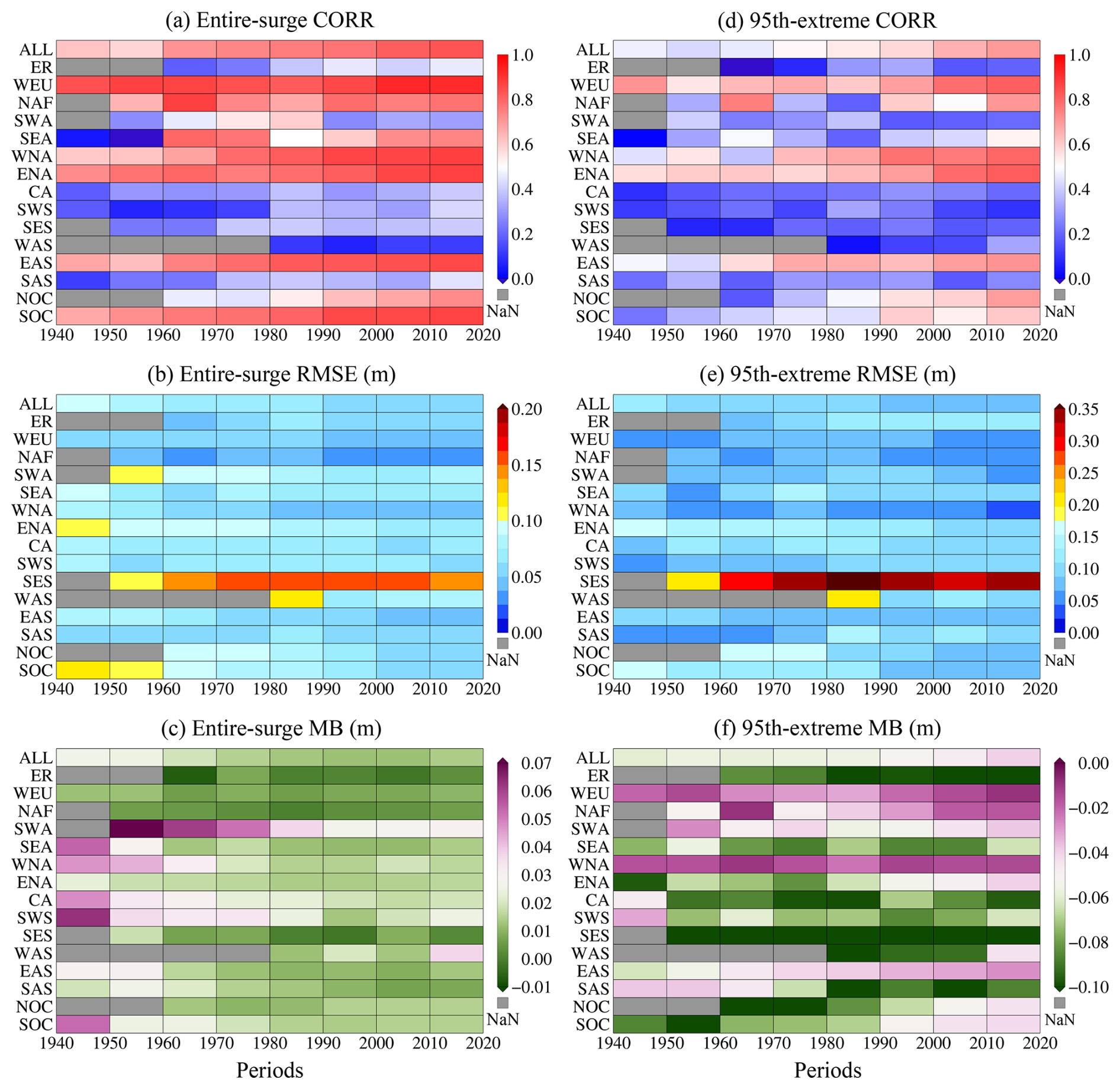
Figure 5 Temporal variations of the ASM precision at tide gauges from 1940 to 2020. (a–c) Entire surge evaluation statistics for the different regions every 10 years. (d–f) The 95th extreme evaluation statistics for the different regions every 10 years.

3.2 ASM comparison with a numerical model at the tide gauge scale

Since GTSM provided numerical surges from 1979 to 2018, ASM data in the same period were extracted from SSs reconstructed in Sect. 3.1. In addition, since points of GTSM did not completely coincide with TG stations, linear interpolation was used to interpolate GTSM SSs to the corresponding TG locations. Figure 6 and Table 2 give the 95th extreme comparison results between ASM, GTSM, and TG observations.

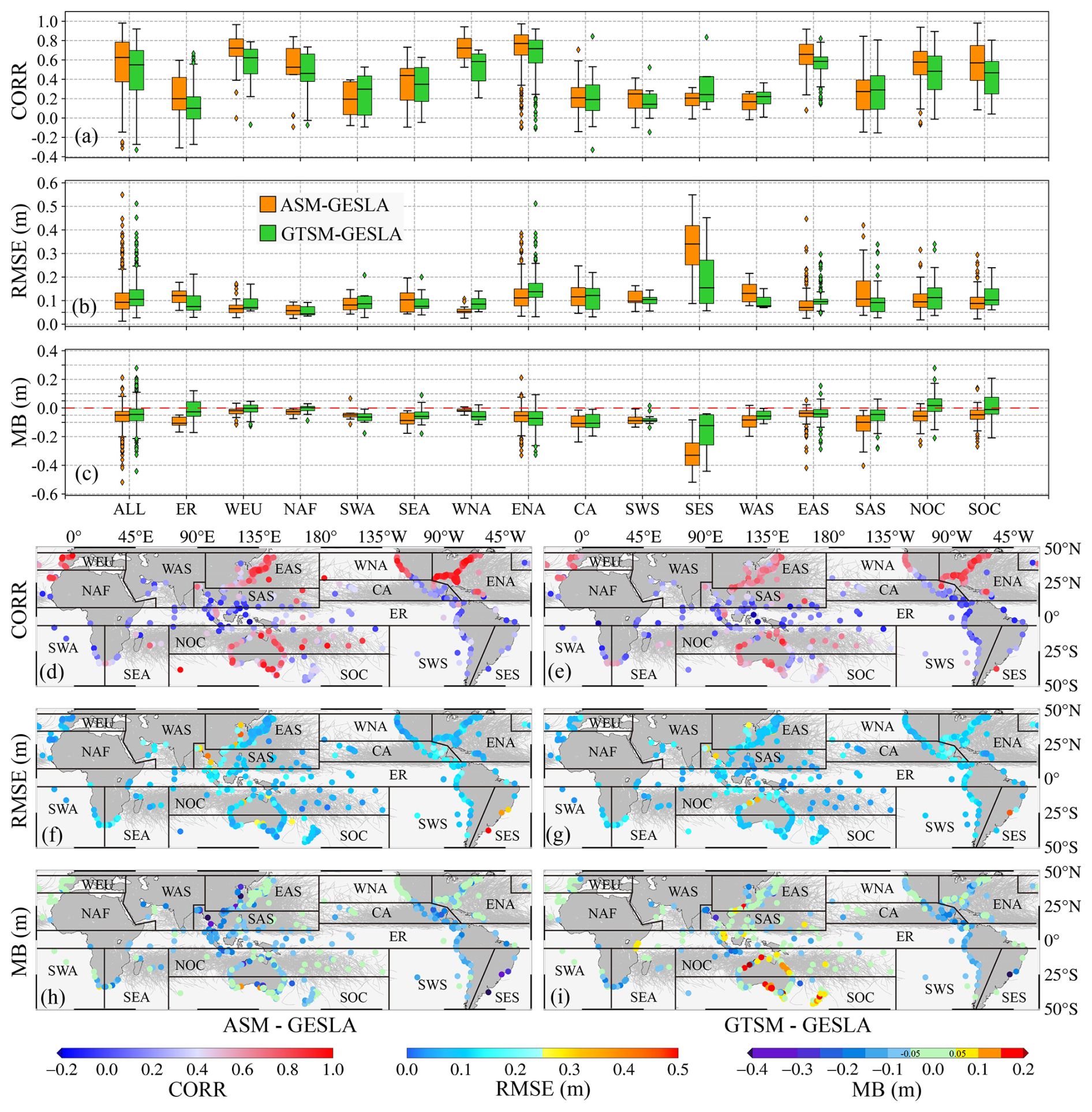
Figure 6 ASM comparison with the numerical model at tide gauges from 1979 to 2018. (a–c) ASM and GTSM 95th extreme evaluation statistics for the different regions. (d–i) Distributions of the evaluation metrics. The gray lines are tropical cyclone paths from Gahtan et al. (2024).

Table 2 The medians of the evaluation statistics for the different regions in Fig. 6.

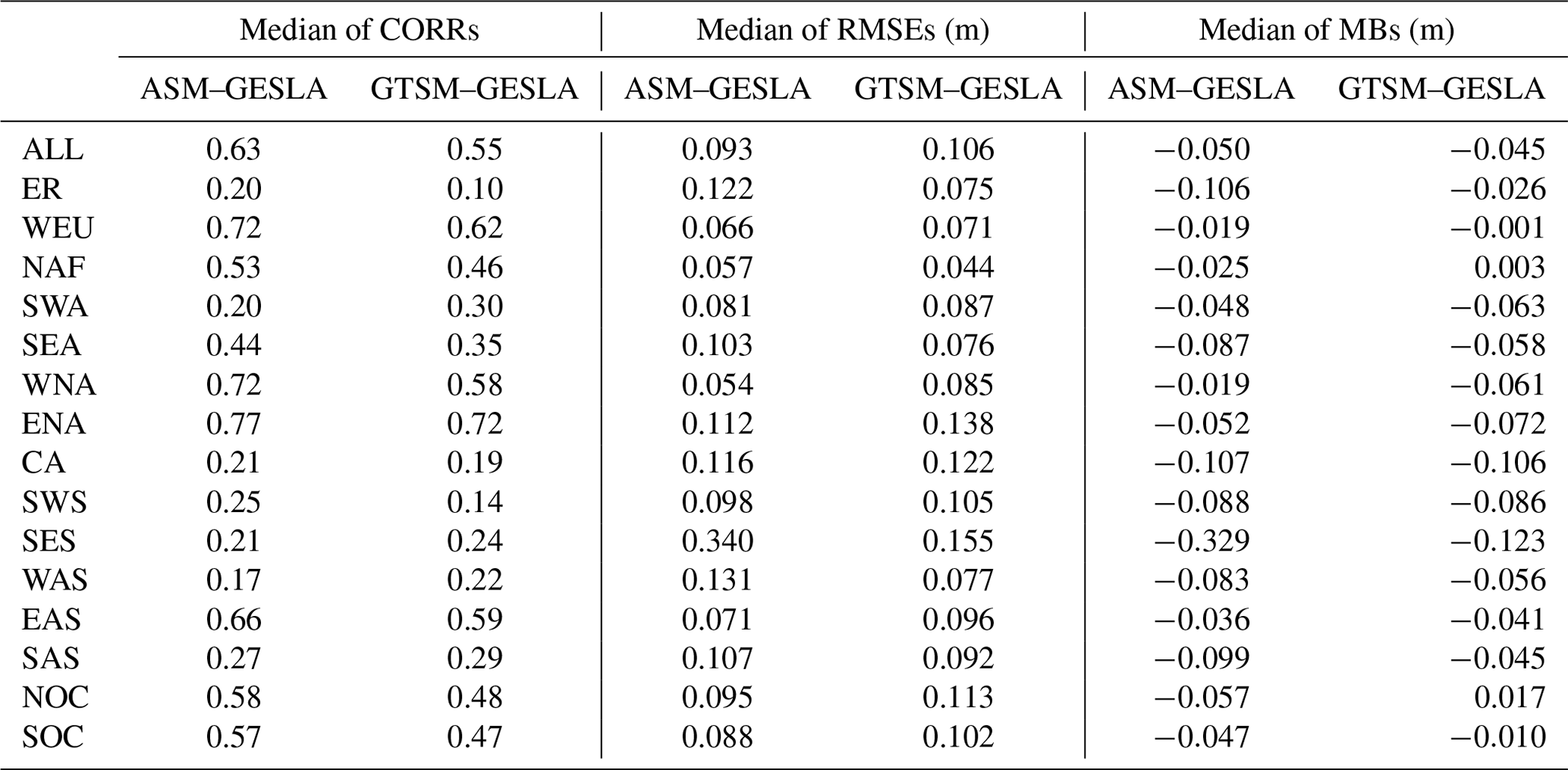
It can be seen from Fig. 6a–c and Table 2 that, on the quasi-global scale, ASM (the medians of CORRs, RMSEs, and MBs for the 95th extremes are 0.63, 0.093, and −0.050 m, respectively) outperforms the numerical GTSM (the medians are 0.55, 0.106, and −0.045 m). At the regional scale (Fig. 6d–i), ASM and GTSM perform poorly in areas with no tropical cyclones (ER, SWA, SWS, and SES), indicating that, in addition to meteorological factors, oceanographic processes in these regions contribute to the extremes (Cid et al., 2017; Woodworth et al., 2019). For areas severely affected by tropical cyclones (such as WEU, WNA, ENA, EAS, NOC, and SOC), ASM and GTSM are more precise. Moreover, the CORRs and RMSEs of ASM are better than those of GTSM in these subregions, while the MBs of GTSM are closer to 0 m in WEU, NOC, and SOC (Fig. 6a–c). However, GTSM appears to overestimate extremes in some areas, such as NOC and SOC (Fig. 6i). For further insight, Fig. 7 presents scatter density plots of ASM and GTSM annual maximum SSs compared with TG records. Of the 15 subregions, the determination coefficient (R²) of ASM in 10 of them is better than that of GTSM (Fig. 7b–i, k, and o); the RMSE of ASM is smaller than that of GTSM in 12 areas (Fig. 7b–j, m, o, and p). However, there are two subregions where the R² and RMSE of ASM are worse than those of GTSM (Fig. 7l and n), possibly because the available TGs are sparse, especially in WAS. On a quasi-global scale, ASM's overall RMSE and R² improvements compared to GTSM are 22.3 % (from 0.184 to 0.143 m) and 14.8 % (from 0.61 to 0.70), respectively (Fig. 7a), which means that ASM is more stable than GTSM. The reason why ASM outperforms GTSM could be two main aspects. For the global numerical GTSM, as mentioned in the Introduction section, the accuracy and spatial resolution of bathymetric data in the nearshore area limit the precision of SSs. Meanwhile, the grid with a resolution of several kilometers affects the effective simulation of small-scale physical factors. For the ASM data-driven model, the training process is based on TG observations. TGs are the most accurate source for sea level monitoring, and their records can be considered to include effects from all spatial-scale physical processes. In addition, the machine learning method XGBoost is a residual model that pays more attention to where residual errors are significant, which also benefits the estimation of extreme SSs.

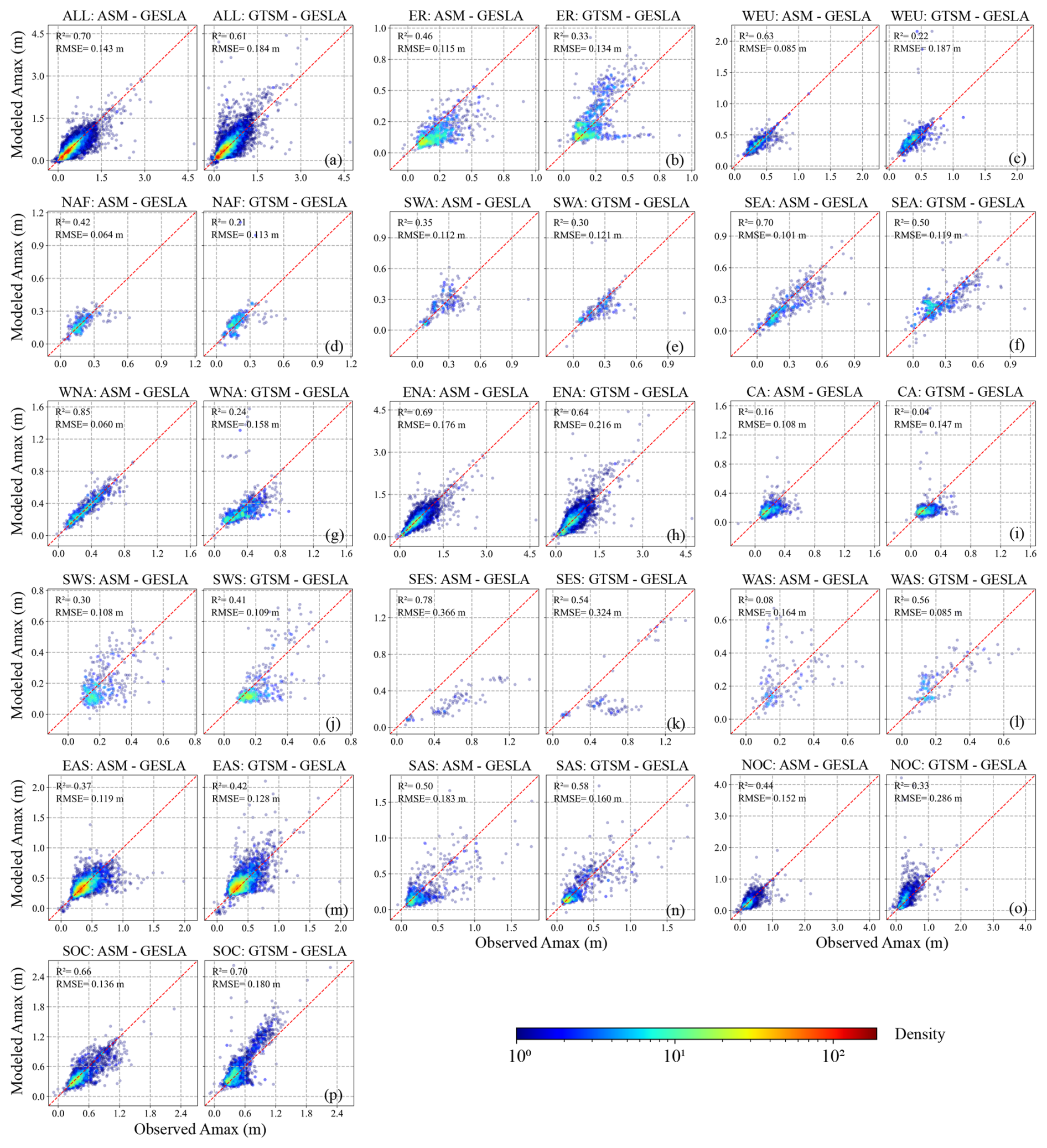
Figure 7 Scatter density plots of ASM and GTSM annual maxima (Amax) compared with tide gauge observations in the different regions. The data for the tide gauges were combined. The red dotted line indicates the perfect-fit line.

3.3 ASM comparison with a numerical model at the coastal scale

As mentioned in the Introduction section, though ASM and single-site modeling belong to the data-driven model, the former can provide SS information for ungauged points since their basic ideas differ. This advantage of ASM allows us to compare the data-driven model and numerical model on a quasi-global scale with high spatial resolution. In this section, the ASM was trained based on all 1315 TGs within the research area with records longer than 1 year from 1940 to 2020 (Fig. 1). Then SSs from 1979 to 2018 were reconstructed to all coastal points of GTSM to assess their differences (Fig. 8 and Table 3).

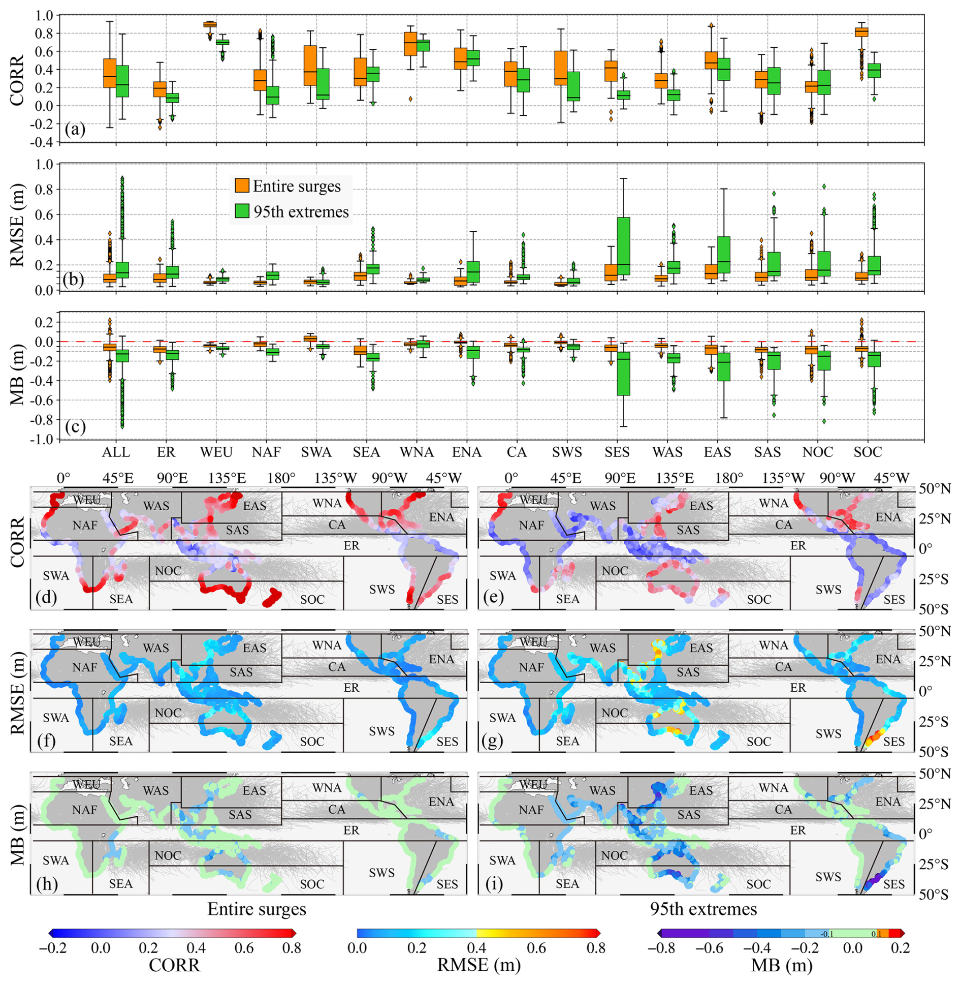
Figure 8 Differences between ASM and GTSM at the coastal scale from 1979 to 2018. (a–c) Comparison model statistics between ASM and GTSM entire surges and 95th extremes for the different regions. (d–i) Distributions of the comparison metrics. The gray lines are tropical cyclone paths from Gahtan et al. (2024).

Table 3 The medians of the evaluation statistics for the different regions in Fig. 8.

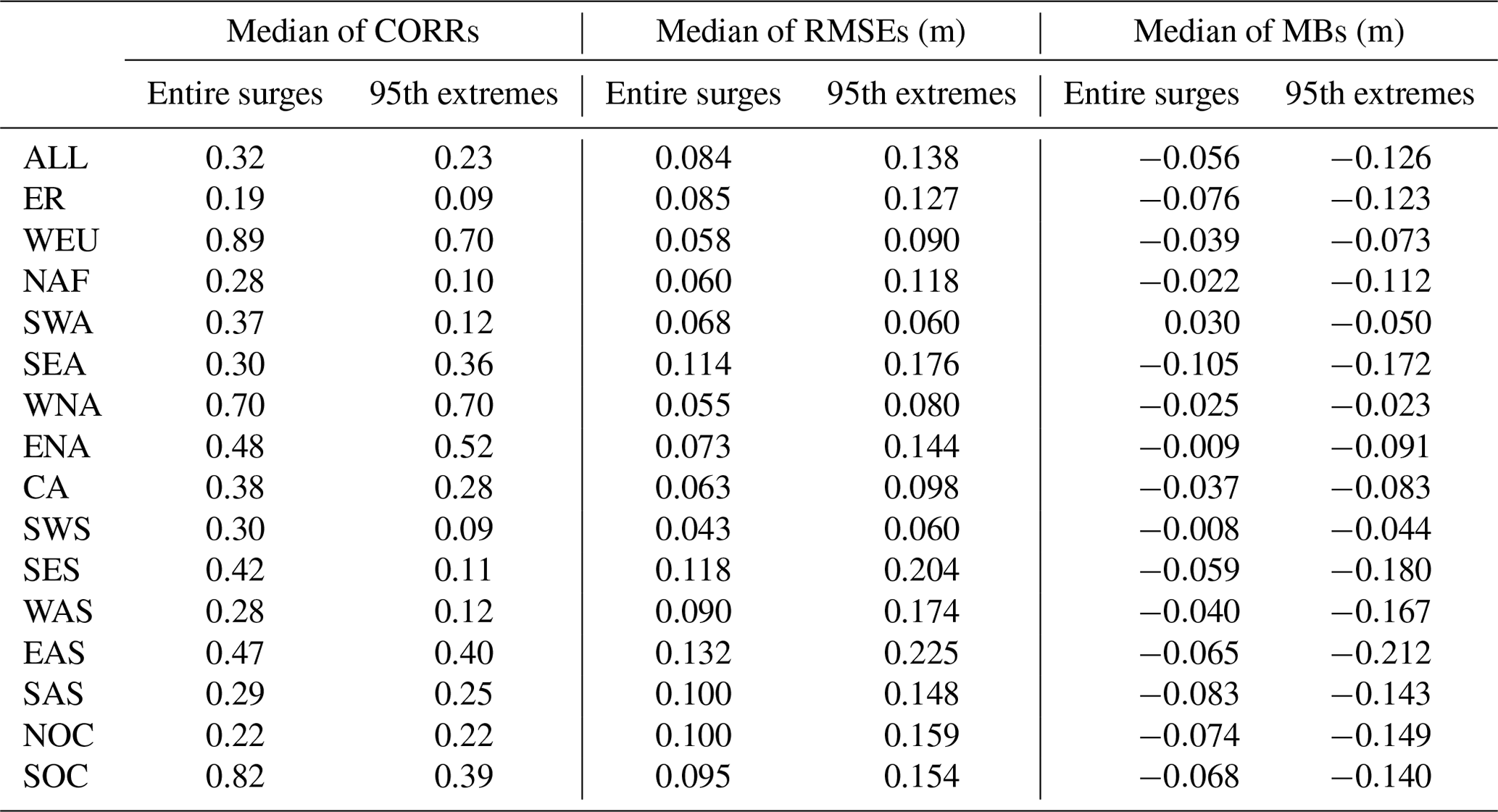
Figure 8 and Table 3 give the comparison results between ASM and GTSM entire surges and 95th extremes. Note that, since both ASM and GTSM SSs were estimated, we used GTSM as the baseline here. As shown in Fig. 8 and Table 3, there are noticeable differences between ASM and GTSM. On the quasi-global scale, the medians of the CORRs, RMSEs, and MBs of the entire surges (95th extremes) between them are 0.32 (0.23), 0.084 m (0.138 m), and −0.056 m (−0.126 m), respectively (Fig. 8a–c). The negative MBs indicate that ASM tends to give lower SS estimates than GTSM, which is consistent with the conclusion from the comparison with TGs in Sect. 3.2. From a regional perspective, the agreement between ASM and GTSM (Fig. 8d, f, and h for entire surges and Fig. 8e, g, and i for 95th extremes) is better in WEU, SEA, WNA, ENA, EAS, and SOC. For the other places, on the one hand, both ASM and GTSM showed relatively poor agreement with TG observations in Sect. 3.2 (Fig. 6d–i); on the other hand, there are also visible discrepancies between ASM and GTSM (Fig. 8d–i). Possible reasons could be as follows: for ASM, its extreme SS reconstruction is affected by the distribution and spatial intervals of TG stations (Yang et al., 2024b). For GTSM, the grid resolution and the bathymetric data's precision also impact the simulation results. Additionally, neither of them considers sea level variations caused by runoff and precipitation. Nevertheless, the precision of ASM and GTSM for these regions needs further improvement in the future.

4 Data availability

The ASM-SS quasi-global storm surge dataset was generated from the ASM data-driven model established in Sect. 3.3. The dataset is available month by month at https://doi.org/10.5281/zenodo.14034726 (Yang et al., 2024a) as NetCDF files from 1940 to 2020. Each file includes five parameters: longitude, latitude, nodes, time, and surge level. Longitude and latitude are the location information of nodes in degrees. The time unit is accumulated hours since 1900-01-01 00:00:00. The surge levels are given in meters. Users can use longitude, latitude, and time as keywords to select surge levels at nodes of interest within a target period. In addition, the spatial resolution of the nodes is 10 km along the coastline (as shown in Fig. 2). Since the sea surface varies rapidly during tropical cyclones, the temporal resolution of surge levels is set to hourly. Though this temporal resolution increases the data volume, it can provide sufficient information for users who want to analyze high-frequency variations of storm surges during extreme events.

5 Conclusion and discussion

High-spatial-coverage and long-term SS records are the basis for deepening our understanding and better preparing coastal communities for incoming ESLs. However, high-spatial-resolution SS information on a global or quasi-global scale can only be simulated by global numerical models due to the sparse and uneven distribution of TG stations. Here, based on the ASM framework, we established a SS data-driven model using observations from TGs between 45° S and 45° N. Then, for the first time, a high-spatial-resolution (every 10 km per node along the coastline), long-term (over 80 years from 1940 to 2020), quasi-global (within 45° S–45° N), and hourly data-driven SS dataset (ASM-SS) was reconstructed from this ASM. Evaluation results indicate that, for 95th extreme SSs, this model (the medians of the CORRs, RMSEs, and MBs are 0.63, 0.093, and −0.050 m, respectively) is better than the state-of-the-art hydrodynamic GTSM (the medians are 0.55, 0.106, and −0.045 m); for annual maximum SSs, ASM is more stable than GTSM, with the overall RMSE and coefficient of determination optimizing by 22.3 % and 14.8 %, respectively. This dataset could provide possible alternative support aside from numerical models for coastal communities to analyze variations of SSs, the contribution of SSs to ESLs, and other relevant applications.

Nonetheless, several details of this model can be studied more deeply in our future work: (1) generally speaking, tropical cyclones are accompanied by heavy rainfall when they make landfall, which might affect sea surface height. In addition, the impact of river runoff in estuarine areas may need to be considered. (2) The distribution and spatial intervals of TG stations have been proven to affect the precision of ASM (Yang et al., 2024b). Because establishing and maintaining a permanent TG network with high spatial coverage in coastal regions is expensive and complex, it is necessary to consider integrating various water level observation technologies, such as Global Navigation Satellite System reflectometry (GNSS-R) and satellite altimetry. (3) From the predictor side, several studies showed that ERA5 data tend to relatively underestimate higher wind speeds (Graham et al., 2019; Xiong et al., 2022), which may lead to underestimations of extreme SSs. Therefore, the atmospheric predictors can also be optimized through multisource data fusion, such as considering wind speeds obtained from spaceborne GNSS-R (e.g., the Cyclone Global Navigation Satellite System) or cyclone information obtained from remote sensing satellites.