Machine-learning-based reconstruction of long-term global terrestrial water storage anomalies from observed, satellite and land-surface model data

Understanding long-term terrestrial water storage (TWS) variations is vital for investigating hydrological extreme events, managing water resources and assessing climate change impacts. However, the limited data duration from the Gravity Recovery and Climate Experiment (GRACE) and its follow-on mission (GRACE-FO) poses challenges for comprehensive long-term analysis. In this study, we reconstruct TWS anomalies (TWSAs) for the period from January 1960 to December 2022, thereby filling data gaps between the GRACE and GRACE-FO missions and generating a complete dataset for the pre-GRACE era. The workflow involves identifying optimal predictors from land surface model (LSM) outputs, meteorological variables and climatic indices using a novel Bayesian network (BN) technique for raster-based TWSA simulations. Climate indices, like the Oceanic Niño Index and Dipole Mode Index, are selected as optimal predictors for a large number of grid cells globally, along with TWSAs from LSM outputs. The most effective machine learning (ML) algorithms among convolutional neural network (CNN), support vector regression (SVR), extra trees regressor (ETR) and stacking ensemble regression (SER) models are evaluated at each grid cell to achieve optimal reproducibility. Globally, ETR performs best for most of the grid cells; this is also noticed at the river basin scale, particularly for the Ganga–Brahmaputra–Meghna, Godavari, Krishna, Limpopo and Nile river basins. The simulated TWSAs (BNML_TWSA) outperformed the TWSAs from LSM outputs when evaluated against GRACE datasets. Improvements are particularly noted in river basins such as the Godavari, Krishna, Danube and Amazon, with median correlation coefficient, Nash–Sutcliffe efficiency, and RMSE values for all grid cells in the Godavari Basin, India, being 0.927, 0.839 and 63.7 mm, respectively. A comparison with TWSAs reconstructed in recent studies indicates that the proposed BNML_TWSA outperforms them globally as well as for all of the 11 major river basins examined. Furthermore, the uncertainty of BNML_TWSA is assessed for each grid cell in terms of the standard error. Results show smaller standard error magnitudes in grid cells in arid regions compared to other regions. The presented gridded dataset is published at https://doi.org/10.6084/m9.figshare.25376695 (Mandal et al., 2024), featuring a spatial resolution of 0.50° × 0.50° and offering global coverage.

1 Introduction

Terrestrial water storage (TWS) refers to the storage of water on or above the surface of the Earth, including hydrological elements such as groundwater, soil moisture, snow, ice and surface water (Yu et al., 2021; Yang et al., 2021). The fluctuations in TWS in both space and time have been comprehensively simulated by employing physically based land surface models (LSMs) and global hydrological models (GHMs) (Humphrey et al., 2017; Felfelani et al., 2017; Sun et al., 2021). These models have significant biases due to inherent uncertainty and the inadequate representation of some physical processes, such as the lack of modeling of human water resource interventions within LSMs (Bibi et al., 2024). Furthermore, in snow-dominated basins, LSMs often underestimate peak terrestrial water storage anomalies (TWSAs), whereas GHMs tend to overestimate them. Similarly, in temperate, arid and tropical basins, both model types generally underestimate TWSA peaks (Bibi et al., 2024), which limits the application of these model outputs for long-term analyses of climate change impact assessment, water resource management and hydrological extreme event forecasting. The Gravity Recovery and Climate Experiment (GRACE) mission and its successor GRACE Follow-on (GRACE-FO) have been providing unprecedented accurate measurements of TWSAs since April 2002 (Mo et al., 2022). These TWSA observations have been widely used in hydrological studies to assess the impacts of climate change and human activities on large-scale water balance, droughts and floods, and groundwater storage (Rodell et al., 2018). Similar to other satellite observations, the GRACE mission has data gaps, such as an 11-month gap between the end of the GRACE mission in June 2017 and the start of the GRACE-FO mission in May 2018 as well as an additional few months of data gap during each mission.

A reliable, long-term, continuous TWSA dataset is imperative for the assessment of basin-scale water balance and local hydrological extremes. Different studies have employed various techniques to reconstruct long-term TWSAs beyond the GRACE period. In a study by Becker et al. (2011), the authors integrated spatial patterns of TWS derived from GRACE data with long-term in situ river level records to recreate the TWS for the Amazon Basin from 1980 to 2008. Forootan et al. (2014) developed an autoregressive model with exogenous variables (ARX), a statistical data-driven approach, to reconstruct TWSAs for West Africa using the GRACE dataset; rainfall data from the Tropical Rainfall Measuring Mission (TRMM); and sea surface temperature (SST) information spanning the Atlantic, Indian and Pacific oceans. Ahmed et al. (2019) employed an ARX model to establish a relationship between GRACE TWS and meteorological variables, as well as vegetation indices. Nie et al. (2016) utilized the Global Land Data Assimilation System (GLDAS) products and GRACE-based TWSA data to reconstruct TWSAs using the water balance approach from 1948 to 2012 over the Amazon Basin. Humphrey et al. (2017) established a statistical data-driven model that linked GRACE TWSAs with deviations in both temperature and precipitation to recreate TWSAs from 1985 to 2015 for the entire globe.

Machine-learning-based algorithms have gained popularity over the past 2 decades, presenting new opportunities in hydrology and related fields, including the reconstruction of TWSAs. Long et al. (2014) made one of the first attempts to hindcast TWSAs for the period from February 1979 to September 2012 by developing an artificial neural network (ANN) model using GRACE data and other in situ modeling data to study extreme climate events in the Yungui Plateau, China. Sun et al. (2019) used a deep convolutional neural network (CNN) with three model architectures to predict the spatiotemporal variations in TWSAs over India. Similarly, Li et al. (2020) and Sun et al. (2020) utilized multiple linear regression (MLR) and neural-network-based models, in conjunction with ARX, to reconstruct TWSAs globally. Jing et al. (2020) generated a GRACE-like TWSA prior to the GRACE period, dating back to 1979, over the Nile Basin using the Random Forest and eXtreme Gradient Boosting ensemble learning algorithms. Yu et al. (2021) used three deep learning models to hindcast TWSAs over Canada from 1972 to 2002 based on land surface model (LSM) output as a predictor. Satish Kumar et al. (2023) reconstructed GRACE-like time series of TWSAs from 1960 to 2016 across four river basins in southern India.

The reconstruction of TWSAs has been a significant area of research, with studies such as that by Sun et al. (2020) emphasizing the need to enhance the performance accuracy of machine learning (ML) and statistical algorithms. Most global TWSA reconstruction studies primarily employ a single ML algorithm to model TWSAs (Sun et al., 2020; Mo et al., 2022; Li et al., 2020). However, some studies, including those by Li et al. (2020) and Sun et al. (2020), also employ statistical algorithms in conjunction with ML. Consequently, the reliance on a single ML algorithm for each grid cell presents a limitation that needs to be addressed to improve the robustness and accuracy of TWSA reconstructions. Different algorithms have varying strengths with respect to handling the nonlinearities and complexities inherent in regional hydrological systems. Testing multiple ML algorithms can ensure methodological robustness and help identify the appropriate approach for TWSA reconstruction.

The ML models used in hydrological studies so far can be broadly divided into two main categories: single-algorithm usage and multiple-algorithm usage. Most ML investigations predominantly belong to a single-algorithm-usage category, where the performance of a specific algorithm is evaluated against the baseline performance (Raghavendra and Deka, 2014; Sun et al., 2014; Mo et al., 2022; Khan and Maity, 2020). Other studies compare the performance of different ML models with the aim of finding the best algorithm, which performs well across a wide range of situations (Mandal and Chanda, 2023; Sun et al., 2021). Using a single-algorithm approach could prove satisfactory when dealing with a compact research area or multiple study areas with similar hydroclimatic characteristics. However, it becomes insignificant for large study areas, multi-site analysis with different hydroclimatic conditions and in cases where the relative importance of predictors can vary spatially. This may greatly affect the final performance of ML models. Previous studies on grid-cell-scale reconstruction of GRACE TWSAs indicate that there is no individual algorithm that consistently outperforms others across all global basins (Sun et al., 2020, 2021; Li et al., 2020). Sun et al. (2020) found that a deep neural network model performed better than the other two data-driven methods for reconstructing TWSAs over global river basins at a grid cell scale. Mo et al. (2022) employed Bayesian convolutional neural networks (BCNNs) to reliably interpolate the TWSA data gap between GRACE and GRACE-FO globally. Deep convolutional autoencoders outperform CNNs and BCNNs when filling the gaps between GRACE and GRACE-FO globally (Uz et al., 2022). The integrated CNN-based support vector machine has been found by Kalu et al. (2023) to outperform other regression models in the Congo Basin, Africa.

In recent times, a relatively new approach has been adopted by many studies, wherein the optimal features are selected before applying a single and/or multiple ML algorithms to evaluate the prediction accuracy (Das and Chanda, 2020; Das et al., 2022). The significance of predictor selection has been emphasized by several studies, which point out the inadequacies of current algorithms for identifying efficient or optimal predictors (Mo et al., 2022; Sun et al., 2020; Li et al., 2020). Sun et al. (2020) specifically raises concerns about determining which set of predictors or predictor groups play a more significant role, which is crucial for enhancing the interpretability and explainability of ML solutions. To the best of our knowledge, the selection of optimal predictors for the reconstruction of TWSAs using Bayesian networks is exercised for the first time in this study, which also highlights the novelty of the study. Selection of optimal predictors is not only a methodological novelty but also a critical step to ensure that the model prioritizes the most relevant and physically meaningful predictors. This approach reduces noise, minimizes overfitting and enhances interpretability, making the final product more scientifically robust and practically useful (Das and Chanda, 2024).

In the present study on the reconstruction of TWSAs, the potential of Bayesian networks is utilized for the selection of optimal predictors from a broad set of inputs comprising observed, satellite and land-surface-based data products. The input and target datasets are used without prior interpolation of intermittent gaps, detrending, deseasoning or decomposing signals, in order to prevent the introduction of bias. We applied different ML models to each global grid cell in this study and selected the most appropriate model for each grid cell based on their performance to ensure optimal reproducibility. Furthermore, we conduct the analysis at the basin scale across 11 global river basins with varied hydroclimatic characteristics from six different continents: Amazon, Danube, Ganga–Brahmaputra–Meghna (GBM), Godavari, Indus, Krishna, Limpopo, Mississippi, Murray–Darling, Nile and Zambezi. Among these rivers, the Amazon, GBM and Mississippi exhibit humid hydrologic characteristics, while the Nile is semiarid and the Zambezi is semi-humid (Uz et al., 2022). Furthermore, a diverse range of basin sizes has been taken into account, spanning from the vast Mississippi Basin, which covers 2 918 820 km², to the relatively small Krishna Basin, with an area of 258 948 km². The study aims to achieve three objectives. First, it aims to specifically select the optimal predictors for TWSAs from a number of meaningful inputs, including LSM outputs, meteorological variables and climate indices, for each grid cell, utilizing the potential of Bayesian networks. Second, it aims to select a leader model for each grid cell from a number of ML models, including kernel-based, network-based and ensemble models, based on their performance. Finally, it aims to simulate GRACE-like TWSAs and reconstruct a global TWSA datasets for the historical period starting from 1960 and including the data gap periods of the GRACE and GRACE-FO missions.

In the rest of the paper, Sect. 2 describes the data used and the processing of data products. In Sect. 3, the methodological details of the predictor section process, the description of ML algorithms and the overall workflow are presented. The results and discussions are presented in Sect. 4, followed by a summary of the conclusions in Sect. 7.

2 Data and processing

The complete set of predictors used in this study includes TWSA data products from GLDAS LSMs, climate forcing data (precipitation and temperature) and a number of climate indices. Brief descriptions of data products used in this study and their sources are discussed in the subsections below. The entire period of analysis spans from 1960 to 2022.

2.1 GRACE terrestrial water storage anomalies (TWSAs)

This study makes use of the Coastline Resolution Improved version of the GRACE mascon product (RL06.1Mv03) downloaded from the Jet Propulsion Laboratory (JPL RL06) website (https://grace.jpl.nasa.gov, last access: 27 May 2023). The JPL RL06 has a 0.5° × 0.5° (latitude × longitude) spatial resolution; however, it naturally symbolizes 3° × 3° equal-area caps, which match the mass concentration (mascon) functions used to estimate and parameterize the monthly gravity fields globally (Wiese et al., 2016; Watkins et al., 2015). Compared to classic solutions that use traditional spherical harmonic basis functions, mascon solutions offer significant improvements. Furthermore, mascon solutions do not require postprocessing filters to mitigate errors, unlike spherical harmonics. JPL mascon is employed in this study, as this dataset is widely utilized and validated in the literature (Bibi et al., 2024; Scanlon et al., 2021; Watkins et al., 2015). The GRACE datasets are provided as anomalies with respect to the 2004 to 2009 mean terrestrial water storage (TWS). Two missions covered the observation period of the GRACE dataset: from April 2002 to June 2017, during the GRACE mission, and from June 2018 to the present day, under the GRACE-FO mission, with an 11-month gap between the two missions. Additionally, there are intermittent data gaps within each mission. In this study, short data gaps (1–2 months) are also filled using trained ML models, unlike some previous studies where the data from neighboring months are used to fill in these gaps (Mo et al., 2022; Yang et al., 2021).

2.2 GLDAS-simulated TWS

GLDAS-LSM-simulated TWS data from two different models, the Catchment Land Surface Model (CLSM) (Li et al., 2019) and NOAH (Rodell et al., 2004), are used in this study. Both LSM data products are retrieved from GES DISC, a NASA Goddard Earth Sciences Data and Information Services Center (https://disc.gsfc.nasa.gov, last access: 28 July 2023). CLSM GLDAS CLSM025 v2.0 covers the period from January 1948 to December 2014, while GLDAS CLSM025 v2.2 spans from February 2003 to the present; variables in these versions include TWS as an output (Sun et al., 2021). On the other hand, NOAH (GLDAS_NOAH025) TWS is estimated as an aggregate of soil moisture content (in all four layers, ranging in depth from 0 to 200 cm), canopy water storage and snow depth water equivalent. These three variables are available from January 1948 to the present and consist of two data versions (GLDAS_NOAH025 v2.0 and GLDAS_NOAH025 v2.1). The spatiotemporal resolution and other details of all data products used in this study are presented in Table 1. To obtain the GLDAS TWSAs, the long-term TWS mean from January 2004 to December 2009 is subtracted from the corresponding GLDAS TWS data (Sun et al., 2021). The corresponding TWSAs from NOAH and CLSM are denoted by NTWSA and CTWSA, respectively. To hindcast the TWSAs for the period from January 1960 to March 2002, older versions (v2.0) of the GLDAS LSM data products are used.

Watkins et al. (2015)NASA/JPL (2023)Li et al. (2019)Rodell et al. (2004)Saji and Yamagata (2003)Saji et al. (1999)Wallace and Gutzler (1981)Barnston and Livezey (1987)Bamston et al. (1997)

Table 1 Information regarding the data products employed in this research. Web links for accessing these data products are also provided in Sect. 5.

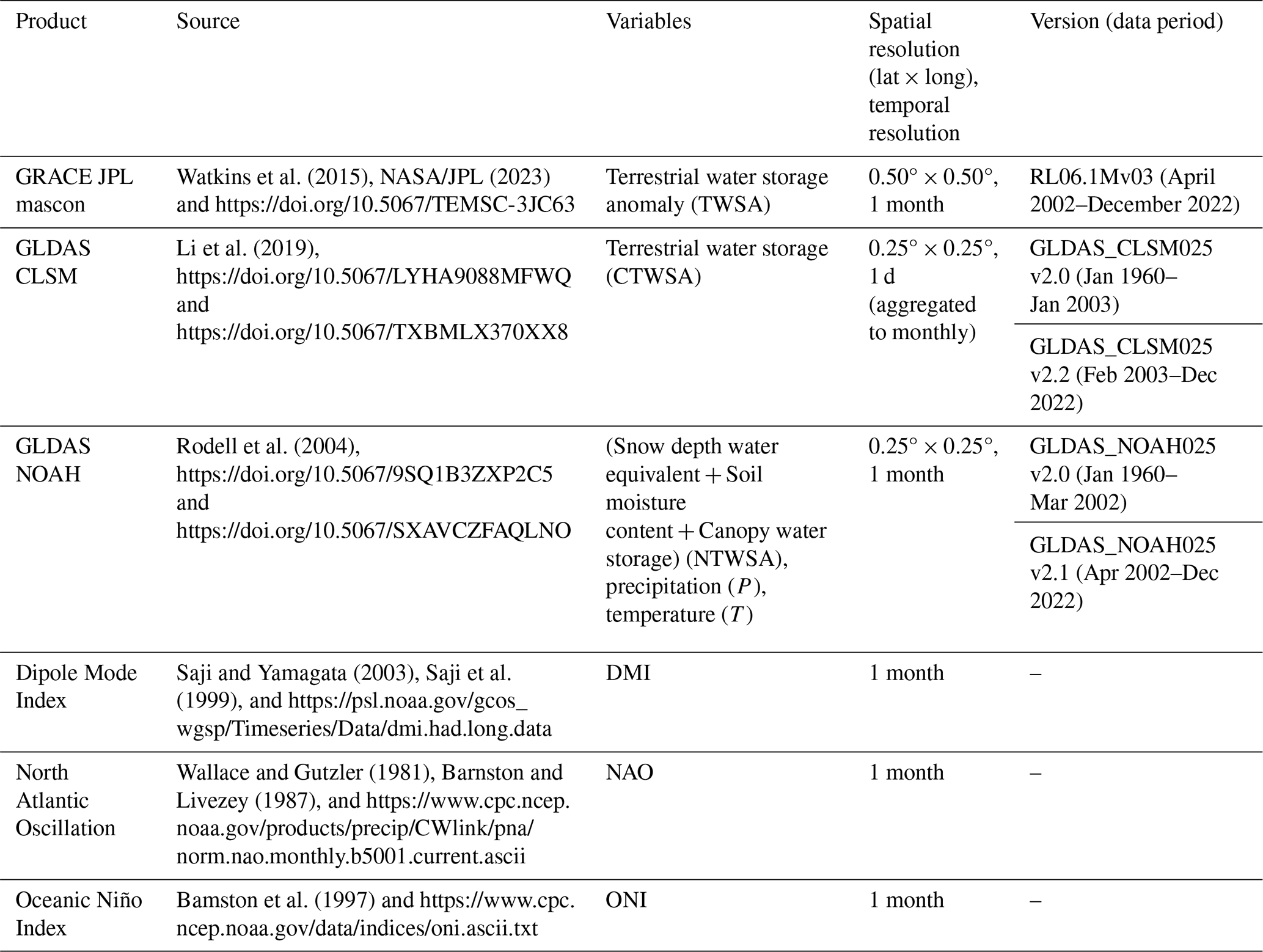
2.3 Meteorological data

Meteorological data, such as precipitation (P) and temperature (T), have been included as predictors to enhance the model's predictive capability. Although precipitation and temperature are components of LSM forcing, the LSM does not utilize all of the data in the forcing to their full potential (Sun et al., 2021). The amount of precipitation affects the recharge of groundwater and surface waters, while temperature is an indicator of the energy available for evapotranspiration. Hence, precipitation and temperature may capture some specific aspect that the LSM models may not simulate accurately (Sun et al., 2019; Humphrey et al., 2017). These climate forcing data (precipitation and temperature) are obtained from GLDAS NOAH LSM output for the period of analysis. These products are selected because of their global coverage and successful usage in earlier investigations (Sun et al., 2019).

2.4 Climate indices

The Dipole Mode Index (DMI), North Atlantic Oscillation (NAO) and Oceanic Niño Index (ONI) have been widely utilized as optimal teleconnection predictors for the seasonality of surface temperature and precipitation (Harou et al., 2006; Brandimarte et al., 2011; Hafez, 2016). DMI is the anomalous SST gradient between the western and southeastern equatorial Indian oceans associated with the Indian Ocean Dipole (Saji et al., 1999; Saji and Yamagata, 2003). The NAO characterizes the changes in strength between the subtropical high-pressure and subpolar low-pressure patterns in the atmosphere over the North Atlantic Ocean (Wallace and Gutzler, 1981; Barnston and Livezey, 1987). The difference between a rolling 3-month average SST in the eastern central tropical Pacific and the long-term average of the same 3 months is characterized as the ONI (Bamston et al., 1997). Recent studies have utilized some climate indices as predictors of TWSAs (Forootan et al., 2019; Phillips et al., 2012; Sun et al., 2021). The prediction skills are spatially impacted by specific climate phenomena or conditions, such as El Niño and La Niña events, represented by those climate indices (Sun et al., 2021).

3 Methodology

As mentioned earlier, TWS from CLSM is obtained directly as one of the outputs (Sun et al., 2021), whereas TWS from NOAH is obtained as the sum of the following components (Sun et al., 2019):

$$\begin{array}{}\text{(1)}& \mathrm{TWS}=\mathrm{SnWE}+\mathrm{SMC}+\mathrm{CWS},\end{array}$$

where SnWE represents snow depth water equivalent, SMC is soil moisture content and CWS is canopy water storage. For both of the aforementioned GLDAS products, the anomalies are computed by subtracting the long-term mean monthly TWS of the period from January 2004 to December 2009 from the monthly TWS values. Let the predictand variable GRACE TWSAs be denoted by t and the set of predictors be denoted by X. Then, the regression problem can be expressed as follows:

$$\begin{array}{}\text{(2)}& t=f(X,p),\end{array}$$

where f represents the regression model and p denotes the model parameter to be solved using $\mathit{\{}{X}_i,t_i{\mathit{\}}}_{i=\mathrm{1}}^N$ as training data; in the latter expression, i=1…N is the index of training sample, and X includes CTWSA, NTWSA, P and T for the current month as well as for 1 and 2 months prior. Additionally, it includes three climate indices (DMI, NAO and ONI) for the current month. In this context, P, P₁ and P₂ represent precipitation for the current month, 1 month prior and 2 months prior, respectively. Four ML algorithms, namely, convolutional neural network (CNN), support vector regression (SVR), extra trees regressor (ETR) and stacking ensemble regression (SER), are trained to solve the regression problem described in Eq. (2). ML models built after training and validation can be used to simulate GRACE-like TWSAs using the inputs only. Figure 1 illustrates the overall workflow adopted in this study. An overview of the predictor selection technique and a brief description of the ML models used in this study are presented in the subsections below.

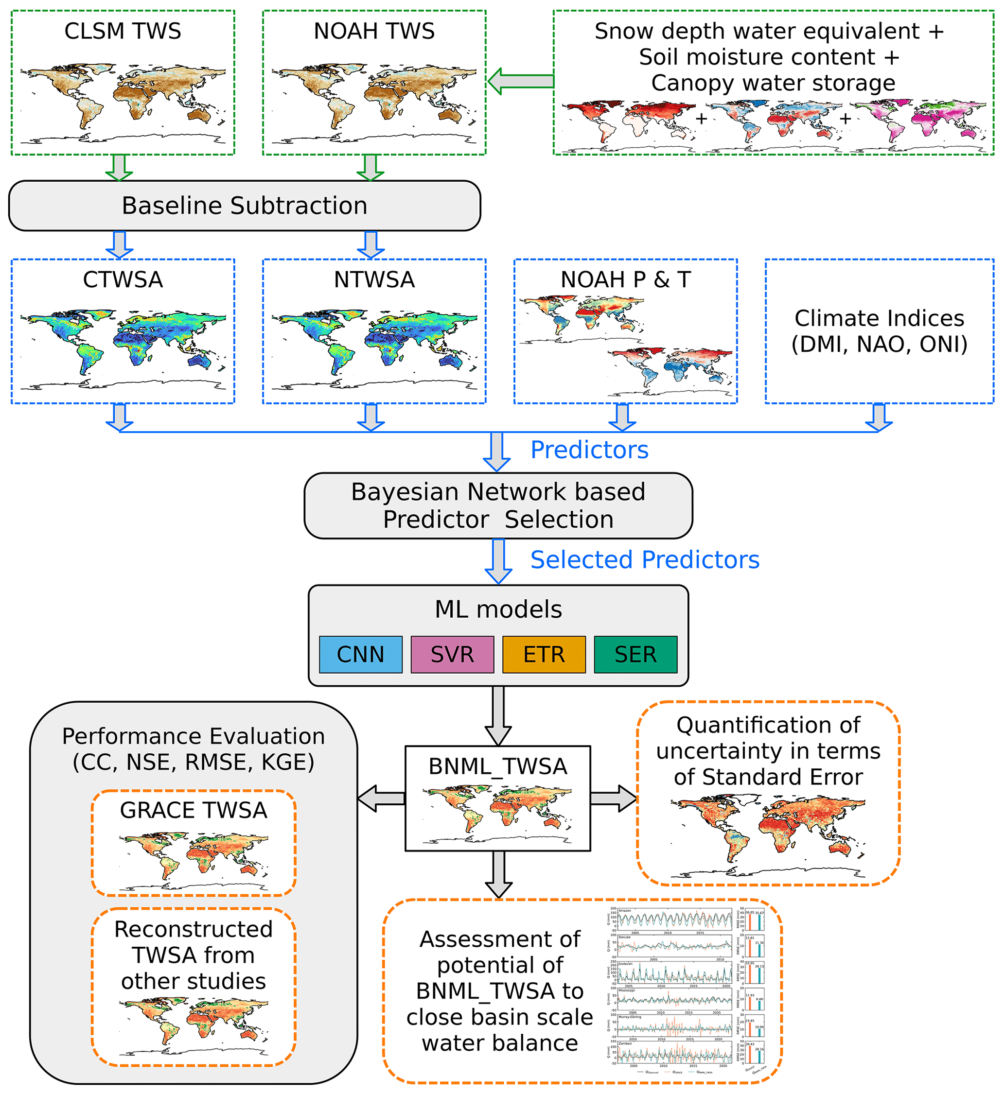
Figure 1 An overview of the methodology employed in this study.

3.1 Predictor selection using Bayesian networks (BNs)

Among the multiple predictors mentioned in the previous section, the most relevant predictors for simulating TWSAs are selected utilizing the potential of Bayesian networks (BNs). The optimal predictors are a subset of all potential predictors of 15 variables. At each grid cell, out of the 15 variables, a subset is selected using BNs, which serves as the “optimum set of predictors” for that grid cell. The optimum set of predictors are selected based on probabilistic independence–dependence structure. BNs serve as compact representations of probabilistic relationships among a defined collection of random variables (Das and Chanda, 2022). These networks are characterized by a graph $G=(V,E)$, where each vertex (node) vϵV corresponds to one of the aforementioned random variables in X. Through edges (arcs) eϵE, the network articulates the conditional independencies or dependencies that exist among the variables within X, collectively termed the graph's dependence structure. This framework employs directed acyclic graphs (DAGs) to concisely encapsulate probabilistic relations and effectively portray the joint distribution of the variables (Scutari and Nagarajan, 2011). In the context of a DAG, the inclusion of arcs may or may not indicate a causal relationship between variables where one variable can be understood as the cause and the other as the effect (Sevinc et al., 2020). When an edge connects two nodes in the graph, the node from which the edge originates is referred to as the parent node, while the node where the edge terminates is known as the child node. The process of determining the topology of the graph G is termed structure learning. This involves identifying the graph structure that effectively represents the conditional independencies observed within the data. Several algorithms have been presented in the literature to tackle this problem, and they are broadly classified into three categories: constraint-based algorithms (which are based on conditional independence tests), score-based algorithms (which are based on goodness-of-fit scores) and hybrid algorithms (which combine the previous two approaches). In the realm of continuous variables, score-based algorithms have outperformed their constraint-based counterparts in terms of performance. The challenge with constraint-based algorithms lies in their tendency to yield partially directed acyclic graphs (PDAG), which can subsequently disrupt precise predictions for the target variable (Das and Chanda, 2020).

Score-based learning offers both precise and approximate solutions. Precise solutions ensure the identification of the graph that optimizes an objective function while adhering to a maximum in-degree constraint (Constantinou et al., 2021). These algorithms, also referred to as search-and-score algorithms, involve the utilization of heuristic optimization methods to tackle the task of acquiring the structure of a BN. In this process, each potential network configuration is assigned a score that indicates its goodness of fit, and the objective of the algorithm is to maximize this score. The hill-climbing (HC) algorithm, a classical heuristic search algorithm, has been the major choice for this purpose in most of the hydrology-related studies (Vitolo et al., 2018; Das and Chanda, 2022, 2020; Dutta and Maity, 2021; Chanda and Das, 2022).

The HC algorithm commences its process with an initial empty graph and systematically explores potential DAGs to maximize the network's score, achieved through operations like adding, removing or reversing arcs, determined by the strength of edges (Scutari and Denis, 2021). The network's score is calculated using the Bayesian information criteria (BIC) to prevent overfitting, wherein the BIC score is determined by a formula incorporating the number of parameters in the global distribution (“d”) and the dataset length (“N”). A critical concept within the HC algorithm is edge strength, reflecting the disparity in the BIC score when a specific arc is included or excluded, indicating the degree of interdependency between connected nodes. A higher edge strength signifies a stronger correlation. In essence, the HC algorithm employs an iterative approach, optimizing the network score by manipulating the DAG's structure based on edge strengths determined through the BIC score, thereby striking a balance between model complexity and data fidelity while also emphasizing significant node interconnections. The BIC score formula is given by the following expression:

$$\begin{array}{}\text{(3)}& \mathrm{BIC}=\sum _{i=\mathrm{1}}^N\log \left(\mathit{Pr}\left(X_i\right|\mathrm{MB}\left(X_i\right))\right)-{\displaystyle \frac{d}{\mathrm{2}}}\log \left(N\right),\end{array}$$

where MB represents the Markov blanket, which is the minimal set of nodes that can predict a target node. The bnlearn package in the R environment (Scutari, 2010) is used to develop the DAG networks.

3.2 Machine learning algorithms for TWSA modeling

This section presents a concise overview of ML algorithms used to model TWSAs. In this study, four types of ML algorithms have been used: neural network-based algorithms (CNN), kernel-based algorithms (SVR), tree-based algorithms (ETR) and an ensemble of these three (CNN, SVR and ETR) as stacking ensemble regression (SER).

3.2.1 Convolutional neural networks (CNNs)

CNNs belong to a category of neural networks particularly well suited to handling data with grid-like structures, such as images or time-series data. The primary advantage that they offer over conventional feed-forward neural networks is their utilization of mathematical linear operations, known as convolutions (Uz et al., 2022). These layers possess the capability to autonomously extract features, identifying crucial aspects within the input data that are essential for establishing the correlation between input and output variables. Hence, CNNs have the capacity to manage raw data and are devoid of the necessity to preprocess or manually extract features (Ferreira and da Cunha, 2020). CNNs find widespread application in image recognition tasks. For images, which possess two dimensions, convolutional filters of corresponding dimensions are employed. Conversely, for tasks involving sequential data or time series, like the context of this study, CNNs with one-dimensional (1D) convolutional filters (1D-CNNs) are employed. In this study, a 1D-CNN comprises a single convolutional layer and two fully connected layers. The activation function “ReLU” is applied within the convolutional layer (Ferreira and da Cunha, 2020; Alibabaei et al., 2021; Ahmed et al., 2022). To mitigate overfitting, a dropout layer is introduced following each convolutional layer. The training algorithm employed for this model is Adam. The learning rate is established at 0.1, and the number of training epochs is determined using early stopping, with a maximum limit of 200 epochs. Additionally, the batch size is configured to 32.

3.2.2 Support vector regression (SVR)

Support vector regression (SVR) is a pivotal component of support vector machines (SVMs), an algorithm introduced by Cortes and Vapnik (1995), designed to handle nonlinear regression problems. SVR extends the fundamental concept of SVMs by effectively addressing regression tasks through a nonlinear mapping of input data into a higher-dimensional feature space. The underlying principle of SVR is based on the concept of the “kernel trick”. This technique employs a kernel function, such as the radial basis function (RBF) kernel, to transform the input data into a feature space where linear regression can be applied effectively. The kernel function aids in defining a hyperplane – a decision boundary – within this feature space. This hyperplane facilitates the prediction of target values by distinguishing between different types of data patterns. Moreover, SVR aims to establish a boundary layer at a certain distance from the hyperplane, enclosing the data points that lie proximate to the hyperplane, known as support vectors. Selecting an appropriate kernel function is a crucial step in SVR. Raghavendra and Deka (2014) highlight that polynomial and RBF kernels are commonly employed for nonlinear problems. However, Das and Chanda (2020) advocate for the superiority of the RBF kernel in nonlinear regression tasks, leading to its preference. For a more comprehensive understanding of the algorithms employed in this context, detailed insights and further elucidation can be gleaned from the work of Raghavendra and Deka (2014), Das and Chanda (2020), and Das et al. (2022).

3.2.3 Extra trees regressor (ETR)

In the realm of ensemble-based predictive modeling, the ETR shares a fundamental principle that is built on the foundation of decision trees and random forests, combining their strengths to create an ensemble of diverse decision trees, and is less likely to overfit a dataset (Ahmad et al., 2018). In the ETR framework, a random subset of features is employed to train each individual base estimator, akin to the approach used in random forest, where all of the predictors are employed. This attribute ensures diversity among the constituent trees, contributing to the model's generalization capabilities and mitigating the risk of overfitting. While random forest selects the optimal feature from the random subset to split a node, ETR takes this a step further by introducing an additional layer of randomness (Kumar et al., 2022). ETR not only randomly selects a feature from the subset but also stochastically chooses the corresponding split value for the chosen feature. This distinctive feature selection strategy imparts an extra level of variance to the model, rendering it more robust and capable of capturing intricate relationships in the data (Ahmad et al., 2018). The predictions of the individual trees are combined to generate the ultimate prediction through a process of arithmetic averaging. The algorithm is influenced by two pivotal parameters: the count of predictors chosen randomly at each node and the minimum sample size required to initiate a node split (Sun et al., 2021).

3.2.4 Stacking ensemble regression (SER)

Stacking, a form of meta-learning, aims to enhance predictive performance by combining predictions from multiple base models through a higher-level integrated model (Zounemat-Kermani et al., 2021). The stacking generalization framework presents a couple of avenues for maximizing predictive gains. One approach involves employing diverse base learners, thereby fostering variability among the base models. Alternatively, enhancing the ensemble size while keeping the number of base learners constant can also provide the meta-learner with a broader range of insights. In this context, the term “meta-learner” refers to an aggregating model that learns the optimal way to combine outputs from the base learners. These “base learners” constitute the models whose individual predictions are assembled in the final step (Lee and Ahn, 2021). To mitigate overfitting, out-of-sample data are employed for training the meta-model. This entails utilizing predictions from the base learners on this external data. The overarching objective is for the meta-model to establish an optimal correlation between observed values and its own predictions. The process is aptly termed “stacking”, as it involves merging predictions from validation sets, thereby creating a fresh dataset for the meta-model to glean insights from. Additional valuable insights can be obtained from the comprehensive analysis of ensemble ML presented in the review of Martinez-Gil (2022), Zounemat-Kermani et al. (2021), and Lee and Ahn (2021). In the present study, CNN, SVR and ETR are used as the base models. During the training process, initial predictions are first generated by the base learners. Subsequently, these predictions from the base learners serve as inputs to the meta-learner, which produces the ultimate output. While all base models are utilized as potential meta-models to assess overall accuracy, preference is given to the generalized linear model (GLM) due to its superior effectiveness as a meta-learner compared to the alternative models.

3.3 Training and performance evaluation

The period of observed GRACE data used in this study is from April 2002 to December 2022 (216 months in total excluding the GRACE data gaps). Within this period, the available months from 2010 to 2016 (68 months) are used as the testing period, whereas the remaining portion of the dataset (148 months) is used to train the ML models. The 5-fold cross-validation technique is employed during the training phase to address the issue of insufficient data length. Additionally, all input parameters for the ML models have been normalized within the range of 0 to 1. The simulated TWSAs employing BNs as the optimal predictor selector in conjunction with various ML models are henceforth referred to as BNML_TWSA. The performance of the BNML_TWSA from each of the models is evaluated against GRACE/GRACE-FO TWSAs using several agreement metrics, including the Pearson correlation coefficient (CC), the Nash–Sutcliffe efficiency (NSE) coefficient, the root-mean-square error (RMSE) and the Kling–Gupta efficiency (KGE). The CC is calculated as follows:

$$\begin{array}{}\text{(4)}& \mathrm{CC}={\displaystyle \frac{{\sum }_{i=\mathrm{1}}^n(O_i-\stackrel{\mathrm{‾}}{O})(S_i-\stackrel{\mathrm{‾}}{S})}{\sqrt{{\sum }_{i=\mathrm{1}}^n(O_i-\stackrel{\mathrm{‾}}{O}{)}^{\mathrm{2}}}\sqrt{{\sum }_{i=\mathrm{1}}^n(S_i-\stackrel{\mathrm{‾}}{S}{)}^{\mathrm{2}}}}},\mathrm{CC}\in [-\mathrm{1},\mathrm{1}],\end{array}$$

where O_i and S_i represent the TWSAs from GRACE/GRACE-FO and the simulated/reconstructed TWSAs, respectively, with $\stackrel{\mathrm{‾}}{O}$ and $\stackrel{\mathrm{‾}}{S}$ denoting their respective means.

The other three metrics are expressed as follows:

$$\begin{array}{}\text{(5)}& {\displaystyle }\mathrm{NSE}=\mathrm{1}-{\displaystyle \frac{\sum _{i=\mathrm{1}}^n(O_i-S_i{)}^{\mathrm{2}}}{\sum _{i=\mathrm{1}}^n(O_i-\stackrel{\mathrm{‾}}{O}{)}^{\mathrm{2}}}},\mathrm{NSE}\in (-\mathrm{\infty },\mathrm{1}],\text{(6)}& {\displaystyle }\mathrm{RMSE}=\sqrt{{\displaystyle \frac{\mathrm{1}}{n}}\sum _{i=\mathrm{1}}^n(O_i-S_i{)}^{\mathrm{2}}},\mathrm{RMSE}\in [\mathrm{0},+\mathrm{\infty }),\text{(7)}& {\displaystyle }\begin{array}{rl}\mathrm{KGE}& =\mathrm{1}-\sqrt{(\mathrm{CC}-\mathrm{1}{)}^{\mathrm{2}}+{\left({\displaystyle \frac{\stackrel{\mathrm{‾}}{S}}{\stackrel{\mathrm{‾}}{O}}}-\mathrm{1}\right)}^{\mathrm{2}}+{\left({\displaystyle \frac{{\mathit{\sigma }}_{\mathrm{S}}}{{\mathit{\sigma }}_{\mathrm{O}}}}-\mathrm{1}\right)}^{\mathrm{2}}},\\ & \mathrm{KGE}\in (-\mathrm{\infty },\mathrm{1}].\end{array}\end{array}$$

Here, σ_O is the standard deviation in observations and σ_S the standard deviation in simulations. The size of the test sample is denoted by n. A higher value for CC, NSE and KGE, closer to 1, and a lower value for RMSE, closer to 0, indicate superior performance (Nash and Sutcliffe, 1970; Gupta et al., 2009).

4 Results and discussion

4.1 Selected predictors using BNs

The optimal predictors for each grid cell across the globe (58 027 grid cells in total) are selected using BNs. For each predictor, the spatial map showing the grid cells where they are selected by the BNs as optimal predictors is depicted in Fig. 2. Figure 2 also shows a bar plot with the number of grid cells where each predictor is retained by the BN. CTWSA is selected by the BN as an optimal predictor for the maximum number of grid cells (71.06 %), followed by ONI (56.03 %) and NTWSA (48.71 %). The selection of CTWSA as the best predictor of GRACE TWSAs is also suggested by other studies conducted in different regions around the globe (Sun et al., 2021). Among the 11 global river basins specifically investigated in this study, the number of grid cells with CTWSA as an optimal predictor is lower in the Amazon and Nile basins compared to the other basins. Only 3.55 % of the total grid cells hold the NAO as an optimal predictor as selected by the BNs. This is reflected at the river basin scale as well; for each of the river basins, a very limited percentage of grid cells retain the NAO as an optimal predictor. It is noteworthy that, in addition to TWSAs from LSMs, the ONI and DMI have been selected as optimal predictors for a substantial number of grid cells. Meteorological variables such as P and T, along with their observations from previous months, have been selected for fewer grid cells globally by the BN compared to ONI and DMI. This can be attributed to the fact that LSMs already incorporate these meteorological variables as forcing inputs. The inclusion of climate indices as potential predictors for a large number of grid cells can be seen as an effort to represent the climate change scenarios of that specific time period. In a limited number of grid cells (66), the BN did not select any predictors. For an additional 492 grid cells, the BN selected only one predictor, thereby limiting the application of certain ML algorithms to these grid cells. Consequently, for a total of 558 grid cells, which constitute less than 1 % of the grid cells considered in this study, the complete set of 15 predictors has been used as potential predictors.

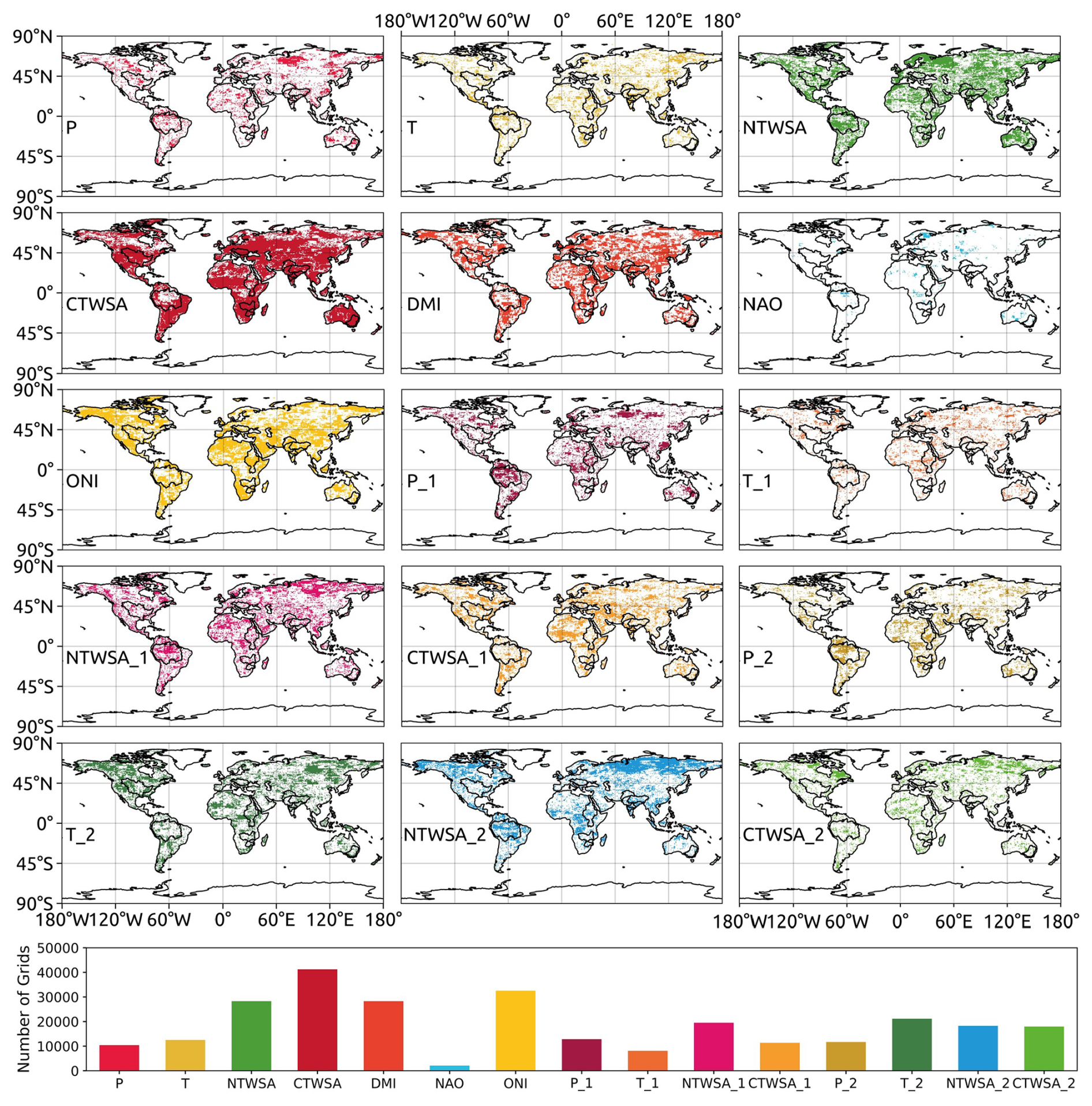
Figure 2 Spatial distribution and bar plot of selected predictors using a Bayesian network. P, P₁ and P₂ represent precipitation for the current month, 1 month prior and 2 months prior, respectively. Similarly, T, NTWSA and CTWSA, along with their observations 1 month prior and 2 months prior, are used as potential predictors. T denotes temperature, while TWSAs from NOAH and the Catchment Land Surface Model (CLSM) are denoted using NTWSA and CTWSA, respectively.

4.2 Grid-cell-specific leader models

The predictors selected by the BNs at each grid cell are employed as input to predict the TWSAs using the four ML algorithms mentioned earlier: CNN, SVR, ETR and SER. The grid-cell-wise leader ML algorithm is identified based on the Pearson correlation coefficient (CC) between predicted TWSAs and GRACE TWSAs for the test period. The performance difference between the leading ML algorithm and the worst-performing ML model is depicted in Fig. 3. Grid cells that have negative CC values (∼2.65 % of the total grid cells considered in this study) for the leading ML model have been excluded when calculating the difference. Although the improvement in terms of the CC value difference is not large for all grid cells globally, more than 14.4 % of grid cells show improvements greater than 0.2, while an additional 15.7 % of grid cells exhibit improvements of between 0.1 and 0.2. A grid cell exhibiting the maximum improvement within the basins considered in this study has been selected to demonstrate this improvement. The time series and scatterplot are illustrated in Fig. 4. The estimated TWSAs by the best-performing model are in good agreement with the observed TWSAs during the testing period. This justifies the use of the best-performing (leading) model to predict the TWSAs. Figure 5 depicts the spatial distribution of the leader algorithms over the globe along with the frequency as a bar plot. ETR performs the best for the maximum number of grid cells, with a total of 25 703, followed by SVR, SER and CNN, which perform best for 11 609, 11 069 and 9646 grid cells, respectively. Thus, for most of the river basins (including the Krishna and Godavari in India; the Danube in Europe; the Nile, Zambezi and Limpopo on the African continent; the Mississippi in the USA; and the transboundary GBM and Indus), ETR emerges as the leader model in the maximum number of grid cells. The contribution of the leader algorithm as a percentage of the total grid cells for each river basin is shown in Fig. 5c. In the Limpopo Basin, it is observed that ETR performs best in 89.0 % of the grid cells, whereas CNN does not perform best in any of the grid cells in this basin. In the Murray–Darling Basin in Australia, the four ML algorithms show the best performance in an approximately equal number of grid cells (CNN: 25.9 %; SVR: 21.4 %; ETR: 26.1 %; SER: 26.6 %).

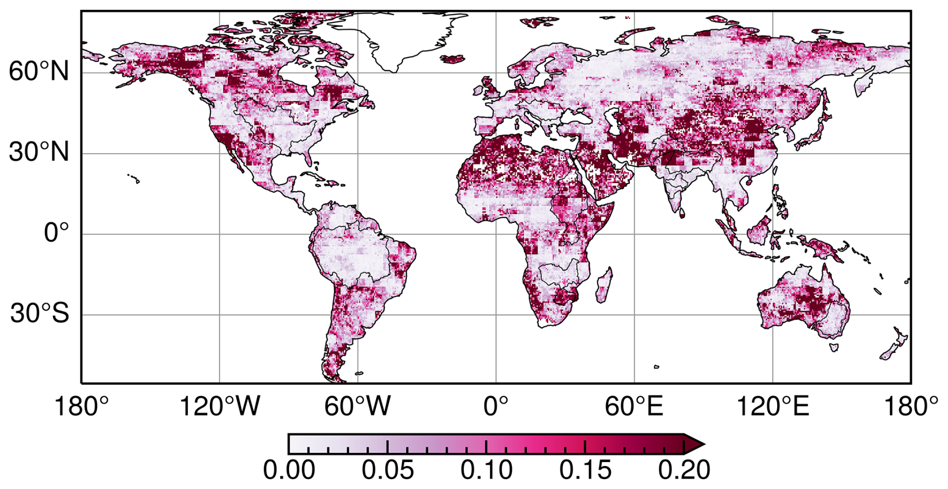
Figure 3 Difference between the correlation coefficient (CC) values obtained from the leader ML model (excluding negative CC values) and the worst-performing ML algorithm at each grid cell during the test period.

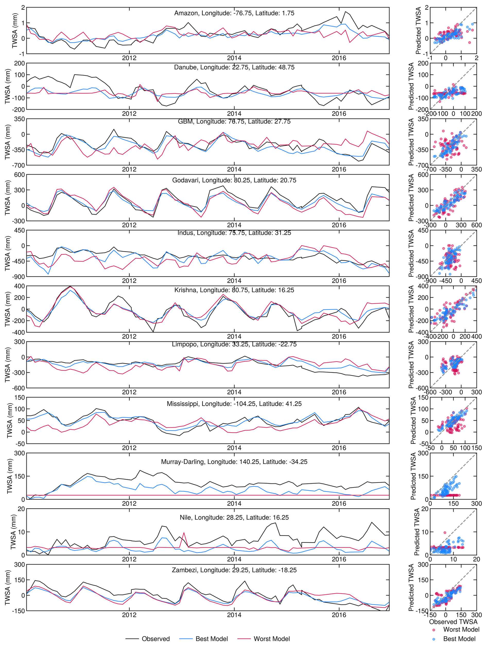
Figure 4 Time series (left columns) for grid cells showing the maximum improvement within the basins considered in this study, including observed TWSAs and TWSAs predicted by the best and worst models. Scatterplots (right columns) compare the TWSAs predicted by the best and worst models with the observed TWSAs.

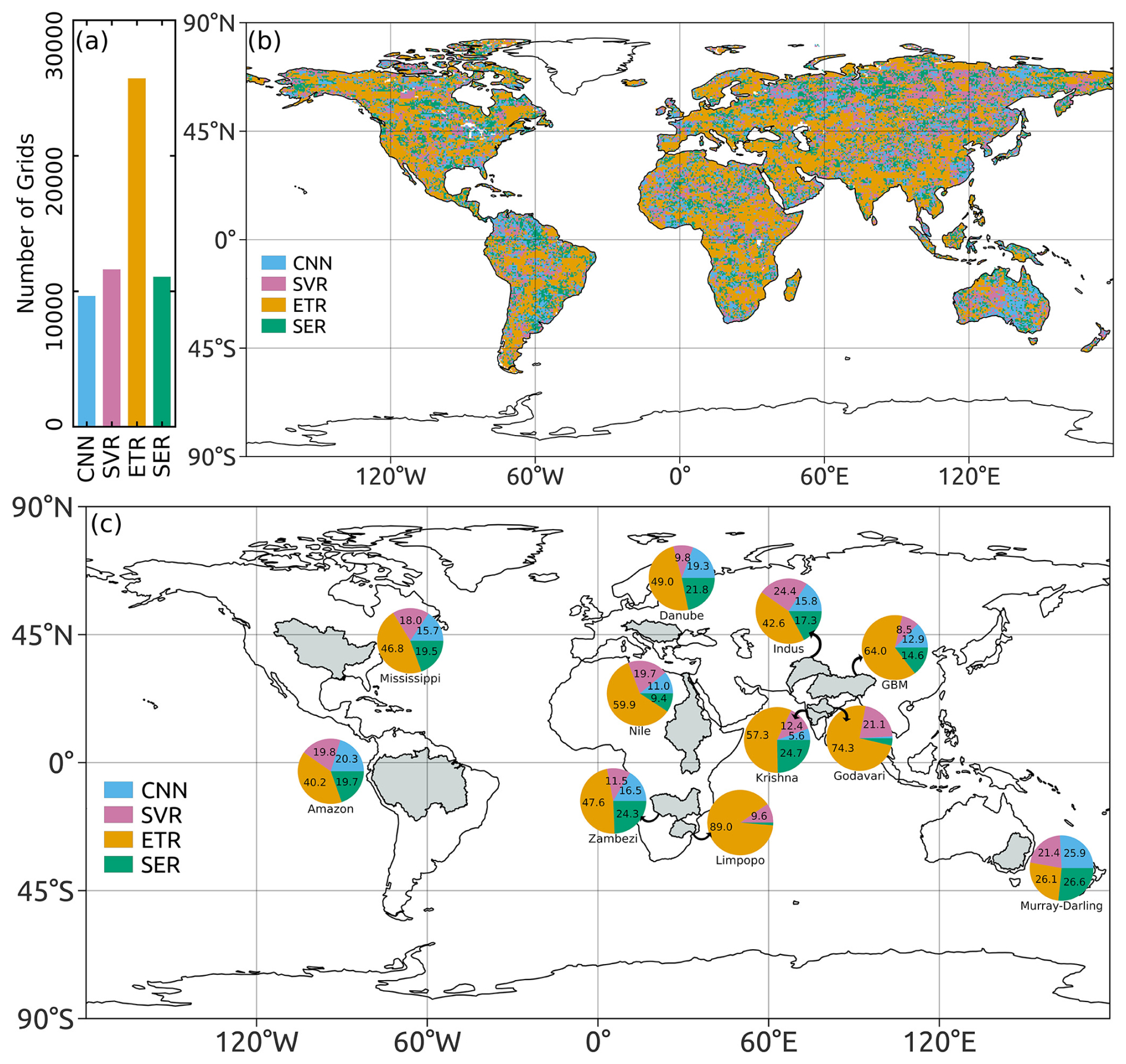
Figure 5 (a) Frequency, (b) spatial distribution of leader ML algorithms and (c) leader ML algorithms in terms of percentage for different river basins.

4.3 Performance evaluation of simulated global BNML_TWSA

For the leader ML models at each grid cell, the BNML_TWSA is evaluated against the GRACE TWSAs during the testing period (68 months). Performance measures, such as the CC, NSE, RMSE and KGE, are computed for the BNML_TWSA at both the basin-wide and grid cell levels. Similar performance measures are also computed for CTWSA and NTWSA. The spatial distribution of CC, NSE and KGE obtained from NTWSA, CTWSA and the BNML_TWSA using the identified leader ML models during the test period is shown in Fig. 6. According to Fig. 6a and d, it is evident that the agreement between CTWSA and GRACE TWSAs is better than that of NTWSA. However, the BNML_TWSA (as shown in Fig. 6g) performs better in most grid cells worldwide compared to the TWSAs obtained from the LSMs (CTWSA and NTWSA). The BNML_TWSA showed clear improvement in performance over NTWSA and even CTWSA in all of the basins, except for the western part of the Nile Basin and the southwestern part of the Mississippi Basin where CTWSA shows a closer match with the GRACE TWSAs in some grid cells. The cumulative distribution functions (CDFs) of the CC, NSE and KGE metrics are presented in Fig. 7. These CDFs demonstrate that BNML_TWSA exhibits significantly superior performance, characterized by substantially higher CC, NSE and KGE values. As shown by the BNML_TWSA results, the arid, semiarid and certain wet regions (e.g., the arid desert part of the Nile Basin, the semiarid regions of the Mississippi Basin and parts of the Congo Basin) have poorer model performance, which is consistent with other global studies (Mo et al., 2022). A substantial improvement in the performance by the proposed model can be observed in most parts of India, eastern Europe and South America. Figure 6b, e and h depict the NSE values obtained from NTWSA, CTWSA and the BNML_TWSA, respectively. Similarly, Fig. 6c, f, and i present the spatial distribution of KGE values for NTWSA, CTWSA and BNML_TWSA across the globe. The results indicate the superior performance of BNML_TWSA compared to the other methods, which is evident from these plots at a global scale.

The grid-cell-wise CC, NSE, RMSE and KGE values are further compared for the three TWSA datasets (NTWSA, CTWSA and BNML_TWSA) in all river basins as box plots depicted in Fig. 8. The median values of each matrix are listed in Table 2. For most of the basins, BNML_TWSA shows a higher median value of CC and a smaller range in the box plot compared to NTWSA and CTWSA, indicating a better performance for the proposed BNML_TWSA. However, for the Indus, Limpopo, Nile and Zambezi basins, CTWSA has a slightly better performance than BNML_TWSA. All of the grid cells in the Amazon, Danube, Godavari, Krishna, Mississippi and Zambezi basins have a CC value of ≥0.75 for BNML_TWSA. Similarly, for the GBM and Murray–Darling basins, the lowest CC value among all grid cells is above 0.5. The NSE, which compares the residual variance (the “noise”) with the variance in the measured data, shows poor results (<0) for most of the basins for both NTWSA and CTWSA. On the other hand, the NSE values for BNML_TWSA are fairly high (>0.68) in most basins, except for the Indus, Limpopo, Murray–Darling and Nile, and only the Indus Basin has a median NSE value of less than 0. Hence, based on the NSE value, BNML_TWSA has better performance than NTWSA and CTWSA for all of the river basins. The improved performance of BNML_TWSA can also be illustrated by the distribution of the RMSE values over each river basin, depicted in Fig. 8. When comparing the overall spread of the RMSE values for BNML_TWSA, CTWSA and NTWSA, it is observed that the range of the RMSE values for BNML_TWSA is lower than that of CTWSA and NTWSA. This indicates that the interquartile range (IQR), the difference between the third quartile and the first quartile, of the RMSE values for BNML_TWSA is smaller than that of CTWSA and NTWSA. Similarly, the KGE values indicate that CTWSA exhibits the best performance in the Godavari Basin. For all other basins, BNML_TWSA shows superior performance.

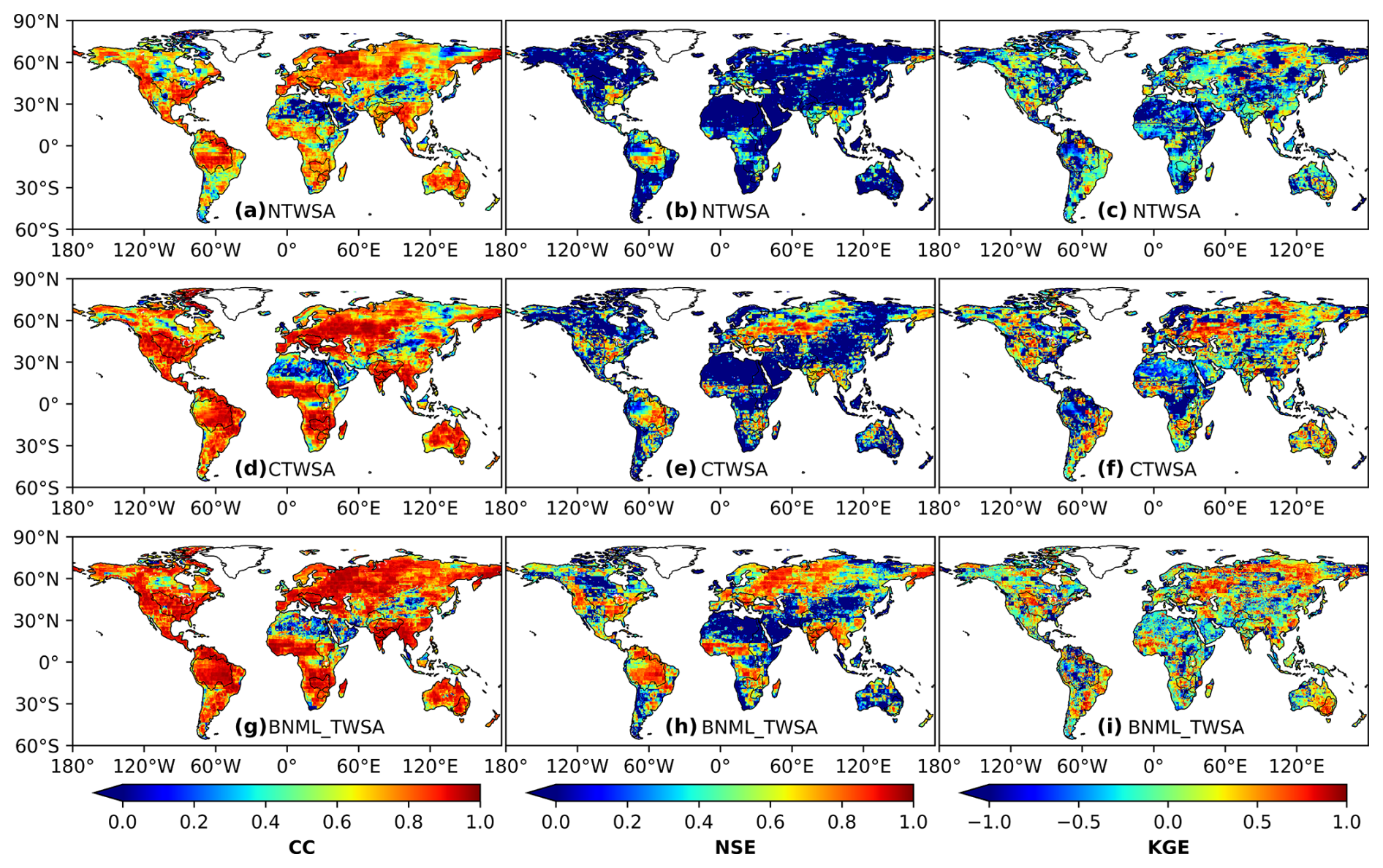
Figure 6 Correlation coefficient (CC), Nash–Sutcliffe efficiency (NSE) coefficient and Kling–Gupta efficiency (KGE) values between observed GRACE TWSAs and NTWSA, CTWSA and BNML_TWSA.

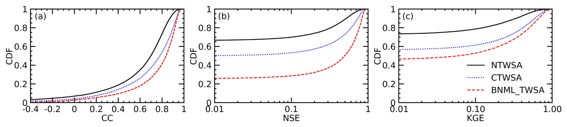
Figure 7 Cumulative distribution functions (CDFs) of the correlation coefficient (CC), Nash–Sutcliffe efficiency (NSE) coefficient and Kling–Gupta efficiency (KGE) values, as depicted in Fig. 6.

Table 2 Median of the CC, NSE, RMSE and KGE values at grid cells of each basin. A bold value signifies the best performance.

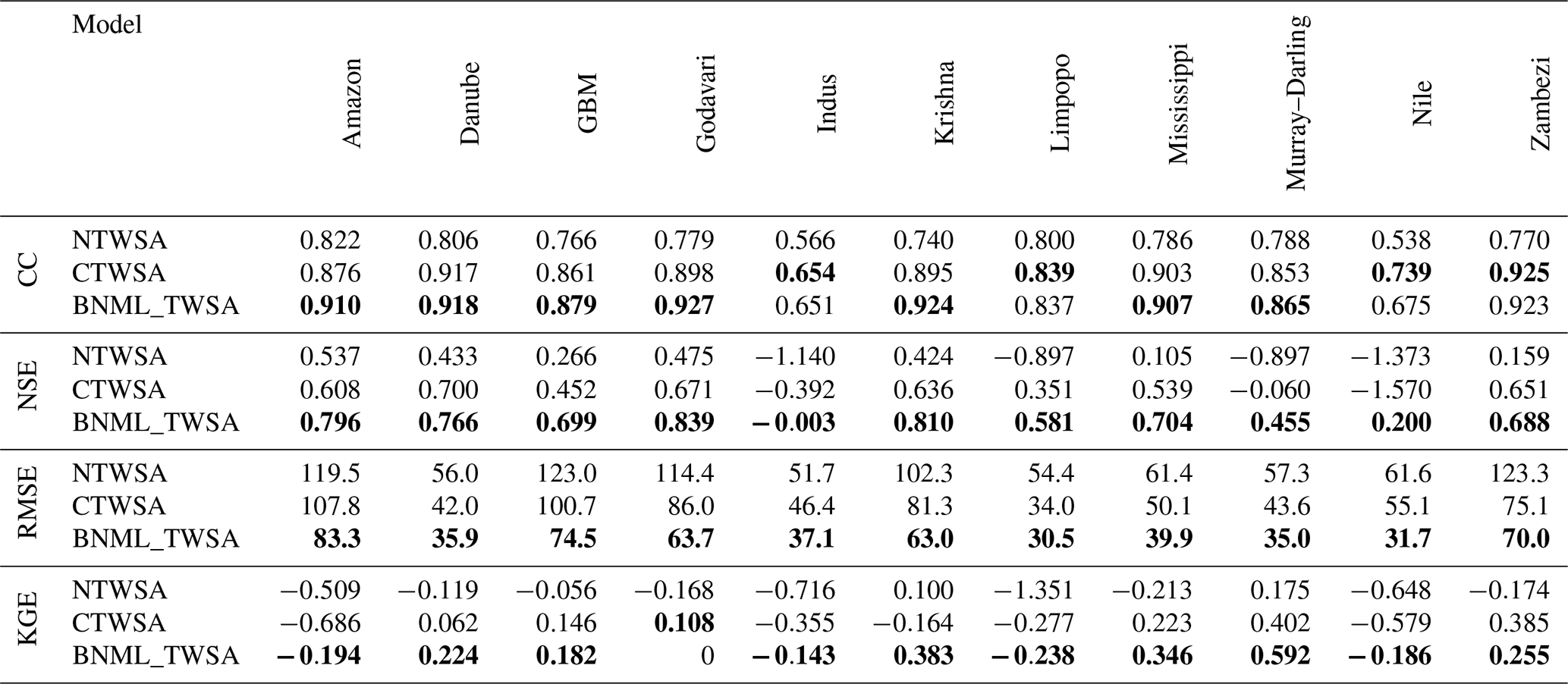
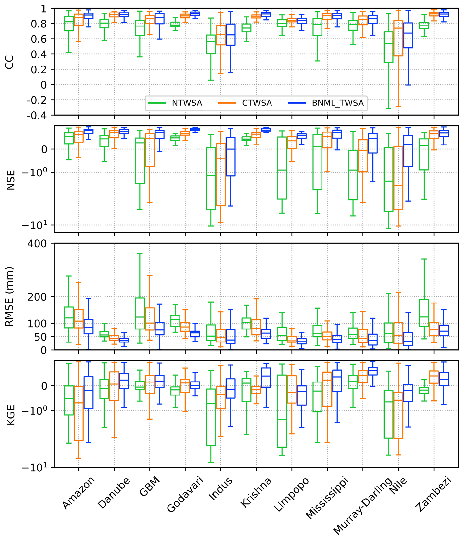
Figure 8 Box plot of CC, NSE, RMSE and KGE values for the grid cells of each basin, excluding the outliers.

4.4 Basin-scale quality assessment of gap-filled TWSAs

The results presented in the preceding sections demonstrate the superior ability of the proposed model to simulate GRACE TWSAs during the testing period. The leader model, constructed for each global grid cell, is utilized to generate a GRACE-like TWSA series from April 2002 to December 2022 using the input parameter set selected by the BNs for each grid cell. Figure 9 shows the time series of average reconstructed TWSAs for all grid cells within a river basin. TWSAs from GLDAS NOAH (NTWSA), GLDAS CLSM (CTWSA) and GRACE are also included in Fig. 9 for comparison. The seasonal variation in TWSAs is greatly captured by the proposed models and the other two LSM outputs. Similar to observations from previous sections, the CTWSA has better performance than the NTWSA. However, even better performance is achieved by the proposed BNML_TWSA. Compared to the observed GRACE TWSAs, both NTWSA and CTWSA underestimate the peak values of TWSAs for the Amazon Basin, whereas the BNML_TWSA time series matches the GRACE TWSAs most closely. For the Indus and Nile river basins, the mismatch between GRACE TWSAs and TWSAs from LSM outputs has been widening since 2010; however, the proposed model simulates BNML_TWSA, which is very close to the GRACE TWSAs.

The basin-wise performance of the mean BNML_TWSA and CTWSA is assessed against the GRACE TWSAs and depicted as a scatterplot in Fig. 10. NTWSA is not included in this plot, as it has already been found to be a poorer match with GRACE TWSAs than the CTWSA. The CC of BNML_TWSA in the Zambezi Basin is the highest among all of the basins (0.989); however, the RMSE (46.1 mm) and NSE (0.833) values do not suggest that its performance is the best. The basin-wide mean BNML_TWSA has a higher CC (≥0.904) than CTWSA for the GBM, Godavari, Indus, Krishna, Limpopo, Mississippi, Murray–Darling and Zambezi basins (see Fig. 10). In the Nile Basin, a high CC value of 0.82 is obtained for BNML_TWSA; however, this is the minimum among all river basins. The Nile Basin is one of the few basins where CTWSA has a slightly higher CC (0.889) than BNML_TWSA (see Fig. 10), but the time-series plot (see Fig. 9) shows that the BNML_TWSA is in better agreement with GRACE TWSAs. This indicates that, in general, the proposed BNML_TWSA is more reliable than CTWSA. Considering the NSE and RMSE values, the Amazon, GBM, Godavari, Krishna and Nile basins perform better with BNML_TWSA than with CTWSA. The only exception is Danube Basin which has a marginally lower performance for BNML_TWSA than CTWSA according to the basin-wide mean. However, when considering the KGE values, BNML_TWSA outperforms CTWSA in most basins. With the exception of the Danube, Indus, Krishna, Murray–Darling and Zambezi basins, all other basins demonstrate superior performance for BNML_TWSA compared to CTWSA when evaluated using the KGE values.

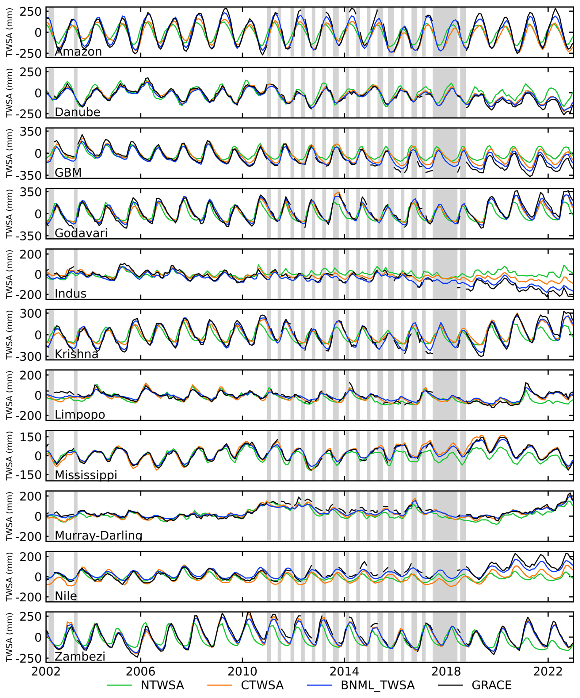
Figure 9 Comparison of TWSA time series from April 2002 to December 2022 (GRACE period). Vertical gray bars indicate missing GRACE observations.

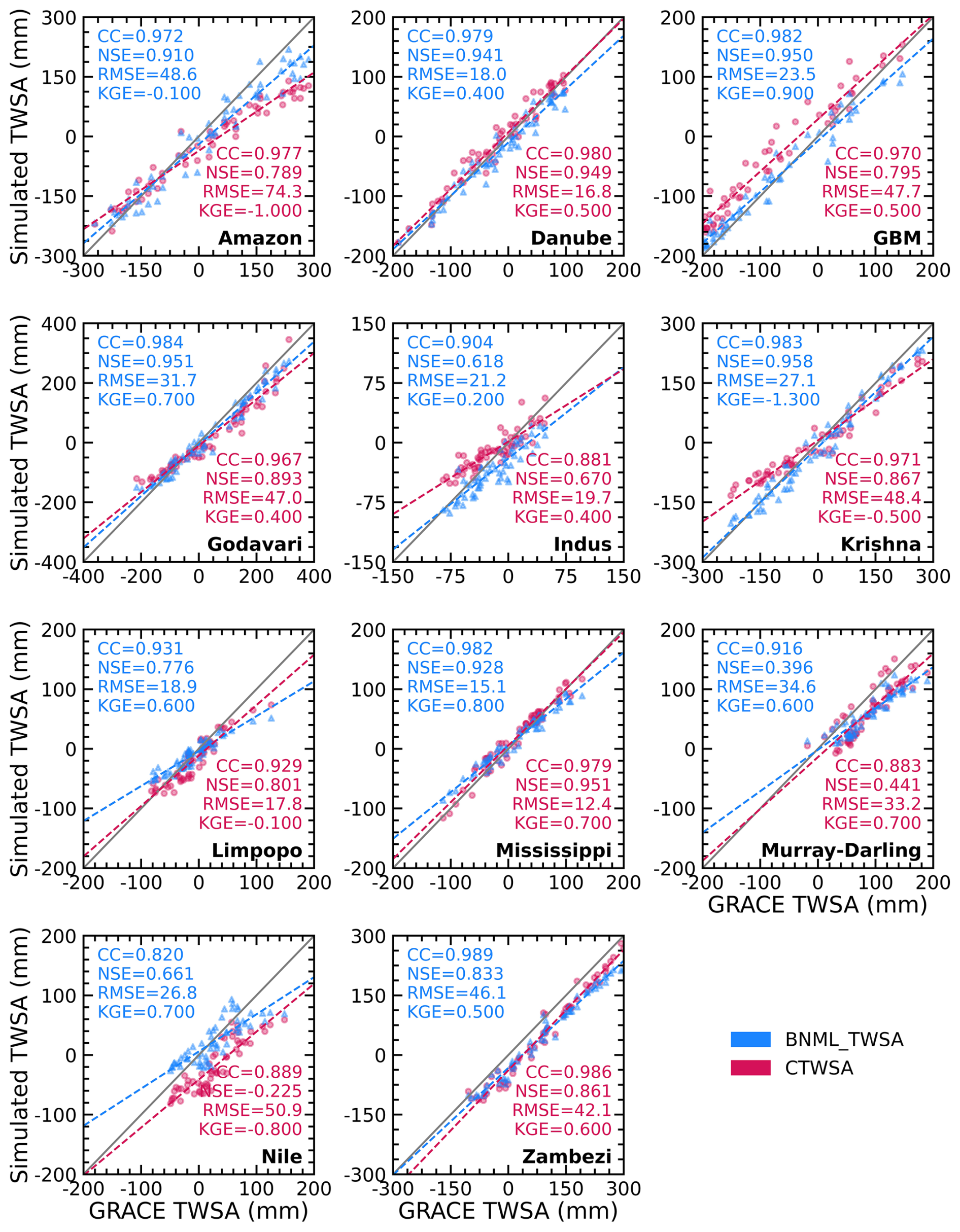
Figure 10 Scatterplot of the basin-wise mean of observed GRACE TWSA vs. BNML_TWSA and CTWSA for each river basin.

4.5 Reflection of hydroclimatic extreme events in BNML_TWSA during the pre-GRACE (1960–2002) and intermediate gap periods

The leader ML model of each grid cell is used to hindcast BNML_TWSA during the pre-GRACE period (January 1960–March 2002) using the predictors selected by BNs. The basin-averaged BNML_TWSA series is shown in Fig. 11. Similar to the LSM outputs (CTWSA and NTWSA), increasing and decreasing trends are noted for BNML_TWSA series for some of the river basins. The variability in the TWSA hindcast is lowest for the Indus (−95.1 to 75.4 mm) and Limpopo (−61.6 to 83.7 mm) river basins, while the Amazon (−227.5 to 199.6 mm) and Krishna (−200.7 to 239.5 mm) basins have the highest variability. The minimum TWSA hindcast values for the Murray–Darling and Nile basins are around −20 mm – the lowest among all of the regions. During this hindcast period, a number of significant extreme climate events occurred; for example, two severe flood events in India are depicted in Fig. 12a–b. First, the Gomti River, a tributary of the Ganges River, overflowed and caused a severe flood that inundated half of the city of Lucknow in mid-October 1960. As shown in Fig. 12a, water storage increased around Lucknow in October 1960, which is marked by a green rectangle. Second, on 11 August 1979, a flood disaster occurred in Gujarat, India, when the Machchhu dam failed and submerged the town of Morbi, killing about 1500 people (Saharia et al., 2021). The deviation of BNML_TWSA from the long-term monthly mean for the Morbi region in Gujarat, which is marked by a green rectangle, is shown in Fig. 12b. Results clearly indicate the enhancement of TWS during this period. The proposed model simulated the TWSA series during the pre-GRACE period and identified recorded extreme climate events that occurred in the hindcast period.

During the GRACE gap period, several extreme climate events occurred around the world. In the continental USA, one of these extreme events was Hurricane Harvey, which made landfall on 25 August 2017 along Texas and Louisiana coast. This catastrophic flood event caused damage totaling USD 125 billion (Sun et al., 2021; United States National Hurricane Center, 2018). The flood event is expected to reveal an increase in the TWSA compared to the long-term mean TWSA of that region. This is well reflected in Fig. 12c, which depicts the difference between BNML_TWSA for September 2017 (as the event occurred towards end August 2017) and the long-term mean TWSA for September. Similarly, heavy rain on 15–16 July 2017 led to flooding in several districts of Gujarat, India, and the event reportedly caused more than 200 deaths. This is depicted with a similar plot in Fig. 12d. The proposed model effectively reflects the impact of extreme climate events on TWS in the Texas and Louisiana coastal area and in Gujarat.

Figure 11 BNML_TWSA during the pre-GRACE period (January 1960–March 2002).

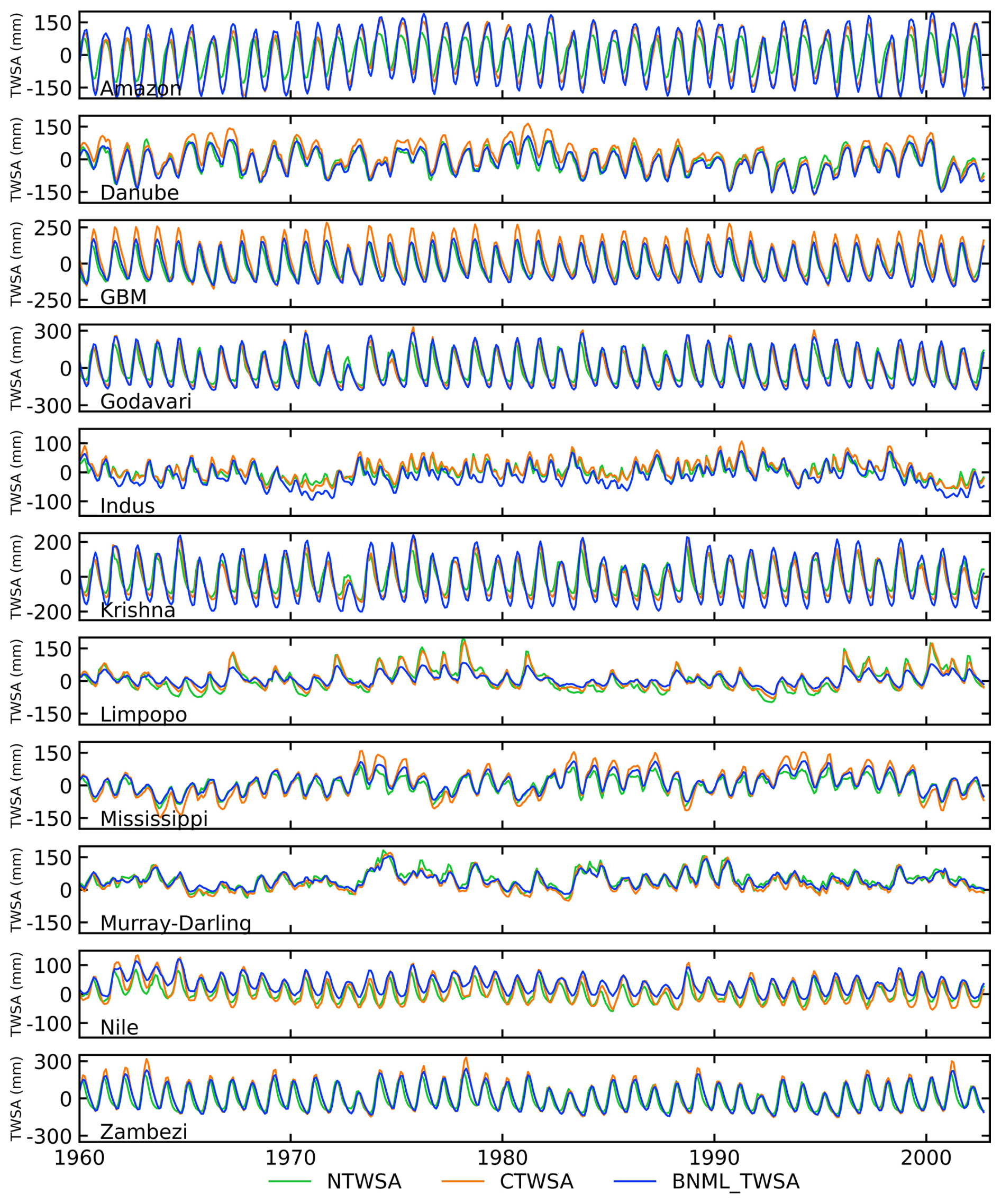
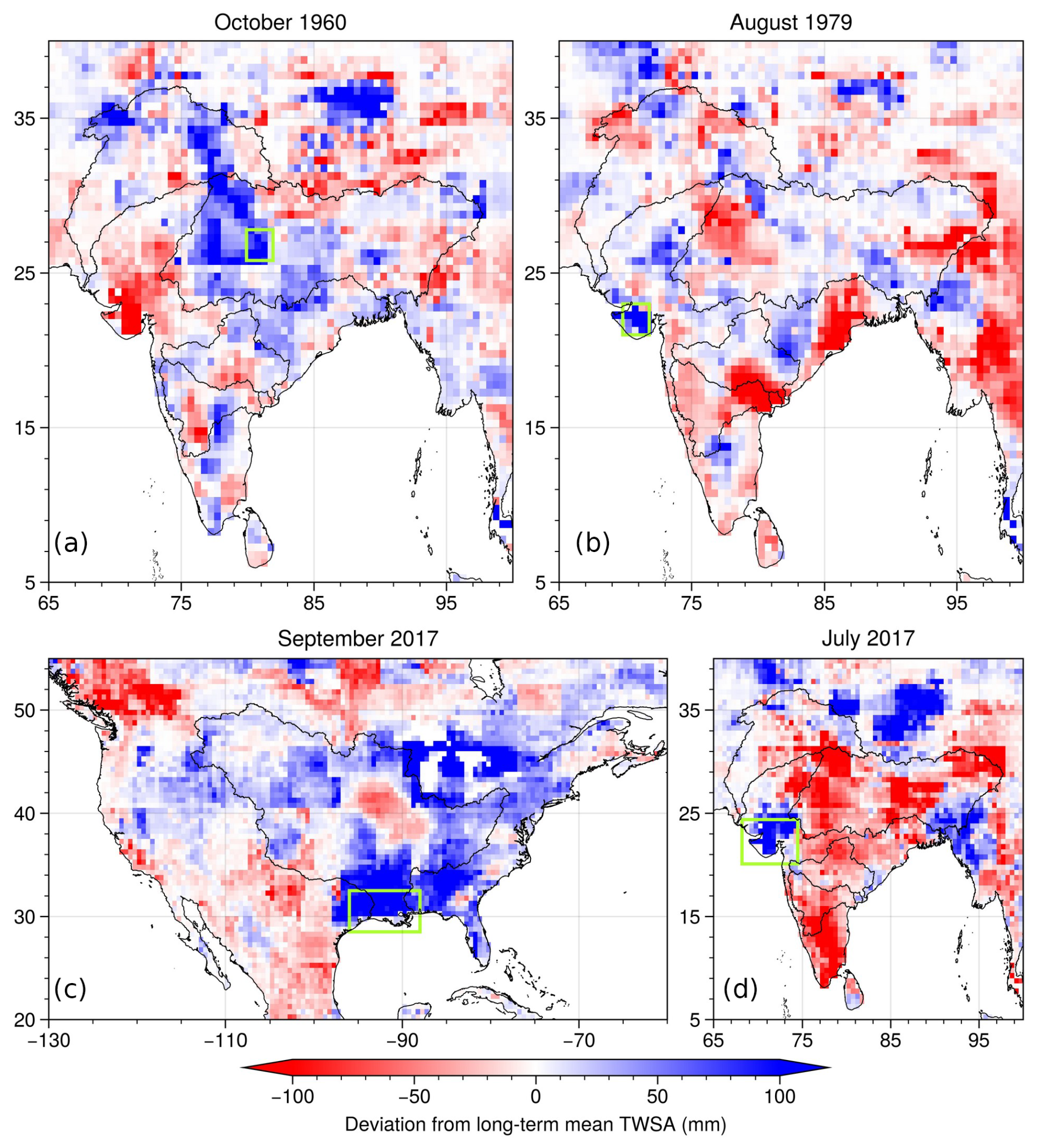
Figure 12 Difference between monthly and long-term mean monthly BNML_TWSA reflecting extreme hydroclimatic events. The zone of interest is marked by a green rectangle.

4.6 Comparison with previous studies

In this section, the reconstructed BNML_TWSA is compared with the global TWSA products developed recently by Humphrey and Gudmundsson (2019) and Sun et al. (2020). The reconstructed TWSA datasets developed using statistical models by Humphrey and Gudmundsson (2019) are named GRACE-REC. Two GRACE-REC datasets, which include monthly ensemble mean data from the JPL_MSWEP and JPL_ERA5 datasets, respectively, and the BNML_TWSA are each evaluated against the GRACE JPL mascon dataset. The grid intersection points and resolution (0.50° × 0.50°) of BNML_TWSA, GRACE-REC and GRACE JPL mascon are uniform, which eliminates the requirement for regridding. The period of comparison is selected as the common available dataset duration of the above three products. Specifically, the period spans from April 2002 to July 2019 for JPL_ERA5 and from April 2002 to December 2016 for JPL_MSWEP. Figure 13 depicts the spatial distribution of the CC values obtained from the two GRACE-REC datasets of Humphrey and Gudmundsson (2019) along with corresponding CC values of the BNML_TWSA, each compared with the GRACE JPL mascon datasets. Figures 14 and 15 depict the NSE and KGE values, respectively, similar to Fig. 13. Based on Figs. 14 and 13, it is evident that the performance of BNML_TWSA surpasses that of GRACE-REC TWSAs. This superior performance of BNML_TWSA is even more apparent in Fig. 15. Notably, both of the GRACE-REC products exhibited suboptimal performance in the region near the Sahara Desert and Saudi Arabia.

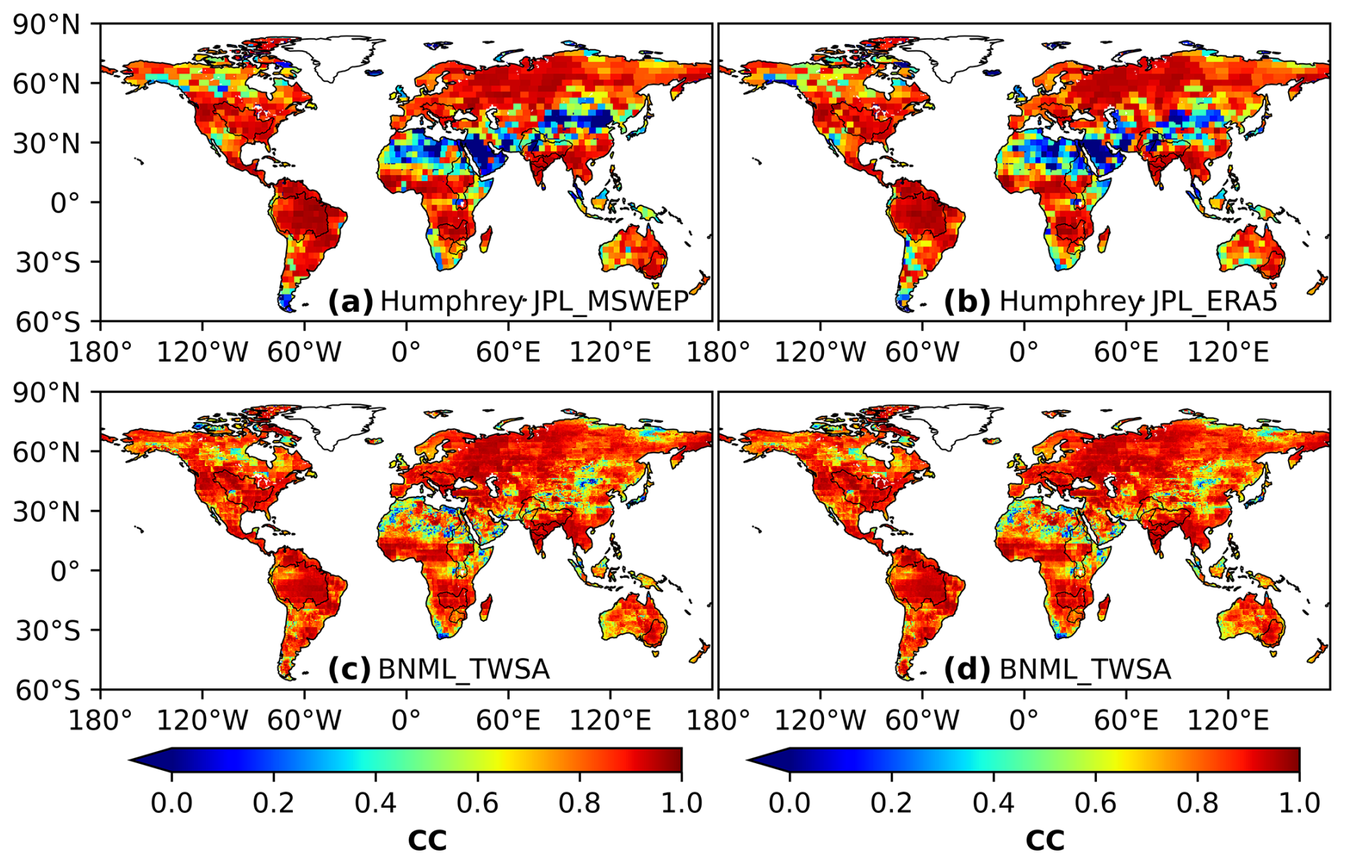
Figure 13 Comparison of correlation coefficient (CC) values obtained by two GRACE-REC products from Humphrey and Gudmundsson (2019) and BNML_TWSA, each evaluated against GRACE JPL mascon.

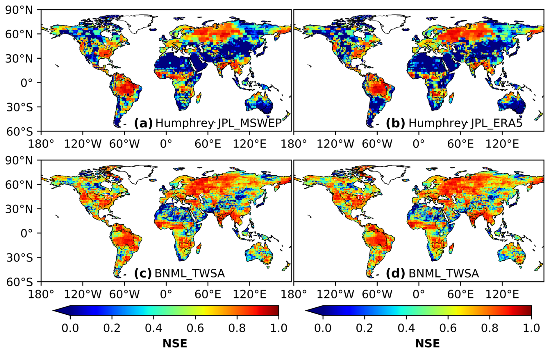
Figure 14 Comparison of Nash–Sutcliffe efficiency (NSE) values obtained by two GRACE-REC products from Humphrey and Gudmundsson (2019) and BNML_TWSA, each evaluated against GRACE JPL mascon.

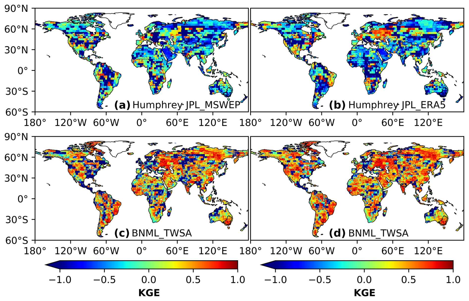
Figure 15 Comparison of Kling–Gupta efficiency (KGE) values obtained by two GRACE-REC products from Humphrey and Gudmundsson (2019) and BNML_TWSA, each evaluated against GRACE JPL mascon.

Next, we compare the agreement of BNML_TWSA with the observed GRACE JPL mascon vs. the agreement of TWSAs derived from deep neural network (DNN) models (namely, DNN_JPL-M and DNN_CSR-M for the period from April 2002 to July 2018) by Sun et al. (2020) with the same GRACE JPL mascon. During the development of the DNN_JPL-M and DNN_CSR-M TWSA products in Sun et al. (2020), the JPL mascon and CSR mascon GRACE products are respectively used as targets. These two particular products of Sun et al. (2020) are selected for comparison as the study mentions that TWSAs derived using DNN models demonstrated superior performance compared to the other two learning-based models attempted in their study. The spatial resolution of DNN_JPL-M and DNN_CSR-M is 1.0° × 1.0°, whereas the spatial resolution of BNML_TWSA and JPL mascon is 0.50° × 0.50°. To ensure a uniform spatial resolution for all TWSA products, both BNML_TWSA and JPL mascon are regridded (upscaled) to 1.0° × 1.0°, similar to DNN_JPL-M and DNN_CSR-M. Figure 16a, b and c depict the respective CC, NSE and KGE values for DNN_JPL-M, and corresponding indices for DNN_CSR-M are shown in Fig. 16d, e and f, respectively. The CC, NSE and KGE values for BNML_TWSA are depicted in Fig. 16g, h and i, respectively. The prediction accuracy of BNML_TWSA is the best when compared to DNN_JPL-M and DNN_CSR-M TWSA.

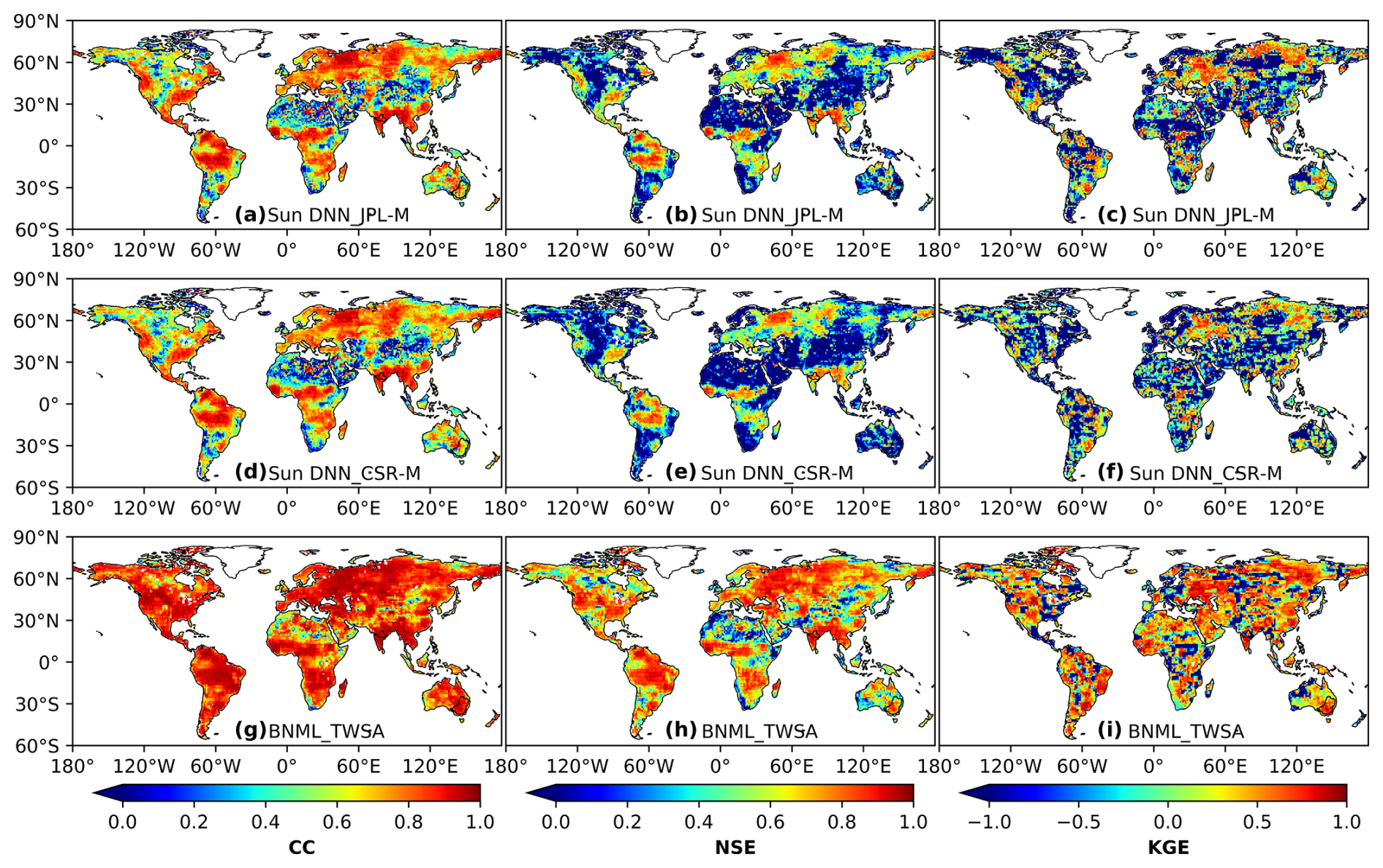
Figure 16 Comparison of correlation coefficient (CC), Nash–Sutcliffe efficiency (NSE) and Kling–Gupta efficiency (KGE) values obtained by two reconstructed TWSA products from Sun et al. (2020) and BNML_TWSA, each evaluated against GRACE JPL mascon.

The basin-wise median CC, NSE and KGE values of BNML_TWSA, the reconstructed TWSAs from Humphrey and Gudmundsson (2019), and TWSAs from Sun et al. (2020) are compared in Fig. 17 using a radar chart. Specifically, for Humphrey JPL_ERA5, the CC values are shown in Fig. 17a, the NSE values in Fig. 17d and the KGE values in Fig. 17g. Similarly, for Humphrey JPL_MSWEP, the CC values appear in Fig. 17b, the NSE values in Fig. 17e and the KGE values in Fig. 17h. The CC, NSE and KGE values of Sun DNN_JPL-M and Sun DNN_CSR-M, which have a similar analysis period, are presented in Fig. 17c, f and i, respectively. Thus, Fig.17a–c depict the basin-wise median CC values for the mentioned models, while Fig. 17d–f illustrate the basin-wise median NSE values after excluding those below 0. Similarly, Fig. 17g–i display the basin-wise median KGE values, excluding those below −1. With the exception of the Danube, GBM, Indus, and Nile river basins, the median CC values for BNML_TWSA and Humphrey JPL_ERA5 (as shown in Fig. 17a) exhibit similarity. BNML_TWSA demonstrates higher median CC values compared to Humphrey JPL_ERA5 across the aforementioned basins. Specifically, the improvements in the CC values obtained with BNML_TWSA are as follows: from 0.86 to 0.90 for the Danube, from 0.80 to 0.90 for GBM, from 0.59 to 0.77 for the Indus and from 0.70 to 0.77 for the Nile. Similarly, compared to Humphrey JPL_MSWEP (Fig. 17b), BNML_TWSA provides CC improvements, such as from 0.75 to 0.9 for the GBM region and from 0.47 to 0.74 for the Indus region. When compared with the reconstructed TWSA products by Sun et al. (2020), BNML_TWSA surpasses their accuracy, as the median CC values are high across all of the river basins (Fig. 17c). In terms of the median NSE values, BNML_TWSA outperforms Humphrey JPL_ERA5 in all of the river basins. Specifically, for BNML_TWSA, the median NSE value improves from −1.07 to 0.89 for the Murray–Darling Basin and from −0.17 to 0.77 for the Nile Basin. Similarly, BNML_TWSA exhibits improved performance compared to Humphrey JPL_MSWEP across all of the basins, particularly for the Murray–Darling Basin, where the median NSE improves from −0.24 to 0.72. While Sun DNN_JPL-M performs better than Sun DNN_CSR-M, BNML_TWSA consistently outperforms both of the aforementioned products of Sun et al. (2020) across all of the river basins. Notably, for the Nile Basin, the median NSE value improves from 0 to 0.53 with BNML_TWSA compared to Sun DNN_JPL-M. In terms of the median KGE values, BNML_TWSA also outperforms Humphrey JPL_ERA5 in all of the river basins. Similarly, except for the Limpopo and Indus basins, BNML_TWSA exhibits superior performance compared to Humphrey JPL_MSWEP in all other basins. Although Sun DNN_JPL-M performs better than Sun DNN_CSR-M, BNML_TWSA consistently outperforms both products, except in the Danube Basin, where Sun DNN_JPL-M has a marginally higher KGE value than BNML_TWSA.

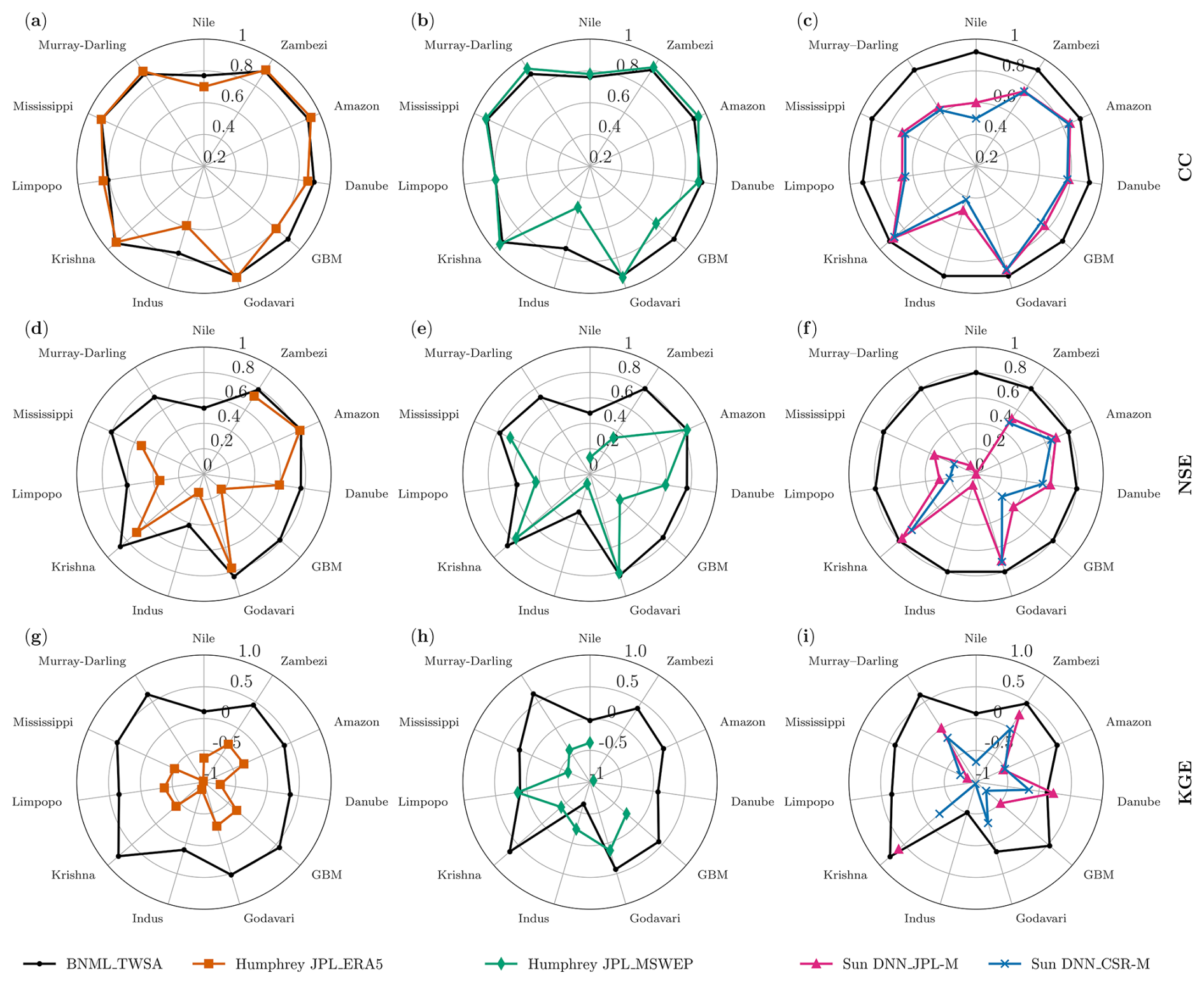
Figure 17 Comparison of the median values of the correlation coefficient (CC), Nash–Sutcliffe efficiency (NSE) and Kling–Gupta efficiency (KGE) across different basins. Note that median NSE values below 0 and KGE values below −1 are omitted during plotting.

4.7 Comparison with streamflow measurements based on the basin-scale water balance

TWS change can be used to estimate streamflow measurement based on the water balance equation for moderately large (> 100 000 km²) river basins (Humphrey and Gudmundsson, 2019). The streamflow (Q) based on the water balance model over a watershed may be expressed as follows:

$$\begin{array}{}\text{(8)}& Q=P-\mathrm{ET}-\mathrm{\Delta }S,\end{array}$$

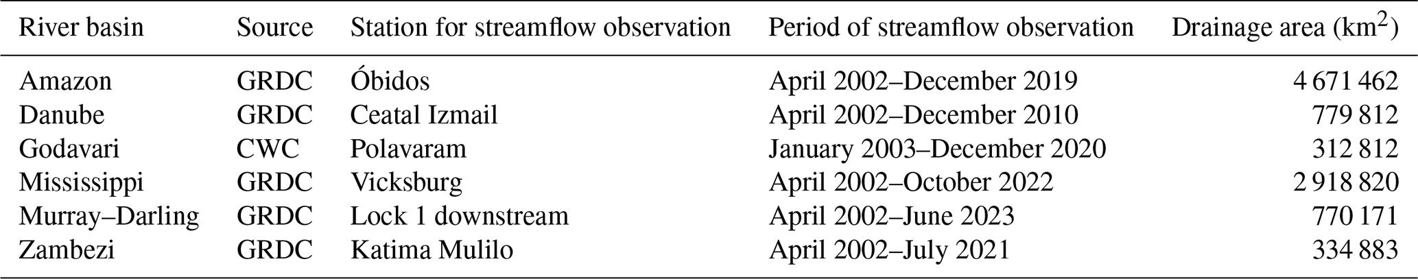
where the water balance components P and ET are precipitation and evapotranspiration, respectively, and ΔS denotes the TWS change over a time step. Comparison of evaluated streamflow using BNML_TWSA, GRACE TWSA, TWSA from Humphrey and Gudmundsson (2019) (JPL_MSWEP and JPL_ERA5), and Sun et al. (2020) (DNN_JPL-M and DNN_CSR-M) is discussed in this section. Out of the 11 river basins considered in this study, 6 basins – 1 from each continent – were selected based on the availability of streamflow data. More details on the six selected basins and their streamflow observation stations are given in Table 3. Streamflow observations are predominantly acquired from the Global Runoff Data Centre (GRDC), except for the Godavari River in India, for which the streamflow data are sourced from the Central Water Commission (CWC).

Table 3 Details of basin and streamflow observation locations for six global river basins. Data were sourced from the Global Runoff Data Centre (GRDC; https://portal.grdc.bafg.de, last access: 12 November 2024) and Central Water Commission (CWC; https://indiawris.gov.in, last access: 7 November 2023), India.

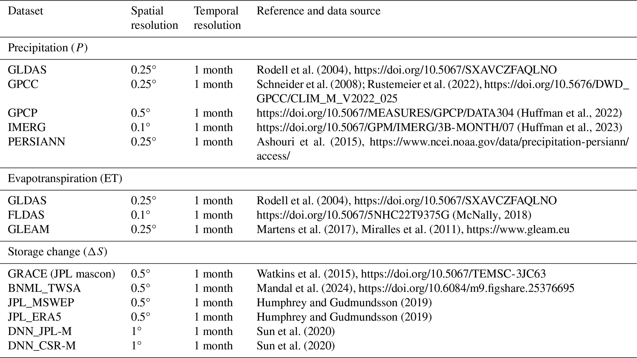
Observations of terrestrial water balance components for large river basins worldwide are limited, with sparsely distributed gauges for precipitation and even fewer observations for evapotranspiration. However, due to the availability of data from satellite sensors and outputs from global land surface models, it is possible to analyze the water balance of river basins with sparse observations. Details of the collected dataset and sources are presented in Table 4. Precipitation (P) data from five different sources were collected for each grid cell within these river basins. The basin-scale average of all five precipitation products (GLDAS, GPCC, GPCP, IMERG and PERSIANN) is considered to be the “observed” precipitation for that particular basin. Similarly, for evapotranspiration (ET), the average of three products (GLDAS, FLDAS and GLEAM) is considered the observed ET for that basin. In this study, ΔS for the tth month is calculated as the central difference in the TWSAs, as shown below.

$$\begin{array}{}\text{(9)}& \mathrm{\Delta }S={\displaystyle \frac{({\mathrm{TWSA}}_{t+\mathrm{1}}-{\mathrm{TWSA}}_{t-\mathrm{1}})}{\mathrm{2}}}\end{array}$$

Rodell et al. (2004)Schneider et al. (2008); Rustemeier et al. (2022)(Huffman et al., 2022)(Huffman et al., 2023)Ashouri et al. (2015)Rodell et al. (2004)(McNally, 2018)Martens et al. (2017)Miralles et al. (2011)Watkins et al. (2015)Mandal et al. (2024)Humphrey and Gudmundsson (2019)Humphrey and Gudmundsson (2019)Sun et al. (2020)Sun et al. (2020)

Table 4 Overview of global precipitation, evapotranspiration and storage change data products utilized for streamflow calculations.

Using the water balance components described in the previous section, the streamflow for each basin is calculated using various TWSA products, including GRACE, BNML_TWSA, JPL_MSWEP, JPL_ERA5, DNN_JPL-M and DNN_CSR-M. This computation is performed based on the terrestrial water balance equation (Eq. 8). The computed Q values are compared with the observed Q values from the station, and the corresponding correlation coefficients (CC) are determined. Figure 18 presents the correlation coefficient (CC) values as a heatmap for all six river basins, highlighting the performance of BNML_TWSA. For the Amazon Basin, BNML_TWSA demonstrates strong performance, with a CC of 0.89, comparable to GRACE and JPL_MSWEP (CC: 0.9) and JPL_ERA5 (CC: 0.89). In the Danube and Godavari basins, BNML_TWSA outperforms all other TWSA products, achieving the highest CC values, although other products also perform well. For the Mississippi Basin, BNML_TWSA, along with DNN_JPL-M and DNN_CSR-M, achieves the highest CC value of 0.7. For the Murray–Darling Basin, all TWSA products show minimal CC values due to the negligible magnitude of observed streamflow at the basin outlet. For the Zambezi Basin, JPL_MSWEP performs best, with a CC of 0.46, whereas BNML_TWSA achieves a CC value of 0.35. This evaluation highlights the superior and/or comparable performance of BNML_TWSA across most basins. The time series of the streamflow computed using BNML_TWSA (Q_{BNML_TWSA}) is presented alongside the observed streamflow (Q_Observed) and the streamflow computed using GRACE TWSA (Q_GRACE) in the left columns of Fig. 19. The time-series plot (Fig. 19) clearly demonstrates that Q_{BNML_TWSA} aligns more closely with Q_Observed compared to Q_GRACE. Additionally, the RMSE has been computed for Q_GRACE and Q_{BNML_TWSA} against Q_Observed. These RMSE values clearly indicate the superior performance of Q_{BNML_TWSA} for all six basins compared to Q_GRACE. For the Murray–Darling Basin, the magnitude of Q_Observed is negligible due to the large amount of water withdrawal for irrigation and consumption, in addition to heavy regulation (Candogan Yossef et al., 2012). All TWSA products struggle to capture the pattern of low streamflow in the Murray–Darling Basin.

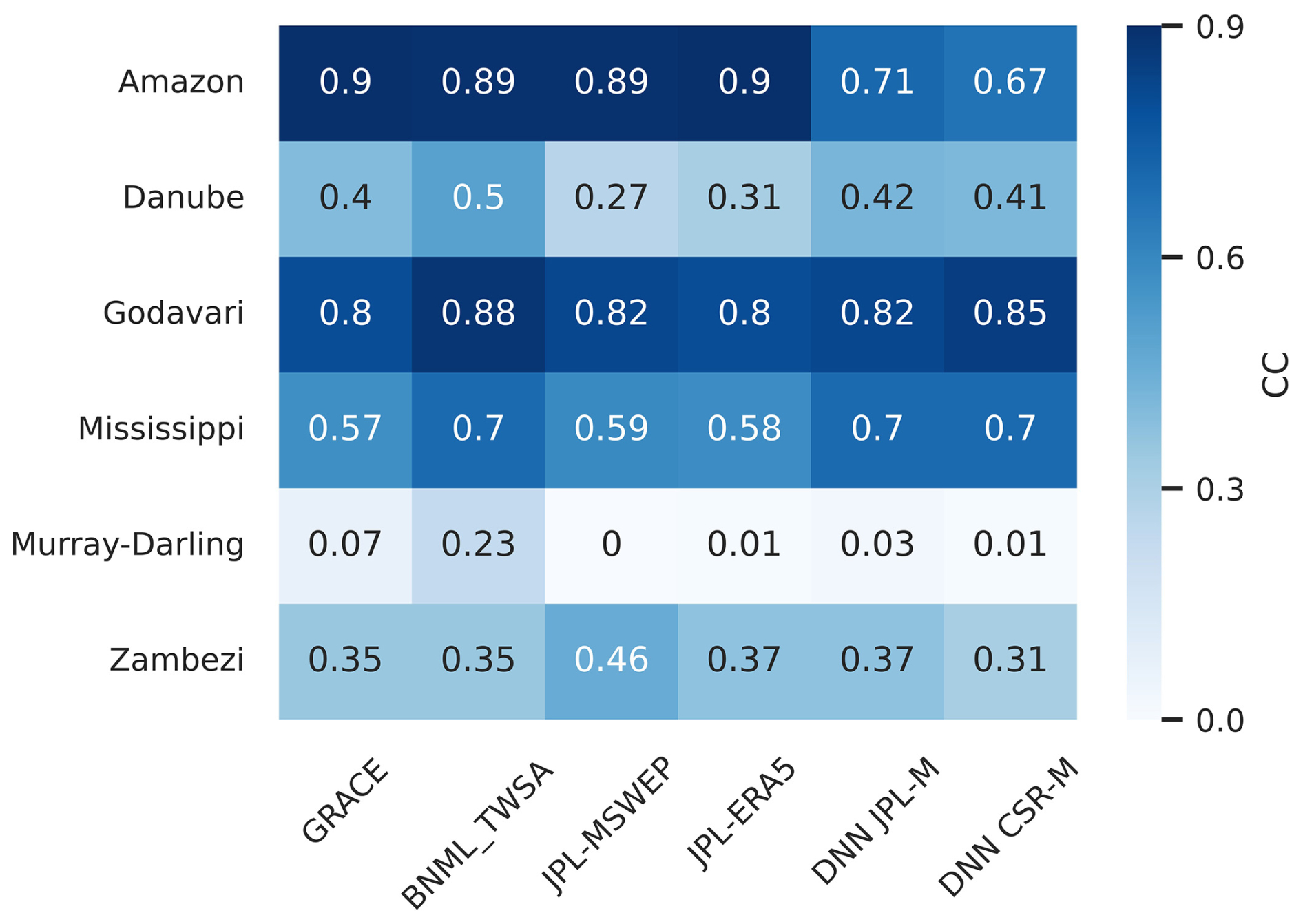
Figure 18 Basin-wise CC values obtained against observed Q and computed Q from water balance using TWSA data from GRACE, BNML_TWSA and other studies.

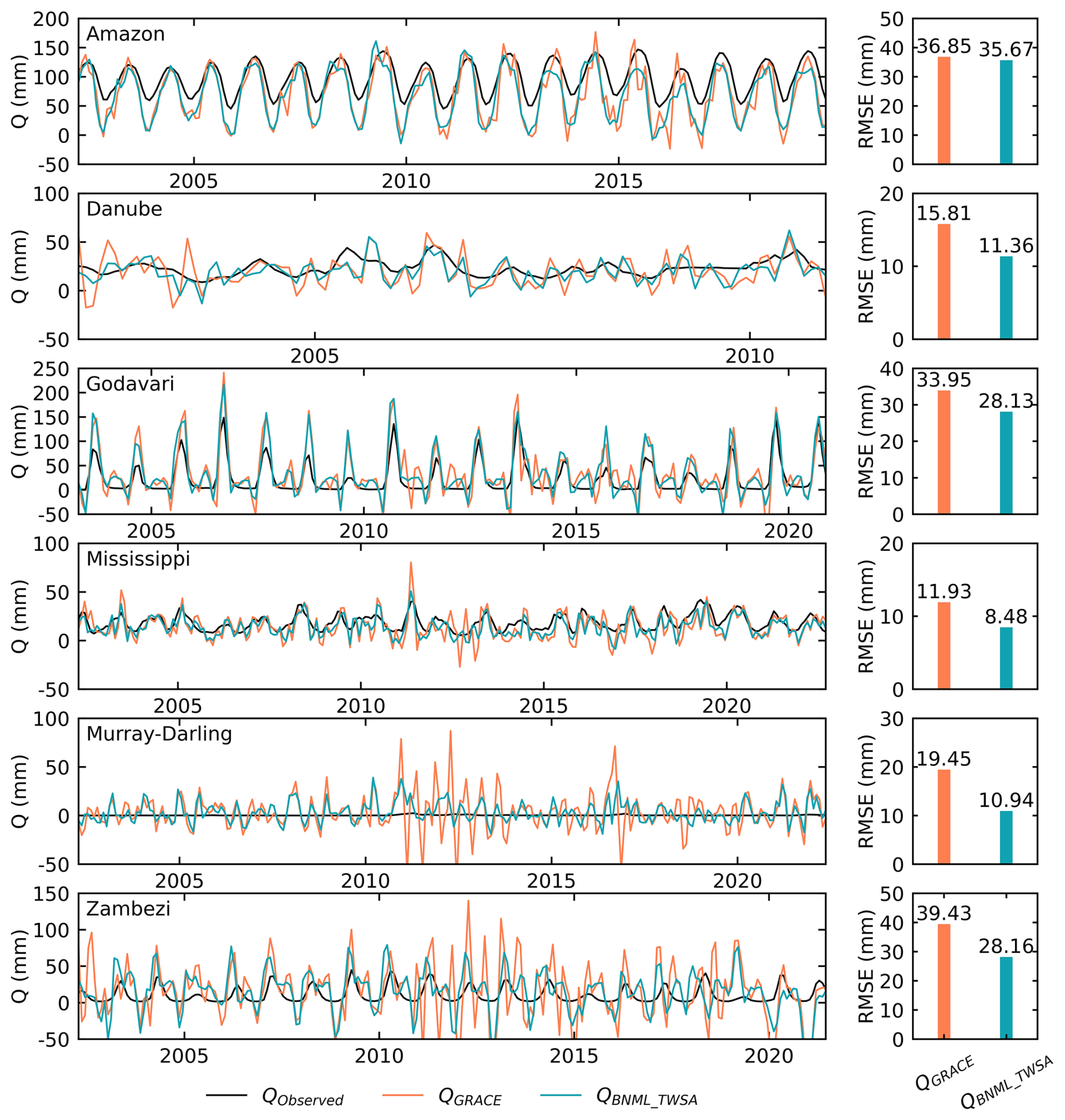
Figure 19 Comparison of observed streamflow (Q_Observed), Q obtained from water balance using GRACE TWS data (Q_GRACE) and Q obtained from water balance using BNML_TWSA TWS data (Q_{BNML_TWSA}). RMSE values (right columns) obtained for Q_GRACE and Q_{BNML_TWSA} against Q_Observed.

4.8 Uncertainty, limitations and future scope

There are various sources that contribute to the uncertainties in reconstructed TWSAs. The primary source of uncertainties arises from the measurement errors, inherent processing errors, leakage errors and model assumptions associated with the original GRACE data, as documented by Boergens et al. (2022) and Gao et al. (2023). Nevertheless, this issue is effectively mitigated by utilizing the mascon solution, which demonstrates clear superiority over the spherical harmonics data (Kalu et al., 2024). The JPL mascon solution employs a coastline resolution improvement (CRI) filter to minimize leakage errors across land–ocean boundaries. Additionally, gain factors are utilized to further mitigate these leakage errors. Moreover, a Bayesian framework is implemented to more effectively eliminate correlated errors compared to traditional empirical filters (Wiese et al., 2016). Another source of uncertainty stems from the ML models, which may be categorized into contributions from inadequacies and/or lack of knowledge regarding the model (epistemic) and data noise (aleatoric). In the present study, epistemic uncertainty has been reduced to some extent by training four different ML models at each grid cell and selecting the best-performing model to reconstruct the BNML_TWSA globally. On the other hand, aleatoric uncertainty may arise from the input dataset (i.e., the selected predictors). Analyzing the spatial distribution of selected predictors using BNs (Fig. 2), it becomes apparent that commonly employed forcing variables, such as precipitation (P) and temperature (T), do not rank among the top predictors in most grid cells. This observation suggests that these forcing variables are already accounted for in the LSMs, as indicated by Sun et al. (2019). However, these variables are still selected as optimal predictors in some of the grid cells, which implies that physics-based LSMs may not entirely capture the total information encapsulated in the raw data. Consequently, incorporating a diverse set of variables – including those already utilized in physics-based LSMs – as potential predictors could mitigate model structural errors and parameter uncertainties inherent in the LSMs (Sun et al., 2020, 2019). Furthermore, uncertainties may also depend on the actual source of the input variables. For example, precipitation from satellite sources will entail different uncertainties compared to LSM-based precipitation. In the present study, aleatoric uncertainty may arise from the absence of variables that capture the impact of anthropogenic activities. As we utilized variables from LSMs and climate indices as inputs to the ML models for reconstructing BNML_TWSA, the influence of anthropogenic activities is not adequately represented by these variables.

In this study, a model uncertainty assessment is performed for the reconstructed dataset during the model training phase, using the GRACE observations. The uncertainty in the model predictions is quantified by calculating confidence intervals (CIs) of the TWSA estimates. The CI is defined as the point estimate ± the margin of error, where the margin of error is determined by the product of a confidence coefficient (C_confidence), derived from the standard normal curve, and the standard error in the point estimate. The standard error in the point estimate is computed using the residuals from the training set employed in the ML model. The residuals (ε) are calculated as the difference between GRACE JPL mascon and the reconstructed BNML_TWSA during the training period, as outlined below:

$$\begin{array}{}\text{(10)}& {\mathrm{GRACE}}_t=\mathrm{BNML}\mathrm{\_}{\mathrm{TWSA}}_t+\mathit{\epsilon }.\end{array}$$

These residuals capture errors arising from data noise and structural model inaccuracies, as discussed earlier. A classical approach to determining the standard error (σ_ε) of the residuals is given by the following:

$$\begin{array}{}\text{(11)}& {\mathit{\sigma }}_{\mathit{\epsilon }}=\sqrt{\mathrm{variance}\left(\mathit{\epsilon }\right)}.\end{array}$$

For most grid cells, the residuals follow a normal distribution (Fig. 20a). The normality of the residuals was verified using the Shapiro–Wilk test, with normality assumed when the p value exceeds 0.05. Consequently, it is appropriate to use the standard error to estimate the confidence interval (Humphrey and Gudmundsson, 2019). The confidence interval is calculated as follows:

$$\begin{array}{}\text{(12)}& \mathrm{95}\mathit{\%}\mathrm{CI}=\text{Point estimate}\pm C_{\mathrm{confidence}}\times {\mathit{\sigma }}_{\mathit{\epsilon }}.\end{array}$$

The spatial distribution of the standard error (σ_ε) is shown in Fig. 20b. The σ_ε values for grid cells in arid regions are significantly smaller compared to those in other regions, indicating improved accuracy in arid areas. This observation aligns with the findings of Humphrey and Gudmundsson (2019).

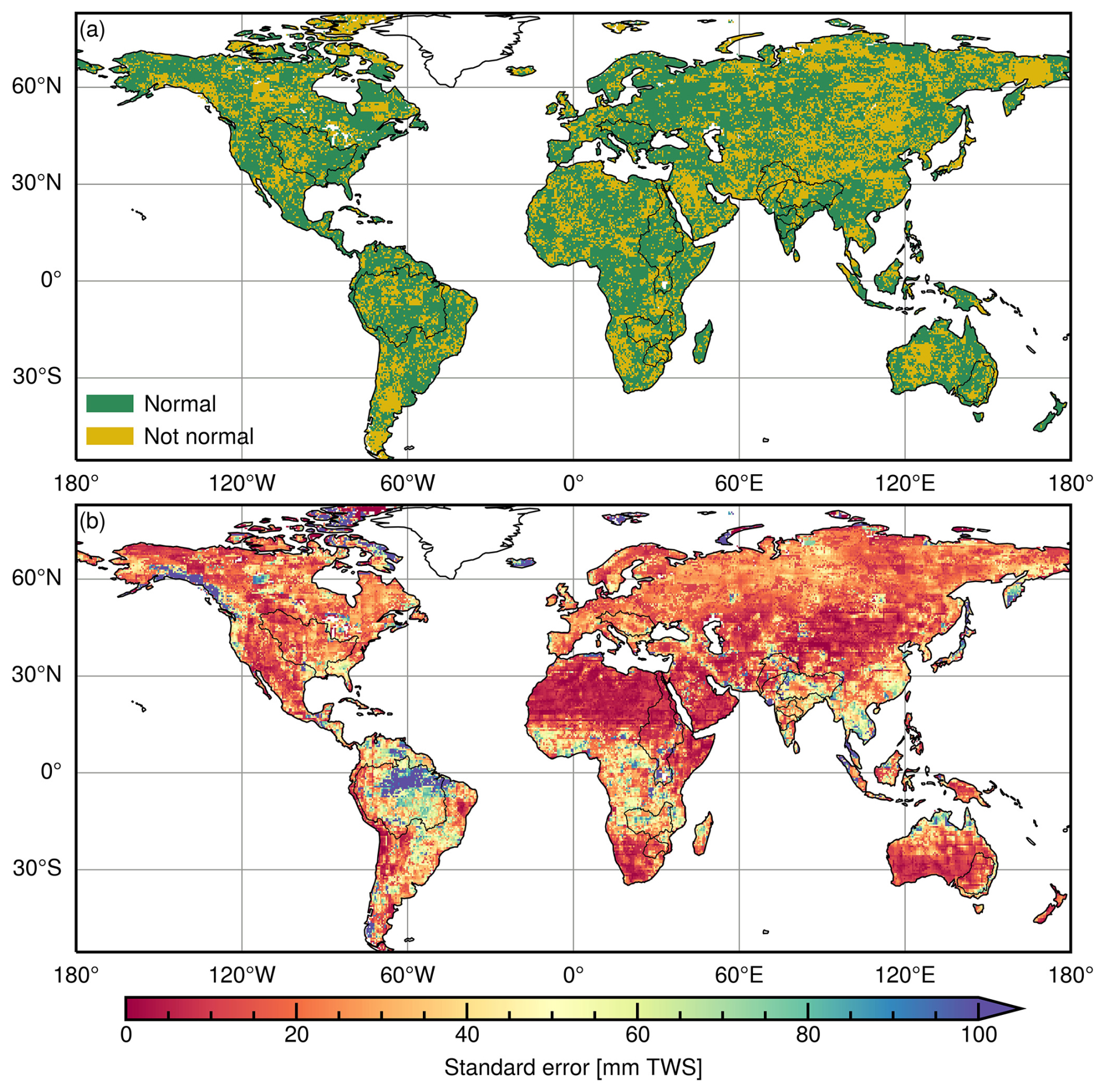
Figure 20 Characteristics of residuals of reconstructed BNML_TWSA computed against GRACE JPL mascon during the training period: (a) the Shapiro–Wilk normality test result on residuals; (b) the standard error of the residuals.

Climate change and anthropogenic activities are critical factors that can introduce additional uncertainties into the assessment of TWS. These uncertainties arise from factors such as land-use changes, irrigation practices and urbanization, which significantly influence regional water storage dynamics. In this study, variables derived from LSMs were utilized as potential predictors. However, future research could benefit from incorporating input variables from GHMs to better account for anthropogenic influences. GHMs are particularly well suited for modeling human interventions in water resources, offering a more realistic representation of these activities (Bibi et al., 2024). It is important to acknowledge that both LSMs and GHMs have inherent limitations when utilized as physically based sources of TWSAs (Bibi et al., 2024). The integration of ML models with physical models can help address these limitations, reducing errors in hydrological analyses (Xu et al., 2014). Numerous studies have demonstrated that ML models frequently outperform traditional hydrological models in various applications (Kim and Kim, 2021; Liang et al., 2023). This suggests that leveraging ML models, alongside advancements in physical modeling, holds great promise for improving the accuracy and reliability of hydrological assessments.

5 Data availability

The presented dataset is published at https://doi.org/10.6084/m9.figshare.25376695 (Mandal et al., 2024), and updates will be published as and when needed. The BNML_TWSA dataset is available for all grid cells globally, with a spatial resolution of 0.50° × 0.50°, similar to the GRACE JPL mascon, and is provided in NetCDF format. The inputs to the ML models and the optimal predictors selected using BNs at each grid cell globally are also published. Additionally, the uncertainty associated with the BNML_TWSA is made available in terms of standard error, provided as a NetCDF file. All datasets utilized in this study are readily accessible; comprehensive dataset information, along with the respective links, is provided in this section. JPL GRACE mascon data are obtained from the Physical Oceanography Distributed Active Archive Center (NASA/JPL, 2023, https://doi.org/10.5067/TEMSC-3JC63; Watkins et al., 2015, https://podaac.jpl.nasa.gov/dataset/TELLUS_GRAC-GRFO_MASCON_CRI_GRID_RL06.1_V3). TWS data are retrieved from NASA GLDAS CLSM simulations (Li et al., 2019) (https://doi.org/10.5067/LYHA9088MFWQ, Li et al., 2018; https://doi.org/10.5067/TXBMLX370XX8, Li et al., 2020). Canopy surface water, soil moisture content, snow water, precipitation and temperature data are taken from the GLDAS Noah Land Surface Model (Rodell et al., 2004) (https://doi.org/10.5067/9SQ1B3ZXP2C5, Beaudoing and Rodell, 2019; https://doi.org/10.5067/SXAVCZFAQLNO, Beaudoing and Rodell, 2020). The Dipole Mode Index is taken from the National Oceanic and Atmospheric Administration (NOAA) Physical Sciences Laboratory (Saji et al., 1999; Saji and Yamagata, 2003) (https://psl.noaa.gov/gcos_wgsp/Timeseries/Data/dmi.had.long.data). North Atlantic Oscillation data (Wallace and Gutzler, 1981; Barnston and Livezey, 1987) (https://www.cpc.ncep.noaa.gov/products/precip/CWlink/pna/norm.nao.monthly.b5001.current.ascii) and the Oceanic Niño Index (Bamston et al., 1997) (https://www.cpc.ncep.noaa.gov/data/indices/oni.ascii.txt) are retrieved from the NOAA Climate Prediction Center.

6 Code availability

We have used standard Python packages such as tensorflow, keras, sklearn and mlxtend to build the ML models, while matplotlib was employed to generate the plots. No specific software tools for ML were used. For reproducibility, the Python codes used to build the ML models are available from the same DOI-based repository: https://doi.org/10.6084/m9.figshare.25376695 (Mandal et al., 2024).

7 Conclusions

In this study, we utilized Bayesian networks (BNs), a novel predictor selection technique, and machine learning (ML) models to reconstruct the global terrestrial water storage anomaly (BNML_TWSA) product, which is a GRACE-like TWSA dataset, thereby filling data gaps in GRACE and generating hindcasts for the pre-GRACE period. The major conclusions from this study are outlined below.

For the target TWSAs, optimal inputs are selected among meaningful predictor variables, such as land surface model outputs (TWSA from the Catchment Land Surface Model, CTWSA, and the Noah Land Surface Model, NTWSA), meteorological variables (precipitation and temperature) and climate indices (the Dipole Mode Index, DMI; the North Atlantic Oscillation, NAO; and the Oceanic Niño Index, ONI). It is observed that the climate indices, ONI and DMI, are selected by BNs as optimal predictors for a large number of grid cells globally, along with TWSAs from LSM outputs. This establishes that, in addition to the available LSM-based TWSA products, large-scale climate indices are more important predictors of TWSAs than the local meteorological inputs.

At the global scale, convolutional neural network (CNN), support vector regression (SVR), extra trees regressor (ETR) and stacking ensemble regression (SER) models are employed following the selection of optimal predictors through BNs at each grid cell to finally obtain BNML_TWSA. It is noted that a single ML model cannot perform optimally across all grid cells worldwide, due to the significant spatial variability in the important predictors. However, the performance of ETR is found to be the best for most of the grid cells within the Ganga–Brahmaputra–Meghna, Godavari, Krishna, Limpopo and Nile river basins. ETR performs best in 44 % grid cells worldwide followed by SVR, SER and CNN.

The proposed approach yields a more reliable estimate of TWS compared to the outputs of global hydrological models (GHMs) and land surface models (LSMs), which have significant biases due to inherent uncertainty and a lack of representation of some of the physical processes. BNML_TWSA outperforms NTWSA and CTWSA for most grid cells worldwide. For river basins such as the Indus and Nile, BNML_TWSA matches GRACE TWSAs very closely, even during the period when the TWSAs from LSM outputs deviate substantially from GRACE TWSAs. With respect to evaluating the basin-wise average BNML_TWSA against GRACE TWSAs, the Zambezi Basin in Africa exhibited the highest correlation coefficient (CC = 0.989), followed by the Godavari (CC = 0.984) and Krishna (CC = 0.983) basins in India. Further, the accurate reflection of historical extreme climate events, such as major floods, via the hindcasted BNML_TWSA supports the enhanced accuracy of the proposed model and the developed TWSA dataset. A comparative analysis with TWSA products developed in recent literature (Humphrey and Gudmundsson, 2019; Sun et al., 2020) indicates that BNML_TWSA surpasses these datasets when evaluated against the overlapping GRACE period. Additionally, streamflow, computed as residuals of the water balance derived using BNML_TWSA and the TWSAs developed in recent literature, has been evaluated against observed streamflow across six global river basins. The evaluation revealed a reasonably good correlation for BNML_TWSA. Furthermore, the uncertainty associated with BNML_TWSA is assessed for each grid cell in the form of standard error (σ_ε). The results showed that the standard error of the BNML_TWSA exhibits a smaller magnitude in grid cells located in arid regions compared to those in other regions. Hence, this study demonstrates that the proposed BN- and ML-based approach can effectively learn complex relationships between various inputs and GRACE TWSAs, enabling global reconstruction and hindcasting of TWSAs, which is essential for several hydroclimatological studies.