An expert survey on chamber measurement techniques and data handling procedures for methane fluxes

Methane is an important greenhouse gas, but the magnitude of global emissions from natural sources remains highly uncertain. To estimate methane emissions on large spatial scales, methane flux data sets from field measurements collected and processed by many different researchers must be combined. One common method for obtaining in situ methane flux measurements is flux chambers. We hypothesize that considerable uncertainty might be introduced into data synthesis products derived from chamber measurements due to the variety of measurement setups and data processing and quality control approaches used within the chamber flux community. Existing guidelines on chamber measurements promote more standardized measurement and data processing techniques, but, to our knowledge, so far, no study has investigated which methods are actually used within the chamber flux community. Therefore, we aimed to identify the key discrepancies between the measurement and data handling procedures implemented for chamber methane fluxes by different researchers.

We conducted an expert survey to collect information on why, where, and how scientists conduct chamber-based methane flux measurements and how they handle the resulting data. We received 36 responses from researchers in North America, Europe, and Asia, which revealed that 80 % of respondents have adopted multi-gas analyzers to obtain high-frequency (< 1 Hz) methane concentration measurements over a total chamber closure time of, typically, between 2 and 5 min. Most but not all of the respondents use recommended chamber designs, including features such as airtight sealing, fans, and a pressure vent. We presented a standardized set of methane concentration time series recorded during chamber measurements and derived CH₄ flux estimates based on the processing and quality control approaches suggested by the survey participants. The responses showed broad disagreement among the experts concerning the processes that they consider to be responsible for non-linear methane concentration increases. Furthermore, there was a tendency to discard low or negative CH₄ fluxes. Based on the expert responses, we estimated a variability of 28 %, introduced by different researchers deciding differently on discarding vs. accepting a measurement when processing a representative data set of chamber measurements. Different researchers choosing different time periods within the same measurement for flux calculation caused an additional variability of 17 %. Our study highlights the importance of understanding the processes causing the patterns in CH₄ concentrations visible from high-resolution analyzers, as well as the need for standardized data handling procedures in future chamber methane flux measurements. This is highly important to reliably quantify methane fluxes all over the world.

The survey results, as well as the questionnaire, are publicly available at https://doi.org/10.1594/PANGAEA.971695 (Jentzsch et al., 2024b).

1 Introduction

Methane (CH₄) is an important greenhouse gas with 45 times the global warming potential of carbon dioxide (CO₂) on a 100-year timescale (Neubauer, 2021). However, emission estimates differ largely between “top-down” atmospheric measurement inversions and “bottom-up” approaches using data-constrained or process-based models (Kirschke et al., 2013; Saunois et al., 2020). Natural emissions, especially bottom-up estimates of wetland emissions, are the largest source of uncertainty with regard to the global CH₄ budget due to the poorly constrained areal extent of wetlands and other methane-producing ecosystems like lakes, streams, and reservoirs; highly uncertain CH₄ process parameterization; and a lack of validation data sets (Melton et al., 2013; Saunois et al., 2020).

One approach to obtain large-scale validation data sets for CH₄ fluxes has been to create synthesis data sets of measurements collected by multiple researchers using chamber-based methane flux measurements (Kuhn et al., 2021; Treat et al., 2018). An advantage of using the closed-chamber technique over in situ measurements operating on larger spatial scales is that the resulting data sets can capture the high spatial and temporal variability in natural CH₄ emissions with small-scale spatial changes in environmental and ecological conditions (Frenzel and Karofeld, 2000; Laine et al., 2007; Moore and Knowles, 1990; Waddington and Roulet, 1996). When applying the closed-chamber technique, a chamber is placed on top of the soil, and the change in gas concentrations in the chamber headspace is monitored over time to estimate the exchange of CH₄ between soil, plants, and the atmosphere on the microscale (e.g., Livingston and Hutchinson, 1995). The rate of change in gas concentrations, after correcting for temperature and pressure conditions using the ideal gas law, is then used to compute the flux of CH₄ through the surface area covered by the chamber (Holland et al., 1999). However, despite more than 30 years of chamber-based methane flux measurements from wetland ecosystems, developing large-scale methane validation data sets remains challenging.

Two approaches are typically used for measuring the CH₄ concentrations inside the chamber: manual sampling and in-line gas analyzers. Manual sampling for gas concentrations involves extracting gas samples from the chamber headspace at regular time intervals using syringes and subsequently analyzing them for CH₄ concentrations on a gas chromatograph. A linear fit is then usually applied to the CH₄ concentration measurements over time, and its slope is used as the flux estimate after correction for the pressure and temperature inside the chamber (Holland et al., 1999). Manual sampling of the chamber headspace is typically characterized by a low sampling frequency which requires a relatively long chamber closure time. Here, the consideration is to balance the time needed to obtain a detectable change in CH₄ concentrations versus shorter measurement times to reduce chamber effects (Holland et al., 1999).

With the advances in laser spectroscopy, manual sampling is increasingly being replaced by continuously circling chamber air through an in-line gas analyzer which performs high-frequency (> 1 Hz), high-accuracy, real-time measurements of the CH₄ concentration. Through their portability and with reduced measurement times, such multi-gas analyzers have opened up new possibilities, particularly for the analysis of key trace gases like CH₄ and N₂O. At the same time, the high frequency and high accuracy of the concentration measurements uncover chamber-induced artifacts and events of ebullitive CH₄ emission that are superimposed onto the signal of the natural diffusion of CH₄ between soil, plants, and the atmosphere. Leakage of gas from the chamber (Hutchinson and Livingston, 2001), a saturation effect changing the concentration gradient between soil and chamber headspace over time (Livingston and Hutchinson, 1995), and natural CH₄ ebullition (Strack et al., 2005), as well as ebullition triggered by the chamber placement, can all lead to a deviation of the concentration change from the linear increase expected for a constant diffusive flux. These observations call for a reassessment of measurement, processing, and quality control (QC) approaches to minimize the influence of chamber effects on the flux estimates.

Besides the general lack of validation data sets, existing data sets that combine flux data collected by different researchers are likely to include additional uncertainty due to the variety of measurement and data handling approaches used. Several studies have assessed the difference in flux estimates resulting from different chamber setups (Pihlatie et al., 2013; Pumpanen et al., 2004) and from different data processing approaches such as using non-linear as compared to linear fits to the gas concentration measurements over time (Forbrich et al., 2010; Healy et al., 1996; Pirk et al., 2016). Such experimental and modeling studies have contributed to several guidelines for chamber measurements that were published in an attempt to establish a more standardized protocol for flux measurements. These best-practice guidelines for chamber measurements summarize recommendations on chamber designs (e.g., Clough et al., 2020), as well as on the entire workflow from measurements to data processing and quality control (e.g., de Klein and Harvey, 2012; Fiedler et al., 2022; Maier et al., 2022). While guidelines outlining best measurement practices for chamber measurements provide a well-founded summary of the methods recommended to collect high-quality flux data, chamber-based flux data sets are often lacking in detailed metadata reporting on chamber design, flux calculation, and QC methods. This introduces substantial uncertainty into comprehensive comparisons of chamber-based data.

Given that the measures outlined in guidelines for chamber measurements have significant effects on the magnitude of the CH₄ fluxes measured, we need to know how widely implemented these recommendations are and where key differences and knowledge gaps remain. Gathering scientific and technical information from experts is necessary to move beyond established theoretical knowledge and can offer further evidence to aid in decision-making (Morgan, 2014). Several studies have recently used expert assessments to gain valuable insights into topical climate-change-related issues (Macreadie et al., 2019; Rosentreter et al., 2024; Schuur et al., 2013). In this study, we use expert judgments derived from a questionnaire to identify the methods for the chamber measurements, processing, and QC of CH₄ fluxes that are actually currently used within the flux community and to assess the resulting variability and uncertainties.

This study aims to derive starting points for improving the usability of chamber CH₄ flux data sets for large-scale synthesis studies through reducing the discrepancies between the measurement and data handling approaches used within the chamber flux community, as identified from an expert survey. Our objectives were to (1) provide an overview of the chamber designs, measurement setups and routines, flux calculation, and QC approaches that are currently used by scientists to quantify CH₄ fluxes and (2) estimate the variability that is introduced into CH₄ flux data sets by the variety of data handling approaches when a representative data set of chamber measurements is processed by different researchers. Our study raises awareness with regard to the differences in the chamber methods used within the flux community – a potentially considerable but often neglected source of error in synthesis studies that combine flux data sets collected and processed by different researchers. Through identifying major sources of uncertainty resulting from the variety of measurement, calculation, and QC approaches used within the chamber flux community, we derive starting points for eliminating such error sources and rendering individual flux data sets more comparable and combinable and, thus, better suited for larger-scale synthesis studies.

2 Methods

For this study, we evaluated an expert survey conducted in 2023 that consisted of two parts, with the first part asking questions about the professional background of the participants and the field sites, as well as the measurement, calculation, and QC approaches that they use for their own chamber measurements of CH₄ fluxes, and with the second part being an exercise on visual QC of a given set of chamber measurements.

Experts were required to have a minimum level of expertise of one field season of chamber measurements of CH₄ fluxes. They were solicited using emails and conference poster presentations through professional networks, including the Permafrost Carbon Network, the C-PEAT network, and ICOS, and through identification of experts not represented in these networks to increase the number and geographic background of the participants. Altogether, 46 experts were contacted via email. To capture the variety of chamber applications and methods used within the community, we selected the survey participants to be rather independent from each other in terms of their choice of measurement and data handling approaches.

The survey was estimated to take 40 min to complete, and the survey language was English. The survey was administered using LimeSurvey (Community Edition Version 5.6.68+240625). Survey participants were asked if they wished to be acknowledged or to remain anonymous. Survey participation was voluntary and was not compensated. The survey has been legally checked by a data protection officer to comply with the EU data protection regulation and involved a privacy policy statement – explaining the use and processing of the collected data – that needed to be approved by every survey participant prior to participation. The complete, archived questionnaire and the survey responses are provided in Jentzsch et al. (2024b).

2.1 Methods of survey part 1 – the survey participants and their chamber measurements

In the first, informative part of the survey, we gathered information on the measurement, data processing, and QC approaches that the participants use for their own chamber measurements. For this part of the survey, we chose a combination of 20 choice questions (simple and multiple selection, including 7 yes-or-no questions), all of which offered the option to elaborate upon the selection(s) in a short, free-text comment, and 19 text entry questions. For a visual overview of the variety of measurement setups used, we asked the survey participants to upload a photo of their chamber system. To assess the professional background of the group of participants, we asked about their professional status, the country of their home institute, and their educational and scientific background. For an overview of the area of application of the chamber CH₄ flux measurements, we included questions on the participants' research questions and the regions and ecosystem types they usually work in. Questions on the chamber dimensions, the chamber equipment, and the measurement instruments, as well as photos thereof, together with questions on the measurement procedure and additional variables monitored, showed us the variety of experimental designs used. Additionally, we asked the participants to describe their approaches for flux calculation, quality control, and uncertainty estimation of the flux estimates.

2.2 Methods of survey part 2 – visual quality control of a standardized data set

To more directly assess the differences in terms of the interpretation of chamber data that lead to the discrepancies in measurement setups, data processing, and QC techniques, as identified in the first part of the survey, we provided a standardized set of chamber measurements for visual QC by the survey participants and extrapolated the responses to a larger, representative data set. This second part of the survey included both qualitative and quantitative responses.

The standardized set of chamber CH₄ fluxes was composed of 12 selected chamber measurements from our field campaigns at Siikaneva bog (61°50^′ N, 24°12^′ E), southern Finland, in summer 2021 and summer and fall 2022. The measurements were done using a manual chamber with a volume of 36 L and equipped with a cooling system to keep the chamber temperature close to constant, two fans to mix the air inside the chamber, and a small opening for pressure equilibration. For the measurements, the chamber was placed on collars that were permanently installed in the ground. In 2021, the connection between chamber and collar was sealed with a rubber skirt, and, in 2022, the rim between chamber and collar was filled with water to make the connection airtight. The gas concentrations inside the chamber were recorded with an in-line gas analyzer at a frequency of 1 Hz. Besides chamber measurements showing a linear increase in CH₄ concentration over time, we included examples showing a variety of deviations from the linear increase expected for constant diffusive wetland CH₄ emissions.

For visual QC of the measurements by the survey participants, we provided the concentrations of CH₄ over time, as well as the simultaneously measured concentrations of CO₂ and H₂O in the chamber, a photo of the chamber, and a description of the measurement setup, along with, for each measurement example, information on the dominant vegetation and water table depth at the measurement plot, the date and time of the measurement, whether a transparent or opaque chamber was used, the gas analyzer model, and a photo of the measurement plot (Fig. A1a in the Appendix). We asked the participants if they would keep the respective measurement for flux calculation or if they would discard it and why they would do so (Fig. A1b). If they decided to keep the measurement, we asked them to select the part of the measurement that they would use to calculate the CH₄ flux by submitting the start and end times of this period in seconds after chamber closure.

2.3 Statistical analyses

2.3.1 Cleaning of the data set

We anonymized the survey responses by separating the demographic information, including the country of the home institute, the scientific background, the highest education level, the time since PhD completion, and the current professional role of the participants, from each other and from the rest of the survey results. We furthermore removed the question regarding specific research sites before publishing the data and replaced two of the names of specific research sites, given as part of the descriptions of the main study regions, with terms for a larger region. In one response, we removed the name of another researcher mentioned by one of the participants.

We harmonized and/or categorized certain free-text responses, including the responses on the chamber shape, the chamber area, the chamber volume, the closure time of the chamber, and the frequency of the gas concentration measurements inside the chamber. From the chamber volume and chamber area, we calculate the effective chamber height. We corrected obvious writing mistakes throughout the survey as part of the standardization. In questions on QC procedures, we standardized the information regarding the exclusion of the beginning of the measurements from flux calculation, as well as the length of the excluded time period. We also adjusted the responses to questions on whether to keep or to discard a measurement in the visual QC exercise when the free-text responses clearly revealed that the wrong box had been ticked by mistake. We set the CH₄ flux to zero in two cases where survey participants clearly stated in their free-text responses that this is how they would handle the presented measurement.

2.3.2 Evaluating the visual QC exercise

We quantitatively and qualitatively evaluated the responses to the visual QC portion of the survey. We summarized the reasons for keeping or discarding a measurement as elaborated upon in the free-text responses to the visual QC part of the survey. Then, we numerically evaluated the visual QC performed on the 12 example measurements. This allowed us to quantify the variation in fluxes due to the differences in terms of the quality control and fitting approaches among researchers. For this, we calculated the CH₄ fluxes for each researcher for each of the 12 example measurements using the time periods selected by the researcher.

To calculate the fluxes, we used a standard linear fitting approach and accounted for differences in temperature and pressure among the measurements (Holland et al., 1999). The ideal gas law was used to convert the rate of change in CH₄ concentrations ($\frac{\mathrm{d}{c}_{{\mathrm{CH}}_{\mathrm{4}}}}{\mathrm{d}t}$), in ppm s⁻¹, to the molecular CH₄ flux ($F_{{\mathrm{CH}}_{\mathrm{4}}}$), in mol m⁻² s⁻¹, for each measurement example i (i= 1,…,n, where n= 12) and each survey participant j (j= 1,…,m, where m= 36).

$$\begin{array}{}\text{(1)}& F_{{\mathrm{CH}}_{\mathrm{4}i,j}}={{\displaystyle \frac{\mathrm{d}{c}_{{\mathrm{CH}}_{\mathrm{4}}}}{\mathrm{d}t}}}_{i,j}\times {\mathrm{10}}^{-\mathrm{6}}\times {\displaystyle \frac{p}{R\times T_i}}\times {\displaystyle \frac{V_i}{A}}\end{array}$$

In the above, p represents the standard atmospheric pressure of 101 325 Pa, T (°K) is the mean temperature inside the chamber during the closure, and A is the surface area of the chamber in m². V_i is the volume of the chamber used in measurement i, calculated by $V_i=A\times h_i$, where h_i is the effective height of the chamber headspace during measurement i (in m), calculated as the mean of the height above the soil surface or vegetation cover that was measured at three points around the chamber for each measurement plot. R is the ideal gas constant of 8.314 kg m² mol⁻¹ K⁻¹ s⁻². We then converted the molecular CH₄ flux into the more commonly used mass flux of CH₄ using the molar mass of CH₄ of 16.04 g mol⁻¹. For each measurement example and each participant, $\frac{\mathrm{d}{c}_{{\mathrm{CH}}_{\mathrm{4}}}}{\mathrm{d}t}$ was estimated as the slope of a linear fit (lm function from the stats package in R version 4.3.0) to the CH₄ concentrations within the time period selected by the researcher. For reasons of consistency, we used a linear fit even in the 12 cases where a participant suggested using a non-linear fit instead (7 % of the total of 173 times where the start and end times for flux calculation were given by a participant). When a measurement was accepted by an expert but no start and end times were given for flux calculation, we estimated the flux based on the entire chamber measurement.

We used the fluxes calculated from the quantitative responses to assess the variability in CH₄ flux estimates and QC procedures due to different researchers processing the measurement data, that is (1) the variability in flux estimates introduced by different researchers selecting different time periods for flux calculation and (2) the variability in the share of measurements kept for flux calculation during QC. In a representative data set of 788 chamber measurements, collected at Siikaneva bog in 2021 and 2022 (Jentzsch et al., 2024a), we visually identified and categorized the following eight classes of measurement scenarios based on the shape of the CH₄ concentrations measured in the chamber headspace over time: linear increase, linear decrease, non-linear increase – decreasing slope, non-linear increase – increasing slope, initial jump, jump(s), inconsistent trend, and low variation. During the majority (60 %) of measurements in the Siikaneva data set, CH₄ concentrations increased linearly over time (Table A1). The second largest group, represented by 18 % of the measurements, showed a non-linear, weakening increase in CH₄ concentrations over the time of the chamber closure. During 8 % of the measurements, an abrupt jump in CH₄ concentrations in the beginning or one or several jumps at a later time during the measurements were detected. A non-linear increase in CH₄ concentrations that strengthened over time was found in 3 % of the measurements, and 2 % of the measurements had an inconsistent and abruptly changing concentration trend. Low concentration changes, showing no clear trend, and a linear decrease in CH₄ concentrations were represented by less than 1 % of the measurements. From the Siikaneva data set, we selected 12 measurement examples so that each measurement scenario was represented at least once in the visual QC exercise (Table A1).

For each measurement scenario, we estimated the variability in flux estimates introduced by different researchers choosing different time periods within the same measurement for flux calculation using the coefficient of variance (CV) across the fluxes calculated for each survey participant. To extrapolate this variability to a representative data set (the presented fluxes were chosen to capture the range of observed behavior rather than to represent the observations, as explained above), we calculated the weighted sum of the CVs based on the relative occurrence of each measurement scenario within the Siikaneva data set (Table A1). To assess the variability in QC procedures, we extrapolated the percentage of measurements kept for flux calculation to a representative data set for each participant, again using the relative occurrence of each measurement scenario within the Siikaneva data set. We then calculated the CV between the percentages of measurements kept across all survey participants.

3 Results

A total number of 36 expert researchers participated in the survey. All of them completed the survey parts on demographic information and their field sites for flux measurements. Most participants (35) answered the questions concerning their flux measurement setup, and 30 responded to the questions regarding their flux calculation and QC approaches. Participation decreased to 28 experts for the visual QC part, and an additional 2 participants dropped out after the second example measurement, resulting in a survey completion rate of 72 %.

3.1 Results of survey part 1 – the survey participants and their chamber measurements

3.1.1 Demography

The survey respondents work for universities (25 participants), research centers (11 participants), or companies (1 participant) that are located in North America, central and northern Europe, and eastern Asia (Fig. 1a). Most (89 %) of the participants have a PhD title, 41 % of whom completed their PhD within the last 7 years, 25 % of whom completed their PhD between 7 and 15 years ago, and 34 % of whom completed their PhD more than 15 years ago (Fig. 2a). Nearly all (94 %) of the participants are researchers, including two PhD students (Fig. 2b). Five individual participants specified their current roles as a Bachelor student, professor, industry leader, coordinator, and consultant, respectively. At 58 %, the majority of the survey participants have a background in geosciences, followed by biology (25 %), ecology (11 %), meteorology (8 %), environmental sciences (6 %), and physics (6 %). Three individual participants have a background in forestry, biogeosciences, and agricultural sciences, respectively. Half of the participants (52 %) are part of one or several of the following flux networks and databases: FLUXNET, ICOS, AmeriFlux, OzFlux/TERN, the European Fluxes Database Cluster, and LTER.

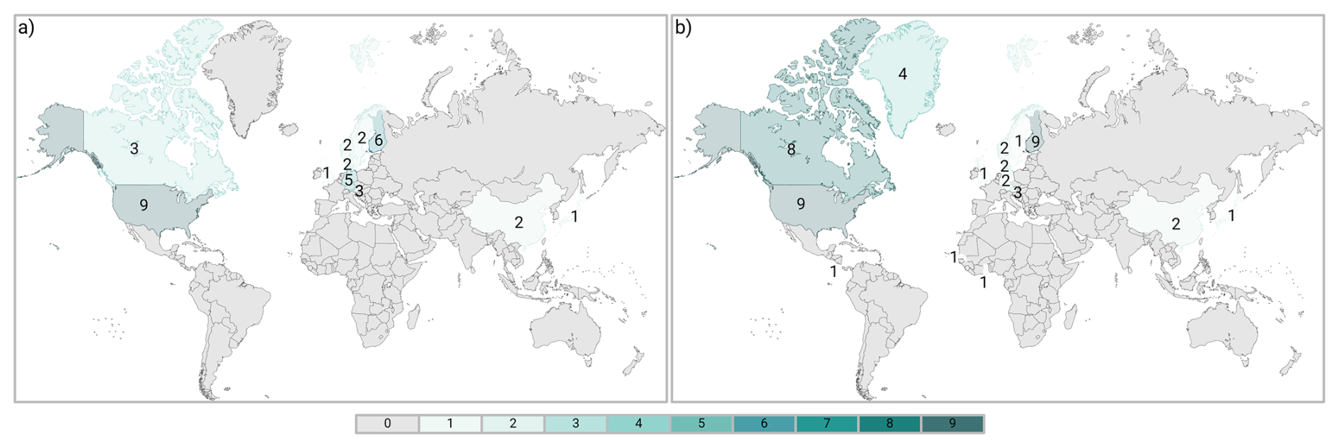
Figure 1 Countries of the main institutes (a) and of the research sites (b) of the participants. Some participants gave multiple answers regarding the country of their research sites, causing the total number of responses to exceed the total number of 36 participants. This figure was created in BioRender.

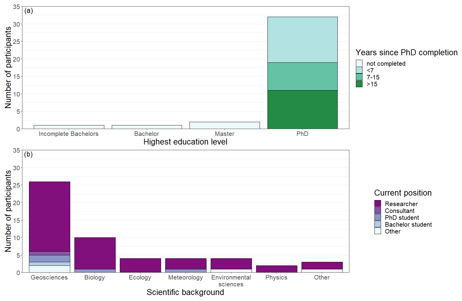
Figure 2 Histograms of the highest education level of the participants, split by the years since their PhD completion (a), and of their scientific background by current position (b). Some participants gave multiple answers regarding their scientific background, causing the total number of responses to exceed the total number of 36 participants.

3.1.2 Flux measurement sites

Most (83 %) of the participants do field measurements in the same country as their home institute, including all participants working for institutions in Asia, Canada, Finland, Norway, Denmark, Austria, and the United Kingdom (Fig. 1b). Four participants additionally reported conducting field measurements in Greenland, and three individual participants reported conducting field measurements in Ghana, Costa Rica, and Senegal, respectively, which were not among the countries of the home institutes of the participants. Six participants from the US, Germany, and Sweden have their main research sites in Canada, Finland, or Greenland according to their research questions and ecosystems of interest. The majority (83 %) of the participants focus their research on peatlands and wetlands, mainly fens or bogs (50 %) and littoral wetlands (31 %) (Fig. 3). A few (14 %) of the participants measure in (semi-)arid regions and upland areas and at sites with mineral soil instead of or in addition to wetlands. Some (33 %) of the participants explicitly mentioned field measurements in permafrost-affected landscapes; similarly, 33 % of the participants explicitly mentioned that they measure in “northern”, “boreal”, “arctic”, or “subarctic” regions, and 6 % measure in “alpine” or “subalpine” terrain. Some (25 %) of the participants do aquatic measurements, and 19 % measure at anthropogenically managed sites, such as on agricultural land and in drained and/or rewetted peatlands. Specific ecosystems researched by two participants are rice paddies and reed ecosystems.

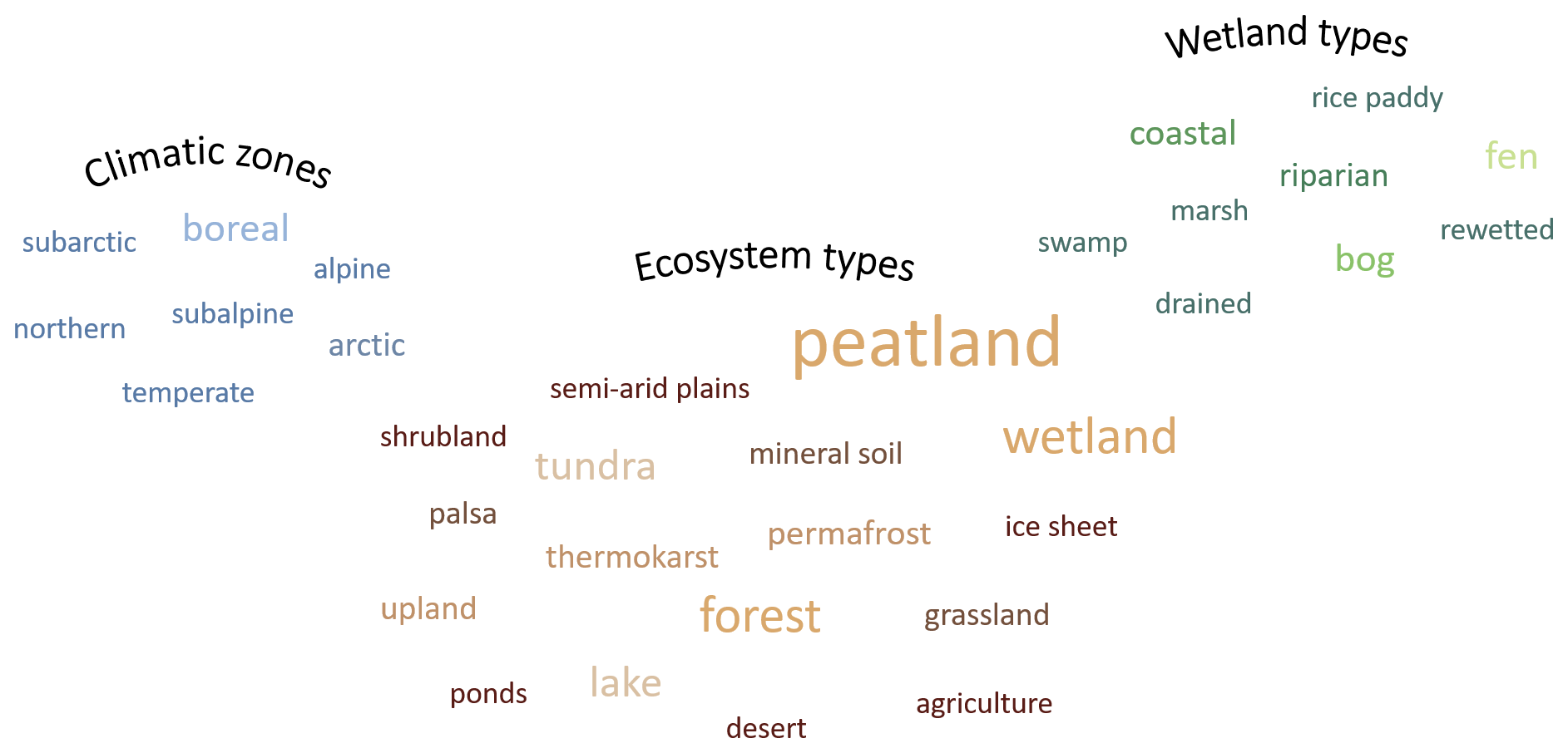
Figure 3 Word clouds of the study areas, representing the climatic zones of the study sites and the studied ecosystem types and specifying the types of wetlands and peatlands that are researched by the participants.

3.1.3 Research goals

The overarching research goals that the survey participants address with their flux measurements are to better understand the processes involved in greenhouse gas cycling, to better understand and quantify the effect of changes on greenhouse gas dynamics, to estimate greenhouse gas budgets, and to research the methodology for gas flux measurements. To investigate the environmental and ecological controls on the greenhouse gas exchange is the main goal of 28 % of the participants, mainly in peatlands and wetlands and considering environmental conditions, vegetation properties, and the microbial community, among others. The main aim of 53 % of the participants is to understand and/or to quantify the effect of natural and anthropogenically induced change on greenhouse gas dynamics. The changes considered involve climate change – more specifically, warming; vegetation changes; elevated atmospheric CO₂ concentrations; permafrost thaw; and intensifying disturbances, such as wildfires – and peatland management, land use change, and oil and gas exploration. Estimating greenhouse gas budgets is the goal of 22 % of the participants, but this goal varies in terms of spatial and temporal scales. These range from the annual budgets of northern ecosystems to the budgets of wetlands; microseepage, i.e., diffusive CH₄ fluxes over productive hydrocarbon basins, as an estimate of natural geologic CH₄ emissions; and permafrost and periglacial ecosystems, including thermokarst lakes, thawing permafrost peatlands, and degrading subaqueous permafrost. One participant uses the flux measurements to research methodologies for gas flux measurements, investigating their accuracy, minimum detectable fluxes, curve-fitting approaches, and engineering challenges around automation and minimizing measurement artifacts.

3.1.4 Flux measurement setup – guidelines and implementation

There are several guidelines on best practices for chamber measurements that involve recommendations regarding the chamber setup (e.g., de Klein and Harvey, 2012; Fiedler et al., 2022). The aim of these guidelines is to keep the flux between soil, vegetation, and chamber headspace as close as possible to the “real” flux that would be found in the absence of a chamber. This is achieved by minimizing chamber-induced artifacts. Such artifacts include an increasing deviation of environmental conditions inside the chamber from the ambient conditions over the time of the chamber closure and a disturbance of the system during the chamber placement. These chamber effects are reduced by equipping the chamber with additional features such as a vent and shading or active cooling to avoid, respectively, a pressure and/or temperature change inside the chamber and a fan for mixing to avoid the build-up of a stable layering within the chamber (Clough et al., 2020). At the same time, the influence of remaining chamber artifacts can be reduced by a balanced combination of closure time and chamber dimensions, and the remaining influence of chamber artifacts can be assessed depending on the sampling frequency and additional variables measured. The efficiency of chamber setup recommendations with regard to avoiding chamber artifacts has, in part, been demonstrated by experimental and modeling studies (e.g., Hutchinson and Livingston, 2001; Pumpanen et al., 2004). Our expert survey revealed that researchers use different instrumental setups, most of them implementing the recommended measures (Figs. 4 and A2).

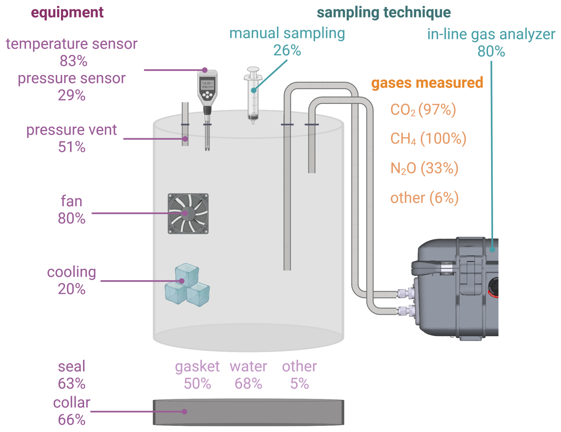
Figure 4 Schematic chamber setup, including the percentage of survey participants using certain types of chamber equipment and sampling approaches for the gas concentrations and for measuring different greenhouse gases. Some participants use both manual sampling and in-line gas analyzer measurements for different applications, research sites, or measurement campaigns, causing the total share of measurement methods used to exceed 100%. Other gases besides CO₂, CH₄, and N₂O, each measured by one survey participant, are ethane and BVOCs (biogenic volatile organic compounds). This figure was created in BioRender.

Pressure vent

A gas flux into or out of a closed chamber would alter the air pressure inside the chamber slowly over time and more rapidly when the chamber is closed. As such a change in pressure can affect the gas flux between soil and the chamber, it is recommended that a vent be installed, constituting a small opening in the chamber that allows for pressure equilibration but that does not allow for significant mixing of ambient air into the chamber to keep the pressure inside the chamber close to the ambient air pressure. Clough et al. (2020) recommend the simultaneous use of two types of vents as they tackle different pressure-related chamber artifacts – a larger one that is open only during chamber placement and a smaller one that remains open during the measurement. Vents for pressure equilibration are only used by half of the participants (Fig. 4). Different methods for pressure equilibration as employed by the respondents were a hole in the chamber that is sealed after chamber placement, explicitly mentioned by two participants, and a long line of tubing that is constantly open to the atmosphere, allowing for pressure equilibration while preventing too much ambient air from entering the chamber, explicitly mentioned by one participant. The responses indicate that the two types of vents are considered to be alternatives for vent designs rather than two measures that tackle different pressure-related chamber artifacts and that should therefore be applied simultaneously. One reason for the low implementation rate of pressure vents could be a fear of causing a so-called Venturi effect, where wind passing over the vent outlet can depressurize the chamber, leading to an increased gas flow from the soil into the chamber (Bain et al., 2005; Conen and Smith, 1998). However, clear guidelines exist on how to avoid the Venturi effect by adjusting the vent design (Xu et al., 2006).

Cooling

Especially in summer, when air temperatures are high, a transparent chamber might act as a small greenhouse, causing the temperature inside the chamber to rise and increasingly deviate from the ambient air temperature over the time of the chamber closure, inducing a temperature gradient between the interior and the exterior of the chamber. A change in chamber temperature should be avoided as it can affect the gas flux by influencing processes like plant processes and evaporation or condensation. About one-fifth of the survey participants address this issue in their chamber setup. As a way to avoid a temperature increase by insulation, 3 % of the participants use opaque or reflecting chambers. Some applications, however, require the use of transparent chambers. This is the case, for example, when determining NEE (net ecosystem exchange). Furthermore, blocking out the incoming radiation can potentially reduce active CH₄ transport through plant aerenchyma, thereby reducing the measured CH₄ emissions (Clough et al., 2020). A total of 17 % of the respondents therefore use active cooling of a non-insulated, transparent chamber. The types of cooling systems mentioned were Peltier elements, circulation of the chamber air through a tank filled with ice water, and fans circulating the cold air from ice packs placed inside the chamber. However, an active cooling of the chamber air bears the risk of overcompensating for a temperature increase and of causing condensation inside the chamber or sampling tubes (Fiedler et al., 2022). It is therefore recommended that active cooling be used only if chamber cannot be insulated and/or if long chamber deployment periods are needed (Maier et al., 2022). The effectiveness of insulation or cooling should be evaluated by comparing surface soil temperatures inside and outside the chambers (Clough et al., 2020).

Chamber pressure and temperature measurements

Recording the temperature and the pressure inside the chamber over the time of the chamber closure is essential for correcting for temperature and pressure using the ideal gas law when calculating CH₄ fluxes, as well as for detecting remaining changes in pressure and temperature over time that could not be eliminated with a pressure vent and insulation or cooling of the chamber headspace. Most participants record the temperature inside the chamber, while only slightly less than one-third of them measure the chamber pressure with measurement frequencies ranging from every second to once per chamber closure. While one temperature and pressure measurement during chamber closure might be sufficient for use in the ideal gas law, higher-frequency measurements are needed in order to consider the stability in environmental conditions inside the chamber as an indicator of flux quality. Only two participants can therefore account for temperature and/or pressure changes over the time of the chamber closure by individually correcting each concentration measurement as they document the chamber temperature and/or pressure at the same frequency as the gas concentrations. Most notably, almost one-fifth of the survey participants do not measure the chamber temperature at all (Fig. 4), which can lead to large uncertainties considering the strong linear effect of temperature on the flux magnitude through the ideal gas law.

Mixing

In the absence of air movement in a closed chamber, a concentration gradient can develop inside the chamber, which might influence the further gas flux between the soil and chamber headspace. A well-mixed headspace is furthermore needed to ensure that a representative gas sample can be taken. While most researchers use fans to mix the air inside their chamber, some researchers argued that the airflow from circulation through a closed loop with the gas analyzer was sufficient to mix the chamber air, such that particularly small chambers did not need a fan. This statement highlights that further research is needed to investigate the strength of turbulence that is adequate for particular chamber dimensions to ensure proper mixing of the chamber air while preventing the artificial release of additional gas from the soil (Christiansen et al., 2011; Maier et al., 2022).

Seal

To reliably quantify the momentary gas exchange between a defined soil surface and the atmosphere, the mixing of chamber air with ambient air needs to be avoided. To achieve this, it is recommended that a chamber base be inserted into the ground to restrict lateral gas transport inside the soil and to additionally ensure an airtight connection between the chamber and its base (Clough et al., 2020). Two-thirds of the participants follow this recommendation and place their chamber on top of a base that they inserted into the ground between 1 h and 1 year before the measurements. The more time that passes between the base insertion and the measurements, the less a potential disturbance of the ground and its concentration gradient will affect the measurements. The fact that the chamber setups employed by one-third of the participants do not involve a collar or a seal might be less problematic than it appears since many participants measure in wetlands or on open water, with the required insertion depth of the chamber into the soil and the necessity of a gastight seal being low under water-saturated conditions and at low soil porosities (Clough et al., 2020). Two-thirds of the participants aim to make the connection between the chamber and the collar or the soil gastight by using one or several types of sealing. Besides gaskets and water seals, a plastic sheet weighed down by a chain, a stocking filled with sand, and foam in the collar groove were mentioned as sealing methods. Every chamber setup should be tested for gastightness before being deployed in the field, as suggested by Clough et al. (2020).

Chamber dimensions

One challenge in developing chamber measurement protocols is to find a balance between a chamber closure time that is short enough to keep the influence of chamber artifacts low but long enough to reach gas concentrations within the chamber headspace that are above the detection limit of the gas analyzer or gas chromatograph used. One way to reduce the minimum time of chamber closure required to exceed the detection limit of the instrument is through reducing the chamber volume.

The volume of the chambers used by the participants ranged from 8 to 1800 L, with a median of 64 L and an interquartile range (IQR) of 105 L. A total of 93 % of the chambers used are smaller than 260 L (Fig. A3). However, more specific recommendations exist regarding the chamber dimensions besides the requirements in terms of its overall volume: to minimize the error caused by potential leakage and to maximize the area sampled, an area-to-perimeter ratio of ≥ 10 cm is recommended, which equates to a diameter of ≥ 40 cm for a cylindrical chamber. Two-thirds of the chambers used by the survey participants respect this recommendation, and the majority (75 %) of chambers with a smaller-than-recommended area-to-perimeter ratio are cylindrical. Furthermore, a ratio of chamber height to deployment time of ≥ 40 cm h⁻¹ is recommended to maximize the flux detection while minimizing the perturbation of environmental variables. This recommendation is followed in 93 % of the measurement setups used by the participants. The two remaining setups had too-long closure times considering the relatively flat chambers. However, flexibility in terms of chamber dimensions and closure times is often limited by the specific conditions of the research site: the minimum closure time needed depends on the flux magnitude of the gas of interest and on the sensitivity of the analyzer, and the chamber height has to be chosen to accommodate the vegetation, while its area might have to be adapted to the surface structure.

Sampling techniques and chamber closure times

Besides reducing the chamber volume, increasing the measurement frequency of the gas concentrations can reduce the required chamber closure time as, in most researched environments, CH₄ emissions are high enough for the minimum detectable flux to be reached rather quickly. Much higher sampling frequencies can be achieved through the use of in-line gas analyzers as opposed to manual sampling of the chamber headspace. The majority of the survey participants use an in-line gas analyzer for continuous and on-site measurements of the gas concentrations inside the chamber (Fig. 4). All but one of these participants employ a closed sample loop which returns the air to the chamber after circulation through the gas analyzer. One participant uses open-path LI-COR gas analyzers installed inside a large chamber. The gas analyzers used by the respondents record the gas concentrations at frequencies of between five times per second and once every 15 s. The chamber measurements therefore use shorter closure times of 0.5 to 12.5 min compared to the closure times of 16 to 50 min used by the fewer participants who manually sample the chamber air every 4 to 10 min (Fig. A4). Two participants using manual sampling keep their chamber closed for more than 40 min, which is considered to be too long by Rochette and Eriksen-Hamel (2008), while earlier guidelines allowed for up to 1 h closure time (Holland et al., 1999). To avoid overly long closure times that promote chamber effects on the measured fluxes, the minimum required closure time should be determined with a consideration of the minimum detectible flux (MDF) based on the sensitivity of the analyzer and the chamber height (Christiansen et al., 2015; Nickerson, 2016).

An additional advantage of in-line gas analyzers over manual sampling, besides reducing the relevance of chamber artifacts through shortening closure times, is that the higher temporal resolution of the gas concentration recordings can reveal remaining chamber artifacts. This enhances the possibilities of evaluating the quality of a flux estimate or of excluding measurement periods affected by chamber artifacts at the stage of flux processing. In-line gas analyzers furthermore allow for the use of chambers that open and close automatically. Such automated chambers are used by one-third of the survey respondents. While being more cost-intensive than manual chambers, automated chambers allow for continuous measurements at a higher temporal resolution.

The precision of the measured gas concentrations might differ between the survey participants as they calibrate their gas analyzers or gas chromatographs at different time intervals: most respondents (58 %) calibrate their instruments once per year, and 24 % do so once before each measurement campaign. A few (10 %) of the participants calibrate the instrument less often, e.g., when serviced every 1 to 3 years, and 12 % calibrate more frequently, ranging from weekly to daily to calibration after each flux measurement.

Reducing anthropogenic disturbance

The survey participants take various precautions to minimize additional disturbances to their chamber measurements that can be caused by the presence of those who measure and by their way of operating the chamber system. For wet, terrestrial sites, 28 participants stand on more stable ground while measuring, either by using permanently or temporarily installed boardwalks or wooden boards or by choosing a drier patch or a rock to stand on. Six participants furthermore mentioned that they make sure not to walk close to the measurement plots by using automated chambers or walking rules supported by warning tape. For aquatic measurements, participants avoid anthropogenic disturbance of the sediment and, thus, of the gas release by pulling the chamber into its measurement location with a rope or by sitting in a boat while measuring. In addition, careful placement of the chamber, training of those who measure, maintenance of collars and sealing, and carefully keeping the vegetation away from the chamber sides were used to minimize disturbances to the chamber measurements.

Ancillary data

Recording additional variables alongside the chamber measurements can help explain the observed gas fluxes, as well as identify potential disturbances to the measurements. The variety of variables measured by the survey participants (Fig. 5) might indicate that, depending on their background and research questions, scientists consider different variables to be important in controlling CH₄ fluxes. Almost all survey participants measure variables to characterize the soil, hydrological, and meteorological conditions, covering most of the ancillary data suggested by Maier et al. (2022). However, the potential effects of the vegetation cover were considered by less than one-sixth of the respondents.

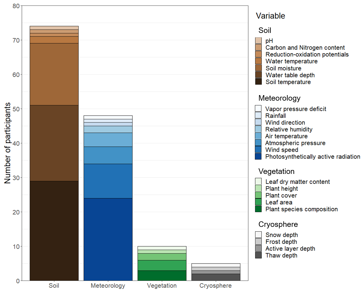
Figure 5 Ancillary data recorded alongside the gas fluxes. Participants were permitted to select multiple variables, allowing the number of responses within one category of ancillary data to exceed the total number of 36 survey participants.

3.1.5 Flux calculation and QC approaches

The qualitative responses regarding the calculation approaches for CH₄ fluxes revealed differences in terms of the flux processing and QC procedures that might result in considerable variation in the CH₄ fluxes among researchers. Gas fluxes are generally estimated from chamber measurements as the slope of the change in gas concentration over the time of the chamber closure and by accounting for the water vapor concentrations, the temperature, and the pressure inside the chamber, as well as for the chamber dimensions. This approach was modified by the survey participants mainly through the selection of a time period of each chamber measurement for flux calculation, by choosing a fit function to estimate the change in concentration over time, and by determining the accuracy of the temperature and pressure correction by selecting a measurement frequency for the two variables or deciding to use standard values instead (Fig. 6). The majority of the participants (90 %) use self-written scripts and functions for their flux calculation, while 20 % of the participants at least partly use existing and published R or MATLAB scripts.

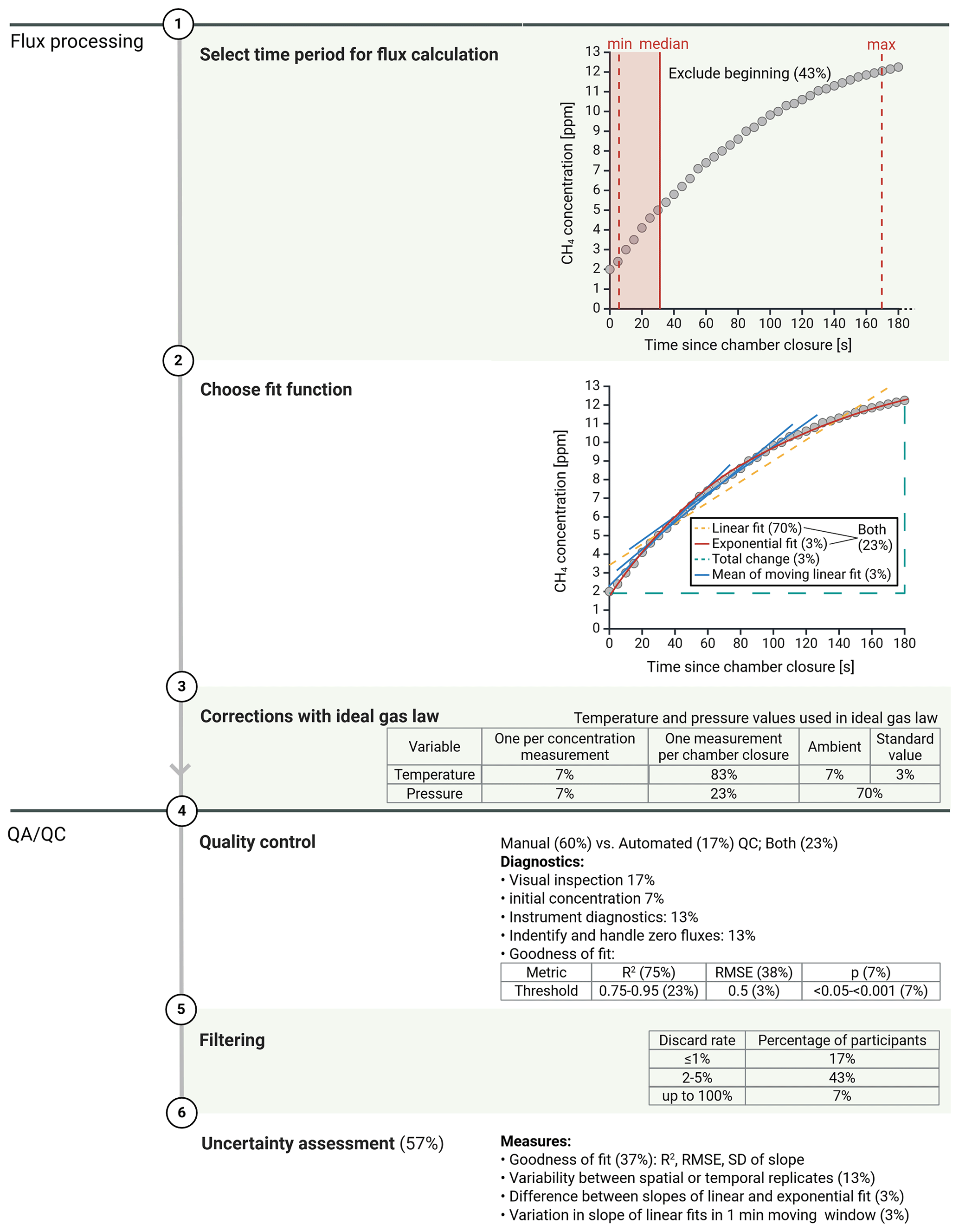
Figure 6 Differences in the workflows used for flux processing, quality control (QC), and quality assurance (QA) by the survey participants. This figure was created in BioRender.

Selecting a time period within a chamber measurement for flux calculation, for many respondents, involves discarding the beginning of each measurement to exclude initial disturbances caused by the chamber placement. Most participants use a linear fit to estimate the change in gas concentration over the time of each chamber measurement. Most remaining respondents compute both a linear fit and the initial slope of an exponential fit, either deciding on one based on the goodness of the fit or using the difference between the two slopes as an uncertainty estimate for the final flux value. Three individual participants use an exponential fit for all chamber measurements, consider the total change in gas concentrations, calculated as the difference between the gas concentrations at the start and at the end of the chamber closure or average multiple linear fits based on a 1 min window moving over the measurement at steps of 10 s, respectively.

In the step of correcting the measured gas concentrations for the temperature and pressure inside the chamber, most participants use one temperature value per chamber closure that is either measured during one point of the chamber measurement or derived as the average of several temperature recordings over the time of the chamber closure. As fewer participants measure the pressure compared to the temperature inside the chamber, more have to rely on ambient pressure recordings or assume standard atmospheric pressure. As opposed to assuming constant conditions over the time of the chamber closure, two participants explicitly stated that they individually correct each gas concentration measurement for the chamber temperature and/or pressure measured at or interpolated to the same frequency as the concentration measurements.

Various approaches for QC of the flux estimates were mentioned by the participants. Most participants manually check each of their chamber measurements, while others use an automated procedure, and some used a combination of both manual and automated diagnosis. Most participants use measures of the goodness of fit to evaluate the quality of their flux estimates, some of whom consider fixed cut-off values of these metrics to decide between keeping or discarding a flux measurement. Apart from two participants, the respondents typically discard up to 5 % of their data.

The uncertainty of each individual flux estimate is assessed by 57 % of the respondents, with most of them using metrics for the goodness of fit or the variability between spatial or temporal measurement replicates. One participant uses the difference between the slopes derived from a linear compared to an exponential fit and another uses the variation in several 1 min linear fits in a moving time window as an uncertainty estimate.

3.2 Results of survey part 2 – visual quality control of a standardized data set

The visual QC exercise revealed that the handling of the measurement examples (decision to keep or discard a measurement and choice of time period for flux calculation) differed between the survey participants depending on their interpretation of the CH₄ concentration change in the chamber headspace over time (Table 1). Furthermore, depending on the shape of the concentration curve (linear or non-linear), the choice of the time period used for flux calculation had a strong impact on the magnitude and, in one case, even on the direction of the estimated CH₄ flux (Fig. 7, Table A2). Detailed descriptions of the individual measurement examples and their handling by the survey participants can be found in Appendix B.

Table 1 Explanations of the overall shape of CH₄ concentrations during chamber closure, reasons to discard, and reasons for and approaches to keeping measurements as given by the participants, as well as the percentage of respondents that kept the measurements and coefficient of variance (CV) of the flux estimates derived from the survey responses by measurement scenario (for details, see Table A2).

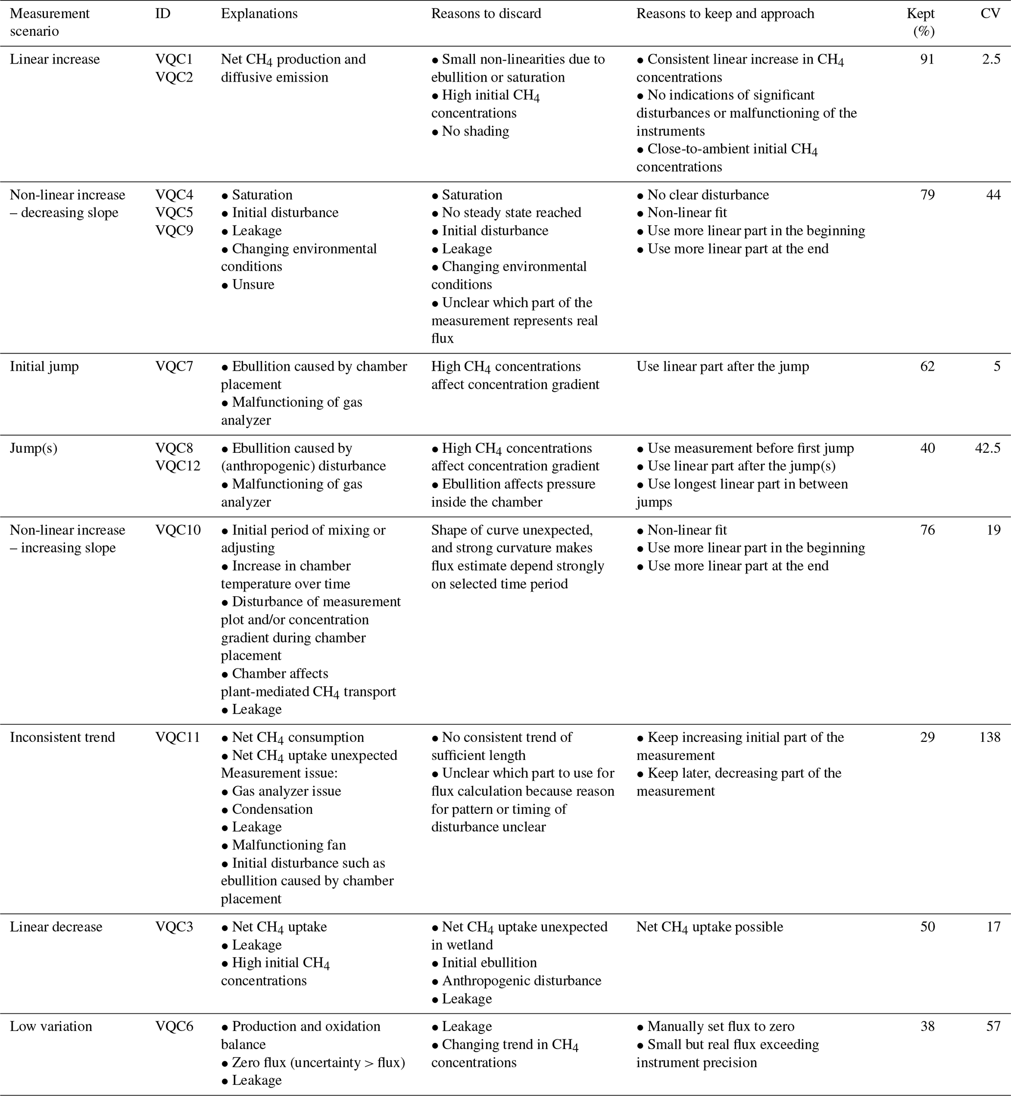
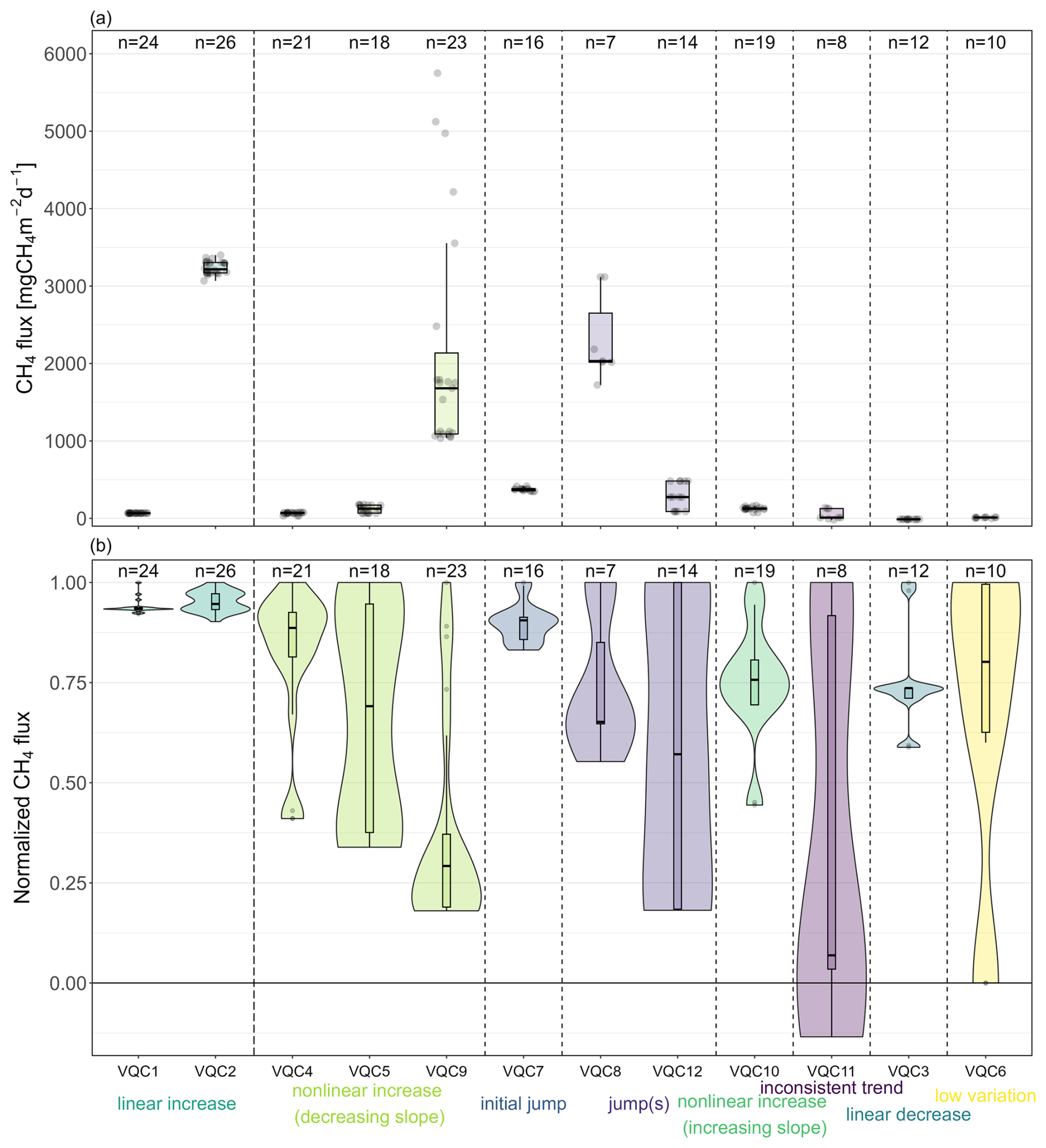
Figure 7 Researcher variability in flux estimates for each measurement example in the visual QC exercise (VQC1–VQC12) by measurement scenario. Range (a) and distribution (b) of flux estimates across the respondents. The number of survey participants (n) who contributed a flux estimate to the respective measurement example by selecting a time period for flux calculation is given on top of each boxplot (a) or violin (b). In (b), the flux estimates are normalized to the maximum flux estimate within each measurement example. The violins are scaled to all have the same maximum width. Violins crossing the zero line indicate that, for the respective measurement example, the selection of the time period for flux calculation made the difference between CH₄ emission and uptake.

3.2.1 Linear fluxes: emission and uptake

The majority of the participants (91 %) decided to keep the measurements that showed a linear increase in CH₄ concentrations for flux calculation. Due to the linear behavior, these flux estimates were the least affected by the time period that was chosen for the linear fit.

The latter also applied to measurement examples showing a linear decrease in CH₄ concentrations over time. However, more participants decided to discard the entire measurement because they did not expect to find net uptake of CH₄ at a wetland site. The free-text responses revealed that the conditions – and, in particular, the water table depths – under which net uptake of CH₄ can occur were debated among the participants.

3.2.2 Non-linear increase – decreasing slope

Most participants (79 %) also kept the measurement examples that showed a consistent but non-linear and weakening increase in CH₄ concentrations over time. Here, the magnitude of fluxes estimated from the non-linear concentration change strongly depended on the time period selected for the flux calculation. The selection of the time period was, in turn, influenced by how the participants explained the observed non-linearity. There were two main lines of reasoning among the participants for their choice of time period, with opposing effects on the flux magnitude: (1) about two-thirds of the explanations for the non-linear behavior assumed that the increase in CH₄ concentrations was weakened by either CH₄ saturation of the chamber headspace or leakage of air from the chamber towards the end of the measurement. The participants concluded that this latter part of the measurement was disturbed and should therefore be excluded from the flux calculation, which resulted in higher flux estimates. (2) Conversely, the remaining third of explanations assumed that the stronger increase in CH₄ concentrations at the beginning of the measurement was caused by an initial disturbance such as ebullition, triggered by the chamber placement. A consequent exclusion of the strong initial increase in CH₄ concentrations from flux calculation resulted in lower flux estimates as the lower slope during the latter part of the measurement was preferentially selected.

3.2.3 Non-linear increase – increasing slope

The survey participants were similarly divided with regard to the appropriate handling of chamber measurements that show a non-linear increase in CH₄ concentrations but with an increasing slope over time. Accordingly, half of the participants who discarded this measurement argued that they cannot justify choosing a time period for flux calculation as they cannot explain the observed shape of the CH₄ concentrations, and, considering the non-linearity, an unsubstantiated selection of a time period could strongly bias the flux estimate. For those who kept the measurement and gave start and end times for flux calculation (65 % of participants), the time period chosen significantly affected the flux estimate. This range between higher and lower flux estimates again resulted from contrasting explanations regarding the non-linear concentration change: higher flux estimates originated from explanations assuming an initial period of adjustment and disturbance caused by the chamber placement through exclusion of the initial, lower slope in CH₄ concentrations. On the other hand, explanations involving chamber effects on CH₄ cycling processes through alteration of environmental conditions or interference of CH₄ measurements with high H₂O concentrations led to lower flux estimates due to the exclusion of the stronger increase in CH₄ concentrations towards the end of the measurement.

3.2.4 Jumps

The majority of the respondents (65 %, 88 %, 92 %) interpreted the jumps shown in three of the measurement examples as episodic events of ebullitive CH₄ emission, while one participant suggested a malfunctioning of the gas analyzer. The survey responses revealed uncertainty around the question of under which water table conditions CH₄ ebullition is most likely to occur, indicating a fundamentally different understanding of the causes of ebullition events among the participants. There were two major considerations concerning CH₄ ebullition during chamber measurements: first, the survey participants disagreed on whether ebullition events should be included in flux estimates from chamber measurements or if diffusive and ebullitive fluxes should be quantified separately, either by isolating periods of ebullitive and diffusive flux in one concentration time series or by separately measuring ebullition, for example, using bubble traps. When accounting for both diffusive and ebullitive CH₄ emissions by using a linear fit over an entire measurement containing ebullition events, as suggested by 4 % to 8 % of the participants, flux estimates were up to 5 times as high as the ones considering the diffusive flux only. Second, the respondents disagreed on whether the remaining part of a measurement after an ebullition event could still be used to quantify the diffusive flux. More than half of the survey participants (54 %) kept the linear part of a measurement after an initial ebullition event for flux calculation, while 38 % of the participants discarded the entire measurement. The latter assumed that the high CH₄ concentrations in the chamber following the ebullition event would decrease the concentration gradient and thus reduce the CH₄ flux between the soil and chamber headspace for the rest of the measurement. This decision also influenced the range of flux estimates derived from a measurement with repeated ebullition events. Flux estimates from the 15 % of participants who used a shorter linear increase in CH₄ concentrations before the first ebullition event were 3 times as high as the flux estimates from the 19 % of participants who fitted the longer linear increase after the first ebullition event.

3.2.5 Low variation

Another source of uncertainty in data handling among the survey participants lay in the identification and handling of so-called zero fluxes. Two-thirds of the survey participants discarded the measurement example showing only very low variation in CH₄ concentrations without a clear trend over the time of the chamber closure. The other third of the participants submitted a flux estimate, 20 % of whom set the flux to zero, while 80 % calculated the small positive flux resulting from a non-linear fit. One participant remarked that the magnitude of CH₄ variations would need to be compared to the instrument precision to decide on whether a measurement can be classified as a zero flux.

3.2.6 Inconsistent trend

Less than one-quarter of the respondents kept the measurement example showing a reversing trend in CH₄ concentrations over the course of the measurement. Of all the measurement examples, the resulting flux estimates varied most strongly between the participants in this case, that is, by more than the mean flux value and including both positive flux estimates and one negative flux estimate. This indicates that, in cases where the trend in CH₄ emissions changes between an increase and a decrease over the time of the measurement, interpretations of the concentration time series can make the difference between net CH₄ emission or uptake.

3.2.7 Further considerations

The survey participants repeatedly mentioned several other reasons to discard a measurement besides an overall non-linear or otherwise unexpected behavior in CH₄ concentrations. These reasons included too-high initial gas concentrations, assumed leakage of air from the chamber headspace, and a too-short measurement time. Furthermore, some participants considered the simultaneously measured H₂O and CO₂ concentrations as additional indicators of measurement quality: non-linear or otherwise unexpected behaviors, as well as high initial concentrations of H₂O and CO₂, were mentioned as reasons to discard a measurement. Similarly, interference of CH₄ measurements with high H₂O concentrations towards the end of a measurement was mentioned several times as an explanation for non-linear behavior in CH₄ concentrations. Linear changes in CO₂ and H₂O, on the other hand, were considered to be proof of the airtightness of the system. To avoid the impact of any initial disturbance caused by the chamber placement on the flux estimate, almost half of the survey participants, by default, excluded the beginning of each measurement (30 ± 85 s (median ± IQR)) from their flux calculations.

3.2.8 Effect of different flux calculations on an example flux data set

Using the prevalence of different measurement scenarios in the Siikaneva data set (Table A1), we estimated an overall variability in the calculated CH₄ fluxes due to differences in terms of the time periods used for fitting, as well as an overall variability in the inclusion and/or exclusion of measurements. Different researchers chose different parts of the same measurement for flux calculation (Figs. B1–B12), which resulted in an overall flux difference of 17 % across the Siikaneva data set (Table A2). The variation in the percentage of measurements in the Siikaneva data set passing the visual QC was 28 % (Tables 1 and A2). This estimated variability introduced by the selection of different time periods for flux calculation compares with the mean natural temporal variability of 19 % but is lower than the mean natural spatial variability of 88 %, calculated from automated chamber measurements of CH₄ fluxes in five temperate and Arctic peatlands by Pirk et al. (2016). Similarly, Pirk et al. (2016) found that the natural spatial and temporal variabilities in CH₄ fluxes exceed the difference between fluxes estimated using different fit functions. However, it must be noted that the uncertainty estimates derived in our study consider only the effect of differences in terms of visual QC and do not account for different measurement setups or different fit functions used for flux calculation, both of which can add variability to fluxes (e.g., Pihlatie et al., 2013).

4 Evaluation of the survey methodology

4.1 Expert survey approach and insights

For our study, we used the method of an expert survey, which allowed us to combine the accuracy of a literature review with the directness of an expert assessment. In general, a literature review might provide a more complete overview of the methods used and, thus, allow for more reliable statistical interpretation of the results. However, we found that published data sets and research articles involving chamber fluxes often lacked detailed information on measurement and data handling procedures – one of the current hurdles in interpreting, reusing, and combining existing chamber flux data sets. The expert survey, on the contrary, allowed us to obtain specific information directly from the scientists – information which might not be available in published literature but that might, nonetheless, significantly affect the CH₄ fluxes estimated from chamber measurements. In designing our survey, we had somewhat limited examples to follow as the approach of an expert survey rather than an expert assessment is not commonly employed. While the exact implementation of the survey could therefore surely be refined in future studies, we showed that surveying experts on their methods can be a useful approach and that this is strongly complementary to earlier reviews and recommendations regarding best measurement practices (e.g., Clough et al., 2020; de Klein and Harvey, 2012; Fiedler et al., 2022). The survey results clearly reveal that agreement on the measurement setup is high and generally in line with recommendations (Fig. 4), but strong variability in the flux estimates is introduced at the data processing and analysis stages by the different researchers (Fig. 7, Table A2). This provides an opportunity to re-focus the discussion from measurement setups and linear vs. exponential fitting approaches to a wider discussion about data workflows and uncertainty sources in chamber flux measurements that have emerged with new observational methods.

4.2 Representativeness of the survey respondents and questions

From the variety of survey responses, it becomes clear that evaluating the representativeness of the respondents of the chamber flux community as a whole is challenging. One reason for this is that the chamber flux measurement community remains less organized than the eddy covariance flux measurement community and is more fluid, potentially because the barriers to entry, i.e., the cost of analysis, are lower. We recruited the survey participants from different places of employment assuming that this would make them rather independent in terms of their choice of measurement and data handling approaches. The main strength of the collected data set therefore lies in representing a large range of measurement and data handling practices; indeed, there were substantial deviations in workflows within the part of the chamber flux community represented in this survey (Figs. 4 and 6). However, we did not reach all researchers using chamber fluxes with our survey; we likely underrepresented those working in agricultural ecosystems, disturbed sites, and tropical ecosystems. Overall, participants who had not encountered a certain shape in CH₄ concentrations in their own data sets before were more likely to discard the respective measurement example (Tables 1 and A2). For example, the measurement showing decreasing CH₄ concentrations over time was discarded by 50 % of the current participants (Table 1), many of whom focus on wetland ecosystems (Fig. 3), but this measurement is more likely to occur in well-drained agricultural soils (Mosier et al., 1997). Thus, the background of the survey participants might have affected the outcome of the visual QC exercise, with a bias towards expected (higher) fluxes.

Additionally, the question of the number of survey participants is always a concern. While the number of researchers contacted (n= 46) and the final maximum of 36 respondents might seem relatively low for a community survey, we estimate that this still represents a considerable fraction of an estimated total number of several hundred chamber flux experts world-wide. Time is always a factor in voluntary survey participation; therefore, it was important to streamline questions to incentivize survey completion. In offering diverse question types, we attempted a balance between making the responses comparable and categorizable among the participants while still obtaining detailed information on their reasoning for the use of specific measurement and data handling techniques. The limited number of survey participants required a low number of possible responses in choice questions to allow for a meaningful statistical interpretation of the survey results; therefore, we used yes-or-no answers rather than scales of agreement. Yes-or-no questions further allowed us to draw conclusions on the prevalence of the implementation of recommended best measurement practices among the survey participants.

4.3 Assumptions in the flux calculations: site and researcher differences

Our estimates of researcher variability in flux data sets, derived from the visual QC exercise, strongly depended on the underlying reference data set collected at Siikaneva bog (Table A1). Both natural processes and chamber-induced artifacts occur, and their prevalence depends on both the environmental conditions of the research site and the chamber design and measurement setup. Most measurements in the Siikaneva data set (∼ 60 %) showed the linear increase in CH₄ concentrations that is expected for undisturbed measurements at a wetland site. However, a non-linear, weakening increase in CH₄ concentrations was also represented by a rather high share of measurements (18 %) and is also regularly observed at other sites (e.g., Pirk et al., 2016). The survey responses confirm that it is often unclear whether this shape is caused by an initial disturbance of the measurement or by CH₄ saturation of the chamber headspace over time (Table 1). Furthermore, this lack of process understanding shows through in the high variance associated with the non-linear fluxes (Fig. 7, Table A2). An initial disturbance, i.e., ebullition caused by the chamber placement, was a common explanation (Table 1) and might have occurred more frequently in the Siikaneva data set than at other sites as roughly 60 % of the measurements were obtained from vegetation removal plots. The removal of vascular plants and of the Sphagnum moss layer might have reduced both plant-mediated CH₄ transport and CH₄ oxidation, resulting in higher CH₄ concentrations in the pore water and, thus, increasing the probability of ebullition events (Jentzsch et al., 2024a). While CH₄ ebullition is a natural phenomenon often encountered in wetlands (Green and Baird, 2013), the increased probability of both natural and anthropogenically induced ebullition due to vegetation removal might have contributed to the high share of measurements (16 %) showing abrupt jumps in CH₄ concentrations in the Siikaneva data set.

Although some measurement scenarios included in the visual QC exercise are relatively uncommon, it is still important to evaluate how these scenarios would be handled by different researchers as they were shown to be large sources of disagreement (Table A2). Many survey participants stated that the non-linear increase in CH₄ concentrations with an increasing slope over time was unexpected. However, this shape was reported surprisingly often in other studies and occurred during several of our measurements (Table A1). Overall, this behavior of CH₄ concentrations in the chamber headspace is not consistent with diffusion theory (Kutzbach et al., 2007), indicating the influence of other processes. Similarly, both low changes in CH₄ concentrations without a clear trend and a decrease in CH₄ concentrations over time occurred infrequently in the Siikaneva data set (< 1 % of measurements) but were scenarios with high variability in the calculated fluxes (Table A2). Still, small fluxes might be expected at higher and drier wetland microtopographical features (e.g., Laine et al., 2007), while low, close-to-zero fluxes and/or CH₄ uptake are more commonly observed at upland sites (Virkkala et al., 2024; Voigt et al., 2023).

Overall, the Siikaneva data set might have contained more non-linear measurements than data collected by the survey participants due to the selected experimental setup, as well as site-specific environmental conditions. This theory is difficult to test as this information is not often available for other sites but might be a reason for the high discard rate in the visual QC exercise. While the median percentage of measurements that the researchers said they discarded from their own data sets was 5%, they discarded 19 % in the visual QC exercise when weighted by the prevalence of measurement scenarios within the Siikaneva data set (Tables A1 and A2). Another reason for the high discard rate might be that the survey participants did not do the measurements themselves. They did not have the option to redo a measurement that they diagnosed as disturbed, and they lacked an overall view of the data set. Several participants mentioned that they would like to see the entire data set before deciding on keeping or discarding an individual measurement as they did not know the prevalence of the different measurement scenarios; the decisions for processing an entire data set might differ from the limited number of example measurements presented here. Processing the full data set as a common data set rather than just a small subset would also eliminate the assumptions made with the visual classification of measurement scenarios (Table A1); however, this might also have decreased the number of respondents as this is a relatively intensive exercise. If respondents did their own flux calculations, this would allow for non-linear fitting methods, which we did not use in our exercise despite this being occasionally suggested by a participant (7 % of responses). While our fitting and calculation approaches may have been overly simplistic, post hoc assumptions regarding how many participants would have used a non-linear fit and the different fitting options (such as exponential, quadratic, or logarithmic functions) would introduce substantial additional uncertainty into our estimates of researcher variability. Reproducing the calculation approaches of every respondent would have required additional, very detailed information from the survey participants, likely reducing the number of completed surveys and, thus, making our uncertainty estimates less representative of the entire chamber flux community. However, this type of exercise might be worth undertaking in the future.

5 Visions for improving chamber CH₄ flux measurements and data sets

5.1 Recommendations for high-frequency measurements of CH₄ fluxes from chambers

Earlier studies have highlighted variability in CH₄ fluxes due to chamber design and fitting approaches (e.g., Fiedler et al., 2022; Maier et al., 2022; Pihlatie et al., 2013; Pirk et al., 2016). Here, we show that many researchers have adopted the recommended measurement techniques and setups (Fig. 4). The relatively widespread adoption of high-frequency CH₄ analyzers provides new challenges and illustrates a need to move the focus from the measurement setup and curve-fitting considerations to data handling as the disagreement in QC approaches varies widely among the survey participants, and explanations for some observed behaviors remain inconsistent (Tables 1 and A2). While broader discussions about QC approaches are warranted, some simple steps may help to improve data quality.

1. Calculation and implementation of a minimum detectable flux given the analyzer precision and chamber height. This could be used to determine the measurement length and to determine when fluxes are below the detection limit. Short measurement times should be used to avoid chamber effects.

2. Not discarding fluxes, including ebullition fluxes, low fluxes, or zero fluxes. Instead, we should move towards a standardized QC flagging system. Ebullition fluxes and low and zero fluxes should be preserved and can be flagged in archived data. CO₂ concentrations can be used in addition to CH₄ concentrations to determine measurement quality (Pirk et al., 2016). This will work best in dark chambers as a net emission is expected. H₂O vapor is less reliable as an indicator of flux quality.

3. Reporting all data for archival purposes and implementing data quality flagging. A flagging system will indicate to others that are interested to re-use the data where uncertainties lie and has been implemented in eddy covariance networks. Ideally, raw concentration data will be archived, along with processed data. This will allow for the reprocessing of data in the future as needed.

In the longer term, we need to develop new tools and networks to figure out how we can best leverage the new possibilities resulting from high-frequency gas concentration measurements. Key steps are underway to allow for easier operation, analysis, and standardization of flux calculations, for example, the goFlux package for R (Rheault et al., 2024). In earlier times, ebullition was difficult to identify using gas chromatography (GC) analysis but can now be seen in the high-frequency concentration time series (Figs. B6–B8), allowing for the separation of ebullition from diffusive fluxes (e.g., Hoffmann et al., 2017). The survey showed strong disagreement with how to handle these measurements, sometimes resulting in quite large variations in flux magnitude (Fig. 7), suggesting that this new insight into CH₄ transport pathways is not fully utilized. Overall, more discussion and exploration of this crucial measurement approach are needed to fully leverage the technological developments of the past decade.

5.2 Establish a formal trace gas chamber flux network

One reason for the large variability in chamber methods revealed in this survey could be a lack of exchange between the researchers working with chamber measurements of CH₄ fluxes. Only half of the survey participants are part of a flux monitoring network, such as FLUXNET or AmeriFlux, both of which focus strongly on eddy covariance measurements. This indicates that the exchange within the chamber flux community might be impeded by a lack of suitable networking platforms. Chamber-technique-focused conference sessions and workshops to further develop approaches and revise methodologies would be beneficial. Further discussion and recommendations toward a more rigorous standardization of flux calculations by identifying the best fit based on objective criteria (e.g., Pedersen et al., 2010; Rheault et al., 2024) would be the domain of such a network. While much work has already gone into developing chamber-based approaches and recommendations for measurements, the substantial (and potentially novel) uncertainty in fluxes calculated among researchers shown here indicates that this matter is not yet settled (Fig. 7). Furthermore, there was never complete agreement on whether to keep or exclude the fluxes included in the survey (Table 1).

Introducing a chamber flux network and data platform might speed up the adoption of a more standardized measurement protocol (although many recommended chamber components are widely adopted; see Fig. 4); improve metadata and ancillary measurement quality; spur the development of a data quality flagging system that could foster a transparent exchange between researchers with regard to measurement and data handling procedures; and, ultimately, enhance the compatibility of individual flux data sets. Such a chamber flux network could build on existing research infrastructures such as the LTER sites, the ICOS sites in Europe, and the NEON sites in North America. Some examples for chamber databases have been developed, like the Soil Respiration Database (SRDB), which includes chamber measurements of ecosystem respiration and has been widely cited, particularly for the response of ecosystem respiration to warming (Bond-Lamberty and Thomson, 2010a, b; Jian et al., 2021). This requires the open sharing of data, including both the raw chamber measurements and the calculated flux estimates using quality flagging rather than pre-filtered flux data sets. This way, reanalysis of existing data sets can be facilitated, and all chamber measurements contributing to larger-scale synthesis studies can be reprocessed using a uniform calculation and QC approach to remove differences among researchers, which, as we have shown, significantly affect CH₄ flux estimates (Fig. 7).

5.3 Development and adoption of tools for uncertainty estimation in data processing

We demonstrated the potential of using a common data set to assess the variance in flux estimates caused by different data processing and QC approaches (Fig. 7). This approach could also be implemented more broadly to build consensus on calculation methods, quality control, and data quality indices. The survey participants performed a detailed quantitative and qualitative evaluation of example measurements and explained the decisions they made with regard to data handling (Fig. 6). This helps to identify differences in the rationale for the processing and QC approaches they used; these differences affect fluxes, even in the small number of example fluxes in this survey (Fig. 7). The resultant variability in fluxes could be assessed in a more rigorous way by distributing an entire data set of raw chamber measurements to flux experts and the community as a whole to process using their own calculation and QC approaches. Using a common data set could provide a more accurate estimate of the uncertainty due to data processing by different researchers and could add insights into the relevance of this additional source of variability in CH₄ fluxes through comparison with the natural spatial and temporal variability in the data set. Sharing an entire data set would also eliminate some assumptions made in terms of data processing in this survey (Sect. 4.3). The fluxes estimated from the raw data set could then be uploaded to a chamber flux network website or an existing platform, such as GitHub, to add to a growing pool of flux data sets computed from the same chamber measurements by different researchers. A flagging metric could be added to indicate data quality, which would aid modelers and others in interpreting and understanding noisy observations, which are common in ecosystems with high spatial and temporal heterogeneity. This way, every interested researcher could assess how the flux estimates based on their processing techniques relate to those calculated by other flux experts and could help to build agreement on how to handle unclear cases of non-linear concentration changes.

Additional synthetic data could be an important addition to chamber measurements in the reference data set and would clarify the processes resulting in strongly divergent flux estimates (Fig. 7). A forward model could be developed to simulate the change in CH₄ concentrations in a chamber headspace as the real flux overlaid by a combination of chamber-induced artifacts in response to environmental conditions (Hutchinson and Livingston, 2001). This way, researchers could compare their flux estimates to the known “real” flux underlying a simulated measurement to see if they succeed in detecting it against background noise and artifacts.

Measurement simulations can also help to understand how CH₄ (and co-varying CO₂) concentrations change in response to commonly cited measurement issues that might result in non-linear fluxes (Table 1). The simulations can therefore answer the key questions that appeared in the visual QC exercise: which part of a non-linear measurement should be used for flux calculation? Can the linear part of a measurement following an ebullition event still be used for flux calculation? How should close-to-zero fluxes be identified and handled? Does a decrease in headspace CH₄ concentrations indicate actual CH₄ uptake? Pirk et al. (2016) demonstrated that applying a non-linear model for flux calculations can lead to an overestimation of CH₄ emissions if the non-linear change in CH₄ concentrations was not, as assumed, caused by a change in the gas concentration gradient over time. Improved process understanding will help to avoid introducing bias into flux data sets through unsubstantiated handling of non-linear measurements.

Models and experimental studies to assess the effect of instrumentation on the flux estimates have previously been used to derive guidelines for certain aspects of measurement setups, such as chamber dimensions, pressure vents, and airtight seals (Christiansen et al., 2015, 2011; Hutchinson and Livingston, 2001; Pumpanen et al., 2004). Additionally, model-derived metrics can be used in post hoc quality control, as was demonstrated for the minimum detectible flux (MDF) metric by Nickerson (2016). Such metrics will help identify a standardized set of required metadata with regard to the chamber setup and experimental design, as well as ancillary measurements that should be taken alongside CH₄ fluxes in addition to the various variables currently recorded for the specific applications of the survey participants (Fig. 5). For example, using a model with inputs of the air–soil CH₄ concentration gradient in the soil together with soil porosity and other soil properties can help to assess the potential effect of headspace saturation on the CH₄ flux (Pirk et al., 2016), which was commonly cited as problematic in this analysis (Table 1). Introducing model-derived metrics will therefore help scientists to make more informed decisions when selecting a time period within a chamber measurement for flux calculation, choosing a fit function, and filtering the data set. From the metrics, one can derive diagnostics for quality flagging that foster standardization of quality control procedures while factoring in site-specific conditions.

6 Data availability

The results of the expert survey described in this paper are available from PANGAEA: https://doi.org/10.1594/PANGAEA.971695 (Jentzsch et al., 2024b).

7 Conclusions

Chamber flux measurements are crucial for capturing spatial variability in ecosystems and for quantifying treatment effects on greenhouse gas emissions. At broader spatial scales, synthesis data sets of chamber CH₄ fluxes show differences among but also high variability within wetland classes (Kuhn et al., 2021; Treat et al., 2018). The high variability within classes has been attributed to high spatial and temporal variability and can be partly compensated for by using longer integration times (Treat et al., 2018) or by capturing spatial variability due to microtopography effects (Virkkala et al., 2024). The results from this expert survey show that differences in terms of methodology may be an additional factor contributing to high variability in CH₄ fluxes across sites and data sets. For example, the handling of low positive and negative fluxes can significantly affect estimates of CH₄ budgets, particularly in high-latitude and upland regions where low CH₄ emissions and/or uptake of CH₄ can be expected during large parts of the year. Discarding low or zero fluxes can lead to a bias towards higher CH₄ emissions and potentially result in the difference between a net annual uptake or a net emission of CH₄ in low-flux regions. Ebullition events may also comprise a substantial fraction of emissions; discarding these may lead to an underestimation of ecosystem CH₄ fluxes.

Our assessment of flux variability points towards the questions of where and when we introduce the largest error into our flux estimates: is it when we choose our measurement setup and processing approaches or do the location and the timing, together with the spatial and temporal resolution of the measurements, matter more? Answering this question will help identify the most relevant starting points for improving the accuracy of flux estimates and will help lower uncertainties in flux syntheses. In any case, the survey shows that our human decision-making introduces uncertainties that can obscure natural spatial and temporal variability in CH₄ fluxes. This might make it harder to identify relevant spatial and temporal environmental drivers of CH₄ fluxes, which is crucial for model development and CH₄ budget estimations.

Appendix A

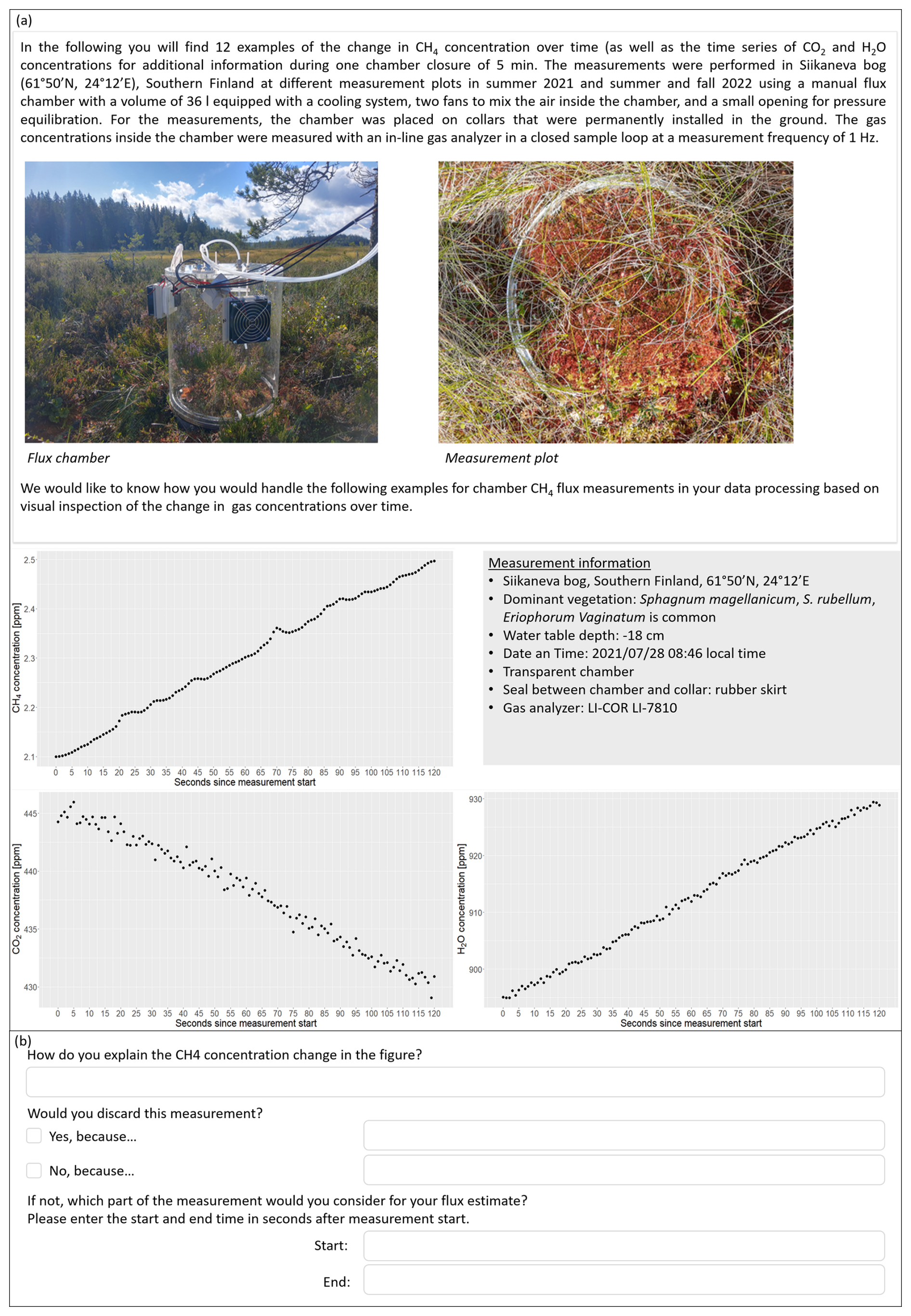
Figure A1 Example of the information provided (a) and the questions asked (b) for the visual QC of 1 of the 12 chamber measurements under discussion.

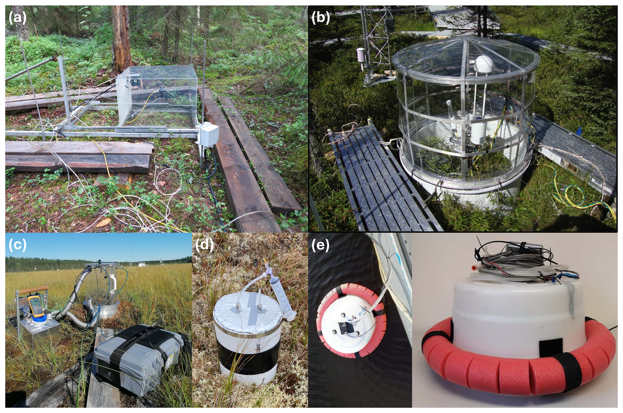
Figure A2 Examples for different chamber setups in different environments. Automated chamber in a boreal forest (a), large manual chamber with gas analyzer inside the chamber (b), transparent manual chamber with in-line gas analyzer and cooling unit in a boreal fen (c), opaque manual chamber with a syringe for manual gas sampling and a tube for pressure equilibration (d), and floating chamber connected to in-line gas analyzer and deployed from a boat for aquatic measurements (e).

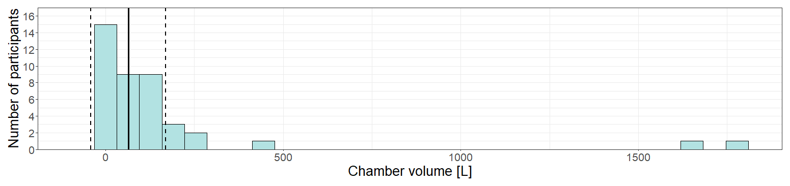
Figure A3 Histogram of the chamber volumes. The solid lack line denotes the median, and the dashed black lines denote the IQR.

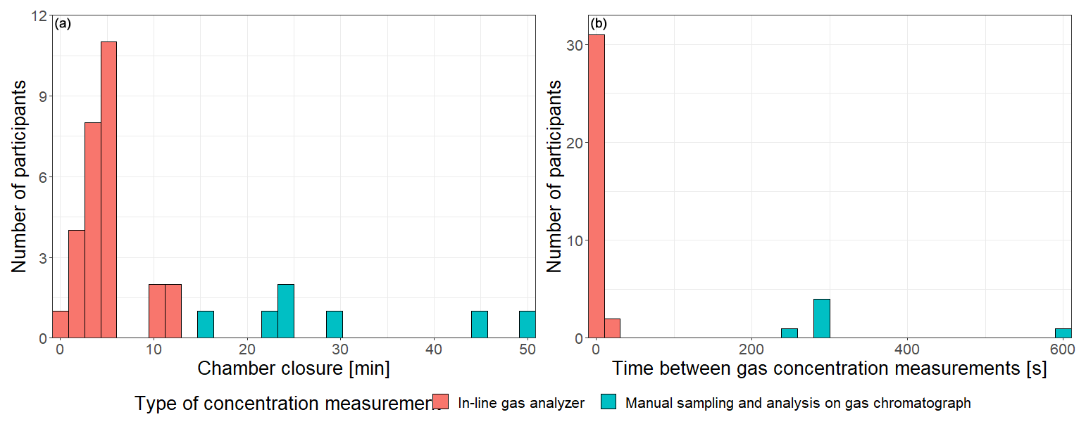
Figure A4 Duration of chamber closure (a) and frequency at which the gas concentration inside the chamber is recorded as the time between two measurements (b) by type of concentrations measurement.

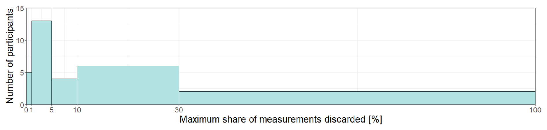
Figure A5 Maximum percentage of measurements that the survey participants usually discard from their own data sets.

Table A1 Number and percentage of occurrence of identified measurement scenarios in a data set of chamber measurements collected at Siikaneva bog, southern Finland, in 2021 and 2022. Categorization of the 12 measurement examples used in the visual QC exercise into these measurement scenarios and weighting factors calculated for each measurement example for the extrapolation of CVs derived from the 12 measurement examples to a representative data set (Table A2). Weighting factors were derived as the relative occurrence of the respective measurement scenario in the Siikaneva data set (788 measurements in total) divided by the number of occurrences in the visual QC exercise.

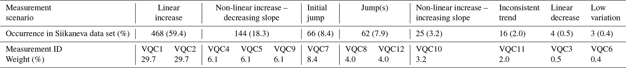
Table A2 Visual QC exercise: fluxes (in mg CH₄ m⁻² d⁻¹) calculated for each example chamber measurement (columns) by each survey participant (rows) based on the time periods chosen for flux calculation in the visual QC part of the survey. Coefficients of variance (CVs) are given for each example measurement (CV_ex) and each measurement scenario (CV_scenario) across the participants. NR indicates that a participant did not respond to the respective measurement example and so neither kept nor discarded the measurement, and D indicates that a participant discarded a measurement example. Percentage of measurements kept for flux calculation: percentage of measurement examples within the visual QC exercise kept for flux calculation by participant (kept_VQC, relative to total number of measurement examples that a participant responded to), measurement example (kept_ex), and measurement scenario (kept_scenario). Extrapolation to Siikaneva data set and uncertainty estimates: extrapolation of the visual QC results to the entire Siikaneva data set through weighting by the frequency of occurrence of each measurement scenario in the data set (Table A1). Answers from participants who gave no response to more than one measurement example were excluded from the calculations of kept_VQC and kept_Sii, indicated by NA (not available). Participants who did not participate at all in the visual QC exercise have been excluded from the table.

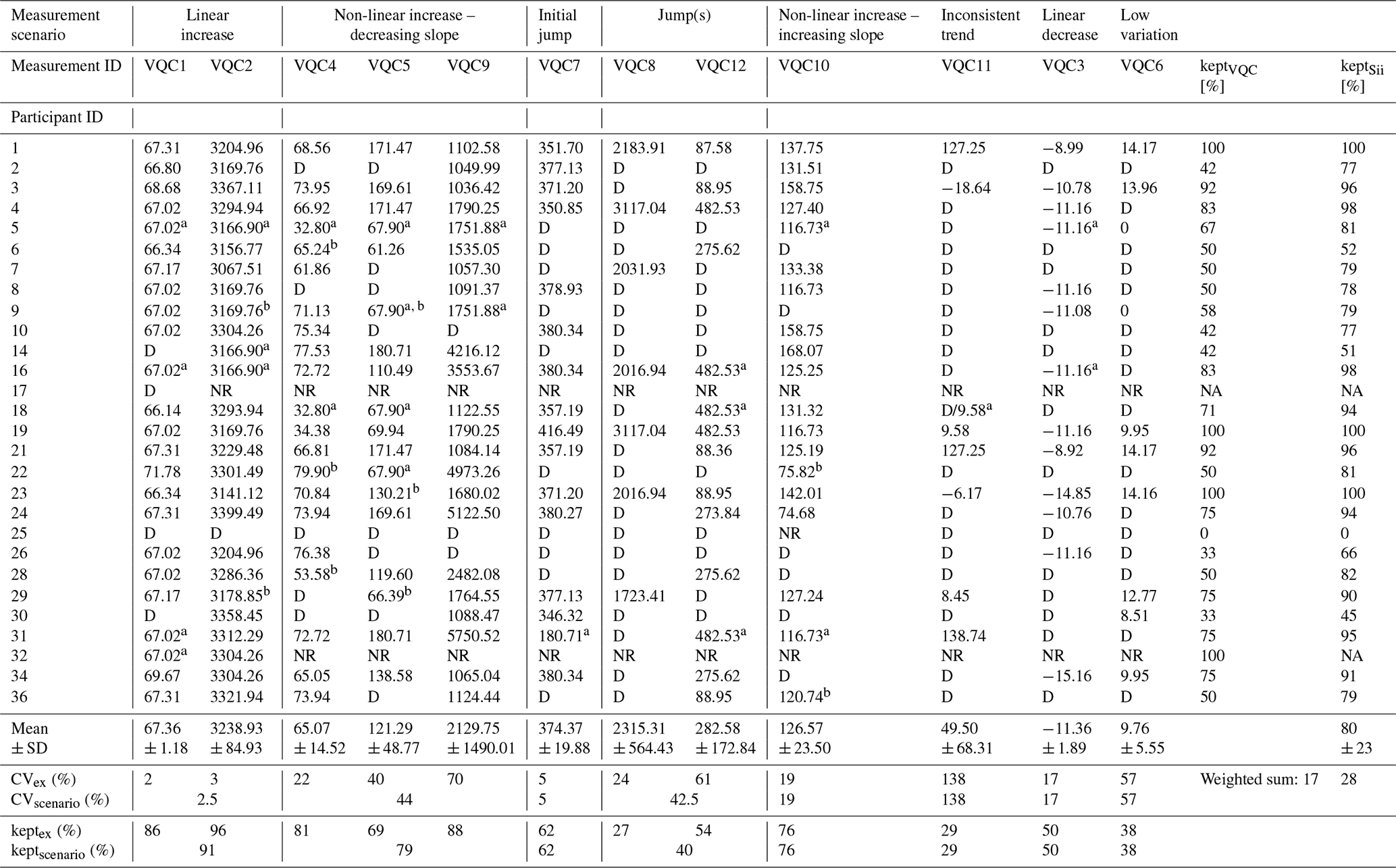
^a Accepted, but no time period was given for flux calculation. The flux was therefore estimated based on the entire measurement.
^b Flux was estimated based on a linear fit, although the participant suggested using a non-linear model instead.

Appendix B

B1 Linear increase

Two example measurements included in the visual QC exercise showed a linear increase in CH₄ concentrations over the entire time of the chamber closure. In the first example (measurement ID VQC1, Fig. B1), the CH₄ concentrations increased by only 0.4 ppm from a starting concentration of 2.1 ppm to a concentration of 2.5 ppm at the end of the measurement, while, in the second example (measurement ID VQC2, Fig. B2), the starting concentration of 3.8 ppm was higher and increased by 38.2 ppm to reach 42.0 ppm over the course of the measurement. The CO₂ concentration in the chamber decreased during both measurements by 13.4 and 9.1 ppm, respectively. The starting concentration of H₂O in VQC2 was more than 10 times higher than that in VQC1 and decreased strongly over the course of the measurement, with an abrupt decrease at around 50 s after chamber closure, while H₂O concentrations increased slightly in VQC1.

The participants described the trend in CH₄ concentrations in both VQC1 and VQC2 as a linear increase, which they explained referring to net CH₄ production and diffusive emission. The CH₄ flux in VQC2 was additionally classified as large, with one participant concluding that the measurement plot was a “hotspot” for CH₄ emission. For both VQC1 and VQC2, some participants also noticed slight deviations from the linear behavior of the CH₄ concentrations. Minor jumps in the CH₄ concentration in VQC1 were mentioned by 17 participants (61 %), which they related to CH₄ ebullition (9 participants), insufficient mixing due a defective fan (3 participants), wind (1 participant), wind-induced pressure changes (1 participant), changes in atmospheric pressure influencing the ground diffusion rates and/or the atmospheric pressure gradient (1 participant), boundary layer disturbance (1 participant), leakage (2 participants), and disturbance (1 participant) caused by chamber placement or footsteps (1 participant). For VQC2, half of the participants pointed out a decrease in the slope of CH₄ concentrations starting between 250 and 260 s after the chamber closure, 21 % of whom also noticed a simultaneous decrease in the slope of CO₂ concentrations. As explanations, the participants mentioned saturation of the chamber headspace decreasing the concentration gradient over time (five participants); a build-up of pressure (two participants) potentially due to a defective pressure valve towards the end of the measurement (one participant); a change in temperature over the course of the measurement (one participant); or a small leak (one participant), probably combined with windy conditions (one participant). Furthermore, many participants discussed the change in CO₂ and H₂O concentrations over the time of the chamber closure. For VQC1, three participants mentioned that the CO₂ and H₂O concentrations show a linear change, two of whom concluded that there was no air leaking from the chamber. On the other hand, three participants were concerned about the H₂O measurements due to the high and increasing concentrations and due to an assumed saturation and, therefore, a decreasing slope towards the end of the measurement. Leakage from the chamber was suspected by three participants, two of whom explained this presumption with vegetation overgrowing the collar and one of whom explained this presumption with the use of a less airtight rubber seal as opposed to a water seal. For VQC2, 18 % of the participants picked up on the drop in H₂O concentrations occurring around 40 s after the chamber closure, 40 % of whom additionally mentioned a simultaneous change in the slope of CO₂ concentrations. Their reasoning included water condensing on the chamber walls and changing light conditions. Only a few participants decided to discard the two measurement examples. Measurement VQC1 was discarded by four participants (14 %) who suspected CH₄ ebullition or stated that the starting concentrations of CO₂ were too far above ambient concentrations or that all chamber measurements generally need to be shaded. One participant excluded VQC2 due to an assumed saturation effect, and one additional participant mentioned ebullition and a high initial concentration of CH₄ as potential reasons to exclude the measurement from flux calculations. Totals of 86 % and 89 % of the participants decided to keep VQC1 and VQC2 for flux calculation, respectively, due to the consistent linear increase in CH₄ concentrations without clear indications of significant disturbances or any malfunctioning of the instruments. For VQC1, the participants further supported their decision with the fact that the linear change in CO₂ and H₂O concentrations makes leakage from the chamber unlikely, as well as with near-ambient CH₄ concentrations at the measurement start. For both VQC1 and VQC2, most participants who gave start and end times for flux calculation chose the middle part of the measurement, discarding the beginning and the end without mentioning a specific reason. The remaining participants considered the CO₂ and/or H₂O concentrations in their choice of the time period for curve fitting. For VQC1, three participants chose the beginning of the measurement only, resulting in slightly higher flux estimates, two of whom assumed that H₂O saturation diminished the increase in CH₄ concentrations towards the end of the measurement. For VQC2, some participants acknowledged the strong drop in H₂O concentrations. Having no further information regarding potential reasons, three of them decided not to let this unexpected behavior in H₂O concentrations make them discard the CH₄ measurements, while other participants reacted by excluding the time of the drop in H₂O concentrations from their calculation of the CH₄ flux by using the part of the measurement either after the drop (seven participants) or before the drop (one participant). A total of 61 % of the 23 participants who entered start and end times for flux calculation discarded the end of the measurement where CH₄ and CO₂ concentrations increased at a lower rate, resulting in slightly higher flux estimates above 3200 mg CH₄ m⁻² d⁻¹. Two participants suggested using a non-linear fit, with one of them specifying that it should be exponential.

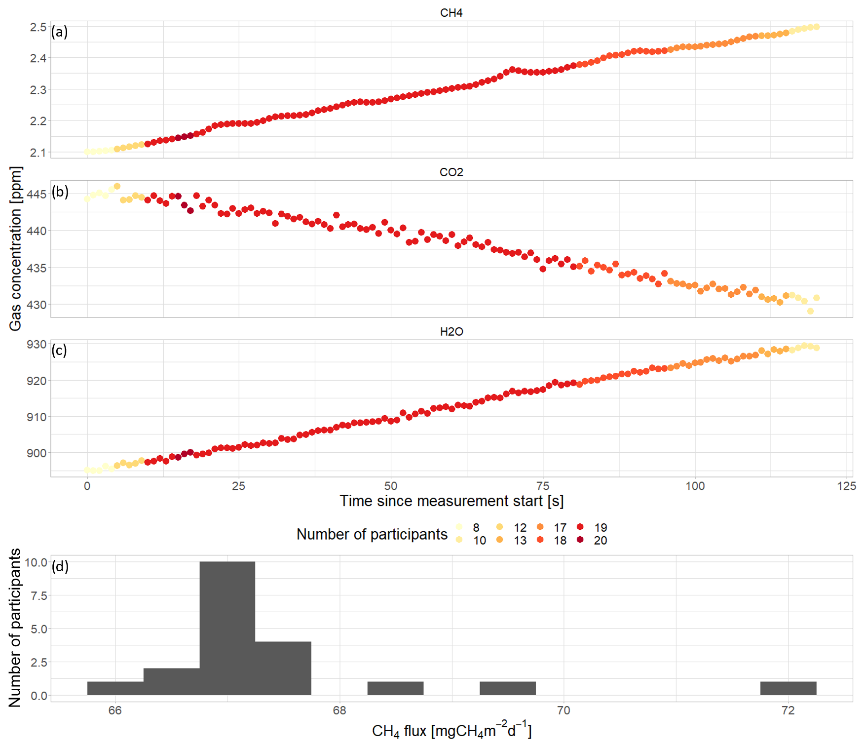
Figure B1 Measurement example (VQC1) of a small linear increase in CH₄ concentrations over the time of the chamber closure. Simultaneous measurements of CH₄ (a), CO₂ (b), and H₂O (c) concentrations over time during chamber closure, with the colors of the data points indicating how many participants included the respective data point in the time period that they chose for flux calculation. Only the responses by participants who gave start and end times for flux calculation were considered for this figure. Histogram of CH₄ fluxes calculated based on the time period chosen by the participants for flux calculation (d).

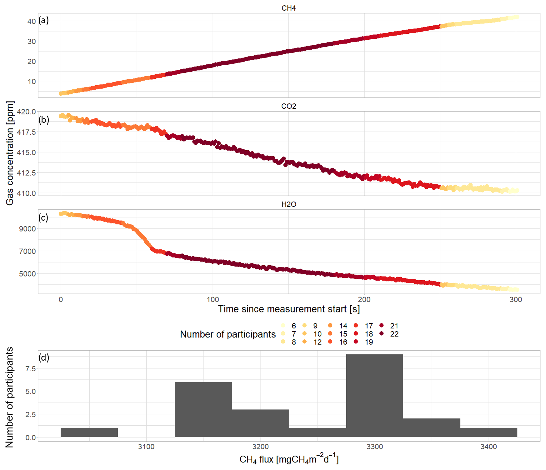
Figure B2 Measurement example (VQC2) of a strong linear increase in CH₄ concentrations over the time of the chamber closure. Simultaneous measurements of CH₄ (a), CO₂ (b), and H₂O (c) concentrations over time during chamber closure, with the colors of the data points indicating how many participants included the respective data point in the time period that they chose for flux calculation. Only the responses by participants who gave start and end times for flux calculation were considered for this figure. Histogram of CH₄ fluxes calculated based on the time period chosen by the participants for flux calculation (d).

B2 Non-linear increase – decreasing slope

In the visual QC exercise, we included three examples of measurements that feature a non-linear increase in CH₄ concentrations during the chamber closure, with the rate of increase flattening out over time. Two examples show a small non-linear increase in CH₄ concentrations (measurement IDs VQC4 and VQC5, Figs. B3 and B4) that occurs simultaneously with linearly decreasing CO₂ concentrations. H₂O concentrations increased over the time of the chamber closure in VQC4 but decreased in VQC5. The third example (measurement ID VQC9, Fig. B5) shows a stronger increase in CH₄ concentrations with intermittent jumps, linearly increasing CO₂ concentrations, and H₂O concentrations that fluctuate without a clear trend.

The participants classified the CH₄ measurement in VQC5 as a small flux that resulted from a balance between CH₄ production and oxidation, while that in VQC9 was identified as large emission indicating a CH₄ hotspot. The majority of the participants (85 %, 85 %, and 81 %) discussed the non-linear behavior of the CH₄ concentrations in VQC4, VQC5, and VQC9, respectively, offering various explanations for the decreasing rate of the increase over time that were mainly related to chamber saturation, chamber leakage, or an initial disturbance (Table B1).

Most participants (9, 10, and 8) suspected a saturation of the chamber headspace, while two participants stated that saturation was unlikely to be reached during a measurement as short as VQC4 (330 s), and one participant explicitly mentioned that the changing slope in VQC9 did not look like a saturation effect. Just as many participants (nine) suggested leakage through a weakening seal as the reason for the decreasing slope in VQC4, as supported by the simultaneously decreasing slope in CO₂ and H₂O concentrations, while other participants explicitly stated that CO₂ and H₂O concentrations did not indicate a leak in this measurement. Due to the consistently linear CO₂ concentrations in VQC5 and VQC9, singular participants suspected leakage during each of these measurement examples. For VQC4, three participants further suspected that the high H₂O concentrations at the end of the measurement influenced the CH₄ measurements, for example, through condensation inside the chamber or in the gas flow line; one participant suggested a varying performance of the chamber fan; and two participants assumed that the non-linearity was a phenomenon specific to Sphagnum moss. One participant more generally suggested that vegetation effects changed over the course of the measurement due to changing light conditions, affecting the CO₂ and H₂O concentrations in VQC4 and the CH₄ concentrations in VQC5.

Besides a saturation effect or a weakening seal that would cause a decreasing slope in CH₄ concentrations towards the end of the measurement, many participants (three, six, and eight) suggested that an initial disturbance such as ebullition triggered by the chamber placement had caused the stronger increase in the beginning of measurement examples VQC4, VQC5, and VQC9. For VQC9, 31 % of the participants additionally pointed out minor fluctuations superimposed onto the overall non-linear increase in CH₄ concentrations. Two-thirds of them referred to the fluctuations as minor ebullition events, while the others suggested episodic leakage from the chamber potentially caused by gusts of wind lifting the chamber sides or a malfunctioning pressure gauge. One participant pointed out that the CH₄ fluctuations co-occurred with fluctuations in the H₂O concentrations and therefore suspected an instrument issue that could be related to spikes in the instrument cavity pressure.

The non-linearity in the CH₄ concentrations resulted in 15 %, 31 %, and 12 % of the participants deciding to discard the entirety of measurement examples VQC4, VQC5, and VQC9, respectively (Table B1). The reasons mentioned for the exclusion of the measurements again reflected the different interpretations of the participants regarding which part of the measurement represented the real flux. This disagreement is shown less strongly in the range of flux estimates since participants who suspected an initial disturbance of the measurement often discarded the entire measurement as they assumed that an initial disturbance would also affect the remaining part of the measurement. For VQC4 and VQC5, all 54 % of the participants who provided start and end times for flux calculations agreed that the beginning of the measurement should be used for or at least be included in the flux calculation, with three participants suggesting a non-linear fit for both measurement examples. This resulted in smaller ranges of flux estimates compared to VQC9 (Table B1), which, instead, reflects the fundamentally different interpretations among the participants regarding which part of the measurement should be used for flux calculation. Here, half of the 21 % of participants who gave start and end times for flux calculation chose a later part of the measurement where CH₄ concentrations appeared to be linear over a longer time period. This resulted in lower flux estimates (between 1000 and 1200 mg CH₄ m⁻² d⁻¹) compared to the flux estimates larger than 3500 mg CH₄ m⁻² d⁻¹ derived for the one-quarter of participants who, instead, chose the beginning of the measurement (Fig. B5).

Table B1 Explanations for the non-linear increase in CH₄ concentrations, reasons to discard, and reasons and ways to keep measurements showing an increase in CH₄ concentrations as given by the participants. The responses were categorized based on the free-text entries for measurement examples VQC4, VQC5, and VQC9. The number of responses given in the respective category is provided in brackets.

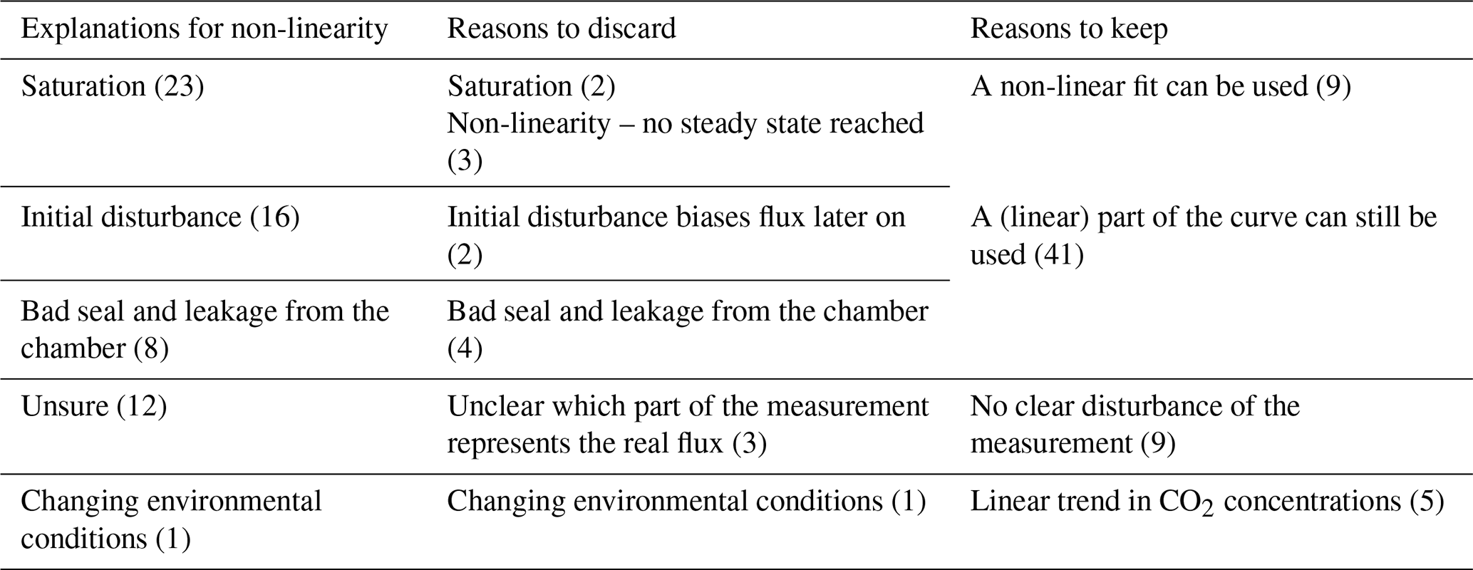
Figure B3 Measurement example (VQC4) of a small non-linear increase in CH₄ concentrations, with decreasing slope over the time of the chamber closure. Simultaneous measurements of CH₄ (a), CO₂ (b), and H₂O (c) concentrations over time during chamber closure, with the colors of the data points indicating how many participants included the respective data point in the time period that they chose for flux calculation. Only the responses by participants who gave start and end times for flux calculation were considered for this figure. Histogram of CH₄ fluxes calculated based on the time period chosen by the participants for flux calculation (d).

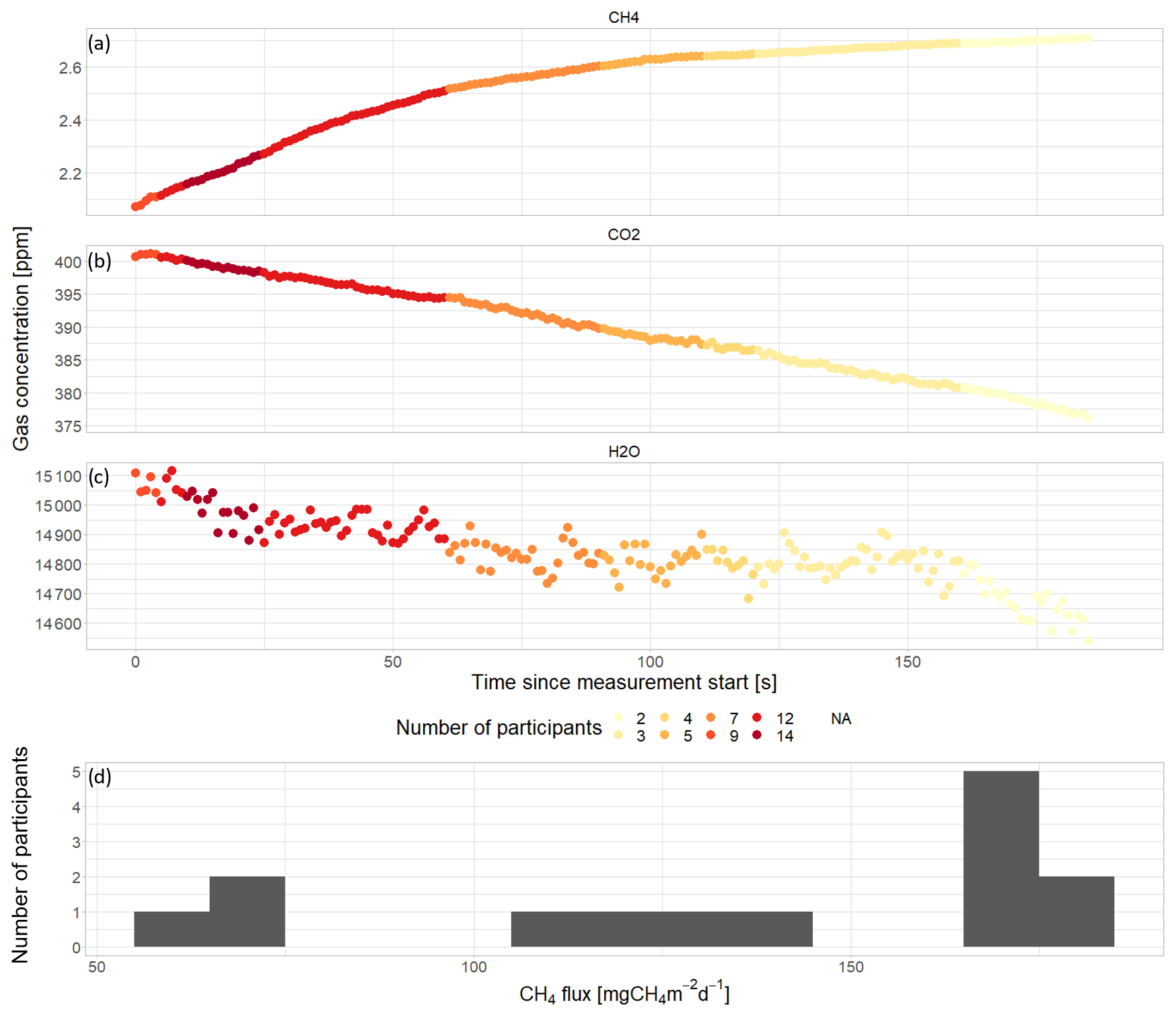
Figure B4 Measurement example (VQC5) of a small non-linear increase in CH₄ concentrations, with decreasing slope over the time of the chamber closure. Simultaneous measurements of CH₄ (a), CO₂ (b), and H₂O (c) concentrations over time during chamber closure, with the colors of the data points indicating how many participants included the respective data point in the time period that they chose for flux calculation. Only the responses by participants who gave start and end times for flux calculation were considered for this figure. Histogram of CH₄ fluxes calculated based on the time period chosen by the participants for flux calculation (d).

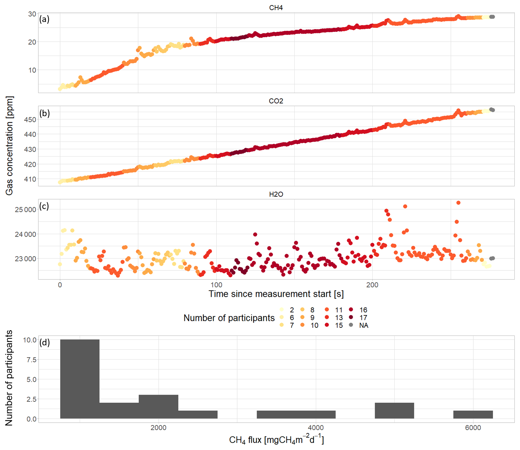
Figure B5 Measurement example (VQC9) of a strong non-linear and jumpy increase in CH₄ concentrations, with decreasing slope over the time of the chamber closure. Simultaneous measurements of CH₄ (a), CO₂ (b), and H₂O (c) concentrations over time during chamber closure, with the colors of the data points indicating how many participants included the respective data point in the time period that they chose for flux calculation. Only the responses by participants who gave start and end times for flux calculation were considered for this figure. Histogram of CH₄ fluxes calculated based on the time period chosen by the participants for flux calculation (d).

B3 Jump(s) at the beginning or in the middle of measurements

In our visual QC exercise, we included three example measurements that showed a relatively linear increase in CH₄ concentrations that was interrupted by one (VQC8, Fig. B6, and VQC7, Fig. B7) or more (VQC12, Fig. B8) sudden increases in the concentration. In one, this occurred at the beginning (VQC7), and, in the others, this occurred in the middle of the measurement (VQC8, VQC12). In examples VQC8 and VQC7, these sudden jumps appeared in all three gases, with CH₄ and H₂O concentrations showing a sudden increase, while CO₂ concentrations dropped simultaneously. In VQC12, on the contrary, CO₂ and H₂O showed no equivalent to the jumps in the CH₄ concentration. In VQC8, a strong decrease in CH₄ concentrations directly followed the sudden increase, while, in VQC7 and VQC12, the concentrations continued to increase at a lower rate, starting close to the high concentration level after the jump.

Nearly all (100 %, 65 %, and 92 %) of the participants mentioned the jump(s) in CH₄ concentration when discussing the measurement examples VQC8, VQC7, and VQC12, respectively. For all measurement examples, the majority of these participants explained their observations with episodic events of ebullitive CH₄ emission (VQC8: 65 %; VQC7: 88 %; VQC12: 92 %), with singular participants suggesting, for VQC7 and VQC12, a malfunctioning of the gas analyzer as a reason for the sudden increase in CH₄ concentrations. Some (35 %) of the participants assuming ebullition stated that the ebullition event in VQC8 was caused by a disturbance, and all agreed that the chamber placement caused the ebullition for VQC7. Only one participant (5 %) mentioned anthropogenic disturbance as the reason for the ebullition events in VQC12. For VQC8, 12 % of the participants pointed out the sudden changes in CO₂ and H₂O concentrations, along with the jumps in CH₄. The reasons mentioned by one participant each were a malfunctioning of the gas analyzer and an overpressure caused by the bubble release, while another participant suggested the release of gas bubbles with high CH₄ but low CO₂ concentrations as a natural cause for this observation. Similarly, one of the two participants who mentioned the absence of a simultaneous change in the other gases in VQC12 assumed a release of bubbles with high CH₄ concentrations but CO₂ concentrations close to ambient conditions due to the different production depths of the two gases. For VQC8, 41 % of the participants discussed the decrease in CH₄ concentrations following the assumed ebullition event and suggested leakage of air from the chamber, potentially combined with wind, as a potential cause. In the discussion of VQC7, two participants disagreed on the effect of the water table on CH₄ ebullition, with one mentioning that, in the measurement, CH₄ ebullition was more likely to happen because of the high water table, while the other stated that ebullition happened despite the high water table, indicating a fundamentally different understanding of the causes of CH₄ ebullition among the participants. Furthermore, two participants of VQC7 classified the measurement as an example of strong CH₄ emission, which they explained with the strong anaerobic CH₄ production related to the high water table and with the vegetation providing a substrate for acetoclastic CH₄ production, respectively.

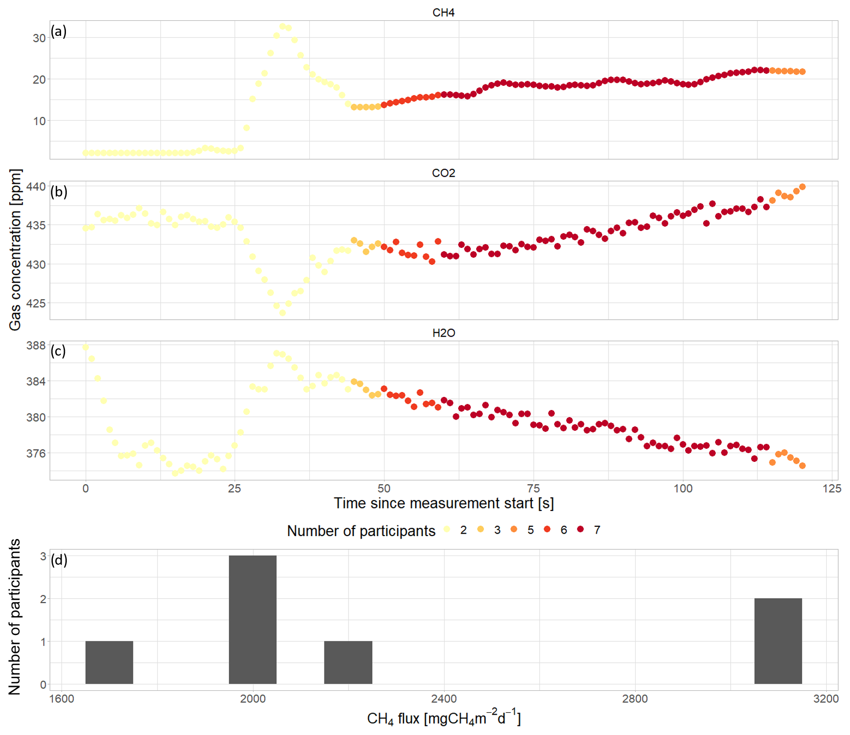
Figure B6 Measurement example (VQC8) of an overall increase in CH₄ concentrations over the time of the chamber closure after a strong jump in CH₄ concentrations. Simultaneous measurements of CH₄ (a), CO₂ (b), and H₂O (c) concentrations over time during chamber closure, with the colors of the data points indicating how many participants included the respective data point in the time period that they chose for flux calculation. Only the responses by participants who gave start and end times for flux calculation were considered for this figure. Histogram of CH₄ fluxes calculated based on the time period chosen by the participants for flux calculation (d).

Of the three measurements with jumps in the CH₄ concentration that we included in the visual QC exercise, VQC8 raised the most concern, with the highest number of participants excluding the example (Table A2) and with the largest variety of reasons mentioned for the discard, including the inconsistent trend in CH₄ and CO₂ concentrations, making the participants wonder which part of the measurement to use for flux calculation; ebullition affecting the pressure inside the chamber; too much variation in the CH₄ and CO₂ concentrations, even after the jump; chamber leakage; and too-high initial CH₄ and CO₂ concentrations. For VQC7, leakage was also suggested by one participant, who suspected that Sphagnum moss might have obstructed the chamber seal with the collar. VQC12 was classified as too short of a measurement by one participant and was discarded by another for too-high initial CO₂ concentrations.

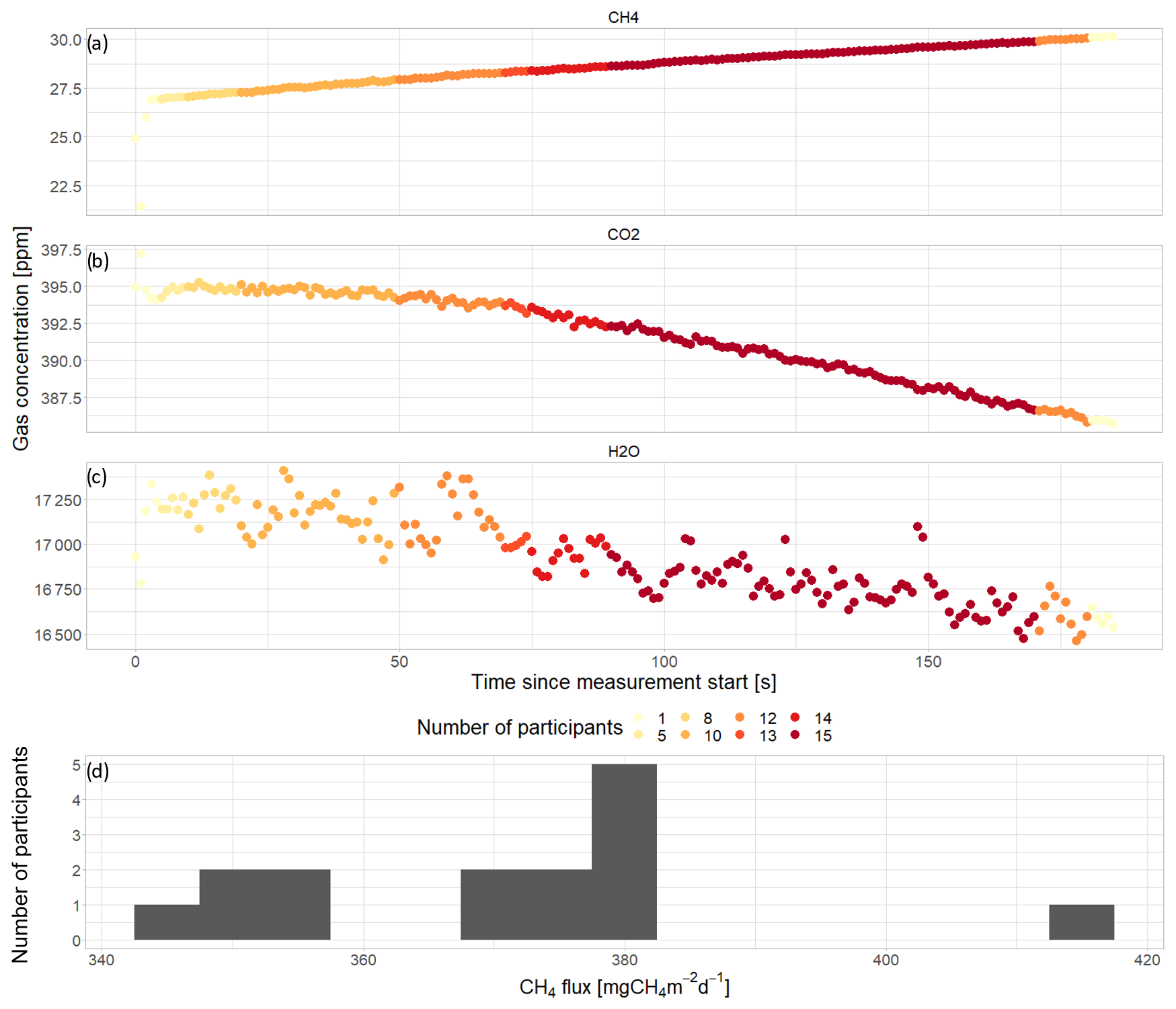
Figure B7 Measurement example (VQC7) of a linear increase in CH₄ concentrations of the chamber closure after an initial jump in CH₄ concentrations. Simultaneous measurements of CH₄ (a), CO₂ (b), and H₂O (c) concentrations over time during chamber closure, with the colors of the data points indicating how many participants included the respective data point in the time period that they chose for flux calculation. Only the responses by participants who gave start and end times for flux calculation were considered for this figure. Histogram of CH₄ fluxes calculated based on the time period chosen by the participants for flux calculation (d).

There was disagreement among the participants on whether the remaining part of a measurement after a jump in the CH₄ concentration could still be used for flux calculation. For 10 out of the 11 participants discarding VQC7, the main concern was high concentrations having a lasting effect on the concentration gradient and, thus, on the diffusive CH₄ flux during the rest of the measurement, while only 1 out of 21 and 15 participants discarded measurements VQC8 and VQC12 for that reason. For VQC12, 4 out of the 11 participants who kept the measurement, all of whom also gave start and end times, avoided this problem by using the beginning of the measurement before the first jump for flux calculation. On the contrary, for VQC8 and VQC7, 5 and 14 out of the 7 and 15 participants who kept the measurement and/or gave start and end times for flux calculation decided that the measurement after the jump in CH₄ concentrations could still be used for flux calculation, and 5 participants in VQC12 preferred to use the part between the first two jumps because it showed a longer linear increase.

The choice of different time periods for flux calculation resulted in two and three different classes of flux magnitudes for VQC8 and for VQC7 and VQC12, respectively. The highest flux estimates of more than 3000, 483, and 416 mg CH₄ m⁻² d⁻¹ stemmed from the two, one, and two participants who used the whole of the measurement examples VQC7, VQC8, and VQC12, respectively, for flux calculation because these estimates also included ebullitive emissions in addition to diffusive CH₄ emissions, reflecting the general disagreement on whether CH₄ ebullition should be directly included in the flux estimates derived from chamber measurements. For VQC7 and VQC12, the flux estimates from the participants who excluded the jumps in CH₄ concentrations from the time period for flux calculation can be further split into two classes. For VQC7, nine participants excluded only the very beginning of the measurement, while five participants only used a later part, starting at about 50 s into the measurement, when CO₂ concentrations decreased at a higher rate, resulting in slightly lower CH₄ fluxes. For VQC12, when excluding the jump in CH₄ concentrations, the flux estimates were higher for four participants who chose the measurement period before the first jump, reaching up to 275 mg CH₄ m⁻² d⁻¹, compared to the five participants who chose the longest linear part of the measurement, leading to fluxes as low as 88 mg CH₄ m⁻² d⁻¹. Due to the very linear behavior of the CH₄ concentrations following the initial jump and the higher agreement regarding the time period used for flux calculation, the CV of 5 % for VQC7 was much lower than the CVs of 24 and 61 % for VQC8 and VQC12, respectively.

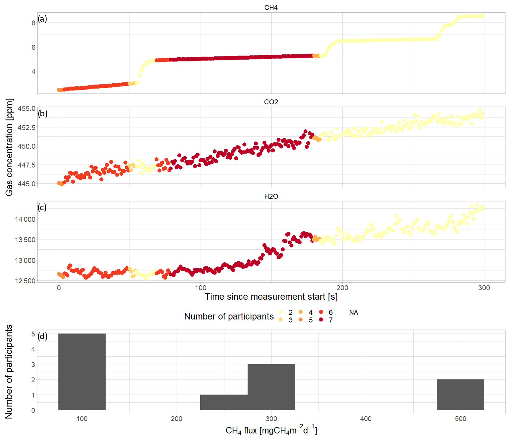
Figure B8 Measurement example (VQC12) of a linear increase in CH₄ concentrations between repeated jumps in the CH₄ concentration over the time of the chamber closure. Simultaneous measurements of CH₄ (a), CO₂ (b), and H₂O (c) concentrations over time during chamber closure, with the colors of the data points indicating how many participants included the respective data point in the time period that they chose for flux calculation. Only the responses by participants who gave start and end times for flux calculation were considered for this figure. Histogram of CH₄ fluxes calculated based on the time period chosen by the participants for flux calculation (d).

B4 Non-linear increase – increasing slope

One example included in the visual QC exercise showed a non-linear increase in CH₄ concentrations over the chamber closure, with the rate of increase becoming stronger over time (measurement ID VQC10, Fig. B9). A total of 15 % of the participants classified the measurement as a diffusive emission of CH₄ without mentioning further details, while 65 % discussed the increasing slope in CH₄ concentrations over time, suggesting various reasons that could have caused the observed shape of the curve. The reasons suggested included an initial period of mixing or adjustment, an increase in chamber temperature over time, a disturbance of the measurement plot, a disturbance of the concentration gradient in the soil during chamber placement, an influence of the chamber on plant-mediated CH₄ transport, an incomplete sealing of the chamber, incomplete mixing, and an interference with the simultaneously increasing H₂O concentrations. Two participants mentioned that they had not seen such a shape in CH₄ concentrations from chamber measurements before. Regarding the magnitude of CH₄ emissions, three participants pointed out the strong increase in CH₄ concentrations despite the relatively low water table, which they related to plant-mediated CH₄ transport. One participant further mentioned that the emission of CO₂ was also high, indicating warm peat conditions. Two participants mentioned the higher and decreasing CO₂ concentrations in the beginning of the measurement, which one of them related to the chamber placement, pushing more gases out of the ground. Furthermore, one participant mentioned that the chamber seal seemed to be intact.

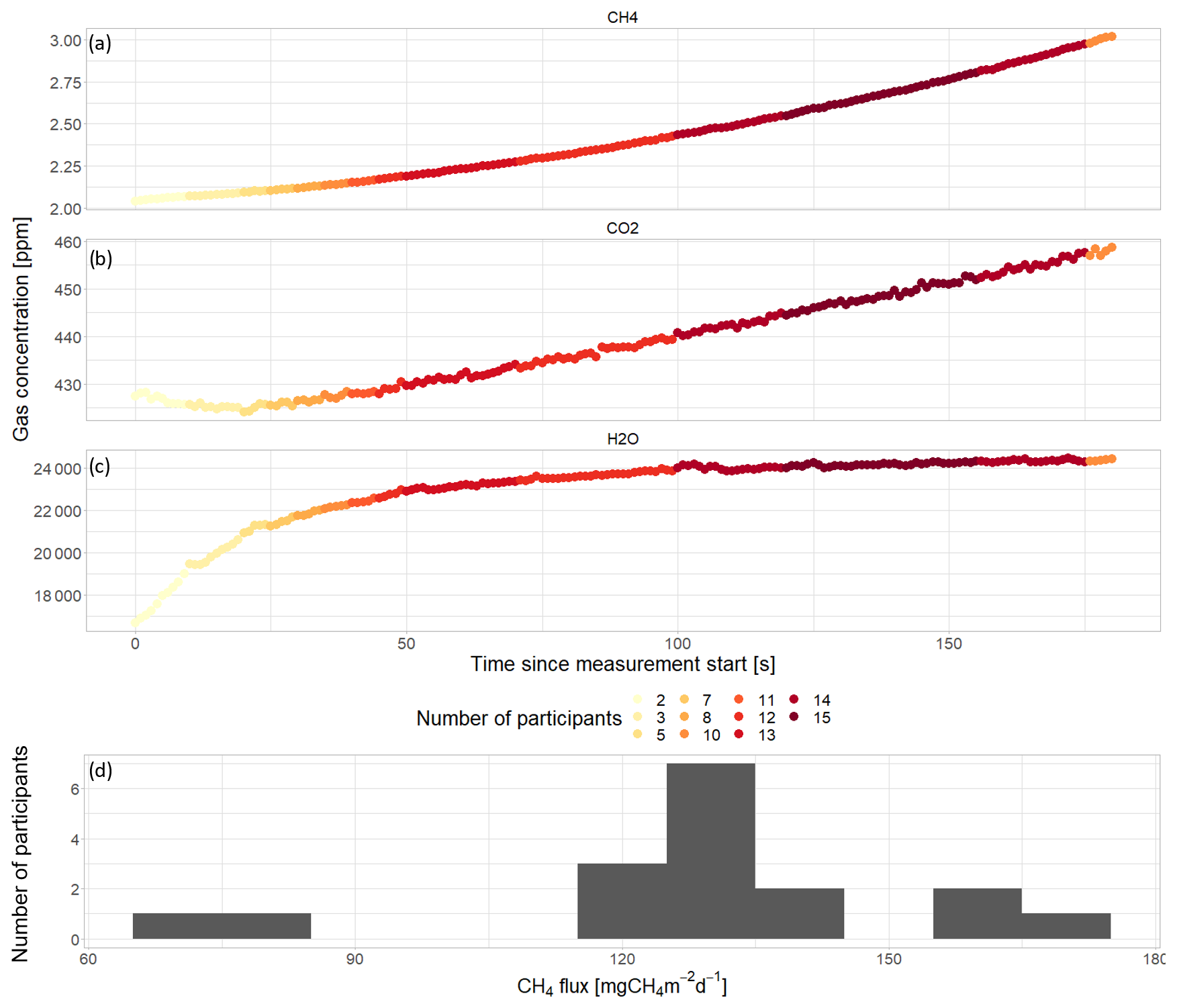
Figure B9 Measurement example (VQC10) of a small non-linear increase in CH₄ concentrations with increasing slope over the time of the chamber closure. Simultaneous measurements of CH₄ (a), CO₂ (b), and H₂O (c) concentrations over time during chamber closure, with the colors of the data points indicating how many participants included the respective data point in the time period that they chose for flux calculation. Only the responses by participants who gave start and end times for flux calculation were considered for this figure. Histogram of CH₄ fluxes calculated based on the time period chosen by the participants for flux calculation (d).

Six participants decided to discard the measurement, three of whom did so because they could not explain the shape of the curve, stating that the curvature was so strong that the flux estimate would depend strongly on the time period chosen for flux calculation. The three remaining participants mentioned similarly unexpected shapes of CO₂ and H₂O concentrations; higher H₂O concentrations towards the end of the chamber closure, which might have interfered with the CH₄ measurements; and high initial CH₄ concentrations as reasons to discard the measurement. A total of 19 participants kept the measurement for flux calculation. The flux estimates for the 17 participants who gave start and end times for flux calculation strongly depended on the time period they chose, which, in turn, depended on their interpretation of the measurement, resulting in three distinct classes of flux magnitudes. Two participants decided to use the entire measurement, resulting in intermediate flux estimates of 117 mg CH₄ m⁻² d⁻¹. The majority (13) decided to remove the first 20 to 120 s of the measurement to keep only the more linear part of the CH₄ concentrations in the end, resulting in the highest flux estimates of between 125 and 170 mg CH₄ m⁻² d⁻¹. The two remaining participants chose only the first 60 or 70 s of the measurement for flux calculation, where CH₄ concentrations increased linearly, resulting in lower flux estimates of 75 and 76 mg CH₄ m⁻² d⁻¹, respectively, due to the lower rate of increase. Two participants suggested using a non-linear fit, which one of them specified should be exponential.

B5 Inconsistent trend

One example included in our visual QC exercise showed an inconsistent trend in CH₄, with a change from increasing to decreasing concentrations over the time of the chamber closure (measurement ID VQC11, Fig. B10). The survey participants disagreed on the reason for this behavior of the CH₄ concentrations. One group of the participants stated that CH₄ oxidation, as indicated by the decrease in CH₄ concentrations towards the end of the measurement, was unexpected and suggested that measurement issues were responsible for the inconsistent trend in CH₄ concentrations. However, they had different opinions on the timing of the disturbance and, therefore, on which part of the measurement represented the actual CH₄ flux. Some participants suggested an initial disturbance such as CH₄ ebullition caused by the chamber placement, while others assumed that the measurement was disturbed at a later point by a problem with the CH₄ analyzer like saturation of the detector or H₂O interference due to the high concentrations towards the end of the measurement and, potentially, condensation of water vapor, leakage, or a malfunctioning fan after about 50 s into the measurement.

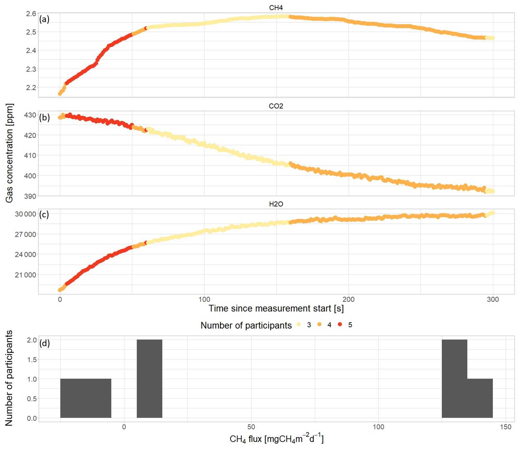
Figure B10 Measurement example (VQC11) of CH₄ concentrations showing an inconsistent trend over the time of the chamber closure. Simultaneous measurements of CH₄ (a), CO₂ (b), and H₂O (c) concentrations over time during chamber closure, with the colors of the data points indicating how many participants included the respective data point in the time period that they chose for flux calculation. Only the responses by participants who gave start and end times for flux calculation were considered for this figure. Histogram of CH₄ fluxes calculated based on the time period chosen by the participants for flux calculation (d).

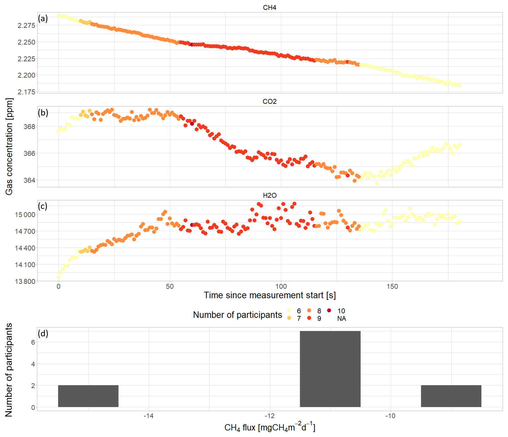
Figure B11 Measurement example (VQC3) of a small linear decrease in CH₄ concentrations over the time of the chamber closure. Simultaneous measurements of CH₄ (a), CO₂ (b), and H₂O (c) concentrations over time during chamber closure, with the colors of the data points indicating how many participants included the respective data point in the time period that they chose for flux calculation. Only the responses by participants who gave start and end times for flux calculation were considered for this figure. Histogram of CH₄ fluxes calculated based on the time period chosen by the participants for flux calculation (d).

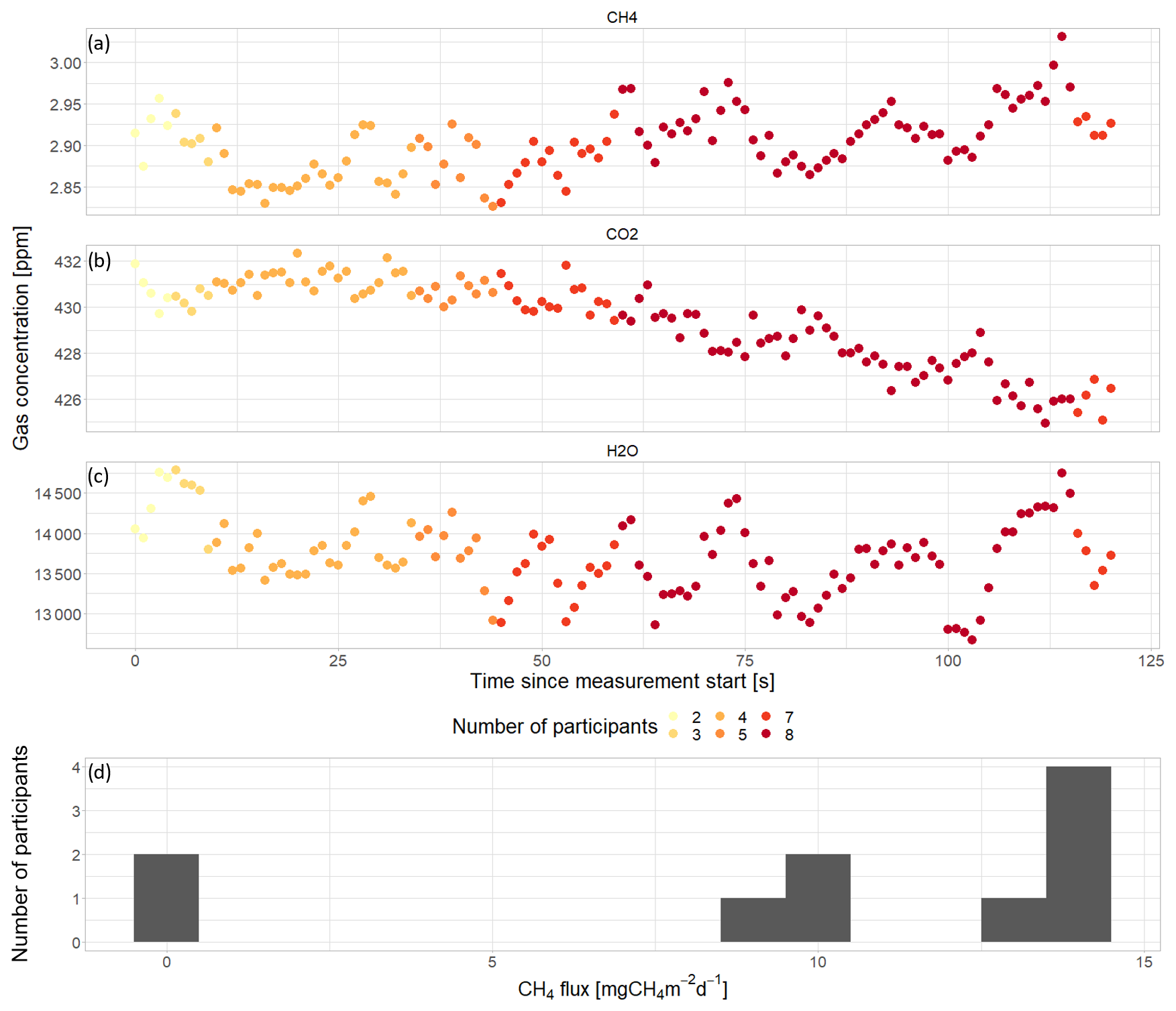
Figure B12 Measurement example (VQC6) with the CH₄ concentrations showing little variation, without a clear trend over the time of the chamber closure. Simultaneous measurements of CH₄ (a), CO₂ (b), and H₂O (c) concentrations over time during chamber closure, with the colors of the data points indicating how many participants included the respective data point in the time period that they chose for flux calculation. Only the responses by participants who gave start and end times for flux calculation were considered for this figure. Histogram of CH₄ fluxes calculated based on the time period chosen by the participants for flux calculation, including the two participants who set the flux to zero (d).

Most participants (66 %) discarded the measurement because they missed a consistent trend of sufficient length in the CH₄ concentrations. Since the changing trend was related to a disturbance or its reason was described as being unclear, the participants did not know which part of the measurement to use for the flux calculation. Additionally, two participants discarded the measurement because they considered the changes in the CH₄ concentration to be too close to zero, and another participant mentioned that the CO₂ and H₂O concentrations did not show a steady trend over time either. Some (23 %) of the participants decided to keep the measurement for flux calculation, all of whom provided start and end times for flux calculation, and one additional participant was uncertain of whether to keep or discard the measurement. The choice of the time periods used for flux calculation depended on the interpretation of the observed pattern in CH₄ concentrations and, thus, strongly influenced the resulting flux estimates. These varied between a CH₄ uptake of −19 mg CH₄ m⁻² d⁻¹ and CH₄ emissions of up to 139 mg CH₄ m⁻² d⁻¹ and appeared as three distinct modes in the flux diagram (Fig. B10d). Two participants chose to keep the entire measurement, resulting in a small positive flux indicating a small net CH₄ emission of 8 to 10 mg CH₄ m⁻² d⁻¹. Three participants decided to use the stronger increase in CH₄ concentrations in the beginning of the measurement, resulting in the highest CH₄ emissions of between 127 and 139 mg CH₄ m⁻² d⁻¹, while two participants assumed that CH₄ was consumed at the plot, using the later decreasing part of the CH₄ concentrations, resulting in negative flux estimates of between −6 and −19 mg CH₄ m⁻² d⁻¹. This resulted in the highest CV among the measurement scenarios, estimated to be 138 %.

B6 Linear decrease

One of the measurements in the visual QC exercise showed a small linear decrease in CH₄ concentrations over time (measurement ID VQC3, Fig. B11). The survey participants largely disagreed on whether this measurement represented a real CH₄ flux. The majority (65 %) of the participants assumed real net CH₄ uptake due to CH₄ oxidation dominating over CH₄ production, while some (19 %) of the participants referred to leakage and too-high initial CH₄ concentrations in the chamber as technical problems causing a false apparent uptake of CH₄. The remaining 15 % of the participants explicitly stated that they were unsure of whether the measurement represented a real flux. A total of 23 % of the participants more specifically mentioned an inconsistent trend in the CH₄ concentrations, referring to three different stages of CH₄ flux or non-linearities at the beginning and at the end of the measurement. As explanations, they referred to initial CH₄ ebullition caused by the chamber placement; changes in the chamber temperature; changes in wind speed combined with chamber leakage; or changes in photosynthetically active radiation (PAR), potentially due to changing cloud cover or due to condensation inside the chamber, as indicated by the simultaneous changes in both CO₂ and CH₄ concentrations as well as by the high H₂O concentrations.

A slim majority (54 %) of the participants discarded the measurement because they did not expect CH₄ uptake in the given environmental (despite the relatively low water table); because of the inconsistent trend in CH₄ concentrations, which makes them unsure of which part of the measurement to use for flux calculation; because of too-high initial concentrations of CH₄ and/or CO₂; or because they suspected anthropogenic disturbance from footprints and compacted vegetation or leakage. The flux estimates derived from the start and end times given by 11 out of the 12 participants who decided to keep the measurement (46 %) differed between the time periods chosen for flux calculation. While five participants chose the entire measurement, resulting in intermediate values of CH₄ uptake, the remaining six participants chose the time period for curve fitting based on the CO₂ concentrations. The middle part of the measurement with linearly decreasing CO₂ concentrations, the beginning of the measurement with stable CO₂ concentrations, and the end of the measurement with linearly increasing CO₂ concentrations were chosen by one, two, and one participant, respectively, while two participants excluded the end of the measurement, resulting in strongly negative, lower negative, stronger negative, and intermediate CH₄ fluxes. Overall, the mean of the flux calculated by the 12 experts keeping this flux was 11.36 mg CH₄ m⁻² d⁻¹, with a CV of 17 %.

B7 No trend

In the visual QC exercise, we included one measurement example for which the CH₄ concentrations did not show a clear trend and varied only a little over the time of the chamber closure (measurement ID VQC6, Fig. B12). Most participants (69 %) noticed the very small change in CH₄ concentrations over the whole measurement, but they disagreed on whether the concentration measurements represented a real flux. Half of them suspected a real emission that remained very small because of CH₄ production and oxidation canceling each other out under conditions of a low water table, and two more participants called it a zero flux, where the uncertainty would likely exceed the flux magnitude. Some (39 %) of the participants, however, explained the low change in CH₄ concentrations with air leakage from the chamber; two of these participants related the leak to vegetation obstructing the chamber seal, and one related the leak to lateral diffusion into the chamber from the surrounding area.

Furthermore, some (19 %) of the participants pointed out an inconsistent trend in the CH₄ concentrations, which they related to a changing balance between CH₄ production and oxidation over time, noisy measurements due to the low precision of the gas analyzer, or a bad chamber seal combined with wind disturbance. According to one participant, the latter was supported by the fluctuations appearing in the concentrations of all three gases, while two other participants mentioned that the CO₂ concentrations looked linear, at least after 30 to 40 s into the measurement, indicating an intact chamber seal.

The majority of the participants (62 %) decided to discard the measurement due to leakage from the chamber (38 %), a changing trend in the CH₄ concentrations (44 %), a too-short measurement time (13 %), or too-high initial concentrations of CH₄ and CO₂ (13 %). While two of these participants manually set the CH₄ flux to zero, one participant pointed out that the concentration changes were too large to be below the precision of the instrument, such that the measurement should not be accepted as a zero flux. Some (31 %) of the participants kept the measurement, assuming a small but nonetheless real CH₄ flux, and gave start and end times for flux calculation. Half of them discarded the beginning of the measurement as a period of initial equilibration, while the other half kept the entire measurement. The choice of different time periods for flux calculation by the participants resulted in a CV of 57 % for this measurement example.