A long-term high-resolution air quality reanalysis with a public-facing air quality dashboard over the Contiguous United States (CONUS)

We present a 14-year, 12 km, hourly air quality dataset (https://doi.org/10.5065/cfya-4g50, Kumar and He, 2023) created by assimilating satellite observations of aerosol optical depth (AOD) and carbon monoxide (CO) in an air quality model to fill gaps in the contiguous United States (CONUS) air quality monitoring network and help air quality managers understand long-term changes in county-level air quality. Specifically, we assimilate the Moderate Resolution Imaging Spectroradiometer (MODIS) AOD and the Measurement of Pollution in the Troposphere (MOPITT) CO observations in the Community Multiscale Air Quality Model (CMAQ) every day from 1 January 2005 to 31 December 2018 to produce this dataset. Meteorological fields simulated with the Weather Research and Forecasting (WRF) model are used to drive CMAQ offline and to generate meteorology-dependent anthropogenic emissions. Both the weather and air quality (surface fine particulate matter (PM_2.5) and ozone) simulations are subjected to a comprehensive evaluation against multi-platform observations to establish the credibility of our dataset and characterize its uncertainties. We show that our dataset captures regional hourly, seasonal, and interannual variability in meteorology very well across the CONUS. The correlation coefficient between the observed and simulated surface ozone and PM_2.5 concentrations for different regions defined by the Environmental Protection Agency (EPA) across the CONUS are 0.77–0.91 and 0.49–0.79, respectively. The mean bias and root-mean-square error for modeled ozone are 3.7–6.8 and 7–9 ppbv, respectively, while the corresponding values for PM_2.5 are −0.9–5.6 and 3.0–8.3 µg m⁻³, respectively. We estimate that the annual CONUS-averaged maximum daily 8 h average (MDA8) ozone and PM_2.5 trends are −0.30 ppb yr⁻¹ and −0.24 µg m⁻³ yr⁻¹, respectively. Wintertime MDA8 ozone shows an increasing but statistically insignificant trend at several sites. We also found a decreasing trend in the 95th percentile of MDA8 ozone but an increasing trend in the 5th percentile. Most of the sites in the Pacific Northwest show an increasing but statistically insignificant trend during summer. An ArcGIS air quality dashboard has been developed to enable easy visualization and interpretation of county-level air quality measures and trends by stakeholders, and a Python-based Streamlit application has been developed to allow the download of the air quality data in simplified text and graphic formats.

1 Introduction

Air quality is one of the most important global environmental concerns, as almost the entire global population (99 %) is estimated to breathe air that exceeds the air quality guidelines defined by the World Health Organization (WHO, 2023). Exposure to ambient air pollution causes about 4.2 million premature mortalities every year (WHO, 2020). Air quality has improved substantially over the past 2 decades in the US, with Environmental Protection Agency (EPA) observations showing that maximum daily 8 h average (MDA8) surface ozone levels have decreased by 29 % over the period from 1980 to 2021, and annual average concentrations of particulate matter with an aerodynamic diameter smaller than 2.5 µm (PM_2.5) have decreased by 37 % over the period from 2000 to 2021 (https://www.epa.gov/air-trends/air-quality-national-summary, last access: 28 April 2025). However, air pollution continues to violate the National Ambient Air Quality Standards (NAAQS) in many parts of the US, such as the Colorado Front Range, California, the northeastern US, and nearly all of the national parks. A recent study reported that 97 % of US national parks suffer from significant or unsatisfactory levels of harm from air pollution (Orozco et al., 2024). Poor air quality is reported to cause about 160 000 premature deaths in the US, with a total economic loss of about USD 175 billion (Im et al., 2018). Exposure to air pollution levels even below the EPA NAAQS can adversely affect human health (Di et al., 2017). To mitigate the risks associated with air pollution and how air quality is responding to emission control policies, it is, therefore, imperative to quantify past changes in air quality.

Numerous studies have revealed several key features of long-term changes in surface ozone and PM_2.5 over the US using long-term observations from the EPA monitoring networks. First, both urban and rural sites in the eastern US show negative ozone trends during the summer season (Butler et al., 2011; Cooper et al., 2012), but lower ozone levels at some sites have an increasing trend during winter and early spring (Bloomer et al., 2010; Cooper et al., 2012; Simon et al., 2015). Second, surface and free-tropospheric ozone show positive trends in all seasons at rural and remote sites in the western US (Jaffe and Ray, 2007; Cooper et al., 2012). Third, increasing ozone is observed in the inflow to the US west coast (Jaffe et al., 2003), over the North Pacific (Parrish et al., 2004), and in the west coast marine boundary layer (Parrish et al., 2009). The Tropospheric Ozone Assessment Report (TOAR) showed that summertime surface ozone continues to decrease over the US, but the trend is less certain at the urban sites (Chang et al., 2017; Fleming et al., 2018). Similar regional and seasonal differences in the long-term trends are also seen in PM_2.5 and its components. For example, carbonaceous aerosols (organic and black carbon) show a widespread decrease over the period from 1990 to 2010 across the US in winter and spring and show positive but insignificant trends over the western US (Hand et al., 2013). PM_2.5 levels continue to decrease over the majority of the US except in the wildfire-prone areas (McClure and Jaffe, 2018).

In addition to the observation-based trend analysis, chemical transport model (CTM) simulations have been employed to interpret the observed trends. For example, the increase in lower ozone values can be attributed to the increase in Asian emissions from 1980 to 1995 (Fiore et al., 2002). The anthropogenic emissions and natural variability were found to have competing effects on surface ozone over much of the US over 1980–2005 (Pozzoli et al., 2011). Another study reproduced negative summertime ozone trends over the eastern US but underestimated the positive trends in the western US, likely due to underestimation of Asian emission trends or trans-Pacific transport or changes in stratosphere–troposphere exchange (Koumoutsaris and Bey, 2012). Lin et al. (2017) quantified the contributions of rising Asian emissions, domestic US emission controls, wildfires, and climate to changes in surface ozone from 1980 to 2014. Several studies have also quantified the contributions of wildfires to PM_2.5 trends in the US (Xie et al., 2020; Burke et al., 2023). While global models captured most of the observed variability and trends in summertime ozone, the use of high-resolution regional models is recommended to reproduce interannual variability in winter and spring in the western US (Strode et al., 2015).

Apart from the interpretation of observed trends, the CTMs also provide information in areas with no observations. However, CTM simulations suffer from both systematic (i.e., biases) and random errors due to a number of factors, including numerical approximations, inadequate understanding of some processes that control the spatial and temporal distribution of air pollutants, inaccuracies in the initialization of the physical and chemical atmospheric state, and uncertainties in the emission inventories. While continuous efforts are being made to improve the representation of processes controlling PM_2.5 and ozone (Appel et al., 2010, 2013, 2017; Nolte et al., 2015; Fahey et al., 2017) and emission inventories are updated by the EPA every 3 years, recent developments have shown that the assimilation of the National Aeronautics and Space Administration (NASA) satellite retrievals of atmospheric composition in CTMs can significantly improve air quality simulations (Gaubert et al., 2016; Kumar et al., 2019; Liu et al., 2011; Pagowski et al., 2014; Saide et al., 2013). NASA satellite retrievals of atmospheric constituents with a far greater spatial coverage compared to ground-based monitoring networks presents a unique opportunity to develop long-term high-resolution air quality reanalysis, which can be useful for quantifying air quality changes in unmonitored areas and assessing the impacts of changes in air quality on human health and ecosystems.

This paper describes the methodology and evaluation of a long-term high-resolution regional air quality reanalysis generated over the CONUS from 2005 to 2018 by assimilating the Moderate Resolution Imaging Spectroradiometer (MODIS) aerosol optical depth (AOD) and the Measurement of Pollution in the Troposphere (MOPITT) carbon monoxide (CO) retrievals daily in the Community Multiscale Air Quality (CMAQ) model. Our regional reanalysis is based on the 3-D variational (3D-Var) approach, which is different from the 4-D variational (4D-Var) approach (Inness et al., 2019) and ensemble Kalman filter (EnKF) approaches (Gaubert et al., 2017; Miyazaki et al., 2020; Kong et al., 2021) used in recent long-term global and regional air quality reanalysis. Among these, 3D-Var is computationally the most efficient approach, as it uses only a single model simulation, but its accuracy can be limited by the assumption of a constant background error covariance matrix that both 4D-Var and EnKF address. An air quality dashboard developed to enable the use of this dataset by a variety of stakeholders is also described.

2 Methodology

2.1 The chemical transport model

The CMAQ model (version 5.3.2) driven offline by the Weather Research and Forecasting (WRF) model (version 4.1) is used to simulate air quality over the CONUS from 1 January 2005 to 31 December 2018. We employ the “cb6r3_ae7_aq” chemical mechanism that uses Carbon Bond 6 version r3 for gas-phase chemistry and the AERO7 aerosol module for representing aerosol processes, including secondary organic aerosols (Appel et al., 2021). Both the WRF and CMAQ models use a horizontal grid spacing of 12 × 12 km², with the WRF (CMAQ) grid using 481 (442), 369 (265), and 36 (35) grid points in the longitudinal, latitudinal, and vertical directions, respectively. The model top is set to 50 hPa for both the models. The meteorological initial and boundary conditions for WRF are based on the 6-hourly ERA-Interim analyses at a grid spacing of 0.7° × 0.7°. We follow Appel et al. (2017) for physical parameterizations, 4-D data assimilation, and soil moisture nudging settings in WRF.

Emissions from several anthropogenic emissions sectors, such as residential wood combustion, agricultural emissions from livestock and fertilizer applications, and mobile sources, depend on meteorological conditions. For example, ambient temperature affects the heating demand, impacts the volatilization of emissions from fertilizer use, drives air-conditioning use, etc. The Sparse Matrix Operator Kernel Emissions (SMOKE) modeling system allows us to simulate these relationships. To be consistent in the use of meteorological fields for both emission processing and driving CMAQ, we generate meteorology-dependent anthropogenic emissions for the EPA National Emissions Inventory (NEI) base years of 2011, 2014, and 2017 by feeding the WRF meteorological fields to SMOKE. The emissions for 2005–2010 are derived by applying EPA-reported annual state-wise trends to the NEIv2 2011 emissions. While NEI emissions are available for 2005 and 2008, the emission processing platform for 2005 and 2008 does not process emissions for the “cb6r3_ae7_aq” chemical mechanism of CMAQ used here. Similarly, NEIv2 2014 emissions are used to derive emissions for 2012 and 2013, and the NEIv1 2017 emissions are used to derive anthropogenic emissions for the rest of the years. Fire emissions in CMAQ are represented using the Fire Inventory from NCAR (FINN; version 2.2), which provides daily varying global fire emissions at a 1 × 1 km² resolution (Wiedinmyer et al., 2023). FINN emissions are processed through SMOKE to enable the inline plume rise of fire emissions within CMAQ. Biogenic emissions are calculated online within the model using the Biogenic Emission Inventory System (BEIS). The chemical boundary conditions are based on 6-hourly Whole Atmosphere Community Climate Model (WACCM) simulations (Marsh et al., 2013; Gettelman et al., 2019). The WACCM output is mapped onto CMAQ grids using the Initial Conditions Processor (ICON) and Boundary Conditions Processor (BCON).

2.2 Data assimilation system

We have used the 3-D variational (3D-Var) capability of the community Gridpoint Statistical Interpolation (GSI) system (version 3.5) to assimilate the Level-2 MODIS AOD retrievals and the Level-2 MOPITT CO retrievals in CMAQ. The MODIS AOD assimilation framework is the same as we developed previously (Kumar et al., 2019), and the MOPITT CO assimilation capability has been developed in this work. We use total aerosol mass per mode (Aitken, accumulation, and coarse) and CO mixing ratios as the control variables in GSI. The state variables include individual aerosol components, total aerosol mass per mode, CO mixing ratios, meteorological variables (temperature, pressure, and relative humidity), and the CMAQ vertical grid. Daily MODIS and MOPITT retrievals are converted into a format compatible with GSI input modules.

A climatological background error covariance (BEC) matrix is generated separately for winter (January) and summer (July) conditions using the GEN_BE tool, which reads two different WRF-CMAQ runs driven by different meteorological and emission inputs but valid at the satellite overpass time. As there are multiple overpasses of the Terra and Aqua satellites that host the MOPITT and MODIS sensors, we calculate the BEC at 15:00, 18:00, and 21:00Z. The winter BEC is used when assimilating satellite retrievals from November through March, whereas the summer BEC is used for the rest of the months. Our BEC design considers the uncertainties in meteorology, anthropogenic emissions, and biomass burning emissions. Meteorological uncertainties are represented by using two different sets of physical parameterizations (Table A1) in two WRF runs to capture errors in meteorology related to assumptions used in physical parameterizations. Species-dependent perturbation factors for anthropogenic and biomass burning emissions are estimated by comparing a number of available global/regional anthropogenic and biomass burning emission inventories over the CONUS (Tables A2 and A3.3). Among the two WRF-CMAQ runs fed to GEN_BE for BEC estimation, we used the default emissions in the first run and perturbed the emissions in the second run. The BEC was then estimated in terms of variances and length scales (both horizontal and vertical) for total aerosol mass per mode and CO, and it was used in GSI. We refer the reader to Kumar et al. (2019) for a description of BEC parameters.

We have assimilated standard Level-2 Collection 6.1 MODIS AOD and version 8 MOPITT CO retrievals based on the multispectral (thermal and near-infrared) algorithm in CMAQ. This multispectral product is more sensitive to near-surface CO over land compared to the thermal-infrared-only retrievals. MOPITT retrievals agree with in situ measurements within ±5 % at all vertical levels (Deeter et al., 2019). The observation errors for MODIS AOD retrievals are specified as (0.03 + 0.05 ⋅ AOD) and (0.05 + 0.15 ⋅ AOD) over the ocean and the land, respectively (Remer et al., 2005). The observation errors for CO profiles are used as reported in the MOPITT retrieval product. A simple forward operator and its adjoint based on the parameterization of Malm and Hand (2007) is used to convert the CMAQ aerosol chemical composition into AOD for a direct comparison with MODIS AOD retrievals as described in Kumar et al. (2019). The forward operator and its adjoint for MOPITT CO assimilation are developed in this study and described in Appendix A1.

2.3 Reanalysis production workflow

Daily analyses of 3-D fields of aerosols and CO based on the assimilation of MODIS AOD and MOPITT CO retrievals in CMAQ using the GSI system has been performed using the workflow shown in Fig. 1. The first CMAQ simulation on 1 January 2005 is initialized using the global model simulations from WACCM, and all subsequent simulations until 31 December 2018 are initialized from the previous CMAQ simulations. Every day, we perform nine simulations following the availability of new satellite observations every 3 h owing to difference between Terra and Aqua overpass times. The first simulation runs CMAQ from 00:00 to 15:00Z, the second simulation assimilates MODIS Terra and Aqua AOD retrievals at 15:00Z, and the third simulation assimilates MOPITT CO retrievals at 15:00Z. The fourth simulation advances CMAQ from 15:00 to 18:00Z, with the fifth and sixth simulations assimilating MODIS AOD and MOPITT CO at 18:00Z, respectively. The seventh simulation advances CMAQ from 18:00 to 21:00Z, the eighth simulation assimilates MODIS Aqua AOD retrievals at 21:00Z, and the ninth simulation advances CMAQ from 21:00 to 00:00Z of the next day. This resulted in a total of 46 152 jobs being submitted to the NCAR Cheyenne supercomputer (https://arc.ucar.edu/knowledge_base/70549542, last access: 28 April 2025). An automated script was developed to submit and track successful completion of these jobs.

Figure 1 Architecture of the daily CMAQ- and GSI-based chemical data assimilation workflow.

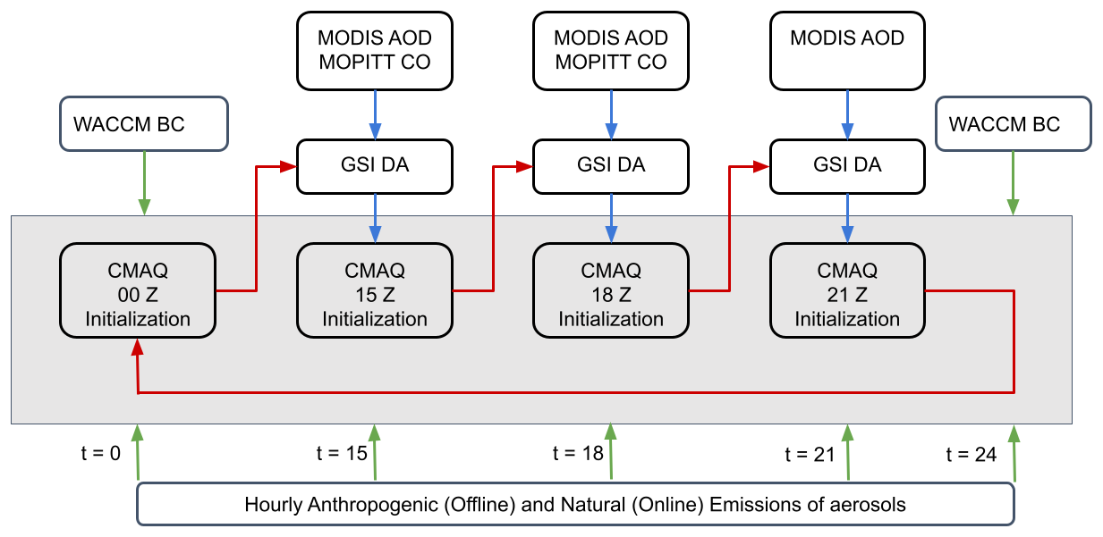
The assimilation times of 15:00, 18:00, and 21:00Z were determined based on the analysis of overpass times of Terra and Aqua satellites, which pass over the CONUS between 13:30 and 22:30Z. All of the satellite retrievals belonging to a 3 h window are assumed to be available for assimilation at the center of that window. For example, all of the satellite retrievals between 13:30 and 16:30Z are assimilated at 15:00Z.

Our previous work has shown that the assimilation of MODIS AOD in CMAQ improved the correlation coefficient between CMAQ-simulated and independently observed PM_2.5 by ∼ 67 % and reduced the mean bias by ∼ 38 % over the CONUS during July 2014. To understand whether GSI pushes CMAQ towards MOPITT, we performed and compared 1 month (July 2018) of CMAQ experiments with and without assimilation of MOPITT CO profiles. We find that the assimilation of MOPITT CO profiles substantially improves the correlation coefficient and reduces the errors (both mean bias and root-mean-square error) between CMAQ and MOPITT CO at all of the pressure levels except at 100 hPa, where the MOPITT sensitivity is the lowest (Appendix A2, Fig. A1). This simple test confirms the ability of GSI to constrain the performance of CMAQ with satellite observations. Other trace gas species (e.g., ozone and OH) are not affected directly by the assimilation of AOD and CO, but the impact of assimilation indirectly affects these species through photochemical processes in the model. For example, we found instantaneous changes in surface ozone in the range of −1.3 to 3.2 ppbv, but monthly average changes are within the range of ±0.3 ppbv during July 2018.

2.4 Output frequency and optimization

The production of a chemical reanalysis also poses the challenge of storing the model output. As our chemical reanalysis focuses on air quality applications, we saved all of the chemical variables together with relevant meteorological parameters (2 m temperature and relative humidity, 10 m wind speed and direction, planetary boundary layer height, precipitation, and downward-reaching solar radiation) and deposition (both dry and wet) fluxes every hour at the surface. The total size of this output is 12 TB.

3 Ground-based observations and the trend calculation method

We have obtained and processed hourly in situ measurements of 2 m temperature (T2), 2 m relative humidity (RH), 10 m wind speed (WS10), 10 m wind direction (WD10), and surface pressure from the METeorological Aerodrome Reports (METAR) network, which is distributed by the National Centers for Environmental Prediction's Meteorological Assimilation Data Ingest System (MADIS). METAR data are surface weather observations and consist of meteorological data from airports (Automated Surface Observing Systems) and other permanent weather stations (Automated Weather Observing Systems) located throughout the US. We used the Level-3 quality-controlled METAR data over the CONUS to evaluate our modeled meteorological fields (https://doi.org/10.5065/cfya-4g50, Kumar and He, 2023). Daily precipitation data from the 0.1° Integrated Multi-satellitE Retrievals for Global precipitation measurements (IMERG; https://gpm.nasa.gov/data/imerg, last access: 28 April 2025) dataset is used to evaluate WRF-simulated precipitation.

To evaluate the modeled surface PM_2.5 and ozone concentrations, we have obtained hourly PM_2.5 and ozone observations from the EPA Air Quality System (AQS), which currently measures PM_2.5 and ozone at more than 1000 sites across the US. The AQS data also contain values below the method detection limit (MDL). The MDLs are different for ozone and PM_2.5 and also vary as a function of site and instrument type. For consistency, we assume MDL values of 5 ppb for ozone and 2 µg m⁻³ for PM_2.5 for all sites. All of the data below the MDL were replaced by MDL/2 (https://www3.epa.gov/ttnamti1/files/ambient/airtox/workbook/AirtoxWkbk4Preparingdataforanalysis.pdf, last access: 28 April 2025; https://pubs.acs.org/doi/10.1021/es071301c, last access: 28 April 2025). At sites for which two simultaneous measurements (corresponding to two instruments) were available, the mean value was taken for further calculation.

The trend calculations were performed using both the observed and modeled ozone and PM_2.5 values. The monthly mean time series of observed and modeled maximum daily 8 h (MDA8) ozone and 24 h average PM_2.5 during 2005–2018 is calculated over all measurement sites. The daily MDA8 ozone over a site is calculated using the EPA's defined methodology (https://www.govinfo.gov/content/pkg/FR-2015-10-26/pdf/2015-26594.pdf, last access: 28 April 2025, 168 pp.). For each day, 8 h running averages are taken from 07:00 to 23:00 LST (local standard time), which constitutes 17 valid 8 h running mean values per day. If an 8 h window has less than 6 h of data and the mean value of the remaining hours is less than 70 ppb, the data for that window are discarded. If a site has fewer than 13 valid 8 h mean values or the maximum value of the available 8 h average is less than 70 ppb, the value for that day is discarded. For PM_2.5, a daily 24 h average value is calculated in local standard time only if at least 18 h of valid data per day are available. Furthermore, we discarded (1) all sites with < 50 % data per month, (2) all sites with < 50 % data during each year, and (3) all sites for which the number of years with ≥ 50 % data was < 10 during 2005–2018. The number of valid sites fulfilling the above criteria over the CONUS is estimated to be 1012 and 369 for MDA8 ozone and 24 h PM_2.5, respectively. Daily values of MDA8 ozone and 24 h PM_2.5 are used to calculate the monthly 5th percentile, 50th percentile, 95th percentile, and mean time series during 2005–2018 at each valid site. A similar criterion for the seasonal mean and for the 5th, 50th, and 95th percentile time series was also used. The number of valid sites reached a maximum (1010 and 357 for MDA8 O₃ and 24 h PM_2.5, respectively) during summer season, whereas it reached a minimum (501 and 337 for MDA8 O₃ and 24 h PM_2.5, respectively) during the winter season. These annual and seasonal MDA8 ozone and PM_2.5 time series are then used to estimate annual and seasonal trends, and the significance of trend values are also tested.

4 Results and discussion

4.1 Meteorological evaluation

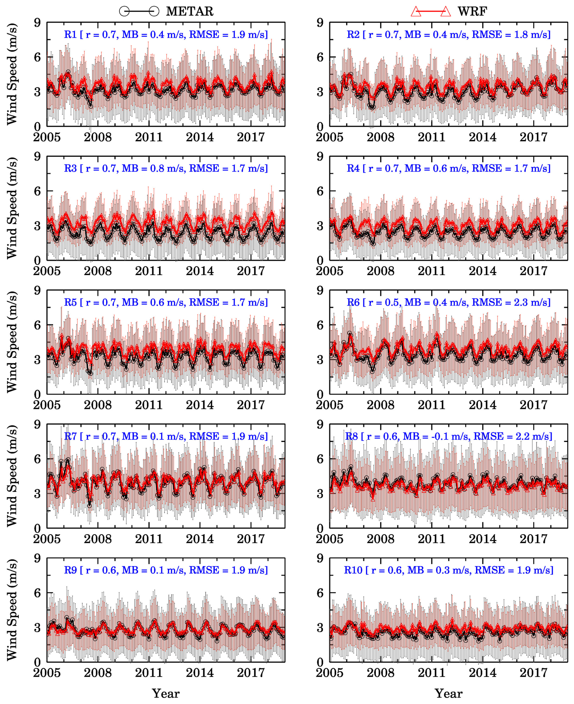
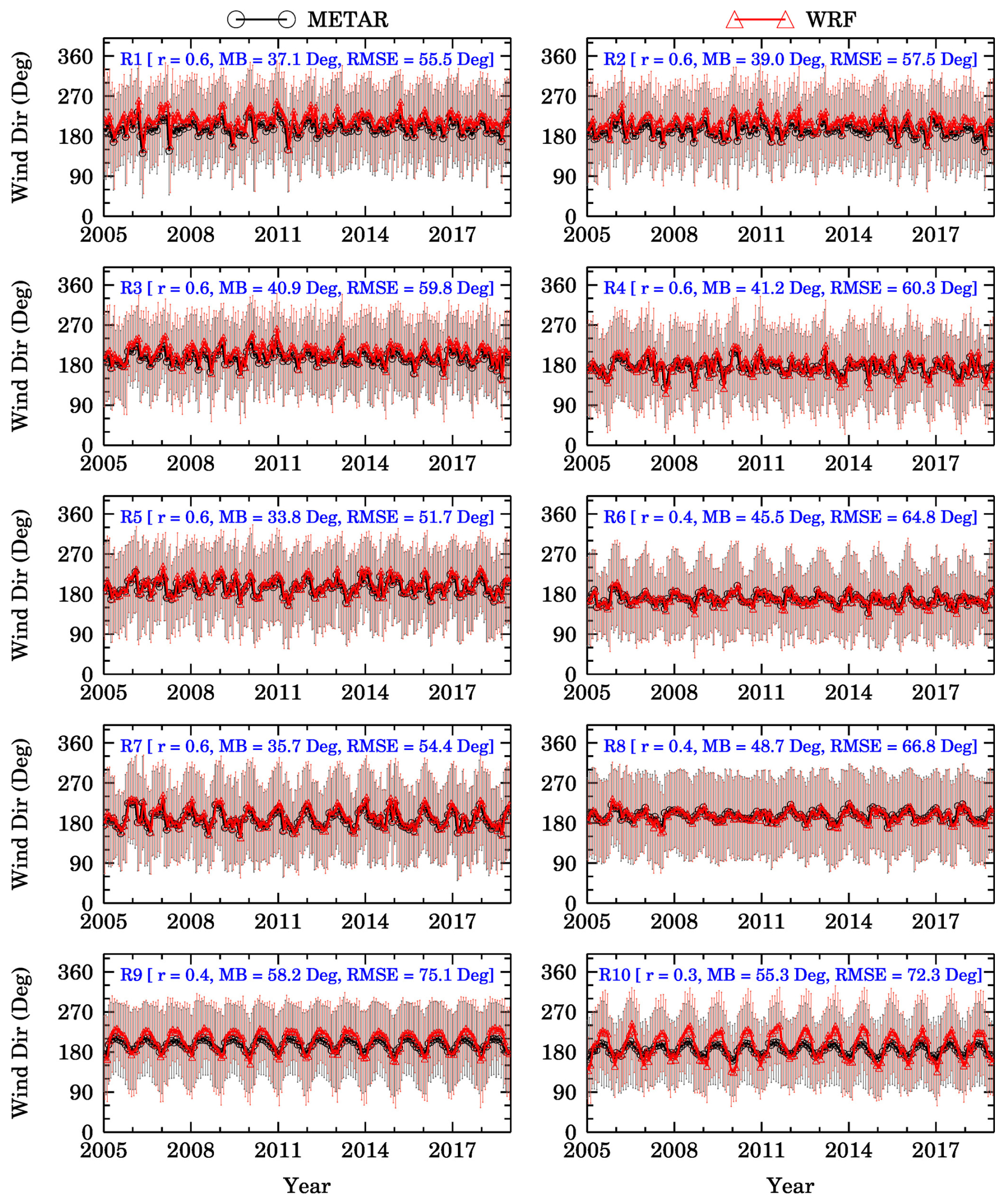
The WRF simulations for the entire period (2005–2018) processed using the Meteorology–Chemistry Interface Processor (MCIP) are co-located with METAR observations of T2, RH, WS10, and WD10 in space and time, and paired values are used for evaluating the model. The evaluation is performed at a regional scale, following the EPA regional classification of the CONUS, in 10 regions (see Appendix A2, Fig. A2). The number of METAR sites during 2005–2018 was 1290, and the maximum percentage of available hourly data during the study period was 33 %–68 % over 10 EPA regions. Region 8 has the fewest data (∼ 33 %–37%), and other regions have 47 %–68 % data during 2005–2018. Monthly regionally averaged model and METAR observations time series are compared over 10 EPA regions for T2 (Fig. 2), RH (Fig. 3), WS10 (Fig. 4), and WD10 (Fig. 5). Three statistical metrics, namely, the correlation coefficient (r), mean bias (MB), and root-mean-square error (RMSE), for each region are also listed in Figs. 2–5.

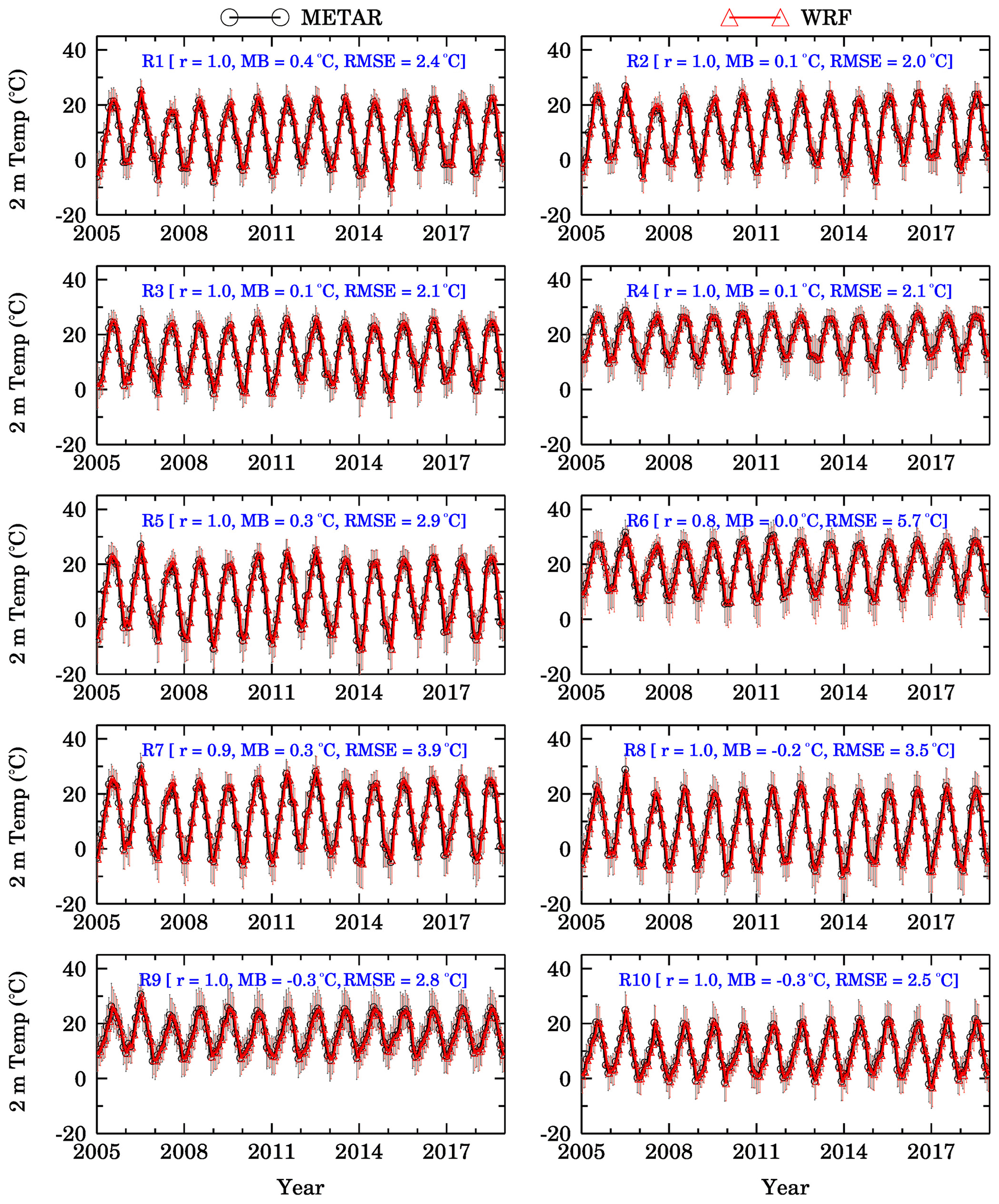
Figure 2 Time series of monthly averaged 2 m temperature over 10 EPA regions (R1–R10) from the WRF-CMAQ setup (red) and METAR observations (black) during 2005–2018. Orange and gray lines represent the standard deviation for WRF-CMAQ and METAR, respectively. The correlation coefficient (r), mean bias (MB), and root-mean-square error (RMSE) for each region are also shown.

Figure 3 Same as Fig. 2 but for 2 m relative humidity (RH).

Figure 4 Same as Fig. 2 but for 10 m wind speed.

Figure 5 Same as Fig. 2 but for 10 m wind direction.

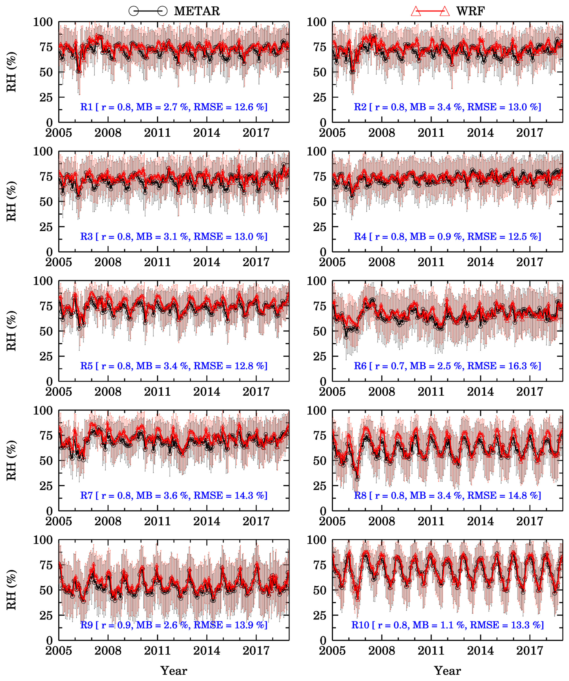
Monthly regionally averaged T2 between the model and observations (Fig. 2) shows excellent correlations of 0.8–1.0, low mean biases of −0.3 to 0.4 °C, and an RMSE ranging from 2.0 to 5.7 °C over the 10 EPA regions. The model also performed well (r= 0.7–0.9) with respect to simulating RH (Fig. 3) over 10 EPA regions, with mean biases of 0.9 %–3.6 % and an RMSE of 12.5 %–16.3 %. As RH is estimated as a ratio of vapor pressure to saturation pressure (es) and es depends on T2, the biases in T2 also contribute to the biases in RH. For example, EPA Region 6 shows the highest T2 RMSE and the highest RH RMSE. The model reproduces the variations in surface pressure very well (r= 1.0) with a slight underestimation (MB = −8.1 to 0.2 hPa; RMSE = 0.3–8.1 hPa). The slight underestimation in pressure is seen in 8 out of 10 EPA regions, with the largest MB in regions 9 (−8.1 hPa) and 10 (−7.4 hPa). The errors in surface pressure (plot not shown) over these regions could also contribute to biases in T2 and RH.

Prior to the 10 m wind speed comparison, model wind speeds are assigned a “zero value” if the hourly wind speed at any site is less than 0.51 m s⁻¹ (1 knot). This step was needed to make the model output consistent with the METAR wind speed data, which treats such wind speeds as calm winds and assigns them a zero value. Our model simulation slightly overestimates (MB = 0.1–0.8 m s⁻¹) WS10 (Fig. 4) over most of EPA regions with the exception of Region 8 (MB = −0.1 m s⁻¹). Wind direction (Fig. 5) biases (absolute) over these regions were 34–58°. The correlation coefficients for both WS10 and WD10 are slightly lower in regions 8–10, likely due to the complex topography in these regions. The correlation coefficients for the 10 m wind speed were lower than those for temperature and relative humidity, indicating a slightly poorer model performance for winds. The WRF model is known to overpredict the 10 m wind speed at low to moderate wind speeds in all available planetary boundary layer (PBL) schemes (Mass and Ovens, 2010). This shortcoming of the model has been partly attributed to unresolved topographical features by the default surface drag parameterization, which in turn influences surface drag and friction velocity, and partly to the use of coarse horizontal and vertical resolutions of the domain (Cheng and Steenburgh, 2005). The WRF model also captures the seasonally averaged diurnal variations in T2, RH, and 10 m wind speed very well, but it overestimates the wind speed, particularly at night (see Appendix A2, Fig. A3).

As WRF and IMERG precipitation have different resolutions, we first mapped the WRF-simulated precipitation from a 12 km × 12 km grid on a Lambert conformal projection to the IMERG rectilinear grid of 0.1° × 0.1° using the “rcm2rgrid” functionality of the NCAR command language (https://www.ncl.ucar.edu/Document/Functions/Built-in/rcm2rgrid.shtml, last access: 28 April 2025). The seasonal mean WRF-simulated and IMERG-derived precipitation values are then compared over four seasons during 2005–2018 (Fig. 6). The model is able to capture the spatial patterns in precipitation in different seasons, with an underestimation of −0.1 to −0.9 mm d⁻¹. The highest underestimation is observed during the winter season. The eastern CONUS showed an underestimation during the winter, spring, and autumn seasons; however, over the western US, the model mostly overestimated the precipitation, especially in the mountainous regions (Rockies, Cascades, and Sierra Nevada). The model also showed larger biases over the lakes and oceanic regions. Despite the biases, this comprehensive evaluation shows that our model simulations captured the key features of the regional and temporal variability in the key meteorological parameters over the CONUS fairly well.

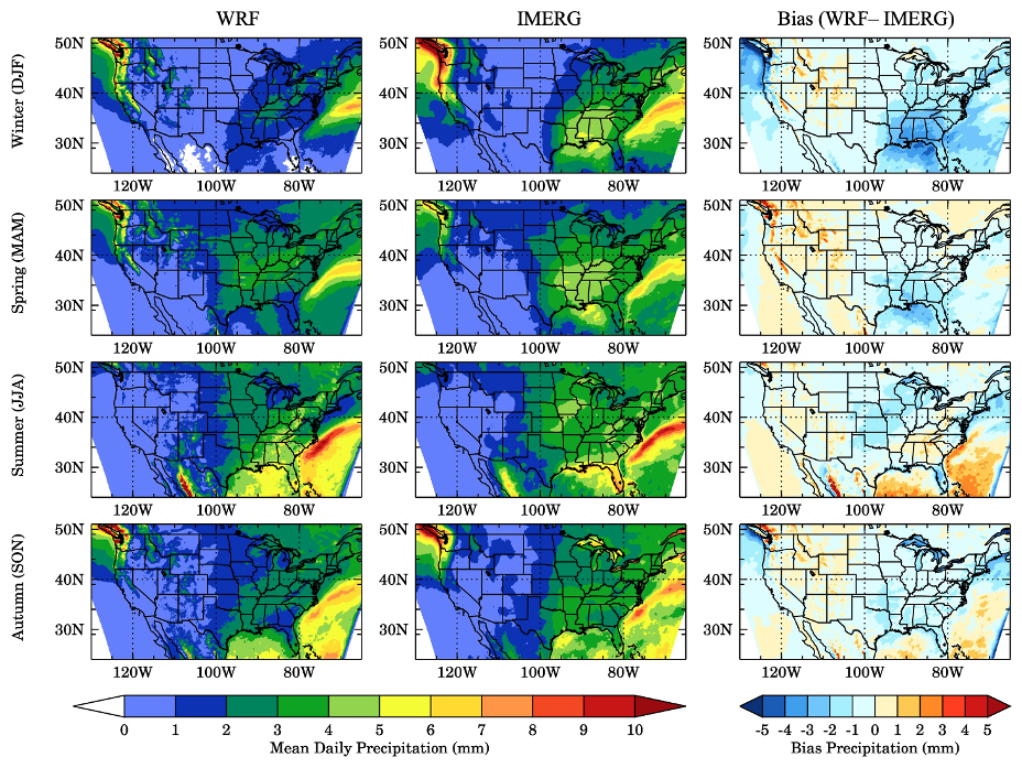
Figure 6 Spatial distribution of mean daily precipitation and bias during four seasons in 2005–2018 (top to bottom: winter, spring, summer, and autumn). The left-hand, center, and right-hand columns represent mean precipitation from WRF, mean precipitation from IMERG, and the precipitation bias (WRF − IMERG), respectively.

4.2 Air quality evaluation

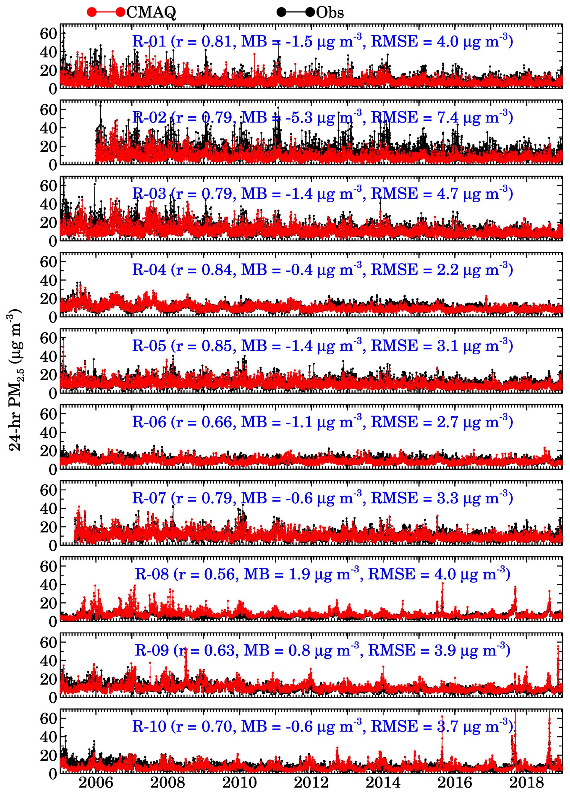
Hourly regionally averaged observed and CMAQ-simulated surface ozone and PM_2.5 are compared for all of the EPA regions in Figs. 7 and 8, respectively. In all of the regions, the model captures the seasonal cycle in surface ozone, characterized by a summertime peak, and the observed interannual variability very well, with correlation coefficients of 0.77–0.91. The model also overestimates the nighttime ozone levels in all of the regions (see Appendix A2, Fig. A4), but a larger overestimation is seen in regions 8 and 9. The mean bias and RMSE in modeled ozone are very similar across the regions, with values ranging from 3.7 to 6.8 and from 7.0 to 9.0 ppbv, respectively. The model shows a slightly poorer skill with respect to capturing the variability in PM_2.5 relative to ozone, as reflected by smaller r values of 0.49–0.79, but it captures long-term trends in most of the regions reasonably well. The mean bias and RMSE in modeled PM_2.5 are estimated to be −0.9 to 5.6 and 3.0 to 8.3 µg m⁻³, respectively. The largest underestimation of PM_2.5 is seen in Region 8, particularly from 2005 to 2012, while the largest overestimation is seen in Region 2.

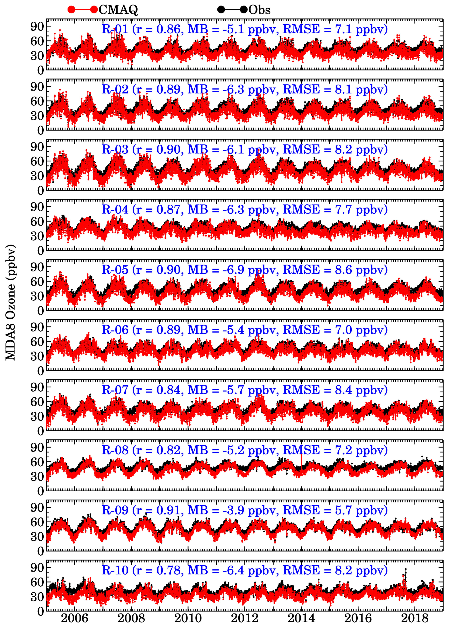
Figure 7 Time series of hourly averaged surface ozone over 10 EPA regions (R1–R10) from the WRF-CMAQ setup (red) and EPA AQS observations (black) during 2005–2018. The correlation coefficient (r), mean bias (MB), and root-mean-square error (RMSE) for each region are also shown.

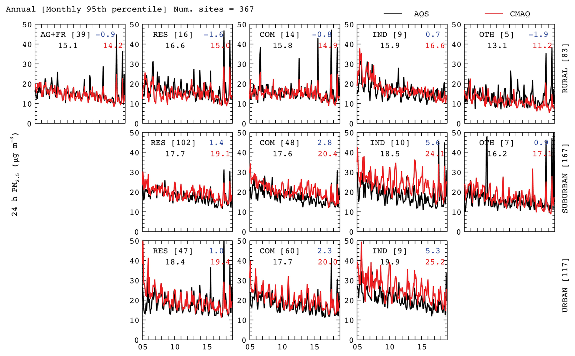
In addition to the regional evaluation, we also evaluated the model performance for different land use types and location settings (see Fig. A5 in Appendix A2 for a classification of the number of sites in these categories). This categorization information by land use and location type was not available for a very small number of sites; thus, these sites were excluded from the analysis (sites classified as “NONE” in Fig. A2). As maximum daily averaged 8 h (MDA8) ozone and daily averaged PM_2.5 are policy-relevant metrics, we focus on the evaluation of these parameters on a monthly averaged scale for this evaluation. We evaluate the monthly median (50th percentile) and the 5th and 95th percentile time series of MDA8 ozone and daily averaged PM_2.5 for different land use categories and location settings (Appendix A2, Figs. A2.6–A2.11).

Among the rural sites, all land use categories showed the highest biases for the 5th percentile, followed by the median and 95th percentile for MDA8 ozone, except for the “Others” category, for which the median showed the lowest bias. For suburban and urban site types, the 95th percentile MDA8 ozone consistently showed the lowest bias for all land use types, followed by the median and 5th percentile. Furthermore, the Others land use category at rural and urban sites shows the lowest bias for the 5th percentile and the median, whereas the “Residential” land use type shows the lowest bias for the suburban sites.

Figure 8 Same as Fig. 7 but for daily averaged surface fine particulate matter (PM_2.5).

For PM_2.5, the largest differences between the model and observations are seen for the 95th percentile for the Others land use category compared to the 5th percentile and median. The model generally captures the temporal variability in PM_2.5 across all land use types (except Others) and location settings for all three percentile metrics analyzed here, although some anomalies are also evident. For example, residential and commercial sites in the urban category show a larger overestimation for the median and 95th percentiles during 2005–2006, indicating higher uncertainties in anthropogenic emission estimates at these sites during these years. While the model follows most of the observed peaks in 95th percentile, it substantially underestimates the observed peaks.

The errors in air quality simulations can be attributed to the uncertainties in the different types of emissions used to drive air quality models, errors in the lateral boundary conditions representing pollution inflow, uncertainties in meteorological parameters (as quantified earlier in this section), and the poor understanding of some of the physical and chemical processes controlling the fate of those emissions. To quantify uncertainties in anthropogenic and biomass burning emissions over the CONUS, we compared all available anthropogenic and biomass burning emission inventories over the region and found that anthropogenic emission estimates across various emission inventories vary by a factor of 1.16–2.94 (Table A2) and the corresponding fire emission estimates vary by factor of 3.13–8.0 (Table A3). The extrapolation of the NEI emissions to years other than the base years might have also introduced some uncertainties in our simulations, as EPA-reported state-level trends may not always represent local (sub-state) changes in emissions and also do not provide information about new emission sources appearing in the CONUS between two NEI base emission inventory years. In addition, the observation error (0.05 + 15 % of MODIS AOD value over land; Remer et al., 2005) for MODIS AOD increases with increases in the magnitude of the AOD which, in turn, restricts the data assimilation system (GSI) in pushing the modeled AOD towards the MODIS AOD. Furthermore, the AOD retrievals do not contain any information about the vertical distribution of aerosols; thus, GSI simply scales the modeled vertical profile to match the MODIS AOD within the constraints of observation and model error. Therefore, AOD assimilation is unable to correct for any errors in the vertical distribution of aerosols resulting from errors in the plume rise of fire emissions.

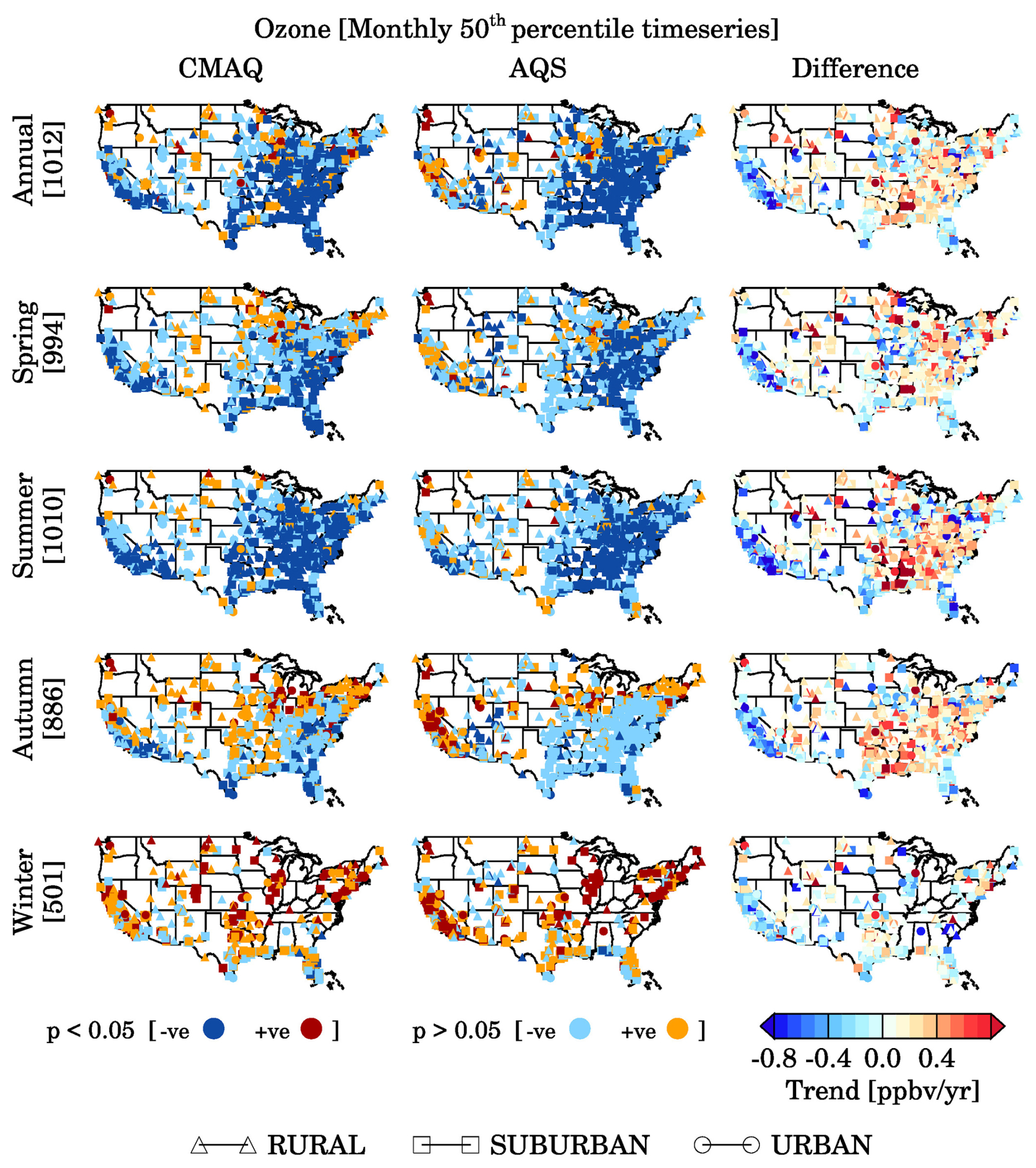
Figure 9 Spatial distribution of positive (blue colors) and negative (red colors) trends in MDA8 ozone at different levels of statistical significance (p values) using annual and seasonal monthly median time series (top to bottom). Plots on the right show the differences in trend values (CMAQ − AQS).

4.3 Trend analysis

To help air quality managers and the public determine the confidence that they can put in using this reanalysis for analyzing changes in air quality in their regions, we have evaluated the trends in our CMAQ-simulated MDA8 ozone and 24 h average PM_2.5 against the AQS observations. The spatial distribution of positive/negative trend values in MDA8 ozone and 24 h average PM_2.5 calculated using monthly median values in AQS and CMAQ data during 2005–2018 are shown in Figs. 9 and 10, respectively. Different symbols are used to represent urban, suburban, and rural site types. Based on location, ∼ 42 % and 23 % of sites were in rural areas, ∼ 41 % and 45 % of sites were in suburban areas, and ∼ 17 % and 32 % of sites were in urban or city centers for MDA8 ozone and 24 h average PM_2.5, respectively. Darker (lighter) red and blue colors represent statistically significant (insignificant) increasing and decreasing trends at the 2σ level. The 2σ rule is a standard way of testing the statistical significance of trends. In a normal distribution, ∼ 95 % of the data points lie within 2 standard deviations (±2σ) of the mean. If the trend falls outside this range, it is considered unlikely to have occurred by chance (i.e., at a statistical significance in the probability of less than 5 %). Over the study period, both the model and observations show decreasing trends in MDA8 ozone over the majority of the CONUS. Most sites in the eastern US show decreasing trends that were statistically significant, with p values than 0.05. The sites located in the western or northwestern US, however, showed mixed results, with some sites showing increasing trends, most of which were not statistically significant. Similar results were observed during the summer season, with most sites showing statistically significant decreasing trends over most locations. During the autumn and winter seasons, several sites over California and the eastern US showed decreasing but insignificant trends. Some sites over the midwestern US also changed their trend sign during these seasons. The trends in the winter seasons were mostly positive over most sites in the US (except for the coastal sites in the southeastern US). About 55 % (278 of 501) of the sites showed positive trends in both AQS and CMAQ data during winter, but only ∼ 3 % (29 of 1012) of the sites showed positive trends in summer. The seasonal changes in monthly median trends discussed above were mostly consistent (67 %–86 %) between the AQS and CMAQ data. A similar analysis with the 5th and 95th percentile time series suggested that the higher percentiles showed mostly decreasing trends, but the 5th percentile dataset for the Midwestern US, Boston–New York–DC, and central US sites showed increasing trends on a seasonal and annual basis. The MDA8 ozone trend over the CONUS (1012 sites) is estimated to be −0.53 ± 0.46 and −0.56 ± 0.45 ppb yr⁻¹ (using summertime data) and −0.31 ± 0.43 and −0.29 ± 0.39 ppb yr⁻¹ (using data from all seasons) for AQS and CMAQ data, respectively, with most sites (∼ 70 %) showing negative trends. At the 2σ level (p value < 0.05), the summertime mean ozone trends are −0.85 ± 0.36 and −0.75 ± 0.35 ppb yr⁻¹ for 484 and 620 respective sites, whereas annual MDA8 ozone trends are −0.52 ± 0.45 and −0.47 ± 0.42 ppb yr⁻¹ for 554 and 562 respective sites for AQS and CMAQ data, respectively, over the CONUS. This suggests decreases in monthly high-ozone days but increases in monthly low-ozone days. On an annual basis, MDA8 ozone showed the most decreasing trends (AQS and CMAQ = −0.40 ± 0.37 and −0.34 ± 0.34 ppb yr⁻¹, respectively) at the 428 rural sites. The mean ozone trends over urban (411 sites) and suburban (170) areas were −0.28 ± 0.44 (AQS) and −0.29 ± 0.40 ppb yr⁻¹ (CMAQ) and −0.13 ± 0.48 (AQS) and −0.15 ± 0.48 ppb yr⁻¹ (CMAQ), respectively. The ozone trends over high-altitude sites (16 sites) are mostly negative in summer (AQS and CMAQ = −0.43 ± 0.45 and −0.12 ± 0.36 ppb yr⁻¹, respectively) and on an annual basis (AQS and CMAQ, = −0.39 ± 0.38 and −0.03 ± 0.29 ppb yr⁻¹, respectively).

Similar MDA8 ozone trends were also reported in a previous study (Simon et al., 2015). Mousavinezhad et al. (2023) reported that all regions except the Northern Rockies and the southwestern US experienced decreasing trends in median MDA8 ozone values during the warm season of 1991–2020, with rural stations in the southwestern US and urban stations in the northeastern US experiencing the greatest declines of −1.29 ± 0.07 and −0.85 ± 0.08 ppb yr⁻¹, respectively. They also reported a large decrease in the MDA8 ozone 95th percentile in all regions. Similarities in ozone trends between the AQS observations and CMAQ simulations over a longer time period (1990–2015) have also been reported by He et al. (2020).

On an annual basis, the 24 h average PM_2.5 also showed mostly decreasing trends (∼ 79 %) over most of the sites. A majority of these trends were also statistically significant at the 2σ level (AQS and CMAQ = 70 % and 75 %, respectively). However, unlike MDA8 ozone, an increasing trend (although insignificant) in summertime PM_2.5 is observed over the northwestern US (Fig. 10). The wintertime trends were also mostly decreasing over most of the sites, except for the northwestern US. During the summer season an approximate 5-fold increase (annual ∼ 5 %; summer ∼ 24 %) in positive trends is observed in high-PM_2.5 days (95th percentile time series), with most of these increases observed over the Pacific Northwest. These summertime increases in PM_2.5 trends are also evident from the 95th percentile time series, where a sharp increase in PM_2.5 is observed during 2017–2018 over all sites except industrial locations (see Fig. A11). In recent years, these changes could be even stronger, as wildfire activity over the western US has increased in the last decade. Dramatic decreasing trends in PM_2.5 in the eastern US have also been reported in previous studies (Zhang et al., 2018; Gan et al., 2015; Xing et al., 2015) (Gan et al., 2015; Xing et al., 2015; Zhang et al., 2018) due to emission reductions. The increasing trend in the western central area of the US is due, in part, to frequent wildfires (Dennison et al., 2014; McClure and Jaffe, 2018). For PM_2.5, the overall mean trends are −0.24 ± 0.21 and −0.24 ± 0.24 µg m⁻³ yr⁻¹ (369 sites) in the AQS and CMAQ datasets, respectively. Unlike MDA8 ozone, the number of sites remained almost the same (337–357 sites in the four seasons and 369 on an annual basis) during seasons, and an overall negative trend is also observed (−0.18 ± 0.25 to −0.30 ± 0.35 µg m⁻³ yr⁻¹). At the 2σ level, the number of sites that showed negative trends in both the datasets was 69 %–80 %.

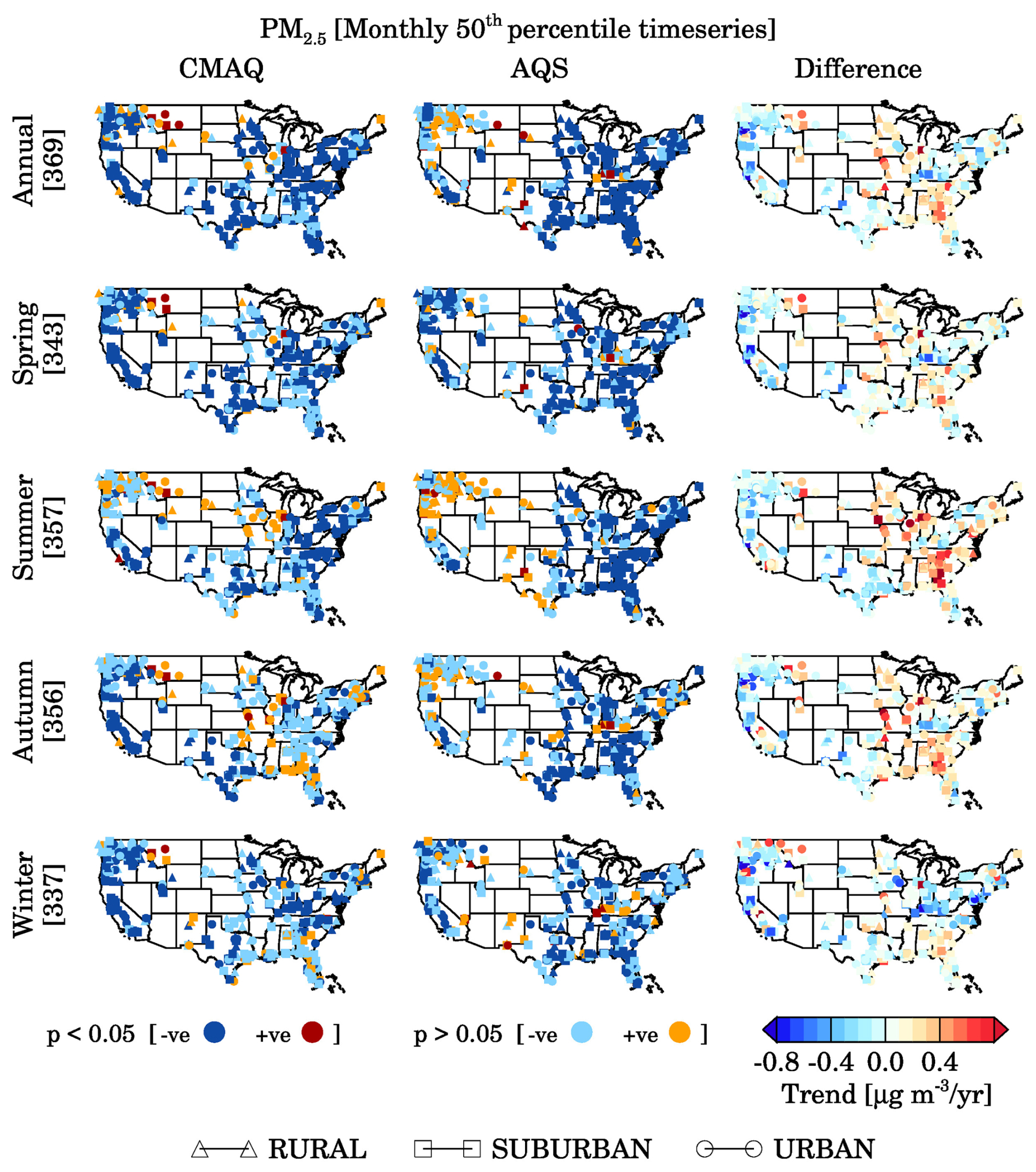
Figure 10 Spatial distribution of positive (blue colors) and negative (red colors) trends in the 24 h mean PM_2.5 (right panel) at different levels of statistical significance (p values) using monthly median time series (top to bottom). Plots on the right show the differences in trend values (CMAQ − AQS).

On an annual basis, the mean PM_2.5 trends for the respective AQS and CMAQ datasets are −0.17 ± 0.22 and −0.18 ± 0.15 µg m⁻³ yr⁻¹ over urban sites, −0.28 ± 0.22 and −0.24 ± 0.26 µg m⁻³ yr⁻¹ over suburban sites, and −0.23 ± 0.21 and −0.30 ± 0.27 µg m⁻³ yr⁻¹ over urban and city center sites. The only high-altitude site for PM_2.5 showed an increase in the annual trend (0.07 and 0.06 µg m⁻³ yr⁻¹ for AQS and CMAQ data, respectively) and the summertime trend (0.13 and 0.13 µg m⁻³ yr⁻¹ for AQS and CMAQ data, respectively). During other seasons, mostly low negative trends were observed. The ozone trends over high-altitude sites (16 sites), however, are mostly negative (−0.43 ± 0.45 and −0.12 ± 0.36 ppb yr⁻¹ in summer and −0.39 ± 0.38 and −0.03 ± 0.29 ppb yr⁻¹ annually). The ozone trends at high-altitude sites showed large seasonal variations with minimum to maximum ranges of −0.69 to 0.87 and −1.5 to 0.26 ppb yr⁻¹ for AQS and CMAQ data, respectively.

4.4 Air quality dashboard

The comprehensive evaluation of our reanalysis in the above sections shows that our reanalysis is able to capture key features of long-term trends in both MDA8 ozone and PM_2.5 over most parts of the CONUS. This increases confidence in using this dataset for assessing the trends in unmonitored areas of the region. Therefore, a GIS-based dashboard has been developed to aid in community engagement and understanding of the reanalysis data. The dashboard was developed using ArcGIS Dashboards technology from Esri (https://www.esri.com/en-us/arcgis/products/arcgis-dashboards/overview, last access: 28 April 2025). An interactive web-based dashboard allows stakeholders to explore annual air quality concentrations and the number of days that exceed a certain threshold over space and time. It provides a step-by-step path for users to explore information at the CONUS, state, and county levels. In the center of the dashboard is a time series chart showing trends in annual concentrations of MDA8 ozone, NO₂, PM_2.5, PM₁, and PM₁₀ between 2005 and 2018. An indicator element of the dashboard highlights how many days between 2005 and 2018 have exceeded the National Ambient Air Quality Standards (NAAQS) for ozone and PM_2.5, and a bar chart graph shows the number of days that exceeded the NAAQS each year. There is also a map that can zoom in on the selected state or county of interest and illustrates the spatial distribution of air quality variables using a quantitative color bar.

The dashboard can be used to better understand how particular events, such as large wildfires, have affected air quality in certain geographic areas. For example, the 2008 wildfires in Shasta and Trinity counties in California, referred to as the “June Fire Siege”, had a major impact on air quality (https://storymaps.arcgis.com/stories/c6535ee477e14b72a20393a5f10aefbc, last access: 28 April 2025). Figure 11 shows MDA8 ozone concentrations for Shasta County, California. The dashboard shows a sharp increase in the MDA8 ozone concentration in 2008, as depicted in the time series plot. The bar chart in the lower right-hand corner also reflects the large number of days that exceeded the NAAQS criteria for MDA8 ozone in 2008.

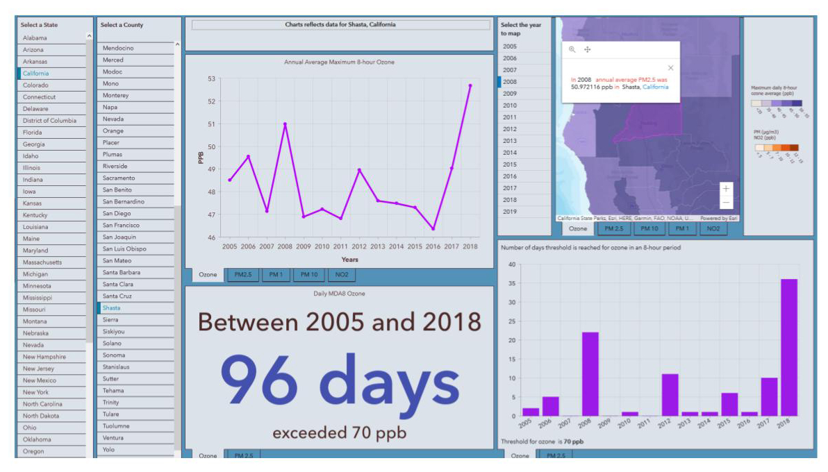
Figure 11 Dashboard reflecting ozone concentrations for Shasta County, CA.

The dashboards can also be used to visualize the efficacy of air quality management policies. For example, Los Angeles County, CA, has designed and implemented strict emission standards to improve air quality. Figure 12 shows the downward trend in PM_2.5 concentrations in Los Angeles County during 2005–2018. The air quality dashboard is publicly accessible at https://ncar.maps.arcgis.com/apps/dashboards/9a97650dc77b4f7192b99ea9bef36a21 (last access: 28 April 2025). To ensure stakeholders have an understanding of the uncertainties, we have included the following message on the website: “Note that mean bias of 3.7–6.8 ppbv in ozone and that of −0.9–5.6 µg m⁻³ in PM_2.5 could have impacted the calculation of days exceeding the corresponding National Ambient Air Quality Standards”.

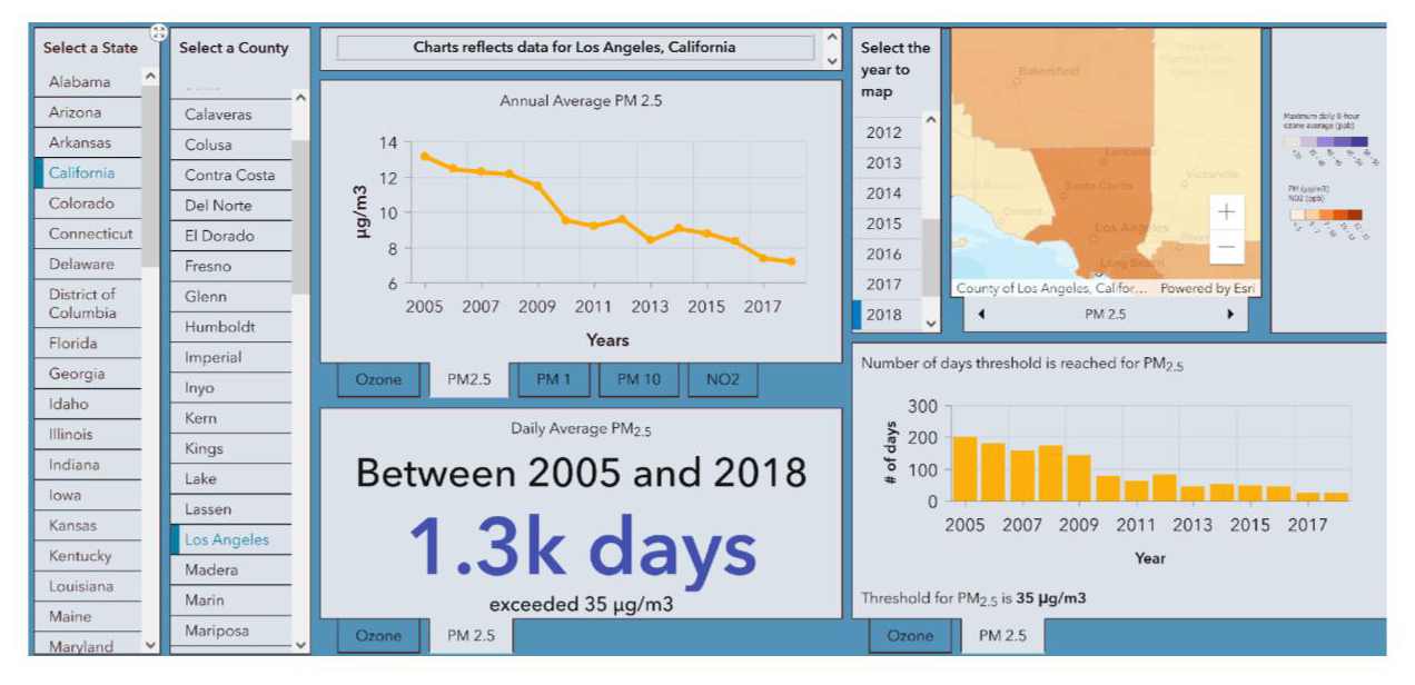
Figure 12 Dashboard reflecting PM_2.5 concentrations for Los Angeles, CA.

We have also developed a Python-based Streamlit application that allows users to select and download data for specific time periods aggregated over administrative boundaries such as cities, counties, and states. Temporal and spatial aggregations are performed on the server, and only information of interest is downloaded and delivered to the users, taking the data processing workload off of the users. The Streamlit application allows users to select a time period, a temporal aggregation (daily, weekly, monthly, or annual), one or more air quality variables, statistics (min, mean, or max), and an area of interest (state, county, or city). The data can then be downloaded as a comma-separated value (CSV) file as well as graphed on the website, as seen in Fig. 13. The Streamlit application is available at https://compass.rap.ucar.edu/airquality/ (last access: 28 April 2025).

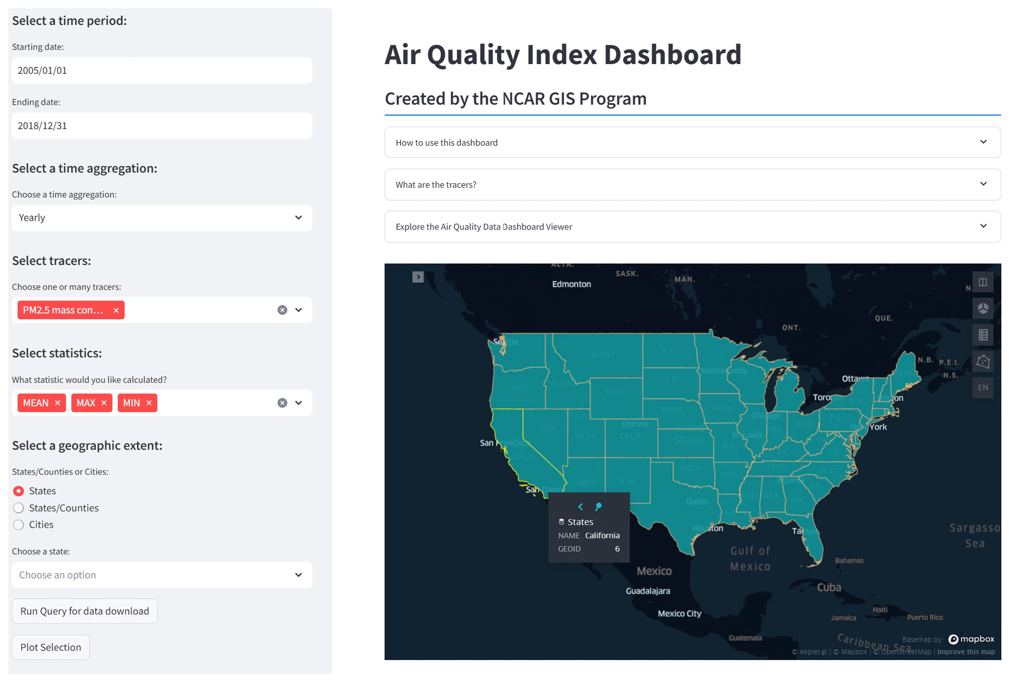
Figure 13 The Streamlit air quality app to easily download and summarize data in a CSV format.

5 Data availability

The global meteorological datasets used to drive WRF are publicly available through the National Center for Atmospheric Research (NCAR) Research Data Archive (https://doi.org/10.5065/D6CR5RD9, European Centre for Medium-Range Weather Forecasts, 2009). The SMOKE setup used to create emissions for CMAQ is accessible via the EPA Emissions Modeling Platforms (https://gaftp.epa.gov/air/emismod/2011/v3platform/, EPA, 2011; https://gaftp.epa.gov/air/emismod/2014/v2/, EPA, 2014; https://gaftp.epa.gov/Air/emismod/2017/, EPA, 2017). FINN biomass burning emissions can be downloaded from https://doi.org/10.5065/XNPA-AF09 (Wiedinmyer and Emmons, 2022). Meteorological observations used to evaluate the model performance are available from https://madis-data.cprk.ncep.noaa.gov/madisPublic1/data/archive/ (NOAA, 2025). The EPA AQS system observations are available from https://www.epa.gov/aqs (US EPA, 2025). Hourly surface output from the WRF-CMAQ-GSI system can be downloaded from https://doi.org/10.5065/cfya-4g50 (Kumar and He, 2023).

6 Code availability

The WRF code is publicly accessible at https://github.com/wrf-model/WRF (Islas, 2025). The CMAQ code is publicly accessible at https://github.com/USEPA/CMAQ (Adams, 2025), and the GSI code is available at https://github.com/NOAA-EMC/GSI (Liu, 2025).

7 Conclusions

Air pollution is an important health hazard affecting human health and the economy in the CONUS, yet millions of people live in counties without air quality monitors. To address this gap and help air quality managers understand long-term changes in air quality at the county level across the CONUS, we have created a 14-year-long, 12 km, hourly dataset via the daily assimilation of atmospheric composition observations from the NASA MODIS and MOPITT sensors aboard the Terra and Aqua satellites in the Community Multiscale Air Quality (CMAQ) model from 1 January 2005 to 31 December 2018. The WRF model has been used to simulate meteorological parameters, which are then used to drive CMAQ offline and to generate meteorology-dependent anthropogenic emissions.

The meteorological parameters, ozone, and PM_2.5 have been extensively validated against multi-platform observations to characterize uncertainties in our dataset, which air quality managers need to determine the confidence that they can put in our dataset. We show that our dataset captures regional-scale hourly, seasonal, and interannual variability in the meteorological variability well across the CONUS. The model shows excellent performance with respect to simulating the regional and temporal variability in temperature and relative humidity but slightly poorer performance with respect to simulating winds and precipitation, which are well-known shortcomings of the WRF model. The model also shows a higher skill with respect to reproducing variabilities in surface ozone (r = 0.77–0.91) compared with PM_2.5 (0.49–0.79). The mean biases for CMAQ ozone and PM_2.5 are estimated to be 3.7–6.8 ppbv and −0.9–5.6 µg m⁻³, respectively, and the corresponding RMSE values are 7–9 ppbv and 3.0–8.3 µg m⁻³, respectively.

The MDA8 ozone trend over the CONUS is estimated to be −0.53 ± 0.46 and −0.56 ± 0.45 ppb yr⁻¹ (summertime) and −0.31 ± 0.43 and −0.29 ± 0.39 ppb yr⁻¹ (annual) for AQS and CMAQ data, respectively, with ∼ 70 % of sites showing negative trends. At the 2σ level, the summertime MDA8 ozone trends are −0.85 ± 0.36 and −0.75 ± 0.35 ppb yr⁻¹ and the annual MDA8 ozone trends are −0.52 ± 0.45 and −0.47 ± 0.42 ppb yr⁻¹ for AQS and CMAQ data, respectively, over the CONUS. Annually, at the 2σ level, 46 % sites showed negative trends in both of the datasets. Annual mean PM_2.5 trends are −0.24 ± 0.21 and −0.24 ± 0.24 µg m⁻³ yr⁻¹ in the AQS and CMAQ datasets, respectively, and ∼ 79 % of the sites showed negative trends. Annually, at the 2σ level, 66 % of sites showed negative trends in both of the datasets. During summertime, the negative trend percentage is reduced to 71 %, where an increase in positive trends is observed in the northwestern US.

An air quality dashboard has been developed that provides a step-by-step path for users to explore information at the CONUS, state, and county levels. This dashboard allows users to visualize air quality information in the form of maps, bar charts, and NAAQS exceedance days. Finally, a Python-based Streamlit application is developed to allow the download of air quality data in simplified text and graphic formats for the end user's choice of region and time of interest.

Appendix A

A1 Forward and adjoint operators for MOPITT CO assimilation

The MOPITT-retrieved profile consists of 10 levels, including a surface level followed by 100 hPa thick layers from 900 to 100 hPa. The CMAQ vertical profile of CO cannot be compared with MOPITT CO directly and needs to be convolved with the MOPITT a priori profile and averaging kernel. Following Barré et al. (2015) and Gaubert et al. (2016), the CMAQ profile that can be compared directly to MOPITT can be written as follows:

$$\begin{array}{}\text{(A1)}& \begin{array}{rl}& {\mathrm{CO}}_{\mathrm{ret}}^{\mathrm{CMAQ}}=\\ & {\mathrm{10}}^{\left({\mathrm{AK}}^{\mathrm{MOPITT}}{\log }_{\mathrm{10}}\right({\mathrm{CO}}^{\mathrm{CMAQ}})+(I-{\mathrm{AK}}^{\mathrm{MOPITT}}\left){\log }_{\mathrm{10}}\right({\mathrm{CO}}_{\mathrm{apr}}^{\mathrm{MOPITT}}\left)\right).}\end{array}\end{array}$$

Here, ${\mathrm{CO}}_{\mathrm{ret}}^{\mathrm{CMAQ}}$ is the CMAQ CO profile convolved with the MOPITT a priori averaging kernel (AK^MOPITT) and a priori profile (${\mathrm{CO}}_{\mathrm{apr}}^{\mathrm{MOPITT}}$) that can be compared directly to the MOPITT retrieved CO profile. CO^CMAQ is the 10-layer CMAQ profile mapped to the MOPITT pressure grid. A log₁₀ transformation is necessary because the averaging kernel matrix for retrievals is obtained with CO parameters in log₁₀(CO). Differentiation of Eq. (1) will yield the sensitivity of ${\mathrm{CO}}_{\mathrm{ret}}^{\mathrm{CMAQ}}$ with respect to CO^CMAQ, which represents the adjoint of the forward operator. For the purpose of derivation, let ${\mathrm{CO}}_{\mathrm{ret}}^{\mathrm{CMAQ}}=y$, CO^CMAQ=x, AK^MOPITT = A, and $(I-{\mathrm{AK}}^{\mathrm{MOPITT}}){\log }_{\mathrm{10}}\left({\mathrm{CO}}_{\mathrm{apr}}^{\mathrm{MOPITT}}\right)=C$. Equation (1) can be written as follows:

$$\begin{array}{}\text{(A2)}& y={\mathrm{10}}^{\left(A{\log }_{\mathrm{10}}\right(x)+C)}.\end{array}$$

Applying the differentiation rule $\frac{\mathrm{d}\left[a^u\right]}{\mathrm{d}x}=\ln \left(a\right)\cdot a^u\cdot \frac{\mathrm{d}u}{\mathrm{d}x}$, we can differentiate Eq. (2) as follows:

$$\begin{array}{}\text{(A3)}& {\displaystyle \frac{\mathrm{d}y}{\mathrm{d}x}}=\ln \left(\mathrm{10}\right)\cdot {\mathrm{10}}^{\left(A{\log }_{\mathrm{10}}\right(x)+C)}\cdot {\displaystyle \frac{\mathrm{d}}{\mathrm{d}x}}\left(A{\log }_{\mathrm{10}}\right(x)+C).\end{array}$$

As A and C do not depend on CMAQ simulations, they are constants; thus, their differentiation is zero. As $\frac{\mathrm{d}}{\mathrm{d}x}\left({\log }_{\mathrm{10}}\right(x\left)\right)=\frac{\mathrm{1}}{x\ln \left(\mathrm{10}\right)}$, Eq. (3) simplifies to the following:

$$\begin{array}{}\text{(A4)}& {\displaystyle \frac{\mathrm{d}y}{\mathrm{d}x}}={\mathrm{10}}^{\left(A{\log }_{\mathrm{10}}\right(x)+C)}\cdot A\cdot {\displaystyle \frac{\mathrm{1}}{x}}=A\cdot {\displaystyle \frac{y}{x}}.\end{array}$$

Substituting the values of $y,x,A,$ and  C in Eq. (4), the changes in the CO vertical profile in the MOPITT space can be related to changes in CO vertical profile in CMAQ as follows:

$$\begin{array}{}\text{(A5)}& {\mathrm{dCO}}_{\mathrm{ret}}^{\mathrm{CMAQ}}={\mathrm{AK}}^{\mathrm{MOPITT}}\cdot {\displaystyle \frac{{\mathrm{CO}}_{\mathrm{ret}}^{\mathrm{CMAQ}}}{{\mathrm{CO}}_{}^{\mathrm{CMAQ}}}}{\mathrm{dCO}}^{\mathrm{CMAQ}}.\end{array}$$

By writing Eq. (5) in matrix form and then transposing the forward-operator matrix, we can write the adjoint of the forward operator as a recursive matrix equation:

$$\begin{array}{}\text{(A6)}& \begin{array}{rl}{\mathrm{dCO}}^{\mathrm{CMAQ}}& ={\mathrm{dCO}}^{\mathrm{CMAQ}}+{\mathrm{AK}}^{\mathrm{MOPITT}}\\ & \cdot {\displaystyle \frac{{\mathrm{CO}}_{\mathrm{ret}}^{\mathrm{CMAQ}}}{{\mathrm{CO}}^{\mathrm{CMAQ}}}}{\mathrm{dCO}}_{\mathrm{ret}}^{\mathrm{CMAQ}}.\end{array}\end{array}$$

A2 Additional figures

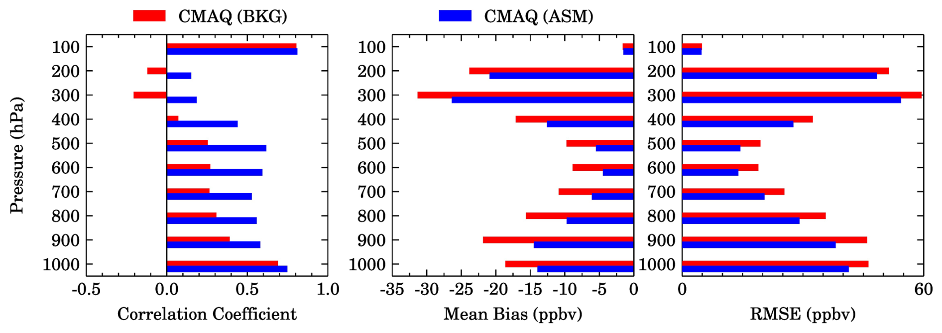
Figure A1 The correlation coefficient, mean bias, and root-mean-square error (RMSE) between the CMAQ and MOPITT CO profiles at 10 MOPITT retrieval pressure levels for the CMAQ experiments with (ASM) and without (BKG) assimilation of the MOPITT CO profiles during July 2018. These statistics are based on 118 552 data points at each level.

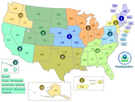
Figure A2 Map showing the EPA regions over which model evaluation has been performed. The map is reproduced from https://www.epa.gov/aboutepa/visiting-regional-office (last access: 28 April 2025). Our evaluation does not include Puerto Rico in Region 2, the Hawaiian Islands in Region 9, and Alaska in Region 10.

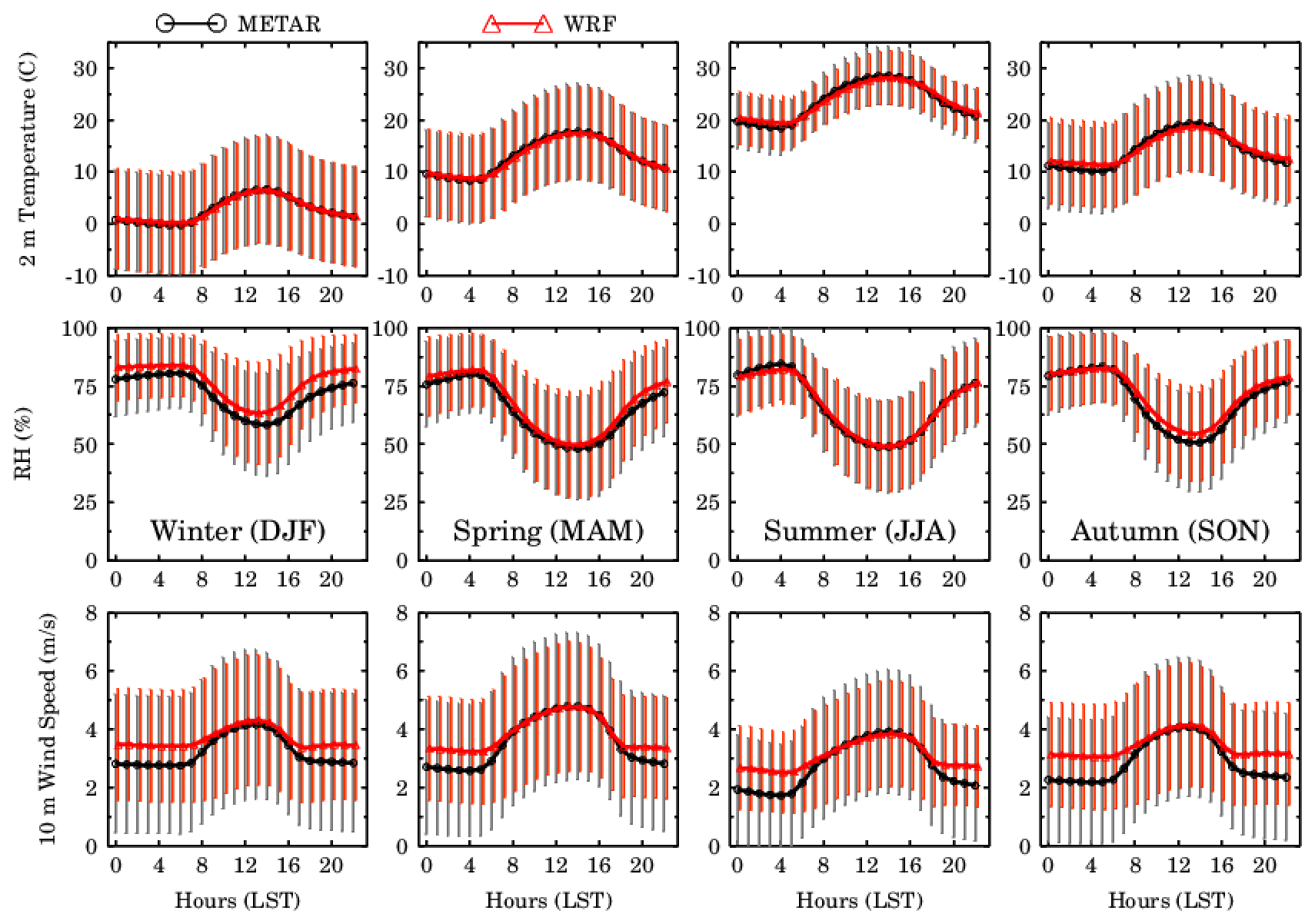
Figure A3 Seasonal mean diurnal variations in 2 m temperature (top row), relative humidity (middle row), and 10 m wind speed (bottom row) from METAR observations and the WRF model.

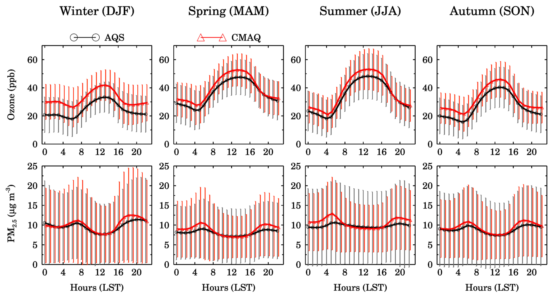
Figure A4 Average diurnal profile of ozone (top row) and PM_2.5 (bottom row) over all AQS sites in the CONUS.

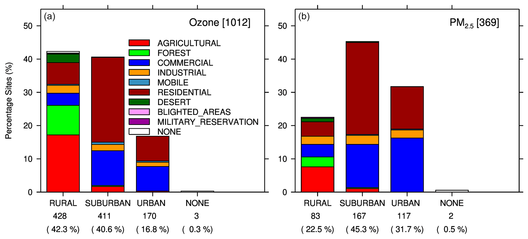
Figure A5 The stacked histogram shows the number of sites in each location setting (different bars) and land use type (different colors) for MDA8 ozone (a) and 24 h mean PM_2.5 (b).

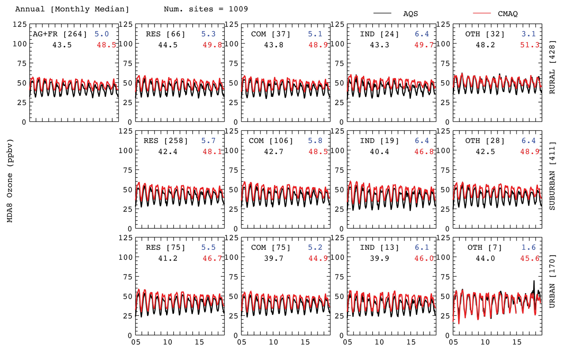
Figure A6 The annual mean (derived from monthly median values) time series of MDA8 ozone using AQS data (black) and the CMAQ (red) over different location (top to bottom) and land use (left to right) types during the period from 2005 to 2018. The number of sites for each scenario is presented in brackets. The blue color represents the mean bias.

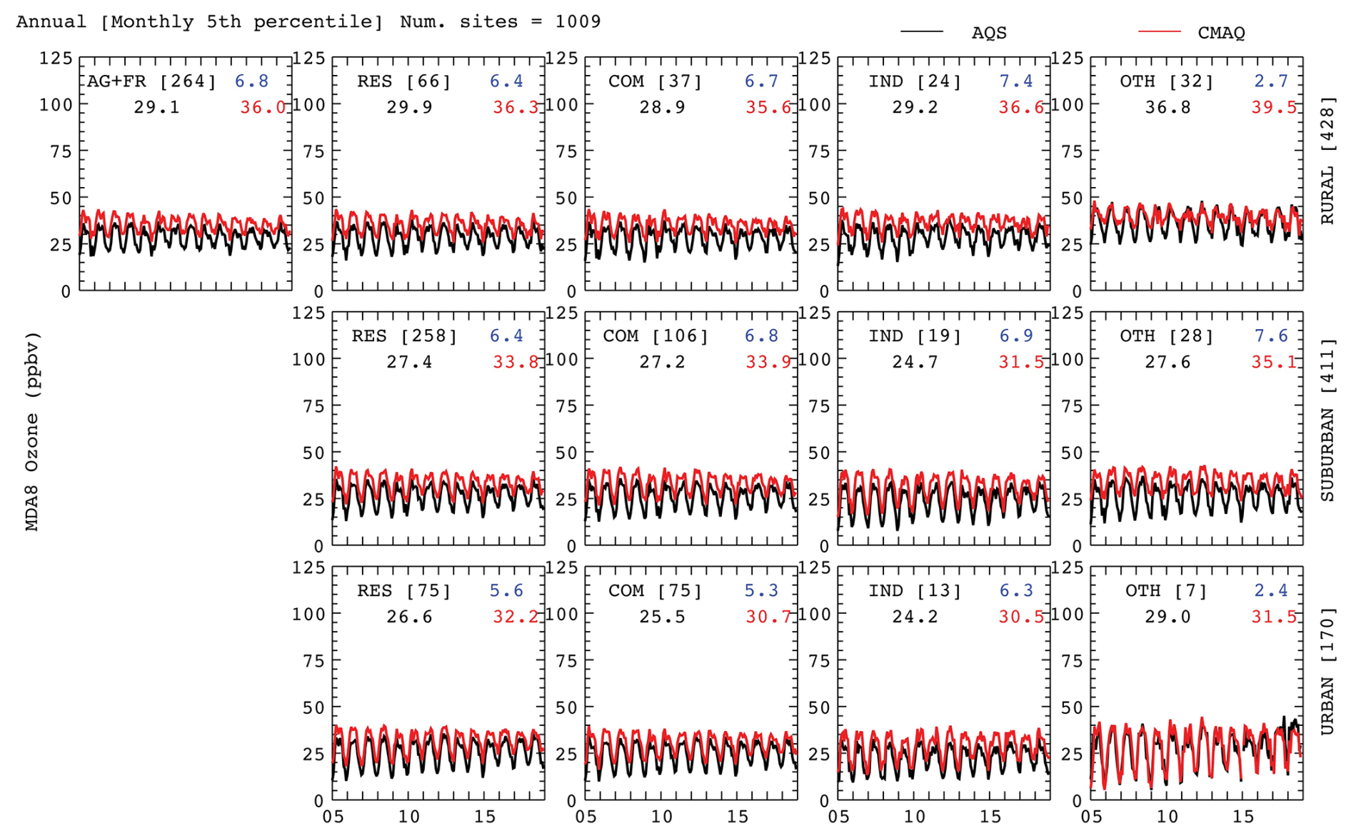
Figure A7 Same as Fig. A6 but for time series derived from the monthly 5th percentile values.

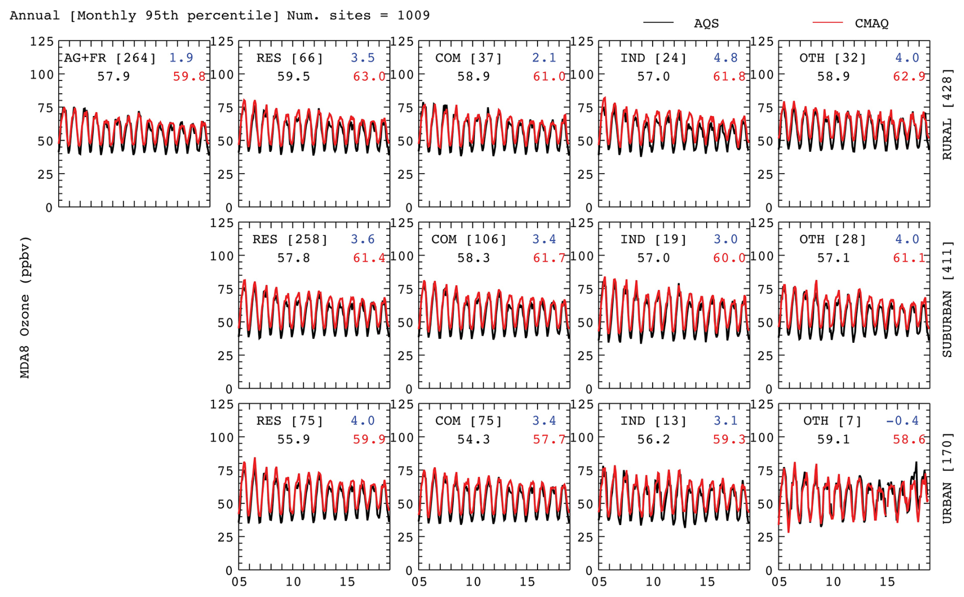
Figure A8 Same as Fig. A6 but for time series derived from the monthly 95th percentile values.

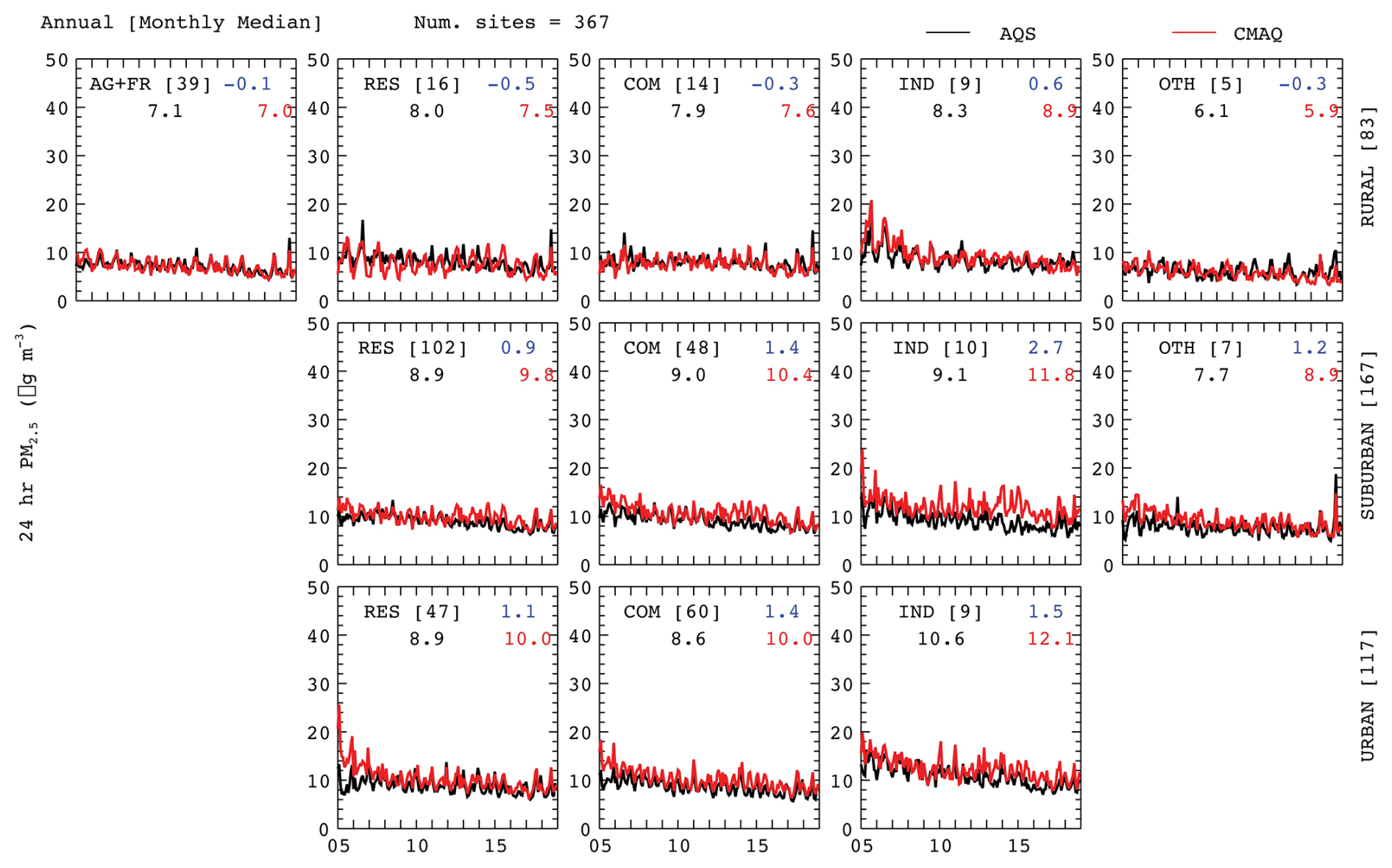
Figure A9 The annual mean (derived from monthly values) time series of 24 h mean PM_2.5 using AQS data (black) and the CMAQ (red) over different location (top to bottom) and land use (left to right) types during the period from 2005 to 2018. The number of sites for each scenario is presented in brackets. The blue color represents the mean bias.

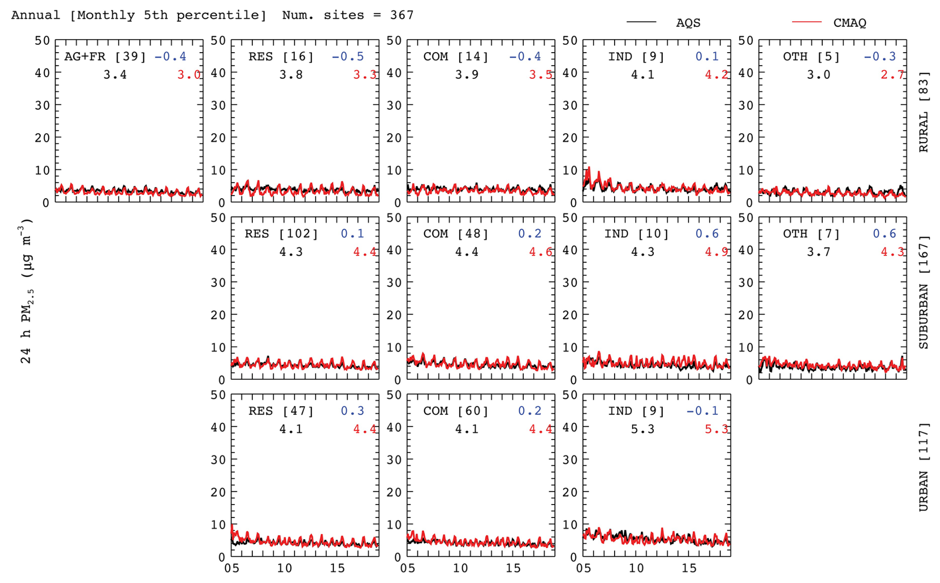
Figure A10 Same as Fig. A9 but for time series derived from the monthly 5th percentile values.

Figure A11 Same as Fig. A9 but for time series derived from monthly 95th percentile values.

A3 Additional tables

Table A1 Key physics and chemical schemes used in the WRF-CMAQ configuration.

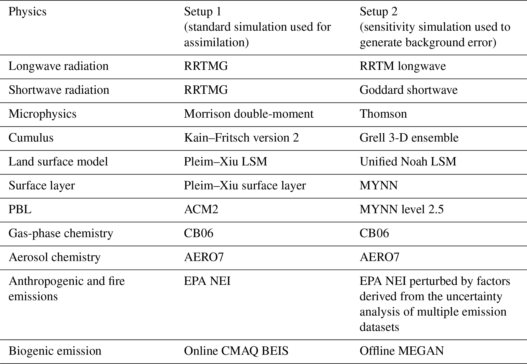
LSM denotes land surface model.

Table A2 Annual anthropogenic emissions (in Tg yr⁻¹) for nine species over the CONUS during the period from 2005 to 2018.

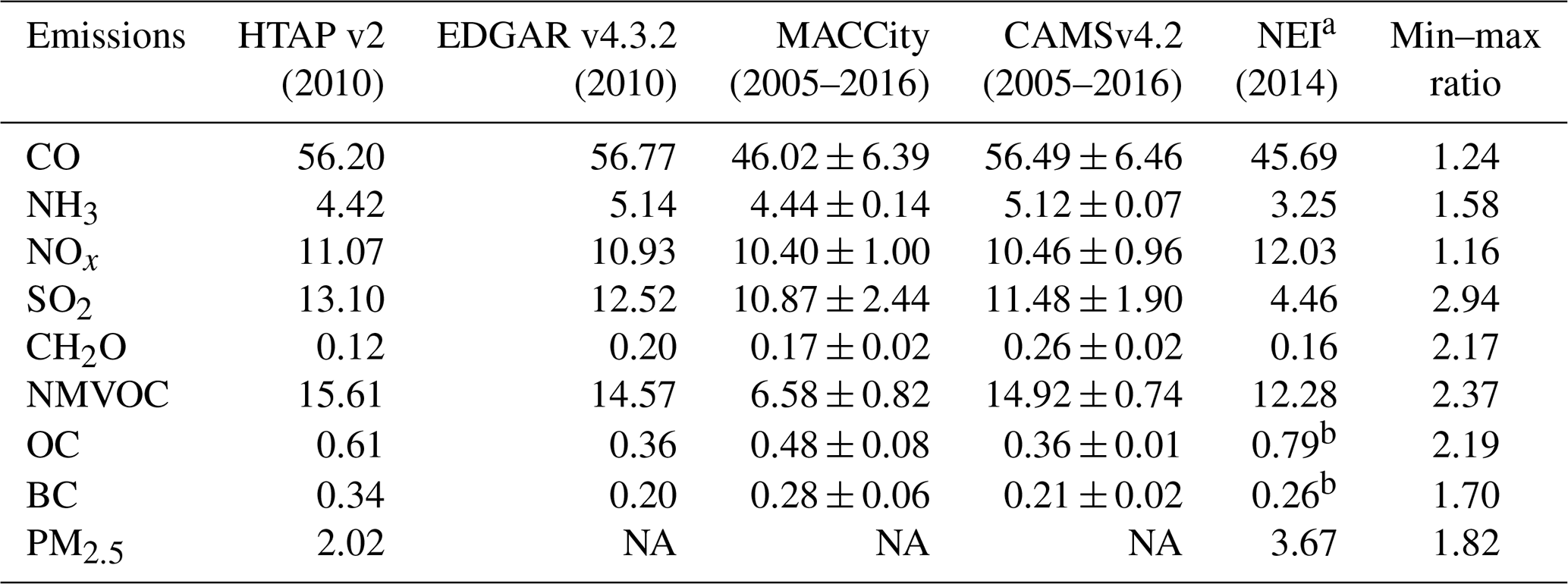
^a Except for NEI, all other emissions are simply summed over the region between 20 and 50°N and between 60 and 130° W. ^b The CONUS PM_2.5 emissions are 5.15 Tg yr⁻¹ and comprise 8 % BC (or EC) and 28 % OC (https://www.epa.gov/sites/production/files/2019-08/documents/210pm_rao_508_2.pdf, last access: 28 April 2025). The abbreviations used in the table are as follows: non-methane volatile organic compounds (NMVOC), black carbon (BC), organic carbon (OC), elemental carbon (EC), and not available (NA).

Table A3 Annual biomass burning emissions (in Tg yr⁻¹) for nine species over the CONUS during the period from 2005 to 2018.

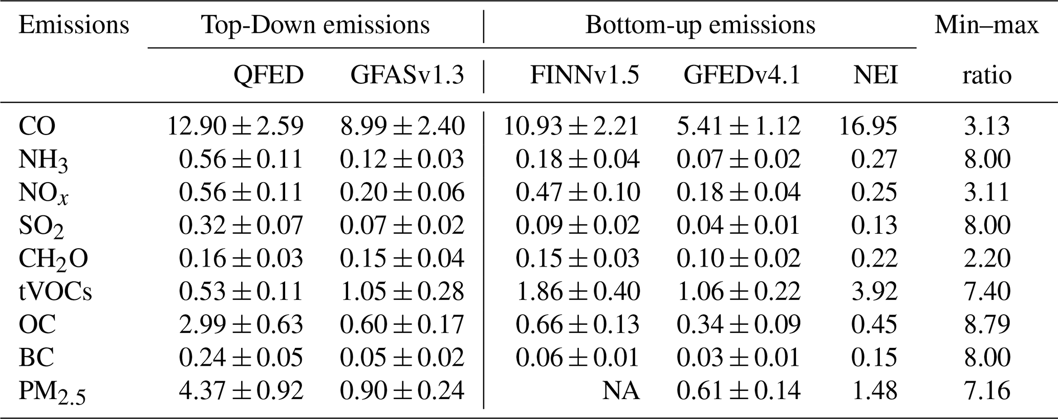
The abbreviations used in the table are as follows: total volatile organic compounds (tVOCs), black carbon (BC), organic carbon (OC), elemental carbon (EC), and not available (NA).