SDUST2023BCO: a global seafloor model determined from a multi-layer perceptron neural network using multi-source differential marine geodetic data

Seafloor topography, as a fundamental marine spatial geographic information, plays a vital role in marine observation and science research. With the growing demand for high-precision bathymetric models, a multi-layer perceptron (MLP) neural network is used to integrate multi-source marine geodetic data in this paper. A new bathymetric model of the global ocean, spanning 180° E–180° W and 80° S–80° N, known as the Shandong University of Science and Technology 2023 Bathymetric Chart of the Oceans (SDUST2023BCO), has been constructed, with a grid size of 1^′ × 1^′. The multi-source marine geodetic data used include gravity anomaly data released by the Shandong University of Science and Technology, the vertical gravity gradient and the vertical deflection data released by the Scripps Institution of Oceanography (SIO), and the mean dynamic topography data released by Centre National d'Etudes Spatiales (CNES). First, input and output data are organized from the multi-source marine geodetic data to train the MLP model. Second, the input data at interesting points are fed into the MLP model to obtain prediction bathymetry. Finally, a high-precision bathymetric model with a resolution of 1^′ × 1^′ has been constructed for the global marine area. The validity and reliability of the SDUST2023BCO model are evaluated by comparing with shipborne single-beam bathymetric data and GEBCO_2023 and topo_25.1 models. The results demonstrate that the SDUST2023BCO model is accurate and reliable, effectively capturing and reflecting global marine bathymetric information. The SDUST2023BCO model is available at https://doi.org/10.5281/zenodo.13341896 (Zhou et al., 2024).

1 Introduction

As a critical foundational dataset for marine scientific research, global bathymetric information plays a vital role in multiple disciplines such as marine geodesy, geophysics, biology and seafloor geology. It is also essential for marine economic development, oceanographic surveys, maritime navigation and rescue operations (Hirt and Rexer, 2015; Hu et al., 2015; Yang et al., 2018; Sandwell et al., 2022). Currently, shipborne single-beam bathymetric techniques can provide high-precision bathymetric data, which is one of the most direct ways of detecting seafloor topography. However, despite the accumulation of data collected through shipborne techniques, large areas of the global oceans, especially in the Southern Hemisphere, remain largely uncharted (Hu et al., 2014). Moreover, shipborne single-beam bathymetric data, characterized by its low resolution, high expenses and low precision in positioning and measurements of older datasets, present significant limitations (Hu et al., 2014; Xing et al., 2020). The progression in satellite altimetry technology has ushered in a novel era for the development of bathymetric models. Satellite altimetry, as one of the critical techniques for acquiring global marine data, can obtain the global-coverage, uniformly distributed, high-precision and high-resolution sea surface heights. The global marine gravity field information can be recovered based on relevant geodetic methods (Marks and Smith, 2012; Sun et al., 2021; Kim et al., 2011). The global bathymetric model can be obtained with seafloor-inversion methods, considering the inherent correlation between seafloor topography and global marine gravity information (Wang, 2000; Hu et al., 2021; Yeu et al., 2018).

Currently, the inversion of bathymetric values based on marine gravity data acquired from satellite altimeter data has become a reliable approach to construct global bathymetric models. The methods employed for predicting seafloor topography based on satellite altimeter data mainly include frequency-domain methods, spatial-domain methods (analytical methods), least-squares collocation methods and gravity-geological methods (GGMs). While high-precision bathymetric models have been effectively constructed using these methods for specific regions, such as the South China Sea (Fan et al., 2020; An et al., 2022; Hu et al., 2020), western Pacific Ocean (Yang et al., 2018), Gulf of Guinea (Annan and Wan, 2020), Philippine Sea (An et al., 2024) and New Zealand (Ramillien and Wright, 2000), the nonlinear relationship between gravity data and seafloor topography is still not adequately used by these methods. At the same time, the seafloor topography is constructed solely based on the linear relationship between the gravity anomalies or vertical gravity gradients and the seafloor topography. Consequently, a global bathymetric model can be constructed by integrating the nonlinear components inherent in the relationship between the multi-source marine geodetic data and the seafloor topography. At the same time, the long-wavelength information in multi-source marine geodetic data will affect the prediction accuracy of seafloor topography models. Therefore, it is necessary to mitigate the impact of long-wavelength information on the accuracy of model establishment.

With the continuous advancement in computer storage and computational capabilities, machine learning or deep learning has been widely applied in various scientific fields, such as environmental science (Sunil et al., 2024), geology (Kuster and Toksoz, 1974) and clinical medicine (Lee et al., 2019). Currently, machine learning or deep learning methods are increasingly used to construct bathymetric models. Sun et al. (2023) proposed a method combining neural networks and wavelet decomposition of gravity information, and the superiority of this method has been validated. However, this model only used gravity anomaly and vertical gravity gradient data without considering other multi-source marine geodetic data. Zhou et al. (2023) used a multi-layer perceptron (MLP) neural network with a regional inversion approach to construct a high-precision bathymetric model of the Gulf of Mexico. However, the impact of long-wavelength information from multi-source marine geodetic data on the accuracy of the constructed bathymetric model was not considered.

The focus of this paper is the establishment of a new global (80° S–80° N, 180° E–180° W) bathymetric model, named Shandong University of Science and Technology 2023 Bathymetric Chart of the Oceans (SDUST2023BCO). This model is constructed based on an MLP neural network using the differences between the multi-source marine geodetic data (gravity anomalies, vertical gravity gradients, meridional and prime components of vertical deflection, mean dynamic topography) of training/prediction points, and their surrounding grid points. The reliability of SDUST2023BCO model is validated by comparing it with the GEBCO_2023 and topo_25.1 models. Section 2 introduces the multi-source marine geodetic data used in this paper. Section 3 explains the processing methods for the shipborne single-beam bathymetric data, the principle of the MLP neural network, the organization of input/output data and the procedure for constructing the bathymetric model. Section 4 contains the results and discussions. By comparing it with the shipborne single-beam bathymetric data, the GEBCO_2023 model and the topo_25.1 model, the SDUST2023BCO model is verified. Section 5 contains the conclusion.

2 Data

The global ocean (80° S–80° N, 180° E–180° W) is designated as the study region in this paper. Due to the limitations in computational power and storage capacity, the study region is divided into 144 sub-regions, as shown in Fig. 1. From west to east, the area is divided into 18 columns and marked as LONG1 to LONG18. From north to south, the region is divided into eight rows and marked as LAT1 to LAT8. To mitigate edge effects and stitching issues between different sub-regions, each sub-region is expanded by 0.1° in all directions. The extended data are used for the inversion of seafloor topography.

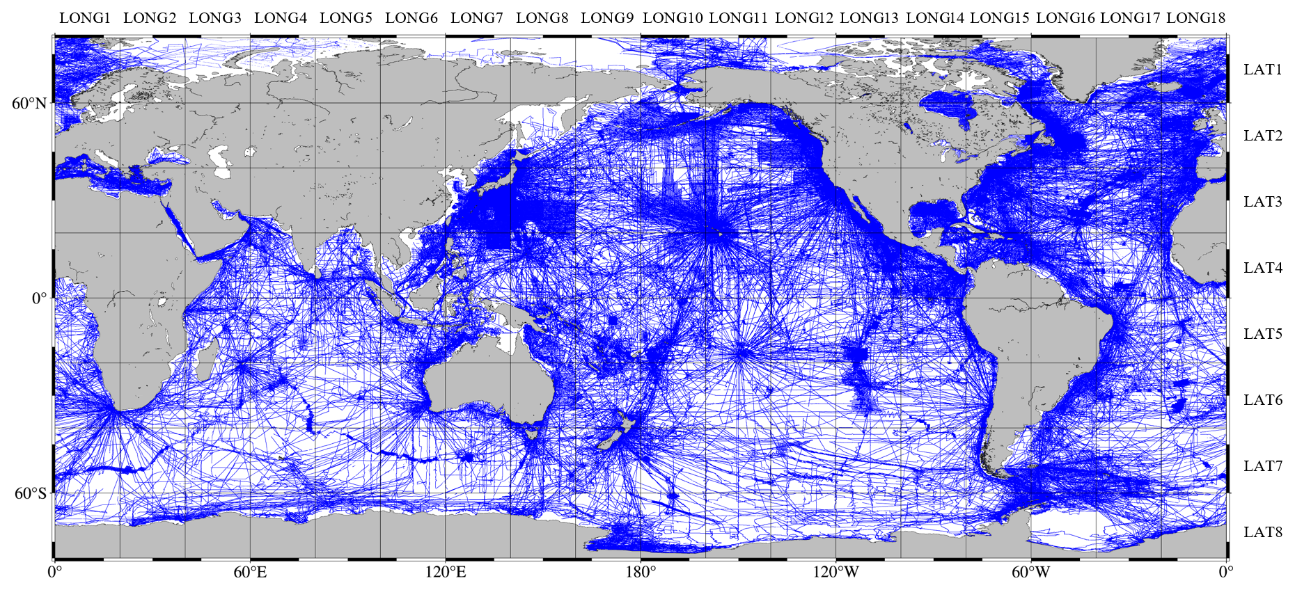
Figure 1 Division map and the distribution of shipborne single-beam bathymetry data.

2.1 Shipborne single-beam bathymetry data

The shipborne single-beam bathymetry data are provided by the National Centers for Environmental Information (NCEI), a division of the National Oceanic and Atmospheric Administration (NOAA) in the United States. The dataset contains global marine bathymetric data collected since the 1950s. The study region includes 5374 shipborne single-beam bathymetry tracks, as shown in Fig. 1.

Owing to the large time span of the shipborne single-beam bathymetric data, some datasets have imprecise localization and significant measurement inaccuracies. Therefore, it is necessary to preprocess the data to remove some points with substantial errors. Now, the global marine bathymetric models derived from satellite altimetry data achieve a high level of accuracy. The topo_25.1 model, as the latest bathymetric model released by the Scripps Institution of Oceanography (SIO), shows a standard deviation (SD) of approximately 435 m compared to global shipborne single-beam bathymetric data. Therefore, this paper uses the topo_25.1 model as a prior model to remove shipborne single-beam bathymetric points with significant errors. The process of elimination primarily consists of two parts:

The first step is to remove shipborne single-beam bathymetric tracks that contain significant errors. First, the topo_25.1 model is used to calculate the predicted bathymetry at each shipborne single-beam bathymetric point using a cubic spline interpolation method. The difference between the topo_25.1 predicted bathymetric values and the actual measured bathymetry at each point is calculated, and the standard deviation (SD1) of these differences is calculated. Second, the topo_25.1 model is interpolated onto each shipborne single-beam bathymetric track to obtain corresponding bathymetry. The differences between these interpolated values and the actual measured depths along each track are calculated, and the SD of these differences is computed for each track. Finally, the entire shipborne single-beam bathymetric track is removed if its SD exceeds SD1 3 times. Using this method, 38 ship tracks with significant errors are eliminated, leaving 5336 shipborne single-beam bathymetric tracks, which consist of a total of 11 335 376 shipborne single-beam bathymetric points.

The second step is to remove shipborne single-beam bathymetric points with large errors. Despite the initial removal of entire tracks, some individual shipborne single-beam bathymetric points with significant large errors may still remain. Therefore, the method is employed to eliminate shipborne single-beam bathymetric points that exhibit significant errors. First, the topo_25.1 model is interpolated onto all the remaining shipborne single-beam bathymetric points to obtain the topo_25.1 predicted bathymetry at these points. The difference between the topo_25.1 predicted bathymetry and the actual measured bathymetry at each point is calculated. The SD of these differences is calculated and shipborne single-beam bathymetric points with absolute bathymetric residuals greater than 3 times the SD are removed. Finally, the 1 016 374 shipborne single-beam bathymetric points are eliminated, leaving 112 319 002 shipborne single-beam bathymetric points, with a removal rate of 0.90 %. The 112 319 002 shipborne single-beam bathymetric points are used to train the MLP model which is employed to construct the SDUST2023BCO model. Among them, the largest shipborne single-beam bathymetric data are 10 949.5 m, and the average bathymetry is 2819.8 m.

2.2 Marine geodetic data

2.2.1 Marine gravity data

Gravity anomaly data originate from the global gravity anomaly model (SDUST2022GRA) constructed by the Shandong University of Science and Technology in 2022. This model is constructed based on the along-track radar altimeter data (Li et al., 2024), and the accuracy and reliability of this model have been verified by comparing with the DTU17 model, SIO grav_32.1 model and shipborne gravity data from NCEI. In local coastal and high-latitude regions, SDUST2022GRA showed an enhancement of 0.16–0.24 mGal compared to the altimeter-derived global gravity anomaly models (DTU17, V32.1, NSOAS22) and shipborne gravity measurements. The model is available for download from https://doi.org/10.5281/zenodo.8337387 (Li et al., 2023), with a resolution of 1^′ × 1^′.

Based on the correlation between vertical deflection, vertical gravity gradient and bathymetry, those data can also be utilized to predict bathymetry. These gravity data are derived from version 32.1 released by SIO in 2022, with a resolution of 1^′ × 1^′, and can be freely obtained from https://topex.ucsd.edu/pub/global_grav_1min/ (last access: 10 August 2024).

2.2.2 MDT model

The mean dynamic topography (MDT) model used in this study is the MDT-CNES-CLS18 model released by the Centre National d'Etudes Spatiales (CNES). This model plays a crucial role in land–sea elevation data, physical oceanography and global climate change studies (Woodworth et al., 2015), and it can be downloaded from https://www.aviso.altimetry.fr/en/data/products/ (last access: 10 August 2024). The MDT model has a resolution of 7.5^′ × 7.5^′ and is calculated using data from the CNES-CLS15 mean sea level model (Pujol et al., 2018), GOCO05S geoid model, hydrographic data and drifting data.

2.2.3 Bathymetric models

To validate the accuracy of the SDUST2023BCO model, this paper introduces the GEBCO_2023 model and the topo_25.1 model.

The GEBCO_2023 model, released in 2023 by the Nippon Foundation–GEBCO Seabed 2030 Project, is a global elevation model developed in collaboration between the Nippon Foundation (Japan) and GEBCO (General Bathymetric Chart of the Oceans). It covers the latitude range from 90° N to 90° S, with a resolution of 15^′′, and can be downloaded from https://www.gebco.net (last access: 10 August 2024).

The topo_25.1 model, released by the SIO in 2023, is version 25.1 of the global bathymetric model. It covers latitudes from 80° N to 80° S, with a resolution of 1^′ × 1^′. The model is available at https://topex.ucsd.edu/pub/global_topo_1min/ (last access: 10 August 2024).

3 Methodology

3.1 MLP neural network

Neural networks, which do not rely on explicit mathematical expressions between input data and output data, can learn and model nonlinear relationships between input and output vectors, facilitating complex function approximation. They have a strong capacity to learn the intrinsic features of datasets, which has been applied in numerous domains (Jin et al., 2021; Kuremoto et al., 2014).

The MLP neural network, as a machine learning method, is a type of feedforward neural network. An MLP neural network consists of an input layer, an output layer and a number of hidden layers, which can be adjusted according to the practical requirements. Each layer is composed of several neurons, also known as nodes. The layers in the network are fully connected, meaning every neuron in one layer is linked to every neuron in the next layer. Due to the linear connections between neurons across different layers, activation functions are introduced to enhance the nonlinearity. Consequently, the output of a neuron can be expressed as

$$\begin{array}{}\text{(1)}& y=f(Wx+b),\end{array}$$

where x and y represent the input and output data from a neuron; W and b represent the weight and bias; and f(⋅) represents the tanh activation function in this paper, which adds the nonlinearity to the MLP neural network, enabling it to approximate complex functions. The activation function allows the model to learn and fit complex patterns in the dataset.

3.2 Organization of input/output data

The organization format of input/output data significantly influences the training and predictive accuracy of MLP neural networks. In the traditional methods of constructing seafloor topography models, marine gravity data are typically used as the initial data. Based on the correlation between gravity data and bathymetry (Smith and Sandwell, 1997), the gravity anomaly, vertical gravity gradient, and meridional and prime components of vertical deflection are used as input data for training and prediction. Since MDT data can reflect the bathymetric information to a certain extent (Pujol et al., 2018; Mulet et al., 2021), MDT data have also been introduced.

The bathymetry at a particular point is influenced by various factors in its surroundings, and the more surrounding points there are, the more information is provided (Zhu et al., 2021, 2023). Due to the limitations in computational processing power and memory storage, an 8^′ × 8^′ grid centered on each interesting point is constructed by extending outward from each point, as shown in Fig. 2. Grid points on the 8^′ × 8^′ grid are marked from point 1 to point 64. To mitigate the impact of long-wavelength information in multi-source geodetic data, this paper uses the differences between the multi-source marine geodetic data at each grid point within an 8^′ × 8^′ area surrounding the interesting point and the multi-source marine geodetic data at the interesting point. These differences are used as the input data to train the MLP neural network. Due to some shipborne single-beam bathymetric points being close to the shore, some grid points will be located on the land area. In order to improve the accuracy of SDUST2023BCO model, the shipborne single-beam bathymetric points farther than 6^′ from the shore are used to train MLP neural network. At the same time, when modeling the SDUST2023BCO model, the bathymetric values of the topo_25.1 model replace the areas within approximately 6^′ from the shore.

Figure 2 The organization of input/output data and structure of MLP.

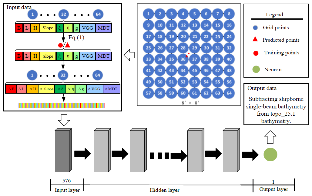
The training dataset includes all shipborne single-beam bathymetric point within the global ocean, which are referred to as the training points. The input data used for training/prediction in this paper are the differences between the multi-source marine geodetic data of training/prediction points and their surrounding grid points, which include the location information (longitude, latitude), bathymetry, slope, meridional components of vertical deflection, prime components of vertical deflection, vertical gravity gradient, gravity anomaly and MDT data. As the ratio of depth difference to distance, slope contains information about the undulating variations of seafloor topography. Therefore, slope is also used as input data in this paper. The relevant calculation equation is as follows:

$$\begin{array}{}\text{(2)}& \left\{\begin{array}{ll}\mathrm{\Delta }L=L_{\mathrm{grid}}^i-L_{\mathrm{s}}& \\ \mathrm{\Delta }B=B_{\mathrm{grid}}^i-B_{\mathrm{s}}& \\ \mathrm{\Delta }h=h_{\mathrm{grid}}^i-h_{\mathrm{s}}& \\ \mathrm{\Delta }\mathrm{slope}={\mathrm{slope}}_{\mathrm{grid}}^i-{\mathrm{slope}}_{\mathrm{s}}& \\ \mathrm{\Delta }\mathit{\xi }={\mathit{\xi }}_{\mathrm{grid}}^i-{\mathit{\xi }}_{\mathrm{s}},& i=\mathrm{1},\mathrm{2},\mathrm{\dots },\mathrm{64},\\ \mathrm{\Delta }\mathit{\eta }={\mathit{\eta }}_{\mathrm{grid}}^i-{\mathit{\eta }}_{\mathrm{s}}& \\ \mathrm{\Delta }\left(\mathrm{\Delta }g\right)=\mathrm{\Delta }{g}_{\mathrm{grid}}^i-\mathrm{\Delta }{g}_{\mathrm{s}}& \\ \mathrm{\Delta }\mathrm{VGG}={\mathrm{VGG}}_{\mathrm{grid}}^i-{\mathrm{VGG}}_{\mathrm{s}}& \\ \mathrm{\Delta }\mathrm{MDT}={\mathrm{MDT}}_{\mathrm{grid}}^i-{\mathrm{MDT}}_{\mathrm{s}}& \end{array}\right.\end{array}$$

where i represents the ith grid node; $L_{\mathrm{grid}}^i$ and $B_{\mathrm{grid}}^i$ are the longitude and latitude at the ith grid node; L_s and B_s represent the longitude and latitude at the training or prediction point; $h_{\mathrm{grid}}^i$, ${\mathit{\xi }}_{\mathrm{grid}}^i$, ${\mathit{\eta }}_{\mathrm{grid}}^i$, $\mathrm{\Delta }{g}_{\mathrm{grid}}^i$, ${\mathrm{VGG}}_{\mathrm{grid}}^i$ and ${\mathrm{MDT}}_{\mathrm{grid}}^i$ represent the interpolations of the topo_25.1 model, the SIO meridional components of vertical deflection model, the SIO prime components of vertical deflection model, the SDUST2022GRA gravity anomaly model, the SIO vertical gravity gradient model and the MDT model at the ith grid node; and h_s, ξ_s, η_s, Δg_s, VGG_s and MDT_s represent the interpolations of the topo_25.1 model, the SIO meridional components of vertical deflection model, the SIO prime components of vertical deflection model, the SDUST2022GRA gravity anomaly model, the SIO vertical gravity gradient model and the MDT model at the training or prediction point. The slope, defined as the ratio of the difference in seafloor height to distance, is calculated by the following equation:

$$\begin{array}{}\text{(3)}& {\mathrm{slope}}_i={\displaystyle \frac{h_i-h_{i+\mathrm{1}}}{\sqrt{(x_i-x_{i+\mathrm{1}}{)}^{\mathrm{2}}+(y_i-y_{i+\mathrm{1}}{)}^{\mathrm{2}}}}},\end{array}$$

where slope_i represents the slope of the target point at the ith location; h_i is the bathymetry at the ith point; and h_i+1 is the bathymetry at the i+1th point, which is 1^′ longitudinally or latitudinally apart from the ith point. x_i and y_i are the horizontal and vertical coordinates of the ith point, and x_i+1 and y_i+1 are the corresponding coordinates of the i+1th point. Using Eq. (3), the slopes in four directions – longitudinal and latitudinal – are calculated. The maximum value among these four directional slopes is taken as the final slope for the target point.

The output data used for training are

$$\begin{array}{}\text{(4)}& \mathrm{\Delta }{h}_{\mathrm{output}}=h_{\mathrm{topo}}-h_{\mathrm{s}},\end{array}$$

where Δh_output represents the output data, h_topo represents the bathymetry of the topo_25.1 model at training point and h_s represents the measured bathymetry at the training point.

Table 1 Training accuracy of each sub_region.

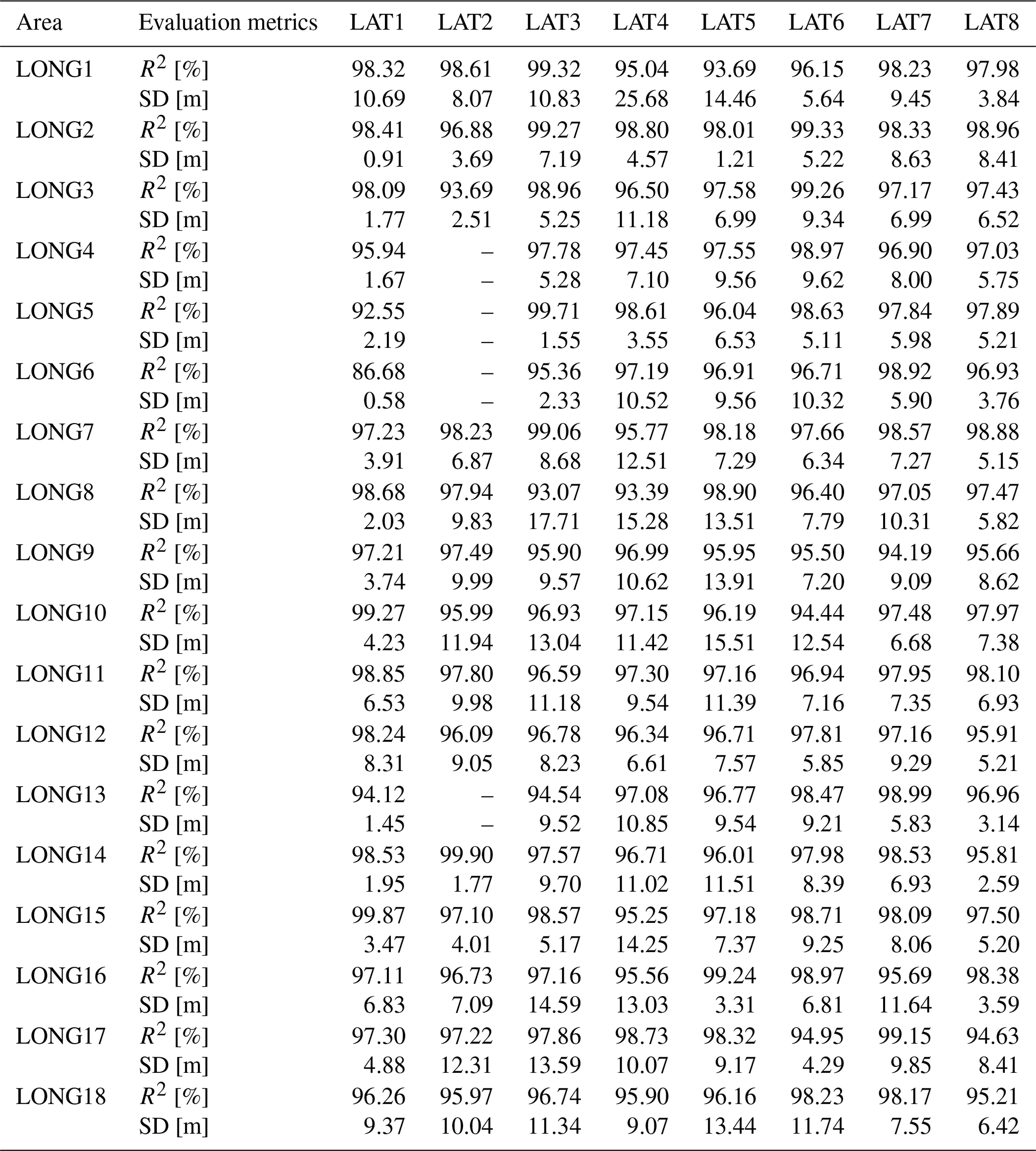
Note: The dash (–) indicates that the area is land or does not have shipboard bathymetric soundings.

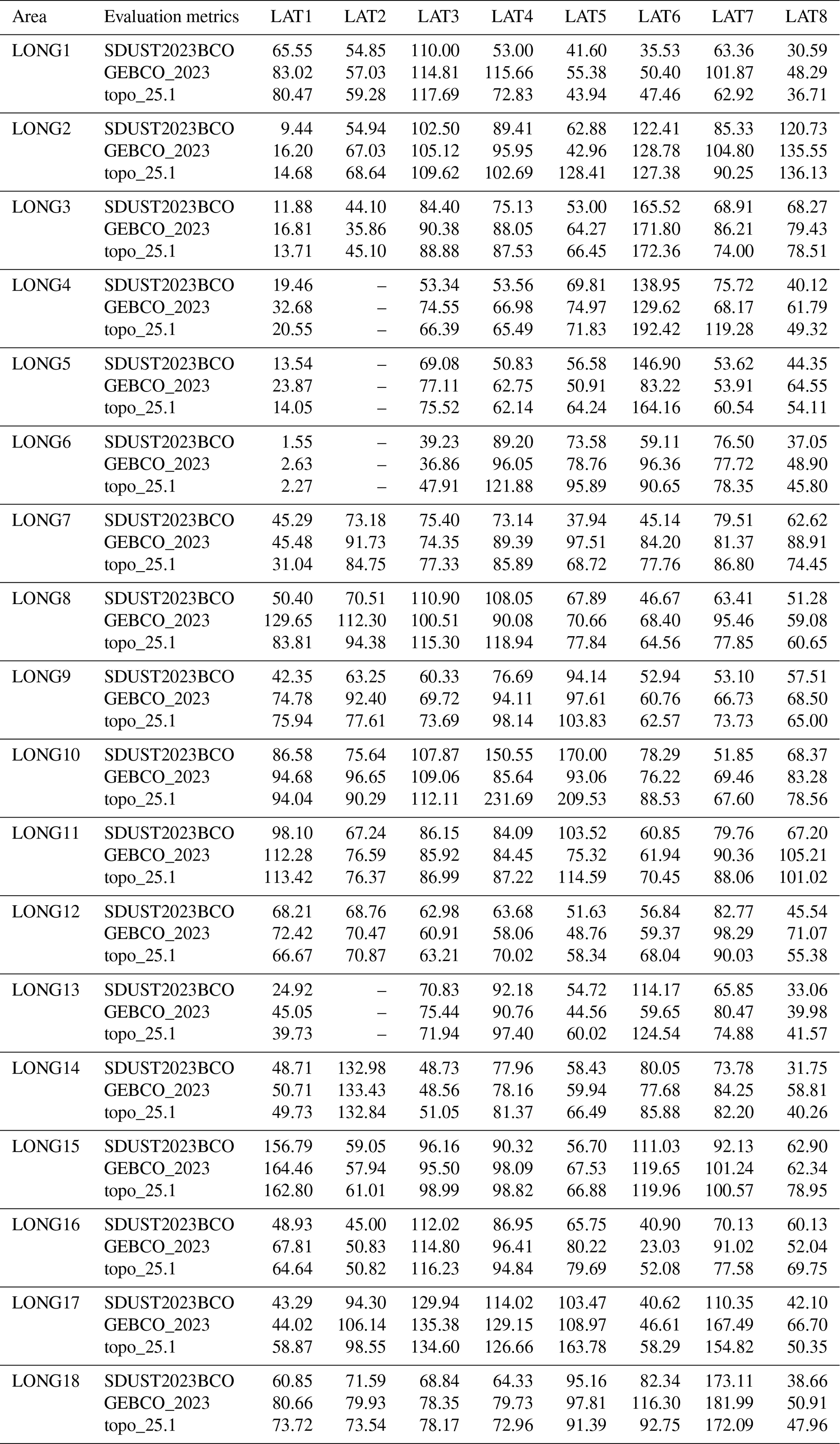
Table 2 RMSE of differences between bathymetric model and shipborne single-beam bathymetric data (in m).

3.3 Method for model construction

The procedure for constructing a global marine bathymetric model using an MLP neural network is illustrated in Algorithm 1, with the specific steps detailed as follows.

The first step is the standardization of the input and output data. Due to the significant differences in magnitude among various types of data, it is essential to standardize both input and output data to mitigate the effects of dimensional discrepancies. The calculation equation is as follows:

$$\begin{array}{}\text{(5)}& \widehat{x}={\displaystyle \frac{x_i-\stackrel{\mathrm{‾}}{x}}{\mathit{\sigma }}},\end{array}$$

where $\widehat{x}$ represents the standardized data, x_i is the data before standardization, $\stackrel{\mathrm{‾}}{x}$ is the mean of the input data and σ is the SD of the input data. After standardization, the mean of the input data becomes 0 and the SD becomes 1, ensuring that all input data contribute equally to the training of the MLP neural network.

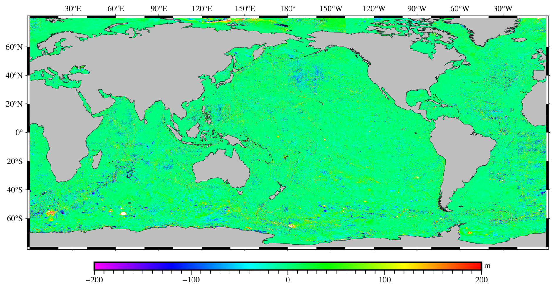
Figure 3 Difference in seafloor topography between the SDUST2023BCO model and the topo_25.1 model.

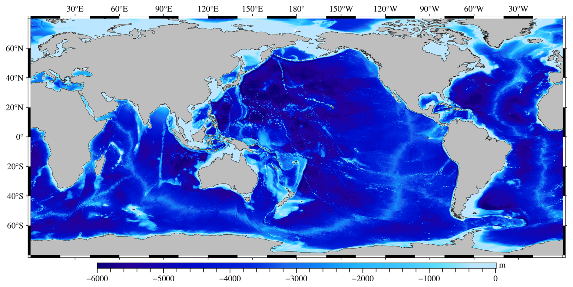
Figure 4 The SDUST2023BCO model.

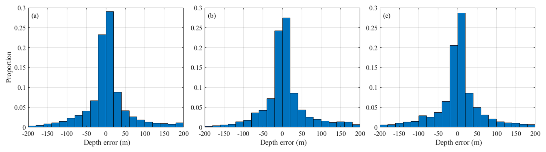
Figure 5 Distribution histogram of the difference between SDUST2023BCO, topo_25.1 and GEBCO_2023 models and shipborne single-beam bathymetric data: (a) SDUST2023BCO, (b) GEBCO_2023 and (c) topo_25.1.

The second step is to select appropriate neural network parameters. The choice of parameters is critical for the training and prediction accuracy of the MLP model. This includes the initialization of weights and biases, number of hidden layers, activation function, learning rate and batch size. In order to achieve high precision in training and prediction, the selection of parameters may be adjusted in different sub-regions. Relevant parameters are initially set randomly, and individual parameters are then adjusted based on training accuracy until the most suitable parameters are obtained. For example, if the training accuracy is poor, increasing the number of hidden layers, the number of neurons in each hidden layer or the number of iterations or decreasing the learning rate or batch size can help achieve the most appropriate parameters. The relevant hyperparameters were determined through the training set and validation set. In this paper, a four-layer hidden neural network is used, with each layer containing 512, 256, 128 and 64 neurons, respectively. The learning rate is set to 0.0001, and the batch size is set to 8.

The third step is the training of the MLP model. First, the MLP neural network is trained using the input and output data. Second, an appropriate loss function and optimization algorithm should be selected. Finally, the MLP neural network models for 144 sub-regions are established through training. In this paper, the mean squared error (MSE) is chosen as the loss function, and the Adam optimization algorithm is used to update the weight and bias.

The fourth step is the calculation of bathymetric values. Based on step 3, 144 MLP neural network models for the sub-regions are established. The prediction outcomes for each sub-region are obtained by feeding the input data into the corresponding MLP models for all 144 sub-regions. Since the prediction result is the difference between the topo_25.1 model at the prediction points and the actual bathymetric value at these points, the equation for calculating the predicted bathymetry value is

$$\begin{array}{}\text{(6)}& h_{\mathrm{output}}^{\mathrm{pred}}=h_{\text{topo\_25.1}}^{\prime }-\mathrm{\Delta }{h}_{\mathrm{result}}^{\prime },\end{array}$$

where $h_{\mathrm{output}}^{\mathrm{pred}}$ represents the predicted bathymetric value at the prediction point, $\mathrm{\Delta }{h}_{\mathrm{result}}^{\prime }$ represents the prediction output result of the MLP model and $h_{\text{topo\_25.1}}^{\prime }$ represents the bathymetric interpolation from the topo_25.1 model at the prediction point.

The final step is the construction of the global bathymetric model. Due to each sub-region being extended outward by 0.1°, the average bathymetry of the overlapping areas is taken as the final bathymetric value. This method ensures a smooth transition between sub-regions and avoids any abrupt changes in the bathymetric model. By integrating all sub-regions, a new global bathymetric model is constructed.

Algorithm 1 MLP neural network for constructing the seafloor topography model.

1:

Input: training set T and prediction set P for each sub-region.

2:

Initialization: normalize the datasets using the Eq. (5); N denotes the number of iterations.

3:

for i =  1 to N do

4:

Initialize the weight W and bias b values.

5:

Compute the output of each neuron in each layer and the final output using Eq. (1).

6:

Calculate the loss function.

7:

Update the weight W and bias b values using the Adam algorithm.

8:

end for

9:

until the maximum number of iterations is reached or the loss function no longer decreases;

10:

Save the MLP model.

11:

Obtain prediction values using the prediction set P.

12:

Recover the bathymetry values using Eq. (6).

13:

Bathymetry models for each sub-region.

14:

Output: Global bathymetry model.

4 Results and analysis

4.1 Training results of the MLP neural network

First, input and output data are organized according the Sect. 3.2. Second, the MLP neural network is trained with those data to establish MLP models for each sub-region. Through the training phase, the weights within the MLP neural network are iteratively adjusted via the Adam optimization algorithm. The training outcomes gradually converge to the actual bathymetric values, and the MLP models for each sub-region are constructed.

Table 3 Difference in statistical results between SDUST2023BCO, GEBCO_2023 and topo_25.1 models and shipborne single-beam bathymetric points (in m).

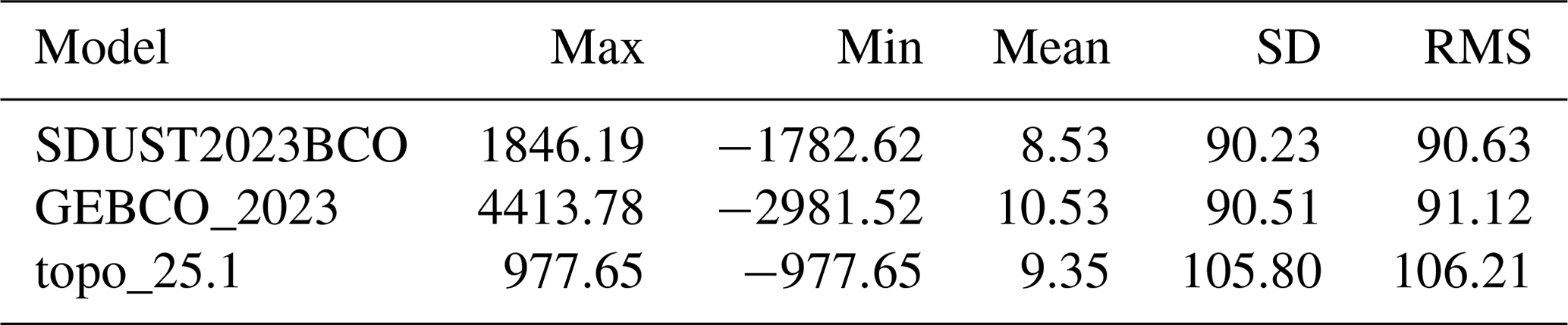
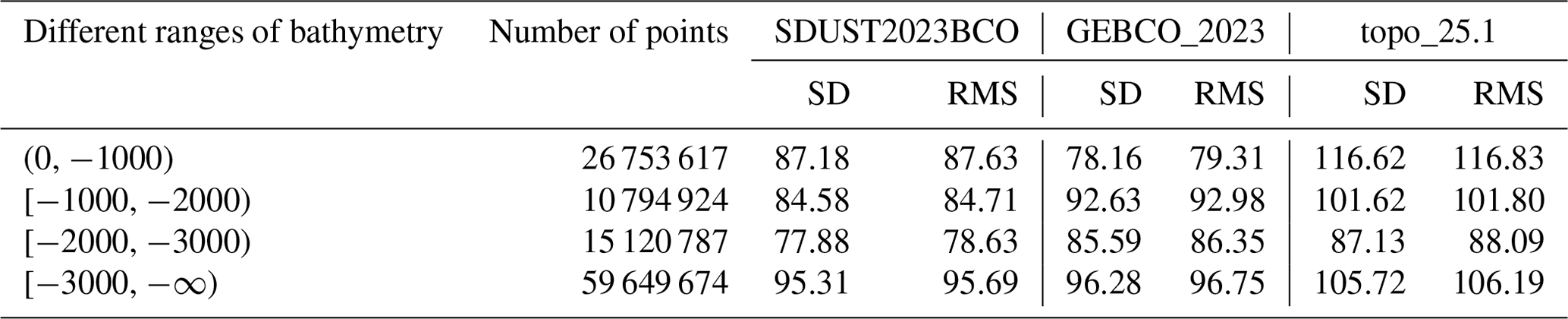
Table 4 Statistical results of the difference between SDUST2023BCO, GEBCO_2023 and topo_25.1 models and the measured bathymetry at shipborne single-beam bathymetric points in different ranges of bathymetry (in m).

In order to evaluate the training accuracy of the MLP neural network, and the coefficient of determination (R²) is introduced, the calculation equation is as follows:

$$\begin{array}{}\text{(7)}& R^{\mathrm{2}}=\left(\mathrm{1}-{\displaystyle \frac{\left(\sum _{i=\mathrm{1}}^n(h_i^{\mathrm{pred}}-h_i{)}^{\mathrm{2}}\right)}{\sum _{i=\mathrm{1}}^n(\stackrel{\mathrm{‾}}{h}-h_i{)}^{\mathrm{2}}}}\right)\times \mathrm{100}\mathit{\%},\end{array}$$

where $h_i^{\mathrm{pred}}$ is the predicted bathymetry of the ith training point, h_i is the measured bathymetry of the ith training point, $\stackrel{\mathrm{‾}}{h}$ is the average value of the measured bathymetry of the training point and n is the number of training points. R² is generally used to indicate the accuracy of training, and the greater it is, the better it is.

Table 1 shows the training accuracy for each sub-region, which indicates that approximately 91.4 % of the sub-regions achieve a training accuracy exceeding 95 %. This indicates that the MLP models constructed for these sub-regions have achieved a high level of accuracy. This satisfies the requirements for predicting bathymetry, demonstrating the effectiveness of these models for this application.

4.2 SDUST2023BCO model based on MLP neural network

Input data at the prediction points within each sub-region are fed into the respective MLP model, the predicted bathymetry for the center points of each 1^′ × 1^′ grid are obtained. The predicted bathymetry is the difference between the STUST2023BCO model and the topo_25.1 model. Figure 3 presents the difference map between the two models, illustrating that the discrepancies are mainly centered around 0 m. According to statistics, the ratio of differences that fall within the range of ±100 m is 96.89 %. The high correlation and minimal differences between the two models, as revealed by this analysis, further validate the effectiveness of the MLP neural network method in constructing bathymetric models.

Using Eq. (6), the predicted bathymetry for each sub-region is obtained. In the overlapping areas of the sub-regions, the final bathymetric value is obtained by averaging the values from these regions. Finally, the STUST2023BCO model is constructed using this method, as shown in Fig. 4.

4.3 Comparison with NCEI shipborne single-beam bathymetric points

The distribution of shipborne single-beam bathymetric points is showed in Fig. 1. In order to verify the similarity between the SDUST2023BCO, GEBCO_2023 and topo_25.1 models and shipborne single-beam bathymetric data, the RMS of the differences between the shipborne single-beam bathymetric data and the three global marine bathymetric models is calculated within each sub-region, as shown in Table 2.

Table 5 Statistical results of the bathymetry of SDUST2023BCO, GEBCO_2023 and topo_25.1 models (in m).

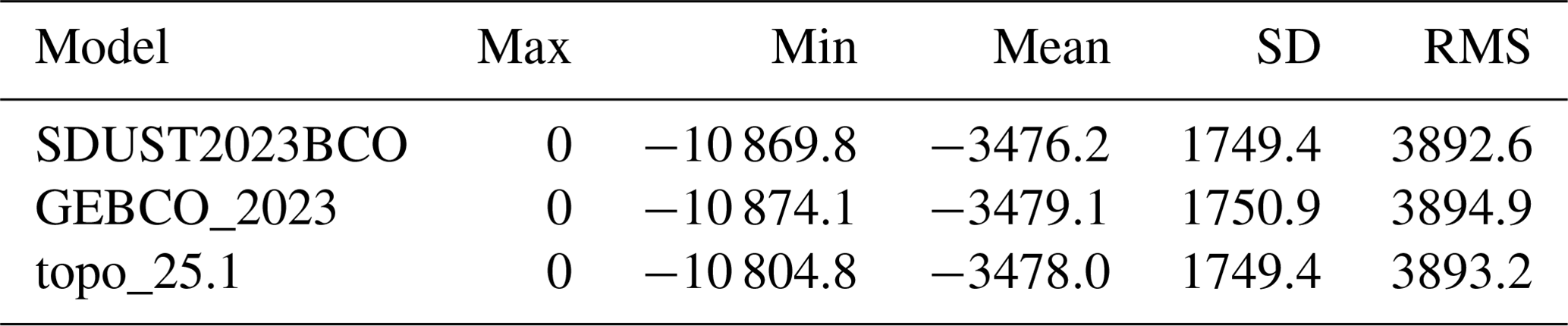
Table 6 Statistical results of differences between SDUST2023BCO, GEBCO_2023 and topo_25.1 models (in m).

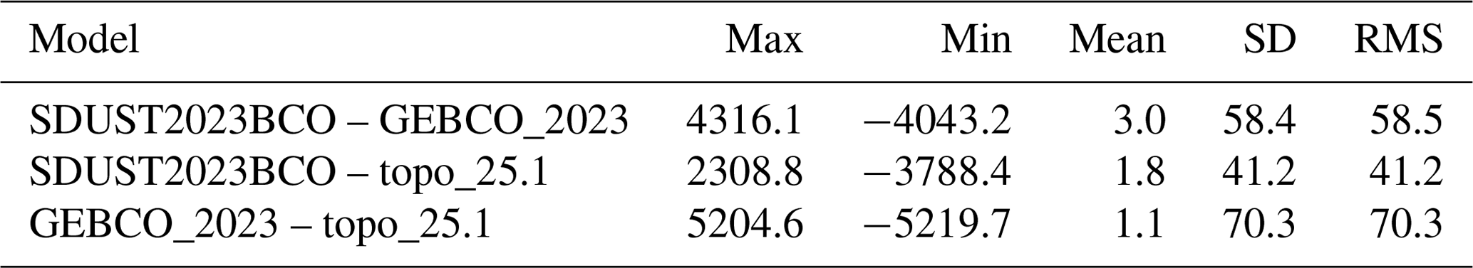
Table 2 shows that the SDUST2023BCO, topo_25.1 and GEBCO_2023 models have their strengths and weaknesses in different sub-regions. The results indicate that the SDUST2023BCO model shows closer resemblance to shipborne single-beam bathymetric data in 112 and 134 sub-regions compared to the GEBCO_2023 model and the topo_25.1 model, respectively, which corresponds to approximately 80.00 % and 95.71 % of the total number of sub-regions. In conclusion, the SDUST2023BCO model is more closely aligned with the shipborne single-beam bathymetric data.

To validate the reliability of the SDUST2023BCO model, each model is interpolated onto all shipborne single-beam bathymetric points using a cubic spline interpolation method, the relevant statistical results are showed in Table 3. Table 3 shows that the models, ranked from closest to furthest resemblance to the shipborne single-beam bathymetric data, are the SDUST2023BCO model, followed by the GEBCO_2023 model, and the topo_25.1 model. Compared to the GEBCO_2023 and topo_25.1 models, the SD of the SDUST2023BCO model is improved by 0.28 and 15.57 m, respectively. The statistical results show that the SDUST2023BCO model exhibits superior reliability compared to the GEBCO_2023 and topo_25.1 models, aligning more closely with the shipborne single-beam bathymetric data.

Figure 5 shows the histogram distribution of the differences between the SDUST2023BCO, GEBCO_2023 and topo_25.1 models and the shipborne single-beam bathymetric data, showing that the error distributions of all three models exhibit a normal distribution. The percentages of differences between the bathymetric models and the actual bathymetry falling within the ±50 m range are 72.44 %, 72.01 % and 68.92 %, respectively. The distribution of differences between the SDUST2023BCO model and the shipborne single-beam bathymetric data are more concentrated, demonstrating a superior reliability to reflect the information of the seafloor topography.

Table 4 presents the statistical results of the comparison between the SDUST2023BCO, GEBCO_2023 and topo_25.1 models and shipborne single-beam bathymetric data at different depths. The reliability of the SDUST2023BCO model outperforms the GEBCO_2023 and topo_25.1 models across depth intervals of −1000 to −2000 m, −2000 to −3000 m and below −3000 m, with improvements of 8.05 and 17.04 m, 7.71 and 9.25 m, and 0.97 and 10.41 m, respectively. In waters shallower than 1000 m, the GEBCO_2023 model shows closer proximity to the shipborne bathymetric points compared to the topo_25.1 and SDUST2023BCO models. Overall, the SDUST2023BCO model exhibits commendable reliability in deeper waters.

4.4 Comparison with SIO topo_25.1 and GEBCO_2023

To verify the accuracy of the SDUST2023BCO model, the bathymetric information for the SDUST2023BCO, GEBCO_2023 and topo_25.1 models are calculated, as shown in Table 5.

Table 5 shows that the SD of SDUST2023BCO model is 1749.4 m, differing by 1.5 and 0.0 m from the GEBCO_2023 and topo_25.1 models, respectively. Additionally, the minimum and mean values of SDUST2023BCO model are closely aligned with those of GEBCO_2023 and topo_25.1 models. Considering all these indicators, the consistency of the SDUST2023BCO model with the GEBCO_2023 and topo_25.1 models is effectively validated.

To further validate the consistency of the SDUST2023BCO model with other models, the differences between the SDUST2023BCO, GEBCO_2023 and topo_25.1 models are calculated. Relevant statistical outcomes are showed in Table 6. Owing to the SDUST2023BCO model having a resolution of 1^′ × 1^′, the bathymetric values at 1^′ grid nodes are selected from the GEBCO_2023 model, and the GEBCO_2023 model is processed into a bathymetric model with a resolution of 1^′.

Table 6 shows that the SD of the differences between the SDUST2023BCO model and the other models is 58.4 and 41.2 m, respectively. This indicates that the SDUST2023BCO model has the highest correlation with the topo_25.1 model, followed by the GEBCO_2023 model. The SDUST2023BCO model shows commendable consistency with the GEBCO_2023 and topo_25.1 models, demonstrating the reliability and effectiveness of this method.

Figure 6 shows the histogram distributions of the differences between the three bathymetric models. From Fig. 6a, we see that the differences between the SDUST2023BCO and GEBCO_2023 models are mainly within the range of −100 to 100 m, accounting for approximately 94.51 %. From Fig. 6b, we can conclude that the differences between the SDUST2023BCO and topo_25.1 models within the same range account for about 96.89 %. From Fig. 6c, it is evident that the differences between the topo_25.1 model and the GEBCO_2023 model within the range of −100 to 100 m account for approximately 93.38 %. Based on the above statistics, the SDUST2023BCO model exhibits commendable consistency with the GEBCO_2023 and topo_25.1 models.

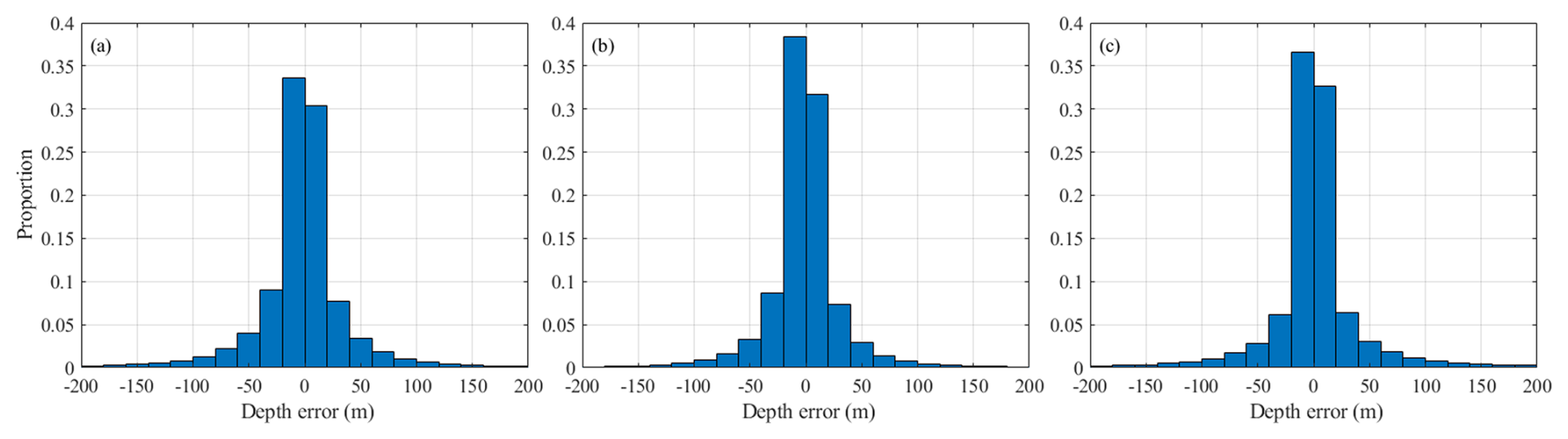
Figure 6 Histogram of the difference between the SDUST2023BCO, topo_25.1 and GEBCO_2023 models: (a) SDUST2023BCO − GEBCO_2023, (b) SDUST2023BCO − topo_25.1 and (c) GEBCO_2023 − topo_25.1.

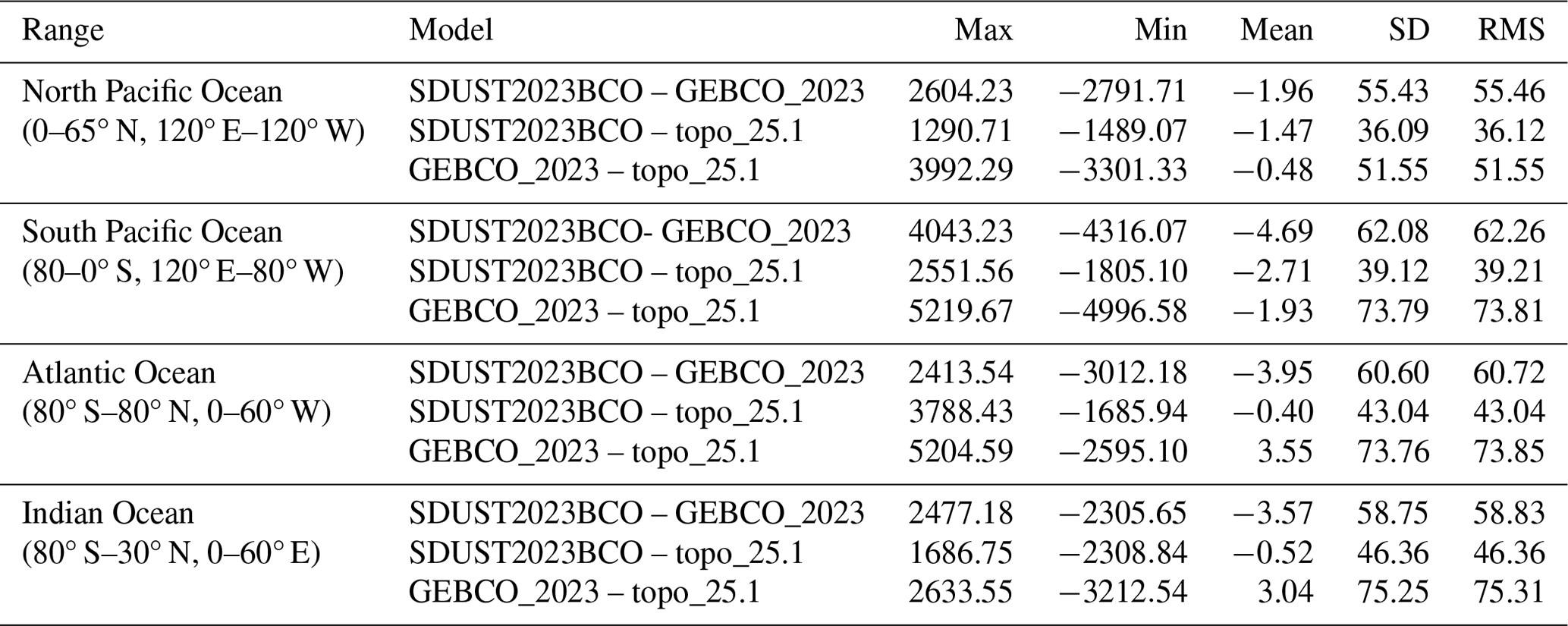
Table 7 Statistical results of the differences between the SDUST2023BCO and GEBCO_2023 and topo_25.1 models within various regions (in m).

According to the law of error propagation, assuming that the SDUST2023BCO, GEBCO_2023 and topo_25.1 models are uncorrelated, the SD of these three models can be expressed as

$$\begin{array}{}\text{(8)}& \left\{\begin{array}{l}{\mathrm{SD}}_{\text{S\_G}}^{\mathrm{2}}={\mathrm{SD}}_{\mathrm{S}}^{\mathrm{2}}+{\mathrm{SD}}_{\mathrm{G}}^{\mathrm{2}},\\ {\mathrm{SD}}_{\text{S\_t}}^{\mathrm{2}}={\mathrm{SD}}_{\mathrm{S}}^{\mathrm{2}}+{\mathrm{SD}}_{\mathrm{t}}^{\mathrm{2}},\\ {\mathrm{SD}}_{\text{G\_t}}^{\mathrm{2}}={\mathrm{SD}}_{\mathrm{G}}^{\mathrm{2}}+{\mathrm{SD}}_{\mathrm{t}}^{\mathrm{2}},\end{array}\right.\end{array}$$

where SD_{S_G}, SD_{S_t} and SD_{G_t}, respectively, represent the SD of comparisons between the SDUST2023BCO and GEBCO_2023 models, the SDUST2023BCO and topo_25.1 models, and the GEBCO_2023 and topo_25.1 models. SD_S, SD_G and SD_t, respectively, represent the SD of the bathymetric values of the SDUST2023BCO, GEBCO_2023 and topo_25.1 models.

Using Eq. (8) and the statistical results in Table 6, the SD_S, SD_G and SD_t can be calculated to be 9.11, 57.69 and 40.18 m, respectively. The high correlation between SDUST2023BCO model and topo_25.1 model causes the value of SD_S to be small. This result indicates that the accuracy of the three models, from highest to lowest, is the SDUST2023BCO, topo_25.1 and GEBCO_2023 models. This effectively demonstrates that the SDUST2023BCO model has better reliability among the three models.

Furthermore, four regions are selected to validate the reliability of bathymetric model, specifically the North Pacific Ocean (0–65° N, 120° E–120° W), the South Pacific Ocean (80–0° S, 120° E–80° W), the Atlantic Ocean (80° S–80° N, 0–60° W) and the Indian Ocean (80° S–30° N, 0–60° E). Relevant statistical results are showed in Table 7. Table 7 shows that the SDUST2023BCO model exhibits better reliability across all regions, further substantiating its reliability in the various oceans.

5 Data availability

The global bathymetric model (SDUST2023BCO) can be downloaded from https://doi.org/10.5281/zenodo.13341896 (Zhou et al., 2024). The dataset includes geospatial information (latitude, longitude) and corresponding bathymetric values.

6 Conclusion

Considering the effectiveness in the construction of bathymetric models, the influence of long-wavelength information derived from multi-source geodetic datasets, and the nonlinear interrelation between multi-source marine geodetic data and bathymetry, a new global marine model, designated the SDUST2023BCO model, has been constructed. This model has a resolution of 1^′ × 1^′, with spatial coverage ranging from 0 to 360° E in longitude and from 80° S to 80° N in latitude. This model is constructed based on the MLP neural network using the differences from multi-source marine geodetic data. The reliability of the SDUST2023BCO model has been evaluated by shipborne single-beam bathymetric data, as well as the GEBCO_2023 and topo_25.1 models.

Compared to the shipborne single-beam bathymetric data, the SDUST2023BCO model achieves an SD of 90.23 m, which is superior to other bathymetric models, demonstrating the reliability of the SDUST2023BCO model. Through the comparison of the accuracy of three models in different depth, the SDUST2023BCO model demonstrates superior reliability in deeper water regions.

The discrepancies between the SDUST2023BCO model and the GEBCO_2023 and topo_25.1 models primarily fall within ±100 m, confirming the consistency of the SDUST2023BCO model with existing models. This paper also evaluates the accuracy of the SDUST2023BCO model in four distinct regions across the Pacific, Atlantic and Indian oceans, effectively validating its reliability.

The results presented in this paper demonstrate that SDUST2023BCO reaches an international advanced level of global bathymetric models. The accuracy of the SDUST2023BCO model is better than that of GEBCO_2023 and topo_25.1 models, especially in deeper water regions.