The International Altimetry Service 2024 (IAS2024) coastal sea level dataset and first evaluations

A new dedicated 20 Hz coastal sea level dataset, called the International Altimetry Service 2024 (IAS2024, https://doi.org/10.5281/zenodo.13208305, Peng et al., 2024c), is presented for monitoring sea level changes along the world's coastlines. One of the reasons for generating this dataset is that the quality of coastal altimeter data has been greatly improved with advanced coastal reprocessing strategies. In this study, the Seamless Combination of Multiple Retrackers (SCMR) strategy is adopted to obtain the reprocessed Jason data from January 2002 to April 2022. The evaluation/validation results show that the IAS2024 20 Hz along-track coastal sea level dataset achieves good performance over global coastal oceans. The good consistency between IAS2024 and independent altimeter datasets, including the European Space Agency Climate Change Initiative version 2.4 (ESA CCI v2.4) 20 Hz along-track coastal sea level dataset and the Copernicus Marine Environment Monitoring Service Level-3 (CMEMS L3) 1 Hz along-track sea level dataset, is observed. The closure of sea level trend differences (0.16 ± 3.97 mm yr⁻¹) between IAS2024 and Permanent Service for Mean Sea Level (PSMSL) tide gauge data at the global scale is also achieved. Moreover, 1548 virtual stations have been constructed using the IAS2024 coastal sea level dataset, which will contribute to the analysis of coastal sea levels for the ocean community and to risk management for the policymakers. Our study also finds that no obvious variations exist in the linear sea level trends from the offshore to the coast over the last 20 km coastal strip at the global scale. In addition, the vertical land motion (VLM) estimates from the combination of the IAS2024 dataset with the PSMSL tide gauge records agree well with the University of La Rochelle 7a (ULR7a) Global Navigation Satellite System (GNSS) solution, with the mean difference of VLM estimates being 0.12 ± 2.27 mm yr⁻¹, suggesting that altimeter-derived VLM estimates can be used as an independent data source to validate the GNSS solutions.

1 Introduction

Satellite altimetry has become a mature remote sensing technique over open oceans since the launch of high-precision satellite altimetry missions (e.g., Topex and Poseidon). It has been making great contributions to quantifying and monitoring sea level changes at both global and regional scales (Ablain et al., 2017; Prandi et al., 2021; Guérou et al., 2023). Among these missions, the Jason altimetry series are usually used as the reference missions for monitoring global sea levels considering their high-precision and stable performance. During the past 2 decades, the precision of reprocessed 20 Hz along-track altimeter data in coastal zones from Jason missions has been remarkably increased thanks to the dedicated coastal retrackers and improved range/geophysical corrections (Cipollini et al., 2017; Vignudelli et al., 2019; Peng et al., 2024a), which makes it possible to construct altimeter-based virtual stations along the world's coastlines (Benveniste et al., 2020; Cazenave et al., 2022).

The IAS (International Altimetry Service) Pilot Service was established in July 2023 as a service of the International Association of Geodesy (IAG) for providing information about altimetry data, geodetic and climate models, research, and operational applications based on satellite altimetry technology innovations. One of its goals is to provide auxiliary data and algorithms to produce new products across coastal zones, including the coastal oceans, land–sea surfaces, estuaries and inland waterbodies for applications in studies of the extremes, long-term climate change and environmental development.

In this paper, we present the IAS2024 20 Hz along-track coastal sea level dataset from Jason missions over the period of January 2002 and April 2022 reprocessed with the SCMR (Seamless Combination of Multiple Retrackers) strategy. A total of 1548 virtual stations are built along the world's coastlines, which can be used to monitor the coastal sea levels and estimate the vertical land motions (VLMs). In addition, the spatial variation of 20 Hz along-track sea level trends from the offshore to nearshore in the last 20 km to the coast is analyzed using the IAS2024 dataset. The quality of reprocessed altimeter data is validated against the monthly tide gauge records from the PSMSL (Permanent Service for Mean Sea Level, https://psmsl.org/, last access: 29 September 2024), the Copernicus Marine Environment Monitoring Service (CMEMS) L3 1 Hz along-track product (https://data.marine.copernicus.eu/product/SEALEVEL_GLO_PHY_L3_MY_008_062/description, last access: 29 September 2024) and the European Space Agency (ESA) Climate Change Initiative (CCI) version 2.4 20 Hz along-track coastal sea level dataset (https://www.seanoe.org/data/00631/74354/, last access: 5 December 2024).

Section 2 presents the details of the SCMR processing strategy and methods to construct the altimeter-based virtual stations and to assess the quality of reprocessed altimeter data. Sections 3 and 4 illustrate the cross-validation results against in situ and independent altimeter datasets as well as the application of coastal altimeter datasets. Sections 5 and 6 present the data availability and conclusions, respectively.

2 Computation of the IAS2024 coastal sea level dataset

2.1 The SCMR strategy

The IAS2024 coastal sea level dataset is generated using the SCMR (Peng et al., 2024b) strategy. The flow diagram is illustrated in Fig. 1, which starts from the waveform leading-edge detection and ends with the seamless combination of sea surface height (SSH) estimates from multiple retrackers. Four different waveform retrackers are used in this study, which are the official Sensor Geophysical Data Record (SGDR) maximum likelihood estimator four-parameter (MLE4) retracker (Amarouche et al., 2004), the Adaptive Leading-Edge Sub-waveform (ALES, Passaro et al., 2014), the weighted least-squares three-parameter (WLS3, Peng and Deng, 2018) and the modified Brown model four-parameter (MB4) retracker (Poisson et al., 2018). The main steps are described in the following subsections.

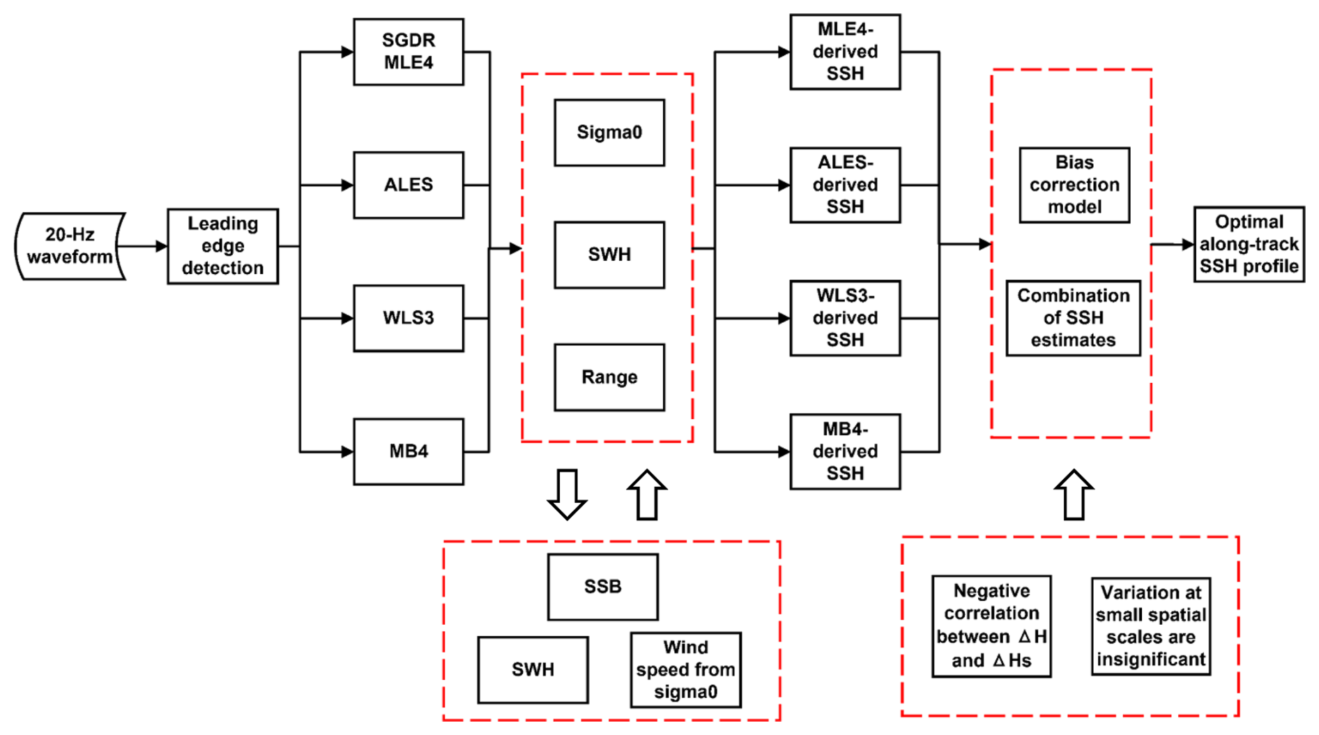
Figure 1 Flow diagram of the SCMR processing strategy. It consists of four operating blocks from left to right: (1) four retrackers of the SGDR MLE4, ALES, WLS3 and MB4; (2) estimating sigma0, SWH and range estimates from different retrackers; (3) calculating SSH estimates for different retrackers; and (4) removing inter-retracker bias and combining SSH estimates from different retrackers. The sea state bias (SSB) corrections are individually computed for each retracker. The inter-retracker bias correction model is developed based on the negative correlation between SSH differences (Δh) and SWH differences (ΔH_s) with respect to the SGDR MLE4 retracker. The combination of SSH estimates from four retrackers is conducted using the Dijkstra (1959) algorithm based on the situation where the altimeter along-track SSH estimates do not change significantly at the spatial scale of ∼ 300 m.

2.1.1 Detection of leading edges

The leading edge is a sequence of waveform gates, where the power increases sharply and thus can be detected based on the differences between consecutive powers of gates. The start gate of the leading edge is deemed the first gate where the power difference between two consecutive gates is positive (Passaro et al., 2014). Similarly, the stop gate of the leading edge is deemed the first gate where the power difference between two consecutive gates is negative (Passaro et al., 2014) or smaller than a tiny positive number (Wang et al., 2019). Moreover, the power of the start gate should be lower than a constant level, and the power difference between start and stop gates should be larger than a threshold value (Gommenginger et al., 2011). The main steps of the leading-edge detection method are as follows.

First, the intersection points between four horizontal lines with power levels of 0.1, 0.2, 0.5 and 0.9 and the normalized waveform are derived. For each intersection point, the start and stop gates of the leading edge are searched forward and backward until the following equations are satisfied:

$$\begin{array}{}\text{(1)}& P_{\mathrm{startgate}}-P_{\mathrm{startgate}-\mathrm{1}}>\mathrm{0.001},\end{array}$$

$$P_{\mathrm{stopgate}+\mathrm{1}}-P_{\mathrm{stopgate}}<\mathrm{0.01},$$

where P_startgate and P_stopgate are the powers of the normalized waveform at the start and stop gates. If the difference (i.e., P_stopgate−P_startgate) is larger than 0.1 and the P_startgate is lower than 0.2, the proportion of waveform from start to stop gates is selected as a potential leading edge. Here, the above threshold levels are selected based on previous studies and our empirical experience (Passaro et al., 2014; Peng and Deng, 2020a).

Second, once all potential leading edges are found, the 50 % threshold retracker (Gommenginger et al., 2011) is applied to each potential leading edge to calculate the range and corresponding SSH estimates. The Dijkstra (1959) algorithm is then applied to find the shortest path between the offshore and nearshore along-track points, in which the edge weights are the height differences between connected nodes (Roscher et al., 2017). As a result, the optimal 20 Hz along-track SSH profile and the corresponding leading edge are determined (Peng et al., 2023). The advantage of this method is that it effectively avoids the perturbations before the true leading edge of the waveform (cf. Fig. 2 in Peng et al., 2024b).

2.1.2 Detection of land returns

When the altimeter approaches the coast, the contaminated waveforms appear with peaks that are caused by the high reflective areas inside the illuminated land surfaces or by the modification of the sea state close to the shoreline (Halimi et al., 2013). This type of waveform is denoted as the Brown-peaky waveform because the peaks caused by land returns are close to the waveform leading edge and the waveform shape over oceans follows the Brown model (Fig. 4.5 in Gommenginger et al., 2011). Here, we detect the land returns following the idea of the adaptive peak detection (APD) method (Peng and Deng, 2018, 2020a) shown in Fig. 2 but with some modifications. The main steps are as follows.

Firstly, the forward moving average (F_t) and backward moving average (B_t) are derived using the following normalized waveform:

$$\begin{array}{}\text{(2)}& F_t\left(i\right)={\displaystyle \frac{\mathrm{1}}{N}}\sum _{j=\mathrm{0}}^{N-\mathrm{1}}{P}_t\left(i+j\right),i=\mathrm{1},\mathrm{2},\mathrm{\dots },n-N+\mathrm{1},\end{array}$$

$$B_t\left(i\right)={\displaystyle \frac{\mathrm{1}}{N}}\sum _{j=\mathrm{0}}^{N-\mathrm{1}}{P}_t\left(i-j\right),i=N,N+\mathrm{1},\mathrm{\dots },n,$$

where the N is the moving average step, which is selected to be 5 through our trial-and-error test, and n is the number of waveform gates, which is 104 for Jason missions.

Next, we define the Difference I as (F_t−B_t). This is first used to determine the Leftfoot points, which correspond to the local maxima of Difference I whose height and prominence are larger than 0.12 using the MATLAB function findpeaks. This is then used to determine the Leftedge, Rightfoot and Rightedge points. The Leftedge and Rightedge points are the zero-crossing points of Difference I before and after the corresponding Leftfoot points. The Rightfoot points are the local minima between consecutive Leftfoot points (Fig. 2). If there exist multiple Leftfoot points, the waveform is denoted as the multi-peak waveform (Fig. 2a and b). Otherwise, the waveform is classified as a Brown-peaky waveform if the Difference I of the Rightfoot point is smaller than −0.2 (Fig. 2c and d).

Finally, the start gate of land returns is defined as the stop gate of the leading edge, while the stop gate of land returns is the last zero-crossing point between Rightfoot and Rightedge points (black line in Fig. 2d). Note that the modified APD method used here is dedicated to the Brown-peaky waveforms instead of the multi-peak waveforms.

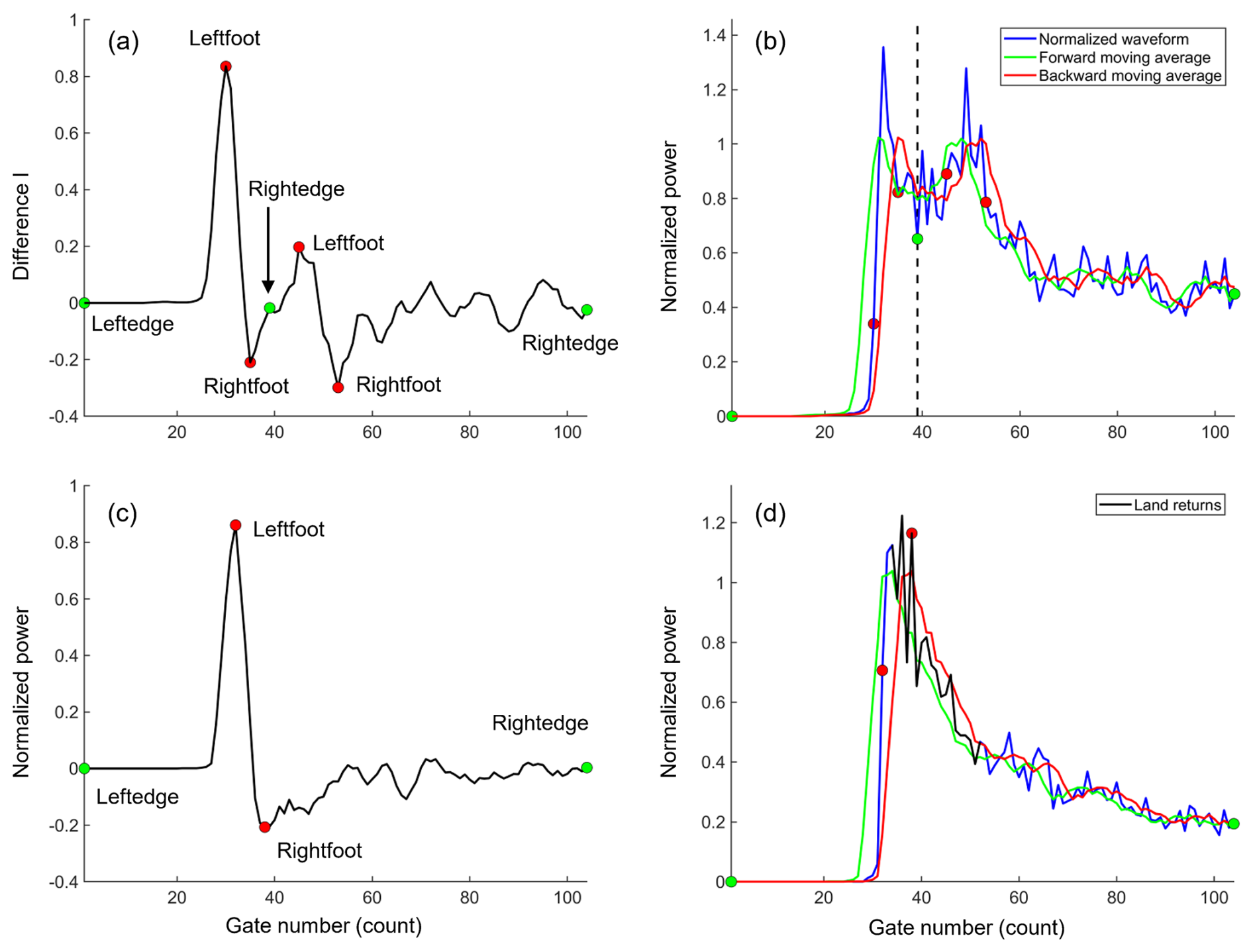
Figure 2 Illustration of the adaptive peak detection (APD) method. Panels (a) and (b) show the curve of Difference I and feature points detected by the APD method for multi-peak waveforms, respectively. Panels (c) and (d) show the similar results for Brown-peaky waveforms. Difference I is calculated as the difference between the forward-moving average and the backward-moving average of the normalized waveform. The black line corresponds to the gates affected by the land returns.

2.1.3 Waveform retracking

All retrackers included in Fig. 1 can process ocean waveforms. Of these, the ALES retracker can handle waveforms with land returns observed in the waveform trailing edge, the WLS3 retracker can cope with the Brown-peaky waveforms with the downsized weights (i.e., 0.01) being assigned to land returns determined by the modified APD method, and the MB4 retracker can deal with the specular waveforms (Fig. 3). Note that the estimates from SGDR MLE4 are directly provided by the official product, while the estimates from the ALES, WLS3 and MB4 retrackers are solved independently.

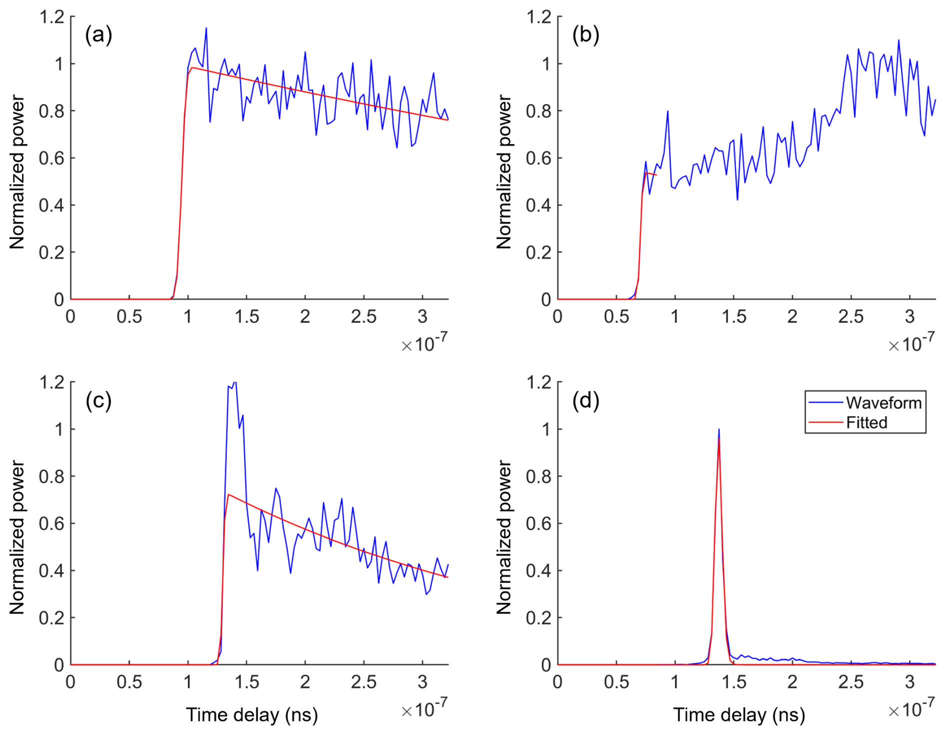
Figure 3 An example of observed waveforms and fitted waveforms from different waveform retrackers. Panels (a)–(d) show the fitted results for different waveform types by methods of (a) SGDR MLE4, (b) ALES, (c) WLS3 and (d) MB4 retrackers.

2.1.4 Calculation of altimeter SSH

The altimeter SSH at each 20 Hz along-track point is calculated as follows:

$$\begin{array}{}\text{(3)}& \mathrm{SSH}=h_{\mathrm{alt}}-R_{\mathrm{r}}-R_{\mathrm{cor}},\end{array}$$

where h_alt is the height of the satellite above the Topex ellipsoid; R_r is the distance between the altimeter and nadir sea surface derived from the waveform retracker; and R_cor includes dry and wet tropospheric, ionospheric, and sea state bias corrections. Note that the Topex ellipsoid is a reference ellipsoid which has an equatorial radius of 6378.1363 km and a flattening coefficient of 1 / 298.257. The appropriate corrections for each altimetry mission are investigated and summarized in Table 1.

Table 1 Range/geophysical corrections applied to Jason missions used in this study.

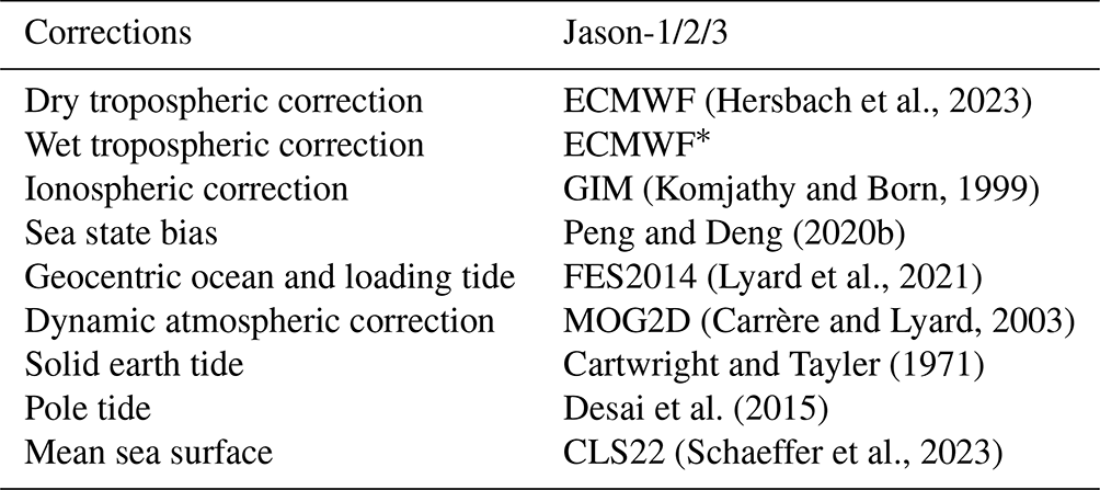
^* The modeled wet tropospheric correction at zero altitude has been used instead of the GNSS-derived Path Delay Plus (GPD+) correction (Fernandes and Lázaro, 2016) considering that the GPD+ is unavailable beyond February 2021. GIM: Global Ionospheric Maps.

2.1.5 Seamless combination of SSH estimates from multiple retrackers

As illustrated by Fig. 1, the coastal retrackers (i.e., ALES, WLS3 and MB4) are applied to all 20 Hz waveforms to derive range estimates, respectively. Combined with satellite altitude, range and geophysical corrections, the SSH estimates for these coastal retrackers and the SGDR MLE4 retracker are obtained. Considering the above retrackers can handle different types of waveforms, as shown in Fig. 3, and achieve similar performance through our previous Monte Carlo simulation (Peng and Deng, 2018; Peng et al., 2021), it is possible to further improve the data availability by combining SSH estimates from these retrackers. However, these retrackers adopt different processing strategies, and there inevitably exist systematic biases between SSH estimates from these retrackers, which prohibit the seamless combination of SSH estimates. To solve this problem, we proposed an inter-retracker bias model to reduce the SSH bias with respect to the SGDR MLE4 from centimeter levels to millimeter levels (Peng et al., 2024b). Finally, the optimal SSH estimate at each along-track point is selected using the Dijkstra (1959) algorithm. The Dijkstra algorithm is used because it can automatically determine the along-track SSH profile with smooth spatial variation (Roscher et al., 2017), which is consistent with the real situation where the altimeter along-track SSH estimates do not change significantly at the spatial scale of ∼ 300 m (Cipollini et al., 2017). Moreover, the Dijkstra algorithm does not rely on the waveform classification results. For more detailed information about the use of the Dijkstra algorithm, readers can refer to Peng et al. (2023).

The analytical form of the inter-retracker bias correction model is as follows (Peng et al., 2024b):

$$\begin{array}{}\text{(4)}& {\displaystyle }\mathrm{\Delta }h=\mathit{\rho }\times \mathrm{\Delta }{H}_{\mathrm{s}}+c_b,\text{(5)}& {\displaystyle }{h}_{\mathrm{cor}}=\widehat{\mathit{\rho }}\times \mathrm{\Delta }{H}_{\mathrm{s}}+\widehat{c_b},\end{array}$$

where ΔH_s and Δh are the significant wave height (SWH) difference and SSH difference with respect to the SGDR MLE4 retracker (e.g., ALES minus SGDR MLE4), and ρ and c_b are the linear regression slope and intercept parameters, which are unknown and need to be estimated. Once the estimates of the two parameters, $\widehat{\mathit{\rho }}$ and $\widehat{c_b}$, are determined, the inter-retracker bias correction, h_cor, can be calculated by substituting SWH difference ΔH_s into Eq. (5). After removing the inter-retracker bias, the most appropriate SSH profile between the offshore point and the point closest to the coast is derived using the Dijkstra algorithm, in which the edge weight is defined as the absolute SSH difference between two connected nodes.

2.1.6 Calculation of altimeter SLA

The altimeter sea level anomaly (SLA) estimate at each 20 Hz along-track point is calculated as follows:

$$\begin{array}{}\text{(6)}& \mathrm{SLA}=\mathrm{SSH}-G_{\mathrm{cor}}-\mathrm{MSS},\end{array}$$

where G_cor includes geocentric ocean and loading tide corrections, dynamic atmospheric correction, and solid earth tide and pole tide corrections and MSS is the interpolated value from the CLS22 mean sea surface (MSS) model (Schaeffer et al., 2023) using the bilinear interpolation.

2.2 Assessment of the IAS2024 coastal sea level dataset

The assessment of the IAS2024 coastal sea level dataset is conducted as follows. Firstly, the data availability and precision of 20 Hz SLA estimates are calculated as a function of distance to the coast. The data availability is calculated as the percentage of available 20 Hz SLA estimates, while data precision is represented as the median value of standard deviation (SD) of 20 Hz SLA estimates (Cipollini et al., 2017).

Secondly, the power spectrums of 20 Hz SLA estimates are computed by the periodogram method (Zanifé et al., 2003). The SLA power spectrum reflects the strength of SLA signals at different spatial scales and can be used to estimate the noise level from the high-frequency part of the spectrum. In addition, the crossover analysis (Gaspar et al., 1994) is conducted to examine the spatial variation in data quality over global coastal oceans. For each single mission, the crossover point is the intersection between the ascending and descending ground tracks. The 20 Hz along-track points closest to the crossover point are used to derive the colocated SLA estimates at the crossover point using the linear interpolation method. To reduce the effect of temporal variability, the colocated SLA estimates are only considered if their time lags are within 1 d.

Finally, the IAS2024 dataset is validated against monthly tide gauge records from the PSMSL (Holgate et al., 2013). To guarantee the robustness of the validation results, 549 tide gauges which have continuous data records over the period of 2002 and 2022 are used in this study (Fig. 4).

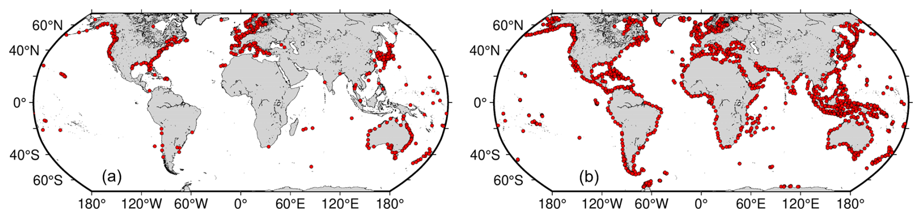
Figure 4 Distribution of (a) 549 tide gauges from PSMSL and (b) 1548 altimeter-based virtual stations from the IAS2024 dataset.

The main steps of the validation procedure are described as follows.

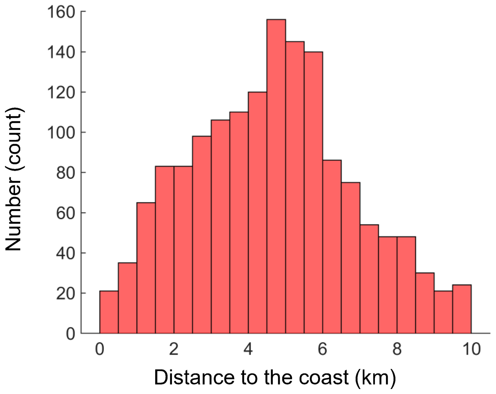
1. The Jason-3 ground tracks which achieve the maximum data points within 100 km from the coast are selected as the nominal ground track. The corresponding 20 Hz offshore distances are directly retrieved from the Jason-3 SGDR product, which are calculated with respect to the Global Self-consistent, Hierarchical, High-resolution Geography Database (GSHHG) dataset (https://www.soest.hawaii.edu/pwessel/gshhg/, last access: 29 September 2024). After that, the single nominal ground track is divided into multiple ground track segments if the distance between consecutive 20 Hz along-track points is larger than 10 km. Only the ground track segments whose nearshore points with distances to the coast being smaller than 10 km and offshore points with distances to the coast being larger than 90 km are used in this study. It is found that there are 1458 ground track segments which fulfill the above criterion, and the distribution of the closest distance to the coast for each ground track segment is shown in Fig. 5.

2. The SCMR-reprocessed 20 Hz along-track SLA estimates from the Jason missions are referenced to the corresponding ground track segments using the nearest-neighbor approach, and a 3σ filter is then applied to the along-track SLA estimates to remove the outliers. The inter-mission SLA biases between different Jason missions are estimated and removed using the overlapping time series method (Peng et al., 2022) before constructing SLA time series with a temporal sampling of 10 d. Then, the 3σ filter is applied to the SLA time series again. In this study, only time series with more than 80 % of available data are used to derive the monthly SLA time series over the period of January 2002 and April 2022.

3. The linear sea level trends are derived from the de-seasoned monthly SLA time series with the Hector software (Bos et al., 2014), which can handle the time series with temporally correlated noise. The stochastic noise models used in this study include the first- and fifth-order autoregressive (i.e., AR1 and AR5), and the autoregressive fractionally integrated moving average (ARFIMA) models. The most appropriate noise model is identified using the lowest mean value of both the Akaike information criterion (AIC; Akaike, 1992) and the Bayesian information criterion (BIC; Schwarz, 1978).

4. The monthly SLA time series of 20 Hz along-track points over the 0–20 km coastal strip are averaged to generate monthly SLA time series at altimeter-based virtual stations. The colocated virtual stations and tide gauges are derived if their distance is smaller than 200 km and the score between them reaches the maximum. The 200 km distance threshold is chosen because of the trade-off between including enough nearby virtual stations and retaining high correlation coefficients. The score is calculated using the correlation coefficient and root mean square (RMS) of the differences between the monthly SLA time series from the virtual station and tide gauge as follows:

   $$\begin{array}{}\text{(7)}& \mathrm{score}={\mathrm{score}}_{\mathrm{cc}}^i\times \mathrm{0.4}+{\mathrm{score}}_{\mathrm{rms}}^i\times \mathrm{0.6},\end{array}$$
   $$\begin{array}{c}{\displaystyle }{\mathrm{score}}_{\mathrm{cc}}^i={\displaystyle \frac{{\mathrm{cc}}_i-min\left(\mathrm{cc}\right)}{max\left(\mathrm{cc}\right)-min\left(\mathrm{cc}\right)}}\times \mathrm{100},\\ {\displaystyle }{\mathrm{score}}_{\mathrm{rms}}^i={\displaystyle \frac{max\left(\mathrm{rms}\right)-{\mathrm{rms}}_i}{max\left(\mathrm{rms}\right)-min\left(\mathrm{rms}\right)}}\times \mathrm{100}.\end{array}$$

The number of colocated stations, the correlation coefficients and the RMS values of the differences between monthly SLA time series from colocated stations, as well as the differences in linear sea level trends derived from the monthly SLA time series are used for the validation.

Figure 5 Distribution of closest distance to the coast for 1548 ground track segments.

The ESA CCI v2.4 20 Hz and the CMEMS L3 1 Hz along-track sea level datasets are also interpolated into the ground track segments using the nearest-neighbor approach. After that, the results from both ESA CCI and CMEMS products are compared with that from the IAS2024 dataset. For comparison, we only use ground track segments that have at least 10 common points with the ESA CCI and 2 common points with the CMEMS within the last 20 km to the coast. When it comes to the correlation coefficients, only those whose p values are smaller than 0.05 are used.

2.3 Application of the IAS2024 coastal sea level dataset

Three applications of coastal altimeter datasets are presented in this study. Firstly, the coastal altimeter datasets can be used to build altimeter-based virtual stations (Benveniste et al., 2020; Cazenave et al., 2022), which is of great importance for monitoring the coastal sea level change and constraining the high-resolution ocean models. To examine the data quality of virtual stations obtained from different coastal strips, the monthly SLA time series of 20 Hz along-track points over 0–10, 5–15 and 10–20 km are averaged for comparison. For clarity, these three types of virtual stations are denoted as onshore, nearshore and offshore virtual stations.

Secondly, the spatial variation in sea level trends can be analyzed because the altimeter provides the along-track sea level trend profile, which help us understand the relative contributions of local and remote processes on coastal sea levels. To address this issue, a linear regression is applied to the along-track sea level trends using the MATLAB function robustfit. The trend differences between nearshore and offshore points in the last 20 km to the coast are then calculated to examine whether there exists significant change (> ±2 mm yr⁻¹) in the along-track sea level trends.

Finally, the VLM estimates can be obtained by calculating the trend estimates from differenced monthly SLA time series between colocated virtual stations and tide gauges, which are used for the comparison with corresponding Global Navigation Satellite System (GNSS) solutions called the University of La Rochelle 7a (ULR7a) (Gravelle et al., 2023). The ULR7a solution is a preliminary version of the reanalysis of 21 years of GPS data from 2000 to 2020 that has been undertaken within the framework of the third data reprocessing campaign of the International GNSS Service (IGS), whose associated vertical velocity field is expressed in the International Terrestrial Reference Frame 2014 (ITRF 2014, Altamimi et al., 2016).

3 Evaluation

3.1 Data availability and precision

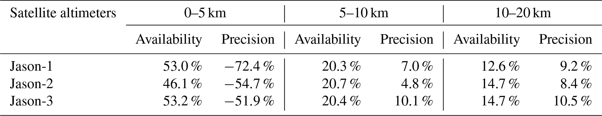
Figure 6 shows the data availability and precision for the official SGDR MLE4 data and SCMR-reprocessed data over different Jason missions. These results are derived after removing the SLA estimates whose absolute values are greater than 1 m. As we can see from the graph, the results from different Jason missions are similar, demonstrating the stability of the Jason missions. Thanks to the open-loop tracking mode (Biancamaria et al., 2018), Jason-3 can recover more reliable SLA estimates than the other two satellites. The results also demonstrate that the SCMR strategy outperforms the official SGDR MLE4 over global coastal oceans. The SCMR can remarkably increase the data availability over the entire 0–20 km distance bands as well as the data precision beyond 6 km to the coast. Note that the higher precision achieved by the official SGDR MLE4 within the 0–6 km distance band can be attributed to the low data availability (Fig. 6a to c) and dedicated data editing strategy applied to the official SGDR product (Peng et al., 2024b). The improved percentage in terms of data availability and precision in different coastal strips (i.e., 0–5, 5–10 and 10–20 km) is summarized in Table 2.

As can be seen from Table 2, the improved percentage for data availability increases with a decreasing offshore distance. In contrast, the data precision shows a declining trend from the offshore in the oceans towards the coast. This result demonstrates that the SCMR strategy can handle multiple waveform types and thus can recover more reliable SLA estimates than the official SGDR MLE4. Within the distance of 0–5 km to the coast, the data precision with respect to the official SGDR MLE4 is not improved, which is mainly attributed to the above reasons. In addition, the range estimates from contaminated waveforms and range/geophysical corrections near the coast are inferior to those over open oceans, which results in a smaller or even negative improvement in the percentage of data precision. Therefore, a dedicated data editing strategy should be developed for the coastal altimeter data as has been done in the SGDR product. Overall, the data availability from SCMR can retain more than 90 % beyond 5 km offshore and more than 70 %–80 % in the last 5 km to the coast (Fig. 6a–c). The data precision can retain centimeter levels (∼ 4.9 cm) over the 10–20 km distance band, increase to 7–9 cm over the 5–10 km distance band and rise up to decimeter levels (∼ 20–23 cm) towards the coast (Fig. 5d–f).

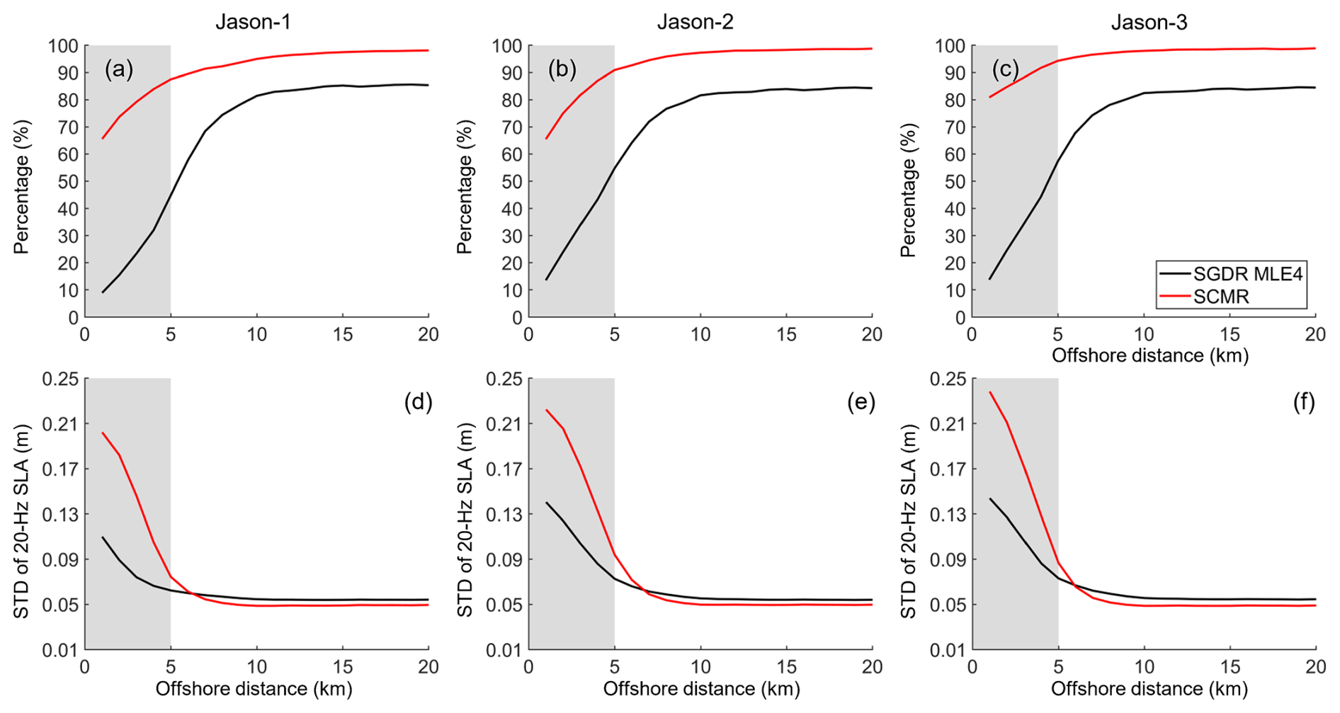
Figure 6 Data availability (a–c) and precision (d–f) for official SGDR MLE4 data (in black) and SCMR-reprocessed data (in red). From left to right, the results for Jason-1, Jason-2 and Jason-3 are shown successively. The data availability is calculated as the percentage of available 20 Hz SLA estimates, while the data precision is represented as the median value of standard deviation (SD) of 20 Hz SLA estimates within 1 s in each 1 km distance band.

Table 2 Improved percentage of the SCMR against the official SGDR MLE4 in terms of data availability and precision over different coastal strips.

The power spectrum and crossover analysis (Fig. 7) further demonstrate the good performance of the SCMR strategy in improving the data availability and reducing noise levels at small spatial scales. Compared to the official SGDR MLE4, the SCMR achieves a reduction in the SLA spectra at scales below 50 km, with the noise level at sub-kilometer scales being 23 % lower than that of the official SGDR MLE4 (Fig. 7a–c). In addition, the crossover analysis shows that the SCMR significantly increases the number of colocated 20 Hz SLA estimates by 44 % while retaining smaller mean differences close to zero and slightly larger standard deviations around 14 cm (Fig. 7d–f).

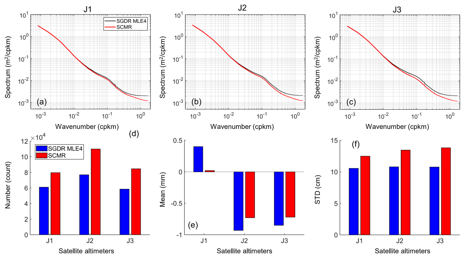
Figure 7 Power spectrum of 20 Hz SLA estimates (a–c) and the number, mean and standard deviation of differences from colocated 20 Hz SLA estimates at crossover points (d–f). J1, J2 and J3 represent Jason-1, Jason-2 and Jason-3 missions, respectively.

3.2 Comparison between IAS2024 and ESA CCI v2.4

In this section, the quality of the IAS2024 coastal dataset is investigated by comparing with the latest ESA CCI v2.4 coastal sea level dataset. The two datasets are compared on 807 ground track segments, which contain at least 10 common points for both IAS2024 and ESA CCI v2.4 datasets over the 0–20 km coastal strip. The selection of 10 common points is meant to guarantee the robustness of the results. To conduct the comparison between these two datasets, we first calculate the point-wise correlation coefficient and RMS of the differences between monthly SLA time series from these two datasets. Then, the averaged correlation coefficients and RMS values for different ground track segments are obtained.

Figure 8 shows the histograms of correlation coefficients and RMS values between detrended and de-seasoned monthly SLA time series from IAS2024 and ESA CCI v2.4 datasets for different ground track segments over global coastal oceans. As we can see from the graph, the consistency of the monthly SLA time series between these two datasets is good at the global scale, which is consistent with our previous study in the Australian coastal zone (Peng et al., 2022). Relatively high correlation coefficients (>0.4) are achieved in most cases. As a result, the mean correlation coefficient between IAS2024 and ESA CCI v2.4 datasets is 0.59, while the corresponding RMS values mostly varying between the range of 40 and 80 mm. The spatial distribution of both correlation coefficients and RMS values (Fig. 9) reveals that the discrepancy between IAS2024 and ESA CCI v2.4 datasets is only observed on the west coast of South America.

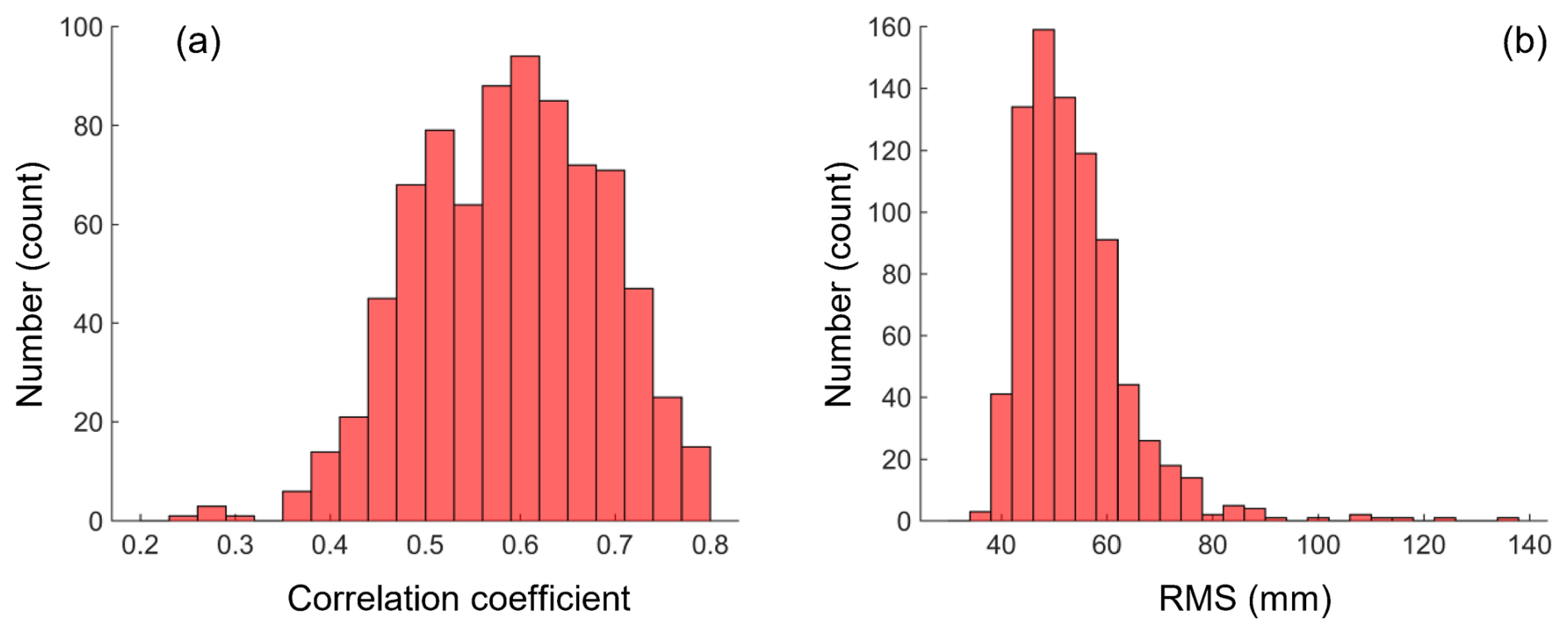
Figure 8 Distribution of averaged correlation coefficients (a) and RMS values (b) between detrended and de-seasoned monthly SLA time series from IAS2024 and ESA CCI v2.4 datasets for different ground track segments over the 0–20 km coastal strip.

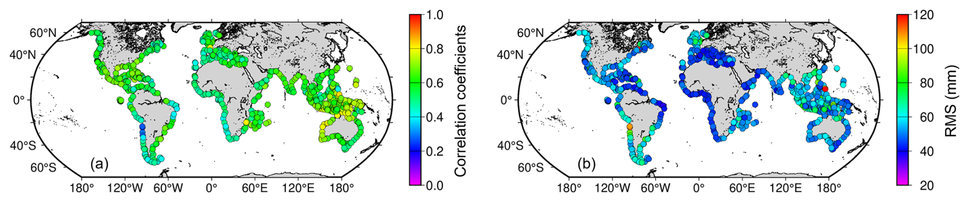
Figure 9 Spatial distribution of averaged correlation coefficients (a) and RMS values (b) between detrended and de-seasoned monthly SLA time series from IAS2024 and ESA CCI v2.4 datasets for different ground track segments over the 0–20 km coastal strip.

In addition to the comparison of monthly SLA time series, we also analyze the sea level trends from these two datasets over a similar period. First, the point-wise sea level trends and trend uncertainties are derived from both IAS2024 and ESA CCI v2.4 datasets. Then, the trend differences and uncertainties at common points are averaged for each ground track segment. Finally, the histograms of averaged trend differences and trend uncertainties are shown in Fig. 10.

As we can see from the graph, the trend differences between them are predominantly within the range between −4 and 6 mm yr⁻¹, with the mean of trend differences being 1.32 ± 2.40 mm yr⁻¹ (Fig. 10a). The trend uncertainties for both datasets are similar, varying between 0.5 and 2.0 mm yr⁻¹ (Fig. 10b). This result implicates that the sea level trends derived from the IAS2024 dataset are generally higher than those from the ESA CCI v2.4 dataset, which is in line with our previous findings (Peng et al., 2022, 2024a). The reason behind this may be attributed to the different data processing techniques adopted, especially the methods used to estimate the inter-mission SLA biases (Peng et al., 2022).

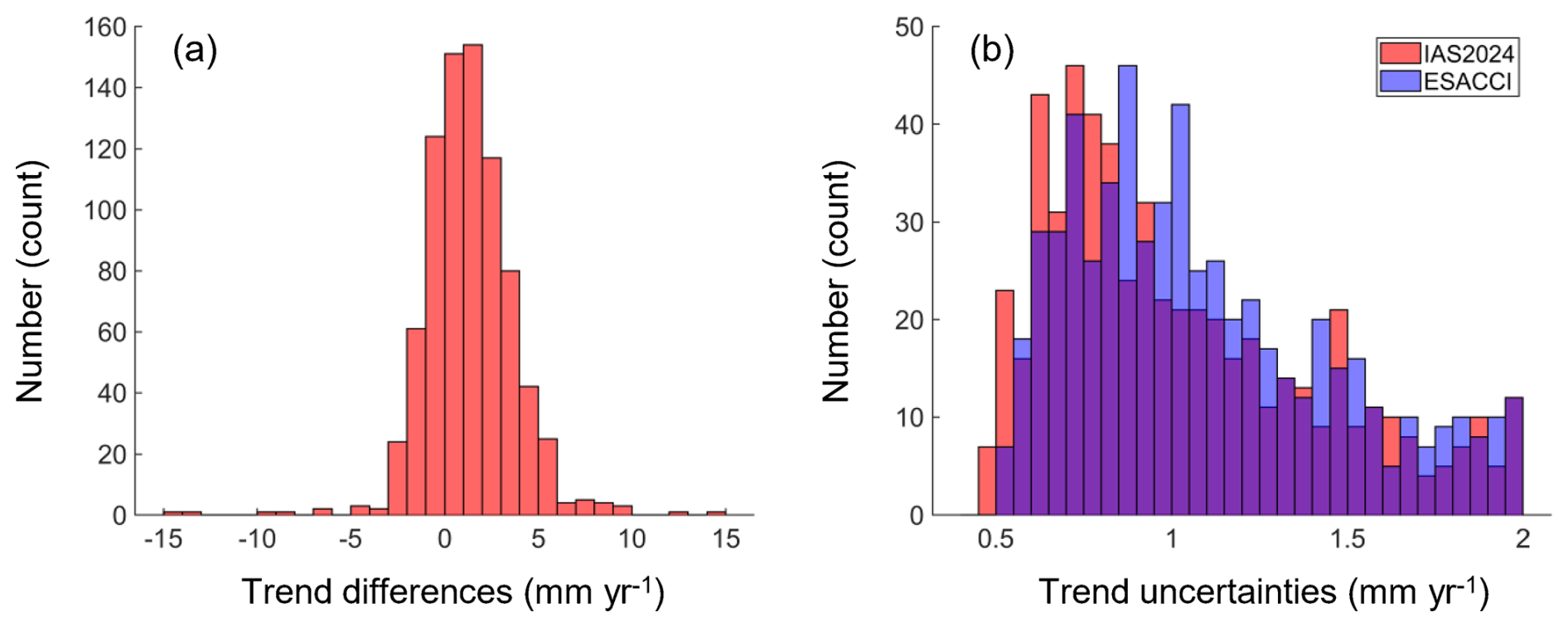
Figure 10 Distribution of (a) averaged trend differences from de-seasoned monthly SLA time series between IAS2024 and ESA CCI v2.4 datasets as well as (b) trend uncertainties for different ground track segments over the 0–20 km coastal strip. The violet bars in (b) are the overlaps between IAS2024 and ESA CCI.

At last, the tide gauge records from the PSMSL are deemed as the ground truth and used for the validation of these two datasets. Table 3 summarizes the number of colocated virtual stations and tide gauges for both IAS2024 and ESA CCI v2.4 datasets. In addition, the mean of correlation coefficients and RMS values and the mean of trend differences between altimeter and tide gauge are listed in Table 3. As illustrated by the table, the number of colocated stations for the IAS2024 dataset (290) is similar to that for the ESA CCI v2.4 dataset (293). This is because the same ground track segments are used for comparison. The comparable performance is also observed for these two datasets in terms of correlation coefficients and RMS values. However, these two datasets differ in the trend differences between the altimeter and tide gauge at the global scale. As reported by previous studies (e.g., Watson et al., 2015; Wöppelmann and Marcos, 2016), the VLMs are canceled out on average along the world's coastlines. Therefore, it is reasonable to assume that the averaged trend difference between the altimeter and tide gauge is close to zero at the global scale. The result from the IAS2024 dataset is thus consistent with this assumption, even though it is not a true global scale, as the mean of trend differences is −0.26 ± 3.57 mm yr⁻¹, which demonstrates the good performance of the IAS2024 dataset in monitoring the coastal sea levels. However, a negative trend difference (−1.50 ± 3.31 mm yr⁻¹) is shown in Table 3 when validating the ESA CCI v2.4 dataset against tide gauge records. This may be ascribed to the fact that there exists a systematic bias (1.32 ± 2.40 mm yr⁻¹) between sea level trends from IAS2024 and ESA CCI v2.4 datasets.

Table 3 Validation results of IAS2024 and ESA CCI v2.4 datasets against tide gauge records from PSMSL. Note that the correlation coefficients and RMS values are derived from the detrended and de-seasoned monthly SLA time series, while the sea level trends are derived from the de-seasoned monthly SLA time series.

Overall, the above comparison results reveal the good consistency between IAS2024 and ESA CCI v2.4 datasets over the same ground track segments, though there exists a systematic bias between their sea level trends. It is also noted that the IAS2024 dataset can achieve higher spatial coverage because the ESA CCI v2.4 dataset has no data in places such as Japan and northern Europe (see Sect. 4.1 and 4.2).

3.3 Comparison between IAS2024 and CMEMS L3 along-track products

The IAS2024 coastal dataset is also compared with the CMEMS L3 1 Hz along-track product. Note that 830 ground track segments which contain at least two common points for these two datasets over the 0–20 km coastal strip are used for comparison. The selection of two common points is made because the CMEMS L3 product provides the 1 Hz (∼ 7 km along-track) instead of 20 Hz (∼ 300 m along-track) SLA data.

Figure 11 shows the histograms of averaged correlation coefficients and RMS values between detrended and de-seasoned monthly SLA time series from the IAS2024 and CMEMS datasets for different ground track segments. As we can see from the graph, correlation coefficients mostly vary between 0.4 and 0.8, and the RMS values are mainly smaller than 60 mm. This result is in line with the comparison result between IAS2024 and ESA CCI v2.4 datasets shown in Sect. 3.2, indicating good consistency between IAS2024 and CMEMS at the global scale. The spatial distribution of both correlation coefficients and RMS values (Fig. 12) further reveals that the low correlation coefficients between IAS2024 and CMEMS datasets are again observed in the west coast of South America.

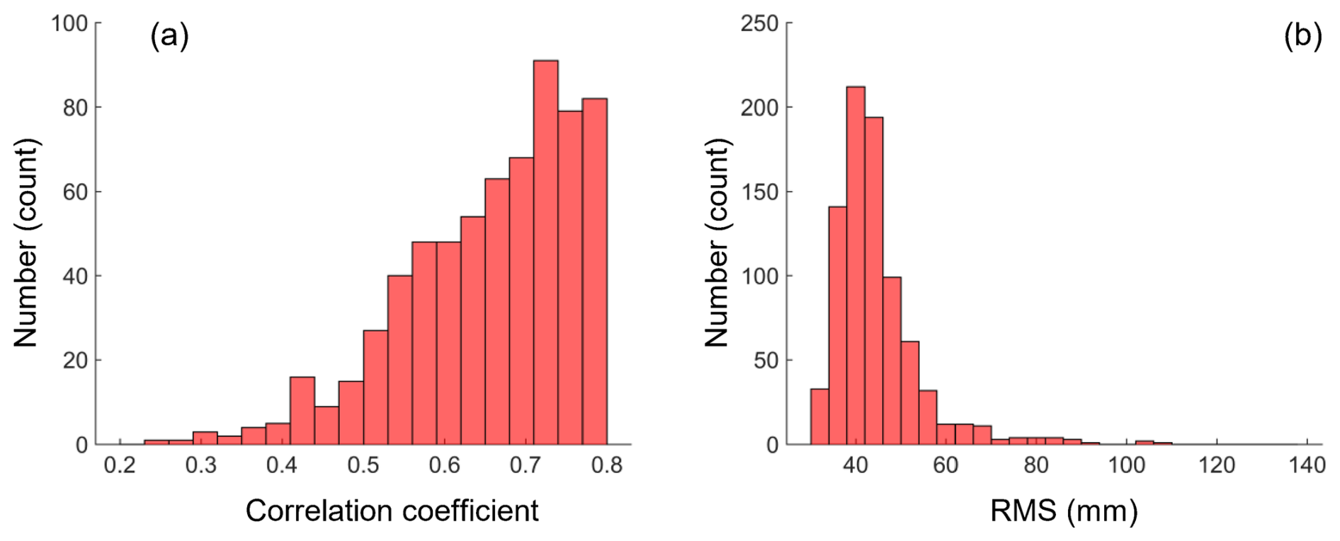
Figure 11 Same as Fig. 7 but for the comparison between IAS2024 and CMEMS L3 along-track datasets.

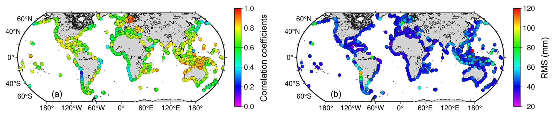
Figure 12 Same as Fig. 8 but for the comparison between IAS2024 and CMEMS L3 along-track datasets.

Figure 13 shows the histograms of averaged trend differences and uncertainties. As illustrated by the graph, most of the trend differences vary between ±4 mm yr⁻¹, while the trend uncertainties are within the range between 0.5 and 2 mm yr⁻¹. The mean trend difference between IAS2024 and CMEMS is −0.18 ± 2.17 mm yr⁻¹, indicating the systematic bias between these two datasets is relatively small. This result is in contrast with that between IAS2024 and ESA CCI v2.4 (see Sect. 3.2). The reason behind this requires further investigation, which will be the theme of our future work.

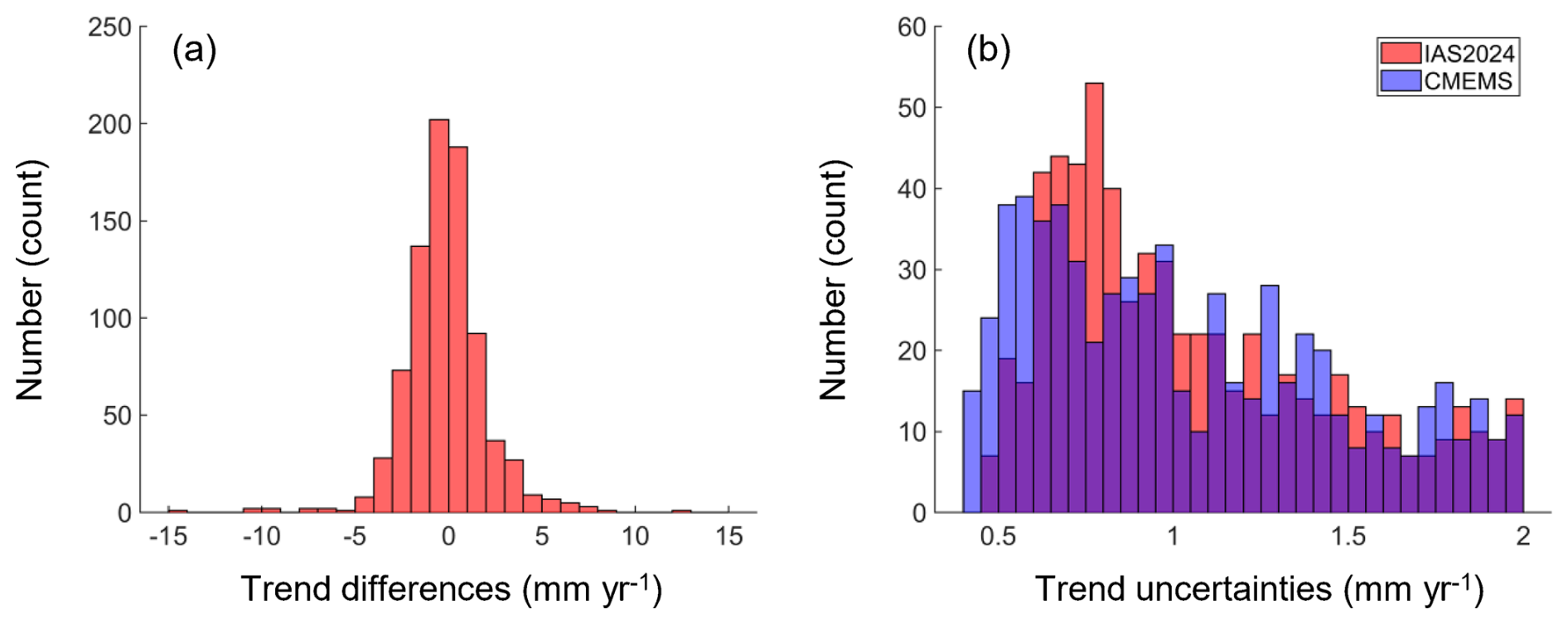
Figure 13 Same as Fig. 9 but for the comparison between IAS2024 and CMEMS L3 along-track datasets. The violet bars in (b) are the overlaps between IAS2024 and CMEMS.

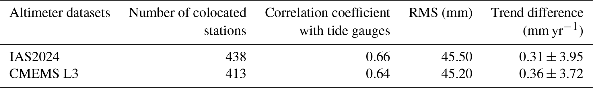
In the end, the validation results against tide gauge records for IAS2024 and CMEMS are summarized in Table 4. As we can see from the table, the results for these two datasets are in good agreement. Moreover, the trend differences derived from these two datasets are similar and close to zero, which is in contrast with the result from the ESA CCI v2.4 dataset (−1.50 ± 3.31 mm yr⁻¹). The reason behind this may be attributed to the fact that the systematic bias (−0.18 ± 2.17 mm yr⁻¹) of sea level trends between IAS2024 and CMEMS datasets is relatively small (Fig. 13a), while that for the ESA CCI v2.4 dataset is larger (1.32 ± 2.40 mm yr⁻¹; Fig. 10a).

Table 4 Same as Table 3 but for the comparison between IAS2024 and CMEMS L3 along-track datasets.

4 Applications of coastal altimeter datasets

The coastal altimeter datasets are an important complement to the existing tide gauge networks considering their higher spatial coverage (Fig. 4). As we can see from the graph, the altimeter-based virtual stations are distributed along the world's coastlines, while the tide gauges, which have continuous data records over the period from 2002 to 2022, are mostly situated in Japan, Australia, North America and Western Europe. Moreover, the altimeter measures the absolute sea levels relative to the ITRF, which are not affected by the VLM and thus help us investigate the spatial variation of sea level changes from the offshore in the oceans to the coast.

In the following sections, we focus on three applications of coastal altimeter datasets. The first is to build altimeter-based virtual stations along the world's coastlines, which can be used to monitor the coastal sea level changes where tide gauges are unavailable. The second is to investigate whether there exist significant trend differences between offshore and nearshore oceans in the last 20 km to the coast. The former is of paramount importance for coastal management and risk adaptation (Fox-Kemper et al., 2021), while the latter gives us insights into the role of small-scale processes in changing the coastal sea level trends (Woodworth et al., 2019; Harvey et al., 2021; Cazenave et al., 2022). The last is to calculate the VLM estimates by combining virtual stations and tide gauges, which provides a way to validate the VLM estimates from GNSS stations (Wöppelmann and Marcos, 2016).

4.1 Altimeter-based virtual stations

To better monitor the coastal sea levels, it is expected that the virtual stations are located as close to the coast as possible. However, the precision of altimeter data degrades with a decreasing offshore distance to the coast (Fig. 6). Therefore, it is necessary to investigate which coastal strip is preferable for building the virtual stations. Here, we generate three different sets of virtual stations following the methods described in Sect. 2.2 using the IAS2024 dataset, and refer them as the onshore, nearshore and offshore virtual stations according to their distances to the coast. Note that the onshore, nearshore and offshore stations are generated from the altimeter data within 0–10, 5–15 and 10–20 km distance bands, respectively.

Figure 14 shows the comparison results between onshore virtual stations and tide gauges in terms of correlation coefficients and RMS values. As can be seen from the graph, the high correlation coefficients (> 0.6) and low RMS values (<60 mm) are observed along the world's coastlines, which indicates a good quality of the onshore virtual stations. Better results can be achieved by the nearshore and offshore virtual stations in terms of a higher number of virtual stations, while the high correlation coefficients and low RMS values are retained (Table 5). This suggests that the coastal sea level signals are highly correlated over the spatial scales of ∼ 20 km. Therefore, the correlation coefficient between nearshore and offshore time series can be an important indicator in evaluating data quality.

It is also noted that low correlation coefficients and high RMS values are observed at some onshore stations such as the east coast of North America and the west coast of South America (Fig. 14), which can be attributed to three causes. Firstly, the VLM affects the comparison between the tide gauge and altimeter at the local scale (Wöppelmann and Marcos, 2016). Secondly, the colocated stations are usually tens to hundreds of kilometers away, from which they measure different sea level signals (Vinogradov and Ponte, 2010). Finally, the coastal environments (e.g., bathymetry, sea states and morphology) can be quite different from the nearby offshore regions, which leads to the significant deterioration of range estimates and range/geophysical corrections (e.g., geocentric ocean and loading tide corrections, wet tropospheric correction, sea state bias correction, and dynamic atmospheric correction) (Gommenginger et al., 2011; Abele et al., 2023; Peng et al., 2024b).

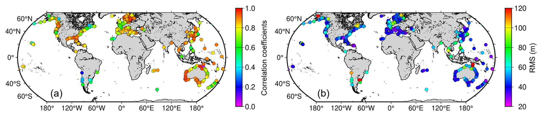
Figure 14 Comparison results in terms of (a) correlation coefficient and (b) root mean square (RMS) of the differences between monthly time series from onshore virtual stations and tide gauges. The onshore virtual stations are generated using the 20 Hz along-track altimeter data within the 0–10 km coastal strip.

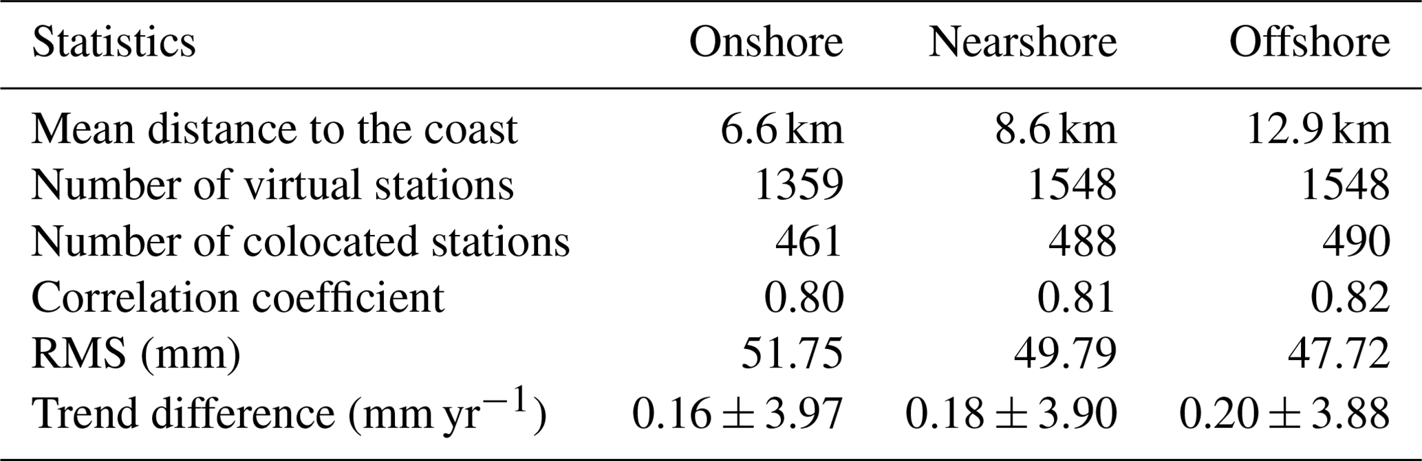
Compared to the nearshore and offshore stations, the onshore stations are more likely to be affected by land contamination because they include the altimeter data within 5 km of the coast, leading to the smaller number of virtual stations (1359 vs. 1548). However, the observation degradation does not seem to be remarkable, and the closure of the trend difference between satellite and tide gauge at the global scale is unchanged. This result implies that the altimeter data within 0–5 km of the coastal strip can be used when the dedicated editing strategy is applied. In addition, the sea level trends obtained from the altimeter data closer to the coastline are more consistent with those from tide gauge records at the global scale. Therefore, we suggest that the 5–15 km coastal strip is the most suitable for building the virtual stations considering the trade-off between the closest distances to the coast and the reliability of the data quality.

Table 5 Comparison results between altimeter-based virtual stations and tide gauges. The correlation coefficients and RMS values are derived from the monthly SLA time series between virtual stations and tide gauges, while the trend estimates are obtained from the de-seasoned SLA time series.

4.2 Spatial variations of sea level trends towards the coast

As reported by previous studies (Deng et al., 2011; Benveniste et al., 2020; Harvey et al., 2021), the coastal sea level trends measured by tide gauges differ from altimeter-derived sea level trends offshore. However, it is uncertain whether the trend discrepancy is due to the different ocean dynamic processes measured by the tide gauge and altimeter or the VLM (Cazenave et al., 2022). Therefore, a good way to solve this issue is to explore the spatial variation of altimeter-derived sea level trends from the offshore to the nearshore in the last 20 km to the coast. For example, Cazenave et al. (2022) compared the coastal trends (within 4–5 km) with the offshore trends (within 15–17 km) and found no significant differences (within ±2.0 mm yr⁻¹) at 78 % of the 756 virtual stations. Note that the degradation of altimeter data within 5 km of the coast affects the results from the above method. To avoid this problem, a robust linear regression is applied to the along-track trends using the MATLAB function robustfit in this study. This regression function is chosen because it can alleviate the impact of outliers on the estimation procedure from our experimental tests. The trend differences between nearshore and offshore are then calculated. If the absolute trend differences are smaller than 2.0 mm yr⁻¹, it is considered that there is no significant discrepancy between nearshore and offshore sea level trends. Otherwise, the increasing (decreasing) trend is detected if the trend difference is larger than 2.0 mm yr⁻¹ (smaller than −2.0 mm yr⁻¹).

Figure 15 presents four examples of 20 Hz along-track sea level trends against distance to the coast for both IAS2024 and ESA CCI v2.4 datasets. As we can see from the graph, the spatial variations of 20 Hz along-track trends show different patterns (i.e., constant, increasing or decreasing) depending on different geolocations. In addition, the smooth variations of 20 Hz along-track trends at the spatial scales of ∼ 300 m is observed (Fig. 15a to c). Therefore, the abrupt fluctuation of 20 Hz along-track trends near the coast (Fig. 15d) can be attributed to the degradation of altimeter data.

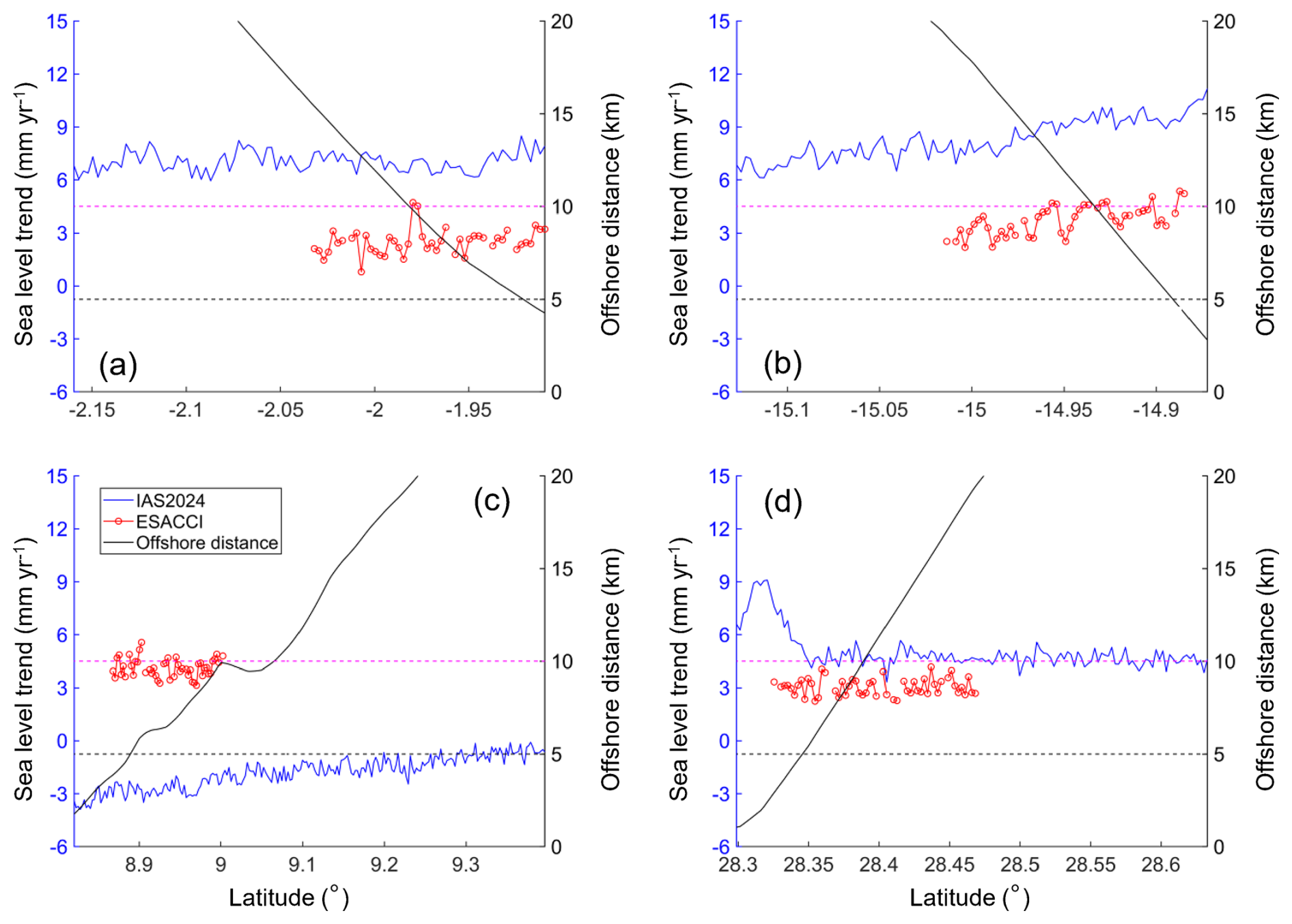
Figure 15 Examples of 20 Hz along-track sea level trends against distance to the coast for both IAS2024 and ESA CCI v2.4 datasets. Panels (a) to (d) show constant, increasing and decreasing trends as well as an abrupt fluctuation towards the coast. Horizontal dashed lines indicate distances to the coast at 5 km (in black) and 10 km (in magenta).

The statistical results of trend differences over global coastal oceans for these two datasets are illustrated in Fig. 16. As demonstrated by the graph, there is no significant difference (within ±2 mm yr⁻¹, i.e., of the maximum level of trend uncertainties) at 97 % of the 1548 ground track segments. In the remaining 3 %, we observe either an increasing trend (1.5 %) or a decreasing trend (1.5 %). This result is consistent with that from the ESA CCI v2.4 dataset, where 90 % of the 807 ground track segments show no trend difference, and the percentage of the decreasing trend (5 %) is equal to that of the increasing trend (5 %). It is also observed that there is no any concentration of coastal trends departing from offshore trends in a particular region (Fig. 17), which means that the increasing or decreasing trends can occur along the world's coastlines.

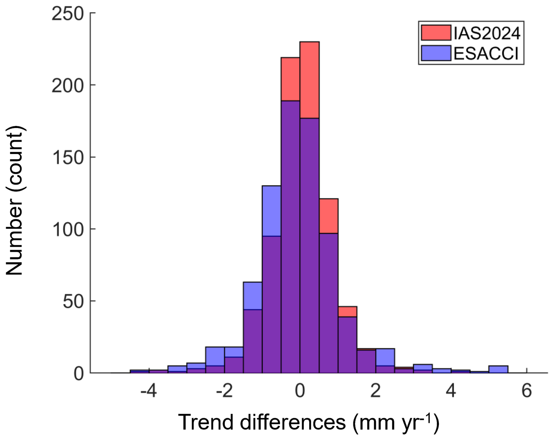
Figure 16 Trend differences between nearshore and offshore stations for the IAS2024 and ESA CCI v2.4 datasets.

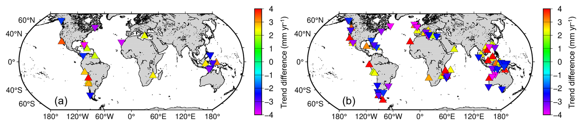
Figure 17 Trend differences between nearshore and offshore stations in the last 20 km from the coast for the IAS2024 (a) and ESA CCI v2.4 (b) datasets. Triangles and inverse triangles correspond to increasing and decreasing trends, respectively.

The trend differences in most places are insignificant, which may be ascribed to two aspects. Firstly, most of the trend uncertainties are relatively large (∼ 0.5–2.0 mm yr⁻¹), which makes them insensitive to the small changes in sea level trends. Secondly, the small-scale process-induced variations (e.g., by coastal currents, winds, waves and freshwater input in river estuaries) do not significantly affect the coastal sea level trends because the sea level variation over longer timescales is more likely to be affected by the remote signals from open oceans (Han et al., 2019). It is also noted that the trend differences are remarkable in some places, which motivates us to investigate the reasons behind the trend variation. For instance, a recent study by Piecuch et al. (2018a) has demonstrated the role of river discharge in affecting the coastal sea levels over interannual or longer timescales. Moreover, the high-resolution ocean models (with a grid mesh smaller than 1 km) contribute to the systematic quantification of coastal phenomena causing the reported trend to increase or decrease near the coast (Marti et al., 2021; Gouzenes et al., 2020; Dieng et al., 2021). However, the high-resolution ocean models are currently not available over global coastal oceans (Han et al., 2019; Melet et al., 2020; Laignel et al., 2023). Therefore, more efforts should be made in the future to improve our understanding of present-day coastal sea level changes and to improve the ability of climate models to simulate future sea levels in highly populated and vulnerable coastal regions of the world.

4.3 Vertical land motion

The combination of satellite radar altimetry and tide gauge data can be used to estimate the VLM (e.g., Wöppelmann and Marcos, 2016). Figure 18 shows the sea level trends at virtual stations and tide gauges, respectively. As we can see from the graph, the remarkable differences between the altimeter and tide gauge are concentrated in the coasts of the east US and northern Europe. This is because northern Europe suffers from large uplift rates due to glacial isostatic adjustment (GIA), while the US east coast is exposed to large coastal subsidence rates due to the subsurface fluid withdrawal and the response to GIA (Wöppelmann and Marcos, 2016; Piecuch et al., 2018b; Harvey et al., 2021).

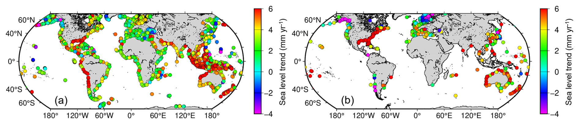
Figure 18 Sea level trends over the period of January 2002 and April 2022 at altimeter-based virtual stations and tide gauges along the world's coastlines. Panel (a) shows the results of onshore (0–10 km) virtual stations from the IAS2024 dataset, while (b) presents the results from the PSMSL tide gauges.

The VLM (Fig. 19) is derived in this study from the difference between the de-seasoned monthly SLA time series of the altimeter and tide gauge (i.e., ALT − TG) that follows the method described in Sect. 2.3. As can be seen, the large uplift rates (>2 mm yr⁻¹) are observed in northern Europe and the northwest coast of Canada, suggesting that the GIA-related radial crust displacement is significant in these regions. In addition, the upper lift rates are also observed along the southwest coast of South America. The large subsidence rates ($<-\mathrm{2}$ mm yr⁻¹), however, are presented along the coast of the northern Gulf of Mexico, where the groundwater extraction is significant (Wöppelmann and Marcos, 2016; Harvey et al., 2021). Along the Australian coastline, both the uplift and the subsidence rates are observed but dominated by subsidence rates along the northeast coast. When it comes to the western Europe and Japan, the VLM estimates show large variations dependent on different locations, with the overall median values being close to zero for different sets of virtual stations.

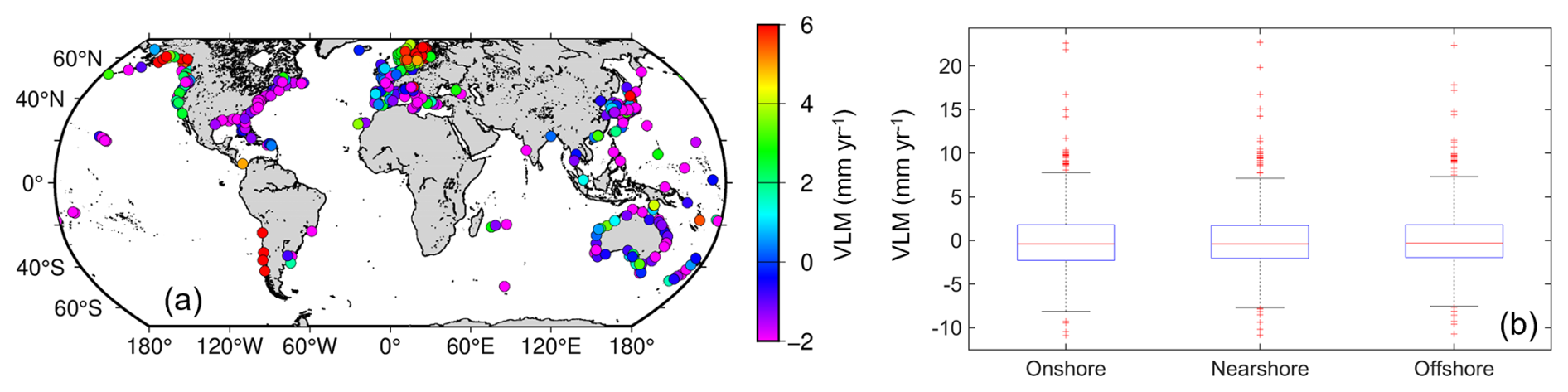
Figure 19 VLM estimates derived from the combination of virtual stations and tide gauges. Panel (a) shows the results of onshore virtual stations, while (b) shows the boxplot of the VLM estimates from onshore, nearshore and offshore virtual stations. On each box, the central mark indicates the median, and the bottom and top edges of the box indicate the 25th and 75th percentiles, respectively. The whiskers present the most extreme data points outside the percentiles, while the outliers are plotted individually using the + symbol.

Figure 19b illustrates that the VLM estimates from onshore virtual stations are in accordance with those from nearshore and offshore stations, with median values being close to zero. This result further demonstrates that nearshore and offshore trends in the last 20 km to the coast are identical in most cases, which is consistent with the results shown in Sect. 4.1. To assess the robustness of the results, the VLM estimates from GNSS observations are used for comparison. The PSMSL tide gauges and the nearest ULR7a GNSS stations are colocated if their distances are within 10 km. As a result, the number of colocated stations is 166, and the comparison results are shown in Fig. 20.

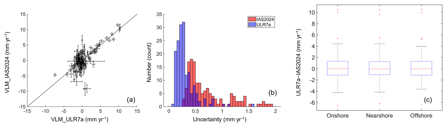
Figure 20 Comparison between ULR7a-derived VLM estimates from GNSS observations and IAS2024-based virtual stations. Panels (a) to (c) show the scatterplot between IAS2024 onshore virtual stations and GNSS stations; the uncertainties in VLM from IAS2024 and GNSS; and the boxplot of the difference in VLM for onshore, nearshore and offshore stations, respectively. In (a), the horizontal and vertical error bars represent the uncertainties in GNSS-derived and altimeter-derived VLM, respectively.

As can be seen, the VLM uncertainties from ULR7a are mostly within the range between 0 and 0.5 mm yr⁻¹, while the corresponding uncertainties from the combination of the tide gauge and altimeter vary between 0.5 and 2 mm yr⁻¹ (Fig. 20a and b). The uncertainties from the combination of tide gauge and altimeter are slightly larger, which can be attributed to the different spatial and temporal sampling manners between altimeter and tide gauge datasets, the different geographical locations between altimeter-based virtual stations and tide gauges, and the short time span of the time series. Figure 20c shows that the VLM estimates from the combination of the altimeter and tide gauge agree well with those from GNSS observations in most cases, with the differences being smaller than ±1.5 mm yr⁻¹. The mean of the differences is 0.12 mm yr⁻¹, with an SD of 2.27 mm yr⁻¹ for onshore virtual stations, while similar values are 0.14 (0.16) mm yr⁻¹ and 2.16 (2.16) mm yr⁻¹ for nearshore (offshore) virtual stations. Therefore, the results from altimeter-based virtual stations can be used as an independent source to validate the VLM estimates from GNSS observations.

5 Data availability

The IAS2024 coastal sea level dataset is available as open access at https://doi.org/10.5281/zenodo.13208305 as network Common Data Form (netCDF) files (Peng et al., 2024c). This dataset includes monthly SLA time series at 20 Hz along-track points for different ground track segments and at onshore, nearshore and offshore virtual stations. Moreover, it contains the corresponding SLA time series at 10 d cycle timescales. The FES2014 geocentric ocean and loading tide corrections, the MOG2D dynamic atmospheric correction, and the CLS22 MSS over the same timescales are also provided for studying oceanography and geodesy.

6 Conclusions

A new reprocessed 20 Hz coastal sea level dataset, namely, IAS2024, for monitoring sea level changes along the world's coastlines has been presented, along with the first evaluations. The Seamless Combination of Multiple Retrackers (SCMR) processing strategy is adopted to generate the coastal 20 Hz SLA estimates from Jason missions over the period from January 2002 and April 2022. The main conclusions of this study are summarized as follows.

The SCMR strategy has significantly increased the data availability when compared to the official SGDR MLE4 retracker, with the improvement percentage varying between 12.6 % and 53.2 % depending on the coastal strip. A moderate improvement (4.8 %–10.1 %) of data precision brought by the SCMR strategy is also observed, mainly because the SCMR can reduce the variability of the SLA spectrum below the wavelength of 50 km. As a result, the data availability of SCMR-reprocessed Jason data can retain more than 90 % of information beyond 5 km offshore and more than 70 %–80 % onshore within 5 km to the coast. In addition, the precision of 20 Hz SLA estimates can be retained at centimeter levels (5–9 cm) over the 5–20 km distance band and at decimeter levels (∼ 20–23 cm) towards the coastline. These results suggest that the IAS2024 dataset generated with the SCMR strategy has the potential to provide reliable SLA estimates for monitoring coastal sea level changes.

The performance of the IAS2024 dataset has been evaluated and validated through comparisons of the monthly SLA time series, as well as the sea level trends, with those from the PSMSL tide gauge records and independent altimeter datasets (i.e., ESA CCI v2.4 20 Hz and CMEMS L3 1 Hz along-track sea level datasets). The good consistency between different altimeter datasets is observed over global coastal oceans in terms of high correlation coefficients (>0.4) and low RMS values (40–60 mm). The sea level trends from the IAS2024 dataset are on average 1.32 ± 2.40 mm yr⁻¹ higher than those from the ESA CCI v2.4 dataset and are similar to those from the CMEMS L3 product (−0.18 ± 2.17 mm yr⁻¹). These may be attributed to the different data processing techniques adopted, especially the methods used to estimate the inter-mission biases. The validation against tide gauges demonstrates that the IAS2024 and CMEMS datasets achieve the closure of trend differences (0.16 ± 3.97 and 0.36 ± 3.72 mm yr⁻¹) at the global scale, which are very close to the theoretical value of zero, demonstrating the good performance of the IAS2024 dataset in monitoring the coastal sea levels. In contrast, a negative bias (−1.50 ± 3.31 mm yr⁻¹) is found for the ESA CCI v2.4 dataset.

Three applications of the IAS2024 dataset are conducted in this study, which give us insights into how dedicated coastal sea level datasets can be used for ocean communities and policymakers. Firstly, altimeter-based virtual stations are built along the world's coastline over 0–10 km (1359), 5–15 km (1548) and 10–20 km (1548) coastal strips, which are denoted as onshore, nearshore and offshore virtual stations, respectively. The results show that virtual stations achieve a much higher spatial coverage than the PSMSL tide gauges (1548 vs. 549), which contribute to the analysis of coastal sea level changes in places where tide gauge data are unavailable. It is also found that the onshore stations are affected by the degradation of altimeter data within 5 km of the coast, leading to a decrease in the number of virtual stations from 1548 to 1359.

Secondly, the spatial variations of the linear sea level trends are evaluated with both IAS2024 and ESA CCI v2.4 datasets. The results from these two datasets show a similar pattern but with different magnitudes at the global scale, with the constant trend being dominant (97 % for IAS2024 and 90 % for ESA CCI v2.4). This result indicates that the local processes have little impact on coastal sea level changes over longer timescales, which is consistent with the findings revealed by Cazenave et al. (2022). Besides, the reasons leading to the increasing or decreasing trends found in some places should be further investigated with the use of high-resolution ocean models, which will be the theme of our future work. Finally, the VLM estimates derived from the combination of the altimeter and tide gauge are consistent with those from the GNSS stations, with the mean of differences in VLMs being 0.12 ± 2.27 mm yr⁻¹ for onshore stations. Therefore, the altimeter-derived VLM estimates can be used as an independent data source for validating GNSS solutions.