Exploring multi-decadal time series of temperature extremes in Australian coastal waters

The intensity and frequency of extreme ocean temperature events, such as marine heatwaves (MHWs) and marine cold spells (MCSs), are expected to change as our oceans warm. Little is known about marine extremes in Australian coastal waters, particularly below the surface. Here we introduce a multi-decadal observational record of extreme ocean temperature events starting in the 1940s and 1950s between the surface and the bottom (50–100 m) at four long-term coastal sites around Australia: the Australian Multi-Decadal Ocean Time Series EXTreme (AMDOT-EXT) data products (https://doi.org/10.26198/wbc7-8h24, Hemming et al., 2024). The data products include indices indicating the timing of extreme warm and cold temperature events, their intensity and the corresponding temperature time series and climatology thresholds. We include MHWs, MCSs and shorter-duration heat spikes and cold spikes. For MHWs and MCSs, which are defined as anomalies above the daily varying 90th and 10th percentiles, respectively, and lasting more than 5 d, we also provide further event information, such as their category and onset and decline rates. The four data products are provided as CF-compliant NetCDF files, and it is our intention that they be updated periodically. It is advised that data users seek the latest data product version. Using these multi-decadal data products, we show the most intense and longest extreme temperature events at these sites, which have occurred below the surface. These data records highlight the value of long-term full water column ocean data for the identification of extreme temperature events below the surface.

1 Introduction

Long-term ocean temperature records have become extremely valuable as the oceans warm due to anthropogenic climate change (Masson-Delmotte et al., 2021). This warming is expected to affect the characteristics of extreme temperature events such as marine heatwaves (MHWs) and marine cold spells (MCSs) (Oliver et al., 2018; Frölicher et al., 2018; Schlegel et al., 2021) (which are often defined as lasting 5 d or more), and their shorter variants lasting less than 5 d are referred to as heat spikes (HSs) and cold spikes (CSs) (Hobday et al., 2016; Schlegel et al., 2021). Extreme warm and cold water events are having an impact on marine ecosystems, including coral bleaching (Zapata et al., 2011; Hughes et al., 2017), mass mortality of organisms (Woodhead, 1964; Garrabou et al., 2009; Santos et al., 2016) and shifts in the distribution of marine species (Vergés et al., 2014; Firth et al., 2015; Wernberg et al., 2016; Smale et al., 2019). The health of a marine ecosystem influences the amount of life that it can sustain, and thus MHWs and MCSs can affect fisheries and the blue economy (Smith et al., 2021). Globally, MHWs are expected to become more intense, more frequent and longer-lasting as a result of climate change (Oliver et al., 2018; Frölicher et al., 2018), while the opposite is expected for MCSs (Schlegel et al., 2021). Similarly, in waters off south-eastern Australia, there has been an upward trend in surface MHW frequency, intensity and duration between 1982 and 2020 (Kajtar et al., 2021).

There are numerous examples of extremely warm or cold temperatures being recorded in Australian coastal waters. In 2011 off Western Australia, low sea level pressure linked to a strong La Niña intensified the Leeuwin Current, leading to MHW conditions at the surface. This MHW lasted for weeks and maximum intensities peaked at 5 ^∘C warmer than the 2000–2009 average climatology (Feng et al., 2013). In 2015/2016 off eastern Tasmania, the East Australian Current (EAC) extension waters were warmer than average, leading to MHW conditions. The MHW at the surface persisted for 251 days between September 2015 and May 2016 and regionally averaged sea surface temperature anomalies were between 1.5 and 3 ^∘C warmer than average between November 2015 and February 2016 (Oliver et al., 2017). A similar event also occurred in this region during austral summer 2017/2018 (Kajtar et al., 2022). MHW conditions persisted for approximately 3 months, with mean Tasman Sea surface temperatures 1 to 3 ^∘C above the 1983–2012 seasonal climatology (Kajtar et al., 2022). Finally, in austral summer 2021/2022 the position of the EAC jet and its eddies off south-eastern Australia had a crucial role in driving MHW and MCS conditions in coastal waters close to Sydney. A MHW occurred in December 2021 and February 2022, while a MCS occurred in January 2022 (Li et al., 2023).

Due to data availability in space and time, many MHW and MCS studies are focused on the surface (e.g. Oliver et al., 2018; Frölicher et al., 2018; Schlegel et al., 2021; Kajtar et al., 2021; Marin et al., 2021). Schaeffer and Roughan (2017) were amongst the first to analyse MHWs at multiple depths between the surface and the bottom at a 65 and 100 m coastal site off Sydney, Australia. Using in situ data from these sites, they showed that MHWs are often at a maximum intensity below the surface, illustrating the importance of understanding the complex structure of MHWs below the surface.

Some of the longest sub-surface temperature measurements in the Southern Hemisphere are located at four Australian coastal sites (Roughan et al., 2022a). One site is located on the western coast, influenced by the Leeuwin Current system, and three sites are located on the eastern coast influenced by the EAC system (Roughan et al., 2022a). These temperature records began as early as the 1940s and continue to the present day. The long temperature records at these sites are valuable for investigating ocean temperature variability on many timescales (Hemming et al., 2020; Roughan et al., 2022a, b) over periods of more than 65 years. Additionally, they are valuable for the investigation of marine extremes, such as the characteristics of HSs and CSs as well as MHWs and MCSs in more recent decades, when high-frequency observations became available (Schaeffer and Roughan, 2017).

Here we describe four unique data products, one for each of Australia's long-term national reference stations described in Sect. 2, which can be used for analysing individual or multiple extreme temperature events, such as HSs, CSs, MHWs and MCSs, at depth levels through the water column. We provide event metrics, such as intensity and duration, useful for characterising MHWs and MCSs, together with the temperatures and daily climatologies that were used for event detection. Further, we demonstrate the use of these data products by briefly exploring some of the extreme temperature events.

The oceanographic sites are detailed in Sect. 2, and the steps used to construct the data products are described in Sect. 3. Example usages of the data products are described in Sect. 4. MHW and MCS events are explored in Sect. 5, code and data availability are described in Sect. 6, and a summary is provided in Sect. 7. User guides on how to load, slice and cite the data products are provided in the Appendix.

2 Oceanographic sites

We use ocean temperature data at four long-term national reference stations located around Australia (Fig. 1). These sites are unique in Australia and the Southern Hemisphere in that they have been occupied weekly to monthly since the 1940s and 1950s (Roughan et al., 2022a; Lynch et al., 2014). The western coast site is close to Rottnest Island (ROT, 32 ^∘ S) offshore from Perth, Western Australia, in approximately 55 m of water, and temperatures here are influenced by the Leeuwin Current. The southern site is close to Maria Island (MAI, 42.6 ^∘ S), Tasmania, in approximately 90 m of water and is situated in the southern extension region of the EAC. An additional two eastern coast sites are located at Port Hacking close to Sydney (PHA and PHB/PH100, 34.1 ^∘ S), New South Wales, in approximately 50 and 100 m of water, respectively, downstream of the typical EAC separation zone in what are usually eddy-dominated waters. The ROT, MAI, PHA and PHB/PH100 sites are the longest sub-surface ocean time series in Australian coastal waters and are part of Australia's national reference station network, a network of long-term sampling sites (presently seven) around Australia (Lynch et al., 2014).

Unlike most long-term ocean temperature datasets, measurements have been collected at multiple depths through the water column at PHA, PHB/PH100, MAI and ROT since the 1940 and 1950s. The optimal depths (or binned depths) chosen for the data products described here are shown in Fig. 2 and Table 1. These optimal depths were determined using binned data to establish the depths where data availability is highest over the full record (Hemming et al., 2020). Originally, sampling was boat-based and weekly to monthly. In 2008/2009, the ROT, MAI and PHB/PH100 sites were incorporated into the Integrated Marine Observing System (IMOS) National Reference Station network (Lynch et al., 2014), and continuously recording thermistor moorings have been deployed alongside monthly boat-based sampling. All moored data have continued to be collected through IMOS since 2008/2009 at a sampling interval of 5–60 min at multiple depths through the water column. Although we only have bottle and conductivity–temperature–depth (CTD) profiles at the PHA site at weekly to monthly sampling intervals, this site has the longest continuous temperature record in Australian waters (1942–present) as well as concurrent biogeochemical sampling. Hence, while we are not typically able to calculate MHWs and MCSs (due to the 5 d duration required by the definition used here), we provide extreme temperature statistics at PHA as they may be useful for investigating the potential impacts of extreme temperatures on biogeochemical processes. A full description of sites PHA, PHB/PH100, MAI and ROT, their available data and the corresponding metadata is provided by Roughan et al. (2022a).

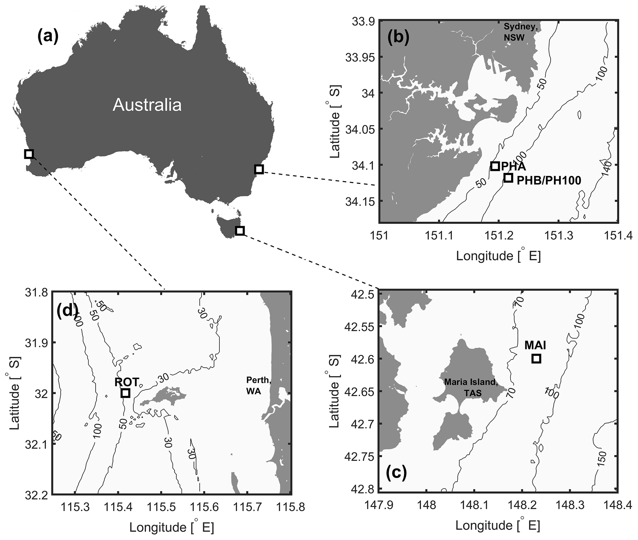
Figure 1 (a) The four long-term oceanographic sampling sites at coastal locations around Australia. (b) The Port Hacking stations (close to Sydney) at approximately 50 and 100 m depth (PHA and PHB/PH100). (c) The Maria Island (Tasmania) station at approximately 90 m depth (MAI) and (d) Rottnest Island (close to Perth, Western Australia) at approximately 55 m depth (ROT). Isobaths (using data from the General Bathymetric Chart of the Oceans (GEBCO), GEBCO Bathymetric Compilation Group, 2023) are also plotted in panels (b), (c) and (d).

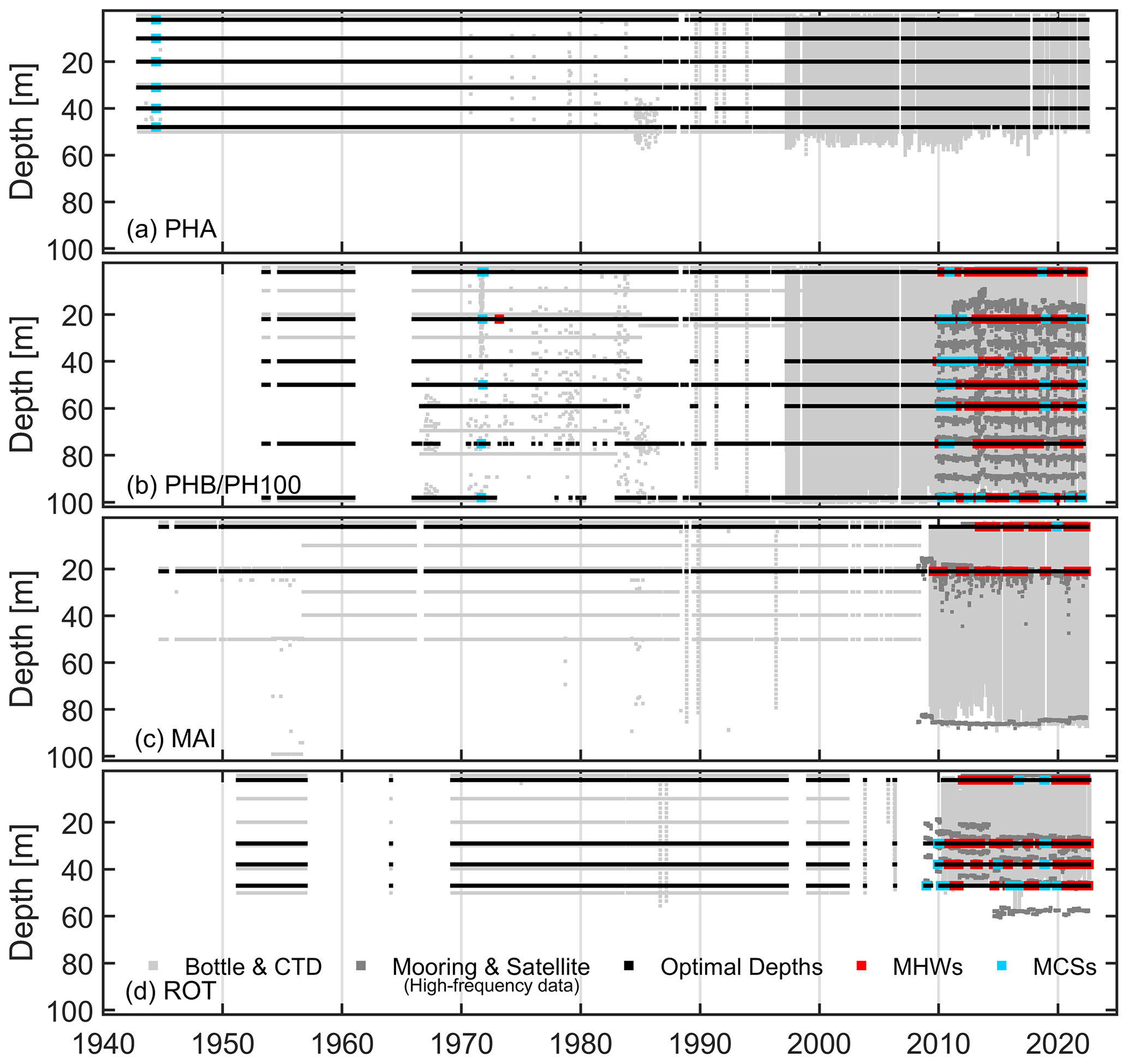
Figure 2 Depiction of available temperature data from bottle and CTD profiles (light grey), high-frequency mooring and satellite data (dark grey) and data binned at optimal depths (black) for the (a) PHA, (b) PHB/PH100, (c) MAI and (d) ROT sites. Data points associated with marine cold spells (MCSs, light blue) and marine heatwaves (MHWs, red) are also shown and in most cases highlight time periods when high-frequency data exist at the sites.

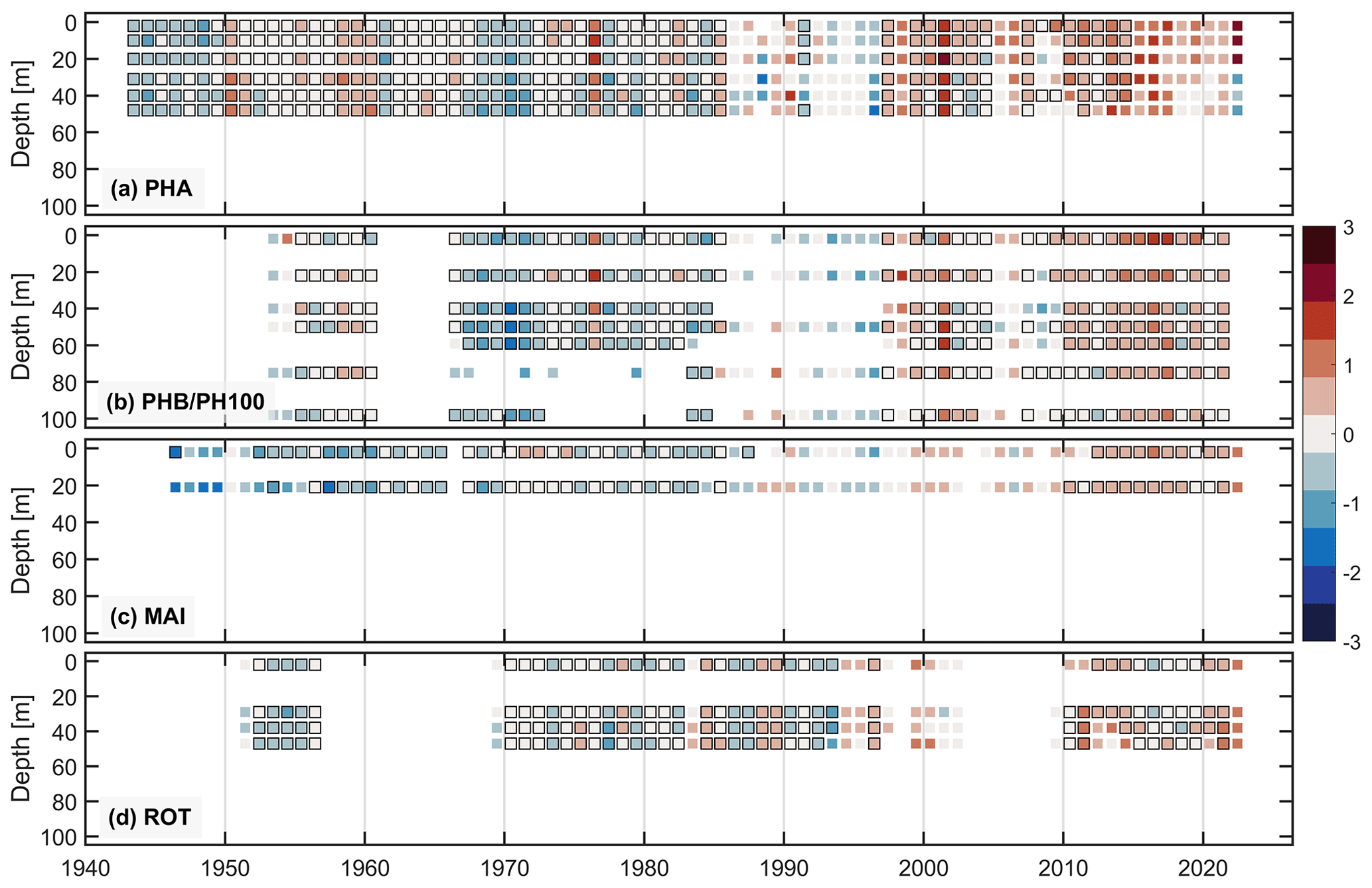
Figure 3 Annual median temperature anomalies relative to the mean daily varying climatology at optimal depths for the (a) PHA, (b) PHB/PH100, (c) MAI and (d) ROT sites. All the years and depths shown have measurements available in at least 4 months of the year, while those years and depths with a solid black outline have measurements available in at least 10 months of the year.

3 The data products

3.1 Multi-decadal time series data products

We build on recently released aggregated multi-decadal ocean temperature time series products at the four oceanographic sites (Roughan et al., 2022a, b), which we refer to as the Australian Multi-Decadal Ocean Time Series (AMDOT) data products. The AMDOT data products at PHA, PHB/PH100, MAI and ROT include multiple-depth ship-based temperatures from bottle samples and electronic CTD sensor profiles. Several different SeaBird Electronics CTD sensors (e.g. SBE17+, SBE19+ or SBE25) have been used to measure temperature and pressure at the sites.

In addition, the aggregated AMDOT data products at sites PHB/PH100, MAI and ROT contain multiple-depth moored temperature measurements. At PHB/PH100, thermistors (Aquatech AQUAloggers 520T or 520PT) were mounted on a mooring line at 8 m intervals through the water column. At approximately 15 to 24 m a Wetlabs water quality meter (WQM) was deployed between 2010 and 2017, which was later replaced by a SeaBird SBE37 (including a second one approximately 6 m above the bottom). At MAI Wetlabs WQMs and SeaBird SBE37s were mounted on a mooring line at around 20 to 25 m and close to the bottom (approximately 90 m). At ROT various temperature sensors (e.g. Wetlabs WQMs, Seabird SBE37 or SBE39) were placed on a mooring line at approximately 22, 27, 35, 43 and 55 m depths (varying over time). More information on these configurations can be obtained from Lynch et al. (2014), Chen and Feng (2021) and Roughan et al. (2022a).

At sites PHB/PH100, MAI and ROT at the surface (0.2 m) after 2012, we include remotely sensed sea surface temperature (SST) data from the IMOS Multi-sensor night-time gridded Super-Collated (L3S) SST data composites (Govekar et al., 2022). We use SST at a drifting buoy depth (approximately 0.2 m, calculated by adding 0.17 K to skin SST; Govekar et al., 2022) that has had the sensor-specific error statistics (SSES) bias removed from each grid cell. Further, we only use SST associated with “quality level” flags ≥4 (less likely to be contaminated by clouds). A full description of the data quality control (QC) and how these aggregated data products were created is provided by Roughan et al. (2022a), and further information specifically on the SST data and methods is provided by Govekar et al. (2022).

Data availability (Table 1 and Fig. 2) is consistent through the water column at PHA because the temperature record consists of bottle and CTD profiles only. However, at PHB/PH100, MAI and ROT, there is increased sub-surface data availability relative to the surface. This is because the satellite-derived SST data that we use start in 2012 and have some gaps (dependent on clear skies).

The annual median temperatures for each site are shown in Fig. 3. The long-term consistency of the temperature data has been tested through comparisons of measurements overlapping in time and space. At PHB/PH100 and MAI, satellite SST agrees well with surface buoy temperature (Hemming, 2023a). At PHB/PH100 there is also good agreement between satellite SST and the nearest sub-surface mooring temperature (Roughan et al., 2022a; Malan et al., 2021) and between water sample and CTD sensor profiles (Hemming, 2023a).

To produce statistics through the water column, we use aggregated temperature data at optimal depth levels to identify temperature extremes. These optimal depth levels (listed in Table 1 for each site and shown in Fig. 2) were selected based on the vertical distribution of the data, similar to the method by Roughan et al. (2022a) to produce daily climatologies.

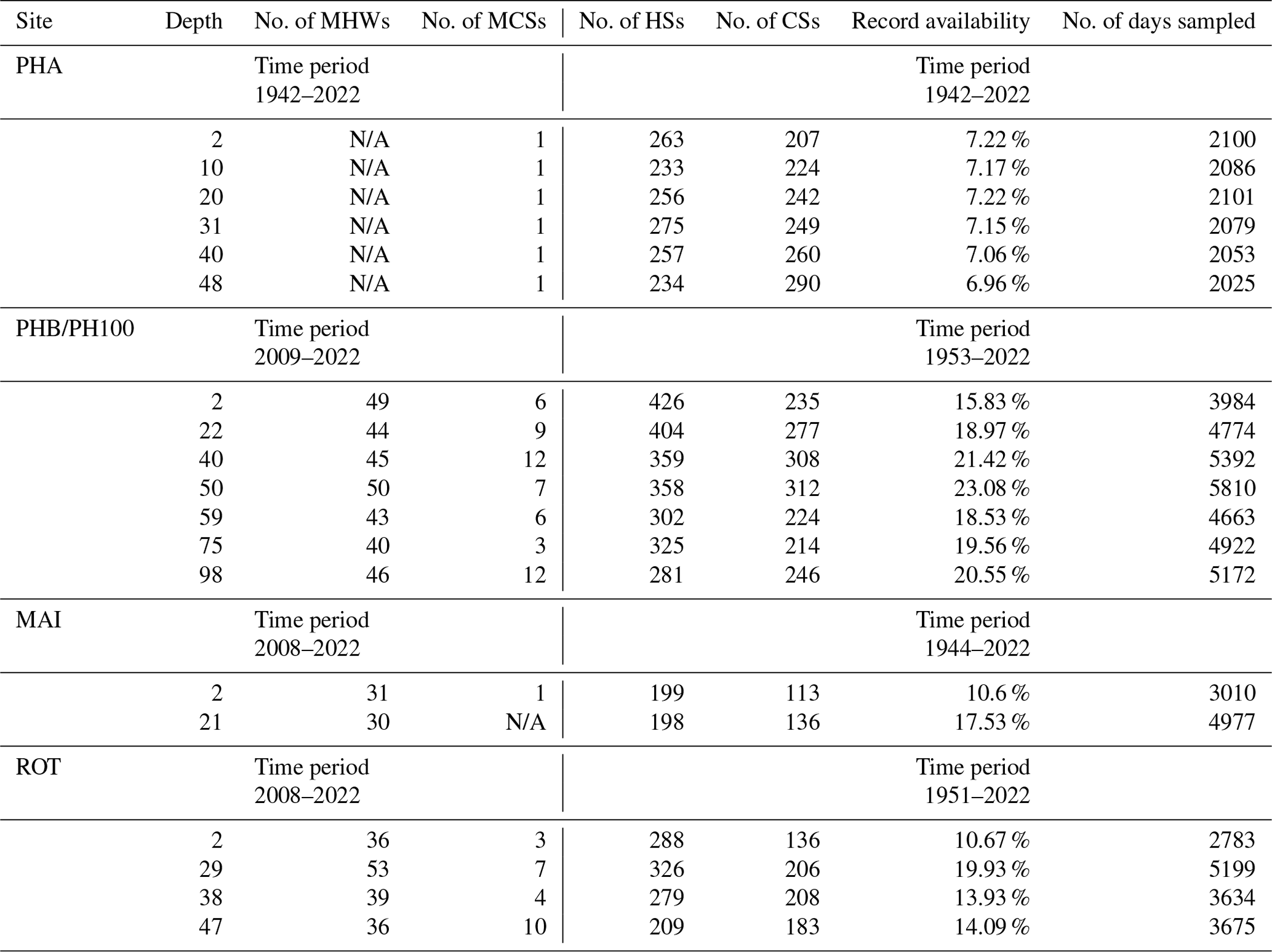
Table 1 Table showing the number of marine heatwaves (MHWs), marine cold spells (MCSs), heat spikes (HSs) and cold spikes (CSs) identified at the Port Hacking 50 and 100 m (PHA and PHB/PH100, respectively), Maria Island (MAI) and Rottnest Island (ROT) sites at multiple depths. HSs and CSs include days when temperatures were higher than the 90th percentile and lower than the 10th percentile, respectively, and do not include days identified during MHWs and MCSs. The time period when we have high-frequency data and hence when we have the most MHWs and MCSs is shown separately from the time period used to additionally detect HSs and CSs. The total record available (excluding interpolated temperatures) at multiple depths as a percentage of the time period between the first and last sampled temperatures is listed for each site. The unique number of days (or daily binned data points) excluding interpolated temperatures available over the site's record (e.g. between 1951 and 2022 at ROT) is also shown (number of days sampled). Here “N/A” denotes where no MHWs/MCSs were detected. At PHA, this is because daily temperatures are not available.

3.2 Deriving extreme temperature event statistics

The method of deriving extreme temperature event statistics are summarised in the flow chart in Fig. 4. We use the open-source Python MHW software package (Oliver, 2020) that uses the widely adopted definitions (Hobday et al., 2016; Schlegel et al., 2021) for deriving MHWs and MCSs relative to a baseline climatology. However, instead of producing new daily climatologies using this MHW software package, we adapted the code to use the daily temperature climatologies produced by Roughan et al. (2022a), who used the method described by Hemming et al. (2020) as input for detecting extreme temperature events. These daily temperature climatologies (Roughan et al., 2022b) at the four coastal sites are derived from the aggregated temperatures used here and described in Sect. 3.1. The climatologies were created for each day of the year (1 January until 31 December, excluding 29 February during leap years) using temperature data within a time-centred moving window of 11 d. To limit warm bias arising from over-representation of mooring data points relative to bottle samples, a bottle-to-mooring ratio was used. The climatologies have been further smoothed using a moving average window of 31 d following the recommendation of Hobday et al. (2016). As the climatologies are provided at regular 10 m intervals between the shallowest and deepest depths, for the purpose of extreme temperature identification, we interpolated the climatology statistics back to optimal depth levels. The reader is referred to Roughan et al. (2022a) for further details on how these daily climatologies were produced.

We identify HSs as temperatures that are higher than the daily varying 90th percentiles and CSs as temperatures that are lower than the daily varying 10th percentiles. When daily binned high-frequency fixed time series are available (after 2008/2009; see Table 1), we further consider MHWs and MCSs when the spikes last for 5 or more consecutive days (as per the widely adopted definition, where a MHW/MCS event needs to last more than 5 d). As suggested by Hobday et al. (2016), we ignore intermittent periods of 2 d or less when temperature extremes ease if followed by another MHW/MCS event. These intermittent periods are identified using daily binned temperatures centred at 12:00 UTC, and hence periods of 2 d or less are represented by one less anomalous daily binned temperature. To increase data coverage, gaps of 2 d or less are filled using linear interpolation prior to detecting MHWs and MCSs using the MHW software package (Oliver, 2020).

The number of extreme temperature events that we detect depends on the site, depth and data availability (Table 1, Fig. 2). Between 198 and 426 HSs and between 113 and 312 CSs were detected when considering all the sites and depths. When considering individual depths, ROT had the most (53) MHWs at a depth of 29 m and MAI had the least (30) at a depth of 21 m. PHB/PH100 had the most MCSs (12) at depths of 40 and 98 m. Only one MCS was detected at MAI at 2 m depth. It was generally not possible to detect MHWs and MCSs at PHA using the Hobday et al. (2016) definition because we only have data that were collected weekly to monthly. However, one MCS was detected at multiple depths in late May and June 1944, when five bottle profiles were collected within a period of 8 d.

The Australian Multi-Decadal Ocean Time Series EXTreme (AMDOT-EXT) data products contain extreme events that sometimes vary over depth. For example, event start and end dates and their category can vary as a function of depth (Fig. 5). This is partially because data availability over time is often non-uniform through the water column, but also because the depth structure of MHW events can vary due to ocean dynamics. For example, in the coastal Sydney region, Schaeffer et al. (2023) showed that MHWs can be shallow, can extend across the whole water column or can be sub-surface only. During atmospherically forced shallow MHWs, for instance, we might expect there to be fewer days when temperatures exceed the 90th percentile at depths below the mixed-layer depth when compared with temperatures at the surface (Schaeffer et al., 2023).

3.3 Data products and variables

We provide one data product at each of the four sites that contains extreme temperature event information, the temperature data used and climatology statistics. We refer to these data products as the AMDOT-EXT data products. Two temperature variables are included in the AMDOT-EXT files: each temperature variable includes the daily binned temperatures at each depth level (±3 m bins). However, one temperature variable has gaps of ≤2 d filled. This latter gap-filled temperature variable was used for detecting extreme temperature events. The AMDOT-EXT data products also include the corresponding time and depth (constant over time) and the climatological mean, 10th and 90th percentiles. Table 2 summarises the names of the variables contained in the AMDOT-EXT files. Event information (e.g. event number, duration or intensity) is accessible using matrix variables with dimensions “TIME” and “DEPTH”. These matrices have the same dimensions as the temperature data and climatology parameters.

The individual MHW and MCS event numbers and the categories defined by Hobday et al. (2018) and Schlegel et al. (2021) are included in the AMDOT-EXT files, with their variable names listed in Table 2. The MHW/MCS category is presented as flags from one to four representing in order “Moderate”, “Strong”, “Severe” or “Extreme” events. Due to the inconsistencies in data sampling over depth and/or regional dynamics, an extreme temperature event may be detected at one depth but not at another, or the length of an event may vary (Fig. 5). Hence, the user should keep in mind that there may be inconsistent event numbers and timings of such events when analysing a particular event over depth.

The AMDOT-EXT data products contain an extreme temperature index variable (TEMP_EXTREME_INDEX) that is useful for identifying the type of extreme temperature event: CS (flag 1), MCS (flag 2), HS (flag 11) and MHW (flag 12). For MHWs and MCSs, we also provide the mean, maximum and cumulative intensities, variance of intensity, and event onset and decline rates. The intensity is the temperature anomaly relative to the chosen statistic (e.g. mean climatology) (Hobday et al., 2016). Over the duration of a MHW/MCS, the cumulative intensity is the sum of the daily temperature intensities, while the variance of intensity is the variation (Hobday et al., 2016). We provide event intensity variables that are relative to both the mean and threshold (e.g. 90th percentile) climatology (see Table 2). The onset rate represents the temperature change rate from the start of a MHW/MCS to the maximum intensity (lowest value for MCSs), while the decline rate represents the temperature change rate from the maximum intensity to the end of the MHW/MCS (Hobday et al., 2016). These metrics are calculated using the MHW software package (Oliver, 2020) according to the methodology described by Hobday et al. (2016) and detailed in their Table 2.

Some metrics for MHWs and MCSs, such as duration, maximum intensity and cumulative intensity, are constant over the duration of an event. In the NetCDF files these constant metrics are repeated for each day of an event. For example, a MHW lasting 6 d with a maximum intensity of 23.2 ^∘C will have six repeated duration values (e.g. 6, 6, 6, 6, 6, 6) and six repeated maximum intensity values (e.g. 23.2, 23.2, 23.2, 23.2, 23.2, 23.2) representing each date of the MHW.

In addition to the AMDOT-EXT NetCDF data products, we provide comma-separated value (CSV) files containing all of the MHW and MCS event information and characteristics at each of the four sites. Please see Appendix A1 for details on how to cite the AMDOT-EXT data products and the CSV files. Tutorials written in Python, MATLAB and R demonstrating how to load and use these data products are available at Zenodo (Hemming, 2024) and are described in Appendices A2 and A3.

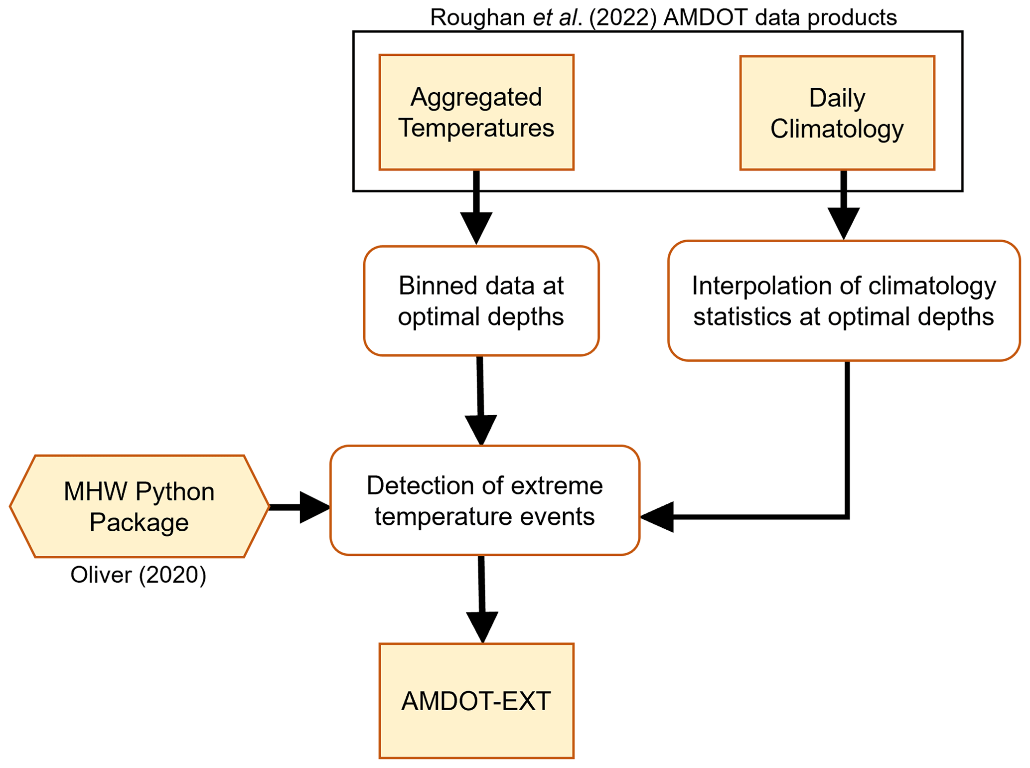
Figure 4 A flow chart showing the process of creating the Australian Multi-Decadal Ocean Time Series EXTreme (AMDOT-EXT) data products.

(Roughan et al., 2022a)Roughan et al. (2022a)Roughan et al. (2022a)Roughan et al. (2022a)Roughan et al. (2022a)(Roughan et al., 2022a)(Roughan et al., 2022a)

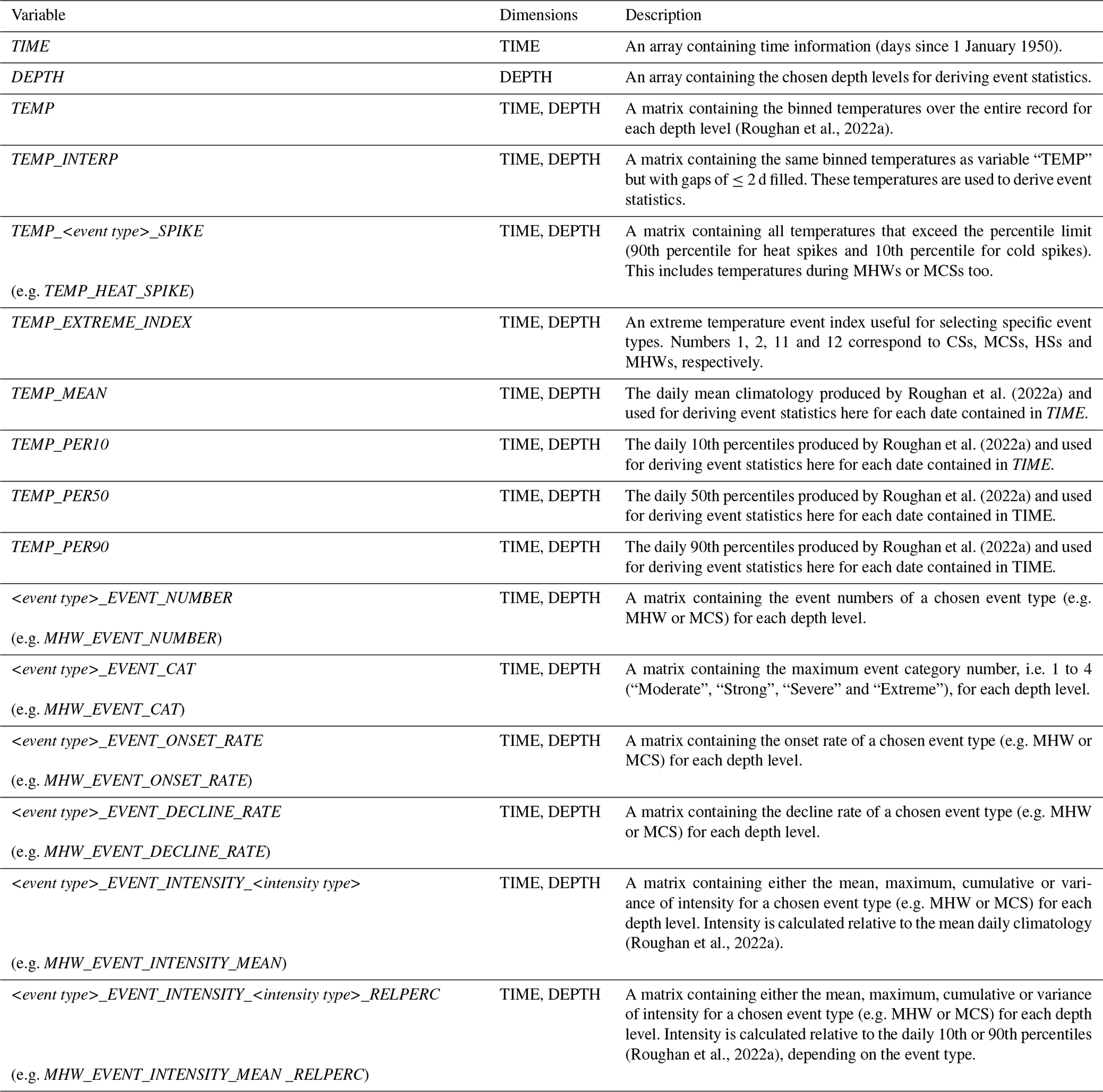
Table 2 A table summarising the variables and their dimensions contained in each AMDOT-EXT NetCDF file with a corresponding description.

3.4 Effects of data availability and the choice of baseline

It is important to consider data availability and the daily climatologies that were used when detecting and discussing extreme temperature events. Sub-surface measurements used at PHA, PHB/PH100, MAI and ROT consist of water samples, electronic CTD sensor profiles and, at PHB/PH100, MAI and ROT, mooring data. Data availability over time and in space can be seen in Figs. 2 and 3, with notable gaps at PHB/PH100 between the 1960s and 1990s and at ROT during the 1950s, 1960s and 2000s. Temperature data availability over depth relative to the surface is also shown in Table 1. Additionally, the depths at which samples were taken have changed with time, which presents a challenge when it comes to detecting extreme sub-surface temperature events. We partially deal with this by filling gaps of ≤2 d. However, there are many instances of gaps >2 d (Figs. 2 and 3).

We use daily climatology thresholds incorporating temperature data over the entire record, which is between 70 and 81 years at the four sites. We acknowledge that using a climatology of approximately 30 years is recommended (Hobday et al., 2016; WMO, 2018) and is commonly used for surface MHW studies (e.g. Frölicher et al., 2018; Oliver et al., 2018; Elzahaby and Schaeffer, 2019), where such data exist. Schlegel et al. (2019) showed that using a climatology period >30 years may affect MHW detection in a similar way to using a climatology period <30 years, dependent on environmental multi-decadal variability. Further, Rosselló et al. (2023) highlight the impact of long-term trends on MHWs and argue that a moving baseline is more adequate for detecting consistently rare extremes, although presently there is much debate on this subject (Amaya et al., 2023; Sen Gupta, 2023). We use daily climatologies calculated using the entire temperature record at the long-term sites because 30-year daily sub-surface datasets do not exist yet at our chosen sites. Temperatures at two of the sites, PHB/PH100 and MAI, have increased non-linearly over time, with mean temperatures (dependent on depth) in 2022 approximately 0.5 to 1.3 ^∘C warmer on average relative to the 1940 and 1950s (Hemming et al., 2023), and annual median temperature anomalies can be seen in Fig. 3. Presently, high-frequency sub-surface data at the four sites only extend back approximately 13 to 14 years. We acknowledge that the number of extreme temperature events and their metrics will differ in the future when a 30-year daily climatology becomes available and that it will vary depending on which 30-year period is used (as suggested by Schlegel et al., 2019).

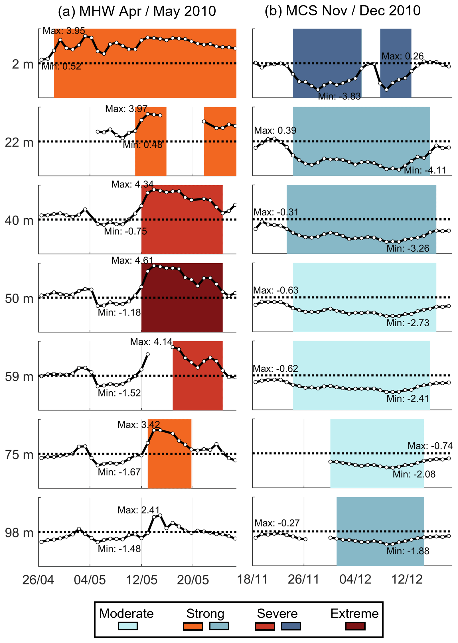
Figure 5 Examples of a MHW and MCS over depth at the PHB/PH100 site: (a) MHW in April and May 2010 and (b) MCS in November and December 2010. The daily varying temperature anomalies (^∘C) relative to the mean (black line with white dots) are shown for each depth. Time periods when MHWs or MCSs occur are shaded, with colours indicating the category (“Moderate”, “Strong”, “Severe” and “Extreme”) as shown in the legend. The maximum and minimum temperature anomaly relative to the mean for each time period and depth is also shown.

4 Usage

The AMDOT-EXT data products described here can be used to analyse extreme ocean temperature events at the four sites at depths through the water column over time. For example, the MHW_EVENT_CAT variable could be used to select “Strong” MHWs at a particular depth and site. Applying this information to variables TIME and MHW_INTENSITY_MEAN would select the timings and mean intensities of “Strong” MHWs. Further, exporting the data during such events might be useful for working with other datasets, e.g. phytoplankton data for investigating the biological impact of MHWs. Code written in Python, MATLAB and R demonstrating how to load and slice the AMDOT-EXT data products is available at Zenodo (Hemming, 2024), and further details are provided in Appendices A2 and A3.

5 Marine heatwaves and cold spells

As shown in Table 1, MHWs and MCSs were most often detected at sites and depths that had high-frequency temperature data (typically between 2008/2009 and 2022). In Fig. 6 we explore the most intense events (chosen based on cumulative intensity) between 2008/2009 and 2022 at the long-term sites PHB/PH100, MAI and ROT. The most intense MHWs were at approximately 20 m depth at sites PHB/PH100 and MAI in 2015 and 2015/16, respectively (Fig. 6a and b). These coastal events coincided with the far-reaching MHW conditions in the Tasman Sea related to the EAC (Oliver et al., 2017). At ROT the most intense MHW between 2008 and 2022 was at 29 m in 2011 (Fig. 6c) at the time of the well-documented Ningaloo La Niña MHW (Feng et al., 2013; Wernberg et al., 2013; Pearce and Feng, 2013). On average, the intensity of the 2015 MHW at PHB/PH100 was 2.4 ^∘C above the mean climatology and lasted 50 d, while the MAI and ROT MHWs were on average 2.2 and 1.9 ^∘C above the mean climatology and lasted 151 and 60 d, respectively.

The most intense MCSs between 2008/2009 and 2022 were in 2010 and 2015 at PHB/PH100 and ROT, respectively (Fig. 6d and f). At PHB/PH100 and ROT, these events were 3.1 and 1.8 ^∘C cooler than the mean climatology on average and lasted 22 and 25 d, respectively. At MAI we detected one MCS between 2008 and 2022 lasting 5 d in late 2019 which was 1.6 ^∘C cooler than the mean climatology on average.

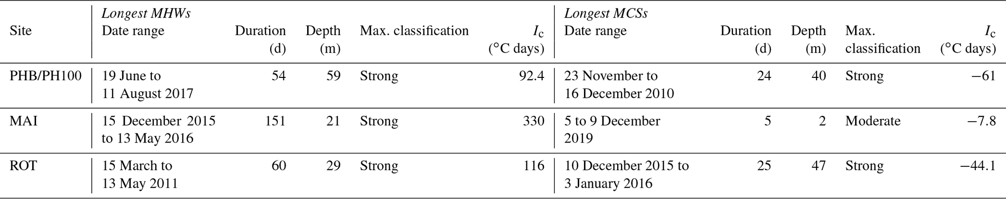
Information relating to the longest MHWs between 2008/2009 and 2022 at sites PHB/PH100, MAI and ROT is provided in Table 3. The longest MHW detected lasted 151 d at MAI (same as in Fig. 6b) between 15 December 2015 and 13 May 2016, while the longest MHWs at PHB/PH100 and ROT lasted 54 and 60 d, respectively. The longest ROT MHW was also the most intense, as described above and shown in Fig. 6c. The cumulative intensities of these MHWs were between 92.4 and 330 ^∘C days. The longest MCSs between 2008/2009 and 2022 lasted 24 and 25 d in 2010 and 2015/2016 at PHB/PH100 and ROT, respectively, and just 5 d in 2019 for a single MCS at MAI as described above. The cumulative intensities at PHB/PH100 and ROT for these MCSs were −61 and −44.1 ^∘C days, respectively. The MAI MCS had a cumulative intensity of −7.8 ^∘C days. Almost all of the longest MHWs and MCSs were classified as a “Strong” event and occurred below the surface.

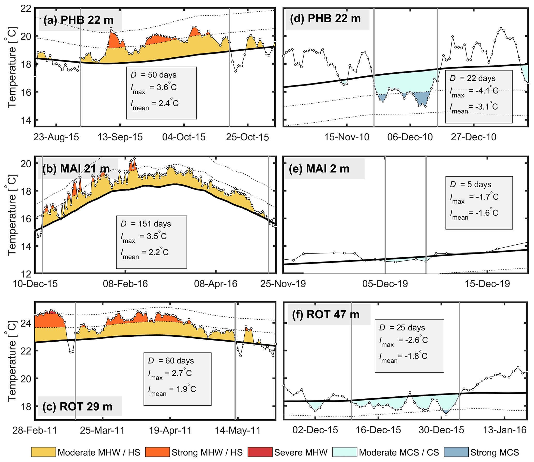
Figure 6 Examples of (a)–(c) MHWs/HSs and (d)–(f) MCSs/CSs, with the maximum cumulative intensity at the long-term sites PHB/PH100, MAI and ROT. The area underneath the portion of the time series experiencing an extreme event is filled according to the categories “Moderate MHW/HS” (yellow), “Strong MHW/HS” (orange), “Severe MHW” (red), “Moderate MCS/CS” (light blue) and “Strong MCS” (dark blue). The metrics shown are duration (“D”), maximum intensity (“I_max”) and mean intensity (“I_mean”). The time period of each MHW or MCS is indicated by vertical grey lines. Each panel covers a different time period, and hence the x limits are not the same in each panel.

Table 3 The date range, duration, depth, maximum classification and cumulative intensity (I_c) for the longest MHWs and MCSs at sites PHB/PH100, MAI and ROT.

6 Code and data availability

The AMDOT-EXT data products are available as NetCDF files (https://doi.org/10.26198/wbc7-8h24, Hemming et al., 2024), and variables contained in the NetCDF files are listed in Table 2. The summary CSV files are available here: https://doi.org/10.26198/wbc7-8h24. Any and all use of the AMDOT-EXT data products provided here must include a citation (see Appendix A1). Any updated data products and/or potential new products (e.g. at other sites or using other ocean variables) will be hosted at the same location. Therefore, it is advisable that data users seek the latest data product version.

We provide basic scripts in MATLAB, Python and R demonstrating how to download and load the data products, use the NetCDF variables, and export the data as CSV files. These scripts are available online at Zenodo (Hemming, 2024) and are available to use under a Creative Commons Attribution 4.0 International license (CC BY 4.0). Please see Appendix A below for more details.

7 Summary

Extreme temperature events have been identified and characterised at multiple depths between the surface and the bottom at four oceanographic sites: PHA, PHB/PH100, MAI and ROT using long-term ocean temperature records. We provide four data products – one data product per oceanographic site – including indices for identifying extreme temperature events, their characteristics as well as corresponding temperature time series and daily climatology statistics. We refer to these new data products as the Australian Multi-Decadal Ocean Time Series EXTreme (AMDOT-EXT) data products.

These AMDOT-EXT data products are freely accessible at the Australia Ocean Data Network thredds server, and we provide code tutorials in Appendix A demonstrating how to load the data products, use the NetCDF variables and export the data as CSV files. We also provide CSV files containing all of the MHW and MCS event information and characteristics at each of the four sites. Refer to the Code and data availability section for information on how to access the NetCDF and CSV files.

Using the AMDOT-EXT data products, we compare the number of extreme temperature events at the four sites and explore the most intense and longest MHWs and MCSs, which were often below the surface. These data products can be used to characterise and assess the impacts of MHWs and MCSs in coastal waters around Australia.

The AMDOT-EXT data products highlight the challenges faced when detecting extreme temperature events using sporadic long time series. Hence, it is vital that high-temporal-resolution measurements at multiple depths (i.e. moored thermistor data) continue into the future to fully understand extreme temperature events and their variability in the face of rapid environmental change.

Appendix A: User guide and tutorials

A1 Citing the AMDOT-EXT data products

Any and all use of the AMDOT-EXT data products or accompanying event summary CSV files described here must include the following.

• A citation to this paper

• A reference to the data citation as written in the NetCDF file attributes

• The following acknowledgement statement: “Data were sourced from Australia's Integrated Marine Observing System (IMOS) – IMOS is enabled by the National Collaborative Research Infrastructure Strategy (NCRIS).”

A2 Loading AMDOT-EXT data products and saving them as CSV files

The tutorial script “get_DataProducts” available at Zenodo (Hemming, 2024) demonstrates how to do the following.

• Load the MAI AMDOT-EXT data product using OPeNDAP.

• Select data during a MHW event.

• Export the data as a CSV file.

A version of this tutorial is available for use with R, Python and MATLAB and can be modified to use any AMDOT-EXT data product.

A3 Slicing AMDOT-EXT data product variables based on event characteristics

The tutorial script “slice_DataProducts” available at Zenodo (Hemming, 2024) demonstrates how to do the following.

• Load the PH100 AMDOT-EXT data product using OPeNDAP.

• Select data during “Strong” category MHWs at a depth of 22 m.

• Calculate and display mean characteristics during “Strong” category MHWs at this depth.

• Save the sliced dataset as either a NetCDF, MAT (MATLAB) or rdata (R) file, as well as a CSV file.

A version of this tutorial is available for use with R, Python and MATLAB and can be modified to slice any AMDOT-EXT data product based on any event characteristic.