A decade of marine inorganic carbon chemistry observations in the northern Gulf of Alaska – insights into an environment in transition

As elsewhere in the global ocean, the Gulf of Alaska is experiencing the rapid onset of ocean acidification (OA) driven by oceanic absorption of anthropogenic emissions of carbon dioxide from the atmosphere. In support of OA research and monitoring, we present here a data product of marine inorganic carbon chemistry parameters measured from seawater samples taken during biannual cruises between 2008 and 2017 in the northern Gulf of Alaska. Samples were collected each May and September over the 10 year period using a conductivity, temperature, depth (CTD) profiler coupled with a Niskin bottle rosette at stations including a long-term hydrographic survey transect known as the Gulf of Alaska (GAK) Line. This dataset includes discrete seawater measurements such as dissolved inorganic carbon and total alkalinity, which allows the calculation of other marine carbon parameters, including carbonate mineral saturation states, carbon dioxide (CO₂), and pH. Cumulative daily Bakun upwelling indices illustrate the pattern of downwelling in the northern Gulf of Alaska, with a period of relaxation spanning between the May and September cruises. The observed time and space variability impart challenges for disentangling the OA signal despite this dataset spanning a decade. However, this data product greatly enhances our understanding of seasonal and interannual variability in the marine inorganic carbon system parameters. The product can also aid in the ground truthing of biogeochemical models, refining estimates of sea–air CO₂ exchange, and determining appropriate CO₂ parameter ranges for experiments targeting potentially vulnerable species. Data are available at https://doi.org/10.25921/x9sg-9b08 (Monacci et al., 2023).

1 Introduction

During the last decade, OA has emerged as one of the most prominent topics in marine research and understanding its potential impacts could be vital for the sustainable management of ecosystem services around the world. The global oceans have become progressively acidified (e.g., Feely et al., 2004, 2009; Jiang et al., 2019) over the last two and half centuries as they have taken up approximately one–fourth of the human output of CO₂ into Earth's atmosphere (e.g., Sabine and Tanhua, 2010; Friedlingstein et al., 2022). At present, the decrease in the average global surface ocean pH averages ∼0.1 units, making surface ocean acidity 30 % higher than at the start of the Industrial Revolution (Gruber et al., 2023; Jiang et al., 2019). This decline in ocean pH and the sharp rise in seawater carbon dioxide (CO₂) has led to broad reductions in carbonate mineral concentrations in the oceans with diverse but often detrimental consequences for both pelagic and benthic species (Andrade et al., 2018; Barton et al., 2012; Bechmann et al., 2011; Cooley and Doney, 2009; Hurst et al., 2012, 2013, 2019; Long et al., 2013; Wright-LaGreca et al., 2022).

Although acidification is a global phenomenon in the open ocean, there are regional hotspots where natural coastal processes can precondition waters to have lower pH and saturation states for carbonate minerals aragonite and calcite (Ω_A and Ω_C respectively), creating additive vulnerabilities. Regions where OA is amplified by concurring anthropogenic and natural processes are also interacting with changing temperature, salinity, and gas solubility (Feely et al., 2018). This is particularly true in the high-latitude north Pacific Ocean (e.g., Byrne et al., 2010; Dore et al., 2009), where studies have shown that the region is already experiencing seasonal events in which carbonate minerals, such as the biologically important aragonite, can become undersaturated (Evans and Mathis, 2013; Evans et al., 2013, 2014). Models project that under current emission rates large areas of the subarctic Pacific could become undersaturated with respect to aragonite (Ω_A<1) by as early as mid-century and the entire region will be perennially undersaturated by 2100 (e.g., Gruber et al., 2023; Mathis et al., 2015). The seasonal effects of glacial runoff may also intensify acidification processes because these waters may have naturally low carbonate mineral concentrations depending on how they are discharged into the marine environment (Evans et al., 2014; Reisdorph and Mathis, 2014). Consequently, high-latitude regions provide a real-time laboratory for the evaluation of potential impacts on organisms, and the associated marine resources that they provide (Mathis et al., 2015).

The northern Gulf of Alaska (NGA) is a predominantly downwelling system (Royer and Emery, 1987) with seasonal exceptions. When the onshore surface Ekman transport relaxes in the summer, deep, nutrient-rich, cold water can inundate the continental shelf below the surface layer near the shore (Weingartner et al., 2005). The new intermediate water, also enriched in CO₂, causes the saturation horizon for both aragonite and calcite minerals to shoal to within 100 and 250 m from the surface respectively (Feely et al., 2004). Along the West Coast of North America, intense wind-driven upwelling can cause the saturation horizon to shoal to the surface over the continental shelf, leaving large, inshore areas exposed to conditions that have been shown to be corrosive to some calcifiers (Bednaršek et al., 2012, 2014; Comeau et al., 2010). The phenomenon was first observed in the California Current System (Feely et al., 2008), but has also been observed in other high-latitude regions (e.g., Bednaršek et al., 2012; Mathis et al., 2012).

The NGA supports a diverse ecosystem that includes some of the largest commercial fisheries in the world and serves as a pathway for biogeochemical preconditioning of the Bering Sea and Pacific–Arctic region (Cross et al., 2018). The Bering Sea region, like the NGA, supports a highly productive system and these two large marine ecosystems support the largest single-species fishery in the world, walleye pollock (Fissel et al., 2021). On the relatively shallow (<60 m) Bering Sea shelf, there is a natural coupling between surface and bottom waters that is driven by the primary production and respiration signals of large phytoplankton blooms (Mathis et al., 2011a, b, 2014). This leads to bottom water conditions where Ω_A<1 for months at a time, and localized retention of CO₂ can lead to calcite undersaturation (Ω_C<1; Cross et al., 2013).

When all these factors are considered, it becomes obvious that the NGA is at a critical intersection point for coastally driven OA processes. This issue is of particular importance for the people that rely on marine resources. Alongside these natural vulnerabilities, anthropogenic perturbations may cause ecosystem-level shifts that have the potential to decrease the economic value of commercial fisheries. More than 60 % of the catch by weight of US fisheries are from Alaskan waters (NMFS, 2022) and impacts on commercial and subsistence fishing are equally important topics in conversations on marine resources in Alaska (Frisch et al., 2015; Szymkowiak and Steinkruger, 2023). Many communities, particularly those in the NGA region, are vulnerable to risks associated with OA through the loss of culture, jobs, income, and food security (Mathis et al., 2015). Several economically important species have shown negative effects of OA on various developmental stages (e.g., Hurst et al., 2019; Long et al., 2013). Experiments on the economically critical red king crab fishery led to a population dynamics model to predict potential effects on fishery yield (Punt et al., 2014, 2021) and the economic impacts on Alaska (Seung et al., 2015).

To better understand the processes that influence inorganic carbon chemistry and in turn, OA in the NGA, we assembled this decadal time–series data product. Ocean biogeochemical observations, like those we present in this dataset, help researchers determine biogeochemical model performance (e.g., Hauri et al., 2020; Siedlecki et al., 2017), calculate sea–air CO₂ flux (e.g., Evans et al., 2013; Gruber et al., 2023), and set ranges to determine physiological responses to OA on specific species (e.g., Hurst et al., 2013; Long et al., 2013). In turn, these applications can aid in understanding cascading societal impacts of changes in the marine carbonate system, such as determining the vulnerability of a region's marine resources or the effectiveness of marine carbon dioxide removal. We show how mean water column structure and circulation patterns impact variability in carbon chemistry, discuss some long-term changes in carbon chemistry parameters, and assess the drivers contributing to these patterns of variability as examples of how this data product may be used. In general, we find a pattern of decreasing surface CO₂ during the spring season over time. Although our data suggest that this temporal shift might be unrelated to temperature patterns, additional research is required to document a hypothesized change in the timing or magnitude of the spring bloom that could be leading to these changes. In general, we find that this dataset is good for exploring natural environmental variability in the physical system, and the impacts on carbon parameters.

2 Methods

2.1 Study Area

The GAK Line (Fig. 1) is a long-term oceanographic time series that has been sampled at least biannually since 1997. The GAK Line is often colloquially referred to as the Seward Line (SL), because the research cruises begin and end from the University of Alaska Fairbanks (UAF) Seward Marine Center in Qutekcak (Seward), Alaska. The SL program began as part of the Northeast Pacific Global Ocean Ecosystem Dynamics (GLOBEC) program, evolved under a funding consortium from 2005–2017, and is currently part of the Northern Gulf of Alaska Long Term Ecological Research (NGA–LTER) project. The northernmost station, GAK1, is at the mouth of Resurrection Bay, with major stations spaced ∼20 km apart across the continental shelf to GAK15. In addition to visiting the major stations, most cruises in this dataset began at an inner station, RES2.5, located within Resurrection Bay, and occasionally visited the intermediate (i) stations, spaced every ∼10 km from GAK1i to GAK9i.

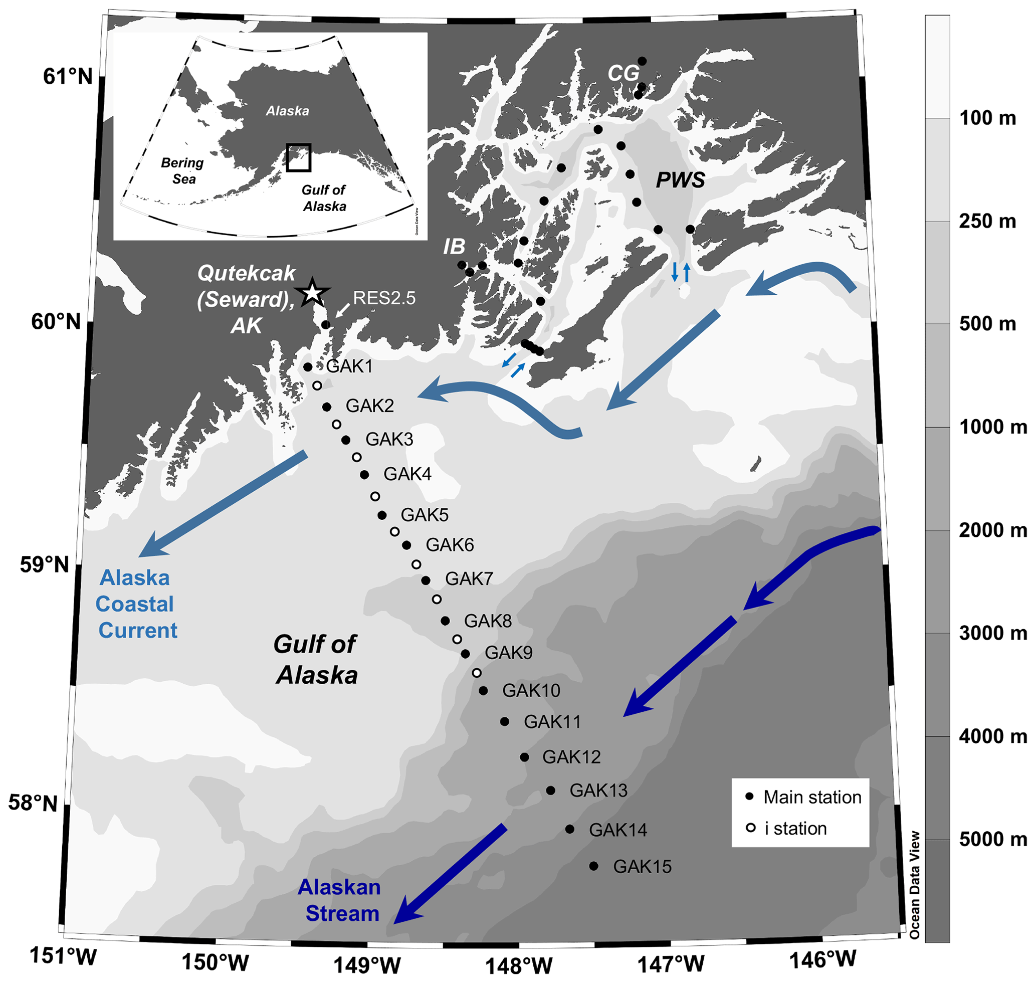
Figure 1 Map and circulation of the study area in the Northern Gulf of Alaska, created using Ocean Data View (Schlitzer, 2022) and adapted from Reed et al. (1987). Main Gulf of Alaska (GAK) Line stations 1–15 are mostly sampled each cruise (filled circles), intermediate (i) stations are sampled periodically (open circles). Cruises begin and end in Qutekcak (Seward), AK, and occur mostly during the months of May and September. Most cruises also sampled repeat stations in western Prince William Sound (PWS) including the glacially influenced stations in Icy Bay (IB) and near the Columbia Glacier (CG). Nearshore stations are defined as GAK1–2, middle stations are GAK3–7, and offshore stations are GAK8–15.

The GAK Line has two dominant westward circulation features: the Alaska Coastal Current (ACC) and the Alaskan Stream (Fig. 1). The ACC hugs the coast and is driven by freshwater discharge (Childers et al., 2005; Reed et al., 1987; Royer, 1975) and the Alaska Stream (AS) flows along the continental slope and is driven by the Alaska Gyre (Ladd et al., 2016; Stabeno et al., 2004; Weingartner et al., 2005). The Alaska Gyre controls the circulation in the Gulf of Alaska basin, which responds to the Aleutian Low pressure system and the Pacific Decadal Oscillation. Strengthened seasonal downwelling over the shelf (Royer and Emery, 1987) results from cyclonic wind stress over the Gulf of Alaska basin from the Aleutian Low. Stronger winds and storms associated with the Aleutian Low are typical in fall, winter, and spring. The resulting downwelling restricts the ACC to a narrow, deep band along the coast (Weingartner et al., 2005) and constructs a shelf break front along the AS (Fig. 2a). Downwelling winds subside in the summer, broadening and shoaling the ACC (Fig. 2b) and allowing a subsurface inflow of cold, nutrient-rich Pacific water onto the shelf (Childers et al., 2005; Weingartner et al., 2005). This seasonal relaxation of downwelling presumably allows for longer on-shelf summer residence time of subsurface water that may experience elevated rates of organic matter respiration fueled by high summertime primary productivity.

Figure 2 Northern Gulf of Alaska shelf flow. (a) Fall, winter, and spring shelf flow characterized by onshore transport and downwelling with a relatively narrow (10–20 km) and deep (200 m) Alaska Coastal Current. (b) Summer shelf flow characterized by a relaxation of downwelling, allowing the deep inflow of Alaska Stream water under a broader (40 km) and shallower (50 m) Alaska Coastal Current (adapted from Shake, 2011).

The Bakun upwelling indices are calculated based on Ekman's theory of mass transport due to wind stress (Bakun, 1973, 1975; Schwing et al., 1996). Positive values of the Bakun upwelling index are, in general, indicative of upwelling, whereas negative values imply downwelling. Relative to other upwelling indices broadly available, the Bakun index uses sea-level pressure fields from an atmospheric reanalysis to derive estimated near-surface winds. Other indices use winds directly from atmospheric reanalysis that assimilate satellite and in situ wind measurements, both of which are limited in the Gulf of Alaska basin. However, there are important limitations to the Bakun product: (1) it does not fully account for upwelling driven by wind stress curl (e.g., upwelling associated with alongshore changes in wind), and (2) it does not account for cross-shore geostrophic transport. Other upwelling indices have been developed for the North American West Coast (e.g., CUTI and BEUTI, Jacox et al., 2018), which resolve some of these challenges, but are not available for this geographic region. To provide context for this dataset, here we show annual cumulative downwelling by plotting the cumulative sum of the Bakun Index values over each year (Fig. 3). Bakun upwelling indices for 60^∘ N were obtained from the NOAA Environmental Research Division website: https://oceanview.pfeg.noaa.gov/products/upwelling/dnld (last access: 2 August 2023). The Cumulative Daily Upwelling Indices (CDUI) for our study area and time show the magnitude and duration of downwelling conditions experienced in the NGA throughout the year with, importantly, a period of relaxation nominally between May and October.

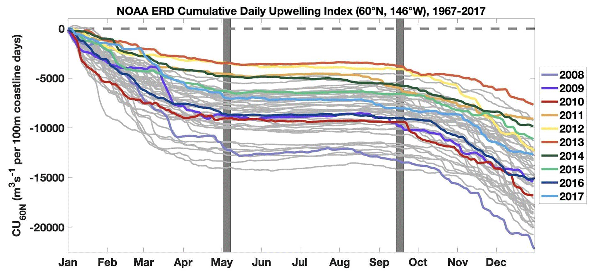
Figure 3 National Oceanic and Atmospheric Administration (NOAA) Environmental Research Division (ERD) Cumulative Daily Upwelling Index at 60^∘ N, 146^∘ W from 1967 to 2017 (adapted from https://oceanview.pfeg.noaa.gov/products/upwelling/intro, last access: 2 August 2023). Negative cumulative (CU) values indicate a downwelling system. Study years (2008–2017, color) are highlighted from the full index years (gray). Average cruise dates in May and September are indicated by shaded, vertical bars.

2.2 Data Collection and Analysis

The biannual cruises in this dataset were typically completed in May and September from 2008 to 2017. Weather, instrumentation, and personnel were the limiting factors to visiting all sampling stations for each cruise. All data presented here were collected using a Seabird 911 Plus conductivity, temperature, and depth (CTD) profiler with a rosette sampler holding twelve 5 L Niskin bottles. A Seabird 43 dissolved oxygen sensor was included for all cruises after Fall 2011 (TXF11). Temperature (T, ITS–90), Salinity (S, PSS–78), and Oxygen (O₂, Tau and hysteresis corrections applied) bottle data presented here were processed from the upcast profiles using Seabird Scientific Seasoft V2 software.

Discrete seawater samples were collected from the Niskin bottles to be analyzed in the laboratory for O₂, dissolved inorganic carbon (DIC), total alkalinity (TA), nutrients (nitrate, nitrite, phosphate, and silicic acid), and stable oxygen isotope ratio (δ¹⁸O) of seawater. When collected, discrete O₂ samples were drawn from the Niskin first, following the GO–SHIP Repeat Hydrography Manual (Langdon, 2010) protocol, and analyzed using the Winkler method (Carpenter, 1965; Winkler, 1888) on a Langdon Amperometric titrator at the Ocean Acidification Research Center (OARC) at UAF.

Following the discrete O₂ collection, discrete seawater samples for DIC and TA were drawn from the Niskin into rinsed, borosilicate glass bottles, fixed with saturated mercuric chloride solution, and sealed until analyzed. All DIC and TA samples were analyzed at the OARC at UAF, but methods vary depending on the years. DIC samples collected from 2008 to 2013 were analyzed by coulometric titration using a Versatile Instrument for the Determination of Total Alkalinity (VINDTA) 3C paired with a UIC Coulometer. DIC samples collected from 2014 to 2017 were analyzed using infrared detection with an Automated InfraRed Inorganic Carbon Analyzer (AIRICA) paired with a LiCOR 7000. TA samples were analyzed in an open cell by potentiometric titration using a VINDTA 3C or 3S. All DIC and TA measurements were routinely calibrated using Certified Reference Materials (CRM) from the Dickson Laboratory at the Scripps Institute of Oceanography. Repeat analyses and comparisons across OARC equipment show that there was no analytical difference across the various instrumentations used; additional discussion on error is included in Sect. 2.4.

Discrete samples for nutrient analyses were collected and analyzed by various laboratories using similar though distinct methods. Samples for nutrient analyses collected during cruises in 2008, 2009, 2010, and 2012 were drawn into rinsed, high-density polyethylene (HDPE) vials, frozen at sea, and analyzed at the Whitledge Laboratory at UAF. Here, samples were thawed immediately prior to analyses using colorimetric techniques on a Technicon AutoAnalyzer II and Alpkem model 300 continuous nutrient analyzers (Childers et al., 2005; Whitledge et al., 1981). Samples for nutrient analyses collected during cruises in 2011 and 2013–2015 were syringe-filtered (using 25 mm, cellulose acetate filters with a 0.45 µm pore size) into HDPE vials, frozen at sea, and analyzed at the National Oceanic and Atmospheric Administration (NOAA) Pacific Marine Environmental Laboratory (PMEL). Here, samples were thawed 3–12 h before analyses according to the methods of Gordon et al. (1993) using a combination of analytical components from Alpkem, Perstorp, and Technicon. Samples for nutrient analyses collected during cruises in 2016 were also filtered using the previously described method but analyzed at OARC at UAF. Here, samples were thawed overnight before being analyzed according to the methods of Gordon et al. (1993) using a SEAL Analytical AA3 continuous flow analyzer. Samples for nutrient analyses collected during cruises in 2017 were filtered and analyzed at the Nutrient Analytical Facility (NAF) at UAF. Here, samples were thawed overnight and brought to room temperature before analyses on a Seal Analytical QuAAtro39 continuous flow analyzer according to the methods of Armstrong et al. (1967) and Murphy and Riley (1962). The data we report here are from four macronutrient variables: nitrate, nitrite, phosphate, and silicate (heretofore silicic acid). Silicate data from cruises in 2011 and 2013–2017 had a second analysis performed the following day (first analyses results are not reported) to avoid low values caused by potential polymerization during frozen storage (Burton et al., 1970; Macdonald et al., 1986; Zhang and Ortner, 1998). We believe that results from the differing methods used by the various laboratories are mostly comparable, including the filtered vs. non–filtered sampling methods, except for the repeat silicate analysis. Additional discussion of the variability in these methods is included below in Sect. 2.4.

Stable oxygen isotope (δ¹⁸O) samples were collected in borosilicate glass vials with no headspace, sealed with parafilm, and submitted to the Stable Isotope Laboratory (SIL) at Oregon State University (OSU). All δ¹⁸O values are reported relative to Vienna Standard Mean Ocean Water (VSMOW).

2.3 Data Organization and Manipulation

This data product merges the GAK Line data from 20 cruise-level archived datasets (Table 1; Monacci et al., 2020a–j) and is organized using best practice data standards including column header abbreviation standards from Jiang et al. (2022; Table 2). A sample identifier (sample ID) is generated to create a value unique to each EXPOCODE to easily incorporate data into data products such as the Coastal Ocean Data Analysis Product in North America (CODAP–NA; Jiang et al., 2021). The sample ID uses the formula outlined by Jiang et al. (2021) and is calculated following Eq. (1):

$$\begin{array}{}\text{(1)}& \begin{array}{rl}\text{Sample ID}=& \text{Station ID}\times \mathrm{10}\mathrm{000}+\text{Cast number}\times \mathrm{100}\\ & +\text{Rosette position}.\end{array}\end{array}$$

Table 1 List of cruises used to produce this data product. EXPOCODE: Expedition code consists of the four-digit International Council for the Exploration of the Sea (ICES) platform code and the date of departure from port (UTC) in YYYYMMDD. Cruise: The project Cruise name, including the letters of the ship (TX = R/V Tiĝlax̂), the northern hemisphere season (S = Spring, F = Fall), and the year in format YY (2008=08). Ship: Vessel name used for field work, where ¹ indicates that the R/V Tiĝlax̂ experienced engine problems and the M/V Island C was chartered in late May to occupy stations GAK2–15, although no DIC/TA samples were collected. Start Date and End Date: UTC in DD/MM/YY. DOI: Digital Object Identifier (Monacci et al., 2020a–j). CRM Batch: Batch numbers of the Certified Reference Materials. TA and DIC: Mean uncertainty of triplicate discrete samples in µmol kg⁻¹. Nutrients: Laboratory where analysis of discrete nutrient samples were analyzed (UAF-WL = University of Alaska Fairbanks Whitledge Lab, PMEL = Pacific Marine Environmental Laboratory, UAF-OARC = UAF Ocean Acidification Research Center, UAF-NAF = UAF Nutrient Analytical Lab), where ² indicates all nutrient values are QF=3 and are not included in this merged data product. O₂, δ¹⁸O, i: Dissolved oxygen, stable oxygen isotope ratio, and GAK Line i stations, where × indicates that data were collected. All files include data with variables CTDTEMP, CTDSAL, DIC¹, TA¹, Silicate, Phosphate, Nitrate, and Nitrite, except when indicated otherwise. Columns O₂ and δ¹⁸O marked with × indicate that variables CTDOXY, OXYGEN, and DEL18O are included. Column GAK i marked with × indicates that the GAK intermediate (i) stations were visited.

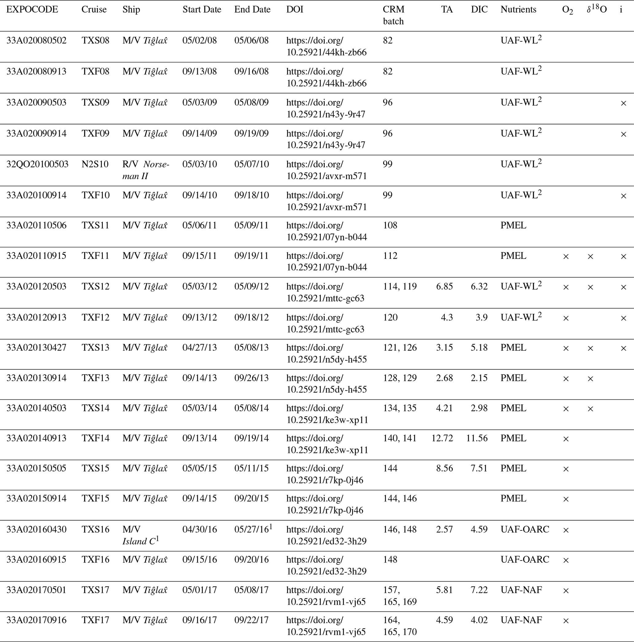
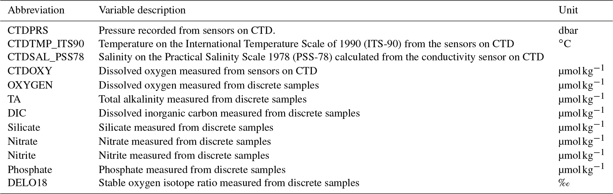
Table 2 Parameters included in this data product (adapted from Jiang et al., 2021).

When samples are collected at i stations, a half value is used. For example, at station GAK1i, the sample ID is 1.5, giving the sample collected at GAK1i, cast 3, Rosette position of 11 a Sample ID of 15311. Stations visited off the GAK Line, including repeat stations visited in most years within Prince William Sound (PWS, Fig. 1) and stations of opportunity, are not included in this data product. See Sect. 4 for additional information on stations and data collected outside the GAK Line.

Quality control (QC) steps on the cruise-level files follow previous studies (e.g., Jiang et al., 2021; Tanhua et al., 2010). First, the “zero step” QC is performed on individual measurements from instruments during collection. Next, the primary QC level used property–property plots to eliminate any outliers. Finally, we added an additional step to identify questionable data based on expected values using the regression according to Evans et al. (2013). Here we applied a multiple linear regression (MLR) based on an O₂-based algorithm to predict DIC. Then, we compared the derived DIC from our predictions to measured DIC to isolate measurements where the difference between measured and predicted values exceeded 4 times the root mean square error (RMSE) of the algorithm. The final QC step applied in this dataset is not comparable with the secondary level QC flags for global products such as the Global Ocean Data and Analysis Product (GLODAP, Lauvset et al., 2022). Both GLODAP and CODAP–NA use an additional QC process to identify biases in the data (Olsen et al., 2016, 2017). The data in this product have not been converted or corrected in any way for potential systematic biases.

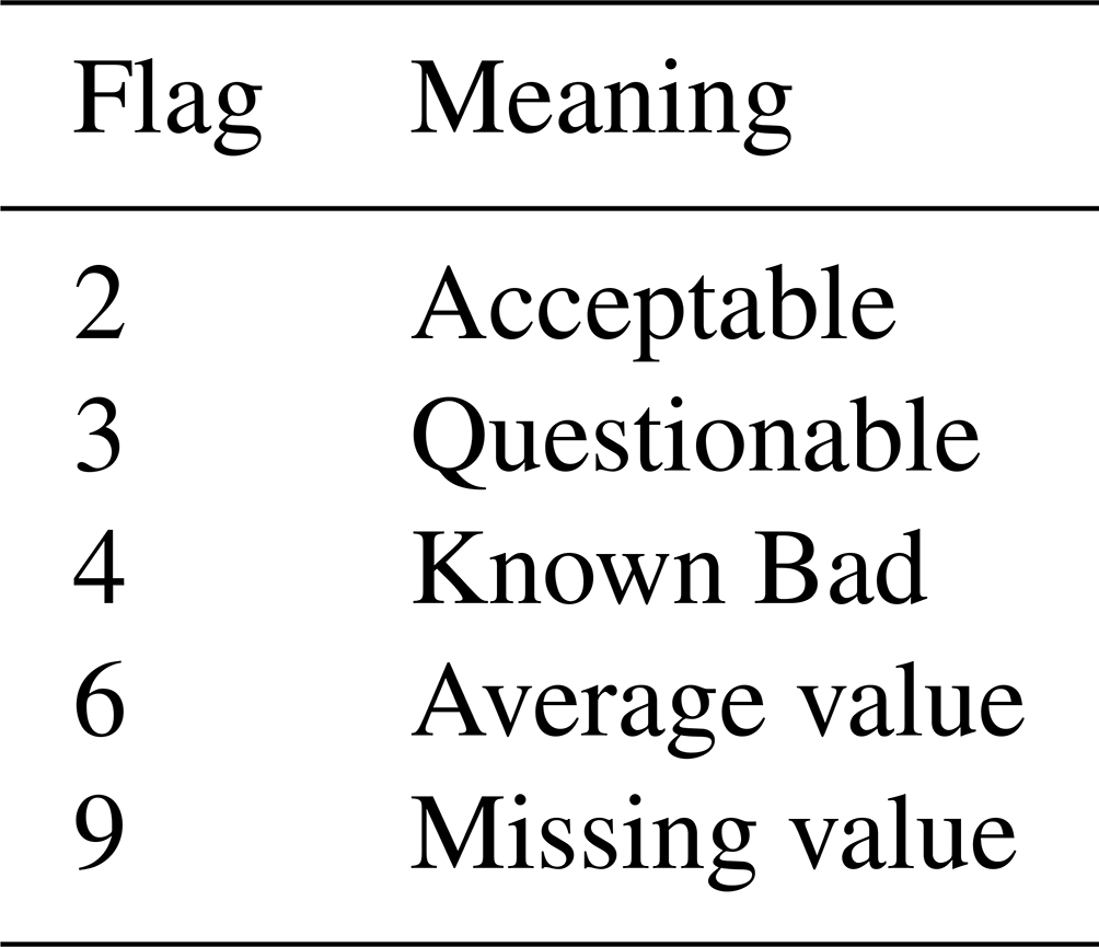
Quality flags (QFs) were applied to the cruise-level files according to best practices outlined in Jiang et al. (2022) and summarized in Table 3. This data product and corresponding figures in this publication only include GAK Line data when the measured carbonate parameters (TA and DIC) had a QF=2 (“acceptable”). No data identified as QF=3 (“questionable”) or QF=4 (“known bad”) are included in the merged data product. Owing to inconsistencies in nutrient sample collection and analysis methods in samples from cruises in 2008, 2009, 2010, and 2012, these data were assigned a QF=3 in the original cruise-level files and are also excluded from this data product (indicated by ² in the nutrients column in Table 1). This data product (Monacci et al., 2023) used “–999” and QF=9 (“not reported”) when the cruise-level data were assigned a QF other than 2. The individual cruise datasets include all data (Monacci et al., 2020a–j).

Table 3 Summary of standard primary-level quality control flags (Jiang et al., 2022) in this data product.

2.4 Calculations and Error

Using the analytical accuracy and precision of the Marine Analytics and Data (Marianda) built instruments, VINDTA and AIRICA, the uncertainty was calculated in quadrature using Eq. (2):

$$\begin{array}{}\text{(2)}& \text{Uncertainty}=\sqrt{{\text{accuracy}}^{\mathrm{2}}+{\text{precision}}^{\mathrm{2}}}.\end{array}$$

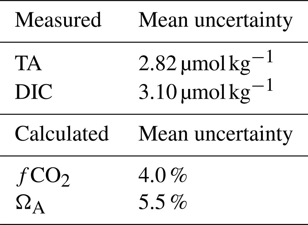
The mean handling error for TA and DIC are 5.54 ± 3.15 and 5.54 ± 2.74 µmol kg⁻¹ respectively, which is larger than the mean analytical uncertainty. Mean handling error, calculated from the triplicate discrete samples collected from the same Niskin bottle on most cruises (Table 1) are assumed to be representative of both sampling and storage uncertainties. Analytical precision and accuracy and the handling error we report here are averaged for all 20 cruise-level datasets. The mean analytical uncertainty for our measured variables, TA and DIC, are 2.82 and 3.10 µmol kg⁻¹ respectively (Table 4).

Table 4 Mean uncertainties of parameters calculated in CO2SYS. Input parameters are in situ T, S, and pressure and measured TA, DIC, phosphate, and silicate. Mean analytical uncertainties for the measured parameters DIC and TA are in quadrature, combining the accuracy and precision of the instruments.

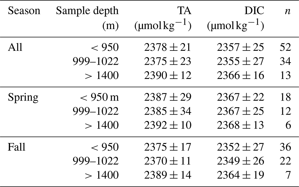
Owing to a low number of samples collected below a water depth of 1500 m, we were not able to perform a crossover analysis on deep-water property variability. Therefore, the most recently developed tool (Jiang et al., 2021) for inter-cruise comparisons and internal consistency was not used, and we do not have an inter-cruise error estimate as produced on other multi-cruise projects (e.g., Gouretski and Jancke, 2000; Johnson et al., 2001; Olsen et al., 2016). The internal consistency of the dataset is challenged in multiple ways, including the various methods used to sample and analyze nutrient measurements, as discussed above. However, it also routinely challenged the capacity of samplers to collect data relevant for inter-cruise comparisons. Deep-water sampling requires wire time not just for the CTD cast itself, but also weather windows and conditions that allow for sampling at the deepest station (GAK15). Accordingly, deep-water data in this dataset that could have been used for the calculation of internal consistency were only available in the early part of the dataset (before 2014). Furthermore, the low sample number (n; Table 5) of these samples also challenges the creation of a statistical mean against which a potential bias of each cruise could be measured. Accordingly, no bias in individual cruises was identified, and no correction for internal consistency was applied to any single mission in this dataset. Despite these high errors in deep-water sampling, note that there is sufficient surface water data to explore climatological changes with statistical significance elsewhere in this dataset.

Table 5 Deep water data used for the demonstration of internal consistency, including the average and standard deviation of DIC (µmol kg⁻¹) and TA (µmol kg⁻¹) data below 950 m, between 999 and 1022 m, and deeper than 1400 m across the entire dataset, in spring, and in fall. The number of samples used to derive these statistics is also shown.

We used a MATLAB version of CO2SYS (van Heuven et al., 2011) to calculate the fugacity of carbon dioxide (fCO₂), pH on Total Scale (pH_T), and saturation state for aragonite (Ω_A) when the measured input variables (T, S, DIC, TA, phosphate, and silicate) had a QF=2. In years where no nutrient data met the QF=2 criteria (e.g., 2008, 2009, 2010, 2012), we included a seasonal average nutrient value for that location and depth in the calculation. The nutrient alkalinity increases the fCO₂ and reduces the carbonate ion (${{\mathrm{CO}}_{\mathrm{3}}}^{\mathrm{2}-}$) value when the DIC–TA input pair is used (Orr et al., 2015); therefore, the averaged nutrient values are a better estimation than not including phosphate and silicate values. We applied the K₁ and K₂ stoichiometric constants from Millero et al. (2006), the $K_{{\mathrm{SO}}_{\mathrm{4}}}$ dissociation constant from Dickson (1990), and the K_B constant from Uppström (1974). New software packages have the capacity to compute propagated uncertainties (Dillon et al., 2020; Orr et al., 2018; Sharp and Byrne, 2021) for the calculated parameters. Using the Orr et al. (2018) application with average input values from this data product and the reference uncertainties results in percent relative combined standard uncertainty of nearly 4.0 % for fCO₂ and 5.5 % for Ω_A (Table 4).

2.5 Determining Controls on Surface fCO₂

We follow the approach by Wang et al. (2022), a modified method first developed by Takahashi et al. (2002), to calculate the interannual fCO₂ variability drivers, as well as the influence of sea surface temperature (T) and all other nonthermal processes (nT) on the fCO₂ anomaly using Eqs. (3) and (4):

$$\begin{array}{}\text{(3)}& {\displaystyle }T\left(\mathrm{\Delta }f{\mathrm{CO}}_{\mathrm{2}}\right)=f{\mathrm{CO}}_{\mathrm{2}}-nf{\mathrm{CO}}_{\mathrm{2}}.\text{(4)}& {\displaystyle }nT\left(\mathrm{\Delta }f{\mathrm{CO}}_{\mathrm{2}}\right)=nf{\mathrm{CO}}_{\mathrm{2}}-f{{\mathrm{CO}}_{\mathrm{2}}}_{\text{mean}}.\end{array}$$

Like Wang et al. (2022), the T and nT in this study are different from the thermal and nonthermal fCO₂ components calculated in Takahashi et al. (2002) owing to the unavailability of annual mean fCO₂ in high latitudes. Note that Eq. (4) is different from Wang et al. (2022) as we are calculating seasonal means of fCO₂, not ocean-atmosphere flux (F). Therefore, the quantity fCO_2 mean represents the climatological spring or fall means of fCO₂ and nfCO₂ is the temperature-normalized fCO₂ relative to the climatological mean spring or fall temperature using Eq. (5):

$$\begin{array}{}\text{(5)}& nf{\mathrm{CO}}_{\mathrm{2}}=f{\mathrm{CO}}_{\mathrm{2}}\times \exp \left(\mathrm{0.0423}\right(T_{\text{mean}}-T_{\text{obs}}\left)\right).\end{array}$$

Equation (5) is from Takahashi et al. (2002), where T_obs is the in situ temperature, and T_mean (Fig. 4) is the climatological spring or fall mean value. Wang et al. (2022) explains that Eq. (3) is a measure of the temperature effect, relative to the climatological seasonal mean temperature and Eq. (4) represents the impact of processes (e.g., biological CO₂ consumption or respiration, ocean-atmosphere CO₂ flux, and changes in carbonate ion concentrations) unrelated to temperature (e.g., Bates et al., 2013; Cross et al., 2013). Last, we calculate the fCO₂ anomaly using Eq. (6):

$$\begin{array}{}\text{(6)}& \begin{array}{rl}f{{\mathrm{CO}}_{\mathrm{2}}}_{\text{anomaly}}& =f{{\mathrm{CO}}_{\mathrm{2}}}_{\text{ocean}}-f{{\mathrm{CO}}_{\mathrm{2}}}_{\text{mean}}\\ & =T\left(\mathrm{\Delta }f{\mathrm{CO}}_{\mathrm{2}}\right)+nT\left(\mathrm{\Delta }f{\mathrm{CO}}_{\mathrm{2}}\right).\end{array}\end{array}$$

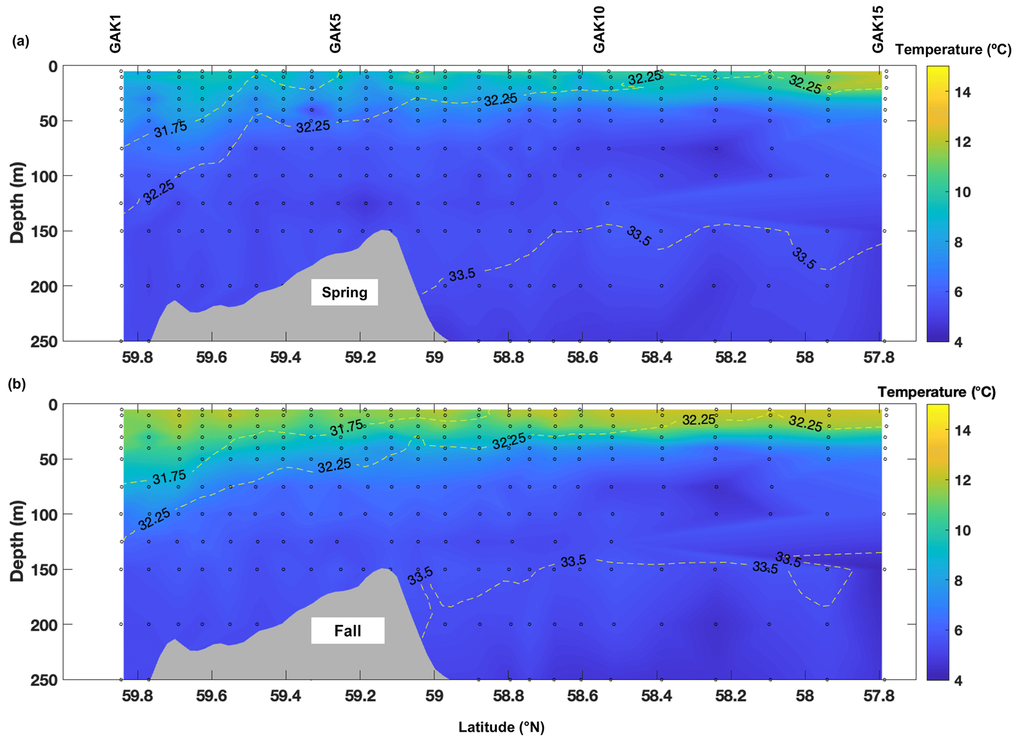
Figure 4 (a) The climatological average seawater temperature in the upper 250 m of the GAK Line transect in (a) spring (May) and (b) fall (September) during all the study years (2008–2017), plotted with salinity contours.

3 Dataset Demonstration

In this section, we offer some examples of the value and potential usage of this dataset for evaluating carbonate chemistry patterns and discuss how additional data collections may improve the quality, usability, and accessibility of the dataset. At present, we estimate that the value of this time series will be primarily for the exploration of climatological patterns in carbonate chemistry parameters. Below, we offer a climatological exploration of fCO₂ as an example. In general, we find that this dataset is of sufficient length and quality to determine some climatological trends in fCO₂, as well as to assess some of the potential physical drivers of this variability. However, physical parameters, such as temperature, do not sufficiently describe these emerging trends. Additional datasets and analysis are necessary to identify the mechanisms that underpin these changes. Overall, this dataset is good for exploring climatological mean states, some geochemical trends and variability, and the physicochemical contributions to this variability, but not for assessing potential biological contributions to carbon system variability.

3.1 Seasonality of fCO₂

The average spring (a) and fall (b) fCO₂ along the GAK Line are shown in Fig. 5. In general, seasonality was more evident in the intermediate depths (50–200 m), likely because of the known seasonal oscillation in downwelling strength. For example, 50 % of fall fCO₂ values fell within the 683–980 µatm range, which was slightly higher than the values from spring (600–967 µatm). By contrast, the average surface (upper 50 m) fCO₂ did not vary seasonally. The average surface fCO₂ in spring ranged from 247 to 450 µatm, with 50 % of data ranging from 309 to 363 µatm, lower than the atmospheric level. The average surface fCO₂ in fall was almost identical to spring, but with a few extreme outliers (460–528 µatm) because of episodic mixing events that brought higher fCO₂ from the deep layer to the surface layer. The median fCO₂ in the average surface layer in spring and fall were 329 and 336 µatm respectively. This average surface fCO₂ value is lower than atmospheric fCO₂, again indicating that this region is a year-round CO₂ sink, as previously documented (Evans and Mathis, 2013).

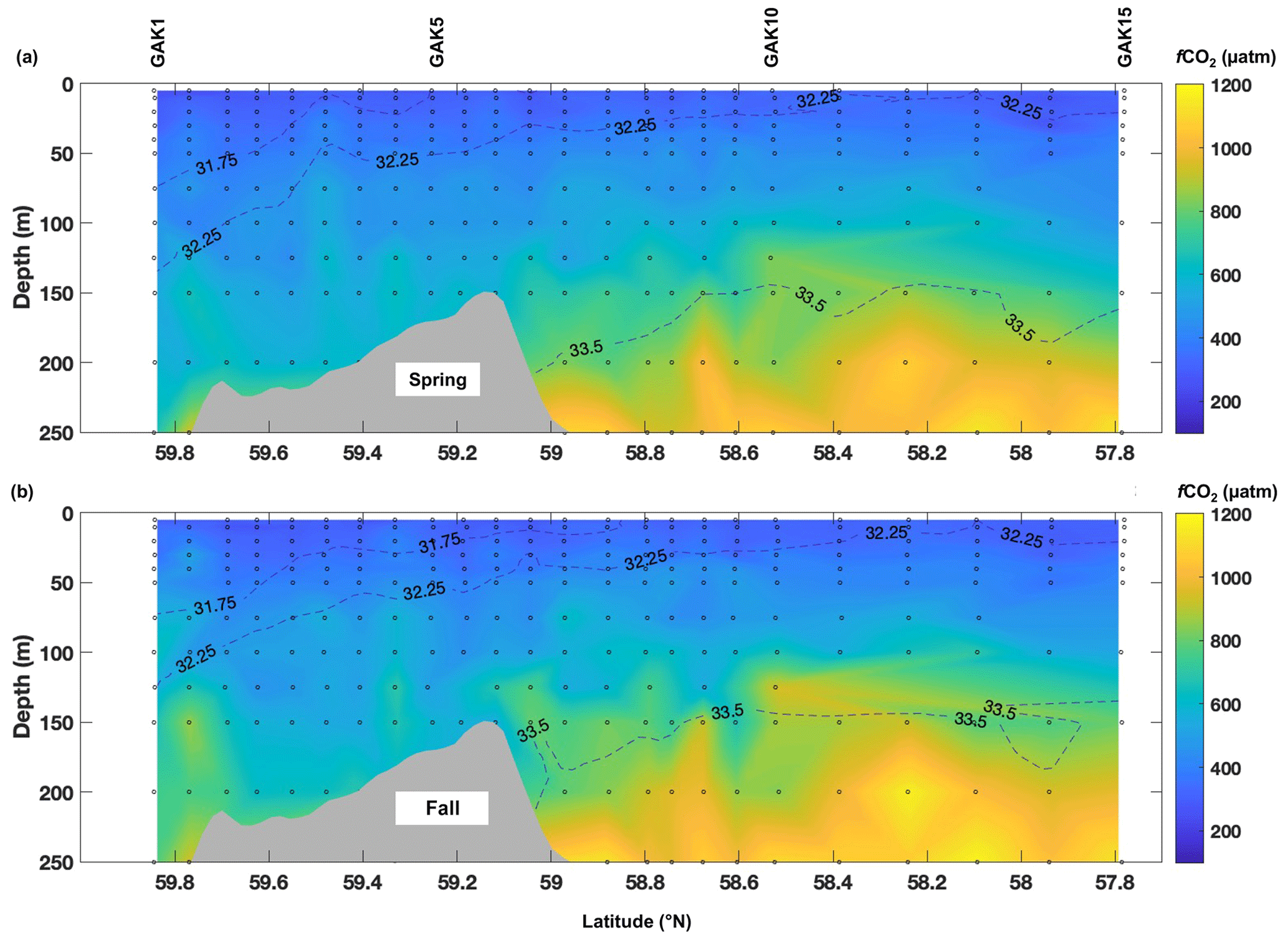
Figure 5 (a) The average fugacity of carbon dioxide (fCO₂) in the upper 250 m of the GAK Line transect in (a) spring (May) and (b) fall (September) during all the study years (2008–2017), plotted with salinity contours.

3.2 Climatology of Surface fCO₂

The climatological average fCO₂ in the surface (upper 50 m) was lower than the atmospheric fCO₂ value (Fig. 6), with episodic high fCO₂ events (>450 µatm) in both seasons. Interestingly, there were more episodic high fCO₂ values before 2014 in both seasons. Based on a temperature normalization analysis, temperature seems not to be the primary driver of either the long-term decline in average surface fCO₂ or the frequency and magnitude of the episodic high fCO₂ events. The T(ΔfCO₂) represents the impact of temperature anomalies on surface fCO₂. As temperature anomalies increase, fCO₂ and T(ΔfCO₂) increase first owing to a decrease in CO₂ dissolution. This is further compounded by shifts in equilibrium that favor reactants, specifically, CO₂ and H₂O, over their product forms (H₂CO₃, ${{\mathrm{HCO}}_{\mathrm{3}}}^{-}$, and ${{\mathrm{CO}}_{\mathrm{3}}}^{\mathrm{2}-}$). Consequently, more CO₂ remains in its initial, unreacted state. However, there were no clear temporal changes from T(ΔfCO₂) between before 2014 and after 2014, anomalies were less than 50 µatm, which cannot explain the >200 µatm episodic changes. Therefore, our analyses suggest that other nonthermal processes, such as anomalies in productivity/respiration, may well lead to interannual variations in surface fCO₂. Anomalies in the patterns of primary productivity and respiration may, at least to a first order, be related to patterns in regional wind forcing, and we note that 2011–2013 displayed some of the weakest CDUI values over the start of each year in this dataset (Fig. 2). Weaker CDUI values over the first half of the year would imply reduced winter downwelling and storm activity, which acts to replenish surface nutrients. A reduction in stormy conditions would precondition the system for weaker spring phytoplankton blooms, either by weaker nutrient replenishment or a change in the phenology of the spring phytoplankton bloom to groups that favor more stratified conditions. Such a state could lead to a weaker and shallower extent of undersaturated surface water with respect to the atmosphere, which may then be easily mixed by episodic wind forcing and lead to the observed fCO₂ anomalies. The relationship between the magnitude and frequency of these high fCO₂ events, the relaxation of downwelling, and influences on primary productivity requires additional investigation.

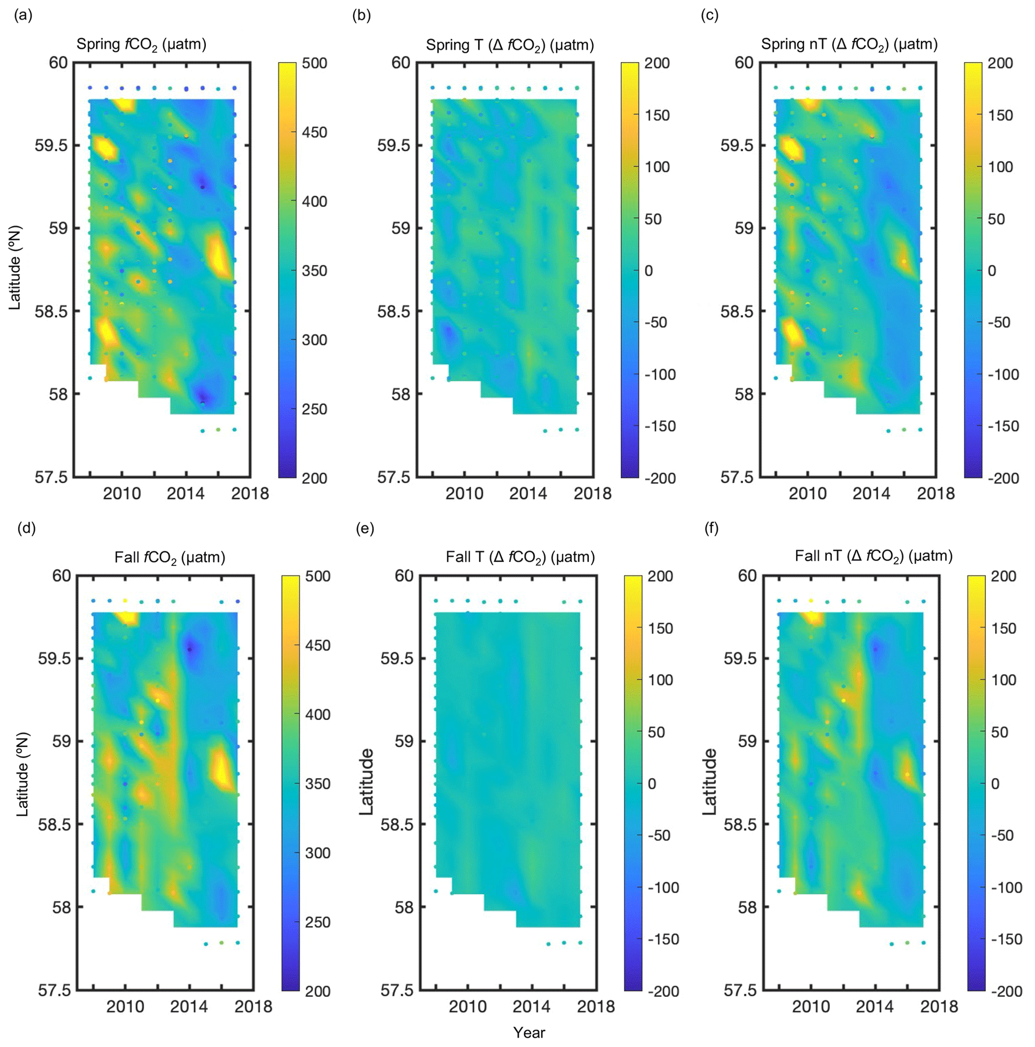
Figure 6 The fugacity of carbon dioxide (fCO₂) is impacted by sea surface temperature (T, Eq. 3) and other nonthermal processes (nT, Eq. 4). Panels show the upper 50 m of the water column average along the GAK Line transect from 2008 to 2017 for the (a) spring fCO₂, (b) thermally driven spring fCO₂ anomaly [T(ΔfCO₂)], (c) nonthermal spring fCO₂ anomaly [nT(ΔfCO₂)], (d) fall fCO₂, (e) fall T(ΔfCO₂), and (f) fall nT(ΔfCO₂).

3.3 Spatiotemporal trends of CO₂

In addition to showing the climatological average spring and fall modes of fCO₂ variability, the time–series component of this dataset can also be used to understand the CO₂ sink changes over time. In Fig. 7, we split the data into three regional components to show emerging trends in the upper 50 m of different sub-regions of the Seward Line (Fig. 1): nearshore (GAK1–2), middle (GAK3–7), and offshore (GAK8–15). If the surface CO₂ increases have been slower than in the atmosphere, this region has been a decreasing CO₂ sink during the period studied. Sutton et al. (2019) reported the time of emergence (TOE) of anthropogenic CO₂ change depends on the internal variability, which was generally >20 years in coastal regions. Therefore, we acknowledge that the temporal span of these observations is from 2008 to 2017, which may not be sufficient to represent the long-term anthropogenic trends. Indeed, the CO₂ trend was insignificant in the nearshore regions in both spring and fall because of the high interannual variability (Fig. 7). Although the anthropogenic CO₂ trend did not emerge from the short record in fall or nearshore subregions, we did find significant variability in the middle and offshore subregions: the surface CO₂ has been significantly decreased in the spring. As discussed in Fig. 6b, the influence of temperature anomalies on the fCO₂ anomaly is minor compared with nT(ΔfCO₂); thus, the consistent T cannot explain the decreasing fCO₂ trend: enhanced primary productivity should support the lower surface fCO₂ (∼250 µatm) in nearshore and offshore regions after 2014. The increasing primary productivity made this area a rising carbon sink in spring after 2014. However, there is not sufficient information in this dataset to confirm this hypothesis. Sampling in May and September does not sufficiently bracket the spring bloom and is too long for the reliable calculation of seasonal net community production from DIC or nutrient measurements based on best practices (e.g., Mathis et al., 2009). Combining the data shown here with moored datasets, such as from GAKOA (Monacci et al., 2022), and remotely sensed biological parameters, such as chlorophyll, may be a fruitful line of future enquiry.

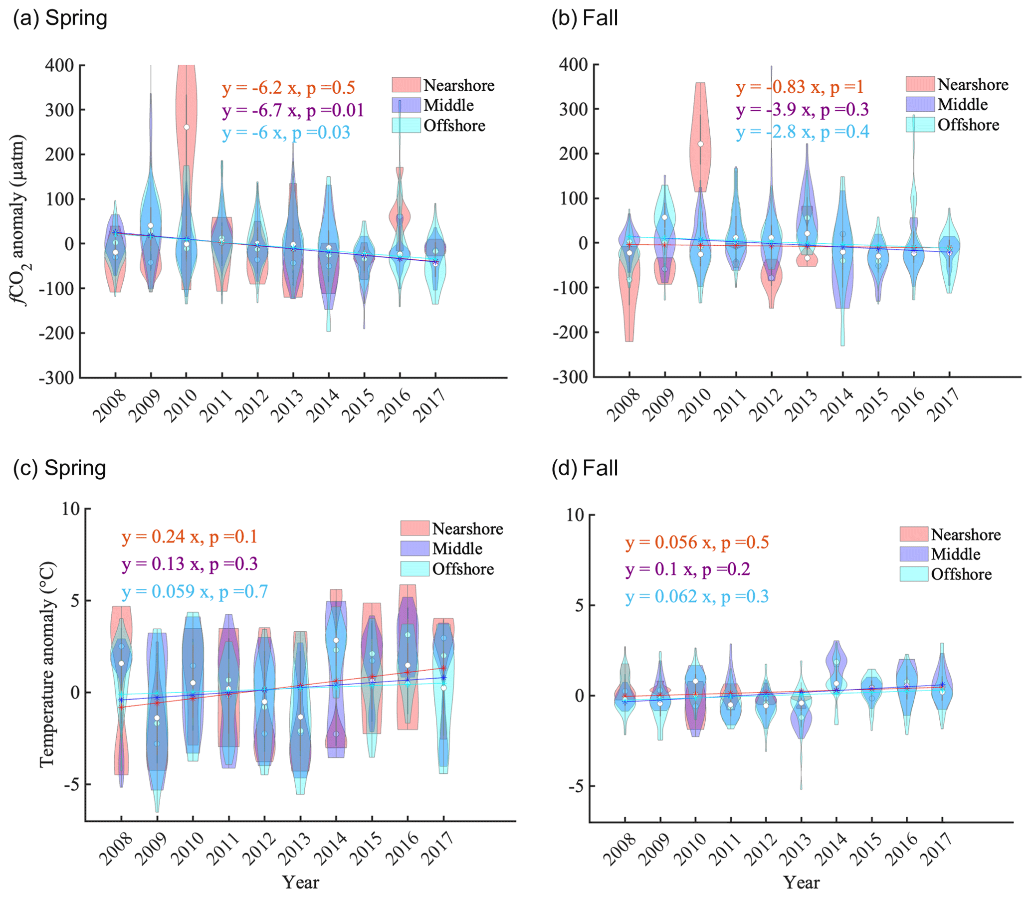
Figure 7 Regional (nearshore, middle, offshore) violin plots of the upper 50 m fCO₂ and temperature anomaly for spring (a, c) and fall (b, d). Seward Line stations (Fig. 1) are defined in regions: nearshore (GAK1–2), middle (GAK3–7), and offshore (GAK8–15).

4 Data availability

The digital object identifier (DOI) for this merged data product is https://doi.org/10.25921/x9sg-9b08 (Monacci et al., 2023). Users looking to access marine carbonate parameter data for the GAK Line that have been designated as good (QF=2) should consider using this data product. The cruise-level DOIs listed in Table 1 are archived at the National Oceanic and Atmospheric Administration (NOAA) National Centers for Environmental Information (NCEI) (Monacci et al., 2020a–j). These data can also be accessed from the NOAA NCEI Ocean Carbon and Acidification Data System (OCADS) project page: Seward Line Cruises 2008–2017 https://www.ncei.noaa.gov/access/ocean-carbon-acidification-data-system/oceans/Coastal/seward.html (last access: 2 August 2023). Users interested in all available data should use the cruise-level data at NCEI (Table 1). Users should also be aware that the GAK Line was visited during the NOAA Ship Ronald H. Brown cruise RB1504 (EXPOCODE 33RO20150713) in July 2015. The RB1504 cruise was funded by the NOAA Ocean Acidification Program and data are archived under the DOI https://doi.org/10.25921/dey6-9h45 (Cross et al., 2019).

Data collected during 2008–2012 have been used by Shake (2011) to describe seasonal variability, Evans and Mathis (2013) to determine the Gulf of Alaska as a CO₂ sink, Evans et al. (2013) to develop a regression modeling approach to understand variability, and Hauri et al. (2020) and Siedlecki et al. (2017) to validate regional models. The cruise-level data sets (Table 1) include observations from the western PWS (Fig. 1) but are not included in this merged data product for the GAK Line. Carbonate system data collected in PWS on May and September cruises from 2009 to 2012 were reported in Evans et al. (2014) and Cai et al. (2021). The datasets were not publicly archived at the time of these publications and future uses and references should include the appropriate dataset citations (Monacci et al., 2020a–j). There continues to be a shortage of dataset citations in publications (Vannan et al., 2020), and this data product is direct proof of our support to make data accessible, usable, and citable. We ask users to invite collaboration with the scientific investigators on these datasets as they can provide additional insight. Citation and collaboration are not only good practice but also promote sharing of data and advancing of accessibility.

5 Conclusion

This data product provides a distinct data set for users interested in the NGA ecosystem, coastal carbon dynamics, ocean acidification, biogeochemical cycling, and ocean change. It can be used to explore natural environmental variability in the physical system and its impacts on marine carbonate parameters. Our examples provide assessments of seasonal, interannual, and regional differences. The timespan of this data product is too short to explore the rate of anthropogenic CO₂ absorption, although there are sustained observations in the region using a moored autonomous pCO₂ (MAPCO2™, Sutton et al., 2019) system and through the National Science Foundation's program NGA–LTER. Ocean time series allow us to understand long-term change and can be an important tool in developing predictions and solutions to continued anthropogenic perturbations. As the global economy turns to the ocean for additional CO₂ sequestration in marine carbon dioxide removal (mCDR) methods, our reliance on time series sites for our calculations is likely to expand. This data product fills a large gap in the publicly accessible inorganic carbon measurements for a subarctic environment. Although our efforts have fallen short of some best practices (e.g., discrete salinity and nutrient measurements) outlined in GLODAPv2 (Olsen et al., 2016), we feel that our carbonate parameter measurements are consistent with the OA community goals and standards.