High-resolution (1 km) all-sky net radiation over Europe enabled by the merging of land surface temperature retrievals from geostationary and polar-orbiting satellites

Surface net radiation (SNR) is a vital input for many land surface and hydrological models. However, most of the current remote sensing datasets of SNR come mostly at coarse resolutions or have large gaps due to cloud cover that hinder their use as input in models. Here, we present a downscaled and continuous daily SNR product across Europe for 2018–2019. Long-wave outgoing radiation is computed from a merged land surface temperature (LST) product in combination with Meteosat Second Generation emissivity data. The merged LST product is based on all-sky LST retrievals from the Spinning Enhanced Visible and InfraRed Imager (SEVIRI) onboard the geostationary Meteosat Second Generation (MSG) satellite and clear-sky LST retrievals from the Sea and Land Surface Temperature Radiometer (SLSTR) onboard the polar-orbiting Sentinel-3A satellite. This approach makes use of the medium spatial (approx. 5–7 km) but high temporal (30 min) resolution, gap-free data from MSG along with the low temporal (2–3 d) but high spatial (1 km) resolution of the Sentinel-3 LST retrievals. The resulting 1 km and daily LST dataset is based on an hourly merging of both datasets through bias correction and Kalman filter assimilation. Short-wave outgoing radiation is computed from the incoming short-wave radiation from MSG and the downscaled albedo using 1 km PROBA-V data. MSG incoming short-wave and long-wave radiation and the outgoing radiation components at 1 km spatial resolution are used together to compute the final daily SNR dataset in a consistent manner. Validation results indicate an improvement of the mean squared error by ca. 7 % with an increase in spatial detail compared to the original MSG product. The resulting pan-European SNR dataset, as well as the merged LST product, can be used for hydrological modelling and as input to models dedicated to estimating evaporation and surface turbulent heat fluxes and will be regularly updated in the future. The datasets can be downloaded from https://doi.org/10.5281/zenodo.8332222 (Rains, 2023a) and https://doi.org/10.5281/zenodo.8332128 (Rains, 2023b).

1 Introduction

The Earth radiation budget describes how the Earth gains energy from the Sun (short-wave radiation) and loses energy back to space through its reflection and the emission of thermal (long-wave) radiation (Dewitte and Clerbaux, 2017; Kato et al., 2018). Due to the geometry of the Earth's orbit around the Sun, the yearly average net radiation at the bottom of the atmosphere, namely the surface net radiation (SNR), is positive at the Equator and decreases towards the poles. This geographical energy imbalance is the main driver of the global atmospheric and oceanic circulation, which transports this energy surplus from the Equator towards the poles (Dewitte and Clerbaux, 2017; Kato et al., 2018). SNR is thus a key driver in explaining the distribution of different climate regions and ecosystems on Earth (Köppen and Geiger, 1936), and it dominates the dynamics of biospheric and hydrological processes (Chapin et al., 2002). For this reason, SNR is used as forcing variable in many land surface models, hydrological models and satellite-based retrieval algorithms to estimate (e.g.) evaporation, runoff, soil moisture or surface heat fluxes.

The top-of-atmosphere radiation components can be derived directly from satellites. However, dynamic atmospheric (e.g. cloud and aerosol optical depth) and land (e.g. emissivity, land surface temperature (LST), albedo or biomass) properties make it more challenging to obtain radiation estimates at the bottom of the atmosphere, which are much more relevant to the above-mentioned biospheric and hydrological processes. As it is transmitted through the atmosphere, incoming short-wave radiation is scattered and absorbed by aerosols, gases and clouds, changing the temperature of the atmosphere and its emission of long-wave radiation in all directions. The radiation reaching the surface is partly reflected, depending on the land cover and surface conditions, and again interacts with the atmosphere/clouds once reflected. According to Stephens et al. (2012), on average, 12 % of the radiation reaching the surface is reflected back into the atmosphere; this is known as the surface planetary albedo. Then, part of the incoming radiation absorbed at the land surface is emitted towards the atmosphere as long-wave radiation, as described by the Stefan–Boltzmann law. The modelling of these atmospheric and surface processes is required to obtain the SNR – i.e. the balance between short-wave and long-wave incoming and outgoing radiation at the surface – and it makes satellite-based SNR retrievals indirect and uncertain (Kato et al., 2018).

Over the past decades, numerous satellites/instruments have been launched to enable the monitoring of the radiation budget. Examples of programmes exploiting these observations to produce long-term global reliable estimates of the individual SNR components (i.e. short-wave and long-wave, and both incoming and outgoing) are the International Satellite Cloud Climatology Project (ISCCP, Young et al., 2018) and the Clouds and the Earth's Radiant Energy System (CERES) project (Wielicki et al., 1996). A comparison between the CERES product and radiation estimates from global reanalyses is given by Jia et al. (2018). Both satellite-based and reanalysis SNR products are mostly provided at a coarse (ca. 0.25^∘) spatial resolution. This makes them suitable for global analysis or as input in global land surface models but insufficient for most regional-scale studies. A few studies have already attempted to produce SNR data at higher spatial resolutions. For instance, Verma et al. (2016) proposed a method to yield a global 5 km SNR product at 8 d resolution by combining high-resolution variables derived from the Moderate Resolution Imaging Spectroradiometer (MODIS) Aqua satellite (including clear-sky LST, emissivity, aerosol optical depth and albedo) and a radiative transfer model with ancillary datasets from reanalysis. Also with a resolution of 5 km, Jiang et al. (2016, 2018) developed the Global Land Surface Satellite (GLASS) daily daytime net radiation product based on multivariate adaptive regression splines, combining incoming short-wave radiation, albedo and normalized difference vegetation index (NDVI) with further meteorological ancillary variables, such as wind speed, surface pressure and air temperature. Meanwhile, Jiang et al. (2023) developed a methodology, based on Landsat data and ancillary datasets, that uses machine learning to produce the daily net radiation at 30 m resolution. As an alternative to such methods (which are based on data from polar-orbiting satellites), to achieve a much higher temporal resolution (sub-daily) at the expense of spatial resolution, observations from geostationary satellites can be used. The Satellite Applications Facility (LSAF) programme uses observations from the SEVIRI instrument onboard the Meteosat Second Generation (MSG) satellite to produce a SNR dataset at a spatial resolution of ca. 5–7 km (Trigo et al., 2011). These resolutions, however, still appear to be insufficient for regional water and agricultural management assessments in heterogeneous landscapes.

In this study, we present a 1 km SNR, and LST, dataset for Europe using MSG and polar orbiting observations. It is based on combining operationally available hourly incoming short-wave/long-wave radiation retrievals from the above-mentioned LSAF programme at moderate (5–7 km) spatial resolution with hourly LSAF LST estimates as well as higher resolution (1 km) albedo retrievals from PROBA-V and LST from Sentinel-3 (Donlon et al., 2012). The novelty of this study lies in systematically exploiting the advantages, and mitigating the disadvantages, in terms of the spatial and temporal resolution of available observations, which are well validated, in a physical and consistent manner based on the surface energy balance, and assembling a net radiation dataset from the individual incoming and outgoing radiation components. This includes the development of a 1 km gap-free LST product for downscaling outgoing long-wave radiation. All-sky estimates are particularly important for LST, as cloud cover severely restricts the availability of clear-sky retrievals and it is temporally highly variable. This is underpinned by a number of previous studies which have focused on producing all-sky LST estimates; see e.g. Xu and Cheng (2021) and Jia et al. (2023), the latter also exploiting observations from geostationary and polar-orbiting products. 1 km albedo, used for the computation of outgoing short-wave radiation, is also calculated by combining polar and geostationary observations. The merged hourly SNR and LST data are resampled to daily time steps for robustness. The coarse-scale (5–7 km) all-sky LST estimates provided through the LSAF programme have only recently been released, and the methodology used here aims at exploiting these new data in an optimal manner. To our understanding, a systematic combination of these polar and geostationary retrievals with the overall goal of calculating a consistent high-resolution SNR product has not yet been undertaken. We argue that this approach based on the surface energy balance is the most consistent and, in theory, should yield the most accurate results.

The published data presented here is especially meant for use as a high-resolution forcing dataset for models which require the SNR, such as The Global Land Evaporation Amsterdam Model (GLEAM). Such models can also benefit from high-resolution all-sky LST data, making the intermediate merged LST product equally useful. In principle, the methodology can be extended to regions where the same variables are available from other geostationary and polar-orbiting satellites. The data and method are presented in detail in Sects. 2 and 3. All input and derived radiation components are validated against in situ measurements from sites located across the study domain (Sect. 4) and the SNR dataset is compared to ERA5-Land (Muñoz-Sabater et al., 2021). Finally, a discussion with respect to similar studies and concluding remarks are given in Sects. 5 and 7. The daily SNR and LST datasets are available for scientific use under https://doi.org/10.5281/zenodo.8332222/ https://doi.org/10.5281/zenodo.8332128 as netcdf files (RNETdaily_lon_lat.nc and LSTdaily_lon_lat.nc); see Rains (2023a) and Rains (2023b). The spatial domain covered is −11.5 to 26.5^∘ longitude and 35 to 71^∘ latitude. The initial dataset is available for the years 2018–2019.

2 Data

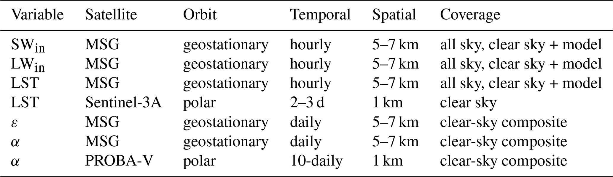
Table 1 provides a general overview of the satellite data products used in this study. Short-wave and long-wave incoming radiation components, SW_in and LW_in respectively, as well as the emissivity ε, albedo α and LST are provided by LSAF (lsa-saf.eumetsat.int) and are based on observations from the Spinning Enhanced Visible and InfraRed Imager (SEVIRI) instrument onboard the Meteosat Second Generation (MSG) geostationary satellite. These MSG products are provided with 30 min sampling, but to reduce data volumes we base our methodology on hourly data. The spatial resolution across the European domain is approximately 5–7 km depending on the latitude. In addition, 1 km LST retrievals from the Sea and Land Surface Temperature Radiometer (SLSTR) instrument onboard Sentinel-3 as well as 1 km albedo retrievals from PROBA-V are used to compute the high-resolution LST dataset and outgoing radiation components. For the purpose of validation, we use radiation measurements from sites distributed across Europe belonging to different international networks. A more detailed description of the satellite retrievals and in situ data used in the study is provided in the following subsections. Note as well that ERA5-Land (Muñoz-Sabater et al., 2021) is also used in Sect. 4 for comparison purposes.

Table 1 Overview of satellite-based products used in the study, with their respective temporal and spatial resolutions as well as their coverage, i.e. clear sky vs all sky.

2.1 Incoming short-wave/long-wave radiation

We use hourly data from the LSAF programme, part of the distributed Applications Ground Segment SAF network serving as the European Organisation for the Exploitation of Meteorological Satellites (EUMETSAT). The data are based on observations provided by SEVIRI onboard MSG and acquired at 12 spectral channels with 3 km resolution at nadir (1 km for the high-resolution visible channel) (Trigo et al., 2011). A detailed description of the LSAF methodology for deriving SW_in and its validation is given by Carrer et al. (2019a) and Carrer et al. (2019b). Details on the estimation and evaluation of LW_in are given by Trigo et al. (2010) and Carrer et al. (2012).

2.2 LST

The LSAF all-sky LST product based on the SEVIRI instrument onboard the geostationary Meteosat Second Generation (MSG, Martins et al., 2019) is a combination of the clear-sky MSG level 2 product MSLT (LSA-001), based on a generalised split-window (GSW) algorithm (Trigo et al., 2008a), and output from an energy balance algorithm which is also used for the production of the MSG 30 min evaporation (MET-v2, LSA-311) dataset (Ghilain, 2016). The energy balance algorithm incorporates other LSAF SEVIRI-based products such as short-wave and long-wave radiation fluxes, land surface albedo or vegetation, soil moisture based on the assimilation of scatterometer observations provided by the Hydrology SAF (H-SAF), and near-surface meteorological information obtained from the European Centre for Medium-Range Weather Forecasts (ECMWF) operational forecasts (Ghilain et al., 2020). Within the model, each pixel is composed of different tiles representing a particular surface type based on the ECOCLIMAP-II database (Faroux et al., 2013). Pixel values are computed from the weighted average of the four most dominant tiles. The advantage of using geostationary satellites is the high temporal resolution, which allows for the characterisation of the LST diurnal cycle. An assessment of the accuracy of the LST is given by Martins et al. (2019). The product comes with gridded uncertainty estimates, which are used in the LST merging procedure. Higher-resolution, clear-sky LST estimates are obtained from Sentinel-3. The Sentinel-3 mission consists of two polar-orbiting satellites (Sentinel-3A/B) launched on 16 February 2016 and 25 April 2018 (Ghent et al., 2017; Zheng et al., 2019; Nie et al., 2021), both carrying the Sea and Land Surface Temperature Radiometer (SLSTR) instrument. They have a revisit time of 2–3 d. The instrument has nine channels, three of them covering the visible and near-infrared (VNIR) part of the spectrum, three the short-wave infrared (SWIR) part, and the remaining three the middle-infrared (MIR and TIR, Nie et al., 2021) part. For this study, we use the Climate Change Initiative (CCI) LST product provided at a spatial resolution of 0.01^∘ (https://climate.esa.int/en/odp/#/project/land-surface-temperature, last access: 1 August 2022). Included in the product is the exact overpass time and, as for the LSAF LST from MSG, the total estimated uncertainty for each retrieval, necessary for the merging of the polar and geostationary LST data. For this initial study focusing on 2018–2019, only Sentinel-3A data were used. Sentinel-3B was launched in April 2018 and flown in tandem with Sentinel-3A from June to October of the same year, after which it was moved to its nominal orbit (Clerc et al., 2020). The approximate local overpass time of Sentinel-3A and Sentinel-3B thereafter is the same (ca. 10:30 am/pm), with the precise time varying and taken into account in the merging methodology (see Sect. 3.3).

2.3 Surface emissivity

The land surface ε is required, in conjunction with LST, to calculate LW_out. Methods to retrieve ε can be broadly separated into those where LST and ε are jointly retrieved and those where ε is retrieved in isolation. The latter approach was initially used within the LSAF programme and relied on spectral data for the various land covers (based on spectral libraries) and dynamic land cover fractions (Peres and DaCamara, 2005). To overcome difficulties linked to performing the retrieval of LST and ε separately under certain conditions, e.g. in semiarid regions, LST and ε are now simultaneously retrieved by the LSAF programme, including for the products we use in this study (Trigo et al., 2008b).

2.4 Albedo

The LSAF α product based on the MSG SEVIRI instrument is produced in three steps: (1) an atmospheric correction of top-of-atmosphere measurements to obtain reflectances, (2) a daily inversion of a semi-empirical model of the bidirectional reflectance distribution function and then the consideration of all inversions within a temporal window to reduce the impact of outliers and reduce data gaps, and (3) the angular integration for each channel and the spectral integration (Geiger et al., 2008; Carrer et al., 2018). The product thus describes the hemispherical broadband α. As a second hemispherical broadband α product, we use 1 km retrievals based on ProbaV and distributed through the Copernicus Global Land Service (CGLS). The retrieval follows the same methodology as for the LSAF α product.

2.5 In situ measurements

For the validation of the merged daily SNR dataset and the individual radiation components, we use radiation measurements taken at a total of 73 sites distributed across Europe for the 2-year study period (2018–2019). Measurements are obtained from the Baseline Surface Radiation Network (BSRN) (Driemel et al., 2018), the European Fluxes Database Cluster (EFDC; http://www.europe-fluxdata.eu, last access: 1 August 2022), the Integrated Carbon Observation System (ICOS) (Heiskanen et al., 2021), the FLUXNET-CH4 network (Delwiche et al., 2021), and SAPFLUX (Poyatos et al., 2021). Table , see Appendix A, provides a comprehensive list of the in situ sites used for this study. For a number of sites, all radiation components are available (54), while for others only a subset is available. The table includes the station ID, name, geographic coordinates and the international geosphere-biosphere programme (IGBP) land cover class as well as which radiation components are available for validation. The following land cover classes are covered: cropland (CRO), closed shrublands (CSH), deciduous broadleaf forest (DBF), evergreen needleleaf forest (ENF), grassland (GRA), mixed forest (MF), open shrublands (OSH), savanna (SAV), urban (URB), wetland (WET) and woody savanna (WSA). While the in situ measurements are considered as ground truth, it is necessary to mention that they have their own sources of uncertainties. Incoming short-wave and long-wave radiation are measured by pyranometers and pyrgeometers. Accuracy targets for the BSRN network measurements (from 2004) are, for example, 2 % or 5 W m⁻² for incoming short-wave radiation and 2 % or 3 W m⁻² for incoming long-wave radiation. Target uncertainties for outgoing short-wave and long-wave radiation are 3 % and 2 % (or 3 W m⁻²) respectively (McArthur, 2004). For the measurement of the outgoing radiation components, the pyranometer/pyrgeometer is installed facing downwards. The target uncertainties are in line with the achievable accuracy of the pyranometer/pyrgeometer instruments, although they might not be met under some conditions, e.g. incorrect installation at an angle or snow cover. The instruments should be calibrated, e.g. every 2 years (Walter-Shea et al., 2019).

3 Methodology

3.1 SNR calculation

SNR is computed using the radiation balance equation (1):

$$\begin{array}{}\text{(1)}& \mathrm{SNR}=({\mathrm{SW}}_{\mathrm{in}}+{\mathrm{LW}}_{\mathrm{in}})-({\mathrm{SW}}_{\mathrm{out}}+{\mathrm{LW}}_{\mathrm{out}}),\end{array}$$

where SW_in is the hourly incoming short-wave radiation (W m⁻²) and LW_in is the hourly incoming long-wave radiation (W m⁻²), both from LSAF (see Sect. 2). SW_out and LW_out are the hourly outgoing short-wave and outgoing long-wave radiation (W m⁻²), respectively, calculated as

$$\begin{array}{}\text{(2)}& {\displaystyle }{\mathrm{SW}}_{\mathrm{out}}={\mathrm{SW}}_{\mathrm{in}}\cdot \mathit{\alpha }\text{(3)}& {\displaystyle }{\mathrm{LW}}_{\mathrm{out}}=\mathit{\epsilon }\cdot \mathit{\sigma }\cdot {\mathrm{LST}}^{\mathrm{4}}+(\mathrm{1}-\mathit{\epsilon })\cdot {\mathrm{LW}}_{\mathrm{in}},\end{array}$$

with σ being the Stefan–Boltzmann constant (i.e. $\mathrm{5.67}\times {\mathrm{10}}^{-\mathrm{8}}$ W m⁻² K⁻⁴). Both SW_out and LW_out are to a large degree controlled by land surface properties and processes, i.e. SW_out by α (Eq. 2) and LW_out by ε and the LST (Eq. 3). The LST, in particular, dictates the magnitude and variability of LW_out over different spatial and temporal scales. Note that the term $(\mathrm{1}-\mathit{\epsilon })\cdot {\mathrm{LW}}_{\mathrm{in}}$ accounts for long-wave reflection (Maes and Steppe, 2012).

The focus here is on the improvement of the spatial resolution of the LSAF SW_out and LW_out by using the gap-free all-sky 1 km α and the LST in Eqs. (2) and (3), respectively. The details of these datasets are given in Sect. 3.2 and 3.3. The rationale is based on the assumption that SW_out and LW_out, especially on the daily scale which we aggregate to, are spatially more heterogeneous than the incoming components. Therefore, by using higher-resolution α and LST, the final SNR dataset can better capture the variability induced by landscape features and conditions.

3.2 Bias correction of albedo

To obtain a spatially and temporally gap-free α dataset at 1 km resolution, we bias correct the daily α from LSAF towards the retrievals from ProbaV using the mean of the temporally overlapping retrievals for 2018–2019. Remaining gaps are filled by linearly interpolating/extrapolating based on the nearest data points in the temporal domain. Prior to the bias correction, the α products are regridded using nearest-neighbour interpolation to a common 0.01^∘ grid. Since both sets of α are based on the same methodology, we assume that the bias can be largely attributed to the difference in spatial resolution, but also to the MSG product integrating multiple observations per day and possibly to the differences in the channels (ProbaV and SEVIRI response functions).

3.3 Merging of LST

The merging of the hourly LSAF LST (5–7 km) and Sentinel-3 LST (1 km) relies on the assumption that the diurnal cycle of LSAF is reliable in relative terms, whereas the Sentinel-3 LST can be trusted in absolute terms. This approach allows us to benefit from the high temporal resolution of the geostationary data and the high spatial resolution of the Sentinel-3 observations. The all-sky LSAF product, which contains a modelled LST when cloud cover prevents direct retrieval, enables the merged gap-free LST product with Sentinel-3 resolution. After regridding the LSAF observations, using nearest-neighbour interpolation, to the 0.01^∘ grid of Sentinel-3 observations, we follow a stepwise approach:

1. Temporal normalisation of Sentinel-3 daytime/nighttime observations on the hour.
   The Sentinel-3 LST is available every ∼ 2–3 d both during daytime (∼ 10:00 am local time) and during nighttime (∼ 10:00 pm local time), conditioned on the presence of clear skies. However, because of slightly differing overpass times from day to day, we first normalise the Sentinel-3 daytime/nighttime observations individually to be on the hour (e.g. at 10:00 for daytime) using information from the diurnal cycle described by the hourly LSAF observations of the same day. For that, at each grid cell, we convert the on-the-hour daytime and nighttime overpass time of the Sentinel-3 observations from local time to UTC. Then, when a Sentinel-3 daytime or nighttime observation is acquired, e.g. prior to that mean UTC daytime or nighttime overpass hour t, the observation is corrected through linear interpolation using the LSAF LST retrievals at t and the previous hour t−1 on that day:

   $$\begin{array}{ll}{\displaystyle }{\text{Sentinel 3LST}}_{\mathrm{nor}}& {\displaystyle }=\text{Sentinel 3LST}+\mathrm{\Delta }t\\ {\displaystyle }& {\displaystyle }\cdot ({\mathrm{LSAFLST}}_t-{\mathrm{LSAFLST}}_{t-\mathrm{1}}),\end{array}$$

   with Δt being the difference between the on-the-hour mean nighttime/daytime overpass time t and the exact overpass time of the specific Sentinel-3 observation on that day. We do not perform the linear interpolation if LSAFLST_t−1 and/or LSAFLST_t are not clear-sky observations, i.e. the pixel is covered by cloud, and in that case, we disregard the Sentinel-3 observation. This is based on the assumption that the diurnal cycle will be less accurate when mixing clear-sky/all-sky estimates or only relying on modelled all-sky estimates. Sentinel-3 observations with a Δt of more than 45 min (i.e. Δt>0.75) are also excluded to reduce errors from the linear interpolation.

2. Bias correction of daytime/nighttime LSAF observations towards the normalised, high spatial resolution, Sentinel-3 daytime/nighttime observations.
   The previously individually normalised Sentinel-3 observations (Sentinel 3LST_nor) are used as the basis to bias correct the geostationary observations at the same mean on-the-hour overpass time t (daytime and nighttime separately) per grid cell using the means based on overlapping Sentinel 3LST_nor and LSAFLST_t observations for the entire 2018–2019 record.

3. Bias correction of the entire hourly geostationary LSAFLST time series per grid cell by assuming that the bias corrected for in the previous steps applies to the subsequent hourly observations too.
   We apply the bias that was applied to the geostationary daytime observations at the mean Sentinel-3 overpass time to all hours of the same day after the mean Sentinel-3 overpass time and until the mean Sentinel-3 nighttime overpass time. We apply the nighttime bias correction for the hourly observations until the next daytime overpass time.

4. Assimilation of the normalised Sentinel-3 observations (Sentinel 3LST_nor) from Step 1 into the bias-corrected hourly geostationary LSAF LST time series from Step 3.
   At a given pixel and point in time when both LSAFLST and Sentinel 3LST_nor are available, the bias-corrected geostationary LST (LSAFLST) is updated. This is done taking into account the uncertainty of both sets of observations using a Kalman filter:

   $$\begin{array}{rl}{\mathrm{LSAFLST}}_a& =\mathrm{LSAFLST}\\ & +K(\mathrm{LSAFLST}-{\text{Sentinel 3LST}}_{\mathrm{nor}}),\end{array}$$

   where LSAFLST_a is the updated LST at the hour t and K is the Kalman gain with the range [0, 1], computed as

   $$K=P{H}^T(HP{H}^T+R)-\mathrm{1},$$

   with P being the uncertainty of the geostationary observation LSAFLST and R the uncertainty of the Sentinel-3 observation at time step t. Both uncertainties are available for each individual pixel and time step. H, the observation operator, is 1 as there is no difference between model and observation space. Normally, the update in a Kalman filter is propagated over time through a dynamic model. Here, there is no such prognostic model to predict LST, so we correct all subsequent hourly LSAFLST observations by the same amount until the next Sentinel-3 observation is available. Some more details about the LST merging and the Kalman filtering step are given in Appendix F.

4 Analysis and validation

4.1 Incoming radiation fluxes

Studies involving comprehensive validation against pyranometer measurements in the literature show the high accuracy of the LSAF radiation products; see e.g. Carrer et al. (2019b) or Lopes et al. (2022). A validation of the LSAF SW_in data by Roerink et al. (2012) against the CarboEurope flux tower network shows a very high accuracy, corroborated by comparing the satellite product with available radiation estimates from about 300 operational weather stations. Our own validation of both the LSAF SW_in and LW_in products shows a similar good performance, with Pearson's correlation coefficients consistently above 0.9. Figure 1 (top panels) show the correlation coefficients for all in situ sites in Europe for the 2018–2019 period. They are generally higher for SW_in than for LW_in. In terms of the root-mean-squared error (RMSE), SW_in and LW_in perform similarly across all sites. There are a few stations with a considerably worse match between observations and in situ data; these are located in Belgium for SW_in and around the Alps for LW_in. It is fair to consider that the temporal variability of cloud cover determines the variability of SW_in and LW_in to a large extent. This is also the main information provided by satellite data (clouds and cloud optical depth via top-of-atmosphere reflectances). So, the generally high R values for both SW_in and LW_in corroborate that satellite products follow the in situ time series reasonably well. LW_in estimates require screen variables (LW_in is more indirectly linked with top-of-atmosphere observations than SW_in), which are derived from numerical weather prediction models. Therefore, it is not surprising that R and RMSE are not as good as those for SW_in. The accuracy of screen variables may also explain the worse performance of LW_in in the Alps, given the very high spatial heterogeneity. Although some orographic corrections are performed, the uncertainty is generally likely to be larger in mountainous regions. Since the availability of in-situ measurements is already fairly limited, we argue that also carrying out the validation in challenging terrain benefits the overall accuracy assessment. Figure 2 shows both SW_in and LW_in for two example sites, namely BE-Dor and IT-Lsn.

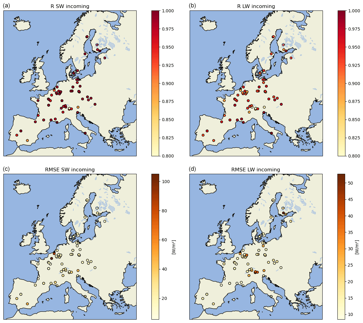
Figure 1 Validation of SW_in and LW_in from LSAF across Europe for 2018–2019 in terms of Pearson's correlation coefficient (R, (a, b)) and the root-mean-squared error (RMSE, (c, d)).

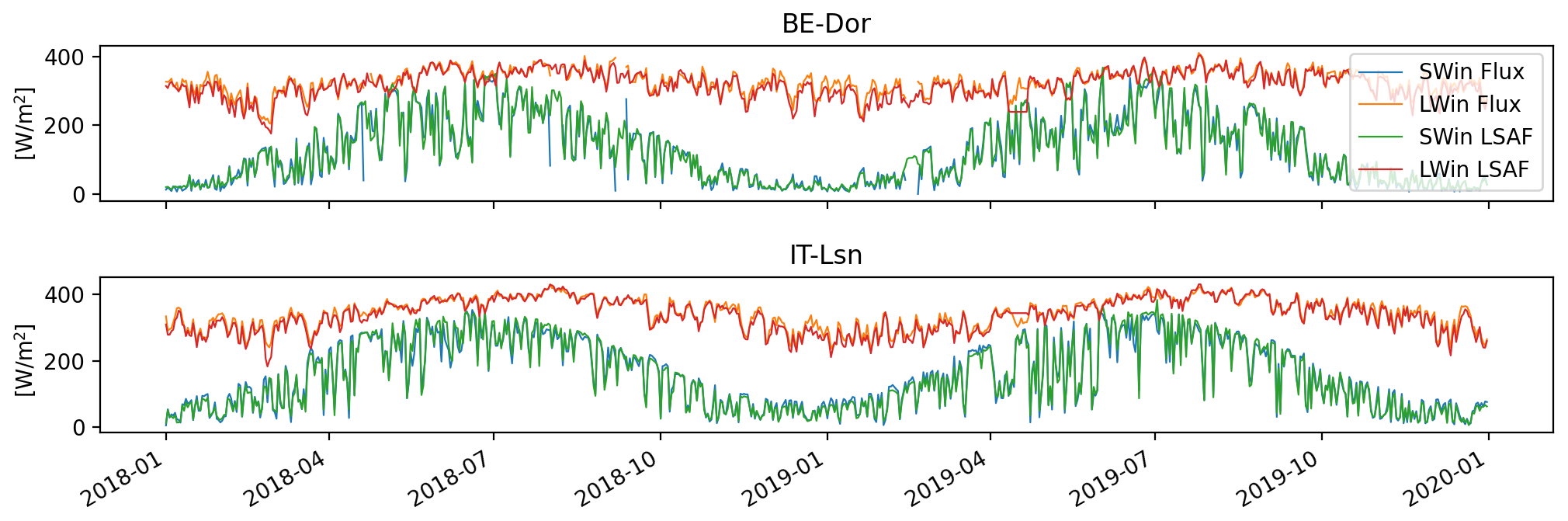
Figure 2 Daily averages of SW_in and LW_in from LSAF and the ground truth for two stations, BE-Dor and IT-LSN.

Additional seasonal validation statistics for the incoming radiation components are given in the Appendix (see boxplots in Figs. B1 and B3). In summary, for SW_in, R is consistently high throughout the year, albeit with a higher spread of values for the individual seasons (given that the overall seasonal amplitude has a lesser impact). The RMSE varies slightly from season to season, with the highest values occurring in summer (April/May/June and July/August/September). This coincides with generally much higher radiation values during these months. In terms of the mean square percentage error (MSPE), the error is highest in the winter months. A slight bias of 5 W m⁻² is observed throughout the year, although it is less pronounced during winter and spring. Validation metrics for different land cover types are also given (Figs. B2 and B4), with the ESA CCI land-cover product (Harper et al., 2023) being used, as its spatial resolution (300 m) is more consistent with the spatial resolution of the data products developed here than the land cover information provided by the FLUXNET sites. For LW_in (Figs. B2 and B4), R again shows a higher spread for the individual seasons than for the entire study period. RMSE is highest in spring. In terms of land cover, all land cover types show high values for R, whereas the flooded/brackish/water areas clearly show degraded performance for RMSE, RMSPE and bias (Fig. B4).

4.2 Land surface temperature

Extensive validation of the LSAF and Sentinel-3 LST products has already been performed. Both have an average accuracy below 1.5 K, although it varies across space and time. Our goal is to combine their individual strengths in terms of spatial and temporal resolution to obtain an enhanced representation of landscape heterogeneity. For an in-depth quantitative validation of the Sentinel-3 LST product, we refer the reader to Pérez-Planells et al. (2021). The LSAF LST products were validated by Trigo et al. (2008a), Göttsche et al. (2013), Göttsche et al. (2016), Martins et al. (2019) and Trigo et al. (2021). Here, the validation against in situ data is carried out not directly on LST but on LW_out – see Sect. 3.3. This is because LST validation data are limited and thus a validation using LW_out ground truth measurements is much more comprehensive. Furthermore, the developed LST product primarily serves the purpose of enabling a spatially downscaled LW_out product for the final calculation of the SNR.

Figure 3 shows a comparison between the mean annual LST for 2018–2019 from LSAF and the merged LSAF/Sentinel-3 LST for two regions in Europe. The downscaled LST product shows significantly more spatial detail, especially in heterogeneous or topographically complex areas such as the Central System in Madrid (top row) or the Rhine Valley and its surrounding mountainous areas (bottom row). Instead of the 2018–2019 LST average, Fig. 4 shows the original LSAF LST and the downscaled LST product for 30 June 2018. This day was chosen for no particular reason and is representative of other dates.

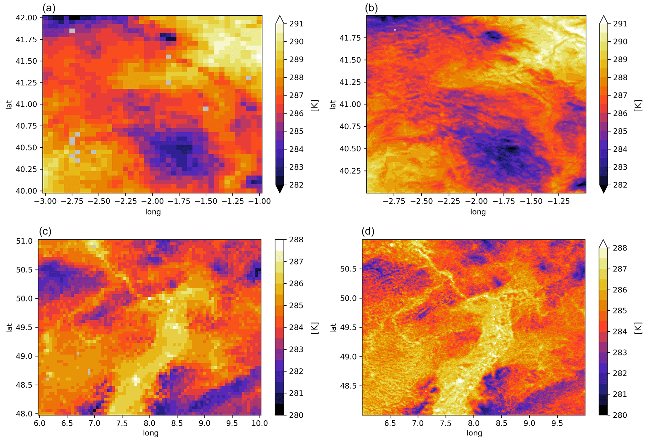
Figure 3 Mean LSAF LST (a, c) and merged LSAF/Sentinel-3 LST (b, d) for 2018–2019, showing a part of the Iberian Peninsula (a, b) and the southern Rhine Valley (c, d).

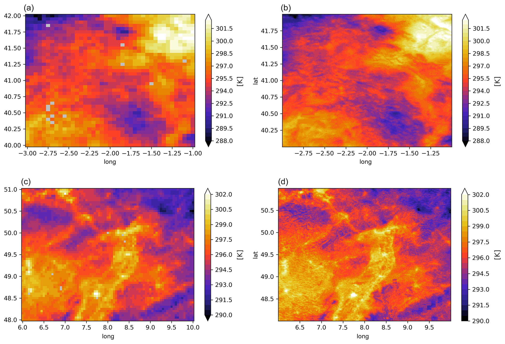
Figure 4 LSAF LST (a, c) and merged LSAF/Sentinel 3 LST (b, d) for 30th June 2018, showing the centre of the Iberian Peninsula (a, b) and the southern Rhine Valley (c, d).

4.3 Land surface albedo

Figure 5 shows the 2018–2019 mean albedo from LSAF and from the downscaled albedo product across parts of the Rhine Valley, as well as the values for a single day, analogous to the LST in Figs. 3–4. The effect of the downscaling in enhancing the spatial detail in the LSAF albedo retrievals based on PROBA-V retrievals is evident; see (e.g.) the distinct areas of low albedo surrounding the Rhine Valley that are covered by forests and the higher-albedo areas within the valley.

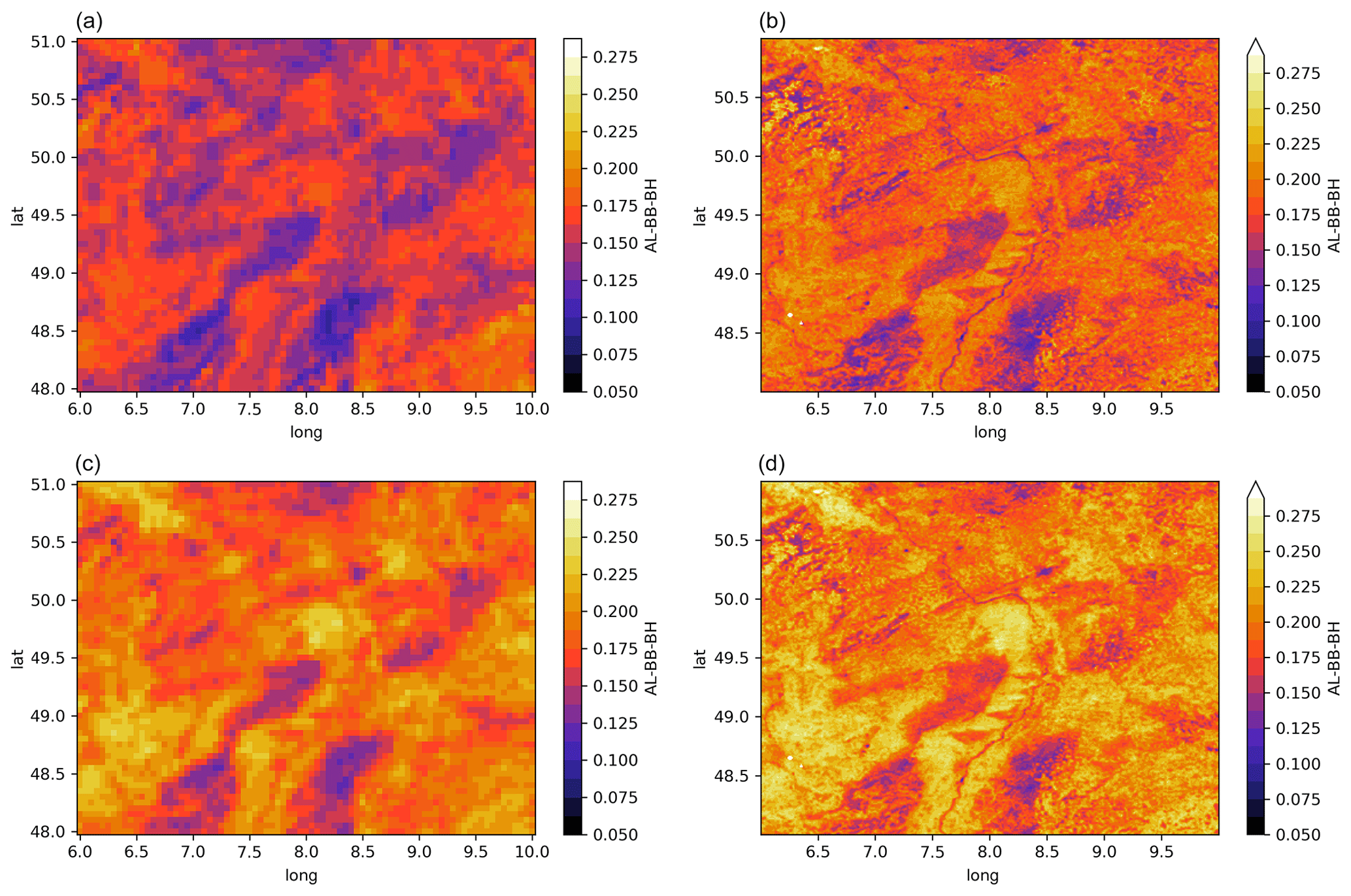
Figure 5 Mean albedo from LSAF (a) and the downscaled dataset (b) for 2018–2019, as well as the retrievals for the 30 June 2018 for LSAF (c) and the downscaled albedo product (d). The maps depict the southern Rhine Valley, with the river flowing from south to north through the centre of the landscape shown and then to the north-west.

4.4 Outgoing radiation fluxes

SW_out estimates resulting from combining LSAF SW_in with either LSAF α or with the downscaled α dataset are validated against in situ data. SW_out, obtained using either the LSAF LST or the downscaled LST product, is also compared against in situ data. This validation therefore shows to what extent the downscaling of SW_out and LW_out in combination with emissivity data from LSAF influences the accuracy, not only the spatial detail, as shown in Sect. 4.2 and 4.3.

On average, the RMSEs for both SW_out and LW_out are lower when compared to those obtained using data from LSAF only, with a mean of 17.1 W m⁻² vs 17.8 W m⁻² for SW_out and 11.4 W m⁻² vs 11.04 W m⁻² for LW_out). Figure 6 shows the distribution of the RMSE across the available sites for the 2018–2019 period for SW_out and LW_out. The absolute values for the RMSE of LSAF as well as the difference from the downscaled products are included.

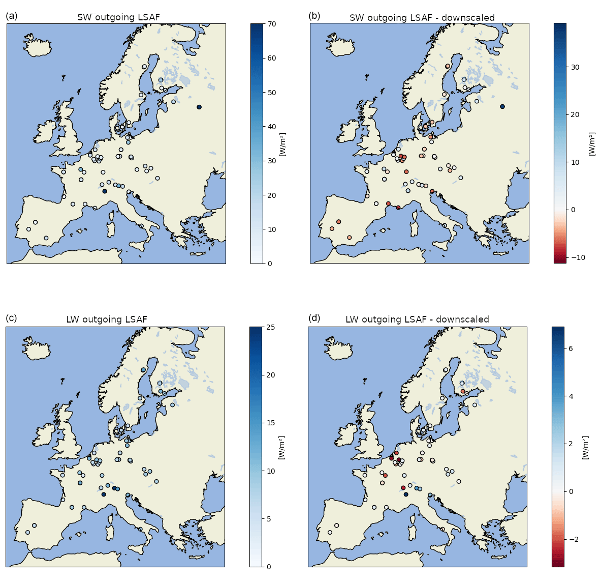
Figure 6 Validation of SW_out (a, b) and LW_out (c, d) in terms of RMSE based on LSAF only (a, c) and the difference from the downscaled products (b, d); blue colours in panels (b, d) indicate better performance of the downscaled products.

Figure 7 shows the R, MSE, MSPE and bias for LSAF and the downscaled product across the different CCI land cover types. For R, both SW_out and LW_out show lower performance for the water-related land cover types. For MSE, the same is true only for SW_out, and tree-covered areas show a slight positive bias here, whereas the other land cover types are on average negatively biased. For LW_out, the bias seems less pronounced and the median land-cover values are generally above or close to 0.

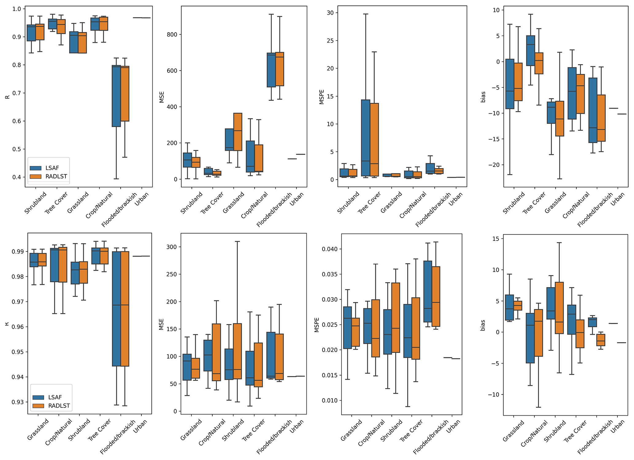
Figure 7 Validation of SW_out (top) and LW_out (bottom) radiation in terms of R, RMSE, RMSPE and bias for LSAF only and the downscaled product across different land cover types.

For a complete picture, the validation metrics are also calculated seasonally (see Fig. C1 in Appendix C). Seasonal patterns are most pronounced for the RMSPE in SW_out, which is significantly higher during the winter months. One explanation is that the calculation relies on accurate albedo values but their retrieval is especially challenging in winter due to cloud cover. Valid albedo values are linearly interpolated to fill in the data gaps, and snow cover will have an especially significant impact. High errors for SW_out in snow cover conditions can thus be expected.

4.5 Surface net radiation

Finally, the downscaled SNR dataset resulting from the hourly SW_in and LW_in as well as the downscaled hourly SW_out and LW_out is validated against the available in situ data at daily timescales. On average, the downscaled product has a RMSE of 22.53 W m⁻² vs 23.5 W m⁻² for the MSG-only product. Figure 9 shows the distribution of RMSE values across the study domain. A time series for a single example site is shown in Fig. 10. We also analyse how the downscaled SNR product performs under cloudy and clear-sky conditions. Clear-sky conditions were assumed for the daily SNR product when more than 12 h of LSAF clear-sky LST observations were available. Figure 8 shows that for clear-sky conditions, both R and the bias are improved when compared to cloudy conditions. The RMSE is slightly higher for clear-sky conditions, which is likely linked to seasonality, as clear-sky conditions are more common during summer, when the SNR values are also higher.

Figure 8 Validation of the SNR for cloudy and clear-sky days in terms of R, RMSE and bias.

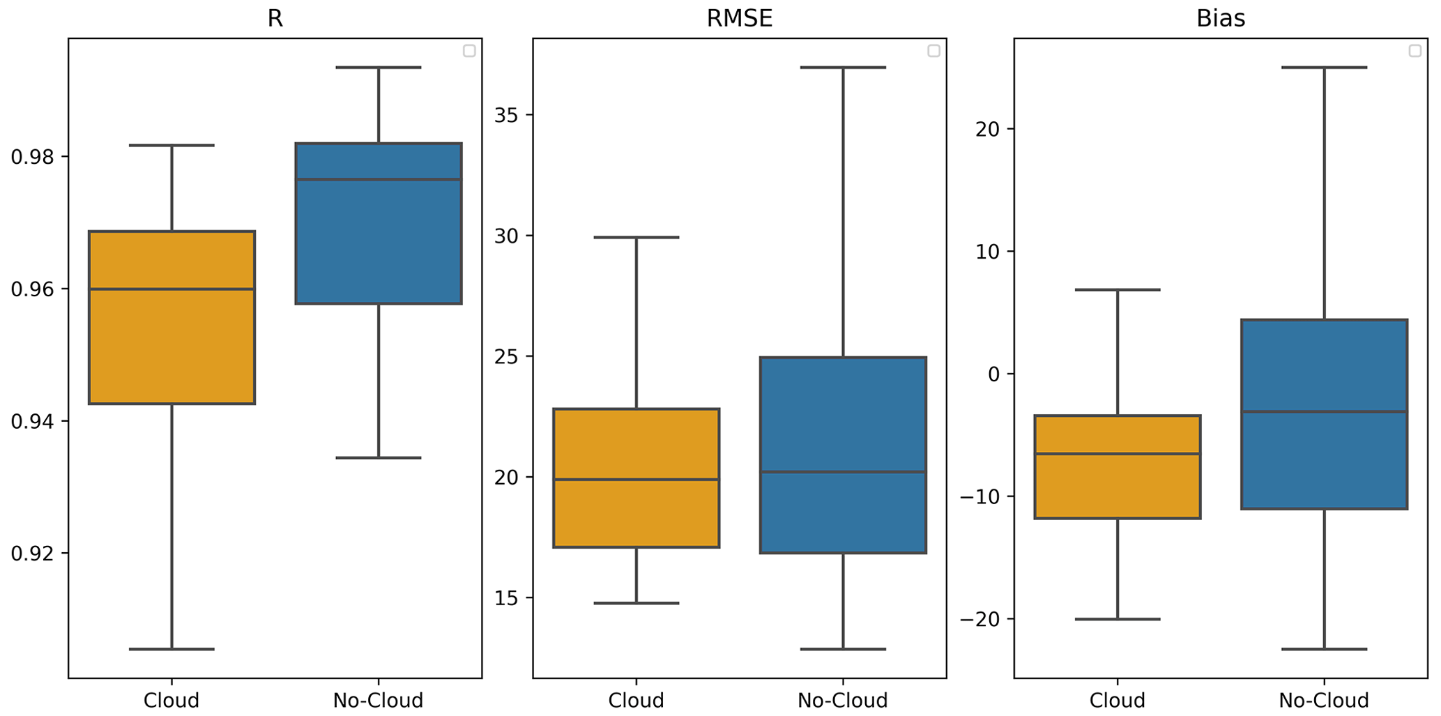
Figure 11 shows the SNR validation for the different CCI land-cover types for a LSAF-only-based SNR as well as the downscaled product. The figure also includes performance metrics for the ERA5-Land product (Muñoz-Sabater et al., 2021), which were included to give some context. R is generally high for all products (ca. 0.95) at all sites with the exception of the sites with land cover affected by water. There, ERA5-Land outperforms the LSAF and downscaled SNR product in terms of R, likely due to a sub-optimal treatment of these areas in the processing of the input products. In terms of MSE, ERA5-Land again outperforms the other products for water-affected land cover. However, for the other land cover classes, the LSAF SNR and downscaled products perform better, with the downscaled dataset showing the lowest MSE values. In terms of bias, ERA5-Land shows the best performance, followed by the downscaled product, which outperforms the LSAF-only SNR.

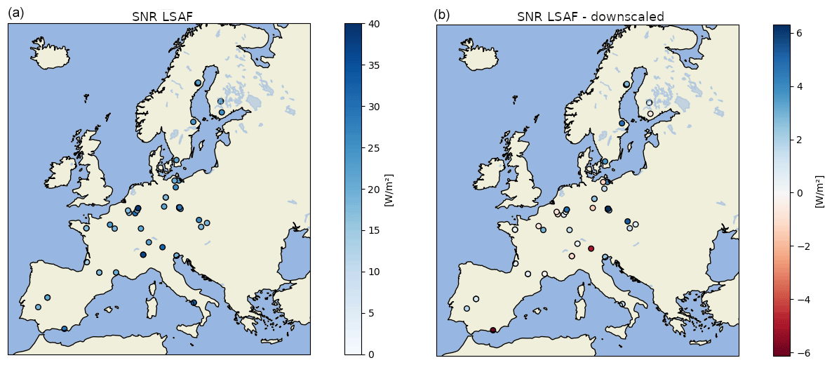
Figure 9 Validation of the SNR in terms of RMSE using LSAF only (a) and the difference from the downscaled product (b); blue colours in (b) indicate better performance of the downscaled product.

Figure 10 Daily averages of downscaled SNR, LSAF SNR and ground truth for the site IT-Lsn.

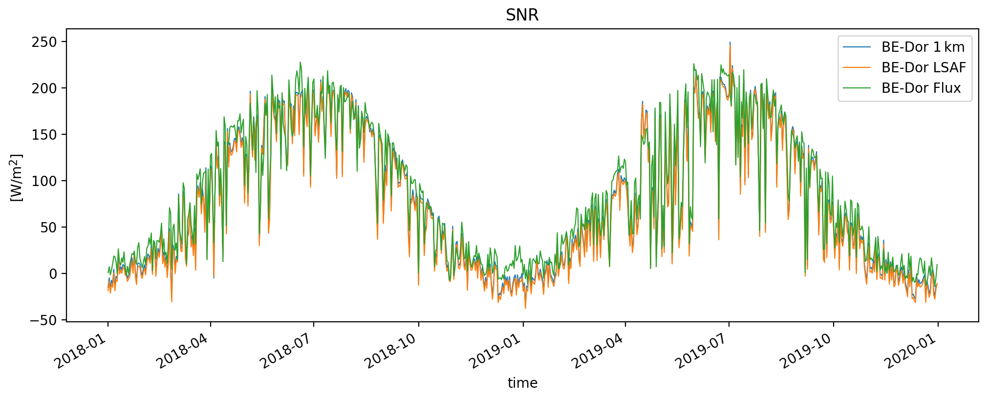
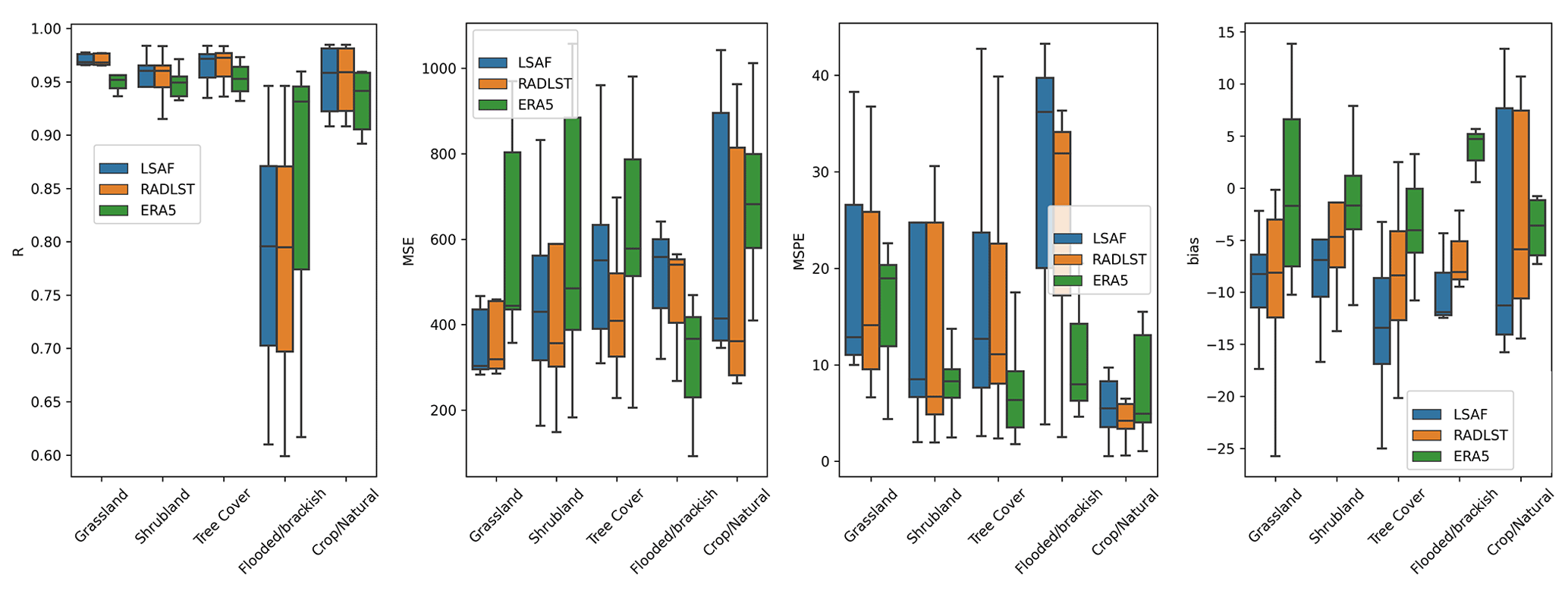
Figure 11 Validation of the SNR for different CCI land-cover types in terms of R, MSE, MSPE and bias.

For the SNR products, we also carry out a seasonal analysis. The results of this are shown in Figs. D1 and D2 in boxplot form (see Appendix). Tables E1 and E2 list all performance metrics for the entire study period as well as seasonally. For the entire 2018–2019 period, R is very similar for both datasets, with R=0.93 for the downscaled product and R=0.92 for ERA5-Land. In comparison to ERA5-Land, the downscaled product has a RMSE of 22.53 vs 25.7 W m⁻². The average bias is lower for ERA5-Land, with −1.56 vs −6.83 W m⁻².

The downscaled product shows better performance in spring (AMJ) with R=0.91 vs R=0.83 and summer (JAS) with R=0.93 vs R=0.86. The same holds true for RMSE with 27.58 and 22.18 W m⁻² for AMJ and JAS respectively, compared to 34.79 and 29.37 W m⁻².

Figure 12 shows, as an example, the SNR for the downscaled product and ERA5-Land for 30 June over an area of western Europe. The increase in spatial resolution and therefore landscape details is clearly visible. The downscaled dataset shows both higher and lower values than ERA5-Land as it is able to resolve finer land surface features due to the high-resolution merged LST and albedo inputs.

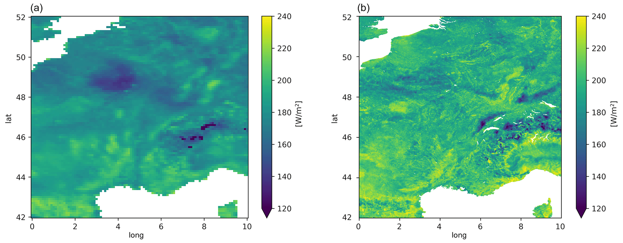
Figure 12 The SNR from ERA5-Land (a) and the downscaled dataset (b) for 30 June 2018. The maps shown depict a large part of western Europe covering France, Germany and Italy. Data gaps around lakes and shorelines due to the relatively coarse resolution of the LSAF inputs have been filled through bilinear interpolation and a 1 km water mask has been applied.

5 Discussion

The methodology described and validated above to produce the gap-free all-sky SNR at 1 km resolution relies on producing gap-free 1 km SW_out and LW_out estimates. The methodology used to produce SW_out, namely bias correction, is relatively straightforward. The more complex multi-stage approach taken for the all-sky LST estimates, which are required to compute LW_out, is discussed in some more detail here with regards to similar studies. Some further remarks on other available SNR products, a comparison of the SNR product created here to ERA5-Land, and the validation of the individual radiation components follow.

Examples of other gap-free LST datasets which have recently been developed are given by Shiff et al. (2021), Xu and Cheng (2021), Jia et al. (2022) and Wu et al. (2023). The approach taken by Shiff et al. (2021) was to merge the clear-sky 1 km MODIS LST with the 0.2^∘ modelled air temperature provided by the National Center for Environmental Prediction (NCEP) from the Coupled Forecast System Model version 2 (CFSv2) system. This was done by extracting the underlying seasonal behaviour from both input datasets by temporal Fourier analysis and subsequently adding the CSFv2 anomalies to the MODIS climatology on days for which no clear-sky MODIS LST observation is available. Xu and Cheng (2021) demonstrated a multi-step approach based on infrared Advanced Microwave Scanning Radiometer 2 (AMSR2) brightness temperatures, MODIS LST as well as MODIS-based ancillary datasets and elevation data. First, the land surface temperature is retrieved from all the above datasets at 0.1^∘ spatial resolution. This LST dataset is then downscaled from 0.1^∘ resolution to 0.01^∘ resolution by using the elevation data and MODIS NDVI. Clear-sky MODIS LST data and the retrieved all-sky LST data are then bias corrected, allowing for the temporal gap filling of the clear-sky LST retrievals. Finally, the 0.1^∘ LST retrievals based on AMSR2 are assimilated into the merged 0.01^∘ LST dataset by applying a multi-resolution Kalman filtering approach. Jia et al. (2022) have produced all-sky diurnal hourly LST estimates at 2 km spatial resolution based on the surface energy balance. The three-step approach is based on constructing a spatiotemporal dynamic model of LST from ERA5 in which clear-sky LST data from the Advanced Baseline Imager (ABI) are assimilated. As a final step, the gap-free LST record is updated by superimposing diurnal cloud effects using satellite radiation products. Wu et al. (2023) have tested an approach to produce very-high-resolution, 100 m gap-free LST data from a single Landsat 8 acquisition by training a random forest algorithm with the Landsat-derived LST and ancillary variables, e.g. land cover, population density and elevation. The LST merging methodology presented in this paper shares some of the elements of the above-mentioned studies, i.e. primarily the bias correction of the coarse-scale LSAF LST observations towards Sentinel-3 (see Sect. 3.3), as well as a Kalman filtering approach. An in-depth validation and quantitative inter-comparison of the above-mentioned products was not the aim of this study presented here. We argue, however, that on a theoretical basis, the methodology proposed here has some advantages. Most of the above-mentioned approaches rely on input data with a coarser spatial resolution. Shiff et al. (2021) and Jia et al. (2022), for instance, use air temperature data at a 0.2^∘ resolution or ERA5 with an approximately 31 km spatial resolution. Both these datasets are also model output, albeit from data assimilation systems taking a multitude of observations into account. The coarsest spatial resolution of the input datasets used in the methodology presented here are the LSAF geostationary retrievals, with a pixel size of ca. 5–7 km, depending on the latitude. While, in particular, the LSAF all-sky retrievals are also based on modelling and require ancillary information, they are optimised for the retrieval of the single target variable at high accuracy. They are also available hourly, like ERA5, whereas e.g. Landsat 8, used by Wu et al. (2023), is only available every few days, depending on the cloud cover. Furthermore, our approach does not rely on using ancillary variables which are not directly linked to the physical processes to statistically downscale the input products, as is for example done in Wu et al. (2023) by using population density. One of the drawbacks of the methodology presented here is the lack of a dynamic temporal model which is able to propagate assimilation updates (provided by the 1 km LST retrievals from Sentinel-3) over time, which has been achieved by Jia et al. (2022). Here we thus apply the same update from when a Sentinel-3 observation is available to the subsequent time steps until the next Sentinel-3 observation is available. An additional drawback is that e.g. ERA5 and NCEP are globally available datasets, and the use of MODIS LST retrievals allows for the production of long time series. In contrast, LSAF is limited to North Africa and Europe, and Sentinel-3 was only launched in 2016. The approach can, however, be transferred to other regions by substituting LSAF with other geostationary retrievals and using MODIS instead of or in addition to Sentinel-3 to allow for an extension of the time series.

In terms of the calculation of the daily all-sky surface net radiation dataset, we argue that the approach taken here is the most straightforward, as it is based on the underlying physical principles of the individual radiation components. This is in contrast to studies presenting methods to produce net radiation at a similar temporal and spatial resolution which exploit statistical relationships between some well-observed components (e.g. incoming radiation components from a satellite) and ancillary information (e.g. land cover or NDVI) or modelled variables. Xu et al. (2022), for example, train a convolutional neural network using net radiation from a selection of in situ measurements, modern-era retrospective analysis for research and applications, version 2 (MERRA-2) reanalysis and advanced very high resolution radiometer (AVHRR) top-of-atmosphere (TOA) data. Jiang et al. (2023) presented two algorithms based on a random forest to downscale the GLASS net radiation product, either by exploiting the relationship between net radiation and short-wave radiation as well as ancillary information, including that from ground measurements, or by linking net radiation to TOA observations from the Landsat satellites and ancillary information. The GLASS algorithm itself is based on the multivariate adaptive regression splines (MARS) model trained with remotely sensed incoming radiation, NDVI and albedo as well as mostly MERRA-2 meteorological variables (Jiang et al., 2016). While such downscaling methodologies can work very well, and we need to note that no quantitative comparison is performed here, they rely on training a model which establishes a statistical relationship between the different input variables. These data-driven approaches are very sensitive to the training data and e.g. the spatial or temporal domain for which such a model is established. Hence, a globally trained model might not capture locally specific conditions or provide accurate output for time periods not considered for the training. As in situ training data are often the limiting factor, established statistical relationships might also only be valid for these specific sites, and avoiding model overfitting can be very challenging. It can thus be beneficial if in situ measurements are solely used for the validation of a methodology rather than the development itself. Another methodology to produce hourly surface solar radiation at 5 km spatial resolution was developed by Tang et al. (2016). In the two-step approach, hourly cloud parameters are estimated with a neural network by combining cloud products from MODIS with high-temporal-resolution TOA radiance data from the geostationary Multifunctional Transport Satellite (MTSAT). Subsequently, the cloud information and other auxiliary information are combined in a radiative transfer model to retrieve the surface net radiation. Conceptually, although it estimates surface radiation primarily based on cloud properties, it is similar to the approach presented here in exploiting the advantages of geostationary and polar-orbiting satellite measurements and being more physically based. An overview of some further approaches to produce surface net radiation products is also given by Tang et al. (2016).

We need to state that in this paper we make no accuracy comparisons between the different approaches mentioned above. Also, in terms of ancillary variables, this study indirectly relies on these through the use of the chosen input products. The retrieval of the LST, for instance, especially in cloudy conditions, relies on modelled processes requiring information such as the vegetation phenology. In terms of the validation of the produced SNR product and the individual radiation components, we also acknowledge that the in situ measurements have an error (the difference from the “truth” at the local scale that they sample), but that the pixel to local representativeness error, i.e. the difference between the pixel truth that we aim for and the local truth at the smaller tower footprint, is much larger. Unfortunately, we cannot solve this issue, but we argue that using as many stations as possible benefits the validation, particularly within pixels where the spatial heterogeneity is very large. Finally, by relying on input products that directly represent components of the surface radiation balance, any future enhancements in the source products should directly lead to improvements in future releases of the 1 km SNR dataset.

6 Data availability

The daily SNR and LST datasets for 2018–2019 are available for scientific use under https://doi.org/10.5281/zenodo.8332222/ https://doi.org/10.5281/zenodo.8332128 as netcdf files (RNETdaily_lon_lat.nc and LSTdaily_lon_lat.nc); see Rains (2023a) and Rains (2023b). The spatial domain covered by the product is −11.5 to 26.5^∘ longitude and 35 to 71^∘ latitude.

7 Conclusions

Surface net radiation is a key input variable for many land surface and hydrological models. With increased efforts to simulate land surface processes at higher spatial resolution, the lack of high-resolution gap-free SNR data is an issue. The heterogeneity of the model output is then primarily driven by land surface properties for which high-resolution datasets are more frequently available (e.g. soil texture, vegetation phenology). In this paper, we have presented a methodology to systematically combine the advantages of frequent geostationary LST and radiation observations, enhanced with modelled data when cloud cover inhibits the direct retrieval, with LST and albedo retrievals from polar-orbiting satellites at high spatial resolution. The resulting gap-free net radiation dataset, as well as the intermediate all-sky LST dataset, for 2018–2019 across Europe uses operationally available input datasets, which opens up the possibility of updating the data on a close to near-real-time basis. Based on the surface energy balance, and by optimising each radiation component individually using input datasets that already have a high accuracy, some improvements are achieved in addition to a substantial increase in spatial heterogeneity and representativeness.

While a gap-free LST dataset was developed within this study, the validation of the dataset was carried out indirectly based on LW_out measurements. This served the purpose of the study: to ultimately create a SNR dataset.

Conceptually, one of the advantages of the LST merging methodology developed here within the overall scope of producing net radiation is its reliance on one of the LST input products provided by LSAF, thus making the approach more consistent, as the incoming radiation components are also LSAF products. The use of Sentinel-3 SLSTR emissivity maps when computing the outgoing long-wave radiation LW_out should be considered in future product updates to make the methodology even more consistent. In addition, the presented results are based on the use of LST retrievals from the Sentinel-3A satellite, and data from Sentinel-3B should be incorporated in the future. Also, the use of Sentinel-3-based albedo instead of PROBA-V should be explored. A limitation of the downscaling methodology is that in the assimilation step performed after the bias correction of LSAF LST towards Sentinel-3, there is no dynamic model to propagate the updates from the Sentinel-3 LST assimilation at the daytime or nighttime overpass time to the subsequent hours. To address this issue, we applied equivalent updates to the subsequent hourly LSAF observations separately for temporal daytime/nighttime windows. Alternative approaches – such as the attenuation of the assimilation impact over time – could be explored based on a more in-depth analysis of the diurnal cycle. While the validation presented here concentrated on daily aggregates, the availability of hourly LST and radiation products does make it possible to resolve the diurnal cycle, which can be a requirement for certain models.

In principle, the approach developed within this study can be extended to other areas where there are both geostationary and polar-orbiting observations, not necessarily the ones used for this study. The dataset presented here shall be updated in the future, as we consider it to be an ideal input dataset for high-resolution land surface applications, e.g. for the Global Land Evaporation Amsterdam Model (Martens et al., 2017).

Appendix A: In situ sites

Table A1 List of all in situ sites used for the validation of the radiation products throughout the paper. The columns show the station ID, name, geographic coordinates and IGBP land cover (when provided) as well as the measured variables at each site.

Appendix B: Incoming radiation fluxes

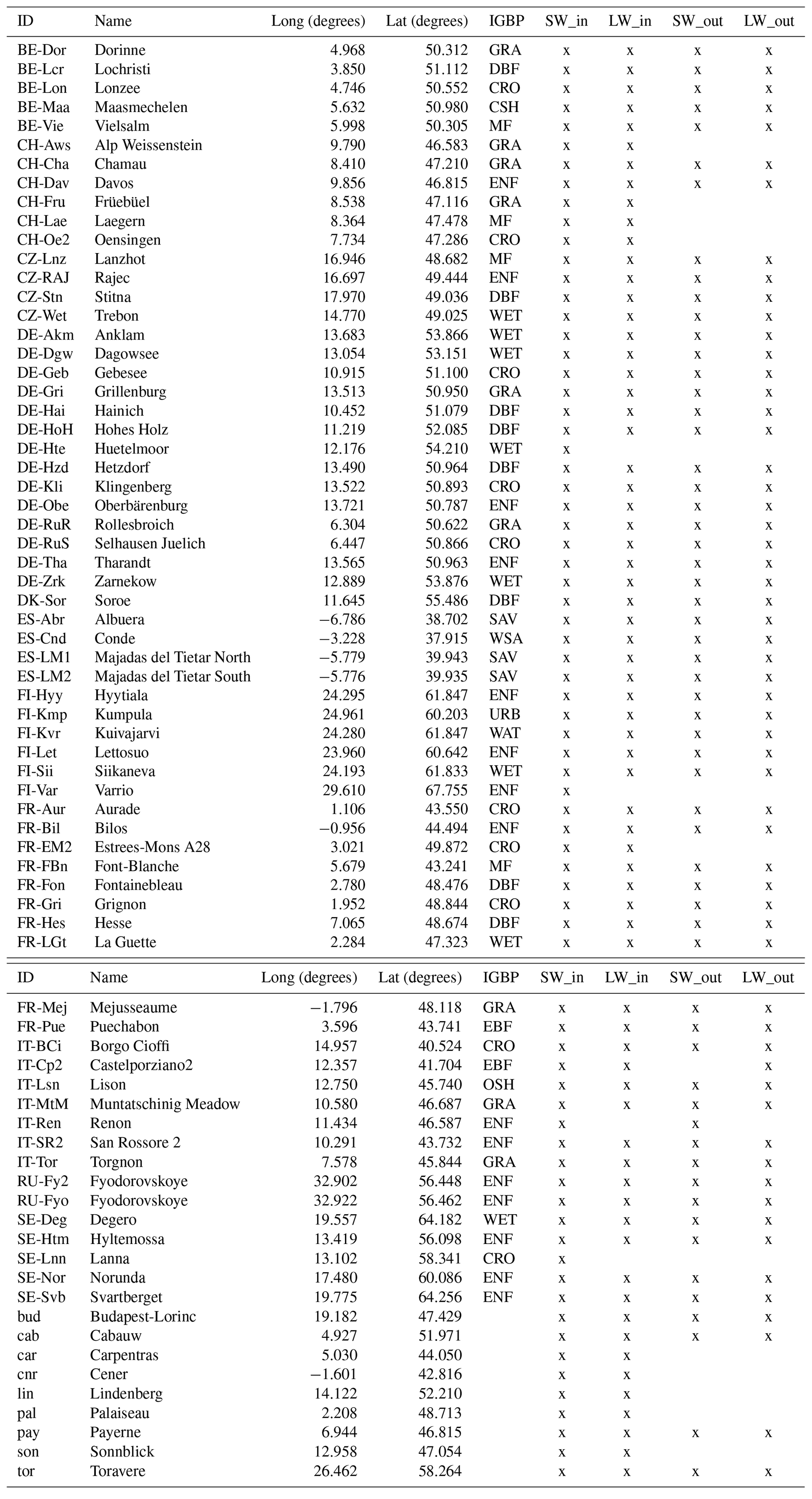
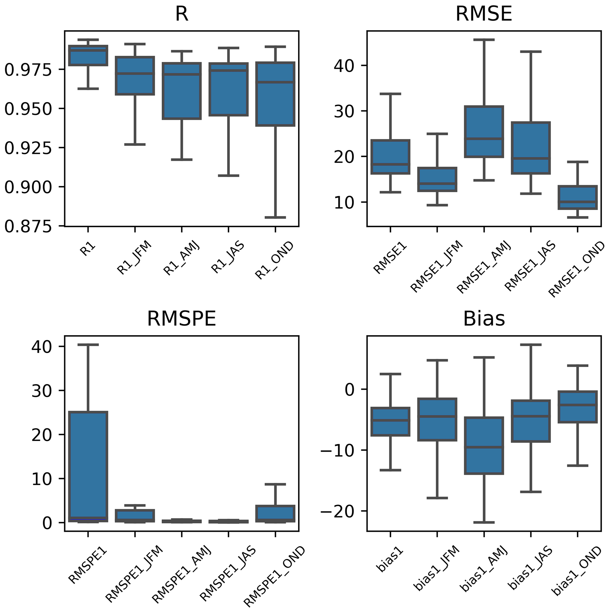
Figure B1 Validation of LSAF SW_in in terms of R, RMSE, RMSPE and bias for the entire period as well as seasonally.

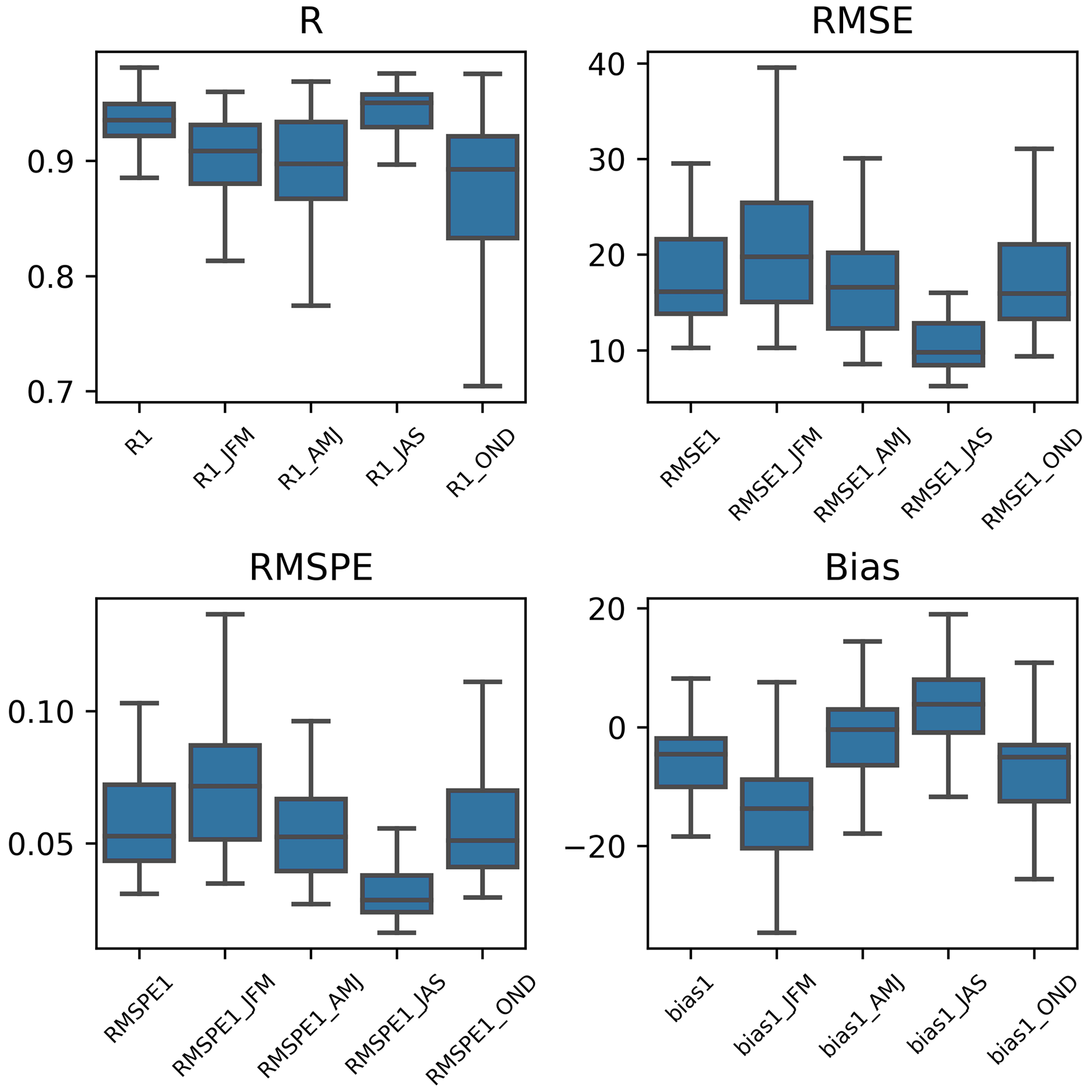
Figure B2 Validation of LSAF LW_in in terms of R, RMSE, RMSPE and bias for the entire period as well as seasonally.

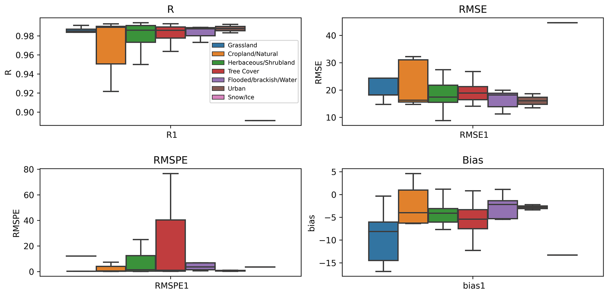
Figure B3 Validation of LSAF SW_in in terms of R, RMSE, RMSPE and bias for different land cover types.

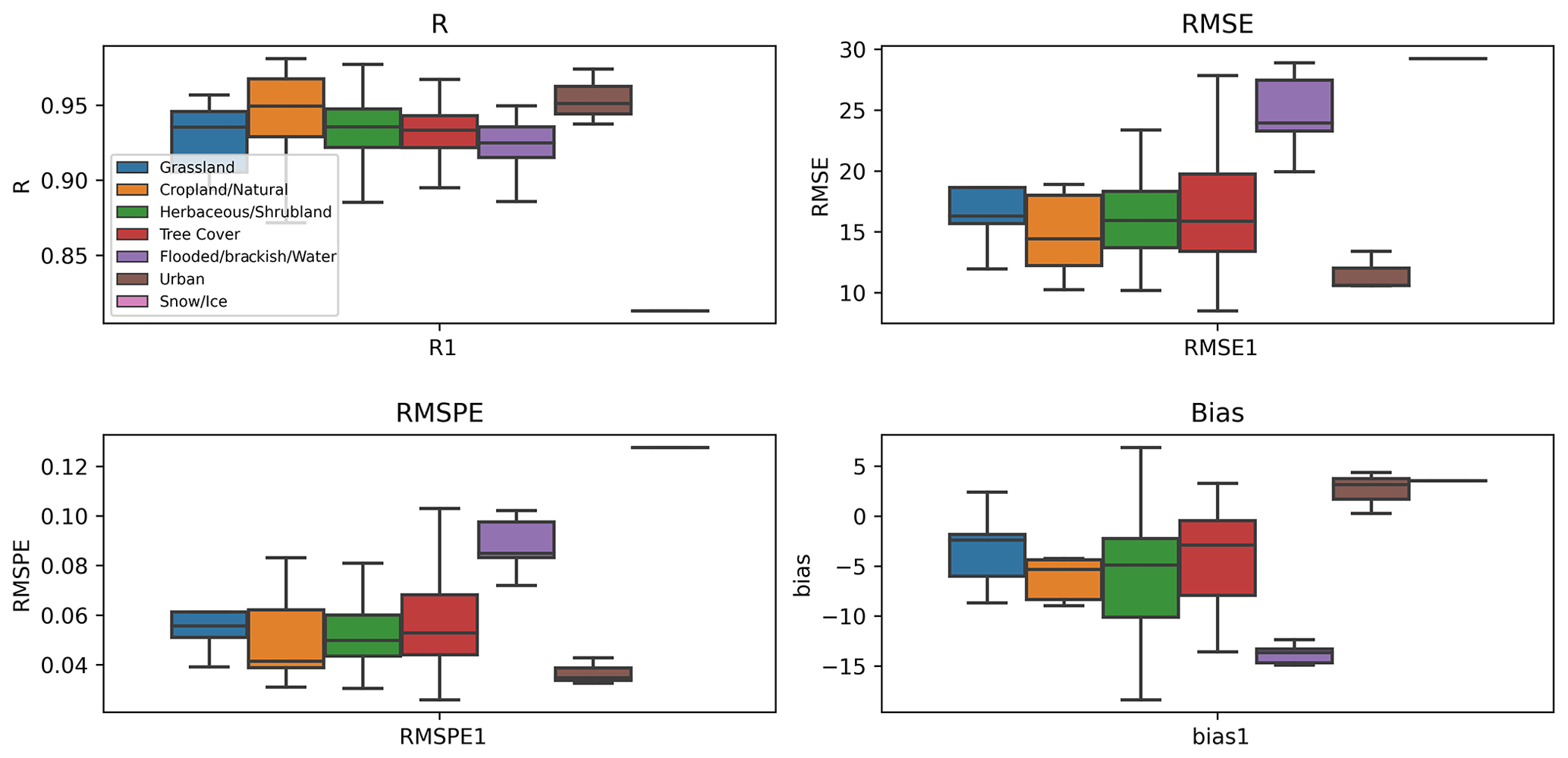
Figure B4 Validation of LSAF LW_in in terms of R, RMSE, RMSEP and bias for different land cover types.

Appendix C: Outgoing radiation fluxes

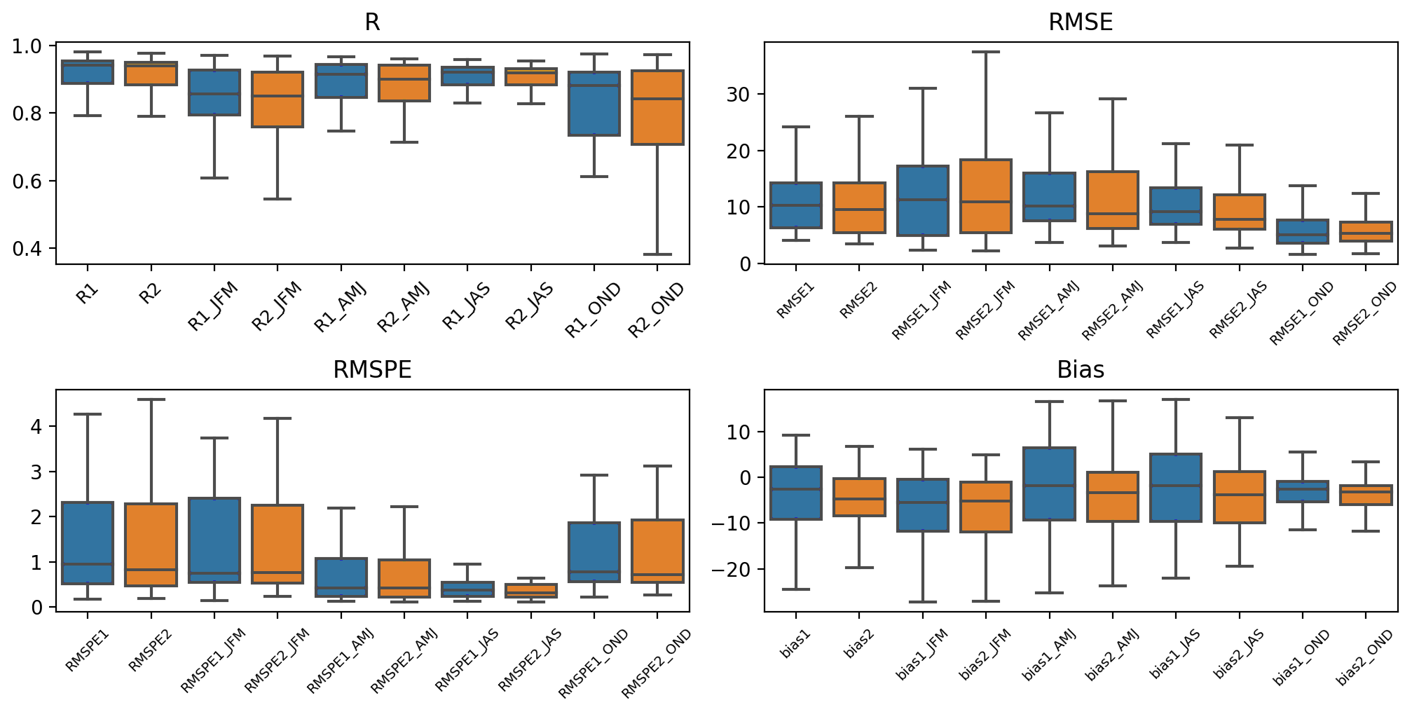
Figure C1 Validation of SW_out in terms of R, RMSE, RMSPE and bias using LSAF only (R1) and the downscaled product (R2) for the entire period as well as seasonally.

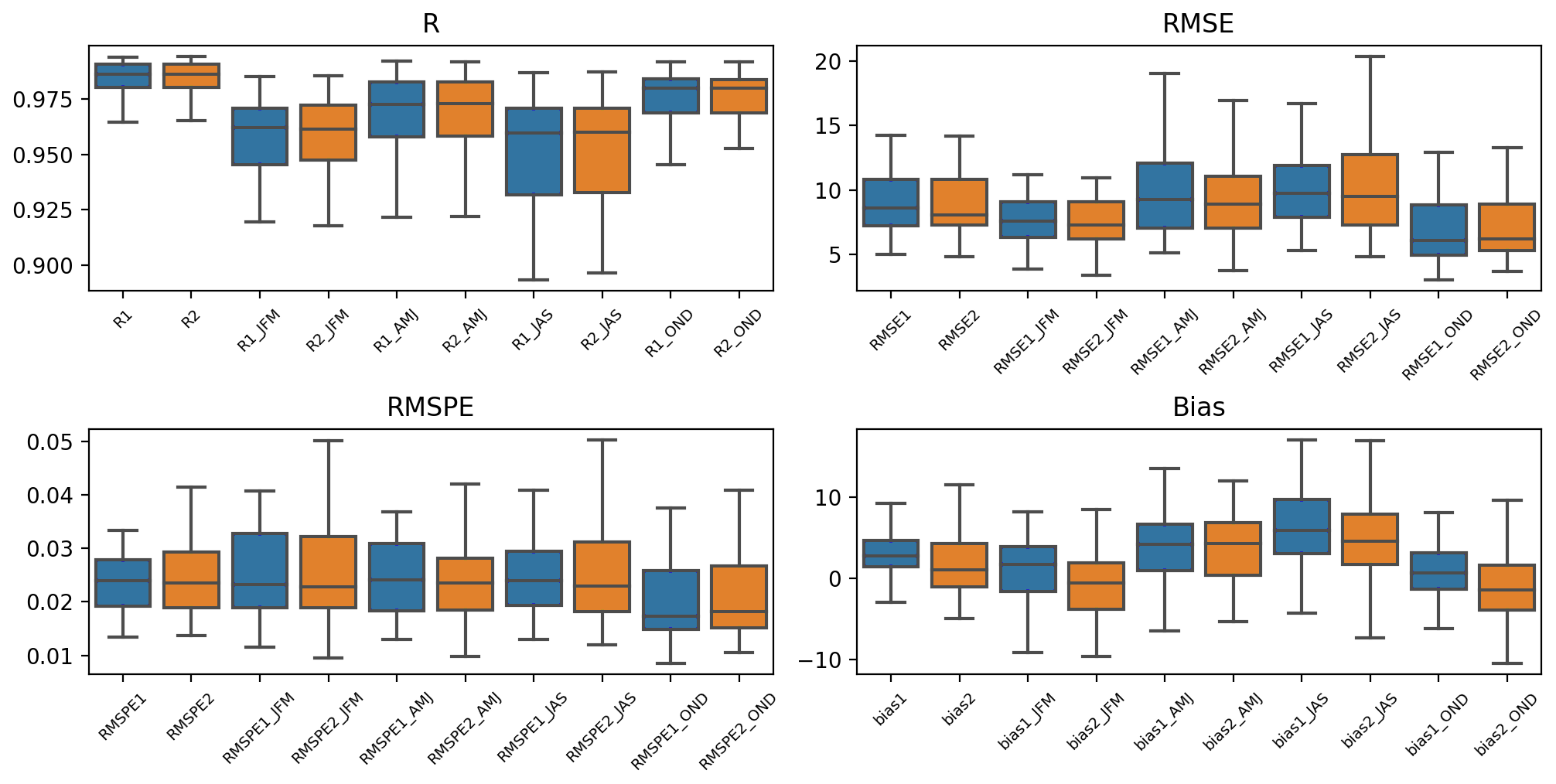
Figure C2 Validation of LW_out in terms of R, RMSE, RMSPE and bias using LSAF only (R1) and the the downscaled product (R2) for the entire period as well as seasonally.

Appendix D: Net radiation

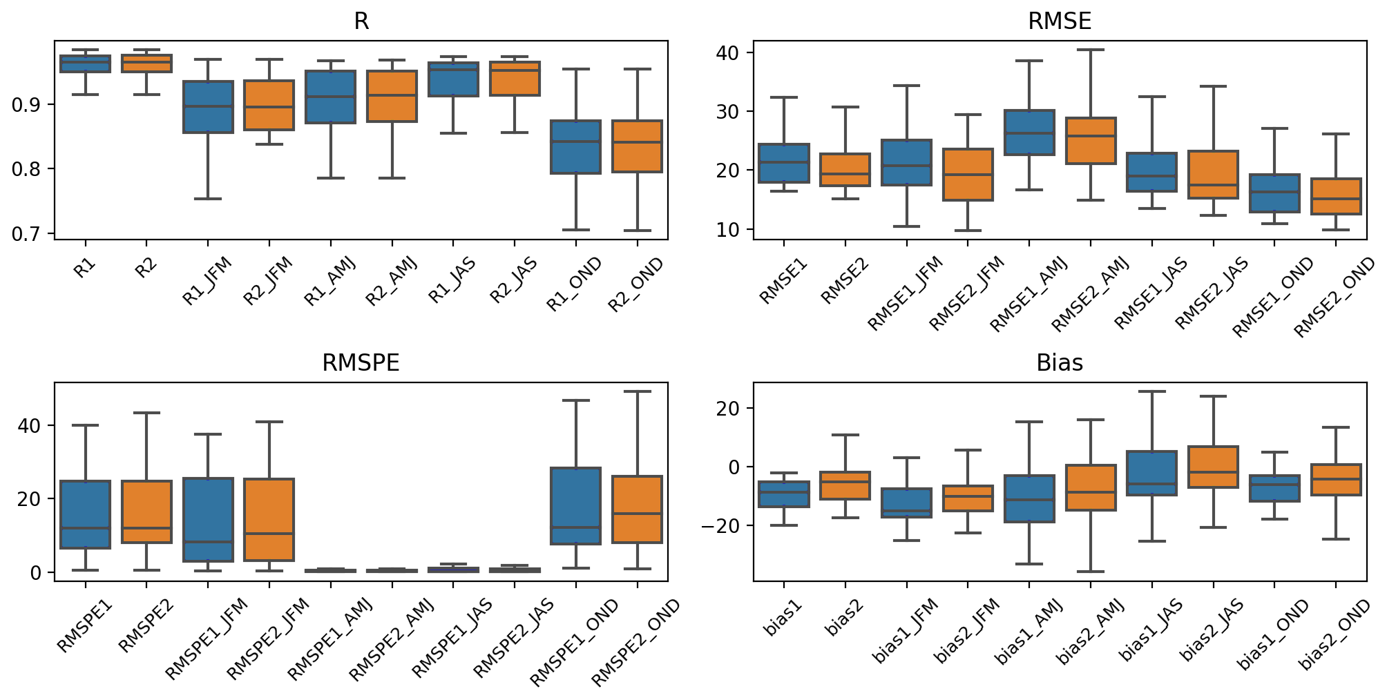
Figure D1 Validation of SNR in terms of R, RMSE, RMSPE and bias using LSAF only (R1) and the downscaled product (R2) for the entire period as well as seasonally.

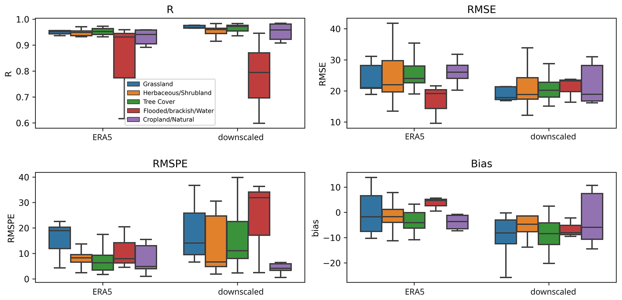
Figure D2 Validation of ERA5-Land and the downscaled net radiation product against in situ measurements in terms of R, RMSE, RMSEP and bias for different land cover types.

Appendix E: Overall validation statistics

Table E1 Performance metrics for radiation components for the 2018–2019 study period.

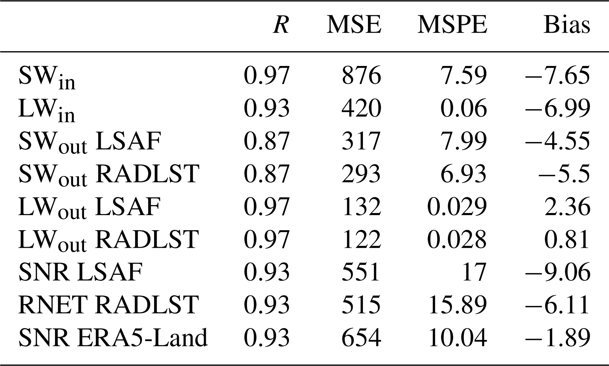
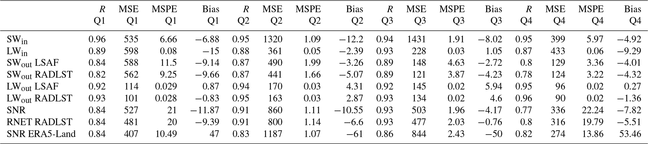
Table E2 Seasonal performance metrics for radiation components.

Appendix F: Downscaling of LSAF LST with Sentinel-3 LST

Some more detail is given here on the downscaling/merging of the LSAF with Sentinel-3-based LST retrievals described in Sect. 3.3. Figure F1 shows, as an example, the mean Sentinel-3 LST and its bias towards LSAF observations for daytime (10:00 am local time) observations. Across the domain, the bias is neither systematically negative nor positive, highlighting the generally high agreement between LSAF and Sentinel-3 observations, and it is more linked to geographic features. The UTC time of the underlying Sentinel-3 data is different for each pixel/day across the domain, and the LSAF data the bias is calculated against is thus a composite from different acquisition times. The Sentinel-3 observations are normalised to the on-the-hour Sentinel-3 mean overpass time per pixel to enable a more correct matchup between Sentinel-3 and LSAF (as the LSAF data are representative of on-the-hour data). This is done through linear interpolation using the LSAF LST difference between the full hour before and that after the exact overpass time of each Sentinel-3 observation. The bias correction is then performed between LSAF LST and the normalised Sentinel-3 observations for each pixel individually for the entire study period. A seasonal bias correction should be considered in the future.

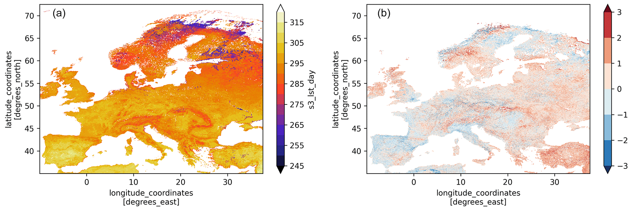
Figure F1 Mean LST of Sentinel-3 daytime (ca. 10:00 am) observations (a) and bias towards LSAF observations (b).

After the full bias correction of the hourly LSAF data, the normalised Sentinel-3 observations are assimilated into this time series for each pixel. The respective uncertainties of both Sentinel-3 and LSAF LST retrievals for each pixel/time step are therefore taken into account. Figure F2 shows the assimilation diagnostics for a single day as an example. The top row shows the Sentinel-3 LST retrieval (left), the uncertainty map of the Sentinel-3 observation (middle) and the uncertainty of the LSAF observations (right). The Kalman gain (bottom left) is based on the two uncertainties; a value of 1 corresponds to full trust in the Sentinel-3 observation, whereas 0 would result in no assimilation update. The difference, i.e. the innovation, between the Sentinel-3 observation and LSAF LST is shown in the lower middle plot. The increment, the actual update, is the innovation multiplied by the Kalman gain and is shown in the bottom right plot.

Figure F3 shows the 2018–2019 mean assimilation diagnostics for the daytime Sentinel-3 assimilation. The innovation (left) is fairly close to 0, showing that the bias correction results in the Sentinel-3 observations being, on average, spread evenly around the bias-corrected LSAF time series, as intended. The mean increment (middle), the actual correction applied to the LSAF estimates, shows similar spatial patterns. The mean Kalman gain is shown on the right.

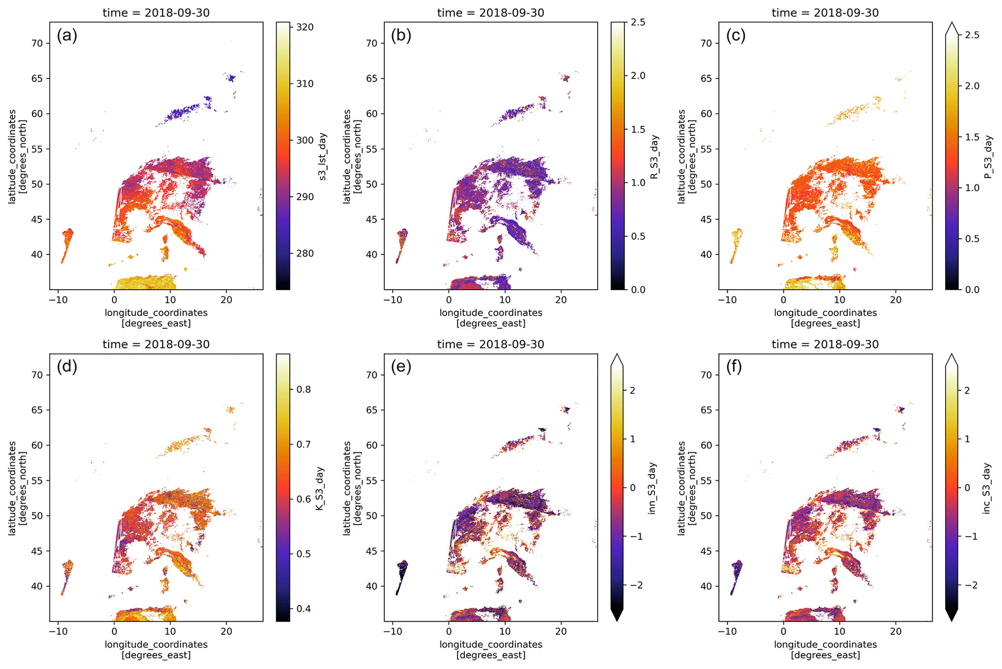
Figure F2 Sentinel-3 LST retrievals (a), uncertainty of Sentinel-3 LST retrievals (b), uncertainty of LSAF LST retrievals (c), Kalman gain (d), innovations (e) and increments (f).

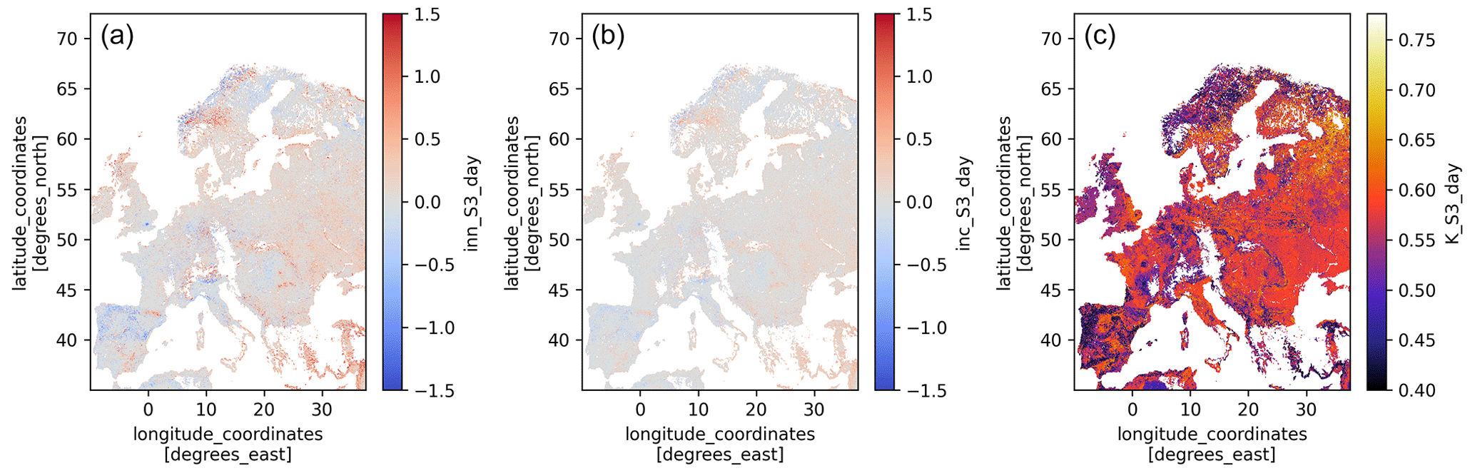
Figure F3 Mean innovation (a), increments (b) and Kalman gain (c) for daytime Sentinel-3 LST assimilation.