Annual maps of forest and evergreen forest in the contiguous United States during 2015–2017 from analyses of PALSAR-2 and Landsat images

Annual forest maps at a high spatial resolution are necessary for forest management and conservation. Large uncertainties remain in existing forest maps because of different forest definitions, satellite datasets, in situ training datasets, and mapping algorithms. In this study, we generated annual maps of forest and evergreen forest at a 30 m resolution in the contiguous United States (CONUS) during 2015–2017 by integrating microwave data (Phased Array type L-band Synthetic Aperture Radar – PALSAR-2) and optical data (Landsat) using knowledge-based algorithms. The resultant PALSAR-2/Landsat-based forest maps (PL-Forest) were compared with five major forest datasets from the CONUS: (1) the Landsat tree canopy cover from the Global Forest Watch dataset (GFW-Forest), (2) the Landsat Vegetation Continuous Field dataset (Landsat VCF-Forest), (3) the National Land Cover Database 2016 (NLCD-Forest), (4) the Japan Aerospace Exploration Agency forest maps (JAXA-Forest), and (5) the Forest Inventory and Analysis (FIA) data from the U.S. Department of Agriculture (USDA) Forest Service (FIA-Forest). The forest structure data (tree canopy height and canopy coverage) derived from the lidar observations of the Geoscience Laser Altimetry System (GLAS) on board NASA's Ice, Cloud, and land Elevation Satellite (ICESat-1) were used to assess the five forest cover datasets derived from satellite images. Using the forest definition of the Food and Agricultural Organization (FAO) of the United Nations, more forest pixels from the PL-Forest maps meet the FAO's forest definition than the GFW-Forest, Landsat VCF-Forest, and JAXA-Forest datasets. Forest area estimates from PL-Forest were close to those from the FIA-Forest statistics, higher than GFW-Forest and NLCD-Forest, and lower than Landsat VCF-Forest, which highlights the potential of using both the PL-Forest and FIA-Forest datasets to support the FAO's Global Forest Resources Assessment. Furthermore, the PALSAR-2/Landsat-based annual evergreen forest maps (PL-Evergreen Forest) showed reasonable consistency with the NLCD product. The comparison of the most widely used forest datasets offered insights to employ appropriate products for relevant research and management activities across local to regional and national scales. The datasets generated in this study are available at https://doi.org/10.6084/m9.figshare.21270261 (Wang, 2024). The improved annual maps of forest and evergreen forest at 30 m over the CONUS can be used to support forest management, conservation, and resource assessments.

1 Introduction

Forests cover approximately 30 % of Earth's land surface and have played major roles in regulating terrestrial carbon and water cycles (Harris et al., 2012; D'Almeida et al., 2007), influencing climate (Bonan, 2008; Peng et al., 2014), conserving biodiversity (Seto et al., 2012; Betts et al., 2017), and supplying forest products to humankind (Foley et al., 2005; Smith et al., 2018). The United States of America (USA) is covered by 310×10⁶ ha of forests and is the fourth largest forest country in the world, as estimated in the global forest resources assessment 2020 (FAO, 2020). Its forest biomes are dominated by the northwestern Rocky Mountains and Pacific coast evergreen forests, the eastern deciduous and mixed forests, and the southeastern coastal plain evergreen forests (CEC, 1997). The Forest Inventory and Analysis (FIA) program, managed by the U.S. Department of Agriculture (USDA) Forest Service, identified 142 forest types (by major tree species), which were aggregated into 28 forest groups across the USA (Ruefenacht et al., 2008). FIA has reported that the national forest area totals remain stable but that substantial changes have occurred at local and regional scales (Oswalt et al., 2019). In addition, extensive impacts of disturbance (e.g., wildfires, harvests, or insect outbreaks) and climate factors have increasingly been changing the forest structure, function, and species composition (Sexton et al., 2016; Mekonnen et al., 2019). It is crucial to generate timely and accurate annual forest maps at a high spatial resolution which can then be used to identify the forest area dynamics, assess the associated impacts, and support policy discussion and relevant research (Sexton et al., 2015).

Remote sensing technology offers large-area and high-frequency observations that have been widely used for regional and global forest mapping. For example, the optically based regional and global forest maps are generated at coarse (thousands of meters) and moderate (hundreds of meters) spatial resolutions using the 1 km Advanced Very High Resolution Radiometer (AVHRR) (Hansen and Defries, 2004; Achard et al., 2001), 1 km Satellite Pour l'Observation de la Terre 4 (SPOT-4) VEGETATION (Stibig et al., 2004; Stibig and Malingreau, 2003; Souza et al., 2003), and 500 m and 250 m Moderate Resolution Imaging Spectroradiometer (MODIS) (Friedl et al., 2010; Hansen et al., 2003; Dimiceli et al., 2017). The characteristics and comparisons of several major forest cover products at moderate spatial resolution have been shown in detail in one of our previous studies, including image data sources, forest definition, algorithms, accuracy, and other relevant information (Qin et al., 2017).

Table 1 Characteristics of the main forest cover datasets at a high spatial resolution (tens of meters) for the CONUS. The forest cover datasets analyzed in this study are from the Forest Inventory and Analysis program (FIA-Forest), the National Land Cover Database (NLCD-Forest) from the United States Geological Survey, the Global Forest Watch (GFW-Forest) program of the World Resources Institute, the Landsat-based forest cover fraction (Landsat VCF-Forest) product from the Global Land Cover Facility Data Center at the University of Maryland, the Japan Aerospace Exploration Agency forest maps (JAXA-Forest), and the PALSAR-2/Landsat-based forest maps (PL-Forest) generated in this study.

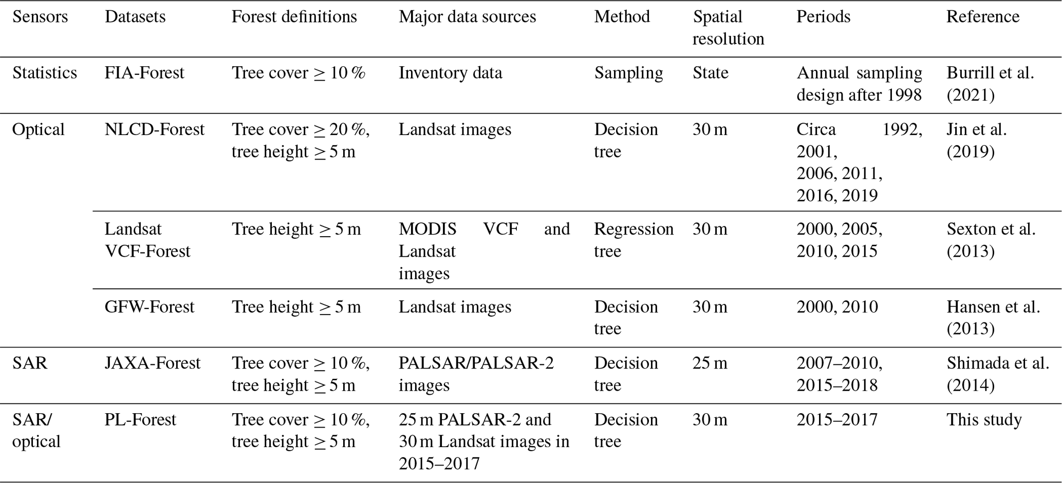
The Landsat images have been used to generate forest or other land cover products at a high spatial resolution (tens of meters) (Chen et al., 2015; Hansen et al., 2013; Jin et al., 2013). The major Landsat-based products for the contiguous United States (CONUS) include the Global Forest Watch (GFW) program of the World Resources Institute (Hansen et al., 2013), the forest cover fraction Vegetation Continuous Field (VCF) product from the Global Land Cover Facility (GLCF) Data Center at the University of Maryland (Sexton et al., 2013), and the National Land Cover Database (NLCD) from the United States Geological Survey (USGS) (Jin et al., 2013). In the USA, FIA and NLCD are the primary databases used by managers, researchers, and policymakers to assess land use and track land management (Hoover et al., 2020; Domke et al., 2021). FIA is a field survey of forest plots and reports information on the status and trends of forests in the USA. A subset of plots is measured every year with revisit intervals of 5 to 10 years, depending on the state (Hoover et al., 2020; Burrill et al., 2021). NLCD provides updated datasets every 3 years or so, which are generated by change detection algorithms for a time period only and have a certain number of commission errors (Jin et al., 2013). Additionally, the annual global forest maps were published by the Japan Aerospace Exploration Agency (JAXA) over the years 2007–2010 and 2015–2018 and were generated using Phased Array type L-band Synthetic Aperture Radar (PALSAR and PALSAR-2) images at 25 and 50 m spatial resolutions (Shimada et al., 2014). The main characteristics of these high-spatial-resolution forest maps covering the CONUS are summarized in Table 1. The wide availability of satellite-based forest and land cover maps makes it easier for stakeholders to access more information than ever before. However, it is still challenging for users to understand the differences between the forest products and clarify their application potential systematically for specific purposes.

Due to the differences in forest definitions, satellite data, in situ training data, and mapping algorithms, the available forest maps still have large discrepancies in forest area estimates (Smith et al., 2018; Qin et al., 2017; Sexton et al., 2016). The optical remote sensing data are affected by cloud cover, cloud shadow, and smoke, which reduce the number of good-quality observations (Reiche et al., 2015). Buildings, rocks, and high-biomass crops often have large PALSAR backscatter coefficients at similar or higher levels of forest (Qin et al., 2017). The combination of the optical and microwave data could take advantage of the optical remote sensors that capture the light and forest canopy interaction, together with L-band microwave sensors that capture the microwave and forest structure (tree trunk and branch) interaction without cloud contamination. One study suggested that the complementarity of optical and synthetic aperture radar (SAR) datasets improved the accuracy of forest maps in comparison to using either an optical dataset or an SAR dataset (Lehmann et al., 2015). For example, misclassification of the Landsat-based forest maps could be caused by replanted areas with small- or medium-sized trees or by regions with vegetation types like highland scrub. However, these regions could be identified correctly by PALSAR data (Lehmann et al., 2015). Improved forest maps have been reported in several studies by using integrated PALSAR and Landsat data in tropical regions (Reiche et al., 2015; Lehmann et al., 2015; Thapa et al., 2014) and PALSAR and MODIS data in monsoon Asia and other regions of the world (Zhang et al., 2019; Qin et al., 2016a). However, the potential of combined PALSAR and Landsat images to improve the annual forest area estimates in the CONUS remains unclear.

In addition to annual forest maps, information on evergreen forests and deciduous forests is important for forest management and conservation. Many studies have shown that the spatial distributions of evergreen and deciduous forests have been changing and will continue to change in the future, driven by multiple stressors involving climate change, forest disturbance, land use change, and invasive species (Soh et al., 2019; Mekonnen et al., 2019; Knott et al., 2019). Accurate distribution information on evergreen and deciduous forest types is also needed to reduce the uncertainty in the carbon budgets (Deb Burman et al., 2021). With the development of Earth observation technology, some efforts have been made to produce forest-type datasets based on multiple spaceborne and/or airborne images (Laurin et al., 2016; Kushwaha, 1990). As an example, for study at the national or continental scale, the NLCD dataset provides the nationwide distribution of deciduous, evergreen, and mixed forests in the USA at 30 m spatial resolution for the years 2001, 2006, 2011, and 2016. The 50 m evergreen and deciduous forest map in 2010 was generated across monsoon Asia using PALSAR and time series MODIS images (Qin et al., 2016a). In addition, time series MODIS images have been reported to improve the estimates of evergreen forests in tropical regions (Qin et al., 2019). As NLCD used multi-temporal Landsat images to identify evergreen and deciduous forests, time series Landsat images could improve the discrimination and classification of evergreen and deciduous forests to support annual analyses in scientific research and policymaking on forest ecosystems. To date, few efforts have been made to produce annual maps of evergreen or deciduous forests over temperate regions, despite their importance.

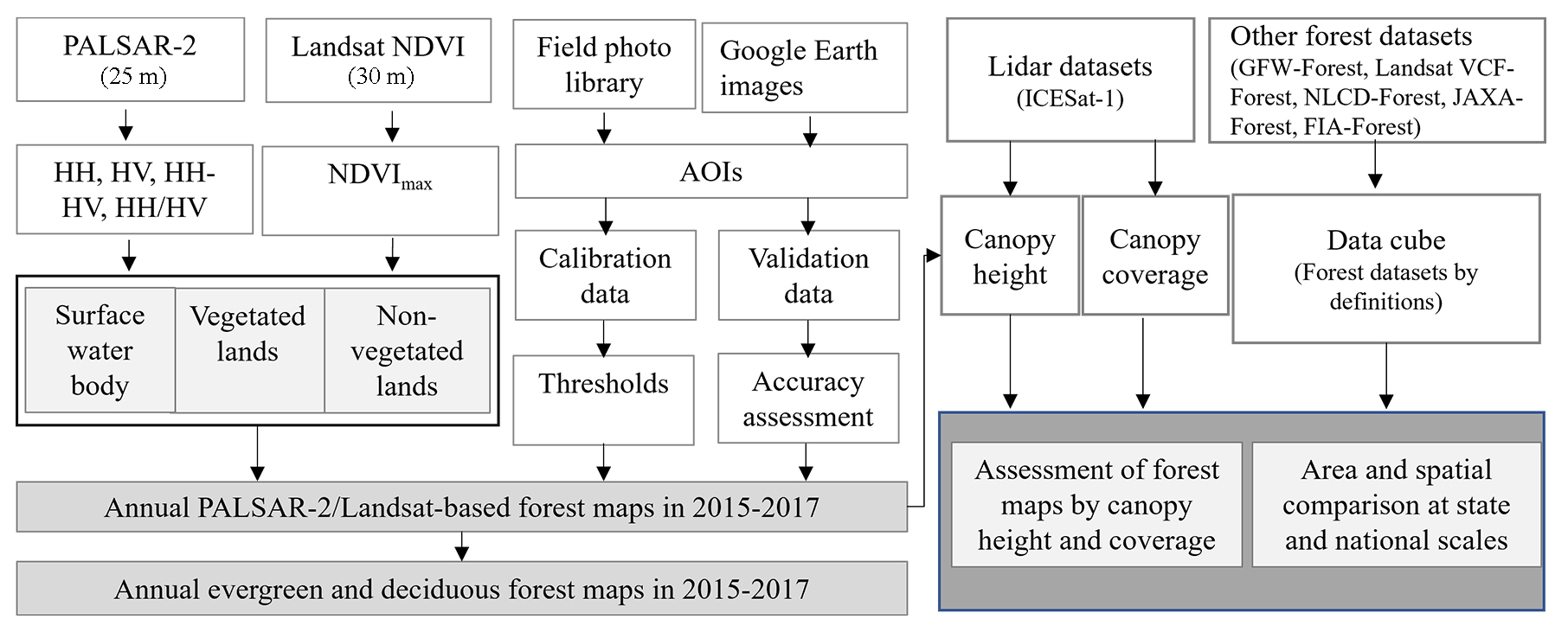
Figure 1 The workflow of this study. It includes three major study sections and the detailed processes of each section in this study. HH, HV, HH − HV, and $\text{HH}/\text{HV}$ denote the horizontal–horizontal (HH) and horizontal–vertical (HV) polarization bands, together with two composite layers of the difference (HH − HV) and the ratio ($\text{HH}/\text{HV}$). AOIs refer to the areas of interest used as calibration and validation samples in this study. GFW-Forest, Landsat VCF-Forest, NLCD-Forest, JAXA-Forest, and FIA-Forest present the forest cover datasets that have been released by the Global Forest Watch program of the World Resources Institute, the Landsat-based forest cover fraction product from the Global Land Cover Facility Data Center at the University of Maryland, the National Land Cover Database from the United States Geological Survey, the Japan Aerospace Exploration Agency forest maps, and the Forest Inventory and Analysis program managed by the U.S. Department of Agriculture Forest Service.

The United Nations Food and Agriculture Organization (FAO) Global Forest Resources Assessment (FRA) has provided essential information for understanding the world's forest resources, management, and uses every 5 years since 1990 by assembling the forest data from individual countries (Keenan et al., 2015). In an effort to improve annual forest maps at a national scale to support the FAO FRA program, this study had three objectives. The first objective was to develop annual forest maps and annual evergreen forest maps in the CONUS by using both PALSAR-2 and Landsat images from 2015 to 2017. The second objective was to assess and compare the resultant PALSAR-2/Landsat-based forest (PL-Forest) maps with the major satellite-based forest cover datasets by using the forest structure data (tree height and tree canopy coverage), which were derived from the observations of the Geoscience Laser Altimetry System (GLAS) on board NASA's Ice, Cloud, and land Elevation Satellite (ICESat-1). This comparison with a large amount of lidar data will help us understand the differences between the forest datasets under the forest definition used by the FAO. The FAO defines forests as lands of more than 0.5 ha with tree cover over 10 % and tree height over 5 m (FAO, 2012). The third objective was to report the PL-Forest maps at two administration levels (state and CONUS) and compare them with the forest area estimates from the FIA of the USDA Forest Service, which are the primary data sources provided by the US government for the FAO Global Forest Resources Assessment. This comparison will help us investigate the ability to combine the PALSAR-2/Landsat approach and the FIA approach to support the Global Forest Resources Assessment at the national scale.

2 Materials and methods

The workflow in Fig. 1 presents the three major study sections and the detailed processes of each section in this study. First, we generated the annual forest maps and annual evergreen and deciduous forest maps at 30 m spatial resolution during 2015–2017 by integrating PALSAR-2 and Landsat time series Normalized Difference Vegetation Index (NDVI) data. Second, we compared the resultant PL-Forest maps with other major satellite-based forest datasets in the study period of 2015–2017. We assessed these forest maps following the FAO's forest definition using the tree height and canopy coverage data from the ICESat-1 lidar-based products. Third, we examined the performance of all the satellite-based forest maps in forest area estimates by comparison with the FIA statistical data at the state and national administration levels.

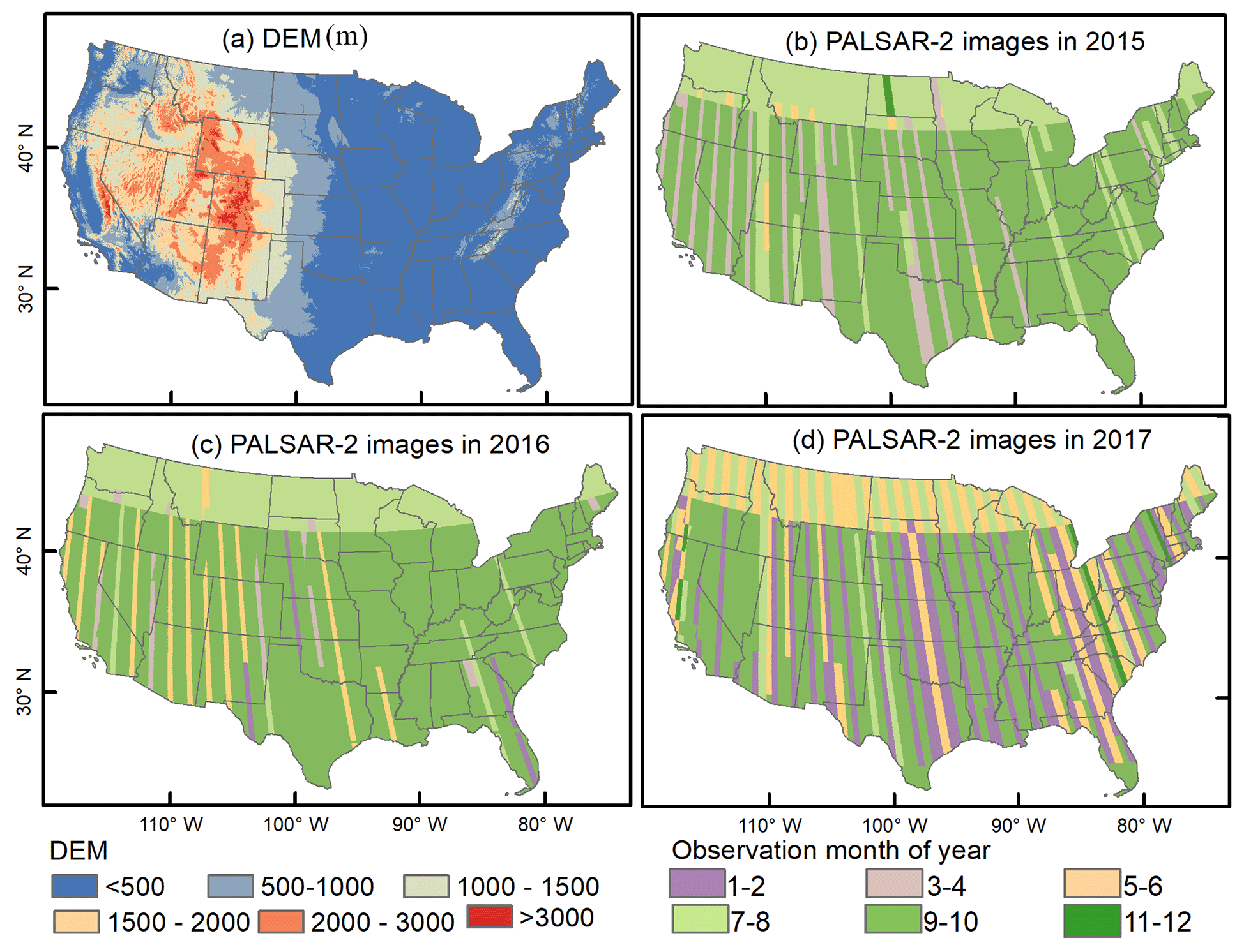
Figure 2 The spatial distributions of (a) the topography of the CONUS using the data from the United States Geological Survey's 3D-Elevation Program 10 m resolution digital elevation model (DEM). (b–d) The acquisition dates of PALSAR-2 images in a year during 2015–2017.

2.1 Study area

Our study area is the CONUS with an area of about 8.08 × 10⁶ km², including the 48 states and Washington, DC. About 50 % of the CONUS land cover change has involved forests since 2001 (Homer et al., 2020). The CONUS has large topographical variation from the eastern USA to the western USA, as shown by the spatial distribution of topography in the CONUS (Fig. 2a).

2.2 PALSAR-2 data in 2015–2017

The annual 25 m ALOS-2 PALSAR-2 mosaic data from 2015 to 2017 were collected on the Google Earth Engine (GEE) platform (https://developers.google.com/earth-engine/datasets/catalog/JAXA_ALOS_PALSAR_YEARLY_SAR, last access: 18 March 2022). The PALSAR-2 horizontal–horizontal (HH) and horizontal–vertical (HV) polarization bands, provided by the Earth Observation Research Center of JAXA, are slope-corrected, radiometrically calibrated, and orthorectified backscatters with a geometric accuracy of around 12 m (Reiche et al., 2018). Figure 2b–d show the acquisition dates of the PALSAR-2 mosaic images over the CONUS, and most images were acquired from May to October. The HH and HV bands were converted from the amplitude values into gamma-naught backscattering coefficients in decibels (γ°) using Eq. (1) (Shimada et al., 2009, 2014; Chen et al., 2018).

$$\begin{array}{}\text{(1)}& \mathit{\gamma }\mathit{°}=\mathrm{10}\times \text{ln}{\text{DN}}^{\mathrm{2}}+\text{CF},\end{array}$$

where γ° is the backscattering coefficient using decibels as the unit, DN is the digital number of amplitude images like the HH or HV bands, and CF is a calibration factor with a value of −83 dB. In addition, two composite layers, i.e., the difference (HH − HV) and the ratio ($\text{HH}/\text{HV}$), were calculated as input data for forest mapping.

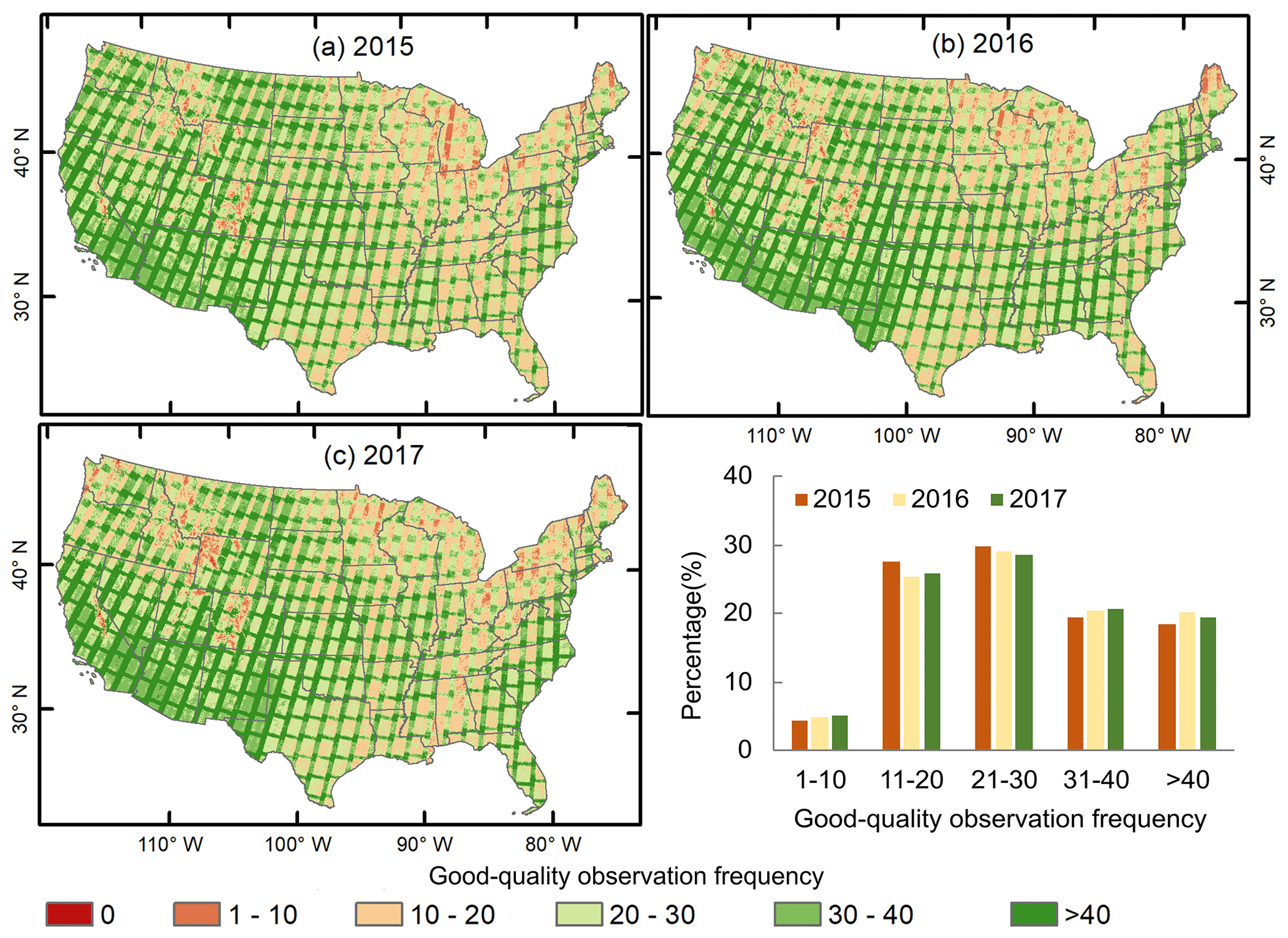
Figure 3 Summary of the good-quality observation frequencies for individual pixels in a year over the CONUS using all Landsat images in a year from 2015 to 2017.

2.3 Landsat data in 2015–2017

We used all the Landsat-7 Enhanced Thematic Mapper (ETM+) and Landsat-8 Operational Land Imager (OLI) surface reflectance (SR) images from 2015 to 2017 to construct a time series image data cube in GEE (https://developers.google.com/earth-engine/datasets/catalog/landsat, last access: 29 September 2024). This dataset provides multi-spectral images at 30 m resolution, and the SR data were derived from top-of-atmosphere (TOA) reflectance by the atmospheric correction codes (Vermote et al., 2016). The bad-quality observations with clouds, cloud shadows, snow or ice, and scan-line-off strips were identified as NODATA following the quality band (pixel_qa). The remaining good-quality observations were used to calculate the vegetation indices NDVI, Enhanced Vegetation Index (EVI), and Land Surface Water Index (LSWI) for each image in the data cube (Eqs. 2–4). Figure 3 shows the spatial distribution of annual total good-quality observation numbers for individual pixels over the CONUS from 2015 to 2017.

$$\begin{array}{}\text{(2)}& {\displaystyle }& {\displaystyle }\text{NDVI}={\displaystyle \frac{{\mathit{\rho }}_{\text{NIR}}-{\mathit{\rho }}_{\text{Red}}}{{\mathit{\rho }}_{\text{NIR}}+{\mathit{\rho }}_{\text{Red}}}},\text{(3)}& {\displaystyle }& {\displaystyle }\text{EVI}=\mathrm{2.5}\times {\displaystyle \frac{{\mathit{\rho }}_{\text{NIR}}-{\mathit{\rho }}_{\text{Red}}}{{\mathit{\rho }}_{\text{NIR}}+\mathrm{6}\times {\mathit{\rho }}_{\text{Red}}-\mathrm{7.5}\times {\mathit{\rho }}_{\text{Blue}}+\mathrm{1}}},\text{(4)}& {\displaystyle }& {\displaystyle }\text{LSWI}={\displaystyle \frac{{\mathit{\rho }}_{\text{NIR}}-{\mathit{\rho }}_{\text{SWIR}}}{{\mathit{\rho }}_{\text{NIR}}+{\mathit{\rho }}_{\text{SWIR}}}},\end{array}$$

where ρ_Blue, ρ_Red, ρ_NIR, and ρ_SWIR are the surface reflectance values of the blue (450–520 nm), red (630–690 nm), near-infrared (760–900 nm), and shortwave-infrared (1550–1750 nm) bands.

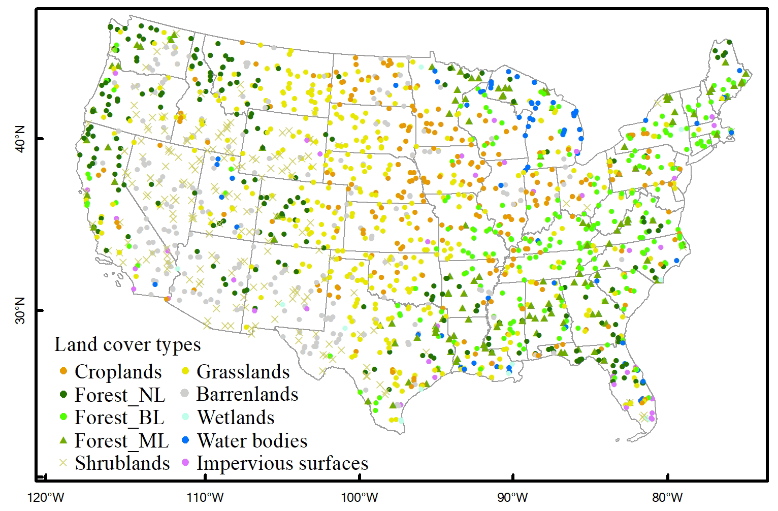
Figure 4 The land cover samples for accuracy assessment in this study. These samples were from the global validation sample set released by the researchers from Tsinghua University, China (http://data.ess.tsinghua.edu.cn/, last access: 20 February 2022) (Gong et al., 2013). They were revised by excluding the samples with land cover change according to the Google Earth images. Forest_NL, Forest_BL, and Forest_ML denote needle-leaved forest, broad-leaved forest, and mixed-leaved forest, respectively.

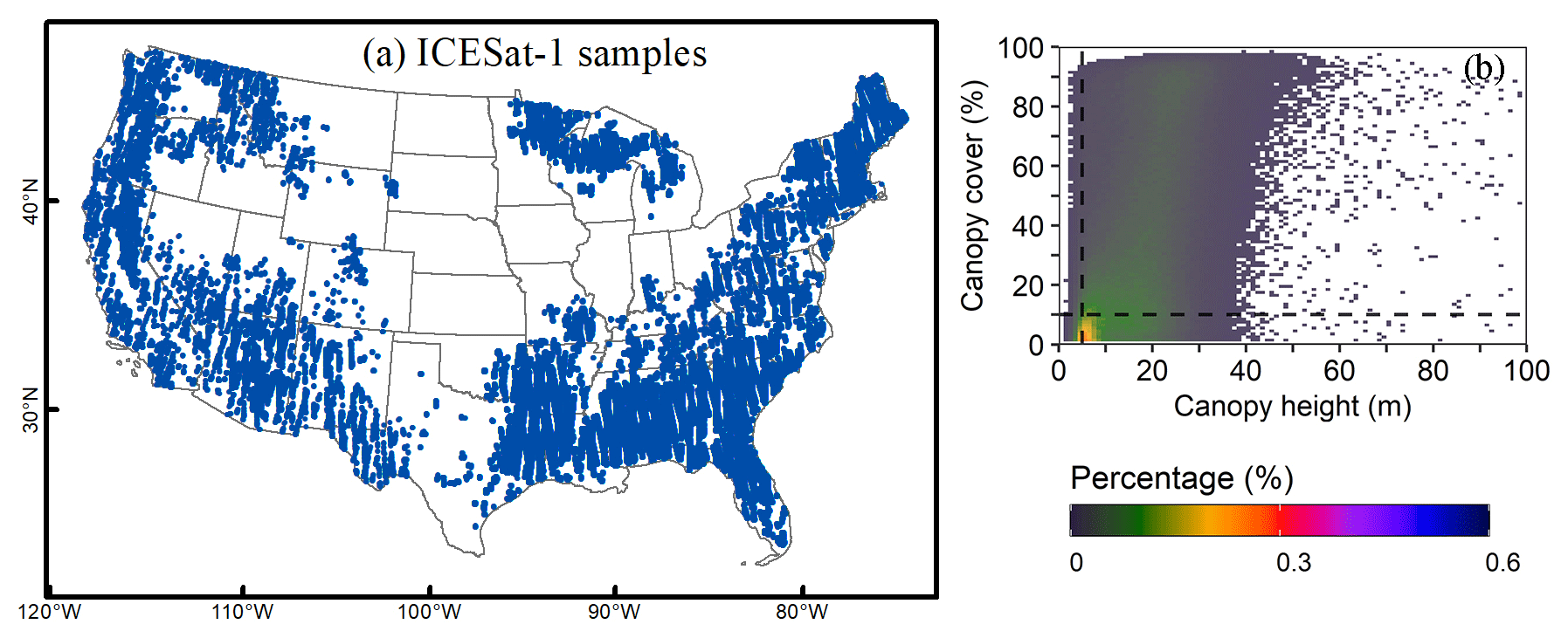
Figure 5 The ICESat samples in the CONUS. (a) Spatial distribution of ICESat-1 samples. (b) Histogram of canopy height (m) and canopy coverage (%) for the ICESat-1 samples.

2.4 Sample data for accuracy assessment of forest maps

The accuracy of the annual PL-Forest maps was assessed based on the global validation sample set released by researchers from Tsinghua University, China (http://data.ess.tsinghua.edu.cn/, last access: 20 February 2022) (Gong et al., 2013). This validation dataset was generated using a random sampling strategy and visual interpretation method for the Finer Resolution Observation and Monitoring-Global Land Cover (FROM-GLC) (Gong et al., 2013). As the validation samples were generated in 2013, in this study we double-checked the land cover types of all the samples by visual interpretation of the Google Earth images during 2015–2017. We deleted those samples with land cover changes (e.g., from forest to non-forest or from non-forest to forest), and thus a total of 652 forest samples were kept for this study. Finally, a total of 1958 points were used for the validation of the resultant forest maps, which include 652 forests, 285 croplands, 431 grasslands, 205 shrublands, 95 water bodies and wetlands, 46 impervious surfaces, and 244 barren lands (Fig. 4).

2.5 Canopy height and canopy coverage data from ICESat lidar

To assess the PL-Forest maps and other forest maps in terms of forest structure traits (canopy height, canopy coverage) that are used in the forest definition of the FAO, we used the ICESat global canopy coverage and height dataset to generate samples of (1) forest canopy height (m) and (2) forest canopy coverage (%). This ICESat dataset was derived based on the observations from GLAS on board NASA's ICESat-1 with a footprint of about 65 m in diameter (Tang et al., 2019). The ICESat mission acquired lidar data over the globe during 2003–2009. The ICESat-based tree canopy cover products provide improved information to characterize biome-level gradients and canopy cover almost without bias at the footprint level (Tang et al., 2019). There are more than 550 000 laser footprints from ICESat-1 over the CONUS (Fig. 5). This is the only available dataset that can be used to assess the structural characteristics of the forests extracted by the forest cover products in the study period of 2015–2017. The image acquisition years differ between the ICESat data (2003–2009) and the PALSAR-2/Landsat data (2015–2017), which may cause small uncertainties in the assessment results. A pixel has three scenarios in terms of forest or not in these two time periods (2003–2009 vs. 2015–2017): (1) as forest in both 2003–2009 and 2015–2017, (2) as forest in 2003–2009 but not in 2015–2017 (forest loss due to deforestation), and (3) as forest in 2015–2017 but not in 2003–2009 (forest gain due to reforestation or afforestation). For those pixels that were forest in both 2003–2009 and 2015–2017 (scenario no. 1), as the canopy height (CH) and canopy coverage (CC) of a forest stand are likely to increase over the years, using CH and CC data in 2003–2009 may underestimate the number of pixels meeting the FAO's forest definition. Those pixels that were forest in only one period of 2003–2009 or 2015–2017 (scenario no. 2 or 3) were not evaluated in the assessment. In addition, the differences in image acquisition years would not affect the results of intercomparison between different forest cover products.

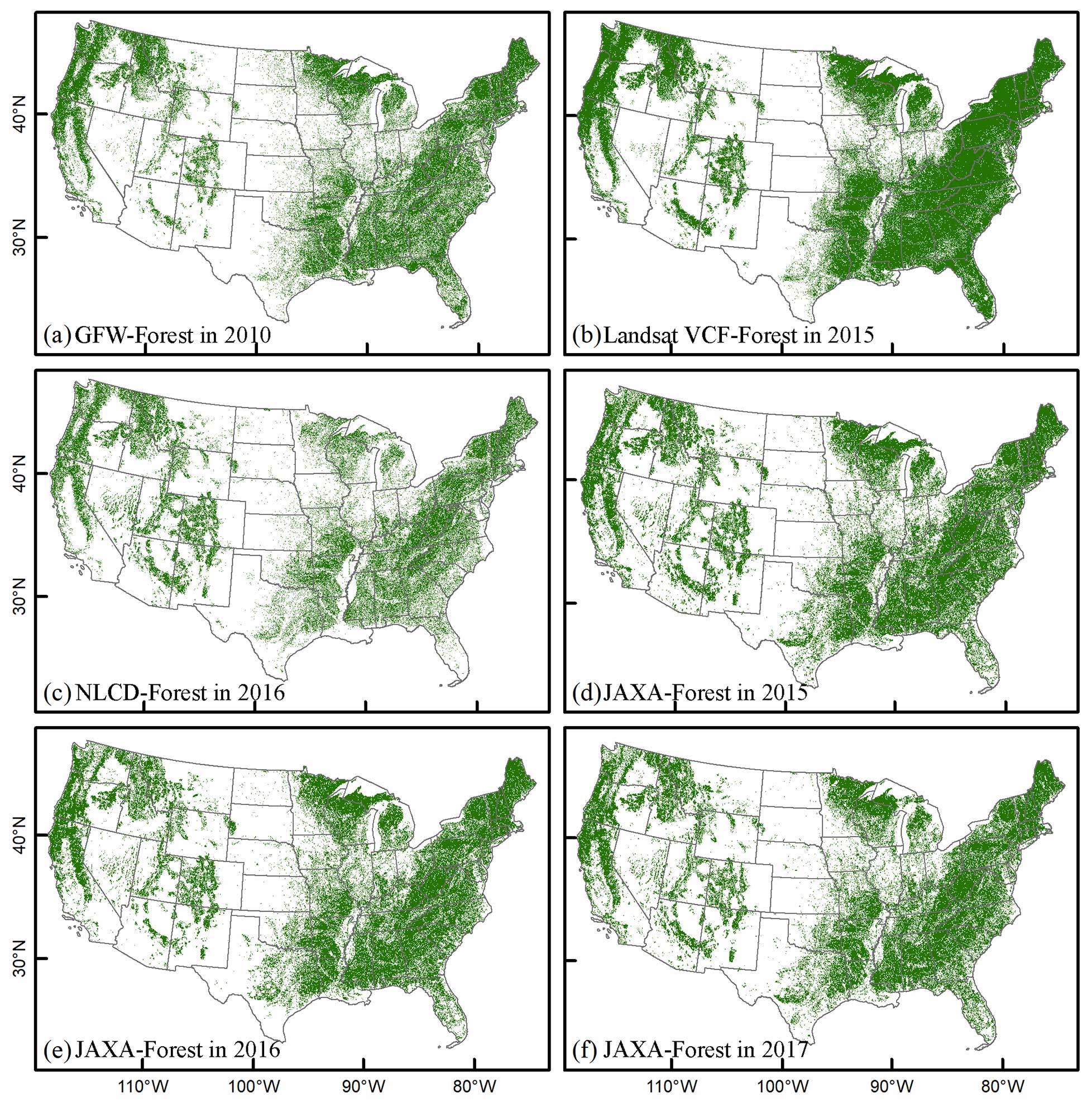
Figure 6 Forest distribution in the CONUS from four forest data products, (a–c) Landsat-based and (d–f) PALSAR-2-based forest products during 2015–2017. GFW-Forest in 2010 presents the forest cover map in 2010 from the Global Forest Watch program of the World Resources Institute. Landsat VCF-Forest in 2015 presents the Landsat-based forest cover fraction product from the Global Land Cover Facility Data Center at the University of Maryland. NLCD-Forest in 2016 presents the forest cover map in 2016 from the National Land Cover Database. JAXA-Forest in 2015–2017 refers to the Japan Aerospace Exploration Agency forest maps from 2015 to 2017.

2.6 Satellite-based forest cover products for intercomparison

We used four forest cover products derived from analyses of satellite images at a high spatial resolution (≤ 30 m) for intercomparison with our PL-Forest maps: the forest product in 2010 from the GFW program of the World Resources Institute, the Landsat-based forest cover fraction product in 2015 from the Global Land Cover Facility Data Center at the University of Maryland (Landsat VCF), the NLCD product in 2016, and the JAXA forest maps in 2015–2017 (JAXA-Forest) (Fig. 6). The GFW tree canopy cover product in 2010 at 30 m resolution was generated by using decision tree algorithms and multi-temporal Landsat images (https://www.glad.umd.edu/dataset/global-2010-tree-cover-30-m, last access: 1 May 2021) (Hansen et al., 2013). The Landsat VCF product in 2015 is a global tree cover percentage dataset and can be downloaded from the Land-Cover and Land-Use Change Program (https://lcluc.umd.edu/metadata/global-30m-landsat-tree-canopy-version-4, last access: 5 May 2021). It is generated by using a regression tree model to rescale the 250 m MODIS VCF tree cover layer to 30 m (Sexton et al., 2013). The Landsat-based NLCD in 2016 provides land cover information at 30 m resolution over the CONUS with an accuracy of 83 % (https://www.mrlc.gov/data/nlcd-2016-land-cover-conus, last access: 9 May 2021) (Homer et al., 2020). This product has three forest types, i.e., deciduous forest, evergreen forest, and mixed forest, which were included in the NLCD-Forest map in this study (Homer et al., 2020). The 25 m annual JAXA-Forest maps from 2015 to 2017 were produced by using the PALSAR-2 mosaic data and a decision tree method and are available at https://www.eorc.jaxa.jp/ALOS/en/palsar_fnf/fnf_index.html, last accessed on 12 May 2021 (Shimada et al., 2014). JAXA-Forest used the FAO's forest definition. So, similarly, for the tree cover products of GFW and Landsat VCF, we selected the pixels with tree canopy coverage greater than 10 % as forests to generate the GFW-Forest and Landsat VCF-Forest maps.

2.7 Forest cover data from an in situ field inventory for intercomparison

The forest area statistical data for the year 2017 at the county scale were also used for comparison analysis (FIA-Forest). This statistical dataset comes from the USDA Forest Service FIA program (https://www.srs.fs.usda.gov/pubs/57903, last access: 10 May 2021) and is widely used in the studies of forests in the CONUS (Domke et al., 2021; Burrill et al., 2021; Hoover et al., 2020). The definition of the forest land condition is that it is larger than 0.4 ha (1.0 acre) in size, is greater than 37 m (120.0 ft) in width, and has at least 10 % canopy cover by live tally of trees of any size at present or in the past (Burrill et al., 2021). Forest land also includes (1) the transition zones, such as areas between forest and non-forest (F/NF) lands that meet the minimal tree canopy cover and forest areas; (2) the strips of roadside, streamside, and shelterbelt trees continuously wider than 37 m (120 ft) and longer than 111 m (363 ft); and (3) the unimproved roads, trails, streams, and clearings in forest areas less than 37 m in width or less than 0.4 ha in size. Forest land does not include tree-covered regions in agricultural production settings like orchards or urban areas like city parks (Burrill et al., 2021). The accuracy standard for forest area in the FIA program is to meet the mandated sampling error of no more than 3 % per 4047 km² (1 million acres) of timberland (Burrill et al., 2021). This is the critical data source provided by the US government for the FAO's Global Forest Resources Assessment and for resource managers and the public to manage and utilize the forest resources of the USA.

2.8 PALSAR-2/Landsat-based annual forest maps in 2015–2017

The advantages of L-band ALSO-2 PALSAR-2 data in penetrating the tree canopy to interact with tree branches and trunks lead to higher-volume backscatter signals from forests than from other land cover types (e.g., grasslands, shrublands, croplands, and water bodies). However, some natural surfaces (e.g., rocky lands) or artificial structures (e.g., buildings) also have high backscatter signals, which could easily cause commission errors in the PALSAR/PALSAR-2-based forest signature analysis (Qin et al., 2017). As these land cover types have low NDVI values, they can be tracked and identified by optical images. According to this knowledge, we developed a two-step forest mapping approach by integration of PALSAR or PALSAR-2 images with optical (e.g., MODIS or Landsat) images in our previous studies, such as in South America (Qin et al., 2017), Asia (Qin et al., 2016a), and Australia (Qin et al., 2021). However, these previous studies were mainly conducted at a lower spatial resolution (e.g., 50 m by PALSAR and MODIS) or attempted for limited spatial scales using PALSAR/PALSAR-2 and Landsat images. The performance of the integrated datasets of PALSAR-2 and Landsat is still unclear for monitoring annual dynamics of forest distributions and forest functional types over temperate regions at a higher spatial resolution of 30 m.

In this study, we used the same workflow (Qin et al., 2016b) to identify and map forest cover in the CONUS. First, we identified forest pixels by using 25 m PALSAR-2 images and the threshold-based algorithm. A pixel is classified as forest if its PALSAR-2 data satisfy −19 ≤ HV ≤ −7.5, 0 ≤ difference ≤ 9.5, and 0.2 ≤ ratio ≤ 0.95. The thresholds for the 25 m PALSAR-2 images had been slightly adjusted from those for the 25 m PALSAR data based on our previous studies on PALSAR and PALSAR-2 signature analyses of F/NF samples (Qin et al., 2016b; Chen et al., 2018). A 5 × 5 window median filter was applied to decrease the potential noise (e.g., salt-and-pepper noise) on the PALSAR-based F/NF maps. These resultant 25 m F/NF maps were resampled to 30 m to match the spatial resolution of Landsat images. Forests usually have a high leaf area index (LAI; larger than 3 m² m⁻²), but rocky lands, barren lands, and built-up surfaces have no or little green vegetation in a year. Due to the LAI and NDVI being closely related to each other, the NDVI value of 0.7 or so usually represents the range of 1–2 m² m⁻² of the LAI depending on the vegetation types, which can be used to identify forest and eliminate the commission errors in the PALSAR/PALSAR-2-based forest maps (Qin et al., 2016b). Here we generated the maximum NDVI layers from all the available Landsat images in each year (January to December) during 2015–2017 and applied the threshold of NDVI_max > 0.7 to the layers to generate the NDVI_max masks and extract the pixels covered by green vegetation. The annual 30 m forest map was produced by overlaying the PALSAR-2-based forest maps and the Landsat-based NDVI_max mask layers.

Post classification, a temporal and logical consistency check was performed on these 3-year F/NF maps to reduce the noise or misclassification in the F/NF sequence (Chen et al., 2018; Qin et al., 2016b). For each pixel in the annual F/NF time series maps from 2015 to 2017, the reasonable forest dynamics were NNN, FNN, NNF, FFF, NFF, and FFN (N denotes non-forest and F denotes forest). The NFN and FNF sequences were considered unreasonable and reprocessed as sequences of NNN and FFF, respectively. This 3-year consistency check during 2015–2017 gives higher confidence to the annual forest map in 2016, and we will use it for intercomparison and forest area estimates at the county, state, and CONUS scales. Thus, the annual PL-Forest maps were generated based on the PALSAR-2/Landsat images in this study.

2.9 PALSAR-2/Landsat-based annual evergreen forest maps in 2015–2017

Evergreen trees have green leaves all year round, but deciduous trees usually shed their leaves in winter or in dry seasons. These leaf phenological profiles can be captured by the satellite-based vegetation indices (i.e., NDVI, EVI, and LSWI) to distinguish between evergreen and deciduous forests (Qin et al., 2016a; Prabakaran et al., 2013). Based on the characteristics of forest canopy phenology and vegetation indices, we have developed a simple and robust algorithm to map evergreen forests by analyzing the time series water-related index (LSWI) and greenness-related indices (EVI and NDVI). The green leaves of evergreen forests have positive LSWI values all year round and relatively high EVI values in winter and/or dry seasons, and thus the seasonal profile analysis of LSWI and EVI was used to identify evergreen forests (Qin et al., 2016a). The same approach was used to generate the annual maps of evergreen vegetation using the criteria of pixels with (1) LSWI ≥ 0 for all good observation images in a year and (2) a minimum EVI (EVI_min) of no less than 0.2 identified as evergreen cover. This rule can be characterized by the frequency of LSWI ≥ 0 (FQ_LSWI≥0) for all good observations in a year and EVI_min using the decision thresholds (FQ_LSWI≥0 = 100 % and EVI_min ≥ 0.2). Here, FQ_LSWI≥0 was calculated using the number of observations with LSWI ≥ 0 (N_LSWI≥0) over the number of good-quality observations (N_GOBs) in a year for individual pixels (Eq. 5). Finally, we overlaid our annual 30 m PL-Forest map with the evergreen vegetation layer to identify the annual evergreen forests (called PL-Evergreen Forest maps in this study). Thus, evergreen forests refer to forest land with green leaves throughout the year, with a tree canopy height greater than 5 m and a tree canopy cover larger than 10 %. In this study, both the forests and evergreen forests include natural and artificial forests that meet the requirements (Qin et al., 2024). Meanwhile, as the evergreen forests were extracted based on the greenness signature observed by the satellite images, this map includes both needle-leaved and broad-leaved evergreen forests that meet the requirements.

$$\begin{array}{}\text{(5)}& {\mathrm{FQ}}_{\mathrm{LSWI}\ge \mathrm{0}}={\displaystyle \frac{N_{\mathrm{LSWI}\ge \mathrm{0}}}{N_{\mathrm{GOBs}}}}\times \mathrm{100}\end{array}$$

2.10 Validation

The resultant PL-Forest maps in 2015–2017 were validated using the samples generated by the researchers from Tsinghua University, China (Gong et al., 2013) (Fig. 4). We overlaid the samples and the resultant PL-Forest maps to calculate the confusion matrix and assess the user, producer, and overall accuracies.

2.11 Cross-comparison between forest-related products

We selected the five forest cover data products at 25 or 30 m spatial resolution to perform the intercomparison analysis at three spatial scales: (1) assessment of forest or non-forest identification with forest height and canopy coverage data at the pixel scale, (2) forest area estimates at the state scale, and (3) forest area estimates at the CONUS scale.

Firstly, to understand the differences in terms of forest structure measurements in the PALSAR-2-based, Landsat-based, and PL-Forest maps, we overlaid the ICESat-1 samples and individual forest products to identify those forest pixels that geographically correspond to the ICESat-1 samples and gather their information on the attributes of forest canopy height and canopy coverage. In this process, all the forest products were resampled into 70 m to match the footprint size of ICESat-1. Then, the distributions of the forest pixels were analyzed with the canopy height and canopy coverage for individual forest maps by using 1-D histogram and 2-D histogram graphs.

Secondly, we compared our PL-Forest-based forest maps with the five selected forest datasets in terms of forest areas at the state scale. All the forest maps were reprojected into equal-area projection before the forest areas were calculated from individual maps. The linear regression approach was used to show the relationships between these forest datasets for forest areas at the state level.

Thirdly, the forest area estimates at the national level were directly compared amongst themselves. Based on the reprojected forest maps, the forest areas were calculated in the CONUS region from each individual map. The results for the forest area of the CONUS were compared amongst themselves.

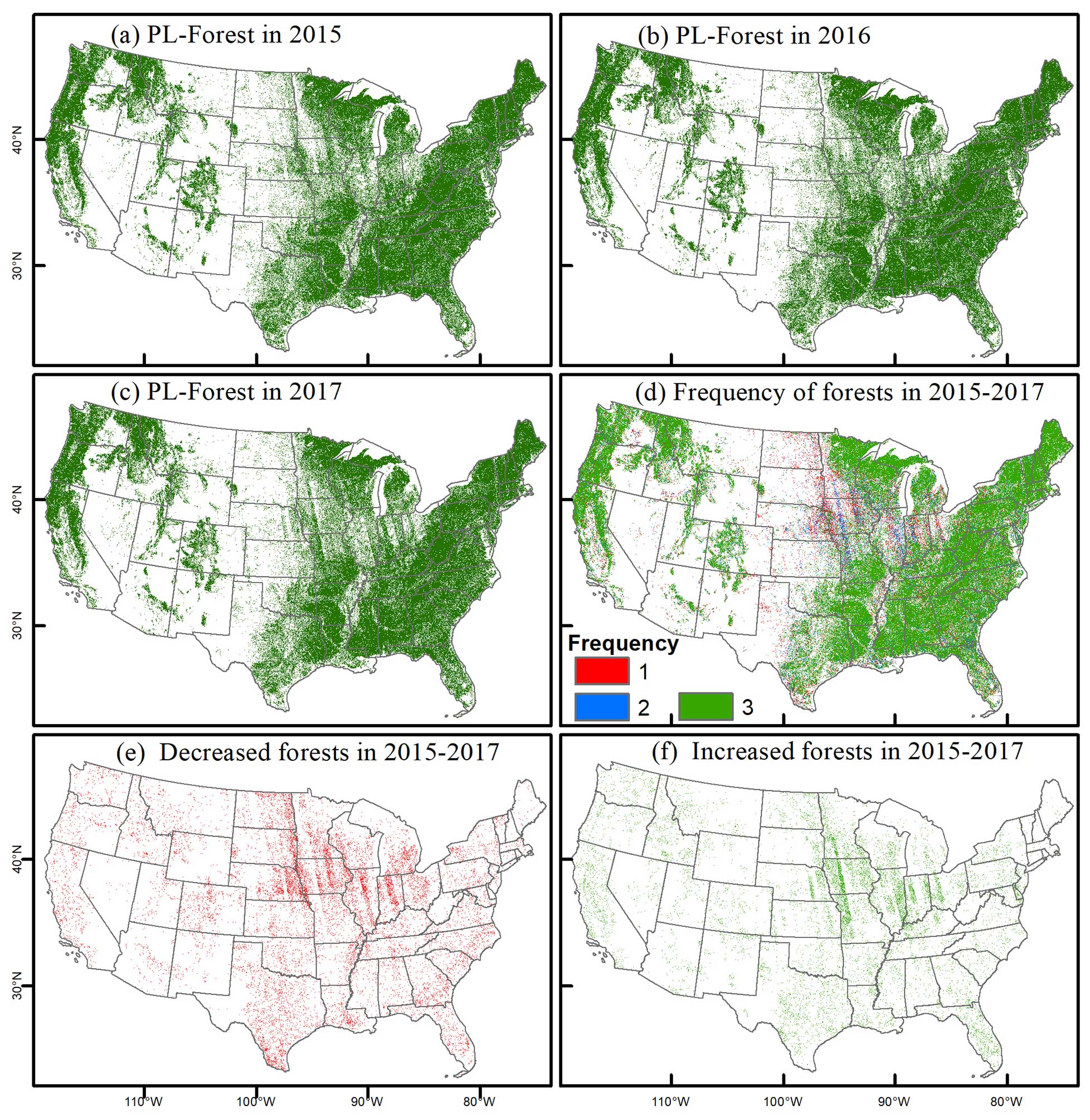
Figure 7 Annual forest maps in 2015–2017 based on PALSAR-2 and Landsat images (PL-Forest): (a) PL-Forest in 2015, (b) PL-Forest in 2016, and (c) PL-Forest in 2017. (d) The forest frequency map was generated based on the PL-Forest maps in 2015–2017. The colors red, blue, and green denote the numbers of a specific pixel classified as forest in the annual PL-Forest maps from 2015 to 2017. (e) The decreased forest in 2015–2017. (f) The increased forest in 2015–2017.

3 Results

3.1 Annual PALSAR-2/Landsat-based forest and evergreen forest maps in 2015–2017

The PL-Forest maps show the annual forest distribution in the CONUS from 2015 to 2017 (Fig. 7a–c). At the pixel level, we calculated the frequency of individual pixels covered by forest in 2015–2017 (Fig. 7d): 79 % of the forest pixels have consistent forest cover from 2015 to 2017 with a frequency of 3, which is much larger than the proportions of forest pixels with 1 year (11 %) or 2 years (10 %) of forest cover. The forest dynamics from 2015 to 2017 are shown in Fig. 7e and f. They suggest that more forest decreases than increases, especially in the central regions.

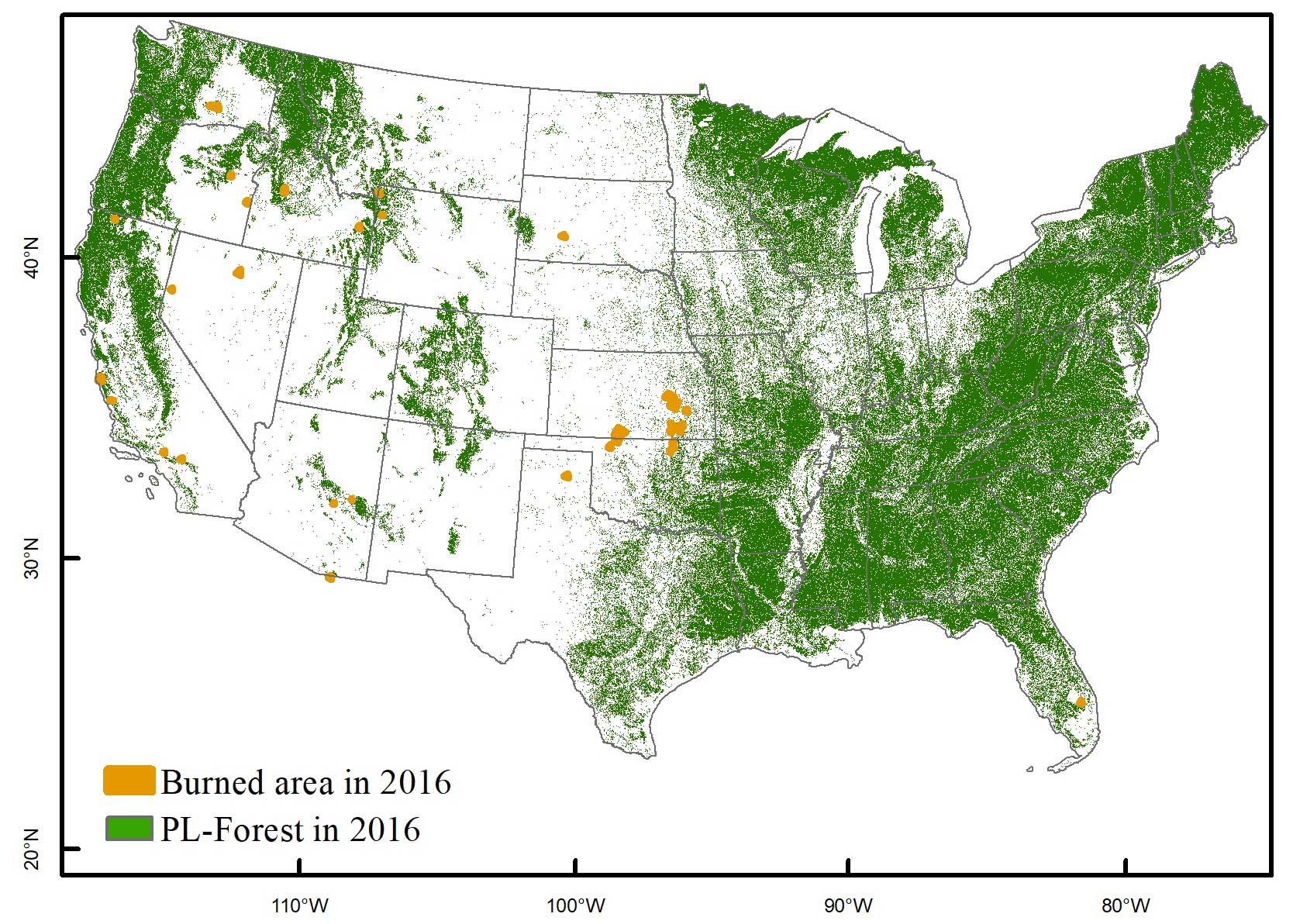
Figure 8 Distribution of burned areas overlaid with the PALSAR-2/Landsat-based forest (PL-Forest) map in 2016. The burned area in 2016 was generated from the MODIS Burned Area Monthly Global 500 m products (MCD64A1.061). If a pixel was burned in any month, it was considered a burned area in 2016.

Table 2 Accuracy assessment of annual PALSAR-2/Landsat-based forest maps in 2015–2017 (PL-Forest) based on the validation samples (Fig. 4). The user (UA), producer (PA), and overall (OA) accuracies are shown.

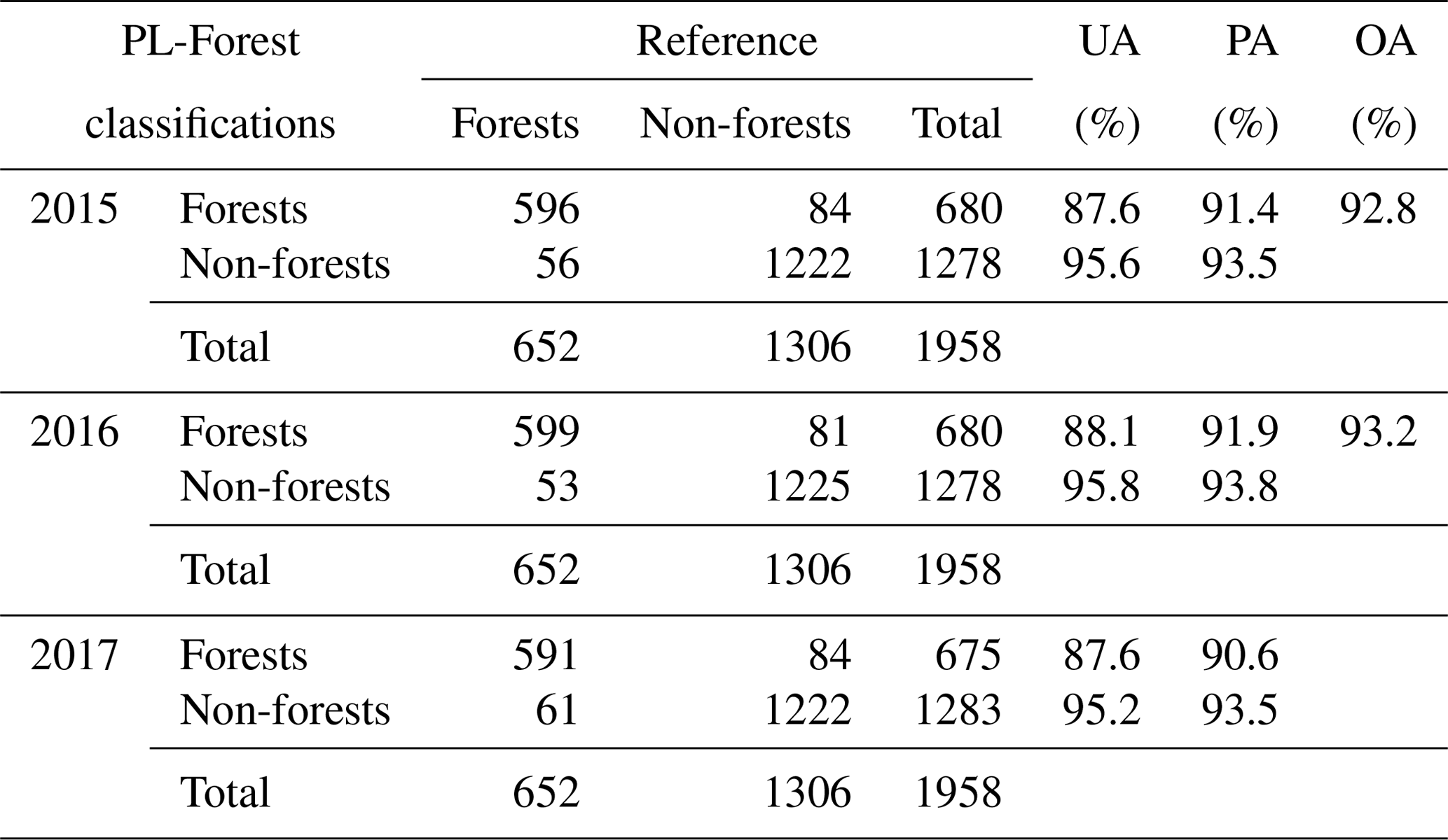
Table 3 Accuracy assessment of the PALSAR-2/Landsat-based forest map in 2016 (PL-Forest) with different elevations (m a.s.l.) based on the validation samples (Fig. 4). The UA, PA, and OA accuracies are shown.

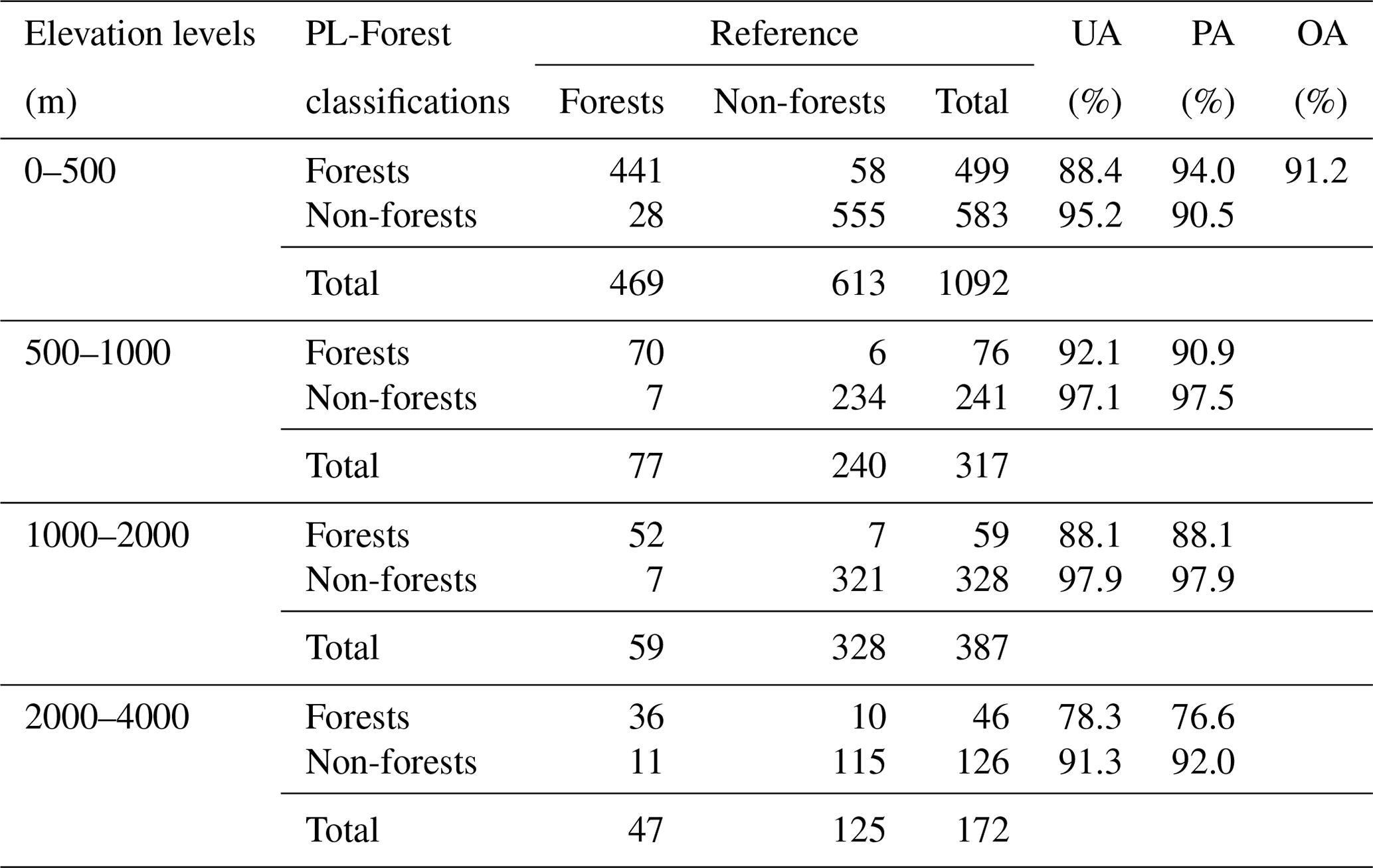
Based on the validation samples (Fig. 4), the accuracies of the PL-Forest maps were high and varied slightly for the years 2015 to 2017: the overall accuracies were ∼ 93 %, the user accuracies were 87.6 % to 95.8 %, and the producer accuracies were 90.6 % to 91.9 % (Table 2). The forest map in 2016 had a slightly higher accuracy than in 2015 and 2017, which was expected because the temporal and logical consistency check was implemented on the resultant map of 2016 to reduce the noise or misclassification in the F/NF sequence of 2015 to 2017 (see Sect. 2.7). The accuracies were comparable to the PALSAR-based forest maps that reported overall accuracies exceeding 91 % (Shimada et al., 2014). In detail, the accuracies of the PL-Forest maps in 2016 were estimated at different altitudes of 0–500, 500–1000, 1000–2000, and 2000–4000 m (Table 3). The results showed that the areas with altitudes lower than 2000 m have user and producer accuracies greater than 88 % and overall accuracies greater than 91 %. The areas with altitudes higher than 2000 m have slightly lower user (78.3 %), producer (76.6 %), and overall (87.8 %) accuracies. Additionally, we examined the potential of PL-Forest in 2016 to exclude the impacts of the burned area by overlaying a MODIS burned-area product and the forest map (Fig. 8). The results showed that there were 6 845 692 pixels covered by burned areas, and 713 003 pixels were identified as forests in the resultant PL-Forest map in 2016 with a proportion of about 10.4 %. However, this number may not accurately represent the commission error, as the burned forest may not be fully dead and could regrow again.

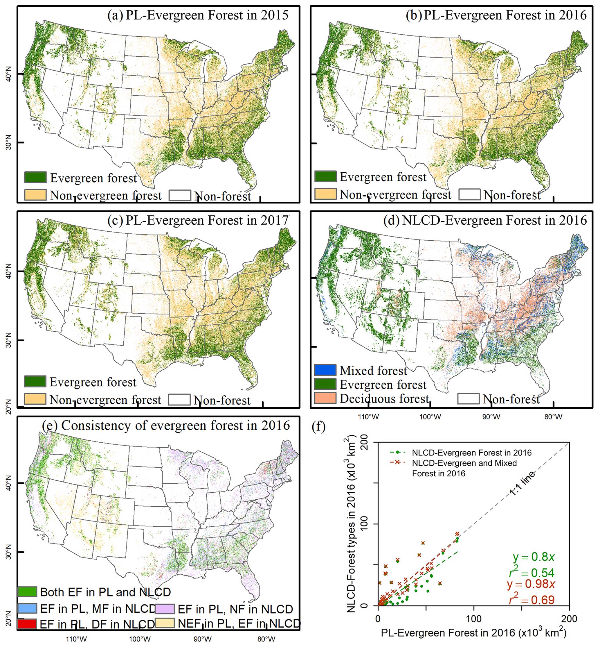
Figure 9 Spatial distributions of evergreen forests in the CONUS. (a–c) Annual evergreen and non-evergreen forest maps generated from the PALSAR-2/Landsat (PL) images in 2015–2017. (d) The forest-type map from the National Land Cover Database (NLCD) in the 2016 dataset. Panel (e) shows the consistency between PL-Evergreen Forest in 2016 and NLCD-Evergreen Forest in 2016. The abbreviations are Evergreen Forest (EF), PL-Evergreen Forest in 2016 (PL), Mixed Forest (MF), Non-Forest (NF), Deciduous Forest (DF), and Non-Evergreen Forest (NEF). Panel (f) shows the comparison between PL-Evergreen Forest, NLCD-Evergreen Forest, NLCD-Evergreen, and Mixed Forest in 2016 at the state scale using linear regression analysis.

Based on the PL-Forest maps, we further generated annual PL-Evergreen Forest maps in the CONUS during 2015–2017 (Fig. 9a–c). These PL-Evergreen Forest maps have spatial patterns that are similar to the evergreen forests in the NLCD dataset in 2016 (Fig. 9d). Evergreen forests show obvious regional characteristics and are mainly distributed in the western, southeastern, and northeastern regions of the CONUS. The evergreen forest area estimated from the PL-Evergreen Forest map in 2016 was 1.08 × 10⁶ km², which is higher than that of the evergreen forests of 0.92 × 10⁶ km² but lower than the total area of evergreen forests and mixed forests of 1.22 × 10⁶ km² from NLCD in 2016 (Fig. 9a–d). The spatial comparison between these two products was carried out at the pixel scale (Fig. 9e). The noticeable discrepancies were in the southwestern regions (e.g., Nevada, Utah, or Arizona), southern Florida, and some regions in the northeastern CONUS. In the southwestern regions, the differences were mainly from the detection of evergreen and non-evergreen forests between these two products. For the eastern regions (e.g., southern Florida and the New England states), the differences between these two products were mostly caused by the detection of forests, as most of the evergreen forest pixels on the PL-Evergreen Forest map were shown as non-forest on the NLCD map (Fig. 9e). At the state scale, the PL-Evergreen Forest map in 2016 had a good linear relationship with the evergreen forests of NLCD in 2016, with a slope of 0.8 and R² of 0.54 (Fig. 9f). A stronger relationship was found between the evergreen forest areas from the PL-Evergreen Forest map in 2016 and the sum of evergreen forests and mixed forests from NLCD in 2016 at the state scale, with a slope of 0.98 and R² of 0.69 (Fig. 9f). One possible explanation could be that the mixed forests in NLCD include evergreen species (Selkowitz and Stehman, 2011). However, this cannot be estimated quantitatively because it is uncertain about the forest types and proportions within the mixed forest pixels (Tran et al., 2016).

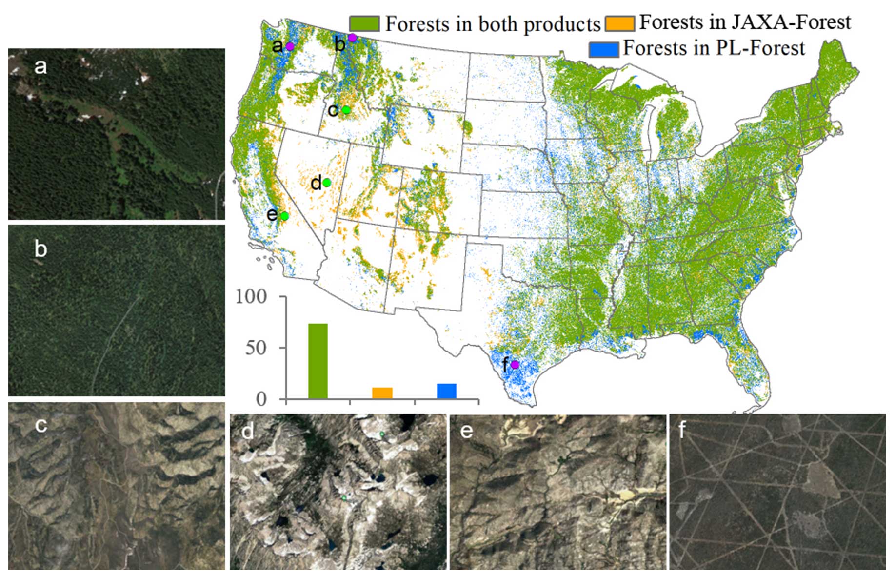
Figure 10 A comparison between the PALSAR-2/Landsat-based forest (PL-Forest) map in 2016 and the Japan Aerospace Exploration Agency forest (JAXA-Forest) map in 2016 at the pixel scale. Six random areas denoted as “a” to “f” were selected from the disagreement regions, which were used to show the zoomed-in landscapes from the Google Earth high-resolution images. The images were acquired from Google Earth Pro (©Google Earth Pro 2020).

3.2 A comparison of five satellite-based forest maps at the pixel scale

At the pixel scale, we compared PL-Forest and JAXA-Forest in 2016 in terms of forest area identification (Fig. 10). These two products have about 75 % of their pixels in agreement, 11 % of them only being identified by JAXA-Forest and 14 % of them only being identified by PL-Forest. Comparison through zoomed-in random samples showed that some pixels with obvious backgrounds of barren lands or rocks have been classified as forests in JAXA-Forest, which were excluded in PL-Forest. However, over the regions with dense tree cover, there are more omission errors in the JAXA-Forest map than were identified in the PL-Forest map (Fig. 10).

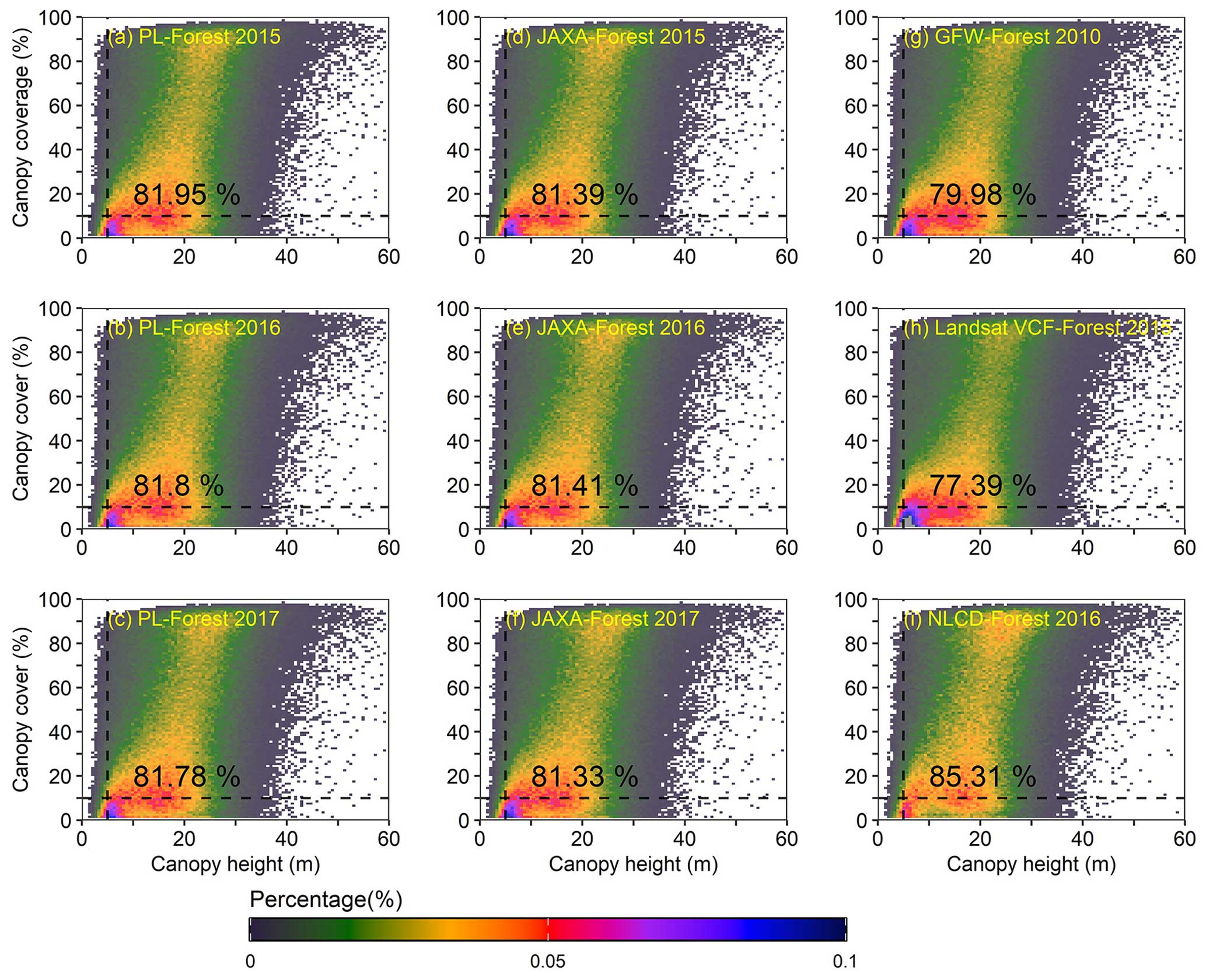
Figure 11 The frequency distributions of the forest pixels with tree canopy height (CH) and canopy cover (CC) features. The forest pixels were from the five satellite-based forest products. The CH and CC data were extracted from the ICESat-1 observations. PL-Forest is the PALSAR-2/Landsat-based forest map generated in this study. JAXA-Forest is the Japan Aerospace Exploration Agency forest map from 2015 to 2017. GFW-Forest 2010 is the forest map in 2010 from the Global Forest Watch program of the World Resources Institute. Landsat VCF-Forest 2015 is the Landsat-based forest cover fraction product in 2015 from the Global Land Cover Facility Data Center at the University of Maryland. NLCD-Forest 2016 refers to the forest map from the National Land Cover Database in 2016 provided by the United States Geological Survey.

We further compared the five studied satellite-based forest data products in terms of their forest definitions of canopy (tree) height and canopy coverage. The frequency distributions of the forest pixels with CH and CC were extracted from different forest products using ICESat-1 observations (Fig. 11). The comparison result showed that the proportion of forest pixels with CH more than 5 m and CC more than 10 % was 85 % for NLCD-Forest in 2016, ∼ 82 % for the PL-Forest maps, 81 % for the JAXA-Forest maps, 80 % for the GFW-Forest maps in 2010 (79.98 %), and 77 % for the Landsat VCF-Forest maps in 2015.

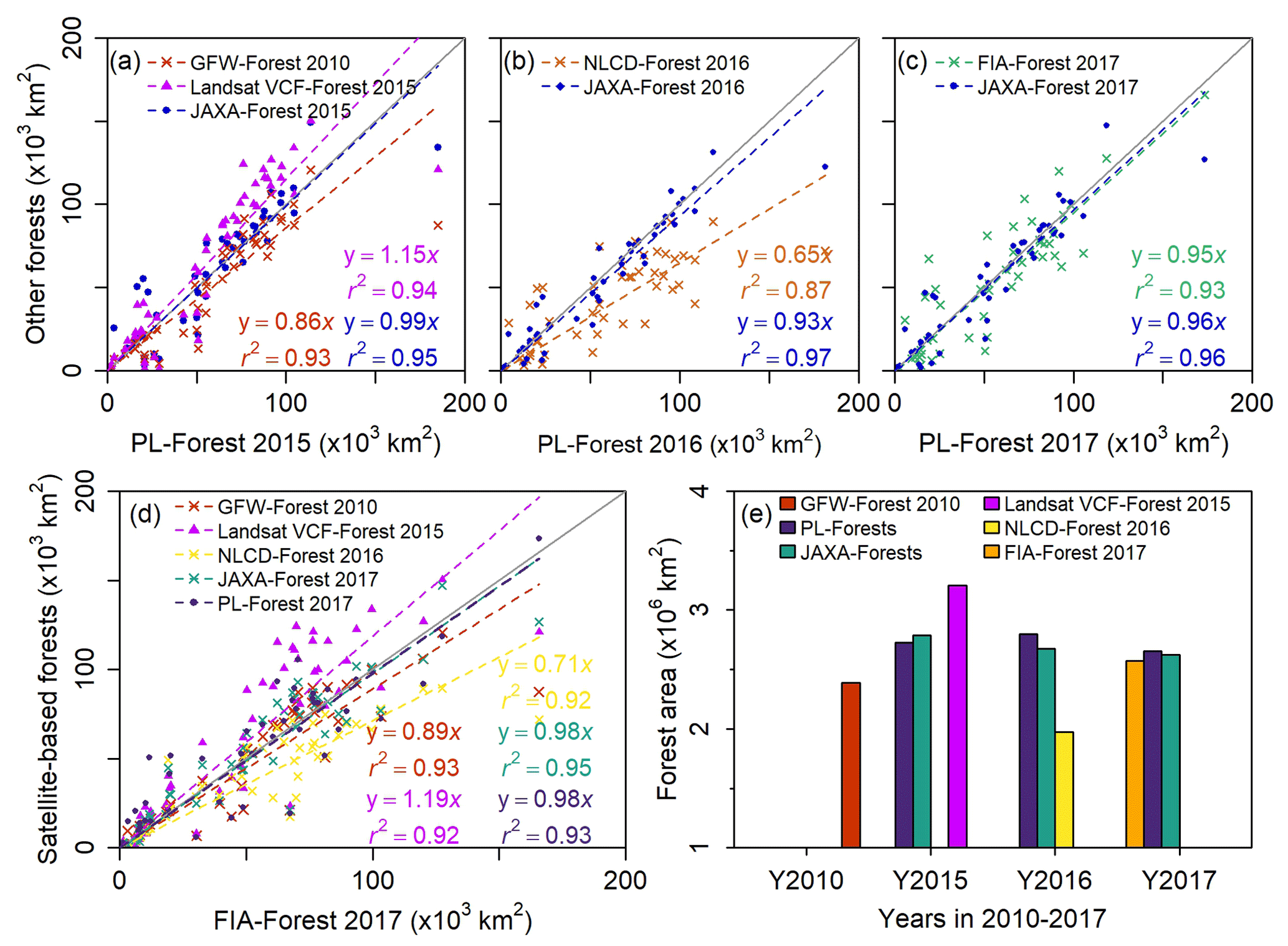
Figure 12 Comparisons of forest area estimates between satellite-based forest products and FIA statistics at the state and national scales. PL-Forest is the annual PALSAR-2/Landsat-based forest map in 2015–2017 generated in this study. JAXA-Forest maps are the Japan Aerospace Exploration Agency forest maps from 2015 to 2017. GFW-Forest 2010 is the forest map in 2010 from the Global Forest Watch program of the World Resources Institute. Landsat VCF-Forest 2015 is the Landsat-based forest cover fraction product in 2015 from the Global Land Cover Facility Data Center at the University of Maryland. NLCD-Forest 2016 refers to the forest map from the National Land Cover Database in 2016 provided by the United States Geological Survey. FIA-Forest 2017 presents the forest cover datasets from the Forest Inventory and Analysis program in 2017.

3.3 A comparison of forest area estimates from six forest datasets at the state and CONUS scales

The forest areas were estimated at the state and CONUS scales from the six forest datasets, including five satellite-based forest maps in 2010–2017 and FIA statistical data in 2017 (Fig. 12). At the state scale, the PL-Forest maps have good linear relationships with other satellite-based datasets for each year during 2015 to 2017, with the slope ranging from 0.65 to 1.15 and R² from 0.87 to 0.96 (Fig. 12a–c). In terms of forest area estimates at the state scale, the PL-Forest and JAXA-Forest maps showed higher agreements with the FIA-Forest dataset than do GFW-Forest 2010, Landsat VCF-Forest 2015, and NLCD-Forest 2016 (Fig. 12d). The forest area estimates from Landsat VCF-Forest 2015 were higher than the FIA-Forest area estimates (slope of 1.19), while the forest area estimates from GFW-Forest 2010 and NLCD-Forest 2016 were lower than the FIA-Forest area estimates (slopes of 0.89 and 0.71) (Fig. 12d). The forest area estimates from the PL-Forest and JAXA-Forest maps were very close to the numbers from FIA-Forest (slope of 0.98).

At the CONUS scale, the forest area estimates from the PL-Forest maps for the years 2015 to 2017 were 2.73 × 10⁶, 2.79 × 10⁶, and 2.66 × 10⁶ km², respectively, and were similar to the areas of the JAXA-Forest maps of 2.79 × 10⁶, 2.68 × 10⁶, and 2.62 × 10⁶ km² (Fig. 12e). The FIA-Forest dataset reported a forest area of 2.57 × 10⁶ km² in 2017, which was very close to the value of 2.66 × 10⁶ km² from the PL-Forest map in 2017 (a difference of 3.5 %).

3.4 Discussion

3.5 Improved annual forest maps at high spatial resolution

To improve the accuracy of the forest cover maps, several efforts have examined the likely factors causing the uncertainties of the resultant products (Sexton et al., 2016; Sexton et al., 2013; Tchuenté et al., 2011; Qin et al., 2016a). These factors include (1) the diverse forest cover definitions, (2) input image datasets, (3) training samples, and (4) algorithms (Qin et al., 2021; Tchuenté et al., 2011). For example, the forest definitions use different criteria for tree coverage (from 10 % to 60 %), tree height (from 2 m to 5 m), and parcel size (Qin et al., 2016a; Sexton et al., 2016). To reduce the uncertainty in the forest maps from the perspective of forest definition, a solution was proposed by Sexton et al. (2016) to focus on the measurable ecological characteristics of tree cover, canopy height, biomass, and composition of vegetation. This study provided a comprehensive assessment through intercomparison with the widely used forest products using the FAO's forest definition and the lidar-based forest structural data (CC and CH) as references. The comparison between forest datasets suggested that PL-Forest had a slightly higher percentage of pixels than JAXA-Forest, GFW-Forest 2010, and Landsat VCF-Forest 2015, in line with the FAO's forest criteria of tree heights greater than 5 m and/or canopy covers larger than 10 %. By this criterion, NLCD-Forest 2016 had the highest pixel proportion, but this dataset used a tree canopy cover larger than 20 % as the forest threshold that resulted in the lowest forest area estimate (Fig. 12e). The comparison results based on the PL-Forest maps agree well with our recent study on forest mapping in Australia, which demonstrated that the PALSAR/MODIS forest maps had more forest pixels satisfied with the FAO's forest definition than the GFW-Forest and JAXA-Forest maps (Qin et al., 2021).

Forest cover products have been generated based on optical images (e.g., MODIS or Landsat), microwave images (e.g., PALSAR or PALSAR-2), or integration of microwave and optical images (e.g., PALSAR/MODIS or PALSAR/Landsat). For the forest area estimates, under a consistent tree canopy cover definition (10 %), the PL-Forest products had results close to the JAXA-Forest (i.e., PALSAR-2-based forest) maps for the years 2015 to 2017 at both the state and national scales (Fig. 12). The forest area estimates in 2017 from the PL-Forest dataset were very close to the result from the FIA-Forest dataset, which indicates that the PL-Forest dataset is more accurate than the forest area estimates from the other optical satellite-based forest products (Fig. 12e). One of the reasons for the improved accuracy could be the utilization of PALSAR-2 images, which (1) are less affected by atmospheric conditions, clouds, and cloud shadows than optical data and (2) have stronger penetration capability into forest canopy with more sensitivity to forest structure (Shimada et al., 2014). Our previous studies also showed similar forest area estimates from the PALSAR/MODIS or PALSAR/Landsat forest products and the JAXA-Forest maps in several regions like monsoon Asia (Qin et al., 2016a) and South America (Qin et al., 2017). For example, in South America, forest area estimates from the 30 m GFW-Forest 2010 dataset were higher than those from the 50 m PALSAR/MODIS forest products (Qin et al., 2017). In addition, GFW-Forest in 2010 and Landsat VCF-Forest in 2015 present the forest cover in the CONUS in the years 2010 and 2015. The inconsistent time with FIA-Forest in 2017 may contribute to some discrepancies between them that would be difficult to quantify.

The results mentioned above also suggested that PL-Forest had a slightly better performance than the other four forest products, according to the potential of forest tree height and tree canopy cover monitoring, and forest area estimates. This result corroborates the previous claims for integrating microwave and optical images to improve forest cover maps (Reiche et al., 2015; Lehmann et al., 2015; Thapa et al., 2014). These forest mapping approaches take advantage of (1) the sensitivity of microwave signals to forest structures without weather interference (Næsset et al., 2016; Qin et al., 2016a) and (2) the optical signals to reduce the number of ground objects with backscatter values similar to those of forests, such as rocky lands and buildings (Reiche et al., 2015; Lehmann et al., 2015) (Fig. 10). The integration of PALSAR and MODIS images has been demonstrated to generate improved forest maps in tropical, temperate, and boreal forests with overall accuracies above 90 % (Zhang et al., 2019; Qin et al., 2017, 2016a). This study produced forest maps with an overall accuracy of about 93 %, which corroborated the potential of combining PALSAR-2 and Landsat observations to monitor the annual dynamics of forest distributions and functional types at a high spatial resolution for national or larger scales across temperate regions. It also suggested the potential of integrating FIA data and PL-Forest products to support the FAO's Global Forest Resources Assessment at the national scale.

However, there could be some uncertainties and limitations when applying this approach. Firstly, although the thresholds of PALSAR-2 signatures for extracting forests were trained by numerous samples, they could have been impacted by forest composition and structures (Chen et al., 2018). Thus, a careful study of the thresholds using samples of specific areas could provide more information that affects the accuracy and uncertainty of the forest maps when applying the algorithms to other regions. In addition, due to the PALSAR data not being available during 2011–2014, we cannot apply this PALSAR/optical data approach in these 4 years. PALSAR data are available for 2007–2010, and thus a combination of PALSAR (2007–2010), PALSAR-2 (2015 to present), and optical images would develop forest maps to monitor forest changes since 2007 (Zhang et al., 2019).

3.6 Evergreen forest mapping algorithms

Evergreen forests show different functional traits from deciduous forests, such as water use efficiency (Soh et al., 2019) and high ecosystem stability in carbon sinks in extreme climates (Huang and Xia, 2019). Driven by climate change and diverse human activities, the expansion of evergreen forests has been reported in many regions all over the world (Twidwell et al., 2016; Saintilan and Rogers, 2015). Various mapping algorithms have been developed to identify evergreen and non-evergreen forests, which could provide accurate information on evergreen forests for science and policy users (Qin et al., 2016a). These evergreen forest mapping algorithms can be grouped as (1) NDVI-based and (2) LSWI-based algorithms. Evergreen plants keep green leaves in the winter season or dry season and yield high NDVI values, in contrast to senescent plants. Following this phenological feature, evergreen plants and forests were successfully separated from non-evergreen plants based on the seasonal dynamics of the NDVI, e.g., using mean or median NDVI values of the winter season (Qin et al., 2016a; Soudani et al., 2012). Evergreen forests have LSWI values of above zero throughout the year, which have been used to map evergreen forests for tropical regions (Qin et al., 2016a; Grogan et al., 2016). In this study, the LSWI-based algorithm was used to identify the evergreen forests in the CONUS, and the results have reasonable consistency with the NLCD 2016 evergreen forest product (Fig. 9). This demonstrated the potential of the LSWI-based algorithm for evergreen forest identification over temperate regions based on Landsat datasets.

The moderate discrepancy in the evergreen forest products between the PL-Forest maps and the NLCD dataset in 2016 could be attributed in part to the differences in the algorithms and image data. The NLCD products were generated using the decision tree algorithm and multi-temporal images (Jin et al., 2019). The classification algorithm is based on the spatial statistics of images (image-based spatial statistics) and training samples to generate classification rules. Therefore, the resultant forest maps are affected by the quantity and quality of the training samples. In comparison, we used the LSWI-based algorithm and time series images in a year to identify forests for individual pixels, which used pixel-based time series statistics. Our method used all the images in a year, which are more than the multi-temporal images used in the image-based spatial statistical approach. A challenge for the LSWI-based algorithm is to acquire a sufficient number of good-quality observations throughout the year, particularly during the winter season. As Landsat acquires images in a 16 d revisit cycle, the missing data issue could cause some uncertainties in the PL-Evergreen Forest maps. However, this data issue could be improved by combining multisource remote sensing images like Sentinel-2, Landsat-8, and Landsat-9 in the future. To improve the evergreen forest mapping, the development of a hybrid approach of both LSWI- and NDVI-based algorithms is another promising way, which will be examined in our following works for discrimination between evergreen and deciduous trees, shrubs, and grasses.

4 Data availability

The data are available at https://doi.org/10.6084/m9.figshare.21270261 (Wang, 2024).

5 Conclusions

This study integrated microwave (PALSAR-2) and optical (Landsat) images and produced annual forest maps in 2015–2017 for the CONUS at 30 m spatial resolution with improved accuracy. Furthermore, we generated the annual 30 m evergreen forest maps in the CONUS, which can be used to investigate how climate change and human activities affect these forest types in the CONUS. In addition, following the FAO's forest definition, we compared the widely used Landsat-based, PALSAR-2-based, and PALSAR-2/Landsat-based forest cover products in the characterization of forest structure metrics (CC and CH) by using the ICESat lidar tree structure datasets. We also compared the satellite-based forest cover products and the FIA statistical data in the forest area estimates. The comprehensive intercomparison with a wide range of products provides insights for applying appropriate products for relevant research and management activities.