Changes in air pollutant emissions in China during two clean-air action periods derived from the newly developed Inversed Emission Inventory for Chinese Air Quality (CAQIEI)

A new long-term emission inventory called the Inversed Emission Inventory for Chinese Air Quality (CAQIEI) was developed in this study by assimilating surface observations from the China National Environmental Monitoring Centre (CNEMC) using an ensemble Kalman filter (EnKF) and the Nested Air Quality Prediction Modeling System. This inventory contains the constrained monthly emissions of NO_x, SO₂, CO, primary PM_2.5, primary PM₁₀, and non-methane volatile organic compounds (NMVOCs) in China from 2013 to 2020, with a horizontal resolution of 15 km × 15 km. This paper documents detailed descriptions of the assimilation system and the evaluation results for the emission inventory. The results suggest that CAQIEI can effectively reduce the biases in the a priori emission inventory, with the normalized mean biases ranging from −9.1 % to 9.5 % in the a posteriori simulation, which are significantly reduced from the biases in the a priori simulations (−45.6 % to 93.8 %). The calculated root-mean-square errors (RMSEs) (0.3 mg m⁻³ for CO and 9.4–21.1 µg m³ for other species, on the monthly scale) and correlation coefficients (0.76–0.94) were also improved from the a priori simulations, demonstrating good performance of the data assimilation system. Based on CAQIEI, we estimated China's total emissions (including both natural and anthropogenic emissions) of the six species in 2015 to be as follows: 25.2 Tg of NO_x, 17.8 Tg of SO₂, 465.4 Tg of CO, 15.0 Tg of PM_2.5, 40.1 Tg of PM₁₀, and 46.0 Tg of NMVOCs. From 2015 to 2020, the total emissions decreased by 54.1 % for SO₂, 44.4 % for PM_2.5, 33.6 % for PM₁₀, 35.7 % for CO, and 15.1 % for NO_x but increased by 21.0 % for NMVOCs. It is also estimated that the emission reductions were larger during 2018–2020 (from −26.6 % to −4.5 %) than during 2015–2017 (from −23.8 % to 27.6 %) for most of the species. In particular, the total Chinese NO_x and NMVOC emissions were shown to increase during 2015–2017, especially over the Fenwei Plain area (FW), where the emissions of particulate matter (PM) also increased. The situation changed during 2018–2020, when the upward trends were contained and reversed to downward trends for the total emissions of both NO_x and NMVOCs and the PM emissions over FW. This suggests that the emission control policies may be improved in the 2018–2020 action plan. We also compared CAQIEI with other air pollutant emission inventories in China, which verified our inversion results in terms of the total emissions of NO_x, SO₂, and NMVOCs and more importantly identified the potential uncertainties in current emission inventories. Firstly, CAQIEI suggested higher CO emissions in China, with CO emissions estimated by CAQIEI (426.8 Tg) being more than twice the amounts in previous inventories (120.7–237.7 Tg). Significantly higher emissions were also suggested over western and northeastern China for the other air pollutants. Secondly, CAQIEI suggested higher NMVOC emissions than previous emission inventories by about 30.4 %–81.4 % over the North China Plain (NCP) but suggested lower NMVOC emissions by about 27.6 %–0.0 % over southeastern China (SE). Thirdly, CAQIEI suggested lower emission reduction rates during 2015–2018 than previous emission inventories for most species, except for CO. In particular, China's NMVOC emissions were shown to have increased by 26.6 % from 2015 to 2018, especially over NCP (by 38.0 %), northeastern China (by 38.3 %), and central China (60.0 %). These results provide us with new insights into the complex variations in air pollutant emissions in China during two recent clean-air actions, which has the potential to improve our understanding of air pollutant emissions in China and their impacts on air quality. All of the datasets are available at https://doi.org/10.57760/sciencedb.13151 (Kong et al., 2023a).

1 Introduction

Air pollution is a serious environmental issue owing to its substantial impacts on human health, ecosystems, and climate change (Von Schneidemesser et al., 2015; Cohen et al., 2017; Bobbink et al., 1998). According to the World Health Organization, air-pollution-induced strokes, lung cancer, and heart disease are causing millions of premature deaths worldwide every year (WHO, 2016). The fine particulate matter (PM_2.5) in the atmosphere not only degrades visibility but also affects the radiative forcing of the climate, both directly and indirectly (Martin et al., 2004). After removal from the atmosphere through dry and wet deposition, air pollutants such as sulfur, nitrate, and ammonium contribute significantly to soil acidification, eutrophication, and even biodiversity reduction (Krupa, 2003; Hernández et al., 2016).

China has experienced severe PM_2.5 pollution in recent decades due to its high emissions of air pollutants associated with rapid urbanization and high consumption of fossil fuels (Kan et al., 2012; Song et al., 2017). The annual concentrations of PM_2.5 in 2013 reached 106, 67, and 47 µg m⁻³ over the Beijing–Tianjin–Heibei, Yangtze River Delta, and Pearl River Delta regions, respectively, which were all higher than China's national standard (35 µg m⁻³) and 5–10 times higher than that of the World Health Organization (10 µg m⁻³). To tackle this problem, strict emission control policies (so-called “clean-air action plans”) have been proposed by China's government, including the Action Plan on the Prevention and Control of Air Pollution from 2013 to 2017 (hereafter called the “2013–2017 action plan”) and the “Three-year Action Plan for Winning the Blue Sky War” from 2018 to 2020 (hereafter called the “2018–2020 action plan”). With the successful implementation of these two action plans, the air quality was substantially improved in China, as evidenced by both observational and reanalysis datasets (W. Li et al., 2020; Zheng et al., 2017; Krotkov et al., 2016; Zhong et al., 2021; C. Li et al., 2017; Kong et al., 2021). However, with the deepening of air pollution control, unexpected changes have occurred in China, bringing about new challenges for the mitigation of air pollution in the future. On the one hand, despite a significant decline in PM_2.5 concentrations in China, severe haze still occasionally occurs during wintertime (W. Zhou et al., 2022; R. Li et al., 2017). In addition, field measurements in cities over different regions of China consistently show different responses of aerosol chemical compositions to emission control policies (Tang et al., 2021; Zhou et al., 2019; Wang et al., 2022; Zhang et al., 2020; H. Li et al., 2019; W. Xu et al., 2019; Lei et al., 2021; M. Zhou et al., 2022). Compared with other aerosol species that showed substantial decreases during the clean-air action plans, nitrate has shown a weaker response to the control measures, remaining at high levels and in some cases even increasing slightly. As a result, nitrate is playing an increasingly important role in heavy-haze episodes in winter and dominates the chemical composition of PM_2.5 (Fu et al., 2020; Q. Xu et al., 2019), leading to a rapid transition from sulfate- to nitrate-driven aerosol pollution (H. Li et al., 2019; Y. S. Wang et al., 2019). On the other hand, photochemical pollution has deteriorated in China, with ozone (O₃) concentrations having increased substantially in eastern China during 2013–2017 (K. Li et al., 2019; Lu et al., 2018, 2020; Y. H. Wang et al., 2020).

These unexpected changes have raised considerable concern among the scientific community and policymakers regarding the overall effects of the clean-air action plans and how to coordinate the control of PM_2.5 and O₃ pollution. Addressing this problem requires a comprehensive understanding of the effects of the clean-air action plans on the emissions of different air pollutants. In this respect, previous studies have compiled several long-term air pollutant emission inventories in China using the bottom-up approach, e.g., the Multi-resolution Emission Inventory for China (MEIC) developed by Tsinghua University for 2010–2020 (Zheng et al., 2018), the Air Benefit and Cost and Attainment Assessment System-Emission Inventory version 2.0 (ABaCAS-EI v2.0) developed by Tsinghua University for 2005–2021 (Li et al., 2023), the Regional Emission Inventory in Asia (REAS) for 1950–2015 developed by Kurokawa and Ohara (2020), the Emissions Database for Global Atmospheric Research (EDGAR) for 1970–2018 developed by Jalkanen et al. (2012), the Hemispheric Transport of Air Pollution (HTAP) Inventory for 2000–2018 developed by Crippa et al. (2023), and the Community Emissions Data System (CEDS) inventory for 1970–2019 developed by Mcduffie et al. (2020). These emission inventories have provided the community with important insights into the long-term changes in the air pollutant emissions in China, thus playing an indispensable role in our understanding of the effects of the country's clean-air action plans on emissions and air quality. However, due to the lack of accurate activity data and emission factors, bottom-up emission inventories are subject to large uncertainties, particularly during the clean-air action periods, when the activity data and emission factors changed considerably and were difficult to track. Consequently, the estimated emission rates from different bottom-up emission inventories could differ by a factor of more than 2 (Elguindi et al., 2020). For example, the estimated emissions for the year 2010 from different bottom-up inventories were 104.9–194.5 Tg for carbon monoxide (CO), 15.6–25.4 Tg for nitrogen oxides (NO_x), 22.9–27.0 Tg for non-methane volatile organic compounds (NMVOCs), 15.7–35.5 Tg for sulfur dioxide (SO₂), 1.28–2.34 Tg for black carbon (BC), and 2.78–4.66 Tg for organic carbon (OC), reflecting the large uncertainty in current bottom-up estimates of air pollutant emissions in China, which hinders the proper assessment of the effects of the clean-air action plans.

Inverse modeling of multiple air pollutant emissions (i.e., a top-down approach) provides an attractive way of constraining bottom-up emissions by reducing the discrepancy between the model and observation through the use of data assimilation. Numerous studies have confirmed the effectiveness of such a top-down method in verifying bottom-up emission estimates and reducing their uncertainties (e.g., Elbern et al., 2007; Henze et al., 2009; Miyazaki and Eskes, 2013; Tang et al., 2013; Koohkan et al., 2013; Koukouli et al., 2018; Jiang et al., 2017; Müller et al., 2018; Paulot et al., 2014; Qu et al., 2017; Goldberg et al., 2019). Based on long-term satellite observations, the top-down method has also been used to track the long-term variations in emissions. For example, Zheng et al. (2019) estimated the global emissions of CO for the period 2000–2017 based on a multispecies atmospheric Bayesian inversion approach; Qu et al. (2019) constrained global SO₂ emissions for the period 2005–2017 by assimilating satellite retrievals of SO₂ columns using a hybrid 4DVar–mass balance emission inversion method and satellite observations of multiple species; Miyazaki et al. (2020a) simultaneously estimated global emissions of CO, NO_x, and SO₂ for the period 2005–2018; and, most recently, Peng et al. (2023) carried out a regional top-down estimation of PM_2.5 emissions in China during 2016–2020 by assimilating surface observations. These studies provide us with valuable clues for evaluating bottom-up emissions and improving our knowledge of the changes in emissions of different species in China during the clean-air action plans. However, most of these studies focused on emission trends at the global scale, which involved the use of coarse model resolutions (>1°) that may be insufficient for capturing the spatial variability of emission variations at the regional scale. Meanwhile, current long-term, top-down estimates mainly focus on single species and do not fully cover the two clean-air action periods in China. Indeed, to date, there are still no long-term, top-down estimates of major air pollutant emissions in China that fully cover the two clean-air action periods.

In a previous study performed by our group, we developed a high-resolution air quality reanalysis dataset over China (CAQRA) for the period 2013–2020 to track the air quality trends in China during the clean-air action periods (Kong et al., 2021). In the present study, as a follow-up to this work, we constrained the long-term emission trends of major air pollutants in China for 2013–2020 (which will be extended in the future on a yearly basis) by assimilating surface observations of air pollutants from the China National Environmental Monitoring Centre (CNEMC) using an ensemble Kalman filter (EnKF) and the Nested Air Quality Prediction and Forecasting System (NAQPMS). In the following sections, we present detailed descriptions of the chemical data assimilation, the evaluation results of the inversed emission inventory, and the estimated emission trends of different air pollutants in China during the clean-air action periods.

2 The chemical data assimilation system

We used the chemical data assimilation system (ChemDAS) developed by the Institute of Atmospheric Physics, Chinese Academy of Sciences (CAS), to constrain the long-term emission changes in different air pollutants in China. This was used in the development of CAQRA in our previous work (Kong et al., 2021). Since the chemical transport model (CTM) and the observations used in the top-down estimation were the same as those used in CAQRA, we only briefly describe these two components in the following two subsections, instead concentrating on providing a fuller description (in the third subsection) of the inversion scheme in ChemDAS.

2.1 Chemical transport model

The NAQPMS model was used as the forecast model to represent the atmospheric chemistry in this study, and the Weather Research and Forecasting (WRF) model was used as the meteorological model to provide the meteorological input data. NAQPMS contains comprehensive modules for the emission, diffusion, transportation, deposition, and chemistry processes in the atmosphere and has been used in previous inversion studies (Tang et al., 2013; Kong et al., 2019; H. Wu et al., 2020; Kong et al., 2023b). Detailed configurations of the different modules used in NAQPMS are available in these publications.

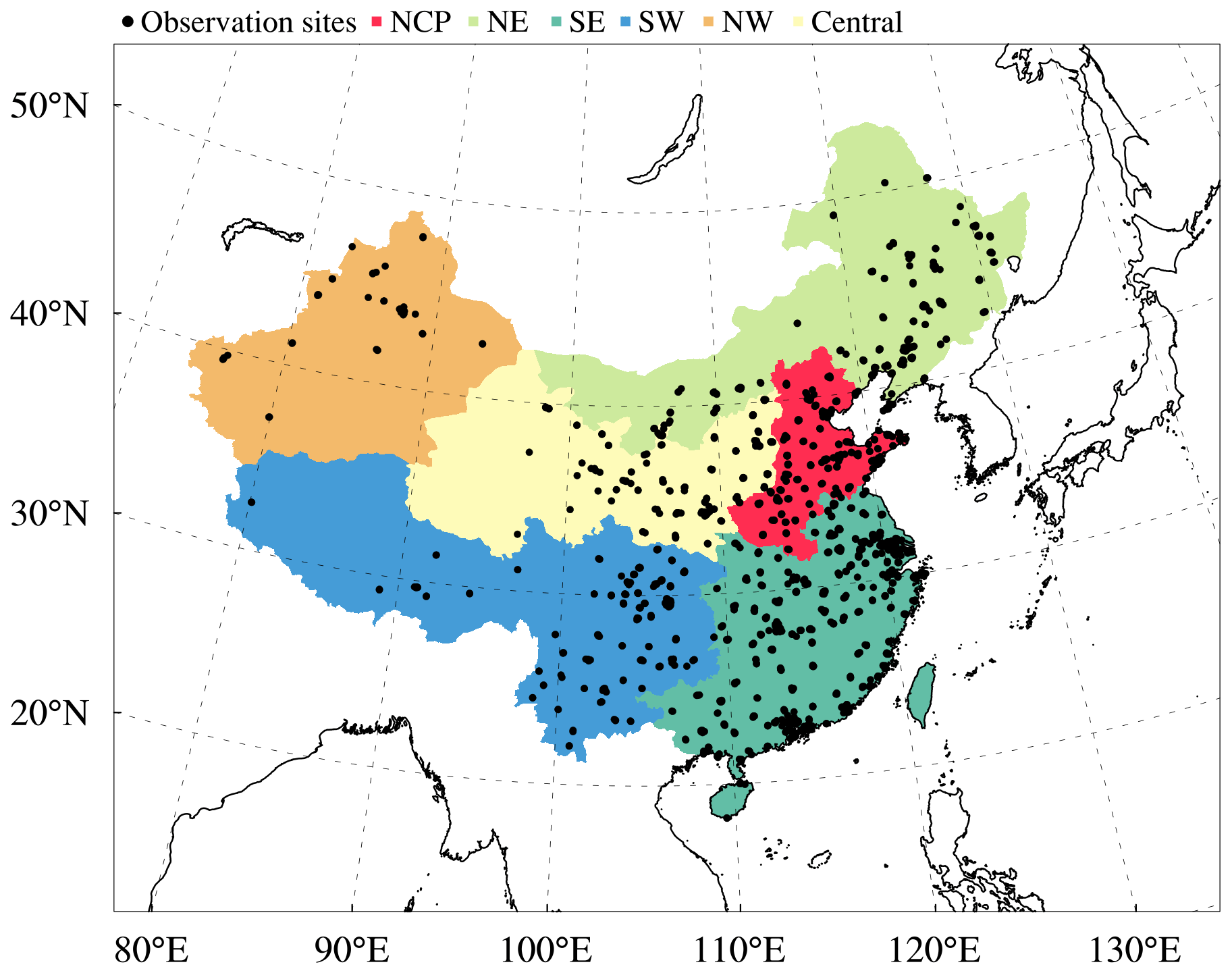
Figure 1 Modeling domain of the ensemble simulation overlaid with the distributions of observation sites from CNEMC. Different colors denote the different regions of concern in this study, i.e., the North China Plain (NCP), northeastern China (NE), southwestern China (SW), southeastern China (SE), northwestern China (NW), and central China (Central).

Figure 1 shows the domain of the inverse model, which is the same as that used in CAQRA, with a fine-scale horizontal resolution of 15 km. The HTAPv2.2 emission inventory was used as the a priori estimate of anthropogenic emissions in China and includes emissions from the energy, industry, transport, residential, agricultural, air, and shipping sectors with a base year of 2010 (Janssens-Maenhout et al., 2015). This is a harmonized global emission inventory that comprises different regional gridded inventories. Within the region of China, the air pollutant emissions were mainly provided by MEIC (Janssens-Maenhout et al., 2015). The a priori estimates of emissions from other sources include the biogenic emissions obtained from the Monitoring Atmospheric Composition and Climate (MACC) project (Sindelarova et al., 2014); biomass burning emissions obtained from the Global Fire Emissions Database (GFED), version 4 (van der Werf et al., 2010; Randerson et al., 2017); soil and lightning NO_x emissions obtained from Yan et al. (2003) and Price et al. (1997); and marine volatile organic compound emissions obtained from the POET database (Granier et al., 2005). The dust emissions were calculated online in NAQPMS as a function of the relative humidity, frictional velocity, mineral particle size distribution, and surface roughness (Li et al., 2012), while the sea salt emissions were calculated using the scheme of Athanasopoulou et al. (2008). Note that, since we aimed to estimate the air pollutant emissions and their changes from the surface observation, we did not consider the temporal variation in the a priori emission inventory. This would ensure that the top-down estimated emission trends were only derived from the surface observations, without being influenced by the trends in the prior emission inventory. In this way, our top-down estimation can serve as an independent estimation of the air pollutant emission changes in China. Meanwhile, we used the constant diurnal variation in the emissions in this study due to the lack of information on the diurnal variation in the emissions from different sectors, which is a potential limitation in our current work. However, since the emission inversion was performed on a daily basis (Sect. 2.3.3), the diurnal variations in the emission may not significantly influence the simulation results of the daily mean concentrations of air pollutants (less than 1 ppbv for SO₂, NO₂, and O₃) according to the sensitivity experiments conducted by Wang et al. (2010). The initial condition was treated as clean air in NAQPMS, with a 2-week spin-up time. Top and boundary conditions were provided by the Model for Ozone and Related Chemical Tracers (MOZART) (Brasseur et al., 1998; Hauglustaine et al., 1998) data products provided by the National Center for Atmospheric Research (NCAR). Note that, since the MOZART data products were not available for the years after 2018, the multiyear average results from 2013 to 2017 were used for the simulations after 2018. Because most of the model boundaries were set in the clean areas and are located some distance from China, we assumed that the differences in boundary conditions would not significantly affect the modeling results over China. To improve the performance of meteorological simulation, a 36 h free run of the WRF model was conducted for each day by using the NCAR/NCEP 1° × 1° reanalysis data. The simulation results of the first 12 h were treated as the spin-up run, and the remaining 24 h were used to provide the meteorological inputs for the NAQPMS model. The evaluation results for the WRF simulation are available in Sect. S1 in the Supplement, which suggests acceptable performance of the WRF simulation for the inversion estimates (Table S1 in the Supplement).

2.2 Assimilated observations

The assimilated observational dataset in this study was the same as that used in CAQRA, which includes surface concentrations of PM_2.5, PM₁₀ (coarse particulate matter), SO₂, NO₂ (nitrogen dioxide), CO, and O₃ from 2013 to 2020, obtained from CNEMC (Fig. 1). Before the assimilation, outliers of the observations were filtered out by using an automatic quality control method developed by Wu et al. (2018). Four types of outliers characterized by temporal and spatial inconsistencies, instrument-induced low variances, periodic calibration exceptions, and PM₁₀ concentrations lower than those of PM_2.5 were filtered out to prevent adverse impacts on the inversion process. As estimated in Kong et al. (2021), about 1.5 % of the observational data were filtered out after quality control, but further assessment showed that it had few effects on the average concentrations of different species, which were estimated to be less than 1 µg m⁻³ for the gaseous air pollutants and less than 5 µg m⁻³ for the particulate matter. Estimation of the observational error is also important for the inversion of emissions since the observational error and background errors determine the degree of adjustment to the emissions. The observational error comprises the measurement error and the representativeness error induced by the different spatial scales that the model and observations represent. The estimations of these two components of the observational error were the same as those used in CAQRA, detailed descriptions of which are available in Kong et al. (2021).

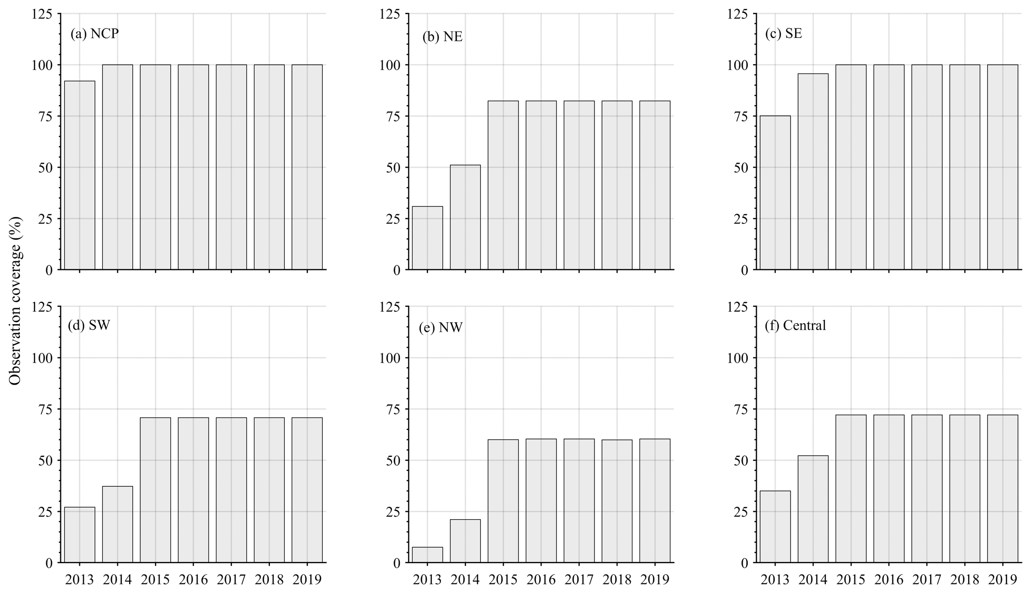
Figure 2 Time series of the observational coverage from 2013 to 2020 over different regions of China.

It should be noted that the number of observation sites was not constant throughout the whole inversion period, being approximately 510 in 2013 and then increasing to 1436 in 2015. According to Fig. S1 in the Supplement, the observation sites were mainly concentrated in the megacity clusters (e.g., the North China Plain, the Yangtze River Delta, and the Pearl River Delta) and the capital cities of each province in 2013. The number of observation sites continued to increase across China in 2014 and 2015. In particular, many areas that were previously unobserved added monitoring stations in 2014 and 2015, which significantly increased the observational coverage of China and could have led to spurious trends in the top-down estimated emissions. Figure 2 shows the changes in the observational coverage over different regions of China from 2013 to 2020, indicated by the ratio of areas that were influenced by observations to the total area of each region. It can be seen clearly that the observational coverage increased from 2013 to 2015 with the expansion of the air quality monitoring network in China and became stable after 2015. However, the influence of the variation in the number of observation sites varied among the different regions. Over the North China Plain (NCP) region, the observational coverage was approximately 90 % in 2013 and reached 100 % in 2014, suggesting that the variation in the observation sites may have little influence on the estimated emission changes there. A similar conclusion can be drawn for the southeastern China (SE) region, where the observational coverage was about 75 % in 2013 and reached 100 % in 2015. Elsewhere, in the other four regions, the influence of the variation in observation sites is expected to be larger because of the low observational coverage in both 2013 and 2014. For example, the observational coverage over the northwestern China (NW) region was less than 10 % in 2013 but increased to about 60 % in 2015. To better illustrate the impact of changes in observational coverage on the inversions, a sensitivity analysis of the emission increments with the fixed observation sites or varying observation sites is performed in this study (Sect. S2 and Fig. S2 in the Supplement). This shows that the additional emission increments caused by the increases in the number of observation sites would weaken the decreasing trends estimated in the fixed-site scenario for the emissions of PM_2.5, NO_x, and NMVOCs and even lead to increasing trends for the emissions of PM₁₀ and CO. In contrast, the increases in the number of observation sites would enhance the decreasing trends of SO₂ estimated in the fixed-site scenario. Such different behaviors are mainly related to the different signs of the emission increments of different species, as we illustrate in Sect. S2. These results highlight the significant influences of the site differences on the estimated emissions and their trends, which should be noted by potential users. Therefore, in order to reduce this influence on the estimated emission trends, in our following analysis we mainly analyze the emission trends after 2015, when the observational coverage had stabilized in all the regions.

2.3 Data assimilation algorithm

We used the modified EnKF coupled with the state augmentation method to constrain the long-term emissions of different air pollutants. The EnKF is an advanced data assimilation method proposed by Evensen (1994) that represents the background error covariance matrix with a stochastic ensemble of model realizations. Through the use of ensemble simulations, it has the ability to consider the indirect relationship between the emissions and chemical concentrations caused by the complex physical and chemical processes in the atmosphere. It also allows for the estimation of flow-dependent emission–concentration relationships that vary in time and space depending on the atmospheric conditions. The modified EnKF is an offline application of the EnKF method that works by decoupling the analysis step from the ensemble simulation, which has benefits in the reuse of costly ensemble simulations and makes high-resolution long-term inversion affordable (H. Wu et al., 2020). In this method, the ensemble simulation was first performed with the perturbed emissions, and then the observations were assimilated to constrain the emissions (H. Wu et al., 2020). The state augmentation method is a commonly used parameter estimation method (Tandeo et al., 2020) in which the air pollutant emissions are taken as the state variable and are updated according to the error covariance between the emissions and concentrations of related species.

2.3.1 State variable and ensemble generations

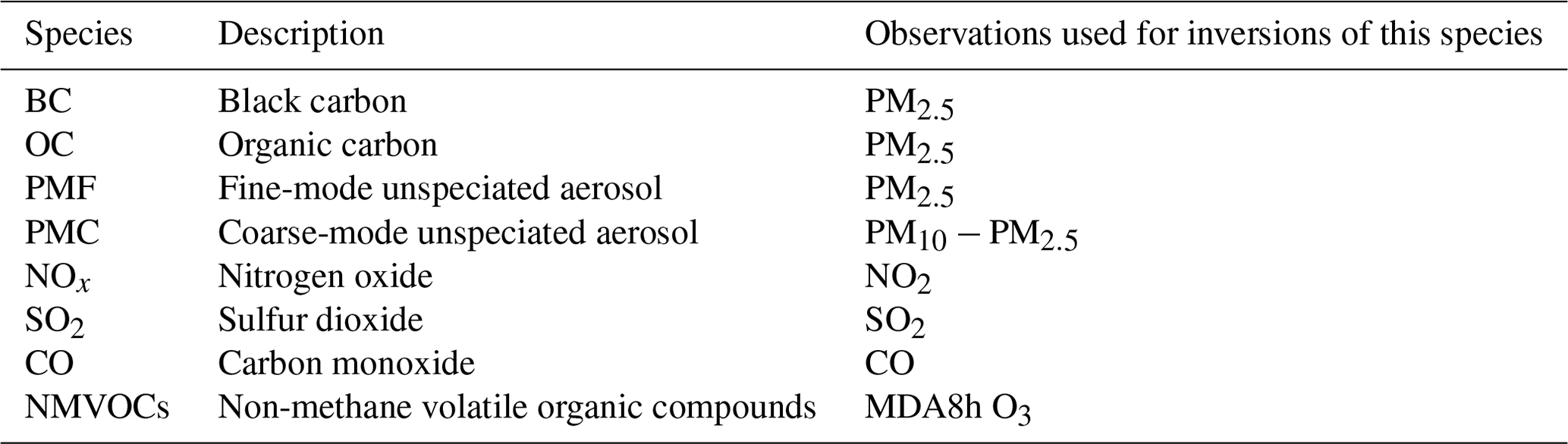
The state variable used in this study was chosen following our previous multispecies inversion study (Kong et al., 2023b), which included the scaling factors for the emissions of fine-mode unspeciated aerosol (PMF), coarse-mode unspeciated aerosol (PMC), BC, OC, NO_x, SO₂, CO, and NMVOCs as well as the chemical concentrations of PM_2.5, PM_10−2.5 (PM₁₀ minus PM_2.5), NO₂, SO₂, CO, and the daily maximum 8 h O₃ (MDA8h O₃), which are formulated as follows:

$$\begin{array}{}\text{(1)}& {\displaystyle }\mathit{x}={\left[\mathit{c},\mathit{\beta }\right]}^{\mathrm{T}},\text{(2)}& {\displaystyle }\mathit{c}=\left[{\text{PM}}_{\mathrm{2.5}},{\text{PM}}_{\mathrm{10}-\mathrm{2.5}},{\mathrm{NO}}_{\mathrm{2}},{\mathrm{SO}}_{\mathrm{2}},\mathrm{CO},\text{MDA8h}{\mathrm{O}}_{\mathrm{3}}\right],\text{(3)}& {\displaystyle }\mathit{\beta }=[{\mathit{\beta }}_{\mathrm{PMF}},{\mathit{\beta }}_{\mathrm{PMC}},{\mathit{\beta }}_{\mathrm{BC}},{\mathit{\beta }}_{\mathrm{OC}},{\mathit{\beta }}_{{\mathrm{NO}}_x}{\mathit{\beta }}_{{\mathrm{SO}}_{\mathrm{2}}}{\mathit{\beta }}_{\mathrm{CO}},{\mathit{\beta }}_{\mathrm{NMVOC}}],\end{array}$$

where x denotes the vector of the state variable, c denotes the vector of the chemical concentrations of different species, and β denotes the vector of the scaling factors for the emissions of different species. Note that, although the chemical concentration variables are included in the state variable, they are not optimized simultaneously with the emission in the analysis step and are only used to estimate the covariance between the emissions and concentrations. Detailed descriptions of the state variables are available in Table 1.

Table 1 Corresponding relationships between the chemical observations and adjusted emissions.

The ensemble of the scaling factors for different species was generated independently using the same method of Kong et al. (2021), which has a medium size of 50 and considers the uncertainties of major air pollutant emissions in China, including SO₂, NO_x, CO, NMVOCs, ammonia, PM₁₀, PM_2.5, BC, and OC. The uncertainties of these species were considered to be 12 %, 31 %, 70 %, 68 %, 53 %, 132 %, 130 %, 208 %, and 258 %, respectively, according to the estimates of M. Li et al. (2017) and Streets et al. (2003). Note that in this study we did not perturb the emissions of different sectors to reduce the degrees of freedom in the ill-posed inverse estimation problem. Instead, we only perturbed the total emissions of different species. Therefore, only the total emissions of different species were constrained in this study. The ensemble of the chemical concentrations was then generated through an ensemble simulation based on NAQPMS and the perturbed emissions calculated by multiplying the a priori emissions by the ensemble of scaling factors. This treatment implicitly assumes that the uncertainty in the chemical concentration is mainly caused by the emission uncertainty. This makes sense on a monthly or yearly basis, considering that substantial changes in emissions are expected to have taken place during the clean-air action plans, which are subject to large uncertainty. However, the lack of consideration of other error sources, such as those of the meteorological simulation and the model itself, may lead to underestimation of the background error covariance and emission adjustment, which is a potential limitation of this study. In addition, the dust and sea salt emissions were not perturbed and constrained in this study, and thus the errors in the simulated fine- and coarse-dust emissions would influence the inversion of PM_2.5 and PM₁₀ emissions. As a result, the top-down estimated PM_2.5 and PM₁₀ emissions will contain errors in the simulated dust and sea salt emissions. In particular, we did not consider the emissions of coarse dust during the inversion process since there is large uncertainty in the simulated coarse-dust emissions of current dust emission schemes (Zeng et al., 2020; Kang et al., 2011). The large errors in the simulated coarse-dust concentration could significantly influence the inversion results of PM₁₀ emissions. For example, the simulated coarse-dust concentration could sometimes be several orders of magnitude higher than the observed PM₁₀ concentration, leading to overly low values of the inverse PM₁₀ emissions (approximately 0) over the regions that were not typical dust source regions but were influenced by the transportation of coarse dust. Therefore, we only used simulated PM₁₀ concentrations from other sources in the inversion of PM₁₀ emissions to avoid the influences of the overly large errors in the simulations. This is also similar to assuming that the coarse-dust emission is equal to 0 during the assimilation. However, in this way, the top-down estimated PM₁₀ emissions in this study would comprise all coarse-dust emissions, which should be noted by potential users. A detailed description of the ensemble generation is available in Kong et al. (2021).

2.3.2 Inversion algorithm

We used a deterministic form of the EnKF (DEnKF) proposed by Sakov and Oke (2008) to update the scaling factors of the emissions of different species, which is formulated as follows:

$$\begin{array}{}\text{(4)}& {\displaystyle }\overline{{\mathit{x}}^{\mathrm{a}}}=\overline{{\mathit{x}}^{\mathrm{b}}}+\mathbf{K}\left({\mathbf{y}}^{\mathrm{o}}-\mathbf{H}\overline{x^{\mathrm{b}}}\right),\text{(5)}& {\displaystyle }{\mathbf{X}}^{\mathrm{a}}={\mathbf{X}}^{\mathrm{b}}-{\displaystyle \frac{\mathrm{1}}{\mathrm{2}}}{\mathbf{KHX}}^{\mathrm{b}},\text{(6)}& {\displaystyle }\mathbf{K}=\mathit{\lambda }{\mathbf{B}}_{\mathrm{e}}^{\mathrm{b}}{\mathbf{H}}^{\mathrm{T}}{\left(\mathbf{H}\mathit{\lambda }{\mathbf{B}}_{\mathrm{e}}^{\mathrm{b}}{\mathbf{H}}^{\mathrm{T}}+\mathbf{R}\right)}^{-\mathrm{1}},\text{(7)}& {\displaystyle }{\mathbf{B}}_{\mathrm{e}}^{\mathrm{b}}={\displaystyle \frac{\mathrm{1}}{N-\mathrm{1}}}\sum _{i=\mathrm{1}}^N{\mathbf{X}}_i^{\mathrm{b}}{\left({\mathbf{X}}_i^{\mathbf{b}}\right)}^{\mathrm{T}},\text{(8)}& {\displaystyle }\overline{{\mathit{x}}^{\mathrm{b}}}={\displaystyle \frac{\mathrm{1}}{N}}\sum _{i=\mathrm{1}}^N{\mathit{x}}_i^{\mathrm{b}};{\mathbf{X}}_i^{\mathrm{b}}={\mathit{x}}_i^{\mathrm{b}}-\overline{x^{\mathrm{b}}},\end{array}$$

where $\stackrel{\mathrm{‾}}{\mathit{x}}$ denotes the ensemble mean of the state variable; the superscripts b and a, respectively, denote the a priori and a posteriori estimates; and X^a denotes the analyzed anomalies that can be used to calculate the uncertainty of the a posteriori emissions. K is the Kalman gain matrix, ${\mathbf{B}}_{\mathrm{e}}^{\mathrm{b}}$ is the background error covariance matrix calculated by the background perturbation X^b, y^o is the vector of the observation, and R is the observational error covariance matrix. H is the linear observation operator, which maps the model space to the observation space. λ is the inflation factor used to compensate for the underestimation of the background error caused by the limited ensemble size and unaccounted-for error sources and is calculated using the method of Wang and Bishop (2003):

$$\begin{array}{}\text{(9)}& {\displaystyle }\mathit{\lambda }={\displaystyle \frac{{\left({\mathbf{R}}^{-\mathrm{1}/\mathrm{2}}\mathit{d}\right)}^{\mathrm{T}}{\mathbf{R}}^{-\mathrm{1}/\mathrm{2}}\mathit{d}-\mathit{p}}{\mathrm{trace}\left\{{\mathbf{R}}^{-\mathrm{1}/\mathrm{2}}{\mathbf{HB}}_{\mathrm{e}}^{\mathrm{b}}{\left({\mathbf{R}}^{-\mathrm{1}/\mathrm{2}}\mathbf{H}\right)}^{\mathrm{T}}\right\}}},\text{(10)}& {\displaystyle }\mathit{d}={\mathit{y}}^{\mathrm{o}}-\mathbf{H}\overline{x^{\mathrm{b}}},\end{array}$$

where d is the observation innovation and p is the number of observations. Table S2 in the Supplement summarizes the calculated average value (standard deviation) of the used inflation factor for different species. It shows that the inflation factor over eastern China (including the NCP and SE regions) was generally around 1.0, suggesting that the original ensemble can represent the simulation errors of the different air pollutants well over these regions. The inflation factor is larger over western China (including the SW, NW, and Central regions), especially for PM₁₀ (36.0–78.1) and SO₂ (7.8–176.1), suggesting that the original ensemble may underestimate the simulation errors of the air pollutants. This is associated with the large biases in the simulated air pollutant concentrations over there and shows that the emission uncertainties assumed in our studies may be underestimated over these regions. This also highlights the importance of the use of the inflation method during the inversion; otherwise, it would lead to filter divergency caused by the underestimations of the background error covariance.

In order to reduce the influence of the spurious correlations on the performance of data assimilation, the EnKF was performed locally in this study in that the analysis was calculated grid by grid with the assumption that only measurements located within a certain distance (cutoff radius) from a grid point would influence the analysis results of this grid. The use of this local analysis method also allowed the inflation factor to be calculated locally and to vary in time and space, which can help characterize the spatiotemporal variations in errors, as we illustrated above. Similarly to Kong et al. (2021) and Kong et al. (2023b), the cutoff radius was chosen as 180 km for each species based on the wind speed and the lifespan of the species (Feng et al., 2020). The same local scheme with a buffer area was also employed during the inversion to alleviate the discontinuities in the updated state caused by the cutoff radius. A detailed description of the local analysis scheme is available in Kong et al. (2021).

Table 1 summarizes the corresponding relationships between the emissions and chemical concentrations. Similarly to Ma et al. (2019) and Miyazaki et al. (2012), we did not consider the interspecies correlation during the assimilation to prevent the spurious correlations between unrelated or weakly related variables. In most cases, observations of one particular species were only allowed to adjust emissions of the same species. The assimilation of PM_2.5 mass observation was more complicated as there are multiple error sources in the simulated mass concentrations of PM_2.5, not only from primary emission, but also from secondary production. In this study, the PM_2.5 mass observation was used to constrain the emissions of PMF, BC, and OC but was not used to constrain the emissions of its precursors to avoid the spurious correlations and nonlinear chemistry effects, similar to the scheme used in Ma et al. (2019). This is feasible as the emissions of primary PM_2.5 (i.e., PMF, BC, and OC) and the emissions of PM_2.5 precursors (e.g., SO₂, NO₂) were perturbed independently in our method, and thus the contributions of primary PM_2.5 emissions and secondary PM_2.5 productions to PM_2.5 mass could be isolated through the use of ensemble simulations. Meanwhile, the use of the iteration inversion method (which will be introduced later) can further reduce the influence of the errors in the precursors' emissions on the inversion of primary PM_2.5 emissions, because the errors of the precursors' emissions would be constrained by their own observations during the iterations. However, the lack of assimilation of speciated PM_2.5 observations may lead to uncertainties in the estimated emissions of PMF, BC, and OC, which is a potential limitation in the current work. For example, if the a priori simulated PM_2.5 equals the observations, the emissions of PMF, BC, and OC would not be adjusted by using the current method. However, in such cases, there may still be errors in the proportions of the emissions of different PM_2.5 components. To adjust the emissions of PMC, we used the observations of PM_10−2.5 to avoid the potential cross-correlations between PM_2.5 and PM₁₀ (Peng et al., 2018; Ma et al., 2019). For the NO_x emissions, although the O₃ concentrations are chemically related to the NO_x emissions, we did not use the O₃ concentrations to constrain the NO_x emissions in this study as there is a nonlinear relationship between O₃ concentration and NO_x emission, which would lead to incorrect adjustment of NO_x emissions (Tang et al., 2016).

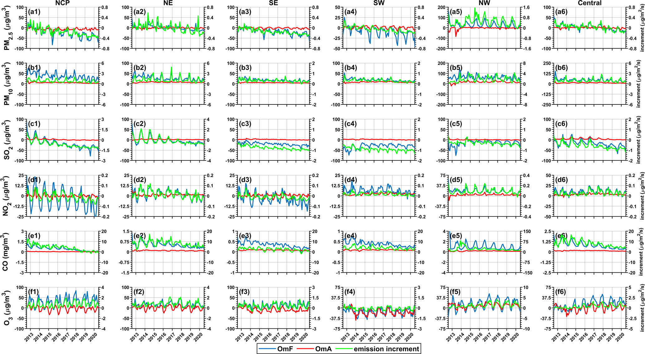
Figure 3 Time series of the a priori bias (blue lines), the a posteriori bias (red lines), and the emission increment (green lines) from 2013 to 2020 for the different species over the six regions of China.

The inversion of NMVOC emissions is more difficult than that of other species due to the lack of long-term nationwide NMVOC observations and the strong chemical activity. Previous studies usually assimilated satellite observations of formaldehyde and glyoxal to constrain NMVOC emissions, such as Cao et al. (2018) and Stavrakou et al. (2015). However, these inversion studies were hindered by the NO_x–VOC–O₃ chemistry and the inherent uncertainty in satellite observations of formaldehyde and glyoxal. Considering the strong chemical relationship between O₃ and NMVOCs, some pioneering studies also explored the method of assimilating ground-level O₃ concentrations to constrain NMVOC emissions (Ma et al., 2019; Xing et al., 2020) and demonstrated the effectiveness of this approach. For example, Ma et al. (2019) found that the assimilation of O₃ concentrations could adjust NMVOC emissions in the direction of the bottom-up inventories, and the forecast skills of the O₃ concentrations were also improved, indicating that the constrained NMVOC emissions were improved relative to their a priori values. Inspired by these studies, we have made an attempt to constrain NMVOC emissions based on MDA8h O₃. The use of MDA8h O₃ rather than the daily mean O₃ concentration is meant to avoid the effects of the nighttime O₃ chemistry. For example, the simulation errors in the titration effects of NO_x may influence the simulated O₃ concentrations at night and affect the inversion results of the NMVOCs. An important issue that should be noted when using MDA8h O₃ to constrain the NMVOC emissions is the nonlinear interactions between NO_x, NMVOCs, and O₃. On the one hand, the O₃ concentrations are dependent on not only the NMVOC emissions, but also the NO_x emissions. The errors in the a priori emissions of NO_x would also contribute to the simulation errors of O₃ and deteriorate the inversion of the NMVOCs. The iteration inversion scheme could help deal with this issue as the errors in the NO_x emissions will be constrained by the NO₂ observations in the next iteration, which can reduce the influences of errors in the NO_x emission on the inversion of NMVOC emissions based on MDA8h O₃ concentrations. This is in fact similar to the approach used by Xing et al. (2020), who first constrained the NO_x emissions based on observations of NO₂ and then constrained the NMVOC emissions based on O₃ concentrations. Also, in Feng et al. (2024), the NO₂ observations were simultaneously assimilated to constrain the NO_x emissions to account for the influences of errors in the NO_x emissions on the NMVOC emissions, suggesting that the iteratively nonlinear joint inversion of NO_x and NMVOCs is an effective way of addressing the intricate relationship between VOC, NOx, and O₃ (Feng et al., 2024). Similarly, the errors in the CO emissions, which may be significant according to our following analysis, are also constrained in a similar way to reduce the potential influences on the inversion of the NMVOC emissions. On the other hand, the emission adjustments of NMVOCs may exhibit bidirectionality that is dependent on the VOC-limited or NO_x-limited regimes. According to Fig. 3, the NMVOC emissions were adjusted in alignment with the direction of the O₃ errors, suggesting a VOC-limited regime over urban areas in China, given that the O₃ observation sites are predominantly situated in urban areas. This is in agreement with Ren et al. (2022), who diagnosed the NO_x–VOC–O₃ sensitivity based on the satellite retrievals and found that the VOC-limited regimes are mainly located in urban areas in China. This suggests that the relationship between the O₃ concentrations and VOC emissions could be reasonably reflected by our inversion system, providing the feasibility of utilizing the O₃ observations to constrain the VOC emissions. Note that, due to the lack of observations of VOC components, we only optimize the gross emissions of the VOCs during the assimilation.

As we illustrated before, there exist nonlinear effects in the atmospheric chemistry which could influence the inversion results of different species. In addition, since we did not consider the temporal variations in the a priori emissions, it was expected that there would be significant biases in the a priori emissions for the years after 2013, as substantial changes in emissions were expected owing to the implementation of strict emission control measures. Such bias in the a priori emissions does not conform to the unbiased hypothesis of the EnKF, which could lead to incomplete adjustments of the a priori emissions and degrade the performance of the data assimilation (Dee and Da Silva, 1998). To address these issues, an iteration inversion scheme that was used previously in Kong et al. (2023b) was employed in this study. The main ideas of the iteration inversion scheme are to preserve the background perturbation X^b and to update the ensemble mean of the state variable $\overline{{\mathit{x}}^{\mathrm{b}}}$ based on the model simulations driven by the inversion results of the kth iteration. Therefore, a new single model simulation needs to be conducted by using the a posteriori emission from the previous iteration as the input to update the ensemble mean of the original ensemble. This enables the observational information and the adjusted emissions to be promptly incorporated into the model, thereby providing feedback for the adjustments of emissions in the next iteration. However, we did not reassemble the ensemble simulation for each iteration due to the expensive computational cost of the ensemble simulation. Therefore, in each iteration calculation, the ensemble perturbations that were used to calculate the background error covariance matrix remain the same, with only the ensemble mean being updated based on the inversion results of the previous iteration. The state variable used in the (k+1)th inversions is then formulated as follows:

$$\begin{array}{}\text{(11)}& {\mathit{x}}_i^{\mathrm{b},k+\mathrm{1}}={\left[{\mathit{c}}^k+{\mathit{c}}_i^{\mathrm{e}}-\overline{{\mathit{c}}^{\mathrm{e}}},{\mathit{\beta }}^k+{\mathit{\beta }}_i^{\mathrm{e}}-\overline{{\mathit{\beta }}^e}\right]}^{\mathrm{T}},\end{array}$$

where c^k represents the model simulations driven by the inversed emissions of the kth iteration, $c_i^{\mathrm{e}}$ represents the ith member of ensemble simulations with an ensemble mean of $\overline{{\mathit{c}}^{\mathrm{e}}}$, β^k represents the updated scaling factors of the kth iteration, and ${\mathit{\beta }}_i^{\mathrm{e}}$ represents the ith member of the ensemble of scaling factors with a mean value of $\overline{{\mathit{\beta }}^{\mathrm{e}}}$. In each iteration, all emissions are updated simultaneously, and two rounds of iterations were conducted in this study based on our previous inversion study to maintain a balance between the inversion performance and the computational cost of the long-term inversions (Kong et al., 2023b).

2.3.3 Setup of inversion estimation

Based on this inversion scheme, we constrained the daily emissions of PMF, PMC, BC, OC, NO_x, SO₂, CO, and NMVOCs from 2013 to 2020, based on the daily averaged observations of PM_2.5, PM_10−2.5, NO₂, CO, and MDA8h O₃. However, due to the lack of enough speciated PM_2.5 observations, the model performance driven by the inversed emission for the BC, OC, and primary unspeciated PM_2.5 has not been evaluated thoroughly. It is thus currently unclear for the quality of the inversed emissions of BC, OC, and primary unspeciated PM_2.5. Also, the lack of speciated PM_2.5 observations could lead to uncertainties in the estimated emissions of PMF, BC, and OC, as we mentioned before. Considering this, similar to Kong et al. (2023b), although we made an attempt to estimate the emissions of BC, OC, and primary unspeciated PM_2.5, we have reservations about their inversion results and only provide the emissions of PM_2.5 (PMC + BC + OC) and PM₁₀ (PM_2.5 + PMC) in the current stage. In the future, we will collect more speciated PM_2.5 observations to comprehensively quantify the accuracy of their inversion results, after which the emissions of these species will be released. Meanwhile, the speciated PM_2.5 observations could be assimilated in the current inversion framework. This could provide us with further constraints on the emissions of BC, OC, and primary PM_2.5. Meanwhile, as mentioned in Sect. 2.3.1, the meteorological and model uncertainties were not considered in the ensemble simulation. Thus, the errors in the meteorological simulation would cause fluctuations in the daily emissions that contaminate the inversion results and are difficult to isolate from the inherent variations in emissions (Tang et al., 2013). Considering this, the daily emissions were averaged to monthly values to reduce the influences of random model errors after the assimilation.

3 Performance of the chemical data assimilation system

3.1 Analysis of the observation minus forecast (OmF) and the emission increment

The OmF and the emission increment (a posteriori emission minus a priori emission) were first analyzed to demonstrate the performance of the data assimilation. As shown in Fig. 3, the a priori simulation generally underestimated the PM_2.5 concentrations over the NCP, SE, and SW regions (positive OmF values) during 2013–2014 but overestimated the PM_2.5 concentrations from 2016, reflecting the effects of the emission control measures during these years. In the NE, NW, and central China (hereafter “Central”) regions, obvious underestimation of the PM_2.5 concentration was found (positive OmF values) throughout almost the entire assimilation period. Similarly, the OmF values of PM₁₀ were positive throughout the whole assimilation period over all the regions of China. In contrast, the OmF values for SO₂ were negative for most of the regions, and the negative OmF values over the NCP region became larger as the years progressed, which reflects the effects of the emission control measures. The OmF for NO₂ reveals a seasonal variation over the NCP and SE regions, with negative values during summer and positive values during winter, while there were obvious positive OmF values over the NE, SW, NW, and Central regions. In terms of CO, large positive OmF values were found over all the regions of China, and there were decreasing trends in the OmF values of CO over different regions of China that were associated with the emission control policies during these years. The OmF values for O₃ were positive over most regions of China, except for the NW region. These results provide us with valuable information on the potential deficiencies in the a priori emissions. However, since our inversion method did not differentiate between anthropogenic and natural emissions, the biases in the model simulation may also be attributable to the errors in natural emissions such as dust, especially over the major dust source areas of China (e.g., the NW and Central regions). In addition, the effects of emission control were not considered in the a priori emissions, which form another important contributor to the errors in the model simulation for the later years. Thus, the emission increments calculated by the assimilation should reflect the combined effects of errors in the anthropogenic and natural emissions as well as the emission control.

The calculated emission increments were consistent with the OmF values for all the species, which indicates that the data assimilation method can probably constrain the emissions based on the observations. According to Fig. 3, the emission increments were positive for PM_2.5 over the NE, NW, and Central regions; for NO₂ over the NE, SW, NW, and Central regions; and for PM₁₀, CO, and NMVOCs over almost all the regions throughout the assimilation period. In contrast, the emission increments were negative for the SO₂ emissions in most of the cases. Consistent with the OmF values, the emission increments were positive for PM_2.5 over the NCP, SE, and SW regions during 2013–2014 but became negative from 2016 owing to the implementation of strict emission control measures. The emission increments for NO_x also showed significant seasonal variation over the NCP and SE regions, being positive during winter and negative during summer. The a posteriori biases for the model simulations of different species were also plotted to assess the performance of the data assimilation. It can be seen clearly that the biases were substantially reduced for all the species and the calculated root-mean-square errors (RMSEs) reduced by 23.2 %–52.8 % for PM_2.5, 19.9 %–37.8 % for PM₁₀, 36.4 %–77.3 % for SO₂, 18.3 %–25.2 % for NO₂, 29.9 %–40.5 % for CO, and 4.4 %–26.1 % for O₃ over the different regions of China, suggesting good performance of the data assimilation system.

Table 2 Evaluation statistics of the a posteriori (a priori) model simulation for different species^∗.

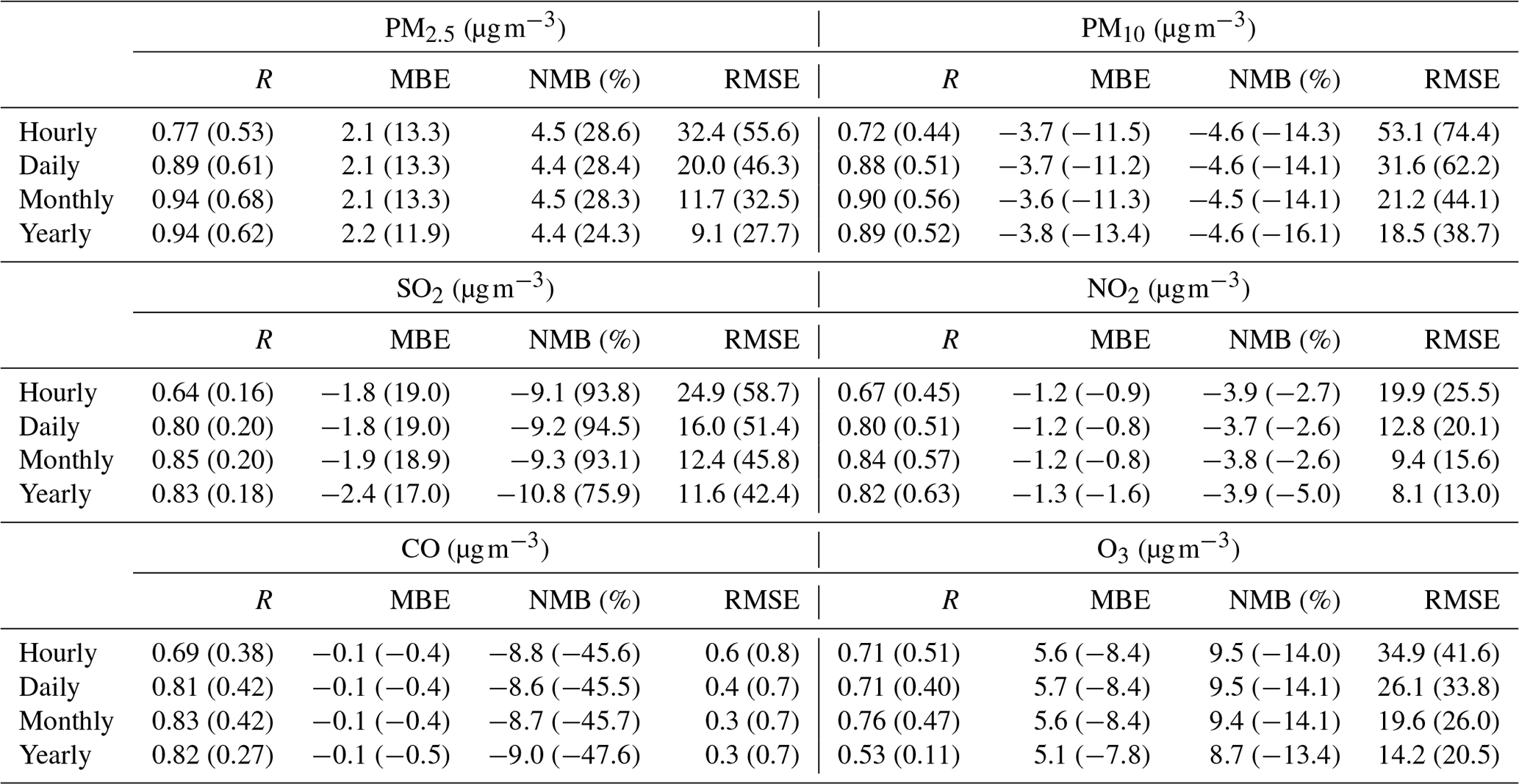
^∗ The time series of the air pollutant concentrations at each station were first catenated into a single vector. Then the values of each evaluation metric were calculated based on the catenated time series of the observed and simulated concentrations.

3.2 Evaluation of the inversion results

Table 2 shows the calculated evaluation statistics for the inversion at different temporal scales. It can be seen clearly that the model simulation with the a posteriori emission inventory reproduced the magnitude and temporal variations in the different air pollutants in China well, with calculated correlation coefficients of approximately 0.77, 0.72, 0.64, 0.67, 0.69, and 0.71 and normalized mean biases of approximately 4.5 %, −4.6 %, −9.0 %, −3.9 %, −8.8 %, and 9.5 % for the hourly concentrations of PM_2.5, PM₁₀, SO₂, NO₂, CO, and O₃, respectively. Moreover, the a posteriori model simulation achieved comparable accuracy to the air quality reanalysis data we developed in Kong et al. (2021) in terms of the RMSEs, which were 32.4, 53.1, 24.9, 19.9, 0.56, and 34.9 µg m⁻³, respectively, for these species at the hourly scale. At the daily, monthly, and yearly scales, the constrained model simulation performed better, with RMSEs of approximately 9.1–20.0 µg m⁻³ (PM_2.5), 18.5–31.6 µg m⁻³ (PM₁₀), 11.5–16.0 µg m⁻³ (SO₂), 8.1–12.8 µg m⁻³ (NO₂), 0.28–0.39 µg m⁻³ (CO), and 14.2–26.1 µg m⁻³ (O₃), which were reduced by 56.7 %–67.3 %, 49.2 %–52.1 %, 68.8 %–72.8 %, 36.3 %–39.8 %, 47.0 %–58.0 %, and 22.9 %–30.5 %, respectively, compared to the RMSEs of the a priori simulations. We also compared the model performance driven by the inversed inventory with that driven by more recent bottom-up inventories (MEIC and HTAPv3) by taking the simulation results of the year 2020 as an example to give us a more objective understanding of the accuracy of the inversed emission inventory. This shows that the inversed emission generally achieves better performance in simulating the air pollutant concentrations in China than MEIC and HTAPv3 (Table S3 in the Supplement). It is also encouraging to find that the model performance driven by CAQIEI and MEIC–HTAPv3 is similar for PM_2.5, PM₁₀, and SO₂ over the NCP, NE, SE, and SW regions, which is a significant improvement on the a priori emission inventory. This suggests that both the top-down and recent bottom-up emission inventories have good performance in capturing the emission changes in these species over these regions and that they yield consistent estimations. Detailed information on the configurations of the model simulation results driven by MEIC–HTAPv3 together with the comparison results are available in Sect. S3 in the Supplement. All these validation results confirm the good performance of the data assimilation method and suggest that the inversed emission inventory has the ability to reasonably represent the magnitude and long-term trends of the air pollutant emissions in China during 2013–2020.

4 Results

Based on the top-down estimation, the gridded emissions for PM_2.5, PM₁₀, SO₂, CO, NO_x, and NMVOCs over China from 2013 to 2020 were developed into what we have called CAQIEI. In the following sections, we first analyze the magnitude and seasonality of the air pollutant emissions in China by taking 2015 as a reference year when the number of observation sites became stable. After that, the changes in emissions of different air pollutants from 2015 to 2020 are analyzed and compared between the two clean-air action plans in China. Note that, due to the impacts of the changes in observational coverage, it is difficult to estimate the overall emission reduction rates during the 2013–2017 action plan by using our inversion results. The emission change rates during 2015–2017 are then sampled in this study to assess the mitigation effects during the 2013–2017 action plan and to compare them with the emission change rates during 2018–2020. Finally, CAQIEI is compared with the previous bottom-up and top-down emission inventories to validate our top-down estimation and to identify the potential uncertainties in the current understanding of China's air pollutant emissions.

Table 3 Inversion-estimated emissions (Tg yr⁻¹) of different species in China as well as the six regions for the year 2015.

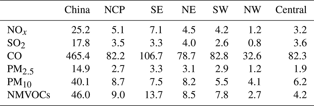
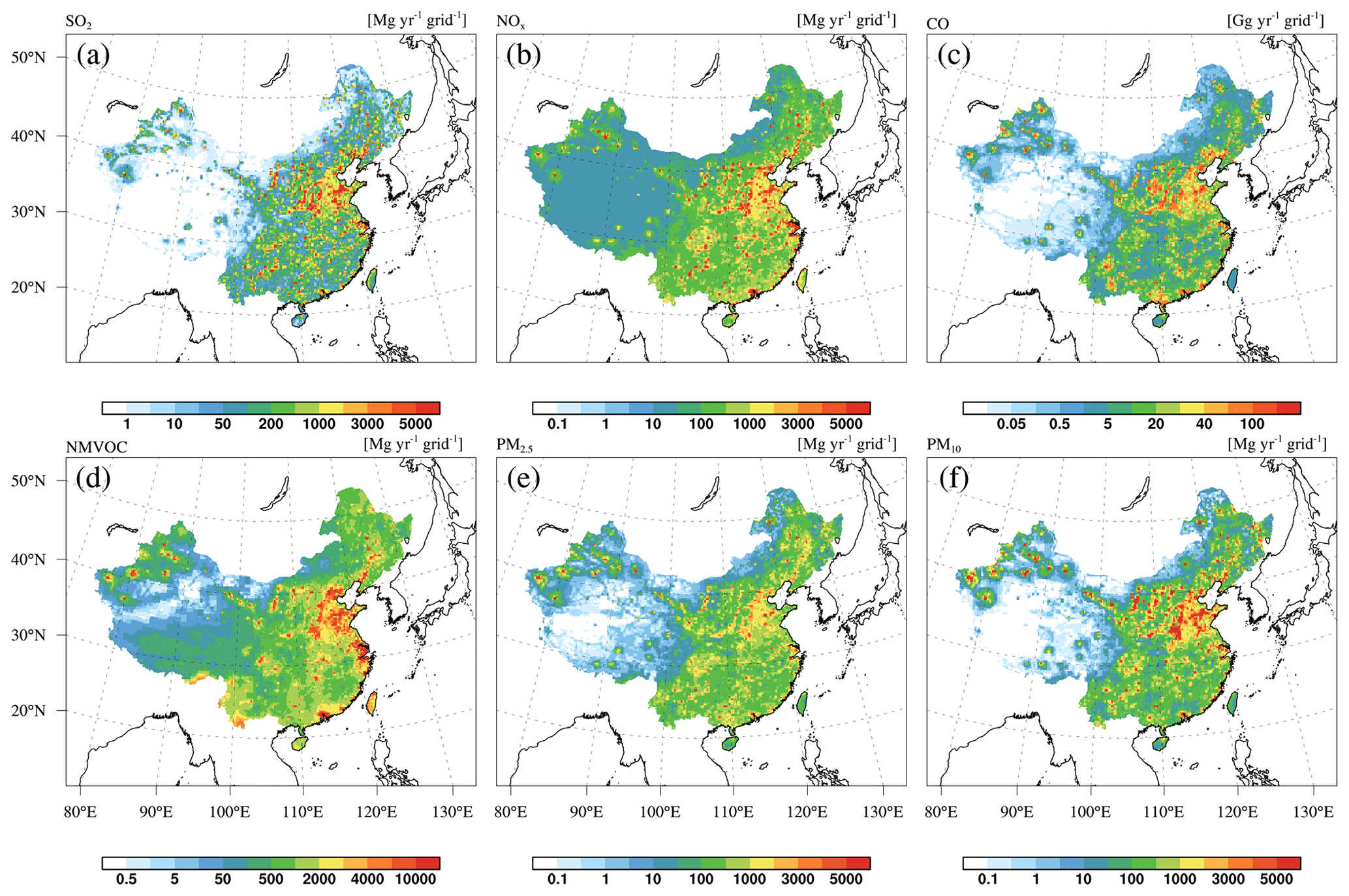
Figure 4 Spatial distributions of the emissions of (a) SO₂, (b) NO_x, (c) CO, (d) NMVOCs, (e) PM_2.5, and (f) PM₁₀ in 2015 obtained from CAQIEI.

4.1 Top-down estimated Chinese air pollutant emissions in 2015

The top-down estimated emissions of different species in 2015 are as follows: 25.2 Tg of NO_x, 17.8 Tg of SO₂, 465.4 Tg of CO, 15.0 Tg of PM_2.5, 40.1 Tg of PM₁₀, and 46.0 Tg of NMVOCs. Note that these values contain not only anthropogenic emissions, but also natural emissions (e.g., dust and biogenic NMVOCs). Thus, the top-down estimated emissions of PM and NMVOCs were higher than those estimated by previous studies, as we mention in the following sections. Emission maps of all species in 2015 are shown in Fig. 4, and the calculated emissions of different species over different regions are presented in Table 3. According to Fig. 4, higher air pollutant emissions are widely distributed in the megacity clusters (e.g., NCP, the Yangtze River Delta, and the Pearl River Delta) and developed cities in China, reflecting the influences of human activities. The NCP was the region with the highest emission intensity of air pollutants in China, contributing 5.1 Tg of NO_x, 3.5 Tg of SO₂, 82.2 Tg of CO, 2.7 Tg of PM_2.5, 8.7 Tg of PM₁₀, and 9.0 Tg of NMVOCs to the total emissions in China. The inversion results also demonstrate the contributions of natural sources to the air pollutant emissions, such as the soil NO_x emissions and the biogenic NMVOC emission distributed in the Tibetan Plateau region. In general, the majority of the air pollutant emissions were located in eastern China (including the NCP, NE, and SE regions), where the economy is relatively well developed, which in total accounted for 66.0 % of NO_x, 60.9 % of SO₂, 57.5 % of CO, 60.4 % of PM_2.5, 60.5 % of PM₁₀, and 67.8 % of NMVOC emissions in China. However, although the gross domestic product (GDP) of western China (including the SW, NW, and Central regions) is less than one-third that of eastern China, the top-down estimation indicates that the air pollutant emissions in western China could have accounted for about 32.2 %–42.5 % of the total emissions, which reflects the low emission control levels over these regions.

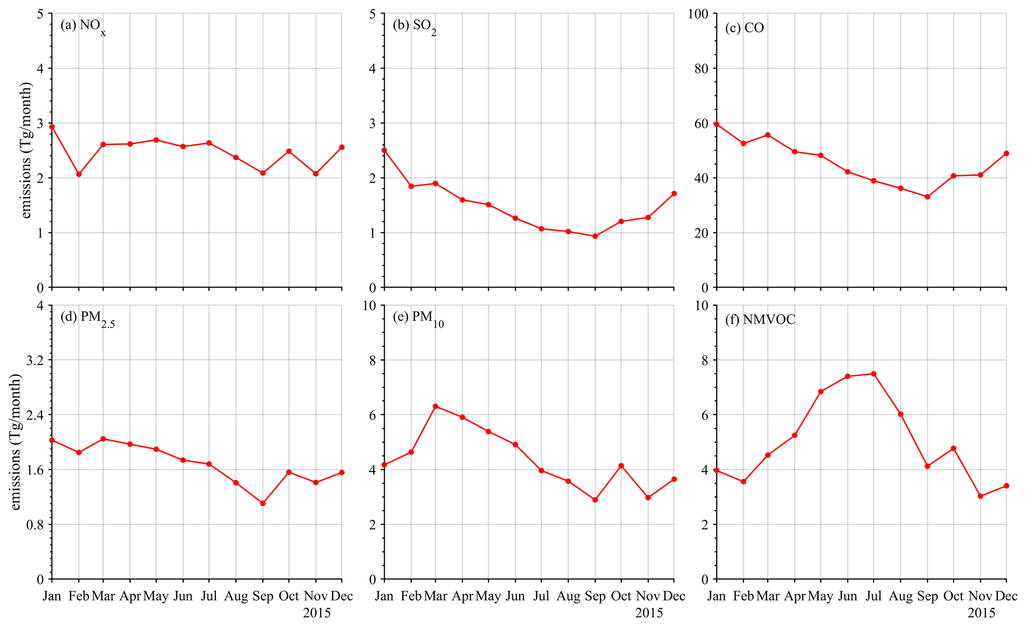
Figure 5 Monthly series of the total emissions of (a) NO_x, (b) SO₂, (c) CO, (d) PM_2.5, (e) PM₁₀, and (f) NMVOCs in China for the year 2015 obtained from CAQIEI.

Figure 5 shows the monthly variations in air pollutant emissions in China for the year 2015. The monthly profile of NO_x emissions was relatively flat among the six species. SO₂ and CO showed higher emissions during winter because of the enhanced residential emissions associated with higher coal consumption for heating during that time of the year. Meanwhile, the emission factor for CO from vehicles in winter was also higher than in the other seasons, due to additional emissions from the cold-start process (Kurokawa et al., 2013; M. Li et al., 2017). PM_2.5 and PM₁₀ had higher emissions during winter and spring, which on the one hand was due to the enhanced emissions from the residential and industrial sectors during the winter season (M. Li et al., 2017) and on the other hand the enhanced dust emissions during the spring season (Fan et al., 2021). Emissions of NMVOCs exhibited strong monthly variations, with higher emissions mainly in summer because of the enhanced NMVOC emissions from biogenic sources.

Table 4 The calculated annual trends of PM_2.5 and PM₁₀ emissions in China based on CAQIEI.

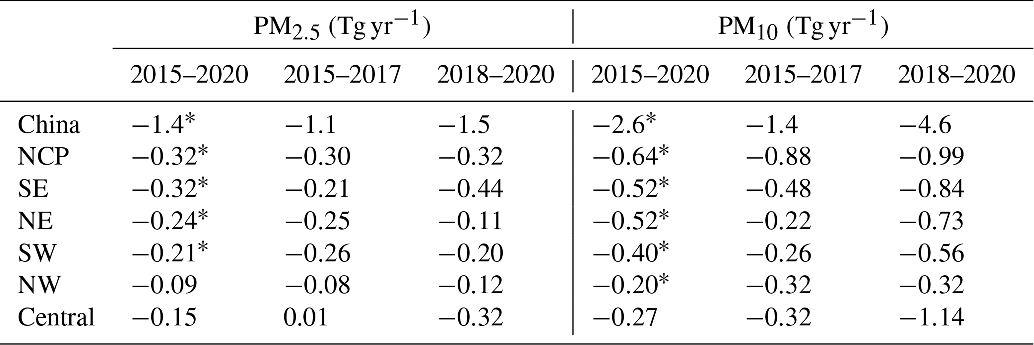
^∗ The trend is significant at the 0.05 significance level.

Figure 6 Emission changes in (a) PM_2.5 and (b) PM₁₀ obtained from CAQIEI from 2013 to 2020.

4.2 Top-down estimated emission changes in different air pollutants

4.2.1 Emission changes in particulate matter

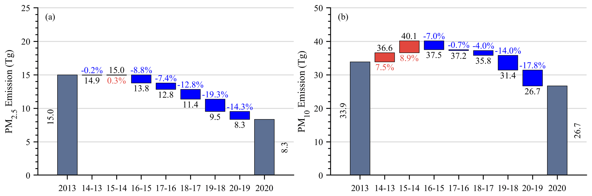
Figure 6 shows the top-down estimated emission changes in PM_2.5 and PM₁₀ over China during the two clean-air action periods. Both PM_2.5 and PM₁₀ emissions decreased substantially, by 44.3 % and 21.2 %, respectively, from 2013 to 2020. By contrast, the top-down estimates showed increases in PM_2.5 and PM₁₀ emissions in 2014 and 2015, but this would be a spurious trend caused by the changes in observation sites that we discussed in Sect. S2. Therefore, the emissions in 2013 and 2014 were discarded to prevent the spurious trends. According to Fig. 6, the PM_2.5 emissions decreased by 14.5 % from 2015 (15.0 Tg) to 2017 (12.8 Tg), and the reduction in emissions was roughly uniform throughout the period, which was about 8 % compared to the previous years. The PM₁₀ emissions showed a smaller reduction rate (−7.2 %) than that of PM_2.5, decreasing from 40.1 Tg in 2015 to 37.2 Tg in 2017. Compared with the emission reduction rate during 2015–2017, both PM_2.5 and PM₁₀ showed higher emission reduction rates during 2018–2020, which were estimated to be 27.2 % and 25.5 %, respectively. The emission reductions in each year were also larger, especially for PM₁₀. For example, PM_2.5 and PM₁₀ emissions decreased by about 19.3 % and 14.0 % in 2019 compared to 2018. This may have been due to the fact that, in addition to the strict controls imposed on the industrial and power sectors during the 2013–2017 action period, the residential emissions were strengthened during the 2018–2020 action period. In particular, “coal-to-electricity” and “coal-to-gas” strategies were vigorously implemented in northern China during the 2018–2020 action to reduce coal consumption and related air pollutant emissions (Liu et al., 2016; S. Wang et al., 2020). Thus, our inversion results confirm the effectiveness of the controls on residential emissions in terms of reducing the emissions of PM_2.5 and PM₁₀. In addition, the control of non-point sources, such as blowing-dust emissions, was also strengthened during the 2018–2020 action period, which is consistent with the faster reduction in PM₁₀ emissions during 2018–2020. The annual trends of PM_2.5 and PM₁₀ emissions were also calculated in China using the Mann–Kendall trend test and the Theil–Sen trend estimation method, the results of which are summarized in Table 4. The calculation of emission trends can help extend the existing emission datasets forward in time to produce up-to-date products. The top-down estimated trends of PM_2.5 and PM₁₀ emissions were −1.4 and −2.6 Tg yr⁻¹ during 2015–2020, which is attributable to the strict emission control measures imposed during the two clean-air action plans. As mentioned, the decreasing trends were higher during 2018–2020 (−1.5 and −4.6 Tg yr⁻¹) than during 2015–2017 (−1.1 and −1.5 Tg yr⁻¹).

On the regional scale (Fig. S3 in the Supplement), it can be seen clearly that the PM_2.5 emissions decreased consistently over all the regions (by 59.8 % in NCP, 49.6 % in SE, 39.5 % in NE, 35.8 % in SW, 33.2 % in NW, and 41.0 % in Central) from 2015 to 2020. The NCP region showed the largest reduction in emissions among the six regions, with its emission reduction rate being almost larger than 10 % in each year. This is consistent with the strictest emission control policies having been imposed over the NCP region. The SE region showed a similar emission reduction to the NCP region, with its emission reduction rate being larger than 10 % in most of the years. Obvious increases in PM_2.5 emissions were found over the NW region from 2013 to 2015 owing to the increase in the number of observation sites in those years. After 2015, PM_2.5 emissions generally decreased over the NW region, while there was a slight rebound in PM_2.5 emissions in 2016 and 2018, possibly due to the influences of the errors in fine-dust emission. The Central region showed different characteristics of emission changes to the other regions insofar as it showed little change in PM_2.5 emissions during 2015–2018 but large reductions in 2019. This may be consistent with the control of emissions over the Fenwei Plain area (the part of the Central region where the emission intensity is highest) being weak during the 2013–2017 action plan but strengthened during the 2018–2020 action plan. In terms of the PM_2.5 emission trends over the different regions, the calculated PM_2.5 emission trends were about −0.32 Tg yr⁻¹ in NCP, −0.32 Tg yr⁻¹ in SE, −0.24 Tg yr⁻¹ in NE, −0.21 Tg yr⁻¹ in SW, −0.09 Tg yr⁻¹ in NW, and −0.15 Tg yr⁻¹ in Central from 2015 to 2020.

The changes in PM₁₀ emissions were generally similar to those of PM_2.5, i.e., with decreases in all the regions from 2015 to 2020 (Fig. S4 in the Supplement). The top-down estimated PM₁₀ emission reductions from 2015 to 2020 were about 3.5 Tg (40.0 %) in NCP, 2.6 Tg (35.5 %) in SE, 3.0 Tg (36.6 %) in NE, 2.0 Tg (35.9 %) in SW, 1.0 Tg (25.3 %) in NW, and 1.3 Tg (21.6 %) in Central. The calculated trends were about −0.64, −0.52, −0.51, −0.40, −0.20, and −0.27 Tg yr⁻¹, respectively. However, due to the influences of the changes in the number of observation sites, the PM₁₀ emissions over the NE, SW, and NW regions increased substantially from 2013 to 2015, while they decreased in almost all the years after 2015. Different from the other regions, the Central region showed increases in PM₁₀ emissions from 2015 to 2018 of about 0.92 Tg (14.9 %) but substantial decreases in 2019 and 2020. The result also shows that most PM₁₀ emission reductions were achieved during the 2018–2020 action plan. According to CAQIEI, the PM₁₀ emissions decreased by 0.64–2.3 Tg (17.4 %–31.8 %) from 2018 to 2020, which accounted for 48.4 %–169.0 % of the total reduction in emissions from 2015 to 2020. This again emphasizes the effectiveness of the control of blowing-dust emissions during the 2018–2020 action plan.

Table 5 The calculated annual trends of the four gaseous emissions in China based on CAQIEI.

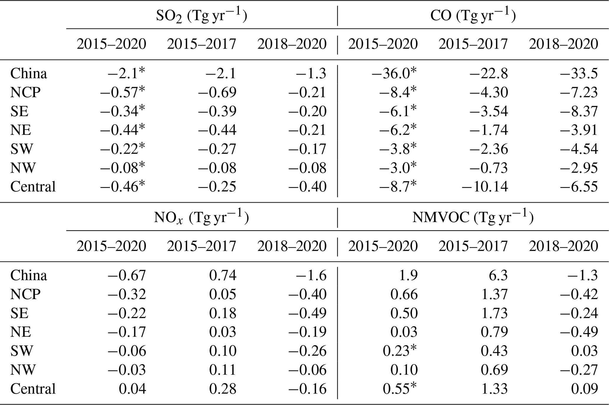
^∗ The trend is significant at the 0.05 significance level.

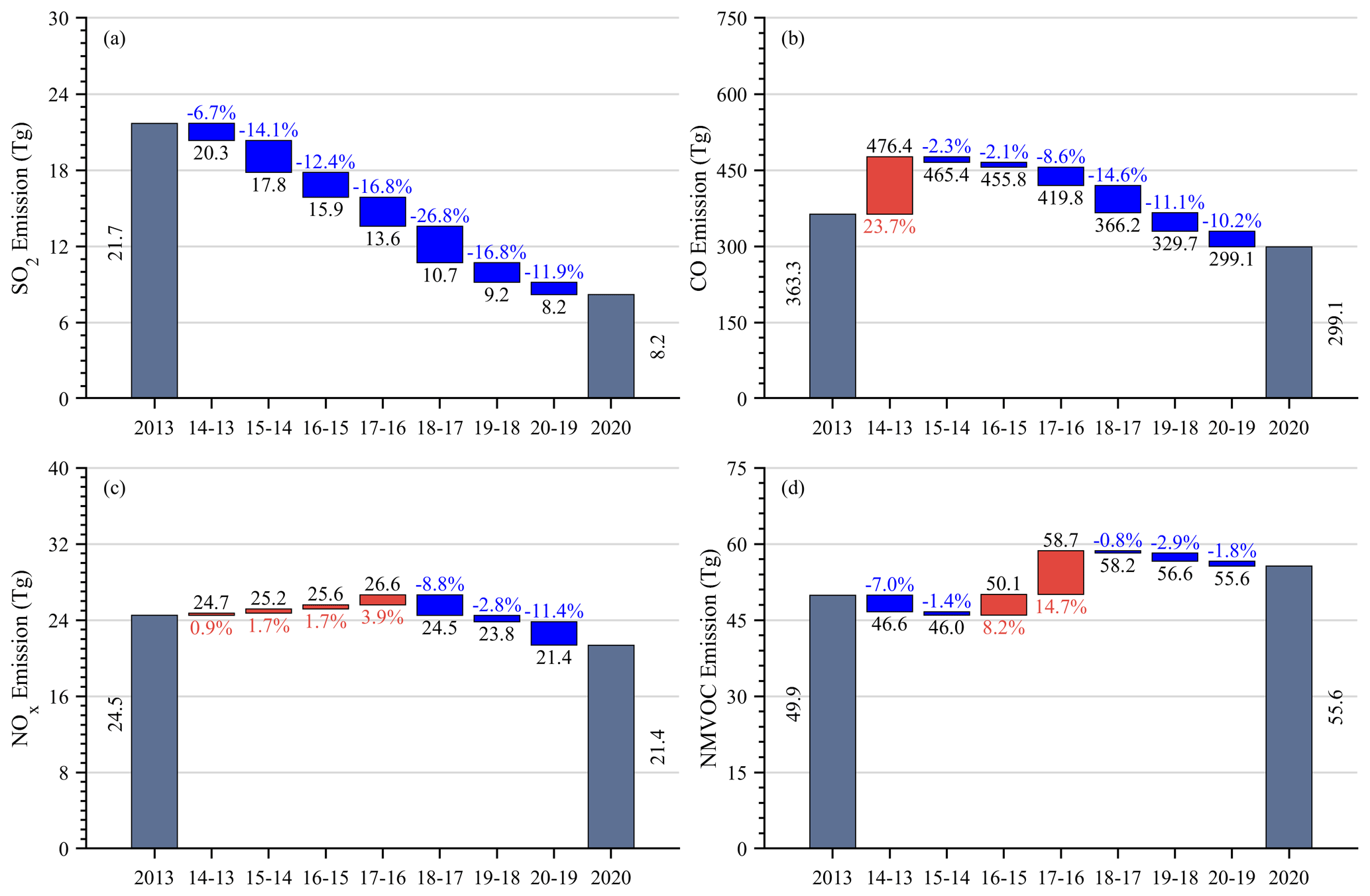
Figure 7 Emission changes in (a) SO₂, (b) CO, (c) NO_x, and (d) NMVOCs obtained from CAQIEI from 2013 to 2020.

4.2.2 Emission changes in gaseous air pollutants

SO₂ and CO

Figure 7 shows the emission changes in different gaseous air pollutants in China from 2013 to 2020. Similar to the PM emissions, SO₂ and CO emissions decreased continuously during the two action plan periods, with top-down estimated emission reductions of approximately 9.6 Tg (54.1 %) and 166.3 Tg (35.7 %) for SO₂ and CO from 2015 to 2020, respectively. Meanwhile, both SO₂ and CO showed a significant decreasing trend from 2015 to 2020, with estimated trends of approximately −2.1 and −36.0 Tg yr⁻¹, respectively (Table 5). The reductions in SO₂ and CO emissions are closely consistent with the strict emission control measures imposed during the action plan periods, such as the phasing-out of outdated industrial capacities and high-emitting factories, the strengthening of emission standards for the industrial and power sectors, the elimination of small coal-fired industrial boilers, and the replacement of coal with cleaner energies, which reflect the effectiveness of the emission control measures during the two action plan periods. Reductions in SO₂ emissions were generally steady during the two action plan periods, which were approximately 4.2 Tg (23.8 %) from 2015 to 2017 and 2.5 Tg (23.5 %) from 2018 to 2020. However, CO showed a different emission reduction rate during the two action plan periods, with its emission reductions (67.1 Tg, 18.3 %) during 2018–2020 being larger than those (45.6 Tg, 9.8 %) during 2015–2017. This contrast may reflect the different emission control policies during the two clean-air action periods as well as the different emission distributions among the sectors between SO₂ and CO. According to the estimates of Zheng et al. (2018), the share of emissions from the industrial and power sectors for SO₂ (77 %) is nearly double that for CO (39 %). Thus, the smaller reduction in CO emissions than that of SO₂ during 2015–2017 provides evidence that the 2013–2017 action plan focused mainly on controlling the emissions from the industrial and power sectors. During the 2018–2020 action plan, strict control measures targeting the residential and transportation sectors were also implemented, which together account for 61 % of CO emissions but only 23 % of SO₂ emissions. As a result, CO showed a larger emission reduction rate during 2018–2020, while the emission reduction rate for SO₂ was similar to that during 2015–2017. The calculated trends of SO₂ and CO emissions during the two action plans are presented in Table 4, which are −2.1 and −1.3 Tg yr⁻¹ for SO₂ and −22.8 and −33.5 Tg yr⁻¹ for CO, respectively.

The reduction in SO₂ and CO emissions was also evident on the regional scale (Figs. S5 and S6 in the Supplement). According to the top-down estimation, the reduction in SO₂ emissions ranged from 0.44 to 2.42 Tg (41.7 %–69.9 %) from 2015 to 2020, with the NCP region exhibiting the largest reductions. The calculated decreasing trend of SO₂ emissions was also significant over all the regions, ranging from −0.08 Tg yr⁻¹ over the NW region to −0.57 Tg yr⁻¹ over the NCP region (Table 5). With regards to the emission reduction rate during the different action plans, the results suggest that the emission reduction rate of SO₂ was higher during 2015–2017 (by 20.8 %–39.8 %) than that during 2018–2020 (by 16.6 %–29.0 %) over the NCP, SE, NE, and SW regions. This may have been because, after the strict emission controls imposed upon industrial and power plants during the 2013–2017 action plan, the room for further reductions in SO₂ emissions became smaller during the 2018–2020 action plan over these regions. Although residential and vehicle emissions were controlled more strictly during the 2018–2020 action plan, in total they account for ∼20 % of anthropogenic SO₂ emissions in China (Zheng et al., 2018). Thus, the enhanced reductions in SO₂ emissions from the residential and transportation sectors may not have been able to fully compensate for the weakened reductions from the industrial and power sectors, leading to a smaller SO₂ emission reduction rate over these regions. In contrast, the SO₂ emission reduction rate during 2018–2020 (31.1 %–34.8 %) was higher than that during 2015–2017 (14.1 %–20.4 %) over the NW and Central regions. This may have been due to the fact that the emission controls over the NW and Central regions were relatively weak during the 2013–2017 action plan (as also evidenced by the emission reduction rates of other species) owing to their less-developed economies. During the 2018–2020 action plan, the emission controls over these two regions were strengthened, which led to their higher emission reduction rates. Accordingly, the enhanced SO₂ emission reduction rates over the NW and Central regions compensated for the weakened reduction rates over the other regions, leading to a steady SO₂ emission reduction rate on the national scale.

The reductions in CO emissions from 2015 to 2020 were approximately 14.9–42.3 Tg (21.6 %–51.4 %) over the different regions of China, with significant decreasing trends ranging from −3.0 to −8.7 Tg yr⁻¹ (Fig. S6 and Table 5). Consistent with the comparisons of national CO emission reduction rates between the two action plans, the emission reduction rates during 2015–2017 (4.4 %–24.6 %) were estimated to be smaller than those during 2018–2020 (12.2 %–24.6 %) over all the different regions, except for the Central region, where the CO emission reduction rates were similar during the two action plans (Fig. S6).

NO_x and NMVOCs

The top-down estimated NO_x and NMVOC emissions showed different changes to the other four species by increasing during 2015–2017 but decreasing during 2018–2020. Specifically, NO_x emissions increased slightly by 5.9 % from 2015 (25.2 Tg) to 2017 (26.6 Tg), with a nonsignificant increasing trend of 0.74 Tg yr⁻¹. Then, NO_x emissions began to decrease in 2018, with a top-down estimated emission reduction and a calculated trend of approximately 3.1 Tg (12.7 %) and −1.6 Tg yr⁻¹, respectively, from 2018 to 2020. NMVOCs showed stronger emission increases than did NO_x, with top-down estimated emission increases of approximately 12.7 Tg (27.6 %) and a calculated emission trend of approximately 6.3 Tg yr⁻¹ from 2015 to 2017. Similarly to NO_x, NMVOC emissions began to decrease after 2018, with a top-down estimated reduction of approximately 2.6 Tg (−4.4 %) from 2018 to 2020 and a calculated trend of approximately −1.3 Tg yr⁻¹.

The increases in NO_x and NMVOC emissions during 2015–2017 suggest that the 2013–2017 action plan may not have achieved desirable mitigation effects on these two species. For NO_x emissions, the upward trend may have been associated with the following factors. On the one hand, vehicle exhaust is one of the most important sources of NO_x in China, accounting for 31 % of all NO_x emissions nationally (Zheng et al., 2018). From 2013 to 2017, the number of vehicles in China continued to increase and reached 310 million in 2017, approximately 33.5 % higher than in 2013 (MEE, 2018), which led to increases in NO_x emissions from vehicles in China. On the other hand, although the 2013–2017 action plan was effective in reducing the NO_x emissions from coal-fired power plants by promoting denitrification facilities and an ultra-low emission standard, the mitigation impacts on industrial NO_x emissions may have been relatively small. For example, X. Y. Wang et al. (2019) compiled a unit-based emission inventory for China's iron and steel industry from 2010 to 2015, based on detailed survey results of approximately 4900 production facilities in mainland China. They found that there were almost no NO_x control measures in China's iron and steel industry during 2010–2015, resulting in a 12.4 % increase in China's NO_x emissions from the iron and steel industry in 2015 compared to 2010. In addition, although the penetration rate of denitrification facilities in China's cement industry reached 92 % in 2015, the actual operating rate of denitrification facilities in the cement industry was not desirable, due to the lack of online emission monitoring systems. According to the research results of the Ministry of Ecology and Environment, 800, 1300, and 1400 cement production kilns were equipped with selective non-catalytic denitrification facilities from 2013 to 2015, but the actual operating rates were only 51 %, 54 %, and 73 %, respectively (Liu et al., 2021). In addition, the new precalciner kilns used in the cement industry have a higher NO_x emission factor, such that the shift from traditional vertical kilns to precalciner kilns has to some extent increased the cement industry's emissions of NO_x (Liu et al., 2021). Thus, there is evidence that the mitigation effects of the industrial control measures on NO_x emissions may not be as significant as expected. Overall, the increased number of vehicles may have offset the emission mitigation effects brought about by the control of power plants, and the mitigation effects of controlling industrial NO_x emissions were also undesirable. Consequently, NO_x emissions in China may not have decreased and may even have increased slightly during the 2013–2017 action plan. Figure S7 in the Supplement further shows the changes in NO_x emissions over the different regions of China, revealing that NO_x emissions over the NCP, SE, NE, and SW regions were roughly unchanged (by less than 5 %) from 2015 to 2017, while they increased over the NW (18.6 %) and Central (17.5 %) regions. This is consistent with previous results and indicates that NO_x emissions may have increased over the NW and Central regions, possibly due to their increased human activities and weak emission controls.

In terms of NMVOC emissions, since the inversion results did not differentiate between anthropogenic and biogenic sources, the changes in NMVOC emissions may have been related to both anthropogenic and biogenic emissions. With respect to anthropogenic emissions, previous bottom-up studies suggested that China's NMVOC emissions did not decline during the 2013–2017 action plan due to the lack of effective control measures on the chemical industry and solvent use (Zheng et al., 2018; M. Li et al., 2019). According to the estimates of M. Li et al. (2019), China's NMVOC emissions from solvent use increased by 11.1 % in 2017 compared to those in 2015. Meanwhile, the increase in the number of vehicles in China may also have led to an increase in NMVOC emissions from transportation. Thus, the increases in NMVOC emissions during 2015–2017 estimated by our inversion inventory may be related to the increases in anthropogenic NMVOC emissions from the chemical industry, solvent use, and vehicles. For the trends of biogenic NMVOC emissions, the Copernicus Atmosphere Monitoring Service (CAMS) global emission inventory shows that there were only little changes in the biogenic NMVOC emissions in China from 2013 to 2018 (Sect. 4.3.3), suggesting little contributions of the biogenic sources to the increased NMVOC emissions in China. Figure S8 in the Supplement further shows the changes in NMVOC emissions over the different regions of China, which suggests consistent increases in NMVOC emissions from 2015 to 2017 over the different regions. According to the top-down estimations, NMVOC emissions increased by 30.5 %, 25.2 %, 18.5 %, 10.9 %, 50.5 %, and 63.1 % over the NCP, SE, NE, SW, NW, and Central regions, respectively. Again, the NW and Central regions exhibited the largest emission increases among the six regions, which is consistent with their elevated levels of human activity and weak emission controls.

The decrease in NO_x and NMVOC emissions after 2018 suggests that the emission control strategy of the Chinese government had reached a point of optimization. The 2018–2020 action plan strengthened not only the controls on the industrial and power sectors, but also the transportation sector, especially for diesel vehicles with high NO_x emissions. For example, the Chinese government released the Action Plan for the Control of Diesel Trucks and vigorously promoted an adjustment of the transportation structure of China by gradually improving the availability of rail transport. As a result, there was a downward trend in NO_x emissions in China. The top-down estimated reductions in NO_x emissions were approximately 0.81 Tg (17.2 %) over NCP, 0.98 Tg (14.0 %) over SE, 0.37 Tg (9.4 %) over NE, 0.51 Tg (12.2 %) over SW, 0.13 Tg (11.0 %) over NW, and 0.32 Tg (9.2 %) over the Central region (Fig. S7). The decrease in NMVOC emissions after 2018 may on the one hand have been related to the strengthening of vehicle controls during the 2018–2020 action plan, while on the other hand it may have been related to the promotion of clean heating plans in the northern China region, which reduced the emissions of NMVOCs from residential sources. However, the decreases in NMVOC emissions were smaller than those of NO_x, which were estimated to be 0.84 Tg (6.9 %) over NCP, 0.47 Tg (2.8 %) over SE, 0.98 Tg (10.1 %) over NE, and 0.53 Tg (14.1 %) over NW (Fig. S6). Different from other regions, the NMVOC emissions over the SW and Central regions remained almost unchanged during the 2018–2020 action plan (Fig. S8).

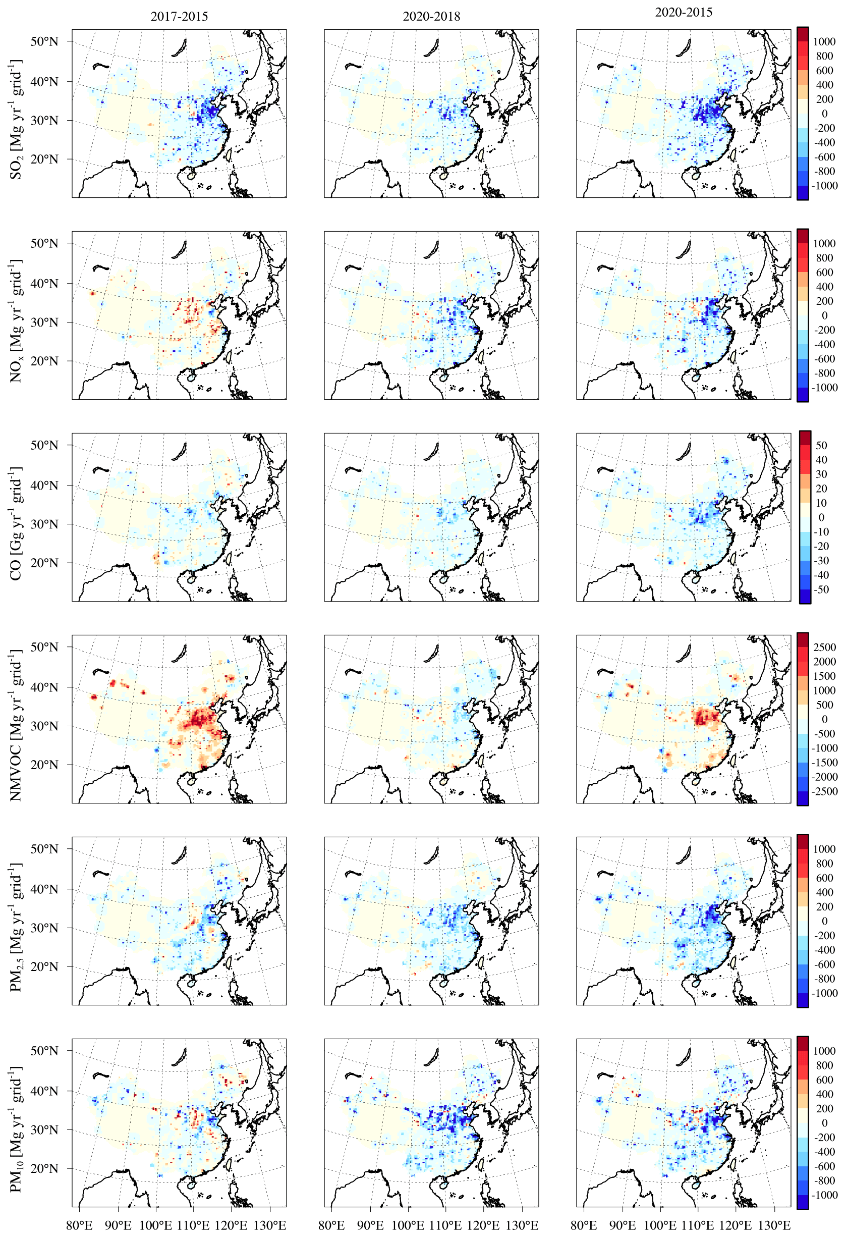
Figure 8 Spatial distributions of the emission changes in different species during 2015–2017 (left panels), 2018–2020 (middle panels), and 2015–2020 (right panels) obtained from CAQIEI from 2013 to 2020.

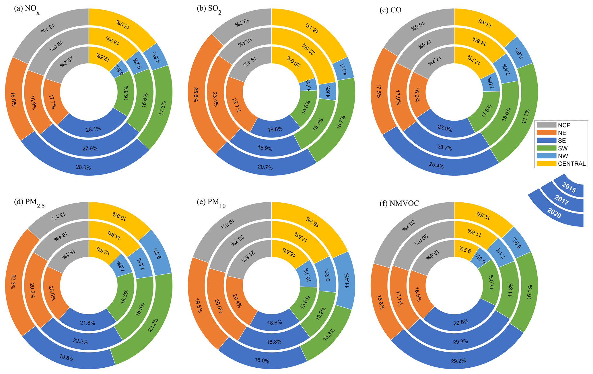
Figure 9 Emission distributions of (a) NO_x, (b) SO₂, (c) CO, (d) PM_2.5, (e) PM₁₀, and (f) NMVOCs among the different regions in China obtained from CAQIEI in 2015, 2017, and 2020.

4.2.3 Changes in the distribution pattern of emissions in China

Due to the different emission control intensities over the different regions of China, the emission distribution patterns of the different species may also have been altered, which could have influenced the distributions of air pollution in China. Based on CAQIEI, we further investigated the emission distribution patterns, as well as their changes, during the two action plans. Maps of the emission changes in different species during 2015–2017 and 2018–2020 are presented in Fig. 8. The shares of emissions in 2015, 2017, and 2020 for each subregion of China are also presented (Fig. 9). It can be seen that the emission changes during 2015–2017 were more heterogenous than those during 2018–2020. The air pollutant emissions after the 2018–2020 action plan showed consistent reductions over most regions of China, while there were obvious emission increases detected from 2015 to 2017. This is consistent with the different emission control effects during the two clean-air action plans, as mentioned in the previous sections. Due to its strict emission control policies, the NCP region showed consistent emission reductions in SO₂, NO_x, CO, PM_2.5, and PM₁₀ during the two clean-air action plans. Accordingly, the shares of emissions in the NCP region continued to decrease during the two action plan periods (Fig. 9). For example, the share of SO₂ emissions in the NCP region decreased from 19.4 % to 15.4 % during the period of 2015–2017 and from 15.4 % to 12.7 % during the 2018–2020 action plan. In contrast, NMVOC emissions increased obviously over the NCP region from 2015 to 2017 and decreased from 2018 to 2020. However, the share did not change significantly, being roughly 20 % throughout both periods. As for the other regions, increases in SO₂, NO_x, PM_2.5, PM₁₀, and NMVOC emissions during 2015–2017 could be found over the Central region. More specifically, the emission increases were mainly located in the Fenwei Plain area of central China, which was due to the fact that this area was not included as a key region of emission controls during the 2013–2017 action plan. However, the Fenwei Plain area was added as a key emission control region during the 2018–2020 action plan, which is consistent with the emission reductions for these species over the Central region (Fig. 8). As a result, the shares of SO₂ and PM_2.5 emissions in the Central region increased during 2015–2017 but decreased during 2018–2020 (Fig. 9). However, the shares of NO_x, PM₁₀, and NMVOC emissions continued to increase over central China during the two clean-air action plans, which suggests larger roles of air pollutant emissions in that region. In contrast, the share of CO emissions in central China continued to decrease in the two action plans, from 17.7 % in 2015 to 13.4 % in 2020.

In terms of the shares of emissions in eastern and western China, the top-down estimation suggests increased shares of NO_x, PM_2.5, PM₁₀, and NMVOC emissions in western China after the two clean-air action plans (Fig. 9), which indicates slower emission reductions for these species in western China. However, the share of CO emissions in western China was reduced after the two clean-air action plans. Although the share of SO₂ emissions in western China increased during 2015–2017, this turned to a decrease during 2018–2020.

4.3 Comparisons with different emission inventories

In this section, CAQIEI is compared with the previous long-term bottom-up and top-down emission inventories in China to validate our inversion results and provide the clues for the potential uncertainty in the current air pollutant emission inventories. The bottom-up emission inventories used in the comparison include MEIC (Zheng et al., 2018), ABaCAS (Li et al., 2023), HTAPv3 (Crippa et al., 2023), EDGARv6 (Jalkanen et al., 2012), and CEDS (McDuffie et al., 2020), while the top-down emission inventory is obtained from the updated Tropospheric Chemistry Reanalysis (TCR-2) (Miyazaki et al., 2020a). However, it is difficult to directly compare our inversion results with these emission inventories considering that the inversed emission includes both anthropogenic and natural emissions. To better compare our inversion results with previous inventories, the natural emission sources, including soil NO_x emissions and biogenic emissions obtained from the CAMS global emission inventory (https://ads.atmosphere.copernicus.eu/cdsapp#!/dataset/cams-global-emission-inventories?tab=overview; last access: 26 July 2023) and the biomass burning emissions obtained from the Global Fire Assimilation System (GFAS) (Kaiser et al., 2012), are taken as a reference to account for the influences of natural sources. The CAMS and GFAS emission inventories are used because they are state-of-the-art natural emission inventories and can provide us with independent long-term estimations of natural emissions. Since the latest year of most emission inventories is 2018, the comparisons were conducted between 2015 and 2018. Note that, due to the complexity of the estimations of natural sources, significant uncertainty exists in the estimated natural emissions. As a result, the comparison results would be sensitive to the used natural emission inventories, especially for the species with a large amount of natural emission, such as the NMVOCs and particulate matter. Therefore, one should be aware of the comparison conducted here and the derived implications on the basis of the natural emissions estimated by CAMS and GFAS. In addition, the natural dust emissions are not considered in the comparisons, which would influence the comparisons of the PM emissions.

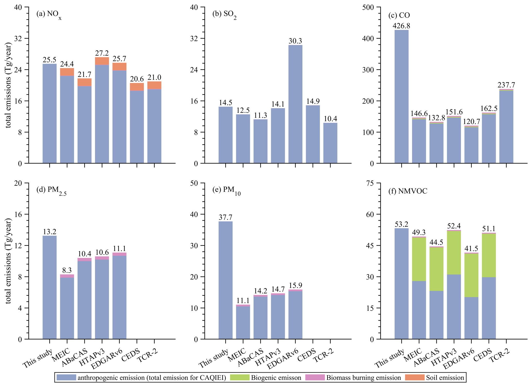
Figure 10 Comparisons of the averaged emissions of (a) NO_x, (b) SO₂, (c) CO, (d) PM_2.5, (e) PM₁₀, and (f) NMVOCs over China from 2015 to 2018 between CAQIEI and previous inventories added with natural sources.

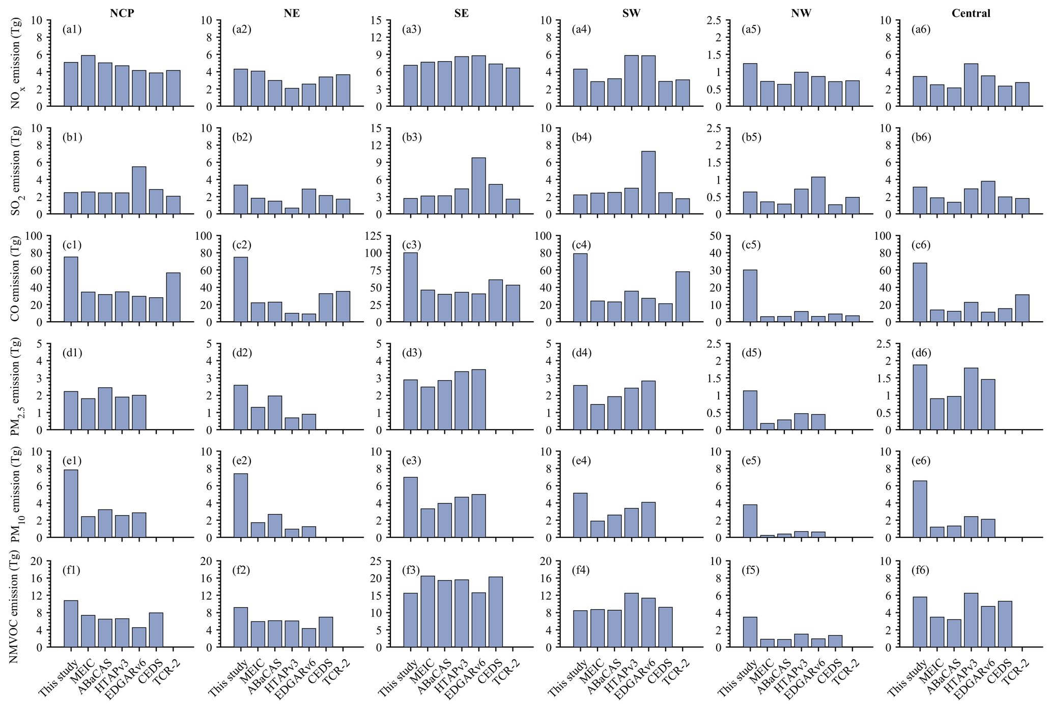
Figure 11 Comparisons of the averaged emissions of (a) NO_x, (b) SO₂, (c) CO, (d) PM_2.5, (e) PM₁₀, and (f) NMVOCs over the different regions in China from 2015 to 2018 between CAQIEI and previous inventories added with natural sources.

4.3.1 Magnitude

NO_x

Figure 10 shows the average emissions of different air pollutants in China during 2015–2018 obtained from CAQIEI and the previous emission inventories plus the natural sources we considered. Comparisons of the emission estimations on the regional scale and gridded scale are also presented (Fig. 11 and Fig. S9 in the Supplement). The results show that CAQIEI has slightly higher NO_x emissions in China than the other inventories. Considering that CAQIEI includes both anthropogenic and natural sources, this discrepancy could be explained by the natural NO_x sources. According to the estimations of CAMS and GFAS, the soil and biomass burning NO_x emissions are approximately 1.9 and 0.08 Tg yr⁻¹, which explains the higher NO_x emissions given by CAQIEI well. After consideration of the natural sources, MEIC, HTAPv3, and EDGARv6 agree well with our inversion results on the national scale, with their differences being within 1.0 %–7.4 %. The NO_x emissions estimated by ABaCAS, CEDS, and TCR-2 are slightly lower than CAQIEI and other emission inventories. However, the differences between CAQIEI and these inventories were found to range from 15.9 % to 21.3 %, which is within the previous estimated uncertainties of NO_x emissions in China (Kurokawa and Ohara, 2020; M. Li et al., 2017; S. Li et al., 2023). These results suggest that the total NO_x emissions in CAQIEI are generally consistent with the current estimations of the anthropogenic and natural NO_x emissions in China. On the regional scale, the top-down estimated NO_x emissions show good agreement with the previous emission inventories over the NCP and SE regions, with their differences ranging from 1.0 % to 26.8 %, suggesting good consistency in the estimations of NO_x emissions over these two regions. This makes sense because NCP and SE are the two most developed regions in China, where surveys and research on emissions are the most sufficient. The differences are larger over the other regions. In the NE region, CAQIEI has higher NO_x emissions than the other inventories by 5 %–70 %, suggesting higher anthropogenic or biomass burning emissions over there. The estimations made by MEIC, CEDS, and TRC-2 are closer to our estimates, with their differences being approximately 5.4 %–23.3 %, while the differences are larger for ABaCAS, HTAPv3, and EDGARv6 (36.7 %–70.0 %). Over the SW and Central regions, there are large diversities in the previous emission inventories, with estimations by HTAPv3 and EDGARv6 almost double those of MEIC, ABaCAS, CEDS, and TCR-2. CAQIEI suggests a middle estimation which is within the range of previous emission inventories. In the NW region, CAQIEI is consistently higher than other inventories, by 22.7 %–64.2 %, which suggests a potential missing source of the NO_x emissions over this region.

SO₂

For SO₂ emissions, since natural sources contribute little (only about 0.02 Tg yr⁻¹) to them in China, the discrepancies between CAQIEI and previous emission inventories are mainly attributable to the differences in anthropogenic emissions. As shown in Fig. 10, CAQIEI agrees well with HTAPv3 and CEDS on the national scale, with their differences being approximately ±2 %, but it is higher than MEIC, ABaCAS, and TCR-2 by 17.4 %–32.9 %. In contrast, EDGARv6 may have a positive bias in its estimated SO₂ emissions, which are roughly double those of CAQIEI and other inventories. On the regional scale, our results agree well with MEIC, ABaCAS, HTAPv3, CEDS, and TCR-2 over the NCP region, with their differences ranging from 1.0 to 18.1 %. In the SE region, CAQIEI suggests lower SO₂ emissions than previous emission inventories, except for TCR-2. The differences are relatively smaller for the MEIC and ABaCAS inventories by around −15 % but are larger for HTAPv3, EDGARv6, and CEDS (ranging from −47.3 % to −113.2 %). In contrast, CAQIEI suggests higher SO₂ emissions than all previous emission inventories over the NE region by about 14.8 %–132.0 %, indicating possible missing sources over there. Similarly, CAQIEI and HTAPv3 suggest higher SO₂ emissions than MEIC, ABaCAS, CEDS, and TCR-2 by 27.0 %–75.6 % in the NW region and by 44.3 %–77.7 % in the Central region.

Table 6 The top-down estimated CO emissions in China from the previous inventories.

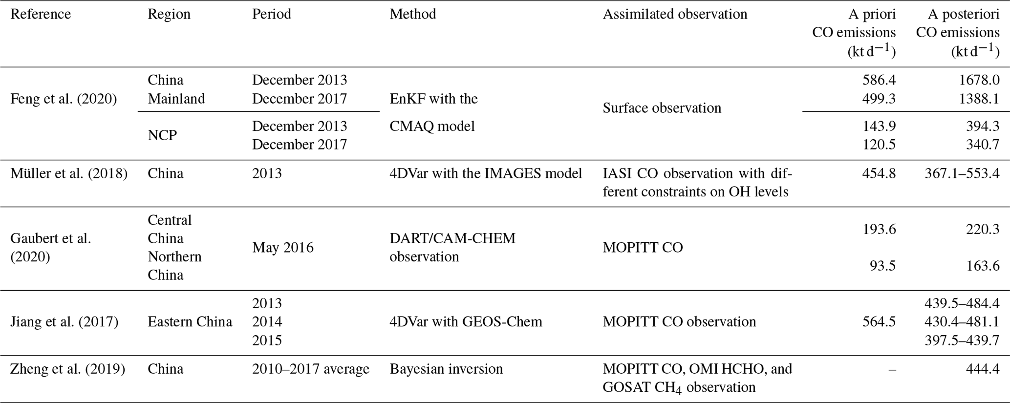
CO

For CO emissions, CAQIEI is substantially higher than the previous emission inventories, with the estimated CO emissions of CAQIEI being about 3 times higher than the bottom-up inventories and more than 2 times the top-down estimates made by TCR-2. According to GFAS, the average rate of CO biomass burning emissions in China from 2015 to 2018 was about 3.4 Tg yr⁻¹. Yin et al. (2019), based on MODIS fire radiative energy data, also estimated China's CO biomass burning emissions to be about 5.0 (2.3–7.8) Tg yr⁻¹. The biogenic CO emissions obtained from the CAMS global emission inventory were approximately 2.3 Tg yr⁻¹. According to these estimates, natural CO emissions in China have a magnitude of approximately 10, which is rather small compared with the anthropogenic sources and cannot explain the large discrepancies between CAQIEI and other inventories. Thus, CAQIEI suggests much higher anthropogenic CO emissions in China than in the existing emission inventories. In fact, the potential underestimation of CO anthropogenic emissions has been investigated in previous studies and is regarded as the main reason for the negative bias in global or hemispheric CO simulations (Stein et al., 2014; Gaubert et al., 2020). Regionally, Kong et al. (2020) compared a suite of 13 modeling results from six different CTMs – i.e., NAQPMS, CMAQ, WRF-Chem, NU-WRF, NHM-Chem, and GEOS-Chem – with observations over the NCP and Pearl River Delta regions in the framework of the Model Inter-Comparison Study for Asia III (MICS-Asia III) and found consistent negative biases in the CO simulations of all the models, pointing toward potential underestimations of CO emissions in China. Previous inversion studies have also reported higher a posteriori CO emissions than their a priori emission inventories (Bergamaschi et al., 2000; Miyazaki et al., 2012; Petron et al., 2002, 2004; Tang et al., 2013; Gaubert et al., 2020). For example, the constrained CO emissions reported by Gaubert et al. (2020) are 80 % higher than the CEDS over northern China. Our inversion results are consistent with these inversion studies, suggesting higher anthropogenic CO emissions in China. However, direct evidence in support of such high CO emissions in China reported by our study is still limited currently. Thus, we compiled more inversion results in the period 2013–2020 from previous studies to further validate our inversion results, which are summarized in Table 6. It can be seen clearly that there are large differences in the estimated CO emissions between the inversion results based on surface observations and those based on satellite data. Our inversion results are consistent with the results of Feng et al. (2020), with China's CO emissions in December 2017 estimated at approximately 1500.0 and 1388.1 kt d⁻¹, respectively. In addition, Feng et al. (2020) used the CMAQ model to constrain CO emissions, which is different from the model we used. This may indicate that the model uncertainty would not significantly influence the inversion results of CO emissions. However, the top-down estimated CO emissions based on satellite data (163.6–553.4 kt d⁻¹) are much lower than those based on surface observations, although they are all higher than their a priori emissions. The lower CO emission estimations based on satellite data assimilation may be attributable to the lower sensitivities of satellite data to surface concentrations, suggesting that the assimilation of satellite data alone may not be adequate for correcting the negative biases in the a priori emissions. This deficiency was also shown by Miyazaki et al. (2020a), who found undercorrected surface CO emissions in the extratropics of the Northern Hemisphere in TCR-2. However, the assimilation of surface observations can be influenced by the uncertainties in the modeled vertical mixing, which could lead to the uncertainties in the inversed CO emissions based on surface observations. Therefore, the inversed CO emissions in CAQIEI could be partly supported by previous inversion studies based on surface observations, but more evidence is still needed to justify the magnitude of the inversed CO emissions. Besides anthropogenic sources, the chemical production of CO via oxidation of methane (CH₄) and NMVOCs, together with the CO sinks via the hydroxyl radical (OH) reaction, also influences the simulation of CO (Stein et al., 2014; Gaubert et al., 2020; Müller et al., 2018). Due to the important role of OH in the chemical production and sinks of CO, the inversion of CO emissions is sensitive to the modeled OH abundance and the emissions of CH₄ and NMVOCs. According to the estimation of Müller et al. (2018), the magnitude of inversed CO emissions in China could differ by more than 40 % when different levels of OH concentrations are used in the model. Thus, the much higher estimations of CO emissions in our inversion results may also be partly explained by the underestimation of CO chemical production or the overestimation of the CO sink.

PM_2.5

In terms of PM_2.5, CAQIEI suggests higher emissions than ABaCAS, HTAPv3, and EDGARv6 of about 20 % and 47.7 % higher emissions than MEIC on the national scale. Larger discrepancies mainly occur in the NE and NW regions, where CAQIEI is about 27.2 %–114.9 % and 83.2 %–143.2 % higher than in the previous inventories. The differences in the estimated PM_2.5 emissions may be related to the uncertainties in the biomass burning or anthropogenic sources in the NE region (J. Wu et al., 2020), while in the NW region the errors in the fine-dust emissions may also contribute to the differences in the estimated PM_2.5 emissions there. The differences in the estimated PM_2.5 emissions are relatively smaller in the NCP and SE regions, ranging from −18.9 % to 20.4 %, suggesting better agreement in the estimated PM_2.5 emissions over these two regions. In the SW region, CAQIEI is closer to HTAPv3 and EDGARv6, with their differences being about 6.3 % and −9.5 %, respectively, which is higher than MEIC and ABaCAS by 54.2 % and 28.6 %, suggesting higher uncertainty in the estimated PM_2.5 emissions over there.

PM₁₀

For PM₁₀ emissions, it is difficult to directly compare CAQIEI with previous emission inventories since CAQIEI contains not only anthropogenic and biomass burning emissions, but also coarse-dust emissions. As a result, the estimated emissions of PM₁₀ by CAQIEI are substantially higher than those of previous inventories, especially over the NW, Central, and NE regions (Fig. 11), which are the typical natural windblown dust source regions in China (Zeng et al., 2020). Besides the naturally windblown dust of arid desert regions (Prospero et al., 2002), large amounts of coarse-dust emissions also stem from anthropogenic sources, including anthropogenic fugitive, combustion, and industrial dust (AFCID) from urban sources (Philip et al., 2017) and anthropogenic windblown dust from human-disturbed soils due to changes in land use practices, deforestation, and agriculture (Tegen et al., 1996). Therefore, although the other regions are not typical natural windblown dust source regions in China, there are still high levels of coarse-dust emissions from anthropogenic sources there (also called “urban dust”), which may be the main reason for the large deviation in the estimated PM₁₀ emissions between CAQIEI and the previous inventories. On the one hand, although AFCID is included in MEIC, ABaCAS, HTAPv3, and EDGARv6, it is difficult for current bottom-up emission inventories to completely represent fugitive sources (Philip et al., 2017). On the other hand, the anthropogenic windblown dust emissions have not been included in current bottom-up emission inventories, which is an important source of coarse dust in urban areas according to the estimations of Li et al. (2016) and is another important contributor to the differences between CAQIEI and previous emission inventories.

NMVOCs

For NMVOC emissions, since CAQIEI includes both anthropogenic and natural sources, its estimated NMVOC emissions are much higher than those estimated by previous emission inventories. After consideration of natural sources, CAQIEI suggests close estimations of the NMVOC emissions with the MEIC, HTAPv3, and CEDS inventories on the national scale, with their differences being about 1.5 %–12.5 %. The estimated NMVOC emissions by ABaCAS and EDGARv6 are slightly lower than CAQIEI by 17.8 % and 24.6 %, respectively. On the regional scale, CAQIEI suggests higher NMVOC emissions over northern China (NCP, NE, and NW), with the top-down estimated NMVOC emissions of about 30.4 %–81.4 %, 27.3 %–72.1 %, 79.3 %–116.8 %, and 8.7 %–57.5 % being higher than those of the previous emission inventories. In contrast, CAQIEI suggests lower NMVOC emissions over the SE region, with the estimated NMVOC emissions of CAQIEI being about 21.2 %–27.6 % lower than those of MEIC, ABaCAS, HTAPv3, and CEDS. These results are consistent with the previous inversion results based on the satellite observations, which suggest higher NMVOC emissions over the NCP region and lower NMVOC emissions over southern China (Souri et al., 2020). Over the SW region, CAQIEI shows good agreement with MEIC, ABaCAS, and CEDS, with CAQIEI being slightly lower than these inventories by 1.0 %–8.9 %, but it is lower than HTAPv3 and EDGARv6 by about 38.6 % and 29.1 %, respectively. Again, it should be noted that the comparisons of NMVOC emissions are conducted on the basis of natural emissions estimated by CAMS and GFAS and could be more sensitive to the used natural sources than other species considering the larger contributions of the natural source to the NMVOC emissions.

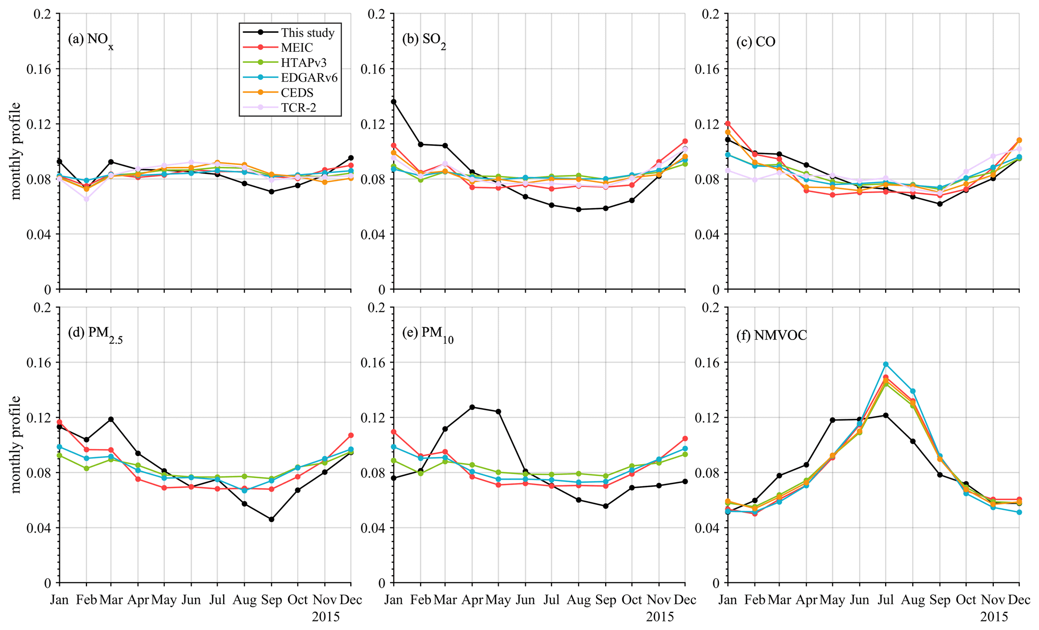
Figure 12 Comparisons of the monthly profiles of (a) NO_x, (b) SO₂, (c) CO, (d) PM_2.5, (e) PM₁₀, and (f) NMVOCs over China averaged from 2015 to 2018 between CAQIEI and previous inventories added with natural sources.

4.3.2 Seasonality

Figure 12 presents the monthly profiles of different air pollutants obtained from different emission inventories. Note that the natural sources have been added to the previous inventories to facilitate the comparisons. The results show that different emission inventories give similar monthly profiles of NO_x and CO emissions, with higher emissions during wintertime and lower emissions during summertime, which suggests relatively lower uncertainty in the estimated monthly profiles for these two species. For SO₂ emissions, CAQIEI yields a stronger monthly variation than the other inventories, with a higher proportion from January to March and a lower proportion during summertime. Due to the influences of dust emissions, the top-down estimated PM_2.5 and PM₁₀ emissions show higher proportions than the other emission inventories during the spring season, especially for PM₁₀. However, the proportions of emissions during fall and winter are lower than in the other inventories. The monthly profiles of NMVOC emissions are generally consistent, with higher emissions during summer due to the enhanced biogenic emissions. However, the profile of CAQIEI is flatter than the previous inventories and suggests a higher proportion during springtime. In addition, the timings of peak values of NMVOC emissions are also different between CAQIEI and the previous inventories, with CAQIEI showing peak values during May–July but the other inventories suggesting peaks during June–August.

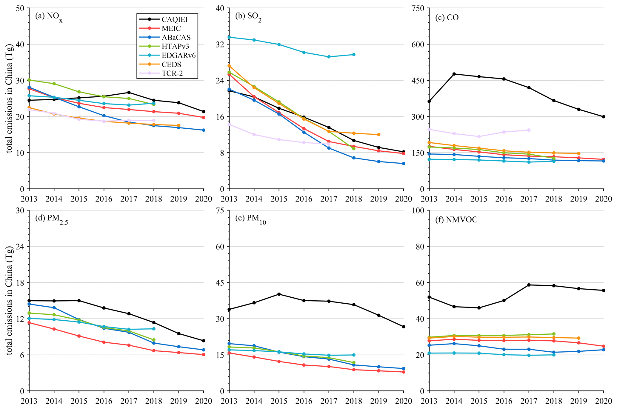
Figure 13 Time series of annual emissions of (a) NO_x, (b) SO₂, (c) CO, (d) PM_2.5, (e) PM₁₀, and (f) NMVOCs over China from 2013 to 2020 obtained from CAQIEI and previous inventories. Note that the natural sources were not included in the previous inventories in this figure.

4.3.3 Emission changes during 2015–2018

The top-down estimated emission changes in different air pollutants during 2015–2018 were also compared with previous emission inventories. Figure 13 shows the time series of the total emissions of different species from 2013 to 2020 obtained from CAQIEI and other emission inventories. Comparisons of the emission changes over the regional scales are also presented in Figs. S10–S15 in the Supplement. Before the comparison, we first analyze the trends of natural sources in China to investigate their influences on the emission changes in different species based on the CAMS emission inventory and GFAS. Note that we only consider the soil, biogenic, and biomass burning emissions for the natural sources; the trends of dust emissions in China are not analyzed, which may lead to uncertainty when comparing the emission changes in PM_2.5 and PM₁₀. As shown in Fig. S16 in the Supplement, the natural sources of NO_x and NMVOC emissions changed little during 2013–2018. The other species had small decreasing trends from 2013 to 2018. However, considering the small contributions of natural sources to their emissions, these small trends would not significantly influence their emission trends. For the dust emissions, previous studies have indicated a declining trend in dust activity in China from 2001 to 2020 (Wu et al., 2022; Wang et al., 2021) due to weakened surface wind and increased vegetation cover and soil moisture. These results suggest that the emission trends in CAQIEI would mainly be driven by the anthropogenic sources of the gaseous air pollutants based on the estimations of CAMS and GFAS, while its estimated emission trends of PM_2.5 and PM₁₀ would be influenced by the declining trends in dust emissions in China, which should be noted when comparing the emission changes in PM_2.5 and PM₁₀.

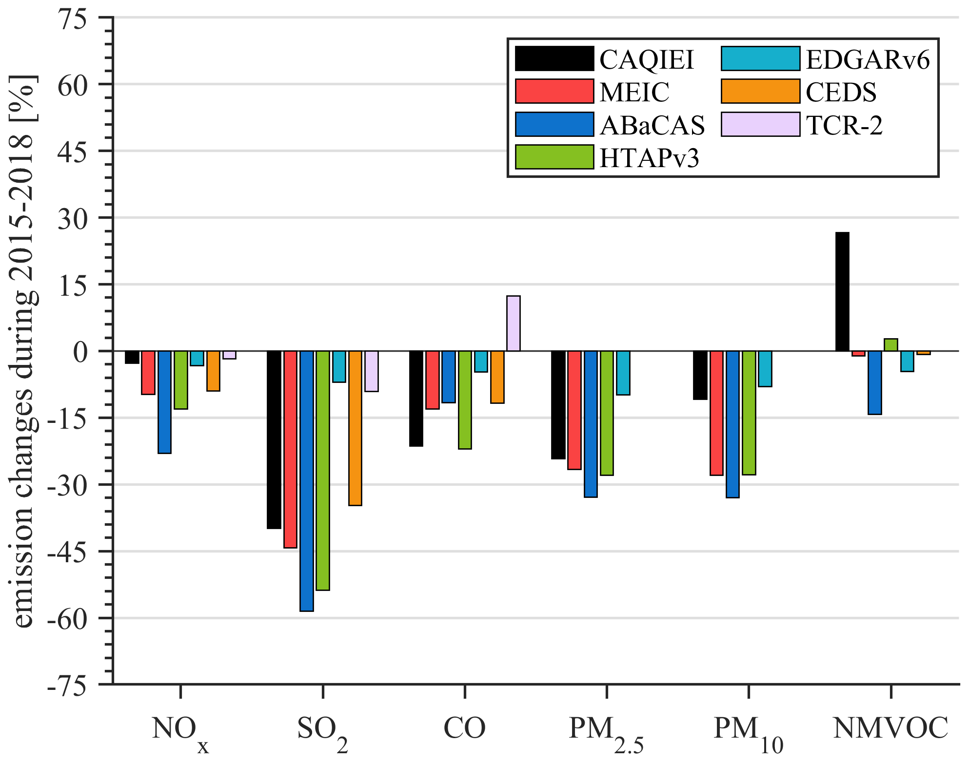
Figure 14 Comparisons of the calculated emission changes in NO_x, SO₂, CO, PM_2.5, PM₁₀, and NMVOCs over China from 2015 to 2018 between CAQIEI and previous inventories. Note that the natural sources were not included in the calculation of the emission changes in this figure.

As shown in Fig. 14, all the emission inventories agree that the NO_x, SO₂, CO, PM_2.5, and PM₁₀ emissions in China were reduced from 2015 to 2018, except for the increases in CO emissions estimated by TCR-2, which confirms the effectiveness of the emission control policies implemented during the clean-air action plans. Meanwhile, most emission inventories agree that SO₂ is the species with the largest emission reduction rate, followed by PM_2.5, indicating better emission mitigation effects of these two species (Fig. 14). However, CAQIEI suggested lower emission reduction rates than the other emission inventories for most of the species, especially for NO_x, PM₁₀, and NMVOCs (Fig. 14). The estimated emission reduction rate of NO_x obtained from CAQIEI is about −2.7 %, which is lower than the values of MEIC (−9.7 %), ABaCAS (−23.0 %), HTAPv3 (−13.0 %), and CEDS (−9.0 %). As we discussed in Sect. 4.2.2, “NO_x and NMVOCs”, the small reductions in NO_x emissions in CAQIEI would be related to the increased vehicle emissions and the undesirable mitigation effects of the industry control. In fact, these factors have been considered in some bottom-up emission inventories, such as MEIC. The differences between our inversion results and previous inventories thus reflect uncertainty in the quantifications of the effects of these factors on the NO_x emissions due to the lack of sufficient statistics on the mobile vehicle sector or other sectors. Our inversion results suggest larger adverse effects of these two factors on the reductions in NO_x emissions in China. According to Fig. S17 in the Supplement, the differences between CAQIEI and these inventories mainly occur in the SE, SW, NW, and Central regions, with the emission reduction rate estimated by CAQIEI being substantially lower than those estimated by previous inventories. In particular, CAQIEI suggests increases in NO_x emissions over the Central region, which is contrary to the previous emission inventories. Better agreement is achieved over the NCP and NE regions, with the emission reduction rate estimated by CAQIEI being closer to those of MEIC, HTAPv3, and CEDS. The NO_x emission reduction rates estimated by EDGARv6 (−3.3 %) and TCR-2 (−1.7 %) are closer to our results on the national scale, but they estimated a lower NO_x emission reduction rate than our estimate over the NCP and NE regions.

Similarly, the emission reduction rate of PM₁₀ obtained from CAQIEI (−10.8 %) is lower than those estimated by MEIC (−27.9 %), ABaCAS (−33.0 %), and HTAPv3 (−27.8 %) on the national scale (Fig. 14). A lower PM₁₀ emission reduction rate of CAQIEI than these inventories also exists in the different regions of China, except SW (Fig. S17). In particular, and different from previous emission inventories, CAQIEI suggests that PM₁₀ emissions may have actually increased over the Central region. Considering that dust emissions may have decreased from 2015 to 2018 owing to weakened dust events (Wang et al., 2021), the increase in PM₁₀ emissions over the Central region may reflect the increases in anthropogenic sources. Meanwhile, we also found that CAQIEI estimated the emission reduction rate of PM₁₀ to be smaller than that of PM_2.5. This is different from previous emission inventories, which show similar emission reduction rates for PM_2.5 and PM₁₀. Considering that PM₁₀ emissions include PM_2.5 and PMC emissions, the lower emission reduction rate of PM₁₀ than PM_2.5 in CAQIEI suggests that PMC emissions may have decreased more slowly than PM_2.5 emissions from 2015 to 2018.

In terms of NMVOCs, most previous inventories, including MEIC, EDGARv6, and CEDS, suggest a weak decrease in China, with the estimated rates of change in emissions ranging from −0.8 % to −4.6 %. The emission reduction rate estimated by ABaCAS is larger, reaching up to −14.2 %. In contrast, CAQIEI suggests an opposite emission change to these inventories, with the estimated NMVOC emissions increasing by 26.6 % from 2015 to 2018. HATPv3 also suggests an increase in NMVOC emissions but with a much lower rate of increase (2.7 %). Similar results were also found on the regional scale (Fig. S17), especially over the NCP, NE, and Central regions, where NMVOC emissions could have increased by 38.0 %, 38.3 %, and 60.0 %, respectively, according to the estimates of CAQIEI. As we discussed in Sect. 4.2.2, “NO_x and NMVOCs”, the increases in NMVOC emissions estimated in CAQIEI may be related to the increased anthropogenic NMVOC emissions from the chemical industry, solvent use, and vehicles. Therefore, similar to the NO_x emissions, the differences between CAQIEI and the previous inventories reflect the uncertainty in the quantifications of the impacts of these factors and suggest larger adverse effects of these factors on the emission reductions in NMVOC emissions than the previous inventories.

The differences in the estimated emission reduction rates between CAQIEI and previous inventories are relatively smaller for SO₂ and PM_2.5 emissions. The emission reduction rate of SO₂ estimated by CAQIEI is close to that estimated by MEIC and CEDS, ranging from −34.7 % to −44.3 %. ABaCAS and HTAPv3 estimate higher emission reduction rates of approximately −58.5 % and −53.7 %, respectively. EDGARv6 and TCR-2 may underestimate the reduction rate of SO₂, with estimates of only about −7.0 % and −9.1 %, respectively. This may be because EDGARv6 underestimates the FGD (flue-gas desulfurization) device penetration or SO₂ removal efficiencies of FGD in China. On the regional scale (Fig. S17), the top-down estimated SO₂ emission reduction rate agrees reasonably with that of MEIC over the NCP, NE, and SE regions, but these inventories estimate different SO₂ emission reduction rates over the SW, NW, and Central regions. The reduction rates estimated by MEIC over the SW and Central regions are higher than those given by CAQIEI but are lower over the NW region. The other emission inventories also give different emission reduction rates, suggesting large uncertainty in the estimated SO₂ emission reduction rates over these three regions. In terms of PM_2.5, CAQIEI's estimated emission reduction rate agrees well with those of MEIC and HTAPv3 on the national scale, which is about 24 %–27 % from 2015 to 2018. The emission reduction rates of PM_2.5 estimated by EDGARv6 are lower than our estimates and those of other inventories, which were about 9 %. On the regional scale, our results show good consistency with MEIC and HTAPv3 over the NCP, NE, SE, and SW regions, but they have large differences over the NW and SW regions.

Different from the other species, the CO emission reduction rate estimated by CAQIEI (−21.3 %) is higher than in most of the previous inventories, including MEIC (−13.0 %), ABaCAS (−11.6 %), EDGARv6 (−4.7 %), and CEDS (−11.7 %), suggesting larger mitigation effects on CO emissions than in other inventories. HTAPv3 agrees with our results, with an estimated emission reduction rate of approximately −22.0 %. On the regional scale (Fig. S17), our result is consistent with MEIC over the NCP and SE regions, with estimated emission reduction rates for CO of around 24 % and 15 %, respectively, while in the other regions the emission reduction rate estimated by CAQIEI is higher than that estimated by MEIC. TCR-2 shows opposite changes in CO emissions compared with the other inventories insofar as it suggests increases in CO emissions over the different regions of China. Since the emissions in TCR-2 are constrained by satellite observations, the differences between our results and those of TCR-2 highlight that the observations used to constrain the emissions may have a large influence on the estimated emission changes. In this case, the estimated changes in CO emissions by CAQIEI are more consistent with those estimated by other bottom-up inventories. Considering this, TCR-2 may have uncertainties in its estimated changes in CO emissions in China from 2015 to 2017, which could be related to the suboptimal performance of the data assimilation caused by the underestimated background errors of CO or an overly short assimilation window for the CO emission estimates (Miyazaki et al., 2020a).

4.4 Uncertainty estimation of CAQIEI

Finally, the uncertainty of the inversed emission inventory product is estimated in this section to facilitate user understanding of the data's accuracy. In the framework of the EnKF, the analysis perturbation X^a estimated by using Eq. (3) could provide the information on the uncertainty of the inversed emission inventory. The coefficient of variation (hereafter CV), defined as the standard deviation divided by the average, with a larger value denoting higher uncertainty, is calculated based on the analysis perturbation to measure the uncertainty of the inversed emission inventory. Based on this method, the uncertainty (CV) of the a posteriori emission was estimated as follows: 92.3 % (PM_2.5), 88.8 % (PM₁₀), 26.7 % (SO₂), 46.8 % (CO), 31.8 % (NO_x), and 65.5 % (NMVOCs). However, it should be noted that such uncertainty was only calculated in the framework of the EnKF constructed in this study, which is dependent on the assigned value of the a priori emission uncertainty, observational errors, and number of assimilated observations. In addition, we only considered the a priori emission uncertainty and the observational errors during the inversion. The influences of the other error sources, such as uncertainty in the chemistry transport model, meteorology simulations, and inversion method, were not considered. Therefore, the current estimated uncertainty should be considered a lower bound for the real uncertainty. More systematic analysis that thoroughly considers the uncertainty sources regarding the emission inversion should be conducted in the future to give a more accurate estimation of the uncertainty in our products.

5 Data availability

CAQIEI can be downloaded freely at https://doi.org/10.57760/sciencedb.13151 (Kong et al., 2023a), which includes monthly grid maps of the air pollutant emissions from 2013 to 2020. The contained species are NO_x, SO₂, CO, primary PM_2.5, primary PM₁₀, and NMVOCs. The horizontal resolution is 15 km. There are a total of eight Network Common Data Form files (NetCDF), which were named by date and contain the monthly emissions of different air pollutants in China in each year. The description of the content of each NetCDF file and some important notes when using this dataset are also available in README.txt on the website.

6 Discussion and conclusion

A long-term, top-down emission inventory of major air pollutants in China was developed and validated in this study by assimilating surface observations from CNEMC using the modified EnKF method and NAQPMS. It includes gridded emission maps of NO_x, SO₂, CO, primary PM_2.5, primary PM₁₀, and NMVOCs in China from 2013 to 2020 on a monthly basis, with a horizontal resolution of 15 km × 15 km. This new top-down emission inventory, named CAQIEI, provides new insights into the air pollutant emissions and their changes in China during the country's two clean-air action periods. The estimated total emissions for the year 2015 in China are 25.2 Tg of NO_x, 17.8 Tg of SO₂, 465.4 Tg of CO, 15.0 Tg of PM_2.5, 40.1 Tg of PM₁₀, and 46.0 Tg of NMVOCs. Comparisons of CAQIEI with previous inventories, including MEIC, ABaCAS, HTAPv3, EDGARv6, CEDS, and TCR-2, on the basis of the natural emissions obtained from CAMS and GFAS showed reasonable agreement for the estimation of NO_x, SO₂, and NMVOC emissions in China. The PM_2.5 emissions obtained from CAQIEI (13.2 Tg) are slightly higher than in the previous emission inventories (8.3–11.1 Tg), while the CO emissions estimated by CAQIEI (426.8 Tg) are substantially higher than in previous inventories (120.7–237.7 Tg). However, the reasons for such a large gap are still not clear but might be attributable to both the underestimation of CO sources (e.g., anthropogenic, biomass burning, and chemical-production sources) (Bergamaschi et al., 2000; Miyazaki et al., 2012; Petron et al., 2002, 2004; Tang et al., 2013; Gaubert et al., 2020) and/or the overestimation of CO sinks in the model (Müller et al., 2018). In addition, comparisons with previous inversion studies suggest that there are larger differences in the top-down estimated CO emissions based on surface and satellite observations. Our inversion results are consistent with previous inversions based on surface observations but are much higher than those based on satellite observations, suggesting large uncertainty in inversion-estimated CO emissions in China. Therefore, more research is needed to better understand the reasons behind the negative biases in CO simulation and to explain the differences between our results and those of previous inventories. Similar to the situation with CO emissions, the PM₁₀ emissions estimated by CAQIEI (37.7 Tg) are also substantially higher than those in previous inventories (11.1–15.9 Tg). However, this will be mainly associated with the emissions of coarse dust, which were not included in the previous inventories. The estimation of dust emissions in China is subject to high levels of uncertainty, with the estimated dust fluxes based on different dust emission schemes differing by several orders of magnitude (Zeng et al., 2020). Therefore, our inversion results could provide a reference for the magnitude of coarse-dust emissions in China, which could then help to reduce the large uncertainty in estimations of dust emissions in China.

Several potential important deficiencies in current emission estimations were also indicated by CAQIEI on the regional scale. For example, CAQIEI suggests substantially higher air pollutant emissions than the previous emission inventories over the NW and Central regions. Thus, the air pollutant issues may be more severe than we expected over these two regions. Meanwhile, our inversion results suggest higher NMVOC emissions in northern China but lower NMVOC emissions in southern China, which is consistent with the previous inversion studies based on satellites. China is now facing increasingly severe O₃ pollution and has an urgent need for coordinated control of O₃ and PM_2.5. Our results may provide valuable information on NMVOC emissions in China, which is important for a proper understanding of O₃ pollution and the development of effective control strategies nationally. Higher emissions were also found in the NE region based on our inversion results. The NE region is a typical area for open-area biomass burning, with significant emissions from straw combustion (J. Wu et al., 2020). The higher emissions estimated by our inversion result may indicate higher biomass burning emissions over there. This is consistent with recent estimates of biomass burning emissions by Xu et al. (2023) and J. Wu et al. (2020), who showed higher biomass burning emissions in China than previous estimations, including those of GFEDv4.1s (https://www.globalfiredata.org/data.html, last access: 11 September 2024), FINNv1.5 (https://www.acom.ucar.edu/Data/fire/, last access: 11 September 2024), and GFASv1.2 (https://www.ecmwf.int/en/forecasts/dataset/global-fire-assimilation-system, last access: 11 September 2024).

Based on CAQIEI, we further quantified the emission changes in different air pollutants in China during the two clean-air action plans. The results confirmed the effectiveness of these campaigns in the mitigation of air pollutant emissions in China, with estimated emission reductions of 15.1 % for NO_x, 54.5 % for SO₂, 35.7 % for CO, 44.4 % for PM_2.5, and 33.6 % for PM₁₀ from 2015 to 2020. In contrast, NMVOC emissions increased by 21.0 % from 2015 to 2020. Comparisons of the estimated emission reduction rates during the two clean-air action plans suggested that emission reductions were higher during 2018–2020 than during 2015–2017. The estimated rates of change in emissions were 5.9 % for NO_x, −23.8 % for SO₂, −9.8 % for CO, −14.5 % for PM_2.5, −7.2 % for PM₁₀, and 27.6 % for NMVOCs during 2015–2017, which were smaller than the −12.1 % for NO_x, −23.5 % for SO₂, −18.3 % for CO, −26.6 % for PM_2.5, −25.5 % for PM₁₀, and −4.5 % for NMVOCs during 2018–2020. On the one hand, this is due to the fact that more sectors were controlled during the 2018–2020 action plan. Besides the industrial and power sectors, which were the main points of control in the 2013–2017 action plan, the residential sector, transportation sector, and non-point sources like blowing-dust emissions were also strengthened in the 2018–2020 action plan. Consequently, the emission reduction rates of CO, PM_2.5, and PM₁₀ during 2018–2020 were higher than those during 2015–2017, when the 2013–2017 action plan was implemented. However, the reduction in SO₂ emissions was similar during the two action plan periods. This is because most SO₂ emissions stem from the industrial sector and power plants, which together contribute about 77 % of all emissions (Zheng et al., 2018). Thus, the additional control of the other sectors in the 2018–2020 action plan may not have significantly impacted the mitigation of SO₂ emissions. On the other hand, strict emission controls were implemented or strengthened in more areas of China during the 2018–2020 action plans. For example, the inversion results indicated that there were obvious increases in SO₂, NO_x, PM_2.5, PM₁₀, and NMVOC emissions during 2015–2017 over the Central region, especially in the Fenwei Plain area, where the emission controls were relatively weak during the 2013–2017 action plan. However, all the species showed obvious emission reductions in almost the whole of China during the 2018–2020 action plan.

The estimated rates of change in emissions during 2015–2018 were also compared with those estimated by previous emission inventories. Although both CAQIEI and previous inventories showed declines in air pollutant emissions in China, the emission reduction rates estimated by CAQIEI were generally smaller than those estimated by previous inventories, especially for NO_x, PM₁₀, and NMVOCs, suggesting smaller mitigation effects of air pollution control measures than the previous emission inventories suggested. In particular, China's NMVOC emissions were shown to have increased by 26.6 % from 2015 to 2018, especially over the NCP (38.0 %), NE (38.3 %), and Central (60.0 %) regions. CO was found to be an exception insofar as the emission reduction rate estimated by CAQIEI was larger than that of most previous emission inventories, except in the NCP region. The estimated emission reduction rates of SO₂ and PM_2.5 were relatively closer to those of previous inventories, suggesting better consistency in the estimated emission reduction for these two species.

Overall, the inversion inventory developed in this study could provide us with value information on the complex variations in air pollutant emissions in China during its two recent clean-air action periods, which could help improve our understanding of air pollutant emissions and related changes in air quality in China. For example, the increases in O₃ and nitrate concentrations may be associated with the undesirable emission reduction effects of the 2013–2017 action plan. The estimated lower NO_x emission reduction rate by CAQIEI may also help explain the weak responses of nitrogen deposition fluxes to the clean-air action plans. Meanwhile, this top-down emission inventory can be used to supply the input data for CTMs or serve as a comparable reference for future inversion studies based on other methods or observation data, which is expected to improve the performance of model simulations and air quality forecasts and facilitate the development of the inversion method.

7 Limitations

However, due to the complexity of the emission estimation, it is inevitable that there will be some limitations in our inversion results. Here we summarize some issues that might affect the quality of CAQIEI and that were known at the time of publication to assist potential users in properly using these data products.

The changes in the number of observation sites would induce spurious emission trends during 2013–2014, especially over western China, although the influence of the number of observation sites is smaller over the NCP and SE regions because of their higher density of observation sites. Therefore, it is recommended not to use the emissions in 2013 and 2014 when analyzing the emission trends in China. This limitation makes it difficult to estimate the overall emission control effects of the 2013–2017 action plan. Consequently, the emission change rates during 2015–2017 were sampled in this study to represent the emission control effects of the 2013–2017 action plan, but this may not necessarily reflect the overall reduction rate of the action plan for the entire period. In addition, although the number of observation sites has become stable since 2015, the limited number of observation sites makes it difficult to fully constrain China's air pollutant emissions, especially for the natural sources, considering that the majority of the observation sites are located in urban areas. Therefore, the uncertainty in the estimated emissions over remote areas is expected to be higher than those over urban areas, especially for the species with large amounts of natural emission, such as PM and NMVOCs. For example, the coarse-dust emissions over western China are expected to be underestimated by CAQIEI because of the limited availability of observation sites. Therefore, adding observations there will help improve the accuracy of the inversion estimates. For example, simultaneous assimilation of the surface and satellite observation may help alleviate this problem and provide more constraints on the emissions without surface observations.

The natural and anthropogenic emissions are not differentiated in our inversion method, leading to higher emissions of PM₁₀ and NMVOCs than in other emission inventories. This also hinders the comparisons of our inversion results with the previous inventories. Therefore, potential readers should be aware that the current comparisons of our inversion results and previous inventories have as their basis the natural emissions estimated by CAMS and GFAS, which does not necessarily indicate large uncertainties in anthropogenic sources in the bottom-up inventories. The impacts are expected to be smaller for NO_x, SO₂, and CO due to the small contributions of natural sources to their emissions but would be larger for NMVOCs and PM, which have large amounts of natural emissions. Assimilation of isotope data, speciated PM_2.5, and NMVOC observations may help differentiate between the natural and anthropogenic emissions and address this problem in the future.

The NMVOC emissions may have higher uncertainty than the other species. On the one hand, a significant amount of NMVOC emission would originate from suburban or rural regions. Therefore, although the O₃ observations at the urban sites could provide information on the NMVOC emissions over the suburban or rural areas according to covariance estimated by the ensemble simulation, the NMVOC emissions may not be fully constrained due to the lack of observation sites over the suburban or rural areas. On the other hand, due to the lack of long-term NMVOC observations, the NMVOC emissions were constrained by the O₃ concentrations in this study. Although the feasibility of this approach has been demonstrated by previous inversion studies, the nonlinear NO_x–VOC–O₃ interactions will inevitably introduce greater uncertainty into the inversion of NMVOCs than other species. Therefore, more attention should be paid while using the inversion results of NMVOCs, and more robust analysis of the effects of nonlinear NO_x–VOC–O₃ interactions and the number of observation sites should be performed in the future to better illustrate the feasibility of assimilating O₃ to constrain NMVOC emissions.

The errors in the meteorological simulations and the CTMs were not considered in the emission inversions, which would lead to uncertainty in our estimated emissions. For example, the errors in the simulated wind would influence the transportation of the air pollutants and lead to uncertainty in the emission distributions. According to the evaluation results of the meteorological simulations (Table S1), the simulated relative humidity is generally lower than the observed relative humidity, which may weaken the formation of secondary aerosol. By contrast, the simulated precipitation was higher than the observed precipitation for most of the regions, which would lead to overestimations of the wet removal of air pollutants. As a result, there may be a positive tendency in the inversed emission inventory due to the errors in the simulated relative humidity and precipitation. Besides these parameters, the accuracy of the simulated boundary layer is also important for the performance of the emission inversions (Du et al., 2020), although it was not evaluated here due to the lack of observations. If the WRF model systematically underestimates the boundary layer, the vertical diffusions of the air pollutants would be suppressed, which would lead to overestimated surface air pollutant concentrations and a negative tendency in the inversed emission inventory. However, it is difficult to quantify the influences of the meteorological errors on the emission inversions, as the errors in the meteorological simulations and chemical transport models interact with each other. More comprehensive analysis should be conducted in the future to better understand the impacts of the meteorological and model errors on the inversed emission inventory. A multimodel inversion framework, e.g., that of Miyazaki et al. (2020b), may help alleviate the influences of model errors on emission inversions in the future. Using other models (e.g., WRF-Chem or CMAQ) to validate our inversion inventory could also help us assess the impacts of model uncertainty on the emission inversions. Meanwhile, because of the many uses that require a rapid update of emissions, it may be time to organize an intercomparison study focused on the emission inversions.

The current inversed emission inventory is mainly assessed by the surface observations and previous emission inventories. More independent observations, such as the satellite observation data, should be used in the future to further validate the inversion results of this study and its derived findings. For example, in the future, the independent measurements from field campaign or satellite retrievals (e.g., TROPOMI CO data) can help validate the reliability of the much higher a posterior CO emissions in CAQIEI than the previous inventories.