the Creative Commons Attribution 4.0 License.
the Creative Commons Attribution 4.0 License.
 | 19 Jan 2024
A novel sea surface pCO2-product for the global coastal ocean resolving trends over 1982–2020
Pierre Regnier
Peter Landschützer
Goulven G. Laruelle
In recent years, advancements in machine learning based interpolation methods have enabled the production of high-resolution maps of sea surface partial pressure of CO2 (pCO2) derived from observations extracted from databases such as the Surface Ocean CO2 Atlas (SOCAT). These pCO2-products now allow quantifying the oceanic air–sea CO2 exchange based on observations. However, most of them do not yet explicitly include the coastal ocean. Instead, they simply extend the open ocean values onto the nearshore shallow waters, or their spatial resolution is simply so coarse that they do not accurately capture the highly heterogeneous spatiotemporal pCO2 dynamics of coastal zones. Until today, only one global pCO2-product has been specifically designed for the coastal ocean (Laruelle et al., 2017). This product, however, has shortcomings because it only provides a climatology covering a relatively short period (1998–2015), thus hindering its application to the evaluation of the interannual variability, decadal changes and the long-term trends of the coastal air–sea CO2 exchange, a temporal evolution that is still poorly understood and highly debated. Here we aim at closing this knowledge gap and update the coastal product of Laruelle et al. (2017) to investigate the longest global monthly time series available for the coastal ocean from 1982 to 2020. The method remains based on a two-step Self-Organizing Maps and Feed-Forward Network method adapted for coastal regions, but we include additional environmental predictors and use a larger pool of training and validation data with ∼18 million direct observations extracted from the latest release of the SOCAT database. Our study reveals that the coastal ocean has been acting as an atmospheric CO2 sink of −0.40 Pg C yr−1 (−0.18 Pg C yr−1 with a narrower coastal domain) on average since 1982, and the intensity of this sink has increased at a rate of 0.06 Pg C yr−1 decade−1 (0.02 Pg C yr−1 decade−1 with a narrower coastal domain) over time. Our results also show that the temporal changes in the air–sea pCO2 gradient plays a significant role in the long-term evolution of the coastal CO2 sink, along with wind speed and sea-ice coverage changes that can also play an important role in some regions, particularly at high latitudes. This new reconstructed coastal pCO2-product (https://doi.org/10.25921/4sde-p068; Roobaert et al., 2023) allows us to establish regional carbon budgets requiring high-resolution coastal flux estimates and provides new constraints for closing the global carbon cycle.
- Article
(5543 KB) - Full-text XML
-
Supplement
(764 KB) - BibTeX
- EndNote


The exchange of carbon dioxide (CO2) between the atmosphere and the ocean mainly depends on the gradient between the partial pressure of CO2 (pCO2) at the surface of the ocean and that of the overlying air on the global average. Over the past decade, the number of high-quality measurements of sea surface pCO2 collected by research field programs and ships of opportunities has considerably increased. Moreover, large-scale community efforts have led to the compilation of tens of millions of sea surface pCO2 measurements into uniform quality-controlled databases such as SOCAT (Surface Ocean CO2 Atlas; Bakker et al., 2014), allowing for the quantification of the global oceanic CO2 sink. However, in spite of this tremendous increase in data coverage, once gridded monthly at a typical spatial resolution of 1∘ for the open ocean and 0.25∘ for the coastal ocean, pCO2 measurements remain largely discontinuous in time and space. The remaining regions and periods of time devoid of data thus prevent one from fully quantifying the air–sea CO2 exchange and its full spatiotemporal variability based on measurements alone.
Therefore, in parallel to the ongoing measurement synthesis efforts, another research branch aiming at developing robust interpolation techniques to circumvent the spatial and temporal gaps in the data products has emerged. These techniques allow creating maps of pCO2 that are continuous in space and time, typically at the monthly resolution (e.g., Chau et al., 2022; Gloege et al., 2022; Gregor and Gruber, 2021; Landschützer et al., 2014; Rödenbeck et al., 2014, 2015). The resulting observation-based continuous products (called hereafter “pCO2-products”), however, differ in their spatial resolutions (e.g., from 0.25∘ × 0.25∘ in Chau et al., 2023, over 1∘ × 1∘ in Landschützer et al., 2014, to 4∘ × 5∘ in Majkut et al., 2014), their temporal coverage and their method of interpolation. Several studies have relied on direct interpolations of available pCO2 measurements (e.g., Jones et al., 2015; Rödenbeck et al., 2014; Shutler et al., 2016) while others have first established linear (e.g., Iida et al., 2015; Park et al., 2010; Schuster et al., 2013) or nonlinear (e.g., Landschützer et al., 2014; Nakaoka et al., 2013; Zeng et al., 2014) predictive regression equations between a set of environment parameters (available everywhere and at every time within the domain of interest) and observed pCO2 to perform the spatiotemporal extrapolation. These complementary pCO2-products provide a better quantification of the spatial and temporal variability of the global oceanic CO2 sink and its associated uncertainty on different time scales, going from seasonal fluctuations to decadal trends through interannual variability, while providing much improved observation-based benchmarks against which outputs from global model results can be evaluated (e.g., Hauck et al., 2020).
While significant efforts have been invested by the community to develop pCO2-products for the global ocean, leading to a growing number of assessments of the CO2 sink, most of these pCO2-products ignore the coastal ocean (e.g., Landschützer et al., 2014) or resolve it by simply combining the coast with the open ocean (Chau et al., 2023). Indeed, the spatiotemporal investigations are performed for the entire ocean using the full set of observed pCO2 data (coast and open ocean) in such a way that the specific conditions characteristic of coastal settings are not accurately accounted for in these products (e.g., Chau et al., 2022; Rödenbeck et al., 2013). In response to this shortcoming, other continuous pCO2-products have been developed at the regional scale for several well monitored coastal seas (e.g., Bai et al., 2015; Hales et al., 2012; Jamet et al., 2007; Ono et al., 2004; Sarma et al., 2006) such as the California Current system (Sharp et al., 2022), European shelves (Becker et al., 2021) or the West Florida shelf (Chen et al., 2016). At the global scale, a significant step forward was made by Laruelle et al. (2017) when the first global coastal pCO2-product at high spatial resolution (0.25∘) was released for the entire coastal domain. This product, which is, to date, the only one available specifically developed for the global coastal ocean, is based on gridded coastal pCO2 observations and nonlinear predictive regression equations between a set of environmental variables (drivers) and observed pCO2 to perform the spatiotemporal extrapolation (the Self-Organizing Maps and Feed-Forward Network coastal pCO2-product, ULB–SOM–FFN–coastalv1; Laruelle et al., 2017). This global coastal pCO2-product provided a climatological mean (period 1998–2015) which allowed unprecedented investigation of the spatial distribution of the CO2 sources and sinks in the global coastal ocean, especially for regions lacking data or regional assessments. It also allowed resolution of the seasonal variability of the air–sea CO2 exchange in the coastal domain (Roobaert et al., 2019). Moreover, it was recently merged with an open ocean product to obtain a global reconstruction of the ocean CO2 sink (Landschützer et al., 2020) and has been subsequently used to reduce the spread in global reconstructions (Fay et al., 2021). However, the ULB–SOM–FFN–coastalv1 pCO2-product remains limited in its applications because it only provides a climatology covering a relatively short period (1998–2015) and is thus not suitable to evaluate the interannual variability or the long-term trends of the coastal air–sea CO2 exchange. Such questions currently are at the forefront of the coastal research community's preoccupations (Bauer et al., 2013; Lacroix et al., 2021a; Laruelle et al., 2018; Regnier et al., 2013; Resplandy et al., 2023; Wang et al., 2017) but, because of the lack of adequate product, our confidence in the extent to which humans have perturbed the coastal air–sea CO2 exchange since pre-industrial times remains low (Regnier et al., 2022). Moreover, the limitations of the ULB–SOM–FFN–coastalv1 do not yet allow us to produce robust trends in coastal pCO2 fields against which global model outputs can be evaluated (e.g., Resplandy et al., 2023).
To address these limitations, this study expands and improves upon the version of the global coastal pCO2-product of Laruelle et al. (2017) by extending its temporal coverage to four decades (1982–2020) and updating the methodology to resolve longer-terms changes in pCO2, as described in the following section. The evaluation of this new product (ULB–SOM–FFN–coastalv2; Roobaert et al., 2023; https://www.ncei.noaa.gov/archive/accession/0279118; last access: November 2023) is done both spatially and for each decade individually, which represents an improvement compared with Laruelle et al. (2017) where the ULB–SOM–FFN–coastalv1 evaluation was limited to spatial and climatological seasonal cycles only. Using ULB–SOM–FFN–coastalv2 that relies on ∼18 million coastal direct observations from the SOCATv2022 database, we recalculate the coastal air–sea CO2 exchange (FCO2) for the 1982–2020 period and briefly describe the long-term trend of the global coastal CO2 sink over this time frame. The long-term trend or “multidecadal trend” in this study is defined as a linear trend that spans a period exceeding 10 years that is in our case a trend that encompasses the years 1982–2020, resulting in a total of 39 years of observations. This study does not discuss the decadal change (period of 10 years) and interannual variabilities (year-to-year fluctuations) of the global coastal sink. In the future, these updated pCO2- and FCO2-products can be used as benchmarks for global oceanic models resolving trends in the coastal CO2 dynamics, fulfilling a key knowledge gap identified in the latest Regional Carbon Cycle Assessment and Processes coastal synthesis (RECCAP2, Resplandy et al., 2023).
This section first describes the 2-step interpolation method used to generate the new version of the coastal pCO2-product (Sect. 2.1) and the different datasets involved in this two steps procedure (Sect. 2.2). We then describe how the coastal air–sea CO2 exchange is calculated (Sect. 2.3) and finally explain the approach used to quantify the uncertainties associated with our new pCO2- and FCO2-products (Sect. 2.4).
2.1 Self-Organizing Maps and Feed-Forward Network
We build upon the method described in Laruelle et al. (2017) to construct an updated observation-based continuous monthly pCO2-product for the coastal ocean (ULB–SOM–FFN–coastalv2) at a 0.25∘ spatial resolution over the 1982–2020 period. The method is based on the application of two artificial neural networks (the Self-Organizing Maps (SOM) network and the Feed-Forward Network (FFN)). The SOM first clusters the global coastal ocean into provinces characterized by similar environmental properties. In each province, the FFN then establishes nonlinear relationships between the observed pCO2 and a set of environmental drivers of the coastal pCO2 dynamics (which may be different from those used by the SOM). These relationships are then used to perform the spatiotemporal extrapolation of pCO2 in each region defined by the SOM. This method was originally developed for the open ocean and is extensively described in Landschützer et al. (2013, 2014). It was later adapted for the global coastal ocean by Laruelle et al. (2017). We thus provide only a brief description of the methodology and focus here on the modifications introduced in this study.
In the first step, the global coastal ocean is divided into 10 biogeochemical provinces using the SOM clustering algorithm. Each resulting province is characterized by similar spatiotemporal patterns of a set of environmental variables, or drivers. In this study, we use the same drivers as in Laruelle et al. (2017), which consist of the wind speed calculated at 10 m above the sea surface (U10), the sea surface temperature (SST), the sea surface salinity (SSS), the bathymetry, and the rate of change in the sea-ice coverage (see Sect. 2.2 for a description of the datasets). The SOM uses a neural network to detect similarities within multivariate datasets and uses an iterative procedure to distribute them into a predefined number of clusters. For each environmental driver, continuous monthly maps at the spatial resolution of 0.25∘ are used as inputs for the neural network and each 0.25∘ cell is allocated to one of the 10 provinces defined by the SOM. This procedure aims at minimizing the Euclidean distance between all points within each neuron of the network (see Landschützer et al., 2013, for more details). The spatial extension of these provinces varies from one month to the other because of the seasonal variations of the environmental drivers in such a way that a fixed grid cell in space may be assigned to several provinces over the course of a year. The choice of 10 provinces in the SOM stems from a sensitivity analysis that minimizes the average deviation between the observed pCO2 and those simulated by the FFN algorithm (see second step below) while ensuring the presence of a minimum number of grid cells (>100) that can be used for the validation in each province (Laruelle et al., 2017). While their spatial extent varies seasonally, each province remains associated with specific regions over the course of the entire 1982–2020 period and the province occurring most often in each grid cell is shown in Fig. 1. Broadly, these provinces represent: province 1 (P1), the Antarctic shelf; P2 and P3, two subpolar/temperate coastal provinces of the Southern Hemisphere; P4 and P6, the large tropical coastal provinces; P5, a temperate province of the Northern Hemisphere which includes the Mediterranean Sea and the Norwegian Sea; P7, P8 and P10, high latitudes of the Northern Hemisphere provinces that are seasonally partly covered by sea ice (with the Baltic Sea and the Hudson Bay in P8); and P9, a permanent and cold polar province.
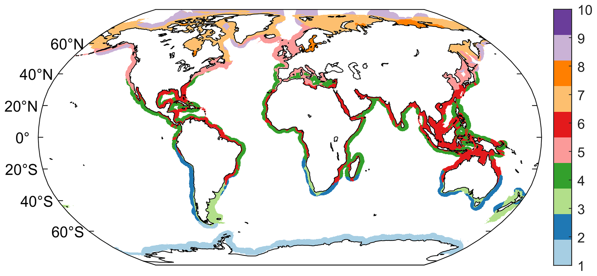
Figure 1Coastal biogeochemical provinces generated by the Self-Organizing Maps (SOM) clustering algorithm. The spatial extension of these provinces can vary from one month to another due to seasonal variations of the environmental drivers used during SOM. Here we present their modal spatial distribution (see Sect. 2.1 for further details).
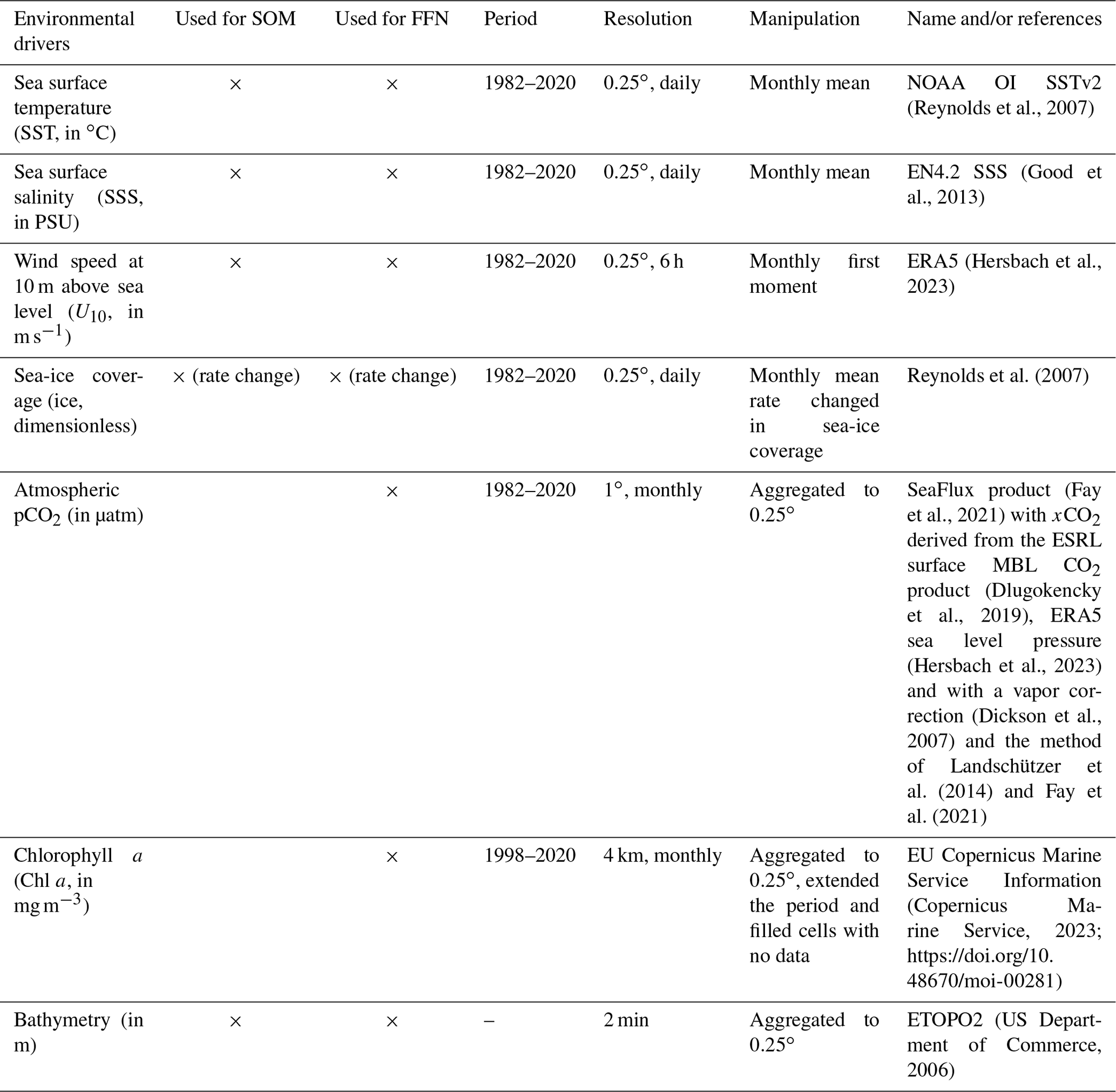
Table 1Environmental drivers used for the Self-Organizing Maps (SOM) and the Feed-Forward Network (FFN) artificial neural networks to reconstruct the coastal pCO2. These datasets are also used to calculate the coastal air–sea CO2 exchange.
In a second step, within each biogeochemical province identified in step 1 (SOM), a FFN algorithm establishes nonlinear relationships between the observed sea surface pCO2 and independent variables, or drivers, that are known to control its spatial and temporal variability. For each province, the FFN algorithm calculates relationships between the observed target variable (here pCO2 using pCO2 observations from the SOCAT_a dataset; see below) and inputs (environmental drivers; see below and Table 1) by adjusting weighting factors of a sigmoid activation function (one sigmoid function per neuron in the hidden layer) following an iterative procedure, i.e., a Levenberg–Marquardt backpropagation algorithm. At the first iteration, the weights of neurons are randomly assigned and the reconstructed pCO2 is compared with the actual pCO2 observations. Based on the resulting mismatch, the network weights are iteratively updated in a way that the error function – in our case the mean squared error between network output and actual observations – gets minimized. For each iteration, the FFN algorithm uses a fraction of the pCO2 observations for the actual training of the network (i.e., the adjustment of the neuron weights), while another randomly selected fraction of the dataset is used to independently evaluate the performance of the algorithm. The final coefficients are obtained when the reconstructed pCO2 simulated from the validation data does not significantly improve relative to the pCO2 observations, to prevent overfitting. The final neuron weights and thus the resulting input–output relationships are used to reconstruct pCO2 in each cell and for each month during the 1982–2020 period.
The predictors used for the FFN are U10, SST, SSS, the atmospheric pCO2, the rate of change in sea-ice coverage (except in regions not covered by sea ice, i.e., in P2, P3, P4 and P6), the bathymetry and the chlorophyll a concentration (Chl a). The Chl a is expressed as log10(Chl a) to minimize the influence of its skewed distribution (Wrobel-Niedzwiecka et al., 2022). In P1, P8 and P9, we do not use Chl a as a driver because of the poor data coverage resulting from recurring cloud and/or sea-ice coverage in those provinces (see Sect. 2.2). This incomplete data coverage for Chl a is incidentally the reason why this predictor is not used at the SOM stage, because it requires complete global datasets. Atmospheric pCO2, which was not included in the ULB–SOM–FFN–coastalv1, is also used as a driver of multidecadal changes induced by the increasing atmospheric pCO2 concentration. Finally, we smooth spatially the monthly-resolved coastal pCO2 field generated by the FFN using a moving 3 by 3 pixel window to remove abrupt pCO2 transitions sometimes occurring at the boundaries between provinces. This smoothing procedure is described by Landschützer et al. (2014) and was also used in the ULB–SOM–FFN–coastalv1.
The surface pCO2 data are extracted from the SOCATv2022 database (Bakker et al., 2022) that originally contains ∼40 million pCO2 measurements for the entire global ocean (open and coastal seas combined). We randomly divide this dataset into two independent datasets: a group of data used for the FFN algorithm (SOCAT_a; see below) and a group of data that we use to validate our reconstructed pCO2 (SOCAT_b). To do so, from the SOCATv2022 database, we follow the recommendation of the SOCAT community and use their accuracy criteria to only retain the data with the highest accuracy. To do so, we first select sea surface measurements expressed in fugacity of CO2 (fCO2) with a quality flag ranging from A to D (which corresponds to an estimated accuracy better than 5 µatm) and a World Ocean Circulation Experiment (WOCE) flag of 2 (good dataset following SOCAT) for the 1982–2020 period. Following Laruelle et al. (2017), we also remove fCO2 values <30 and >1000 µatm that are likely derived from estuarine or fresh water systems that are not included in our coastal domain. We then randomly divide this dataset rich of ∼32 million fCO2 measurements into a group of data used for the FFN algorithm (“a”, 80 % of the original dataset) and a group of data that we use to validate our reconstructed pCO2 (“b”, 20 % of the original dataset). The two sets of data (SOCAT_a and SOCAT_b) are then gridded for each month at 0.25∘ using the average of all fCO2 values in each cell. Values are then converted from fCO2 to pCO2 using the equation of Takahashi et al. (2019, p. 7) and a coastal mask is applied on both gridded pCO2-products. In this study, the coastal domain (“wide coastal ocean” with a total surface area of 76×106 km2, Laruelle et al., 2017) excludes the Black Sea, estuaries as well as inland water bodies, and its outer limit is defined as whichever point is furthest from the shoreline between the 1000 m isobath and a fixed 300 km distance (roughly the outer edge of territorial waters), following the coarse SOCAT definition of the coastal oceanic domain. At the end of this entire procedure, a total of ∼14 million and ∼4 million discrete coastal data have been allocated to SOCAT_a and SOCAT_b, respectively. A more common delineation of the coastal ocean is also used in this study when discussing the air–sea CO2 exchange (Sect. 3.1) using the shelf break as the outer limit of the coastal domain (“narrow coastal ocean”, 28×106 km2). The depth of the shelf break is calculated using a high-resolution global bathymetric database and estimated by calculating the slope of the sea floor. The isobath for which the increase in slope is the maximum over the 0–1000 m interval, yet still inferior to 2 %, defines the outer limit of the shelf break (Laruelle et al., 2013).
2.2 Environmental variables
The observational SST and SSS fields used as inputs for the SOM–FFN algorithm are calculated as the monthly means of the daily NOAA OI SST V2 (Reynolds et al., 2007) and of the daily Hadley center EN4 SSS (Good et al., 2013), respectively (Table 1). For U10, we use the monthly mean of the 0.25∘ resolution product of the European Center for Medium-Range Weather Forecasts (ECMWF) ERA5 wind product (Hersbach et al., 2023), which has a native temporal resolution of 6 h. The monthly mean of the daily 0.25∘ dataset of Reynolds et al. (2007) is used for the sea-ice coverage. The rate of change in the sea-ice coverage for a given month x is then calculated as the difference between the sea-ice coverages of months x+1 and x−1. The atmospheric pCO2 is from the SeaFlux product (Fay et al., 2021) which is calculated from the dry air mixing ratio of CO2 (xCO2) provided by the ESRL surface marine boundary layer CO2 product (Dlugokencky et al., 2019; https://www.esrl.noaa.gov/gmd/ccgg/mbl/data.php; last access: October 2023) with a vapor correction according to Dickson et al. (2007), using the ERA5 sea level pressure (Hersbach et al., 2023) and applying the method of Landschützer et al. (2014) and Fay et al. (2021). It should be noted that, due to the proximity to the continent, the coastal ocean might be more exposed to anthropogenic sources of CO2 and thus might be exposed to higher atmospheric pCO2 compared with the global oceanic average. The use of spatially resolved dry air mixing ratio of CO2 datasets, such as the one from the NASA's Orbiting Carbon Observatory 2 Goddard Earth Observing System (OCO-2 GEOS; Eldering et al., 2017), instead of the product used in this study might be more appropriate to include this effect. However, OCO-2 GEOS only covers 2015–2022, which is too short for the purpose of our study. It is also expected that the choice of the atmospheric pCO2 does not considerably influence our FCO2 calculations as the air–sea pCO2 difference is mainly controlled by the oceanic pCO2 (see Sect. 2.4). We use the bathymetry from the 2 min global ETOPO2 database (US Department of Commerce, 2006) and the Chl a field derived from the monthly 4 km merged GlobColour product from the EU Copernicus Marine Service information (Copernicus Marine Service, 2023; https://doi.org/10.48670/moi-00281, last access: October 2023), which is the product with the longest Chl a temporal coverage (1998–2020). However, because of recurrent cloud coverage everywhere and sea-ice coverage at high latitudes, the monthly averaged Chl a field at a 0.25∘ resolution is discontinuous with grid cells devoid of data. We fill these cells (9 % excluding high latitude coastal regions) using a cascade of interpolation methods, the order of which depends on data availability in time and space in the surrounding cells: for an empty cell of the month x, the interpolation is performed by computing in the order of rank (1) the mean of the next neighboring cells of the month x, (2) the mean value of the month x+1 and month x−1 of the same cell, (3) the monthly mean value x of the cell for the entire 1998–2020 period and (4) the annual mean value of the cell for the entire 1998–2020 period. At high latitudes, where none of these options are feasible because of large bands without any data, we assign the modal value of Chl a as the default value in order to ensure the continuity of the maps that is required for the FFN algorithm. From this continuous gridded Chl a product over the recorded period, we then calculate for each cell a monthly seasonal climatology and attribute the climatological values to the unrecorded period (1982–1997). This means that, in our calculations, Chl a does not contribute to long-term changes in pCO2 before 1997. All observational fields are converted from their original spatiotemporal resolution to monthly 0.25∘ gridded resolution for the 1982–2020 period (except for the bathymetry which is constant over time) to match the observational pCO2-product (SOCAT_a) resolution (Table 1).
2.3 Air–sea CO2 exchange
The pCO2 field generated by the SOM–FFN algorithm (ULB–SOM–FFN–coastalv2) is used to calculate the air–sea CO2 exchange for each grid cell at the monthly timescale over the 1982–2020 period following Eq. (1):
where FCO2 (mol C m−2 yr−1) represents the coastal air–sea CO2 exchange, ΔpCO2 (atm) is the gradient between the oceanic pCO2 and the atmospheric pCO2 and K0 (mol m−3 atm−1) is the CO2 solubility in seawater which is a function of SST and SSS following the equation of Weiss (1974). k (m yr−1) represents the gas exchange transfer velocity which is a function of the second moment of the wind speed at 10 m above sea level and is calculated using the equation of Ho et al. (2011) and using the Schmidt number based on the equation of Wanninkhof (2014). The sea-ice coverage for each grid cell is represented by the term ice and ranges from 0 (no ice cover) to 1 (100 % ice cover). By convention a positive FCO2 value corresponds to a source of CO2 for the atmosphere. We use the same U10, SST, SSS, sea-ice coverage and atmospheric pCO2 datasets (see Sect. 2.2) to calculate FCO2 and perform the FFN pCO2-reconstruction. Our reconstructed coastal FCO2 is also compared with coastal FCO2 estimates derived from a synthesis of 214 regional FCO2 estimations (Dai et al., 2022) and from the FCO2-product derived from the original ULB–SOM–FFN–coastalv1 pCO2-product (Roobaert et al., 2019).
2.4 Uncertainties in the reconstructed coastal data products
The uncertainties associated with our reconstructed pCO2 and FCO2 coastal products are estimated using the method proposed by Landschützer et al. (2014, 2018) and used by subsequent authors (e.g., Roobaert et al., 2019; Sharp et al., 2022). The FCO2 uncertainty results from four sources of uncertainties, which are considered independent and thus summed quadratically:
where represents the total FCO2 uncertainty (Pg C yr−1), is the uncertainty of the air–sea pCO2 gradient, σk is the uncertainty associated with the choice of the k formulation in Eq. (1) and σwind is the uncertainty associated with the choice of the wind speed product (see Roobaert et al., 2018). We also include the effect of the choice of sea-ice product on the FCO2 uncertainty (σice) which was not included in the original calculations of Landschützer et al. (2014, 2018) but has been identified as a potential source of uncertainty in global coastal reconstructions (e.g., Resplandy et al., 2023). All of these four sources of uncertainty are expressed in petagrams of carbon per year. We do not include the uncertainty associated with the solubility term (K0) in our uncertainty assessment since this contribution is minimal (0.2 %) as suggested by Weiss (1974). σwind is calculated following the strategy described in Roobaert et al. (2018) which consists of using the standard deviation of global FCO2 fields calculated with three different wind products: the ERA5 (Hersbach et al., 2023), the Cross-Calibrated Multi-Platform Ocean Wind Vector 3.0 (Atlas et al., 2011) and the NCEP/NCAR reanalysis 1 (Kalnay et al., 1996). Since these wind products cover different time periods, σwind is calculated for the overlap period (1991–2011) between products. σk is estimated as the standard deviation of global FCO2 fields calculated with four different global scale k parametrizations with the same wind speed (ERA5). We use the formulations of Ho et al. (2011), Sweeney et al. (2007), Takahashi et al. (2009) and Wanninkhof (2014), all suited for global scale applications (e.g., see Roobaert et al., 2018). σice is calculated as the standard deviation of global FCO2 fields calculated with two different sea-ice products: the NOAA dataset of Reynolds et al. (2007) and the sea-ice dataset of Rayner et al. (2003). mainly results from the oceanic pCO2 uncertainty since the atmospheric pCO2 uncertainty is significantly lower (Landschützer et al., 2018). For instance, Roobaert et al. (2019) quantified that uncertainties in atmospheric pCO2 only contribute to 6 % in the overall FCO2 uncertainty.
Following Landschützer et al. (2014), the uncertainty over the oceanic pCO2 can be obtained from the quadratic sum of three sources of uncertainties:
where represents the total uncertainty of the oceanic pCO2 (µatm), θobs is the experimental uncertainty associated with the sampling in the field of the observations from the SOCAT database (µatm), θgrid is the uncertainty associated with the gridding of the observations from SOCAT into 0.25∘ monthly meshed maps (µatm) and θmap is the uncertainty derived from the comparison between the reconstructed pCO2 and the observed gridded pCO2 from the SOCAT database (µatm). Following Sharp et al. (2022), we use accuracies that are attributed to each fCO2 measurement by the SOCAT community (flags A–D) to calculate θobs. Flags “A” and “B” represent an estimated accuracy of 2 µatm while the accuracy of flags “C” and “D” is 5 µatm. We first calculate the mean of all fCO2 flags in each grid cell for each month. We then calculate the global average gridded flags uncertainty of all cells for the year x (or the entire period). For θgrid, we first calculate in each grid cell of the month x the standard deviations of all fCO2 values from the SOCAT database used for the gridding. We then calculate the average of these standard deviations of all grid cells for the year x (or the entire period). θmap is calculated as the root mean squared deviation between the reconstructed pCO2 and the gridded pCO2 observation from the training dataset (SOCAT_a). We also divide each source of uncertainty (i.e., θobs, θgrid and θmap) by the square root of the number of pCO2 samples (N; for details see Landschützer et al., 2018; Roobaert et al., 2019). For θmap, the value of N is corrected to account for the fact that all individual errors are not spatially independent. To this end, we calculate the effective sample size (Neff; see Landschutzer et al., 2018) by randomly selecting 1000 samples (40 % of the samples if the total number of samples is <1000) that cover our study period and calculating a lag 1 autocorrelation coefficient following Eqs. (18) and (19) of Landschützer et al. (2018). As we only use a subset of 1000 samples, we perform Monte Carlo simulations where this procedure is repeated 10 times and our final Neff is calculated as the median of the 10 iterations. Finally, the total uncertainty on FCO2 associated with the reconstructed pCO2 (, Pg C yr−1) is obtained by applying (µatm) in Eq. (1). All these procedures are performed globally for each year and for the entire period of our study.
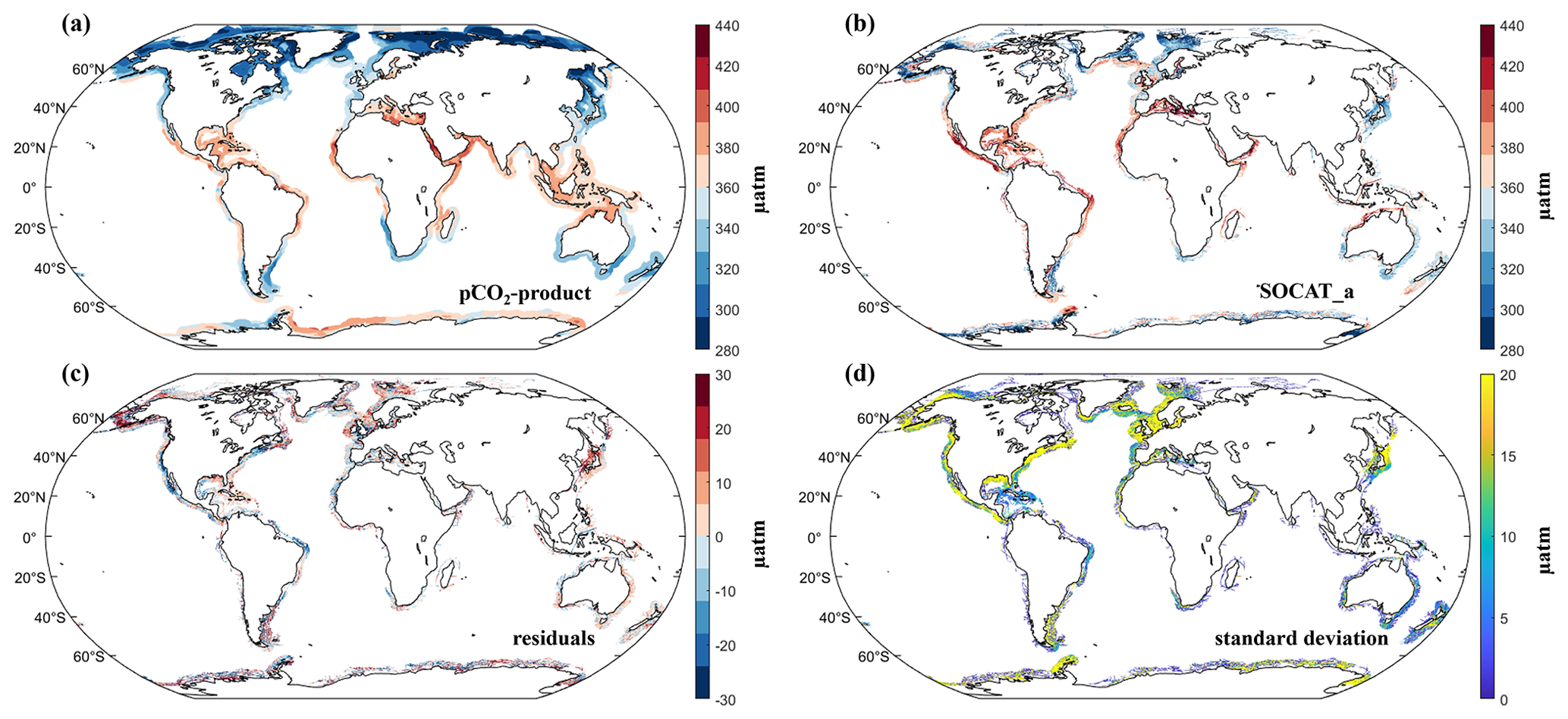
Figure 2Global maps of the climatological (1982–2020) averaged (a) reconstructed coastal pCO2-product and (b) gridded pCO2 from the SOCATv2022 database and used for the FFN algorithm (SOCAT_a). Panel (c) shows the temporal mean of the residuals between the coastal pCO2-product and SOCAT_a and (d) shows standard deviation. Values in all panels are expressed in µatm.
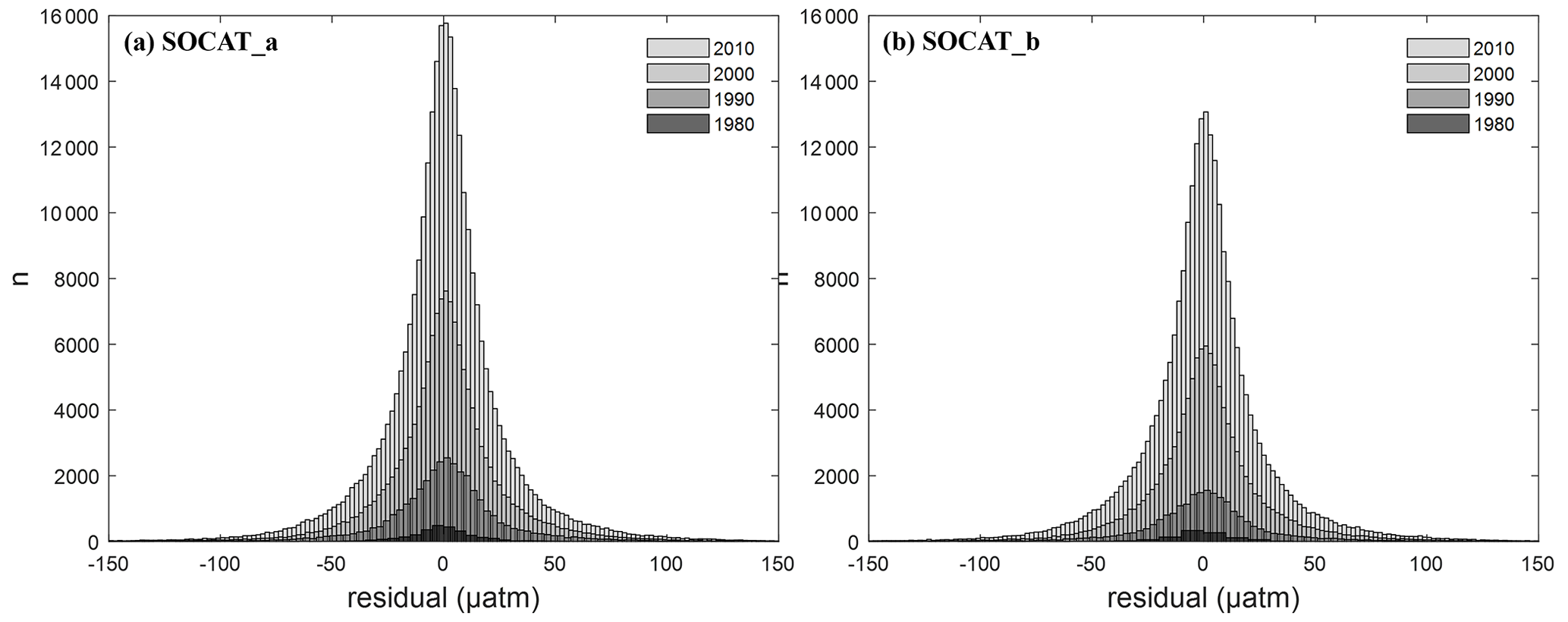
Figure 3Histograms of the pCO2 residuals (difference between the reconstructed coastal pCO2-product with (a) SOCAT_a and (b) SOCAT_b) for four decades expressed in µatm.
3.1 pCO2-product evaluation
Globally, our reconstructed coastal pCO2-product compares well with the observed pCO2 used to train the FFN algorithm (SOCAT_a) and reproduces all the well-known global spatial pCO2 patterns with generally low pCO2 (<360 µatm) at temperate as well as high latitudes and high pCO2 (> 360 µatm) at low latitudes (contrast Fig. 2a with Fig. 2b). The spatial distribution of the temporal mean residuals (i.e., difference between the coastal pCO2-product and SOCAT_a in each grid cell for every month where observations are available) reveals that, in some regions, underestimations (negative mean residual; blue colors in Fig. 2c) or overestimations (red colors) of the pCO2 can be generated by the coastal pCO2-product. However, most of the calculated residuals fall within the −20 to 20 µatm range, accounting for 69 % of the grid cells, while 45 % of the grid cells have absolute residuals <10 µatm (Figs. 2c and 3a).
A global mean of the residuals (bias) value of 0 µatm and a coefficient of determination (r2) of 0.7 are calculated, as expected, since the algorithm minimizes the root mean square error (RMSE) between the reconstructed pCO2 and target pCO2 observations. The global RMSE is, however, substantially larger (29 µatm) yet still comparable to those calculated, at the regional scale, in previous coastal pCO2 studies based on statistical interpolations (e.g., see Chen et al., 2016) and slightly lower than the 32 µatm global RMSE calculated by Laruelle et al. (2017). Large differences can be observed between our product and SOCAT_a locally in regions that are known to present large spatiotemporal variabilities in pCO2 and/or in regions lacking data to train our FFN algorithm. For instance, residuals and/or standard deviations >20 µatm are encountered in the Baltic Sea (which is henceforth treated as an independent biogeochemical province for some calculations), in upwelling regions (e.g., along the Peruvian upwelling), in coastal seas under the influence of seasonal changes in sea-ice coverage (e.g., along the Antarctic shelf) as well as along the very nearshore coastal domain (e.g., along the California current coast; Fig. 2c and d).
The overall consistency between our coastal pCO2-product and SOCAT_a is diagnosed over the entire time span of our study, as illustrated by the histograms of residuals calculated for each of the four decades of our calculation period (Fig. 3a) or when the calculations are performed for each individual year (Table S1 in the Supplement). This is an important test as a study by Gloege et al. (2022) suggests that decadal trends in pCO2-products may be obscured by changing residual distributions over time. In spite of the highly heterogeneous distribution of the number of pCO2 observations available through time (<500 gridded cells in the 1980s vs. >10 000 in the 2010s), the shape and spread of the four histograms of the residuals are closely similar between decades with a distribution centered on a global mean bias close to 0 µatm and most of the residuals falling in the −20 and 20 µatm range. This demonstrates the accuracy of the method over time despite the skewed distribution of the calibration data. The analyses performed for each individual year reveal that global biases do not exceed 5 µatm. Exceptions are observed in the 1980s where biases (e.g., absolute bias of 6 µatm in 1987) and RMSE (e.g., 42 µatm in 1989) can be larger and partly attributed to an exceptionally low pCO2 observational coverage during these periods (e.g., see Bakker et al., 2014). In the first version of the coastal product (ULB–SOM–FFN–coastalv1), the evaluation of the pCO2-product of Laruelle et al. (2017) was restricted to spatial and climatological seasonal cycles. In this study, we successfully extended this analysis to the entire time period and evaluated each year and decade individually.
Table 2Statistical analyses (bias, RMSE and r2) of the reconstructed coastal pCO2-product compared with pCO2 observations from SOCAT_a and SOCAT_b for the different biogeochemical provinces. For each province, bias, RMSE and r2 are calculated using all of the monthly cells of the province for the period 1982–2020.
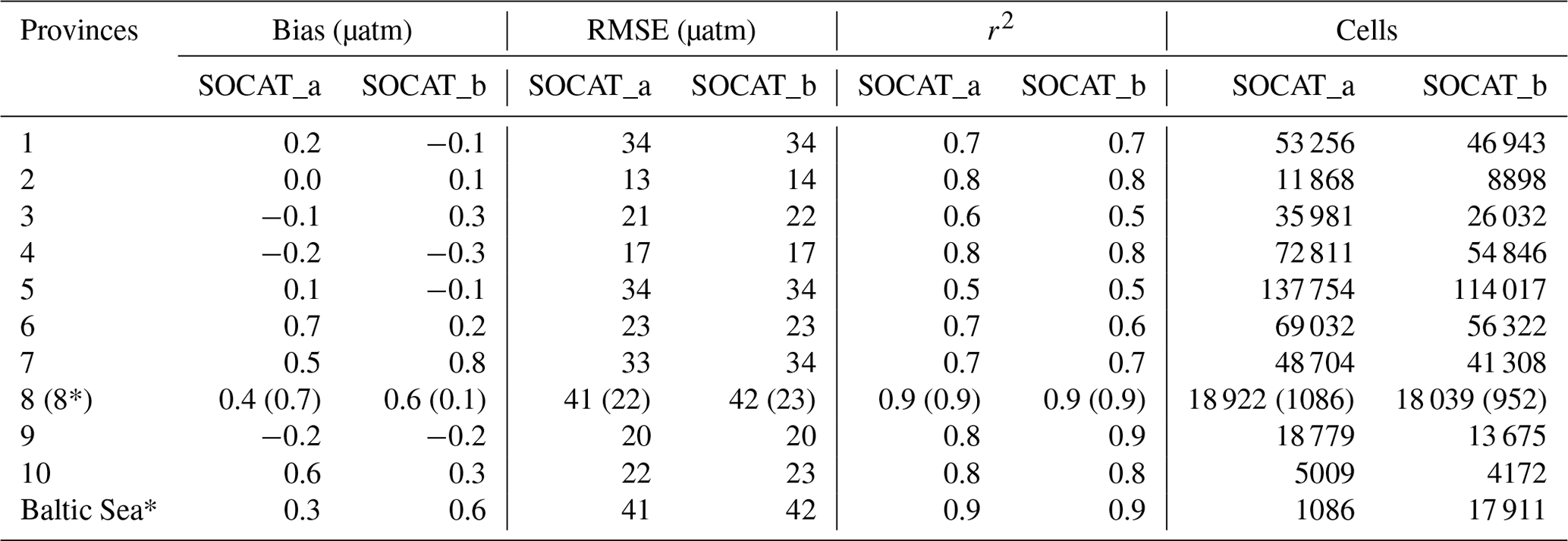
* Numbers in parentheses for P8 represent statistics when the Baltic Sea is removed from P8 and defined as an isolated province.
At the regional scale, 7 out of the 10 biogeochemical provinces yield RMSEs against SOCAT_a close to 20 µatm or lower with the best fit in P2 (RMSE = 13 µatm; Table 2). This is a significant improvement over the ULB–SOM–FFN–coastalv1 product which only had three provinces with RMSE <20 µatm (Laruelle et al., 2017) and none <15 µatm. We attribute this improvement to our advanced setup of the method such as the inclusion of the atmospheric pCO2 as a driver as well as an increased number of available observations to train our FFN algorithms. In three provinces (P1, P5 and P7), however, the RMSE exceeds 35 µatm. Such values can partly be explained by the complex dynamics of the sea ice in the Antarctic shelf (P1) and by the limited number of observational data combined with the inclusion of coastal regions that present large spatiotemporal variabilities and cover two disconnected temperate basins (P5 and P7) of the Northern Hemisphere. This discrepancy was also highlighted by Landschützer et al. (2020). High discrepancies are further observed in the Baltic Sea (Fig. 2c and d) which is analyzed as a separate province (RMSE value of 41 µatm; Table 2). Excluding the Baltic Sea from P8 considerably reduces RMSE from 41 to 23 µatm. The inclusion of the Baltic Sea in P8 can also explain the large RMSE calculated by Laruelle et al. (2017) for the corresponding province of the ULB–SOM–FFN–coastalv1 coastal pCO2-product (∼47 µatm).
3.2 Validation against independent data
Our reconstructed coastal pCO2-product is also validated against an independent dataset that is derived from pCO2 observations from the SOCATv2022 that were not used for the training of the FFN algorithm (see Sect. 2.1). This dataset consists of a pool of 404 206 gridded cells that are uniformly distributed between both hemispheres (SOCAT_b; Fig. S1 in the Supplement), an essential criterion for training the network. Globally, a good match is observed between the coastal pCO2-product and SOCAT_b with a global bias and an RMSE of 0 and 29 µatm, respectively. These values are similar to those derived from the statistical analysis performed against SOCAT_a. At the biogeochemical provinces scale, RMSEs generally do not exceed 23 µatm (maximum value in P6; Table 2), except where important RMSEs (34 µatm for P1, P5 and P7) had already been calculated during the comparison with SOCAT_a (i.e., in regions under the sea-ice coverage dynamics and poor data coverage and provinces which encompass regions with high spatiotemporal pCO2 dynamics).
As with SOCAT_a, the analysis against SOCAT_b demonstrates a good performance of our reconstructed coastal pCO2-product over time with the histograms of the residuals calculated for each of the four decades presenting the same shape and spread in spite of the marked decrease in grid cell numbers over time (1054 grid cells in 1980 vs. 248 626 grid cells in 2010; Fig. 3b). Each of these histograms shows a distribution centered on a value of 0 µatm with ∼50 % of the grid cell residuals falling between −10 and 10 µatm. This is also true at the scale of the biogeochemical provinces with the four histograms of the residuals revealing global mean biases of 0 µatm and ∼50 % of the residual falling in the −10 and 10 µatm range. Only P8 stands as an exception (where 50 % of the residuals are between −40 and 40 µatm; Fig. S2), mainly due to the presence of the Baltic Sea in this province.
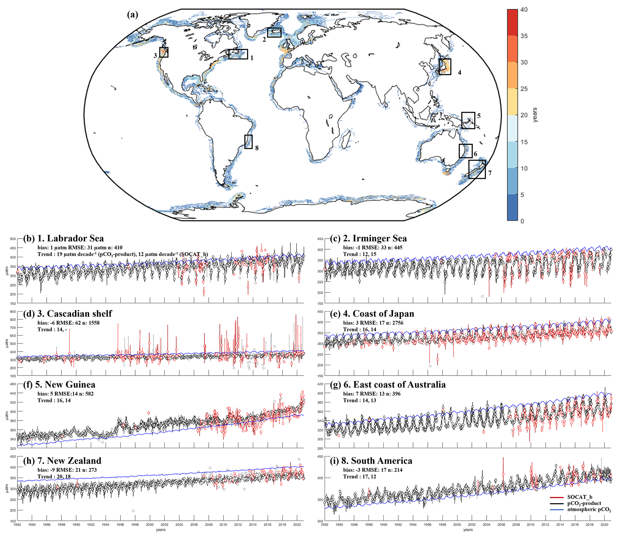
Figure 4Panel (a) shows the temporal coverage (in years) where pCO2 measurements extend over x years in SOCAT_b. The location of the eight coastal sites for which we present pCO2 times series (black boxes) is also shown. Panels (b–i) show pCO2 times series (in µatm) from the reconstructed pCO2-product (in black), from SOCAT_b (in red), and from the atmospheric pCO2 (in blue). For each region, we only select grid cells that extend over 30 years of observations in SOCAT_b. Medians are represented by circles and the vertical bars represent the monthly pCO2 intra-spatial variability in the region. For each region, we report the bias (µatm), RMSE (µatm) and number of cells for the calculation between the reconstructed pCO2-product and SOCAT_b as well as their respective long-term pCO2 trend (in µatm decade−1, which is calculated first as the slope of a linear trend using the monthly median values of all the deseasonalized data). The Cascadian shelf has no value for the SOCAT_b trend since no significant trend is detected based on a Mann–Kendall statistical test.
We also present pCO2 time series derived from our reconstructed coastal pCO2-product and compare them to data extracted from SOCAT_b for eight coastal sites (Fig. 4). The choice of these coastal regions is motivated by their data coverage extending over 30 years (Fig. 4a) and the fact that it is possible in these grid cells to reconstruct a spatially complete seasonal climatological cycle (i.e., data are available for all 12 months). For each region, we only extracted cells for which observations extended >30 years and reconstructed their times series from the coastal pCO2-product and SOCAT_b, respectively (Fig. 4b–i). For most of the regions, the pCO2-product properly captures the temporal dynamics of pCO2 derived from the observations, bearing slight underestimations or overestimations in specific areas such as along the Cascadian shelf and the east coast of Australia (Fig. 4d and g). For the eight coastal sites, absolute biases are all <10 µatm with a minimum absolute bias of 1 µatm in the Irminger Sea and a maximum absolute bias of 9 µatm along the New Zealand coast. Except along the Cascadian shelf, all coastal sites present RMSEs lower than ∼30 µatm (five of the eight regions show RMSEs µatm) which falls in the range of our global and regional RMSE values. The largest RMSE is calculated along the Cascadian shelf (62 µatm) and can partly be explained by the large spatial pCO2 variability in SOCAT_b (as shown by the vertical bars in Fig. 4d) because of the riverine influence in the region.
Finally, the reconstructed pCO2 times series are compared with three buoys with measurements longer than 10 years located in Cape Elizabeth (NDBC Buoy 46041), in Gray's Reef (NDBC Buoy 41008) and in the Gulf of Maine (Coastal Western Gulf of Maine Mooring; Sutton et al., 2019). The three pCO2 time series for each buoy location mentioned above are presented in Fig. S3. Although smaller amplitude variabilities are generally observed, results show that the reconstructed pCO2 times series follow those of the observational data with values that are mainly between the buoys errors (Fig. S3a–c). We speculate that the smaller amplitude stems from the coarser 0.25∘ grid resolution of our method compared with the point nature of the buoy data. Landschützer et al. (2016) drew a similar conclusion when they compared their open ocean pCO2 data with open ocean at HOT and BATS and is further corroborated by the much smaller variabilities obtained when raw SOCAT data are averaged at the grid cell level (Fig. 4). The exception is the Gulf of Maine where a general underestimation of pCO2 is observed compared with the buoy observations. The reconstructed pCO2-product also reproduces the observed climatological seasonal cycles (including a relatively good timing of the seasonal maxima and minima) for the three buoys as shown in Fig. S3d–f. Absolute average bias values of 14, 4 and 45 µatm, and RMSE values of 50, 53 and 61 µatm, are calculated between the pCO2-product and the observations for Cape Elizabeth, Gray's Reef and in the Gulf of Maine, respectively. These statistical error values are larger than those calculated when the comparison with SOCAT is performed, whether on a global or regional scale. This is not surprising since the reconstructed pCO2-product is for a global application and is quite challenging to compare with specific coastal buoys that present high temporal and spatial variability such as shown by the violin in Fig. S3.
The good evaluation of the reconstructed pCO2 compared with SOCAT_a, SOCAT_b and buoys data gives us confidence to identify the linear trends of both the pCO2 and FCO2 over different temporal scales. For example, our results show that for all the eight studied regions represented in Fig. 4, an increase in pCO2 over time comprised between 12 and 20 µatm decade−1 is calculated for the long-term trend with our pCO2-product, a range in good agreement with the 12–18 µatm decade−1 obtained with SOCAT_b. Although New Zealand shows the largest bias between SOCAT_b and the pCO2-product, they both show that this region displays the fastest trend in terms of pCO2 rise (18 and 20 µatm decade−1 for SOCAT_ b and the pCO2-product, respectively).
3.3 Air–sea CO2 exchange
This section describes the coastal air–sea CO2 exchange patterns that are calculated using our new reconstructed pCO2-product over the 1982–2020 period. The spatial and seasonal FCO2 patterns are only briefly discussed (Sect. 3.3.1) since those have been extensively discussed in previous studies (e.g., see Dai et al., 2022; Resplandy et al., 2023; Roobaert et al., 2019). We thus focus on the long-term FCO2 trends (Sect. 3.3.2), which are still poorly understood and highly debated (e.g., Lacroix et al., 2021a; Laruelle et al., 2018; Resplandy et al., 2023).
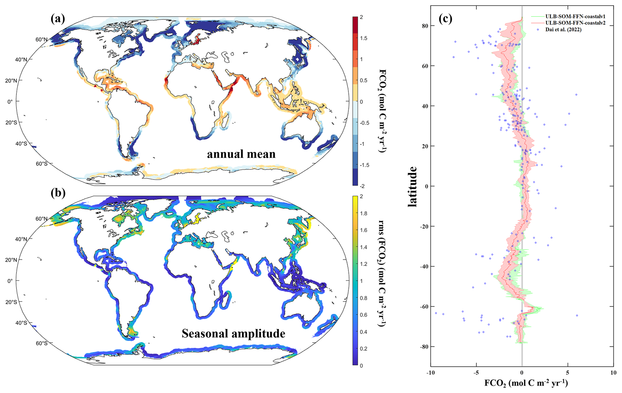
Figure 5Panel (a) shows the spatial distribution of the annual average air–sea CO2 exchange (FCO2, in mol C m−2 yr−1) and (b) seasonal FCO2 variability (expressed as the root mean square (RMS, in mol C m−2 yr−1)) calculated with the reconstructed coastal pCO2-product (ULB–SOM–FFN–coastalv2, 1982–2020 climatology). The latitudinal mean FCO2 distribution (red line) and its associated longitudinal variability (red shading) is presented in panel (c). This latter is compared with the FCO2 calculated with the ULB–SOM–FFN–coastalv1 pCO2-product (in green; Roobaert et al., 2019) and against a synthesis of 214 regional FCO2 estimations (blue dots; Dai et al., 2022). For consistency in the comparison in (c) we applied the same coastal delimitation as in Dai et al. (2022) and Roobaert et al. (2019) to the FCO2 ULB–SOM–FFN–coastalv2 product, i.e., we used the shelf break as the outer limit of the coastal domain (narrow coastal ocean). Panel (c) is also reconstructed based on an overlap period between the three products (1998–2020; except FCO2 ULB–SOM–FFN–coastalv1 which is limited to the 1998–2015 period).
3.3.1 Spatial and seasonal variations
The spatial distribution of the climatological mean coastal FCO2 shows that coastal regions in temperate areas (between 40 and 60∘ in both hemispheres) and at high latitude (beyond 60∘ in both hemisphere) mainly act as CO2 sinks while CO2 sources are mainly encountered in the subtropical band (Fig. 5a) which is consistent with the global latitudinal pattern established by previous studies (e.g., Borges, 2005; Borges et al., 2005; Cai, 2011; Cao et al., 2020; Chen et al., 2013; Dai et al., 2022; Laruelle et al., 2010, 2014; Roobaert et al., 2019). Globally, with the coastal delineation used in this study (“wide coastal ocean”; 76×106 km2), the coastal ocean absorbs on average 0.40 Pg C per year (with an uncertainty of ±0.03 Pg C yr−1; see Sect. 3.3.3) over the 1982–2020 period. Using the shelf break as the outer limit of the coastal domain (“narrow coastal ocean”; 28×106 km2) which is a more common delineation of the coastal ocean, the globally integrated coastal sink amounts to Pg C yr−1 which is consistent with the latest estimates (e.g., −0.2 Pg C yr−1 in Roobaert et al., 2019, and −0.25 Pg C yr−1 in Dai et al., 2022). It should be noted that these comparisons are not straightforward because they do not cover the same time periods (i.e., the 1998–2015 period in Roobaert et al. (2019), 1998 to the present in Dai et al. (2022) and 1982–2020 in this study) and older assessments often do not report an explicit calculation period (Regnier et al., 2022).
Most of the intense CO2 sinks (absolute FCO2 value >0.5 mol C m−2 yr−1) are encountered at high latitudes of the Northern Hemisphere and in the temperate regions of the Southern Hemisphere, while CO2 sources in the tropical bands are moderate except along upwelling areas such as in the Arabian Sea (Fig. 5a and c). A large fraction (44 % and 53 % for the wide and narrow domain, respectively) of the global CO2 uptake is taking place north of 60∘ N, which was already suggested in Laruelle et al. (2010) and further confirmed in subsequent studies (e.g., Cai, 2011; Dai et al., 2022; Laruelle et al., 2014; Roobaert et al., 2019). The spatial distribution of coastal CO2 sources and sinks also closely follows the latitudinal FCO2 profile calculated by Roobaert et al. (2019) which is based on ULB–SOM–FFN–coastalv1 (red and green lines in Fig. 5c). These global pCO2-products, however, predict less variability in flux density than a compilation of regional estimations as shown in Fig. 5c when comparing our climatological FCO2 latitudinal profile with the synthesis of 214 regional FCO2 estimates which was already pointed by Dai et al. (2022) when comparing their data synthesis with the latitudinal FCO2 profile of Roobaert et al. (2019), suggesting strong FCO2 heterogeneities for a same latitudinal band. Finally, the seasonal coastal FCO2 variability (expressed as the root mean square (RMS) of the seasonal amplitude) agrees with the few studies performed at global scale (e.g., see Dai et al., 2022; Roobaert et al., 2019) with high seasonal FCO2 amplitudes (RMS values >1.5 mol C m−2 yr−1) at temperate and high latitudes and a low amplitude over the subtropical band (Fig. 5b).
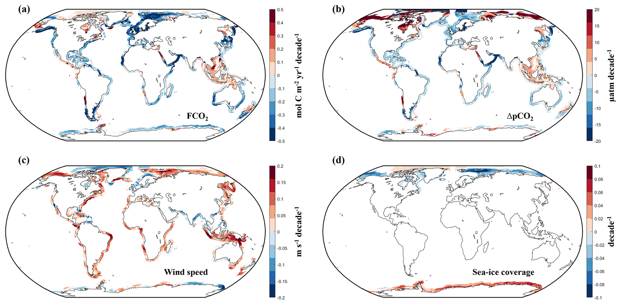
Figure 6Long-term trend in (a) the coastal FCO2 (in mol C m−2 yr−1 decade−1), (b) the air–sea pCO2 gradient (ΔpCO2, in µatm decade−1), (c) the wind speed at 10 m above the sea surface (m s−1 decade−1) and (d) the sea-ice coverage (decade−1) from 1982 to 2020. For each panel, the long-term trend is calculated as the slope of a linear regression on the monthly median values of all the deseasonalized data from 1982 to 2020. We only present grid cells where a significant trend is detected based on a Mann–Kendall statistical test.
3.3.2 Long-term trends in the coastal CO2 sink
The rate of change in coastal FCO2 and the various parameters involved in the FCO2 calculation (i.e., ΔpCO2, wind speed and sea-ice coverage) from 1982 to 2020 are presented in Fig. 6. Our results reveal significant spatial heterogeneities between the long-term temporal FCO2 trends (linear trends that span over 39 years) observed within different coastal regions, a finding consistent with the range of varying slopes (including changes in sign of the slopes) already reported in local regional and discontinuous global studies (e.g., Becker et al., 2021; Laruelle et al., 2018; Wang et al., 2017). Our results also show that the rates of changes in ΔpCO2 and FCO2 follow each other (compare Fig. 6a with 6b). Coastal regions with negative (positive) ΔpCO2 slopes present negative (positive) FCO2 slopes, which translate into a stronger sink/weaker source (weaker sink/stronger source). Most coastal regions (∼60 % of the grid cells that present a significant trend using a Mann–Kendall statistical test with a significance threshold of 95 %) exhibit negative ΔpCO2 and FCO2 slopes (i.e., stronger sinks or weaker sources; blue colors in Fig. 6a and b) in agreement with past studies (e.g., Laruelle et al., 2018; Resplandy et al., 2023; Wang et al., 2017). Positive ΔpCO2 and FCO2 slopes (weaker sink or stronger sources; red colors) can also be observed such as along the Mediterranean Sea or Southeast Asia. Stronger FCO2 rates of change (absolute value >0.6 mol m−2 yr−1 decade−1) are mainly observed in mid to high latitude coastal regions and along upwelling regions (e.g., Moroccan upwelling current), while low latitude coastal regions show weaker slopes.
Although our results suggest that the long-term change in FCO2 intensity mainly results from that of the ΔpCO2 (compare Fig. 6a with 6b), the rate of change in FCO2 can be amplified or dampened in some regions by changes in wind speed patterns and/or sea-ice coverage (through their effect on Eq. 1), in agreement with recent findings by Resplandy et al. (2023). For most of the coastal ocean, an increase in wind speed has been observed over the study period (positive slope, red colors in Fig. 6c) with a median value for the rate of change value of 0.04 m s−1 decade−1. This increase in wind speed promotes the FCO2 exchange through its effect on the gas exchange transfer velocity (stronger sinks/sources). Rate changes in sea-ice coverage reveal a general retreat of sea-ice in the Northern Hemisphere (negative slope, blue colors in Fig. 6d) and a gain along the Antarctic shelf (positive slope, red colors) in agreement with, for example, Serreze and Meier (2019). A decrease in sea-ice coverage favors air–sea CO2 exchange over a larger coastal surface area and during longer periods of the year, both of which strengthen, for instance, the CO2 sink in coastal regions at high latitudes of the Northern Hemisphere.
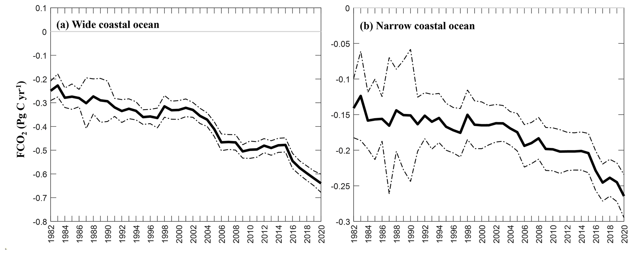
Figure 7Evolution of the global coastal CO2 sink (FCO2, in Pg C yr−1) over time using the reconstructed coastal pCO2-product (solid black line) with its associated uncertainties (dash-dotted black line; see Sects. 2.4 and 3.4 for further details). We use a 300 km distance from the coast as the outer limit of the coastal domain (wide coastal ocean) in (a) and the shelf break as the outer limit of the coastal domain (narrow coastal ocean) in (b).
Globally integrated, our results indicate that today's coastal ocean has been acting as a CO2 sink since the beginning of our study period (1982) both in the wide coastal ocean (Fig. 7a) and in the narrow domain (Fig. 7b). For both domains this CO2 sink, however, increases over time. In the wide coastal ocean, the global CO2 uptake amounted to 0.28 Pg C yr−1 in the 1980s (median value over the 1982–1992 period) and reached 0.54 Pg C yr−1 in the 2010s (mean value over the 2010–2020 period) with small interannual fluctuations (∼ 0.01 Pg C yr−1) of the CO2 sink intensity diagnosed by our algorithm. The overall intensification of the coastal sink that we observed in this study (0.06 Pg C yr−1 decade−1 (± 0.0009 Pg C yr−1 decade−1 with a p value <0.05) and 0.02 Pg C yr−1 decade−1 (± 0.0005 Pg C yr−1 decade−1 with a p value <0.05) for the wide and narrow coastal domain, respectively) supports the only two available observational coastal studies performed at the global scale (i.e., Laruelle et al., 2018; Wang et al., 2017) which were, however, significantly limited by the small fraction of the coastal ocean domain investigated (e.g., 6 % in Laruelle et al., 2018), and both predict an increase in efficiency of the global coastal CO2 sink over the past three decades. Our results are also in agreement with the conceptual approach of Bauer et al. (2013) as well as modeling studies, either using box models (e.g., Mackenzie et al., 2004, 2012; Rabouille et al., 2001; Ver et al., 1999) or, more recently, global ocean biogeochemical models (Bourgeois et al., 2016; Lacroix et al., 2021a, b) that all predict an increase in efficiency of the global coastal CO2 sink at the century scale.
The significant strengthening of this global coastal sink that we observed in this study has approximately doubled between 1982 and 2020 (wide coastal domain) and results from a general tendency towards an increase in the coastal CO2 sink intensities (e.g., in the high latitude of the Northern Hemisphere; Fig. 6a) combined with decreases in intensity of several CO2 sources such as along upwelling currents (e.g., in the Arabian Sea). However, since a large fraction of the global CO2 uptake results from coastal regions >40∘ of the Northern Hemisphere, and since these CO2 sink regions present strong negative rates of change in FCO2 (Fig. 6a), our results suggest that the primary driver of this 2-fold increase in the global coastal CO2 sink is to be found in the high latitudes of the Northern Hemisphere which contribute disproportionately to the global scale coastal FCO2 trend. Further studies should, however, be carried out to support this conclusion, given the paucity of observational pCO2 data in those high latitude regions that translate into high uncertainties in our pCO2-product, as for example in the Arctic Ocean. Taking also the large heterogeneity in the long-term FCO2 trends, a quantitative analysis of the respective contributions of different coastal systems to the global strengthening of the coastal CO2 sink should also be performed in the future, using a regionalized approach. Moreover, changes in wind speed and sea-ice coverage have likely not been constant over time, and further analysis of their influence on the rate change of FCO2 should be analyzed for each decade individually to better understand the interplay between these different drivers. Overall, our results highlight the complex nature of the coastal FCO2 dynamics and emphasize the need for further investigation and understanding of the specific factors influencing the FCO2 trends in different coastal regions.
Table 3Global FCO2 and pCO2 uncertainties calculated for the reconstructed data products using a wide delimitation and a narrow delimitation (given in parentheses) of the coastal domain.
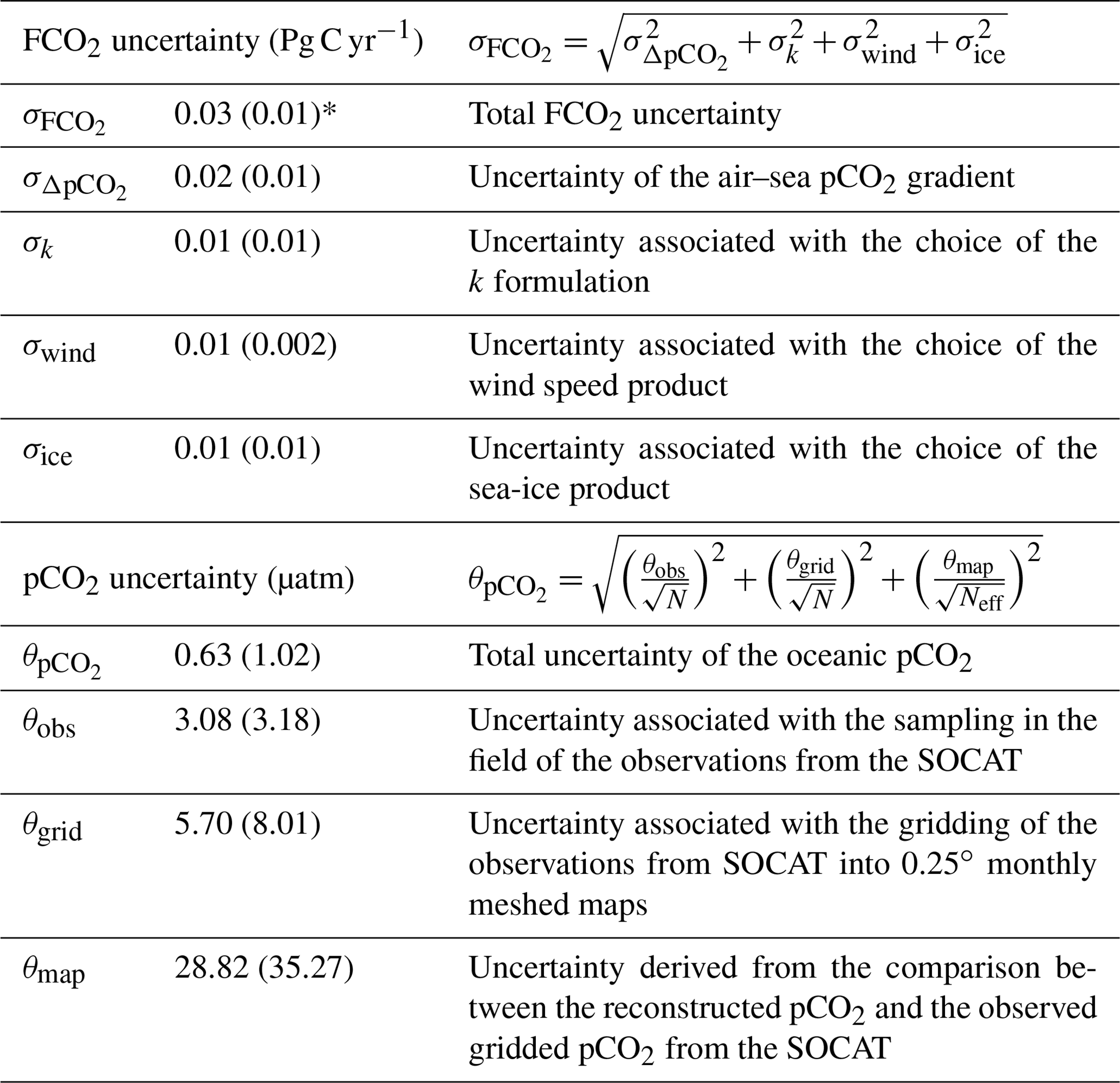
* The numbers correspond to uncertainties calculated using a wide coastal delimitation, while those enclosed in brackets represent uncertainties calculated using a narrow coastal delimitation.
3.4 Uncertainties associated with the data products
The global coastal CO2 sink of −0.40 Pg C yr−1 (wide coastal domain) that we calculate in this study using the ULB–SOM–FFN–coastalv2 pCO2-product is associated with a relative uncertainty that amounts to ∼10 % (value of 0.03 Pg C yr−1 for ; see Eq. 2 and Table 3). This global uncertainty mainly results from the uncertainty associated with the oceanic pCO2 (, uncertainty of 0.02 Pg C yr−1). The choice of the gas exchange transfer velocity formulation yields a 7 % difference (σk, uncertainty of 0.01 Pg C yr−1) on the global FCO2 calculation, whereas we calculate a ∼4 % difference on FCO2 depending on the wind speed product choice (σwind, uncertainty of 0.01 Pg C yr−1) or on the sea-ice product choice (σice, uncertainty of 0.01 Pg C yr−1) on the global FCO2 calculation. It is noteworthy, though, that the uncertainty in the mean is substantially lower than that calculated for individual months (see Fig. 7) or regions (e.g., see discussion above regarding the Baltic Sea region) due to compensating errors as was also identified in a study by Gloege et al. (2022).
The total uncertainty of the oceanic pCO2 (, value of 0.63 µatm; see Eq. 3) mainly results from the SOM–FFN mapping method to reconstruct the coastal pCO2-product (θmap=28.82 µatm; Table 3). This uncertainty falls within the range of values reported in the literature from different statistical interpolation methods to generate coastal pCO2 data products (RMSE values generally between 10 and 35 µatm; see Chen et al., 2016) which are calculated from regional studies and would be expected to be smaller than those calculated for global scale analysis (or even the performance of our algorithm at the scale of its provinces, which generally cover a much larger surface area than most regional studies). The θmap uncertainty calculated in this study is, however, higher than reported for the open ocean (typical RMSE values <20 µatm; e.g., Landschützer et al., 2014), mainly because of the complex biogeochemical dynamics and larger variability observed in the coastal seas compared with the open ocean. We calculate a global value of 3.08 µatm for θobs, the uncertainty on the sampling in the field of the observations from the SOCAT database, which is slightly higher than the value reported by Pfeil et al. (2013; value of 2 µatm). For θgrid, the uncertainty associated with the meshing of the observations from SOCAT to gridded 0.25∘ monthly maps, we calculate a global mean value of 5.70 µatm, which is close to the value reported by Sabine et al. (2013; 5 µatm) for the open ocean. It should be noted that all these uncertainties are calculated globally and can be larger at the regional scale (e.g., see Roobaert et al., 2019) as exemplified by the uncertainty associated with the choice of wind speed product on the FCO2 calculation (see Roobaert et al., 2018). Moreover, due to the temporal heterogeneity of the data coverage in the SOCAT database, our FCO2 uncertainties can also vary temporally. As shown in Fig. 7, the global FCO2 uncertainties that we report for each year (dash-dotted black lines) are largest in the 1980s (e.g., global value of 0.11 Pg C yr−1 in 1987) because of the scarcity of pCO2 measurements before 1990 in the SOCAT database and decrease over time. Our global uncertainties are also slightly larger along the nearshore domain of the coastal ocean. Using the narrow definition of the coastal domain (i.e., the shelf break as the outer limit), we calculate a global value of 0.01 Pg C yr−1 for (7 % uncertainty on the global FCO2, which is consistent with the global FCO2 uncertainty calculated by Roobaert et al. (2019; 10 %)). A 7 %, 2 % and 8 % FCO2 differences are calculated depend on the k formulation used (σk value of 0.01), the wind product choice (σwind=0.002 Pg C yr−1) and the sea-ice choice (σice=0.01 Pg C yr−1), respectively with the narrow coastal domain. For θmap, θgrid and θobs, we calculate values of 35 µatm, 8 µatm and 3 µatm, respectively.
The ULB–SOM–FFN–coastalv2 pCO2- and FCO2-products can be found at https://doi.org/10.25921/4sde-p068 (Roobaert et al., 2023). The bathymetry is derived from the 2 min global ETOPO2 database (Table 1; US Department of Commerce, 2006), the Chl a from the monthly 4 km merged GlobColour product for the 1998–2020 period from the EU Copernicus Marine Service information (https://doi.org/10.48670/moi-00281, Copernicus Marine Service, 2023), the SST and SSS from the daily NOAA OI SST V2 (Reynolds et al., 2007) and from the daily Hadley center EN4 SSS (Good et al., 2013), respectively. We use the atmospheric pCO2-product from the SeaFlux product (Fay et al., 2021) which is calculated from the dry air mixing ratio of CO2 (xCO2) provided by the ESRL surface marine boundary layer CO2 product (Dlugokencky et al., 2019; https://www.esrl.noaa.gov/gmd/ccgg/mbl/data.php) with a vapor correction according to Dickson et al. (2007) and using the ERA5 sea level pressure (Hersbach et al., 2023; https://doi.org/10.24381/cds.f17050d7). The sea-ice coverage is derived from the monthly mean of the daily 0.25∘ dataset of Reynolds et al. (2007) and the wind speed from the 6 h first moment of the 0.25∘ resolution product of the European Centre for Medium-Range Weather Forecasts (ECMWF) ERA5 (Hersbach et al., 2023). The pCO2 observations are derived from the SOCAT database v2022 (Bakker et al., 2022). The wind speed is calculated from the monthly mean of the 0.25∘ resolution product of the ECMWF ERA5 wind product (https://doi.org/10.24381/cds.f17050d7; Hersbach et al., 2023), which has a native temporal resolution of 6 h.
The release of the global coastal pCO2-product in 2017 by Laruelle et al. (2017) was a significant step forward for the investigation of the spatial distribution of CO2 sources and sinks as well as their seasonal variabilities in the shallow portion of the ocean. It was also instrumental to the completion and harmonization of global ocean air–sea CO2 fluxes (Fay et al., 2021), hence supporting global carbon budget analyses (Friedlingstein et al., 2022). However, this product was not designed or evaluated regarding its ability to resolve the interannual and decadal variabilities and the long-term evolution of the coastal air–sea CO2 exchange, which are still poorly understood (e.g., Bauer et al., 2013; Lacroix et al., 2021a; Laruelle et al., 2018; Regnier et al., 2013, 2022; Resplandy et al., 2023; Wang et al., 2017). In this study, we presented a new coastal pCO2-product for the 1982–2020 period using ∼18 million direct coastal observations from the SOCATv2022 database (Bakker et al., 2022) combined with an updated version of the coastal two-step SOM and FFN method used by Laruelle et al. (2017). We also provided a new coastal air–sea CO2 exchange product for the same period and examined the long-term trends, that is, the temporal evolution of the global coastal CO2 sink over the past four decades. This analysis reveals that the long-term trend of the air–sea pCO2 gradient drives most of the long-term evolution of the coastal CO2 sink, wind speed and sea-ice coverage playing a significant role regionally. Trend analysis of the coastal FCO2 has also been attempted using global ocean pCO2-products that cover the coastal domain (Resplandy et al., 2023). However, these investigations have been inconclusive, likely because global ocean pCO2-products cannot yet sufficiently well capture the specific and changing conditions occurring along the coastal domain (e.g., Chau et al, 2022; Rödenbeck et al., 2013; see also Resplandy et al., 2023). Our updated coastal pCO2-product circumvents these limitations and provides a first robust assessment against which outputs from global oceanic modes results can be evaluated (e.g., Resplandy et al., 2023). It will thus help better constrain the anthropogenic perturbation of the global ocean carbon cycle. In the future, our machine learning approach could also be used to diagnose the main drivers of change in the global coastal ocean sink and, more specifically, changes in the long-term trend evolution of the coastal pCO2 field. This approach, in conjunction with process-based simulations, is critically needed to evaluate and mitigate the impact of multiple anthropogenic perturbations (e.g., atmospheric pCO2 increase, physical climate, eutrophication and hypoxia) on the global coastal carbon cycle and associated biodiversity loss and other marine stressors.
The supplement related to this article is available online at: https://doi.org/10.5194/essd-16-421-2024-supplement.
AR and GGL designed the study. AR prepared the manuscript with contributions from all co-authors.
The contact author has declared that none of the authors has any competing interests.
Publisher's note: Copernicus Publications remains neutral with regard to jurisdictional claims made in the text, published maps, institutional affiliations, or any other geographical representation in this paper. While Copernicus Publications makes every effort to include appropriate place names, the final responsibility lies with the authors.
Goulven G. Laruelle is research associate of the F.R.S-FNRS at the Université Libre de Bruxelles. We thank one anonymous reviewer and Zelun Wu for their constructive comments and the editor for handling the manuscript.
This research has been supported by the European Union's Horizon 2020 research and innovation program (grant no. 101003536 (ESM2025 – Earth System Models for the Future)) and BELSPO (project ReCAP funded under the FEd-tWIN program). This paper was published in an open access format thanks to the support of the VLIZ Open Access budget.
This paper was edited by Xingchen Wang and reviewed by Laique Merlin Djeutchouang and one anonymous referee.
Atlas, R., Hoffman, R. N., Ardizzone, J., Leidner, S. M., Jusem, J. C., Smith, D. K., and Gombos, D.: A cross-calibrated, multiplatform ocean surface wind velocity product for meteorological and oceanographic applications, B. Am. Meteorol. Soc., 92, 157–174, https://doi.org/10.1175/2010BAMS2946.1, 2011.
Bai, Y., Cai, W. J., He, X., Zhai, W., Pan, D., Dai, M., and Yu, P.: A mechanistic semi-analytical method for remotely sensing sea surface pCO2 in river-dominated coastal oceans: A case study from the East China Sea, J. Geophys. Res.-Oceans, 120, 2331–2349, https://doi.org/10.1002/2014JC010632, 2015.
Bakker, D. C. E., Pfeil, B., Smith, K., Hankin, S., Olsen, A., Alin, S. R., Cosca, C., Harasawa, S., Kozyr, A., Nojiri, Y., O'Brien, K. M., Schuster, U., Telszewski, M., Tilbrook, B., Wada, C., Akl, J., Barbero, L., Bates, N. R., Boutin, J., Bozec, Y., Cai, W.-J., Castle, R. D., Chavez, F. P., Chen, L., Chierici, M., Currie, K., de Baar, H. J. W., Evans, W., Feely, R. A., Fransson, A., Gao, Z., Hales, B., Hardman-Mountford, N. J., Hoppema, M., Huang, W.-J., Hunt, C. W., Huss, B., Ichikawa, T., Johannessen, T., Jones, E. M., Jones, S. D., Jutterström, S., Kitidis, V., Körtzinger, A., Landschützer, P., Lauvset, S. K., Lefèvre, N., Manke, A. B., Mathis, J. T., Merlivat, L., Metzl, N., Murata, A., Newberger, T., Omar, A. M., Ono, T., Park, G.-H., Paterson, K., Pierrot, D., Ríos, A. F., Sabine, C. L., Saito, S., Salisbury, J., Sarma, V. V. S. S., Schlitzer, R., Sieger, R., Skjelvan, I., Steinhoff, T., Sullivan, K. F., Sun, H., Sutton, A. J., Suzuki, T., Sweeney, C., Takahashi, T., Tjiputra, J., Tsurushima, N., van Heuven, S. M. A. C., Vandemark, D., Vlahos, P., Wallace, D. W. R., Wanninkhof, R., and Watson, A. J.: An update to the Surface Ocean CO2 Atlas (SOCAT version 2), Earth Syst. Sci. Data, 6, 69–90, https://doi.org/10.5194/essd-6-69-2014, 2014.
Bakker, D. C., Alin, S. R., Becker, M., Bittig, H. C., Castaño-Primo, R., Feely, R. A., Gkritzalis, T., Kadono, K., Kozyr, A., Lauvset, S. K., Metzl, N., Munro, D. R., Nakaoka, S., Nojiri, Y., O'Brien, K. M., Olsen, A., Pfeil, B., Pierrot, D., Steinhoff, T., Sullivan, K. F., Sutton, A. J., Sweeney, C., Tilbrook, B., Wada, C., Wanninkhof, R., Willstrand Wranne, A., Akl, J., Apelthun, L. B., Bates, N., Beatty, C. M., Burger, E. F., Cai, W.-J., Cosca, C. E., Corredor, J. E., Cronin, M., Cross, J. N., De Carlo, E. H., DeGrandpre, M. D., Emerson, S. R., Enright, M. P., Enyo, K., Evans, W., Frangoulis, C., Fransson, A., García-Ibáñez, M. I., Gehrung, M., Giannoudi, L., Glockzin, M., Hales, B., Howden, S. D., Hunt, C. W., Ibánhez, J. S. P., Jones, S. D., Kamb, L., Körtzinger, A., Landa, C. S., Landschützer, P., Lefèvre, N., Lo Monaco, C., Macovei, V. A., Maenner Jones, S., Meinig, C., Millero, F. J., Monacci, N. M., Mordy, C., Morell, J. M., Murata, A., Musielewicz, S., Neill, C., Newberger, T., Nomura, D., Ohman, M., Ono, T., Passmore, A., Petersen, W., Petihakis, G., Perivoliotis, L., Plueddemann, A. J., Rehder, G., Reynaud, T., Rodriguez, C., Ross, A. C., Rutgersson, A., Sabine, C. L., Salisbury, J. E., Schlitzer, R., Send, U., Skjelvan, I., Stamataki, N., Sutherland, S. C., Sweeney, C., Tadokoro, K., Tanhua, T., Telszewski, M., Trull, T., Vandemark, D., van Ooijen, E., Voynova, Y. G., Wang, H., Weller, R. A., Whitehead, C., and Wilson, D.: Surface Ocean CO2 Atlas Database Version 2022 (SOCATv2022), NCEI Accession 0253659, NOAA National Centers for Environmental Information [data set], https://doi.org/10.25921/1h9f-nb73, 2022.
Bauer, J. E., Cai, W., Raymond, P. A., Bianchi, T. S., Hopkinson, C. S., and Regnier, P. : The changing carbon cycle of the coastal ocean, Nature, 504, 61, https://doi.org/10.1038/nature12857, 2013.
Becker, M., Olsen, A., Landschützer, P., Omar, A., Rehder, G., Rödenbeck, C., and Skjelvan, I.: The northern European shelf as an increasing net sink for CO2, Biogeosciences, 18, 1127–1147, https://doi.org/10.5194/bg-18-1127-2021, 2021.
Borges, A. V.: Do we have enough pieces of the jigsaw to integrate CO2 fluxes in the coastal ocean?, Estuaries, 28, 3–27, https://doi.org/10.1007/BF02732750, 2005.
Borges, A. V., Delille, B., and Frankignoulle, M.: Budgeting sinks and sources of CO2 in the coastal ocean: Diversity of ecosystem counts, Geophys. Res. Lett., 32, 1–4, https://doi.org/10.1029/2005GL023053, 2005.
Bourgeois, T., Orr, J. C., Resplandy, L., Terhaar, J., Ethé, C., Gehlen, M., and Bopp, L.: Coastal-ocean uptake of anthropogenic carbon, Biogeosciences, 13, 4167–4185, https://doi.org/10.5194/bg-13-4167-2016, 2016.
Cai, W.: Estuarine and Coastal Ocean Carbon Paradox: CO2 Sinks or Sites of Terrestrial Carbon Incineration?, Annu. Rev. Marine Sci., 3, 123–145, https://doi.org/10.1146/annurev-marine-120709-142723, 2011.
Cao, Z., Yang, W., Zhao, Y., Guo, X., Yin, Z., Du, C., Zhao, H., and Dai, M.: Diagnosis of CO2 dynamics and fluxes in global coastal oceans, National Sci. Rev., 7, 786–797, https://doi.org/10.1093/NSR/NWZ105, 2020.
Chau, T. T. T., Gehlen, M., and Chevallier, F.: A seamless ensemble-based reconstruction of surface ocean pCO2 and air–sea CO2 fluxes over the global coastal and open oceans, Biogeosciences, 19, 1087–1109, https://doi.org/10.5194/bg-19-1087-2022, 2022.
Chau, T.-T.-T., Gehlen, M., Metzl, N., and Chevallier, F.: CMEMS-LSCE: A global 0.25-degree, monthly reconstruction of the surface ocean carbonate system, Earth Syst. Sci. Data Discuss. [preprint], https://doi.org/10.5194/essd-2023-146, in review, 2023.
Chen, C.-T. A., Huang, T.-H., Chen, Y.-C., Bai, Y., He, X., and Kang, Y.: Air–sea exchanges of CO2 in the world's coastal seas, Biogeosciences, 10, 6509–6544, https://doi.org/10.5194/bg-10-6509-2013, 2013.
Chen, S., Hu, C., Byrne, R. H., Robbins, L. L., and Yang, B.: Remote estimation of surface pCO2 on the West Florida Shelf, Cont. Shelf Res., 128, 10–25, https://doi.org/10.1016/j.csr.2016.09.004, 2016.
Copernicus Marine Service: Global Ocean Colour (Copernicus-GlobColour), Bio-Geo-Chemical, L4 (monthly and interpolated) from Satellite Observations (1997–ongoing), Copernicus Marine Service [data set], https://doi.org/10.48670/moi-00281, 2023.
Dai, M., Su, J., Zhao, Y., Hofmann, E. E., Cao, Z., Cai, W., Gan, J., Lacroix, F., Laruelle, G. G., Meng, F., Müller, J. D., Regnier, P., Wang, G., and Wang, Z.: Carbon Fluxes in the Coastal Ocean: Synthesis, Boundary Processes and Future Trends, Annu. Rev. Earth Planet. Sci., 50, 593–626, https://doi.org/10.1146/annurev-earth-032320-090746, 2022.
Dickson, A. G., Sabine, C. L., and Christian, J. R.: Guide to best practices for ocean CO2 measurements, PICES Special Publication 3, 3, 191, https://doi.org/10.1159/000331784, 2007.
Dlugokencky, E. J., Thoning, K. W., Lang, P. M., and Tans, P. P.: NOAA Greenhouse Gas Reference from Atmospheric Carbon Dioxide Dry Air Mole Fractions from the NOAA ESRL Carbon Cycle Cooperative, Global Air Sampling Network [data set], https://www.esrl.noaa.gov/gmd/ccgg/mbl/data.php (last access: October 2023), 2019.
Eldering, A., Wennberg, P. O., Crisp, D., Schimel, D. S., Gunson, M. R., Chatterjee, A., Liu, J., Schwandner, F. M., Sun, Y., O'Dell, C. W., Frankenberg, C., Taylor, T., Fisher, B., Osterman, G. B., Wunch, D., Hakkarainen, J., Tamminen, J., and Weir, B.: The Orbiting Carbon Observatory-2 early science investigations of regional carbon dioxide fluxes, Science, 358, eaam5745, https://doi.org/10.1126/science.aam5745, 2017.
Fay, A. R., Gregor, L., Landschützer, P., McKinley, G. A., Gruber, N., Gehlen, M., Iida, Y., Laruelle, G. G., Rödenbeck, C., Roobaert, A., and Zeng, J.: SeaFlux: harmonization of air–sea CO2 fluxes from surface pCO2 data products using a standardized approach, Earth Syst. Sci. Data, 13, 4693–4710, https://doi.org/10.5194/essd-13-4693-2021, 2021.
Friedlingstein, P., Jones, M. W., O'Sullivan, M., Andrew, R. M., Bakker, D. C. E., Hauck, J., Le Quéré, C., Peters, G. P., Peters, W., Pongratz, J., Sitch, S., Canadell, J. G., Ciais, P., Jackson, R. B., Alin, S. R., Anthoni, P., Bates, N. R., Becker, M., Bellouin, N., Bopp, L., Chau, T. T. T., Chevallier, F., Chini, L. P., Cronin, M., Currie, K. I., Decharme, B., Djeutchouang, L. M., Dou, X., Evans, W., Feely, R. A., Feng, L., Gasser, T., Gilfillan, D., Gkritzalis, T., Grassi, G., Gregor, L., Gruber, N., Gürses, Ö., Harris, I., Houghton, R. A., Hurtt, G. C., Iida, Y., Ilyina, T., Luijkx, I. T., Jain, A., Jones, S. D., Kato, E., Kennedy, D., Klein Goldewijk, K., Knauer, J., Korsbakken, J. I., Körtzinger, A., Landschützer, P., Lauvset, S. K., Lefèvre, N., Lienert, S., Liu, J., Marland, G., McGuire, P. C., Melton, J. R., Munro, D. R., Nabel, J. E. M. S., Nakaoka, S.-I., Niwa, Y., Ono, T., Pierrot, D., Poulter, B., Rehder, G., Resplandy, L., Robertson, E., Rödenbeck, C., Rosan, T. M., Schwinger, J., Schwingshackl, C., Séférian, R., Sutton, A. J., Sweeney, C., Tanhua, T., Tans, P. P., Tian, H., Tilbrook, B., Tubiello, F., van der Werf, G. R., Vuichard, N., Wada, C., Wanninkhof, R., Watson, A. J., Willis, D., Wiltshire, A. J., Yuan, W., Yue, C., Yue, X., Zaehle, S., and Zeng, J.: Global Carbon Budget 2021, Earth Syst. Sci. Data, 14, 1917–2005, https://doi.org/10.5194/essd-14-1917-2022, 2022.
Gloege, L., Yan, M., Zheng, T., and McKinley, G. A.: Improved Quantification of Ocean Carbon Uptake by Using Machine Learning to Merge Global Models and pCO2 Data, J. Adv. Model. Earth Syst., 14, e2021MS002620, https://doi.org/10.1029/2021MS002620, 2022.
Good, S. A., Martin, M. J., and Rayner, N. A.: EN4: Quality controlled ocean temperature and salinity profiles and monthly objective analyses with uncertainty estimates, J. Geophys. Res.-Oceans, 118, 6704–6716, https://doi.org/10.1002/2013JC009067, 2013.
Gregor, L. and Gruber, N.: OceanSODA-ETHZ: a global gridded data set of the surface ocean carbonate system for seasonal to decadal studies of ocean acidification, Earth Syst. Sci. Data, 13, 777–808, https://doi.org/10.5194/essd-13-777-2021, 2021.
Hales, B., Strutton, P. G., Saraceno, M., Letelier, R., Takahashi, T., Feely, R., Sabine, C., and Chavez, F.: Satellite-based prediction of pCO2 in coastal waters of the eastern North Pacific, Prog. Oceanogr., 103, 1–15, https://doi.org/10.1016/j.pocean.2012.03.001, 2012.
Hauck, J., Zeising, M., Le Quéré, C., Gruber, N., Bakker, D. C. E., Bopp, L., Chau, T. T. T., Gürses, Ö., Ilyina, T., Landschützer, P., Lenton, A., Resplandy, L., Rödenbeck, C., Schwinger, J., and Séférian, R.: Consistency and Challenges in the Ocean Carbon Sink Estimate for the Global Carbon Budget, Front. Marine Sci., 7, 571720, https://doi.org/10.3389/fmars.2020.571720, 2020.
Hersbach, H., Bell, B., Berrisford, P., Biavati, G., Horányi, A., Muñoz Sabater, J., Nicolas, J., Peubey, C., Radu, R., Rozum, I., Schepers, D., Simmons, A., Soci, C., Dee, D., and Thépaut, J.-N.: ERA5 monthly averaged data on single levels from 1940 to present, Copernicus Climate Change Service (C3S) Climate Data Store (CDS) [data set], https://doi.org/10.24381/cds.f17050d7, 2023.
Ho, D. T., Wanninkhof, R., Schlosser, P., Ullman, D. S., Hebert, D., and Sullivan, K. F.: Toward a universal relationship between wind speed and gas exchange: Gas transfer velocities measured with 3He/SF6 during the Southern Ocean Gas Exchange Experiment, J. Geophys. Res.-Oceans, 116, C00F04, https://doi.org/10.1029/2010JC006854, 2011.
Iida, Y., Kojima, A., Takatani, Y., Nakano, T., Sugimoto, H., Midorikawa, T., and Ishii, M.: Trends in pCO2 and sea–air CO2 flux over the global open oceans for the last two decades, J. Oceanogr., 71, 637–661, https://doi.org/10.1007/s10872-015-0306-4, 2015.
Jamet, C., Moulin, C., and Lefèvre, N.: Estimation of the oceanic pCO2 in the North Atlantic from VOS lines in-situ measurements: parameters needed to generate seasonally mean maps, Ann. Geophys., 25, 2247–2257, https://doi.org/10.5194/angeo-25-2247-2007, 2007.
Jones, S. D., Le Quéré, C., Rödenbeck, C., Manning, A. C., and Olsen, A.: A statistical gap-filling method to interpolate global monthly surface ocean carbon dioxide data, J. Adv. Model. Earth Syst., 7, 1554–1575, https://doi.org/10.1002/2014MS000416, 2015.
Kalnay, E., Kanamitsu, M., Kistler, R., Collins, W., Deaven, D., Gandin, L., Iredell, M., Saha, S., White, G., Woollen, J., Zhu, Y., Chelliah, M., Ebisuzaki, W., Higgins, W., Janowiak, J., Mo, K. C., Ropelewski, C., Wang, J., Leetmaa, A., Reynolds, R., Jenne, R., and Joseph, D.: The NCEP/NCAR 40-year reanalysis project, B. Am. Meteorol. Soc., 77, 437–471, https://doi.org/10.1175/1520-0477(1996)077<0437:TNYRP>2.0.CO;2, 1996.
Lacroix, F., Ilyina, T., Laruelle, G. G., and Regnier, P.: Reconstructing the Preindustrial Coastal Carbon Cycle Through a Global Ocean Circulation Model: Was the Global Continental Shelf Already Both Autotrophic and a CO2 Sink?, Global Biogeochem. Cycles, 35, e2020GB006603, https://doi.org/10.1029/2020GB006603, 2021a.
Lacroix, F., Ilyina, T., Mathis, M., Laruelle, G. G., and Regnier, P.: Historical increases in land-derived nutrient inputs may alleviate effects of a changing physical climate on the oceanic carbon cycle, Global Change Biol., 27, 5491–5513, https://doi.org/10.1111/gcb.15822, 2021b.
Landschützer, P., Gruber, N., Bakker, D. C. E., Schuster, U., Nakaoka, S., Payne, M. R., Sasse, T. P., and Zeng, J.: A neural network-based estimate of the seasonal to inter-annual variability of the Atlantic Ocean carbon sink, Biogeosciences, 10, 7793–7815, https://doi.org/10.5194/bg-10-7793-2013, 2013.
Landschützer, P., Gruber, N., Bakker, D. C. E., and Schuster, U.: Recent variability of the global ocean carbon sink, Global Biogeochem. Cycles, 28, 927–949, https://doi.org/10.1002/2014GB004853, 2014.
Landschützer, P., Gruber, N., and Bakker, D. C. E.: Decadal variations and trends of the global ocean carbon sink, Global Biogeochem. Cycles, 30, 1396–1417, https://doi.org/10.1002/2015GB005359, 2016.
Landschützer, P., Gruber, N., Bakker, D. C. E., Stemmler, I., and Six, K. D.: Strengthening seasonal marine CO2 variations due to increasing atmospheric CO2, Nat. Clim. Change, 8, 146–150, https://doi.org/10.1038/s41558-017-0057-x, 2018.
Landschützer, P., Laruelle, G. G., Roobaert, A., and Regnier, P.: A uniform pCO2 climatology combining open and coastal oceans, Earth Syst. Sci. Data, 12, 2537–2553, https://doi.org/10.5194/essd-12-2537-2020, 2020.
Laruelle, G. G., Dürr, H. H., Slomp, C. P., and Borges, A. V.: Evaluation of sinks and sources of CO2 in the global coastal ocean using a spatially-explicit typology of estuaries and continental shelves, Geophys. Res. Lett., 37, 1–6, https://doi.org/10.1029/2010GL043691, 2010.
Laruelle, G. G., Dürr, H. H., Lauerwald, R., Hartmann, J., Slomp, C. P., Goossens, N., and Regnier, P. A. G.: Global multi-scale segmentation of continental and coastal waters from the watersheds to the continental margins, Hydrol. Earth Syst. Sci., 17, 2029–2051, https://doi.org/10.5194/hess-17-2029-2013, 2013.
Laruelle, G. G., Lauerwald, R., Pfeil, B., and Regnier, P.: Regionalized global budget of the CO2 exchange at the air-water interface in continental shelf seas, Global Biogeochem. Cycles, 28, 1199–1214, https://doi.org/10.1002/2014GB004832, 2014.
Laruelle, G. G., Landschützer, P., Gruber, N., Tison, J.-L., Delille, B., and Regnier, P.: Global high-resolution monthly pCO2 climatology for the coastal ocean derived from neural network interpolation, Biogeosciences, 14, 4545–4561, https://doi.org/10.5194/bg-14-4545-2017, 2017.
Laruelle, G. G., Cai, W.-J., Hu, X., Gruber, N., Mackenzie, F. T., and Regnier, P.: Continental shelves as a variable but increasing global sink for atmospheric carbon dioxide, Nat. Commun., 9, 454, https://doi.org/10.1038/s41467-017-02738-z, 2018.
Mackenzie, F. T., Lerman, A., and Andersson, A. J.: Past and present of sediment and carbon biogeochemical cycling models, Biogeosciences, 1, 11–32, https://doi.org/10.5194/bg-1-11-2004, 2004.
Mackenzie, F. T., De Carlo, E. H., and Lerman, A.: Coupled C, N, P, and O Biogeochemical Cycling at the Land-Ocean Interface, Elsevier Inc, 317–342 pp., https://doi.org/10.1016/B978-0-12-374711-2.00512-X, 2012.
Majkut, J. D., Sarmiento, J. L., and Rodgers, K. B.: A growing oceanic carbon uptake: Results from an inversion study of surface pCO2 data, Global Biogeochem. Cycles, 28, 335–351, https://doi.org/10.1002/2013GB004585, 2014.
Nakaoka, S., Telszewski, M., Nojiri, Y., Yasunaka, S., Miyazaki, C., Mukai, H., and Usui, N.: Estimating temporal and spatial variation of ocean surface pCO2 in the North Pacific using a self-organizing map neural network technique, Biogeosciences, 10, 6093–6106, https://doi.org/10.5194/bg-10-6093-2013, 2013.
Ono, T., Saino, T., Kurita, N., and Sasaki, K.: Basin-scale extrapolation of shipboard pCO2 data by using satellite SST and Chl a, Int. J. Remote Sens., 25, 3803–3815, https://doi.org/10.1080/01431160310001657515, 2004.
Park, G. H., Wanninkhof, R., Doney, S. C., Takahashi, T., Lee, K., Feely, R. A., Sabine, C. L., Trińlanes, J., and Lima, I. D.: Variability of global net sea-air CO2 fluxes over the last three decades using empirical relationships, Tellus B, 62, 352–368, https://doi.org/10.1111/j.1600-0889.2010.00498.x, 2010.
Pfeil, B., Olsen, A., Bakker, D. C. E., Hankin, S., Koyuk, H., Kozyr, A., Malczyk, J., Manke, A., Metzl, N., Sabine, C. L., Akl, J., Alin, S. R., Bates, N., Bellerby, R. G. J., Borges, A., Boutin, J., Brown, P. J., Cai, W.-J., Chavez, F. P., Chen, A., Cosca, C., Fassbender, A. J., Feely, R. A., González-Dávila, M., Goyet, C., Hales, B., Hardman-Mountford, N., Heinze, C., Hood, M., Hoppema, M., Hunt, C. W., Hydes, D., Ishii, M., Johannessen, T., Jones, S. D., Key, R. M., Körtzinger, A., Landschützer, P., Lauvset, S. K., Lefèvre, N., Lenton, A., Lourantou, A., Merlivat, L., Midorikawa, T., Mintrop, L., Miyazaki, C., Murata, A., Nakadate, A., Nakano, Y., Nakaoka, S., Nojiri, Y., Omar, A. M., Padin, X. A., Park, G.-H., Paterson, K., Perez, F. F., Pierrot, D., Poisson, A., Ríos, A. F., Santana-Casiano, J. M., Salisbury, J., Sarma, V. V. S. S., Schlitzer, R., Schneider, B., Schuster, U., Sieger, R., Skjelvan, I., Steinhoff, T., Suzuki, T., Takahashi, T., Tedesco, K., Telszewski, M., Thomas, H., Tilbrook, B., Tjiputra, J., Vandemark, D., Veness, T., Wanninkhof, R., Watson, A. J., Weiss, R., Wong, C. S., and Yoshikawa-Inoue, H.: A uniform, quality controlled Surface Ocean CO2 Atlas (SOCAT), Earth Syst. Sci. Data, 5, 125–143, https://doi.org/10.5194/essd-5-125-2013, 2013.
Rabouille, C., Mackenzie, F. T., and Ver, L. M.: Influence of the human perturbation on carbon, nitrogen, and oxygen biogeochemical cycles in the global coastal ocean, Geochim. Cosmochim. Ac., 65, 3615–3641, https://doi.org/10.1016/S0016-7037(01)00760-8, 2001.
Rayner, N. A., Parker, D. E., Horton, E. B., Folland, C. K., Alexander, L. V., Rowell, D. P., Kent, E. C., and Kaplan, A.: Global analyses of sea surface temperature, sea ice, and night marine air temperature since the late nineteenth century, J. Geophys. Res., 108, 4407, https://doi.org/10.1029/2002JD002670, 2003.
Regnier, P., Friedlingstein, P., Ciais, P., Mackenzie, F. T., Gruber, N., Janssens, I. A., Laruelle, G. G., Lauerwald, R., Luyssaert, S., Andersson, A. J., Arndt, S., Arnosti, C., Borges, A. V, Dale, A. W., Gallego-Sala, A., Goddéris, Y., Goossens, N., Hartmann, J., Heinze, C., Ilyina, T., Joos, F., LaRowe, D. E., Leifeld, J., Meysman, F. J. R., Munhoven, G., Raymond, P. A., Spahni, R., Suntharalingam, P., and Thullner, M.: Anthropogenic perturbation of the carbon fluxes from land to ocean, Nat. Geosci., 6, 597–607, https://doi.org/10.1038/ngeo1830, 2013.
Regnier, P., Resplandy, L., Najjar, R. G., and Ciais, P.: The land-to-ocean loops of the global carbon cycle, Nature, 603, 401–410, https://doi.org/10.1038/s41586-021-04339-9, 2022.
Resplandy, L., Hogikyan, A., Bange, H., Bianchi, D., Weber, T. S.,Cai, W.-J., Doney, S. C., Fennel, K., Gehlen, M., Hauck, J., Lacroix, F., Landschützer, P., Le Quéré, C., Müller, J. D., Najjar, R. G., Roobaert, A., Berthet, S., Bopp, L., Chau, T. T.-T., Dai, M., Gruber, N., Ilyina, T., Kock, A., Manizza, M., Lachkar, Z., Laruelle, G. G., Liao, E., Lima, I. D., Nissen, C., Rödenbeck, C., Séférian, R., Schwinger, J., Toyama, K., Tsujino, H., and Regnier, P.: A Synthesis of Global Coastal Ocean Greenhouse Gas Fluxes, ESS Open Archive, 18 April 2023, https://doi.org/10.22541/essoar.168182303.39621839/v1, 2023.
Reynolds, R. W., Smith, T. M., Liu, C., Chelton, D. B., Casey, K. S., and Schlax, M. G.: Daily high-resolution-blended analyses for sea surface temperature, J. Climate, 20, 5473–5496, https://doi.org/10.1175/2007JCLI1824.1, 2007.
Rödenbeck, C., Keeling, R. F., Bakker, D. C. E., Metzl, N., Olsen, A., Sabine, C., and Heimann, M.: Global surface-ocean pCO2 and sea–air CO2 flux variability from an observation-driven ocean mixed-layer scheme, Ocean Sci., 9, 193–216, https://doi.org/10.5194/os-9-193-2013, 2013.
Rödenbeck, C., Bakker, D. C. E., Metzl, N., Olsen, A., Sabine, C., Cassar, N., Reum, F., Keeling, R. F., and Heimann, M.: Interannual sea–air CO2 flux variability from an observation-driven ocean mixed-layer scheme, Biogeosciences, 11, 4599–4613, https://doi.org/10.5194/bg-11-4599-2014, 2014.
Rödenbeck, C., Bakker, D. C. E., Gruber, N., Iida, Y., Jacobson, A. R., Jones, S., Landschützer, P., Metzl, N., Nakaoka, S., Olsen, A., Park, G.-H., Peylin, P., Rodgers, K. B., Sasse, T. P., Schuster, U., Shutler, J. D., Valsala, V., Wanninkhof, R., and Zeng, J.: Data-based estimates of the ocean carbon sink variability – first results of the Surface Ocean pCO2 Mapping intercomparison (SOCOM), Biogeosciences, 12, 7251–7278, https://doi.org/10.5194/bg-12-7251-2015, 2015.
Roobaert, A., Laruelle, G. G., Landschützer, P., and Regnier, P.: Uncertainty in the global oceanic CO2 uptake induced by wind forcing: quantification and spatial analysis, Biogeosciences, 15, 1701–1720, https://doi.org/10.5194/bg-15-1701-2018, 2018.
Roobaert, A., Laruelle, G. G., Landschützer, P., Gruber, N., Chou, L., and Regnier, P.: The Spatiotemporal Dynamics of the Sources and Sinks of CO2 in the Global Coastal Ocean, Global Biogeochem. Cycles, 33, 1693–1714, https://doi.org/10.1029/2019GB006239, 2019.
Roobaert, A., Regnier, P., Landschützer, P., and Laruelle, G. G.: A novel sea surface partial pressure of carbon dioxide (pCO2) data product for the global coastal ocean resolving trends over the 1982–2020 period (NCEI Accession 0279118), NOAA National Centers for Environmental Information [data set], https://www.ncei.noaa.gov/archive/accession/0279118 (last access: 19 June 2023), 2023.
Sabine, C. L., Hankin, S., Koyuk, H., Bakker, D. C. E., Pfeil, B., Olsen, A., Metzl, N., Kozyr, A., Fassbender, A., Manke, A., Malczyk, J., Akl, J., Alin, S. R., Bellerby, R. G. J., Borges, A., Boutin, J., Brown, P. J., Cai, W.-J., Chavez, F. P., Chen, A., Cosca, C., Feely, R. A., González-Dávila, M., Goyet, C., Hardman-Mountford, N., Heinze, C., Hoppema, M., Hunt, C. W., Hydes, D., Ishii, M., Johannessen, T., Key, R. M., Körtzinger, A., Landschützer, P., Lauvset, S. K., Lefèvre, N., Lenton, A., Lourantou, A., Merlivat, L., Midorikawa, T., Mintrop, L., Miyazaki, C., Murata, A., Nakadate, A., Nakano, Y., Nakaoka, S., Nojiri, Y., Omar, A. M., Padin, X. A., Park, G.-H., Paterson, K., Perez, F. F., Pierrot, D., Poisson, A., Ríos, A. F., Salisbury, J., Santana-Casiano, J. M., Sarma, V. V. S. S., Schlitzer, R., Schneider, B., Schuster, U., Sieger, R., Skjelvan, I., Steinhoff, T., Suzuki, T., Takahashi, T., Tedesco, K., Telszewski, M., Thomas, H., Tilbrook, B., Vandemark, D., Veness, T., Watson, A. J., Weiss, R., Wong, C. S., and Yoshikawa-Inoue, H.: Surface Ocean CO2 Atlas (SOCAT) gridded data products, Earth Syst. Sci. Data, 5, 145–153, https://doi.org/10.5194/essd-5-145-2013, 2013.
Sarma, V. V. S. S., Saino, T., Sasaoka, K., Nojiri, Y., Ono, T., Ishii, M., Inoue, H. Y., and Matsumoto, K.: Basin-scale pCO2 distribution using satellite sea surface temperature, Chl a, and climatological salinity in the North Pacific in spring and summer, Global Biogeochem. Cycles, 20, GB3005, https://doi.org/10.1029/2005GB002594, 2006.
Schuster, U., McKinley, G. A., Bates, N., Chevallier, F., Doney, S. C., Fay, A. R., González-Dávila, M., Gruber, N., Jones, S., Krijnen, J., Landschützer, P., Lefèvre, N., Manizza, M., Mathis, J., Metzl, N., Olsen, A., Rios, A. F., Rödenbeck, C., Santana-Casiano, J. M., Takahashi, T., Wanninkhof, R., and Watson, A. J.: An assessment of the Atlantic and Arctic sea–air CO2 fluxes, 1990–2009, Biogeosciences, 10, 607–627, https://doi.org/10.5194/bg-10-607-2013, 2013.
Serreze, M. C. and Meier, W. N.: The Arctic's sea ice cover: trends, variability, predictability, and comparisons to the Antarctic, Ann. NY Acad. Sci., 1436, 36–53, https://doi.org/10.1111/nyas.13856, 2019.
Sharp, J. D., Fassbender, A. J., Carter, B. R., Lavin, P. D., and Sutton, A. J.: A monthly surface pCO2 product for the California Current Large Marine Ecosystem, Earth Syst. Sci. Data, 14, 2081–2108, https://doi.org/10.5194/essd-14-2081-2022, 2022.
Shutler, J. D., Land, P. E., Piolle, J. F., Woolf, D. K., Goddijn-Murphy, L., Paul, F., Girard-Ardhuin, F., Chapron, B., and Donlon, C. J.: FluxEngine: A flexible processing system for calculating atmosphere-ocean carbon dioxide gas fluxes and climatologies, J. Atmos. Ocean. Tech., 33, 741–756, https://doi.org/10.1175/JTECH-D-14-00204.1, 2016.
Sutton, A. J., Feely, R. A., Maenner-Jones, S., Musielwicz, S., Osborne, J., Dietrich, C., Monacci, N., Cross, J., Bott, R., Kozyr, A., Andersson, A. J., Bates, N. R., Cai, W.-J., Cronin, M. F., De Carlo, E. H., Hales, B., Howden, S. D., Lee, C. M., Manzello, D. P., McPhaden, M. J., Meléndez, M., Mickett, J. B., Newton, J. A., Noakes, S. E., Noh, J. H., Olafsdottir, S. R., Salisbury, J. E., Send, U., Trull, T. W., Vandemark, D. C., and Weller, R. A.: Autonomous seawater pCO2 and pH time series from 40 surface buoys and the emergence of anthropogenic trends, Earth Syst. Sci. Data, 11, 421–439, https://doi.org/10.5194/essd-11-421-2019, 2019.
Sweeney, C., Gloor, E., Jacobson, A. R., Key, R. M., McKinley, G. A., Sarmiento, J. L., and Wanninkhof, R.: Constraining global air-sea gas exchange for CO2 with recent bomb 14C measurements, Global Biogeochem. Cycles, 21, 1–10, https://doi.org/10.1029/2006GB002784, 2007.
Takahashi, T., Sutherland, S. C., Wanninkhof, R., Sweeney, C., Feely, R. A. R. A., Chipman, D. W. D. W., Hales, B., Friederich, G., Chavez, F., Sabine, C., Watson, A., Baker, D. F., Schuster, U., Metzl, N., Yoshikawa-Inoue, H., Ishii, M., Midorikawa, T., Nojiri, Y., Körtzinger, A., Steinhoff, T., Hoppema, M., Olafsson, J., Arnarson, T. S., Tilbrook, B., Johannessen, T., Olsen, A., Bellerby, R., Wong, C. S., Delille, B., Bates, N. R., and de Baar, H. J. W.: Climatological mean and decadal change in surface ocean pCO2, and net sea-air CO2 flux over the global oceans, Deep-Sea Res. Pt. II, 56, 554–577, https://doi.org/10.1016/j.dsr2.2008.12.009, 2009.
Takahashi, T., Sutherland, S. C., and Kozyr, A.: Global ocean surface water partial pressure of CO2 database: Measurements performed during 1957–2018 (version 2018), NOAA/NCEI/OCADS NDP-088 (V2018) Rep., 25 pp., https://www.ncei.noaa.gov/access/ocean-carbon-data-system/oceans/LDEO_Underway_Database/NDP-088_V2018.Pdf (last access: October 2023), 2019.
US Department of Commerce, National Oceanic and Atmospheric Administration, National Geophysical Data Center, 2-minute Gridded Global Relief Data (ETOPO2v2), http://www.ngdc.noaa.gov/mgg/fliers/06mgg01.html (last access: 26 December 2022), 2006.
Ver, L. M. B., Mackenzie, F. T., and Lerman, A.: Carbon cycle in the coastal zone: Effects of global perturbations and change in the past three centuries, Chem. Geol., 159, 283–304, https://doi.org/10.1016/S0009-2541(99)00042-X, 1999.
Wang, H., Hu, X., Cai, W. J., and Sterba-Boatwright, B.: Decadal fCO2 trends in global ocean margins and adjacent boundary current-influenced areas, Geophys. Res. Lett., 44, 8962–8970, https://doi.org/10.1002/2017GL074724, 2017.
Wanninkhof, R.: Relationship between wind speed and gas exchange over the ocean revisited, Limnol. Oceanogr.-Methods, 12, 351–362, https://doi.org/10.1029/92JC00188, 2014.
Weiss, R. F.: Carbon dioxide in water and seawater: the solubility of a non-ideal gas, Marine Chem., 2, 203–215, https://doi.org/10.1016/0304-4203(74)90015-2, 1974.
Wrobel-Niedzwiecka, I., Kitowska, M., Makuch, P., and Markuszewski, P.: The Distribution of pCO2W and Air-Sea CO2 Fluxes Using FFNN at the Continental Shelf Areas of the Arctic Ocean, Remote Sens., 14, 312, https://doi.org/10.3390/rs14020312, 2022.
Zeng, J., Nojiri, Y., Landschützer, P., Telszewski, M., and Nakaoka, S.: A global surface ocean fCO2 climatology based on a feed-forward neural network, J. Atmos. Ocean. Tech., 31, 1838–1849, https://doi.org/10.1175/JTECH-D-13-00137.1, 2014.