Multiwavelength aerosol lidars at the Maïdo supersite, Réunion Island, France: instrument description, data processing chain, and quality assessment

Understanding optical and radiative properties of aerosols and clouds is critical to reducing uncertainties in climate models. For over 10 years, the Observatory of Atmospheric Physics in Reunion (OPAR; 21.079° S, 55.383° E) has been operating three active lidar instruments, named lidar 1200 (Li1200), stratospheric ozone lidar (LiO3S), and tropospheric ozone lidar (LiO3T), providing time series of vertical profiles from 3 to 45 km of the aerosol extinction and backscatter coefficients at 355 and 532 nm as well as the linear depolarization ratio at 532 nm. This work provides a full technical description of the three systems, the details about the methods chosen for the signal preprocessing and processing, and an uncertainty analysis. About 1737 nighttime averaged profiles were manually screened to provide cloud-free and artifact-free profiles. Data processing consisted of Klett inversion to retrieve aerosol optical products from preprocessed files. The measurement frequency was lower during the wet season and the holiday periods. There is a good correlation between the Li1200 and LiO3S instruments in terms of stratospheric aerosol optical depth (AOD) at 355 nm (0.001–0.107; $R=\mathrm{0.92}\pm \mathrm{0.01}$) and with LiO3T in terms of Ångström exponent 355/532 (0.079–1.288; $R=\mathrm{0.90}\pm \mathrm{0.13}$). The lowest values of the averaged uncertainty in the aerosol backscatter coefficient for the three time series are 64.4 ± 31.6 % for LiO3S, 50.3 ± 29.0 % for Li1200, and 69.1 ± 42.7 % for LiO3T. These relative uncertainties are high for the three instruments because of the very low values of extinction and backscatter coefficients for background aerosols above Maïdo observatory. Uncertainty increases due to the signal-to-noise ratio (SNR) decrease above 25 km for LIO3S and Li1200 and above 20 km for LiO3T. The lidar ratio (LR) is responsible for an uncertainty increase below 18 km (10 km) for LiO3S and Li1200 (LiO3T). LiO3S is the most stable instrument at 355 nm due to fewer technical modifications and fewer misalignments. Li1200 is a valuable addition meant to fill in the gaps in the LiO3S time series at 355 nm or for specific case studies about the middle and low troposphere. Data described in this work are available at https://doi.org/10.26171/rwcm-q370 (Gantois et al., 2024).

1 Introduction

Uncertainties concerning aerosol and cloud optical and radiative properties strongly affect surface climate and also the accuracy in climate models (Hansen et al., 1997; Alexander et al., 2013). Aerosols can be of multiple origins, compositions, sizes, and shapes but can also interact at different temporal and spatial scales and be influenced by various dynamical processes. This makes their observation on the global scale and the modeling of their properties challenging. Improving our knowledge in this area implies the use of different measurement techniques (in situ, active, and passive remote sensing methods) synergistically and providing continuous time series of high-resolution measurements in the low and middle atmosphere.

The Observatory of Atmospheric Physics in Reunion (OPAR), located on Réunion Island near Madagascar, is currently equipped with more than 50 instruments distributed over three different sites: two historical coastal sites in the north and a high-altitude site (Maïdo observatory; 2160 m a.s.l., Baray et al., 2013), which now houses more than two-thirds of these instruments. OPAR is part of many international networks, including GAW (Global Atmosphere Watch Programme), NDACC (Network for the Detection of Atmospheric Composition Change), SHADOZ (Southern Hemisphere ADditional OZonesondes), and AERONET (Aerosol Robotic Network). Additionally, it is a part of the European research infrastructures ACTRIS (Aerosol, Clouds and Trace Gases Research Infrastructure) and ICOS (Integrated Carbon Observation System).

Maïdo observatory (21.079° S, 55.383° E) is one of the very few active observational sites in the Southern Hemisphere (SH). It is barely influenced by anthropic aerosols. Its importance lies in the fact that the aerosol load in the atmosphere above Réunion Island is under the influence of many different sources of emission and dynamical processes responsible for short- and long-range air-mass transports (Baray et al., 2013), such as biomass burning (BB) plumes (Edwards et al., 2006; Khaykin et al., 2020), which are seasonally emitted in the SH. Moreover, it is not rare for volcanic aerosols to be detected in the stratosphere above Maïdo observatory. In fact, several volcanoes are located at the same latitude (Hunga Tonga) or in the same hemisphere (Calbuco) as Réunion Island (Bègue et al., 2017; Khaykin et al., 2017; Tidiga et al., 2022; Baron et al., 2023; Sicard et al., 2024). The high altitude of this facility is also of great importance as it is located above the boundary layer during the night, allowing for the observation of the free troposphere in a quasi-pristine environment.

Since its creation in 2012, the Maïdo facility has been equipped with four research lidar (light detection and ranging) instruments emitting electromagnetic radiations at different wavelengths. Three of them have been providing high-resolution time series of aerosol extinction and backscatter vertical profiles in the UV (355 nm) and visible (532 nm) domains. As of today, these measurements have only been occasionally used for case studies (Bègue et al., 2017; Khaykin et al., 2017; Tidiga et al., 2022; Baron et al., 2023; Sicard et al., 2024). Full exploitation of these time series will make providing time series of aerosol extinction and backscatter profiles over Réunion Island possible. This can only be achieved after homogenizing the processing method for the three instruments.

This work provides a summary of the specifications of the systems and a full description of the preprocessing and processing methods used to produce different levels of the datasets for the three Maïdo lidars.

2 Instrument description

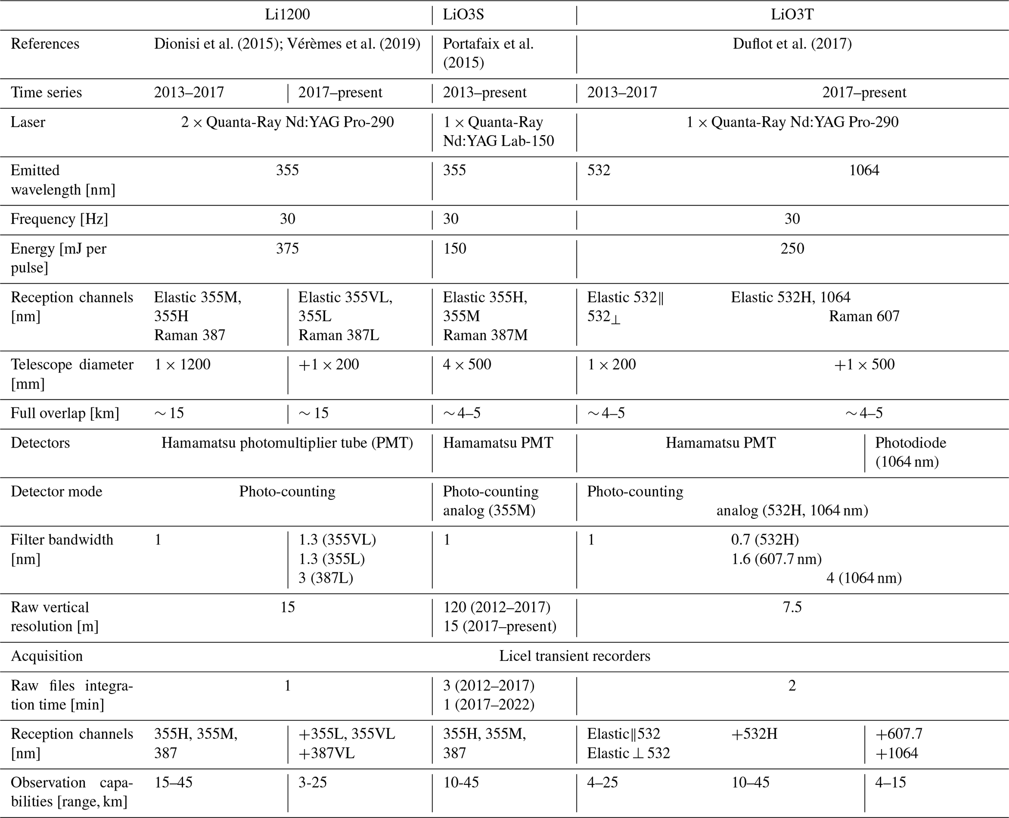
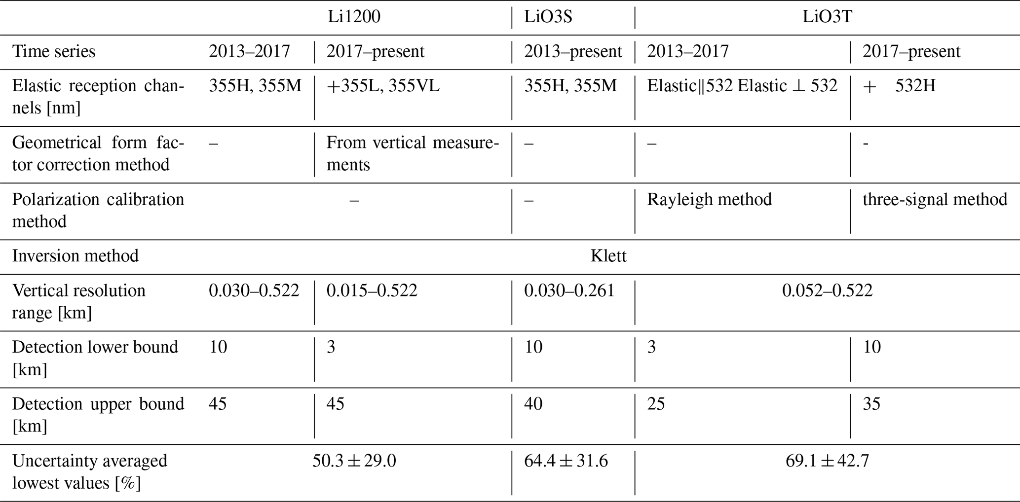
Table 1 is a summary of the characteristics of the three Maïdo lidars used to retrieve aerosol optical properties. A full description of each system is available in the following subsections.

Table 1 Systems technical features. The letters VL, L, M, and H after the wavelength stand for very low, low, medium, and high, respectively. Only aerosol channels are listed here.

2.1 Lidar 1200 (Li1200)

Lidar 1200 (Li1200) is a Rayleigh–Raman lidar able to measure vertical profiles of temperature between 30 and 100 km a.s.l. and water vapor ratio from the ground up to 18 km (Vérèmes et al., 2019). Vertical profiles of aerosol light extinction and backscattering can also be retrieved from the raw signals as this instrument provides Rayleigh–Mie scattering at 355 nm and Raman N₂ scattering at 387 nm. This instrument has been operating at the Maïdo facility since 2012 and has produced data since 2013.

2.1.1 Actual configuration

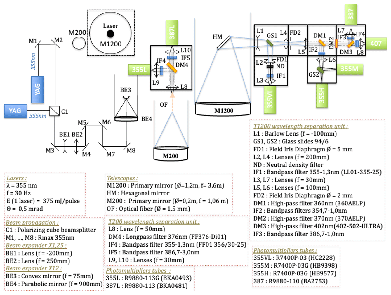
• The emission. It consists of two Pro-290 Nd:YAG lasers of the Quanta-Ray Pro series from Spectra-Physics emitting electromagnetic pulses at 1064 nm and 30 Hz (https://www.laserlabsource.com/files/pdfs/solidstatelasersource_com/product-305/Nd_Yag_Laser_Nanosecond_Laser_1064nm_1250mJ_Spectra_Physics-1462086952.pdf, last access: 10 July 2024). The final wavelength emitted is 355 nm, which corresponds to the third harmonic of the initial wavelength. Each pulse delivers 375 mJ in 9 ns. The optical design of this lidar is represented in Fig. 1. The two laser beams are recombined through a polarizer cube and then sent to the telescope through a series of mirrors. It should be noted that the lasers and the telescope are not in the same room, hence the use of many mirrors. BE1 and BE2 lenses form an afocal lens of a magnification of 1.25, reducing the divergence of the beams and mixing the phases. The goal is to reduce the hot spots, especially on the very fragile optic BE3 lens. Lastly, the laser beam is channeled through the center of the main telescope and magnified by a factor of 10 thanks to the afocal systems BE3 and BE4. The emission and main reception are therefore static coaxial, reducing the parallax effect and the minimum overlap altitude.

• The reception. It is made of two telescopes. The main telescope consists of a primary mirror of 1200 mm diameter (M1200), which gave its name to this instrument. A secondary mirror, HM, sends the beam to the detection system. The L1 lens allows the beam to converge faster, which explains the 3.6 m value of the focal length. GS1 is a glass plate that sends about 8 % of the beam to the 355 nm very low (355VL channel) detector. As this detector is located before the FD2 diaphragm, its field of view is the same as the one of the telescope, and it receives a signal at very close range. A density filter (ND) was placed in front of this detector to avoid saturation. FD2 is a diaphragm located at the focal plane of the telescope. Its aperture improves the geometrical factor of the telescope for the detectors following it. DM1 is a dichroic filter that reflects 355 nm and allows 387 and 407 nm to pass through. GS2 is a glass plate that sends about 8 % of the beam through the 355 nm medium (355M) channel and 92 % of the beam through the 355 nm high (355H) channel. DM3 is a dichroic filter which selects the 387 nm for the Raman N₂ channel. As of 2017, a second telescope, with a 200 mm M200 primary mirror and a focal length of 1 m, sends the signal to a second detection box using an optical fiber. This detection box filters the Rayleigh and Raman signals and channels them, respectively, to the 355L and 387L detectors.

• The detectors. All of them are photomultiplier tubes (PMTs) from Hamamatsu, reconditioned by the Licel company (https://www.hamamatsu.com/content/dam/hamamatsu-photonics/sites/documents/99_SALES_LIBRARY/etd/PMT_TPMZ0002E.pdf, last access: 10 July 2024). The 355H, 355M, and 355L detectors are electronically shuttered to prevent saturation. The acquisition cards are also by Licel and operate in photo-counting mode. There are no analog channels. Raw files follow a 1 min integration period.

• The summary. To summarize, 355M and 355H channels have existed since 2013, but their acquisition starts at 15 and 25 km, respectively, to avoid saturation. Hence, the 355VL and 355L channels were added in 2017 to cover the first altitude ranges, comprising the ground level up to an altitude of 15 km. The minimum height for 355L electronic shuttering is 450 m a.s.l.

2.1.2 Previous modifications

The detection unit was modified in 2017. Before that, the detection unit containing the 355L and 387VL detectors did not exist. The M1200 mirror separation unit was modified. First, the part that connecting the FD1 to L3 optics as well as the 355VL detector did not exist. There was an optic between IF2 and DM2 that would send the visible signal to another detection unit. Indeed, originally, this lidar was supposed to operate at two emission wavelengths, 355 and 532 nm. However, during installation, due to mechanical and optical problems, only the 355 nm channel was retained (Dionisi et al., 2015).

Figure 1 Li1200 optical scheme.

2.2 Stratospheric ozone lidar (LiO3S)

The stratospheric ozone lidar (LiO3S) works with the DIfferential Absorption Lidar (DIAL) technique and provides vertical profiles of ozone (O₃) concentration in the stratosphere between the tropopause and about 45 km (Godin-Beekmann et al., 2003; Portafaix et al., 2003). To this end, two different wavelengths are emitted: a 308 nm signal strongly absorbed by ozone molecules and a 355 nm signal weakly absorbed by ozone molecules. Vertical profiles of aerosol light extinction and backscattering can be retrieved from the elastic scattering at 355 nm and Raman N₂ scattering at 387 nm. From 2000 to 2012, LiO3S was located at the Moufia University campus in Saint-Denis and provided ozone vertical profiles. It was moved to the Maïdo facility in 2012 and has been measuring from this location since 2013.

2.2.1 Actual configuration

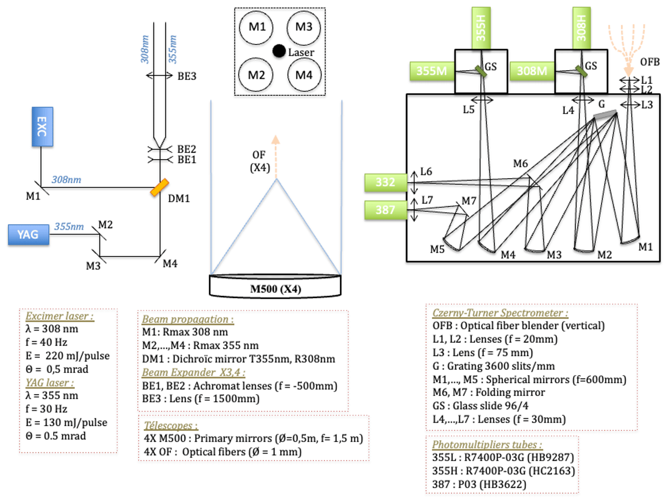
• The emission setup. It consists of two different lasers. An IPEX-840 PulseMaster PM-800 series excimer laser with XeCl gas from LightMachinery (https://lightmachinery.com/lasers/excimer-lasers/ipex-800/, last access: 10 July 2024) emits electromagnetic pulses at 308 nm with a frequency of 40 Hz and pulse energy of 220 mJ. A Lab-150 Nd:YAG laser of the Quanta-Ray Lab series from Spectra-Physics emits an electromagnetic pulse at 1064 nm, with a frequency of 30 Hz (https://www.laserlabsource.com/files/pdfs/solidstatelasersource_com/product-305/Nd_Yag_Laser_Nanosecond_Laser_1064nm_1250mJ_Spectra_Physics-1462086952.pdf, last access: 10 July 2024). The final wavelength emitted by the Nd:YAG laser is 355 nm, which corresponds to the third harmonic of the emitted wavelength. The pulse energy at this wavelength is 130 mJ. The laser beam diameter is about 10 mm, and its divergence is 0.5 mrad. The optical design of this lidar is shown in Fig. 2. Again, the emission and reception of this lidar are located in different rooms, explaining the use of many mirrors. The expander consists of three lenses, BE1, BE2, and BE3, magnifying the signal by a factor 10. The final beam has a 100 mm diameter.

• The reception. It is made of four 500 mm diameter telescopes. The primary mirrors are M1, M2, M3, and M4. The signal is emitted at the center of these telescopes, and the distance between the emission and the center of each telescope is 600 mm. At the receiving end, the signal is focused from each telescope to a corresponding optical fiber, all of which are positioned in a line before the signal enters the detection box. In this box, a diffraction grating separates the different wavelengths. Internal mirrors allow the beam to be reflected in the detectors. Finally, a glass plate discriminates the high- and low-energy channels at 355 nm.

• The detectors. These are all photomultiplier tubes (PMTs) from Hamamatsu, reconditioned by the Licel company (https://www.hamamatsu.com/content/dam/hamamatsu-photonics/sites/documents/99_SALES_LIBRARY/etd/PMT_TPMZ0002E.pdf, last access: 10 July 2024), and the signal acquisition cards are from Licel. The 355 nm detectors are electronically shuttered to avoid saturation. The acquisition is in photo-counting mode only for the high-energy channels, and in photo-counting and analog mode for the low-energy channels. Raw files follow a 1 min integration.

2.2.2 Previous modifications

Before 2017, the electronic obturation concerned only 355H and 308H channels, and a mechanical chopper shuttered 355M, 308M, and Raman channels at the entrance of the detection box. In 2017, this chopper malfunctioned and was replaced by electronic obturation for the 355M and 308M channel. Raman channels were not shuttered anymore. The initial integration time was 3 min and was reduced to 2 and then 1 min. During this period, the vertical resolution was modified from 120 to 15 m.

Figure 2 LiO3S optical scheme.

2.3 Tropospheric ozone lidar (LiO3T)

The tropospheric ozone lidar (LiO3T) also works with the DIAL technique and provides vertical profiles of ozone (O₃) concentration in the troposphere between 6 and 25 km (Duflot et al., 2017). To this end, two different wavelengths are emitted using stimulated Raman scattering: a 289 nm signal strongly absorbed by ozone molecules and a 316 nm signal weakly absorbed by ozone molecules. Vertical profiles of aerosol light extinction and backscattering can be retrieved from the residual emission of the laser in terms of elastic scattering at 532 and 1064 nm and Raman N₂ scattering at 607 nm. From 1993 to 2012, LiO3T was located at the Moufia University campus in Saint-Denis and provided ozone vertical profiles. It was moved to the Maïdo facility in 2012 and has been measuring from this location since 2013. The first aerosol-dedicated polarized channels were installed in 2014.

2.3.1 Actual configuration

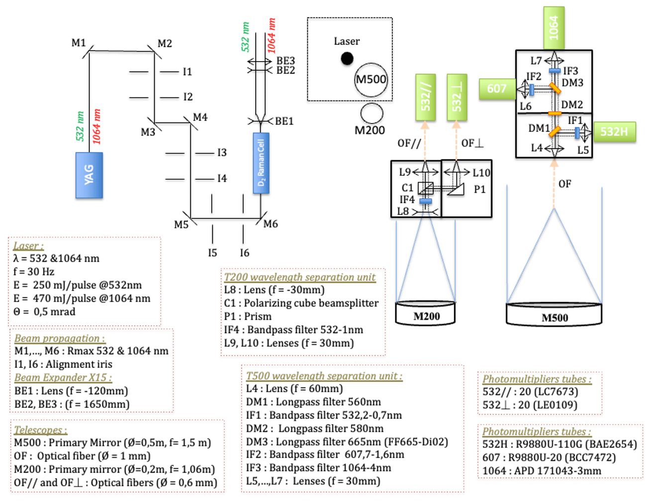
• The emission. It consists of a Pro-290 Nd:YAG laser of the Quanta-Ray Pro series from Spectra-Physics initially emitting at 1064 nm at 30 Hz (https://www.laserlabsource.com/files/pdfs/solidstatelasersource_com/product-305/Nd_Yag_Laser_Nanosecond_Laser_1064nm_1250mJ_Spectra_Physics-1462086952.pdf, last access: 10 July 2024). While the fourth harmonic (266 nm) is used to retrieve tropospheric ozone profiles (by its passage through a Raman cell generating 289 and 316 nm pulses), we use the second harmonic (532 nm) to retrieve aerosol light extinction and backscattering. Each pulse at 532 nm provides energy of 250 mJ. The laser beam diameter is about 10 mm, and its divergence is about 0.5 mrad. The optical design of this lidar for aerosol measurements is represented in Fig. 3. Again, the emission and reception of this lidar are located in different rooms, explaining the use of many mirrors. The lenses, BE1, BE2, and BE3, magnify the signal by a factor of 15. The final emitted beam has a diameter of 100 mm.

• The reception. It consists of two telescopes: one for the Rayleigh and Raman channels (532, 607, and 1064 nm, respectively) and the other for the polarized channels, at 532 nm. The first telescope (M500) consists of a 500 mm diameter primary mirror. An optical fiber located at its focal point conducts the signal to the detection box. Dichroic filters separate the 532, 607, and 1064 nm wavelengths. The second telescope consists of a 200 mm diameter primary mirror immediately followed by a polarizing cube. An optical fiber leads the polarized and cross-polarized beams to the interference filters and to the detectors.

• The detectors. They are all photomultiplier tubes (PMTs) from Hamamatsu, reconditioned by the Licel company (https://www.hamamatsu.com/content/dam/hamamatsu-photonics/sites/documents/99_SALES_LIBRARY/etd/PMT_TPMZ0002E.pdf, last access: 10 July 2024) except for the 1064 nm detector, which is an avalanche diode with a 3 mm diameter sensor (https://www.hamamatsu.com/content/dam/hamamatsu-photonics/sites/documents/99_SALES_LIBRARY/ssd/si_apd_kapd0001e.pdf, last access: 10 July 2024). The 532 high-energy channel (532H) detector is the only one electronically shuttered. All the acquisition cards are from Licel. The acquisition of the 532 nm polarized channel as well as the 607 nm channel is in photo-counting mode. The acquisition of the 532H channel is in photo-counting and analog modes, and the acquisition of the 1064 nm channel is only in analog mode. Raw files follow a 2 min integration period.

2.3.2 Previous modifications

In 2014, the 200 mm telescope (M200) and the T200 wavelength separation unit were installed, allowing for the first aerosol measurements with polarized channels. In 2017, one of the four 500 mm telescopes initially dedicated to ozone measurements was used for aerosol measurements. A second detection box was added, enabling the 607 and 1064 nm channels acquisition.

Figure 3 LiO3T optical scheme.

3 Routine measurements

The Maïdo lidars are research instruments that require manual handling and a constant human presence while operating. Maïdo observatory is a high-altitude facility (2160 m a.s.l.) and is located above the boundary layer in the free troposphere during the night. Acquisitions are only made during the night to increase the signal-to-noise ratio (SNR). These instruments were originally intended for data observation in the stratosphere and the upper troposphere, so they are optimized to work at night and improve the SNR up to very high in the atmosphere. That is why acquisitions are only made during the night. Measurements also require the absence of low clouds or rain. The position of the Maïdo observatory on the west side of Réunion Island often protects the site from the clouds brought by trade winds. Notably, a ceilometer was installed at the Maïdo facility in 2019, and continuous observations revealed an average cloud frequency of, respectively, 20 % and 40 % during winter and summer nights (not shown).

Routinely, Maïdo lidars are operated two nights per week and measurements last from 7 pm to 1 am (local time, i.e., from 15:00 to 21:00 UTC). Specific campaigns (once or twice a year) can occasionally require significantly increasing the number of measurements. Operating these instruments implies following a strict, well-prepared protocol, including basic check-ups and laser power control. A metadata file is routinely fed with technical specifics for each night of observation and after any instrument modification. Automatization is currently in progress and could increase the frequency of routine measurements.

Maïdo lidars are large and cannot be moved to make horizontal measurements: the beams of the different lidars are always vertical. To avoid any problems with flying objects, a no-fly zone around the observatory is requested before each lidar measurement and during operating hours (exclusively nighttime). Access to the research building hosting these instruments is restricted. It is located far from any residential areas. The instruments themselves can only be accessed by trained authorized personnel equipped with personal protective equipment (including eye protection glasses for the laser wavelengths) and optical enclosures.

4 Data processing chain

4.1 Data processing levels

Our datasets follow a classification detailed in the following description. Data processing levels range from Level 0 to Level 2.

• i.

  Level 0 products (L₀) are uncorrected and uncalibrated raw data files in Licel format at full resolution produced by the instrument.

• ii.

  Level 1 products (L₁) provide cloud-free data cleaned from any instrument artifact (electronic parasites, synchronization problems, and power disruption, etc.). The cloud mask is currently manual. These corrections are essential for any user to be able to apply their own specific aerosol preprocessing without errors linked to the instrument itself or the weather.

• iii.

  Level 2 products (L₂) provide processed lidar data, including saturation correction, sky background correction, geometrical form factor correction, and gluing between high- and low-energy channels. These products also provide the aerosol optical properties and their corresponding uncertainties.

4.2 L₀-to-L₁ processing chain

Each instrument is equipped with an acquisition system provided by the Licel firm. The description of the acquisition program producing output files in Licel format can be downloaded at https://licel.com/raw_data_format.html (last access: 10 July 2024). This process concerns three main sources of interferences: (i) detection-related interferences, (ii) acquisition problems, and (iii) interferences linked to the lidar environment.

Any significant steps of this process are tagged in the L_1a output files to identify the corrections applied.

4.2.1 Detection interferences

Detection-related interferences can generally be linked to electromagnetic disturbances, which can occur in three different ways.

• i.

  An enhanced background signal concerning variable altitude ranges can impact the complete profile as shown in Fig. 4a. This disturbance affects one or several channels across a significant altitude range, making the data acquisition unusable and requiring its withdrawal. The strong disturbance in the signal made it easy to fully automatize their detection. Notably, obturated detectors are more sensitive to these disruptions. Experience has proven that they are directly related to the use of cell phones and walkie-talkies. These instruments have been banned from the instrument rooms during the measurements, significantly decreasing the frequency of these cases.

• ii.

  A second electronic problem that is often encountered comes from electronic gating. In fact, if a high-energy and a low-energy channel coexist, a peak can be observed in the low-energy channel raw signal at the gated altitude of the high-energy channel (Fig. 4b). This parasite peak usually appears in two consecutive range bins. This type of problem occurs when the detectors are obturated, and it can have a significant impact on the measurement. It is therefore necessary to remove the corresponding values and replace them by an averaged value between the previous and the following range bins.

• iii.

  The third detection disturbance corresponds to a sudden peak in the signal in a single randomly located range bin. This only concerns LiO3S and LiO3T. The consequence on the nighttime averaged profile is shown in Fig. 4c. Generally, the intensity of these spurious peaks is consistent and significantly higher than the atmospheric background noise. They are easily identified when the intensity of the received signal is much lower and become negligible with a stronger signal. However, there is an intermediate zone where the intensity of the received signal is close to the intensity of these peaks, making their detection more challenging. They are replaced by an averaged value.

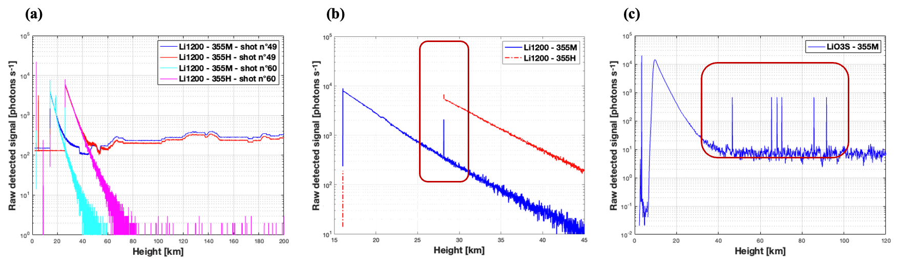
Figure 4 (a) Raw Li1200 signal – background signal anomaly, (b) raw Li1200 signal – peak from electronic gating, and (c) raw LiO3S nighttime averaged signal – random peaks in the far-range.

4.2.2 Acquisition problems

The acquisition program computes 1 or 2 min integrated profiles depending on the instrument. However, with this acquisition program, the measurement cannot be stopped at the end of the current cycle. As a result, the last file is generally shorter than the others and must be removed to guarantee consistent measurements.

Another issue was a time desynchronization of several minutes between the computer acquisition clocks in 2021, revealing a configuration fault in the corresponding Network Time Protocol time servers. Time differences could increase to up to 15 min between the different computers. This fault has been fixed and a time correction is applied for signals between 2012 and 2021.

Lastly, interaction between the different lidars working at the same time and emitting the same wavelength can also lead to interferences and disturbances in sensitive channels. To avoid this issue, the lasers are synchronized out of phase. However, errors with this offset can lead to files with a higher sky background than others. These files are removed.

4.2.3 Disturbance from clouds

The SNR is the most sensitive to the presence of low-altitude clouds. These clouds strongly absorb the emitted photons and lead to high extinction levels and weak SNRs. They must be removed. High-altitude cirrus clouds can also be removed if stratospheric aerosols are studied. Cloud detection can be automatic, manual, or both. An automatic detection of low clouds under 5 km in height has been developed and can be used from 2019 up to now using data from a Campbell CS135 ceilometer that was set up at the Maïdo facility in 2019. Manual cloud screening is done for any remaining cirrus or low clouds. Automatization is in progress for this time-consuming task.

4.3 L₁-to-L₂ processing chain

The goal of this second processing chain is to retrieve vertical profiles of aerosol optical products. It involves several key steps.

4.3.1 Saturation correction

Saturation affects photomultiplier tube detectors with an acquisition card in photo-counting mode. It concerns the lower layers of the atmosphere and appears when the number of backscattered photons overcomes the capacity of the acquisition card to discriminate them individually. Therefore, the backscattered signal is attenuated in the corresponding layers. On the contrary, acquisition in analog mode is not affected by saturation but has a weaker SNR.

One solution is to combine (namely glue together) analog and photo-counting channels if both are available, which is not always the case for our instruments.

The second option is to compare high- and low-energy channels (or analog and photo-counting channels if available) in the lower layers and apply a dead-time correction to the photo-counting channel using the Müller equation. This is the solution we adopted for Maïdo lidars concerning aerosol, which is similar to what is done for ozone and temperature processing (Leblanc et al., 2016a, b). The dead-time parameter (τ_d) corresponds to the minimum time for distinguishing between two consecutive photons. Our photo-counting modes are non-extensive, which means that the dead-time value is independent from the number of backscattered photons. We then apply the Müller equation (Müller, 1973):

$$\begin{array}{}\text{(1)}& S_{\mathrm{desat}}={\displaystyle \frac{S_{\mathrm{sat}}}{\mathrm{1}-{\mathit{\tau }}_{\mathrm{d}}\cdot \frac{c}{\mathrm{2}\cdot {\mathit{\delta }}_z\cdot L}\cdot S_{\mathrm{sat}}}},\end{array}$$

with S_sat (S_desat) corresponding to the saturated (desaturated) detected signal in photons per second, δ_z the vertical resolution in meters, c the light celerity in meters per second, and L the number of shots.

A value of τ_d=37 ns is chosen. This value is the one recommended by the Licel manufacturer and was confirmed after several experimental tests, the description of which is available in a summary document.

4.3.2 Background correction

The sky background signal (S_BC) is one of the main sources of noise affecting the SNR. It corresponds to (i) the detector noise and (ii) the natural light emitted by the atmosphere and can be affected by the presence of the moon during the night. The value of this signal is supposed to be constant with the altitude, but, in practice, it sometimes follows a linear variation due to the effect of the signal-induced noise on the detector. Our instruments are not equipped with a pre-trigger. Our method to calculate the S_BC value consists of performing a linear regression or an averaging of the desaturated signal in an altitude range high enough to neglect the impact of the backscattered signal compared to the S_BC, typically between 80 and 120 km.

4.3.3 Geometrical form factor correction

The overlap function, F(z), or crossover function, is one of the major sources of uncertainties for ground-based lidar measurements. It describes the fraction of the laser beam cross section contained by the telescope field of view as a function of range. Its values vary between 0 (blind zone, with no overlap) and 1 (full overlap). Originally, Maïdo lidars were designed to study the high troposphere and the stratosphere, and at these altitudes, the full overlap is obtained, which is why there has not yet been a more specific study on these instruments.

Should this parameter not be corrected, the received lidar signal would be attenuated between the blind zone and the full overlap, leading to incorrect optical values. Two approaches can be followed to determine this parameter. (i) A theoretical calculation using equations found in Measures (1984) can be performed. However, it implies having knowledge on several optical parameters which can vary over the time series, and different equations must be used for coaxial and biaxial systems. (ii) The second and most common approach is experimental and implies the use of horizontal measurements (Chazette et al., 2017). In fact, considering a constant and homogenous atmosphere along the line of sight, a linear regression can be performed in an altitude range high enough to be far from the full overlap. The difference between the logarithm of the signal and this linear regression gives an accurate estimation of F(z).

$$\begin{array}{}\text{(2)}& F\left(z\right)=\exp \left(\ln \right(S_{\mathrm{2}}\left(z\right))-y(z\left)\right),\end{array}$$

with S₂ being the desaturated, background-corrected, and range-corrected lidar signal; y(z) the linear regression; and z the altitude range.

It is physically impossible for these research instruments to measure horizontally. Therefore, the experimental approach using vertical measurements (instead of horizontal) in aerosol-free conditions was performed to correct overlap for the very low and low channels of lidar 1200. As of today, no overlap correction was needed for LiO3S (full overlap under 10 km) and LiO3T (full overlap between 3 and 4 km).

Figures 5a and 6a reveal the variability in the overlap function over the time series for both Li1200 VL and L channels. This variability can be explained by slight misalignments of the lidar. Indeed, given the important number of optical elements between the laser and the emission point, the risk of misalignment, even if minor, is significant. Figures 5b and 6b show the mean and standard deviation (SD) of the overlap function from an exponential regression. The small values of SD are an indicator of a low-varying function, a result that allows for the use of a unique overlap function rather than different functions for different periods. The estimated altitude of full overlap was 10 km for the very low channel and 15 km for the low channel.

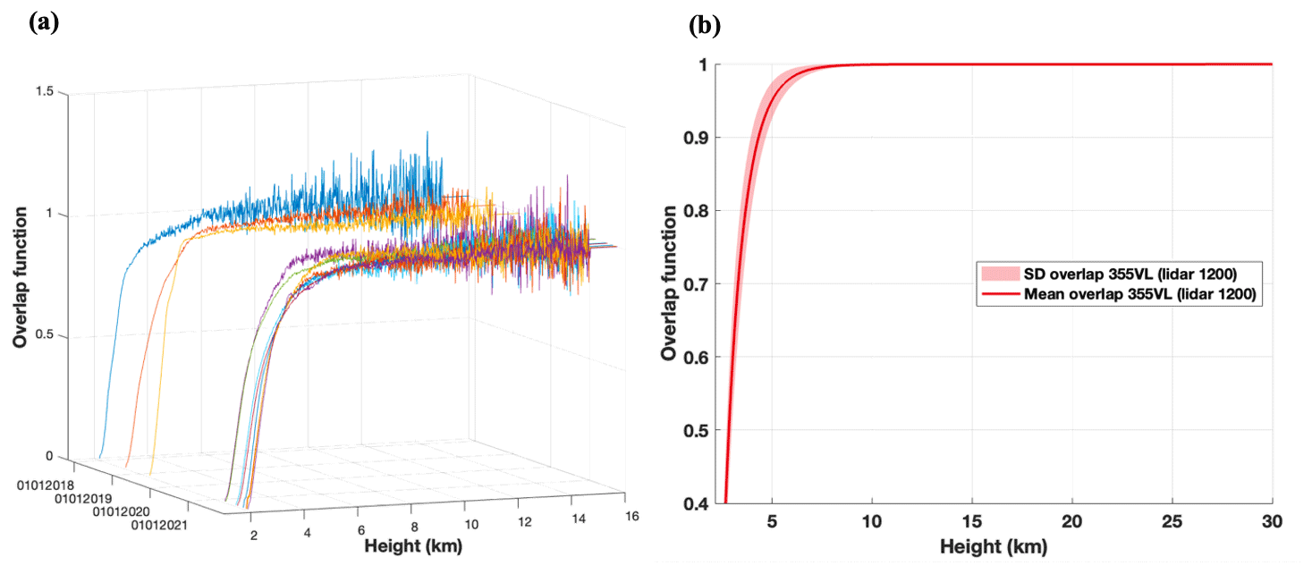
Figure 5 Li1200 VL channel. (a) Time series of overlap functions and (b) mean and standard deviation of the overlap function.

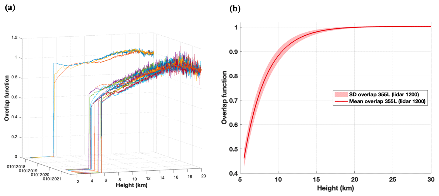
Figure 6 Li1200 L channel. (a) Time series of measured overlap functions and (b) mean and standard deviation of the exponential regression of the overlap function.

4.3.4 Smoothing

Smoothing is applied on the lidar signal to increase the accuracy of the retrieved aerosol profiles. For the three time series, smoothing was achieved using a low-pass filter with a Blackman window (Blackman and Tukey, 1958). The number of points for the filter was altitude-dependent and channel-dependent.

$$\begin{array}{}\text{(3)}& {\displaystyle }{S}_{\mathrm{filt}}\left(z\right)=S_{\mathrm{2}}\left(z\right)/F\left(z\right)\times {\displaystyle \frac{\mathrm{coef}}{\sum \mathrm{coef}}},\text{(4)}& {\displaystyle }\begin{array}{rl}\mathrm{coef}\left(n\right)& =\mathrm{0.42}-\mathrm{0.5}\times \cos \left({\displaystyle \frac{\mathrm{2}\mathit{\pi }n}{W-\mathrm{1}}}\right)+\mathrm{0.08}\\ & \times \cos \left({\displaystyle \frac{\mathrm{4}\mathit{\pi }n}{W-\mathrm{1}}}\right),\mathrm{0}\le n\le M-\mathrm{1},\end{array}\end{array}$$

with S_filt being the smoothed signal; S₂ the desaturated, background-corrected; and range-corrected lidar signal; M half the length of the window; and W the weight of the filter.

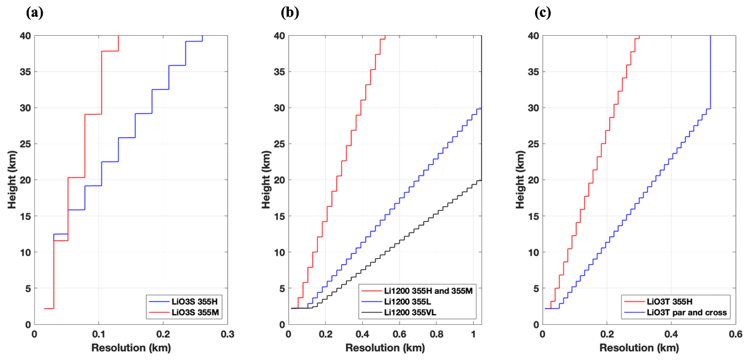
Figure 7a–c represent the new vertical resolution for each channel of each instrument. Two methods can be used to estimate vertical resolution after smoothing: (i) impulse response method and (ii) digital filter. The latter was chosen for these time series. It involves the mathematical calculation of the filter transfer function using a cutoff frequency of −3 dB (NDACC_resolDF; Leblanc et al., 2016a, b).

Figure 7 NDACC vertical resolution of (a) LiO3S, (b) Li1200, and (c) LiO3T.

4.3.5 Gluing together near- and far-range channels

High- and low-energy channels were combined for LiO3S and Li1200 using the gluing method of the square sinus and cosinus functions. The altitude range chosen for the gluing corresponded to a region where the high-energy channel was not affected by electronic distortions and the low-energy channel was not affected by too much noise.

$$\begin{array}{}\text{(5)}& {\displaystyle }\left\{\begin{array}{ll}\mathit{v}\mathbf{1}\left(z\right)=\mathrm{0},& z<\mathrm{altmin},\\ \mathit{v}\mathbf{1}\left(z\right)={\sin }^{\mathrm{2}}\left(\frac{\mathrm{0}\stackrel{n}{⟶}\mathrm{1}}{n}\times \frac{\mathit{\pi }}{\mathrm{2}}\right),& \mathrm{altmin}\le z\le \mathrm{altmax},\end{array}\right.\text{(6)}& {\displaystyle }\left\{\begin{array}{ll}\mathit{v}\mathbf{2}\left(z\right)=\mathrm{1},& z<\mathrm{altmin},\\ \mathit{v}\mathbf{2}\left(z\right)={\cos }^{\mathrm{2}}\left(\frac{\mathrm{0}\stackrel{n}{⟶}\mathrm{1}}{n}\times \frac{\mathit{\pi }}{\mathrm{2}}\right),& \mathrm{altmin}\le z\le \mathrm{altmax},\end{array}\right.\end{array}$$

with n being the number of range bins between altmin and altmax, v1 the vector to apply to the high-energy channel, and v2 the vector to apply to the low-energy channel.

The channels glued and used for inversion were (i) 355VL–355L–355M–355H and 355L–355M–355H and 355M–355H for Li1200 and (ii) 355H–355M for LiO3S. Each of these glued channels is available in the L_1b files. Inversion was applied for each glued channels, and the corresponding optical products can be found in the L₂ files.

4.3.6 Calibration depolarization value for LiO3T

Polarization channels enable the detection of changes in the backscattered polarization state produced by the atmospheric particles. The laser provides quasi-pure linear polarization. A polarizing cube beam splitter transmits the received linear polarized light and reflects the received cross-polarized light. It is necessary to determine the polarization calibration factor before combining the two signals (Biele et al., 2000).

Three methods can be used: (i) the Rayleigh calibration method (Behrendt and Nakamura, 2002), (ii) the ±45° or Δ90° calibration methods (Freudenthaler, 2016), and (iii) the three-signal (total, cross, and parallel) method (Reichardt et al., 2003). While the second and third method provide the smallest uncertainties, the first method can be used retrospectively if no total channel existed. The apparent volume linear depolarization ratio (VLDR^*) can then be calculated as follows:

$$\begin{array}{}\text{(7)}& {\mathrm{VLDR}}^{*}={\displaystyle \frac{K}{{\mathit{\eta }}^{*}}}\times {\displaystyle \frac{S_{\mathrm{r}}}{S_{\mathrm{t}}}},\end{array}$$

with t and r being the respective transmitted and reflected parts of the signal S, η^* the apparent calibration factor, and K the calibration factor correction parameter.

The VLDR can then be computed using the polarization crosstalk parameters for the transmitted and reflected signals (G_t,r and H_t,r) as follows:

$$\begin{array}{}\text{(8)}& \mathrm{VLDR}={\displaystyle \frac{{\mathrm{VLDR}}^{*}\left(G_{\mathrm{t}}+H_{\mathrm{t}}\right)-(G_{\mathrm{r}}+H_{\mathrm{r}})}{\left(G_{\mathrm{r}}-H_{\mathrm{r}}\right)-{\mathrm{VLDR}}^{*}\left(G_{\mathrm{t}}-H_{\mathrm{t}}\right)}}.\end{array}$$

The total signal will also be reconstructed as follows:

$$\begin{array}{}\text{(9)}& S_{\mathrm{total}}={\displaystyle \frac{\frac{{\mathit{\eta }}^{*}}{K}{H}_{\mathrm{r}}{S}_{\mathrm{t}}-H_{\mathrm{t}}{S}_{\mathrm{r}}}{H_{\mathrm{r}}{G}_{\mathrm{t}}-H_{\mathrm{t}}{G}_{\mathrm{r}}}}.\end{array}$$

The aerosol backscatter, β_a, is then deduced from the total signal, S_total, using Klett inversion. The backscatter ratio R is calculated as follows:

$$\begin{array}{}\text{(10)}& R={\displaystyle \frac{({\mathit{\beta }}_{\mathrm{a}}+{\mathit{\beta }}_{\mathrm{mol}})}{{\mathit{\beta }}_{\mathrm{mol}}}}.\end{array}$$

Finally, the particle linear depolarization ratio (PLDR) can be computed as follows:

$$\begin{array}{}\text{(11)}& \mathrm{PLDR}={\displaystyle \frac{\left(\mathrm{1}+{\mathrm{LDR}}_{\mathrm{mol}}\right)\times \mathrm{VLDR}\times R-\left(\mathrm{1}+\mathrm{VLDR}\right)\times {\mathrm{LDR}}_{\mathrm{mol}}}{\left(\mathrm{1}+{\mathrm{LDR}}_{\mathrm{mol}}\right)\times R-\left(\mathrm{1}+\mathrm{VLDR}\right)}}.\end{array}$$

In our case, we used the Rayleigh method before 2017 and the three-signal method after 2017. We used a linear molecular depolarization ratio (LDR_mol) of 0.00398 at 532 nm (Behrendt and Nakamura, 2002) to estimate η^* and a K factor of 1 to estimate VLDR^*. The following crosstalk parameter values were considered ideal: G_t=1, H_t=1, G_r=1, and $H_{\mathrm{r}}=-\mathrm{1}$.

4.3.7 Optical products – Klett inversion

This step is mandatory to retrieve aerosol optical properties from the detected lidar signals. However, it implies resolving a first-order Bernoulli equation with several unknown parameters. Several methods exist, such as (i) one- or two-component Klett inversion (Klett, 1981, 1985), (ii) Raman inversion (Ansmann et al., 1990, 1992), and (iii) synergistic method using Klett inversion and sun photometer measurements to evaluate the lidar ratio (Raut and Chazette, 2007).

Because Raman channels currently have a very low SNR, they are not included in this work, and the two-component Klett inversion method was chosen for the three systems. It implies the determination of an a priori constant value of the lidar ratio (LR) and a clean, aerosol-free zone in the atmosphere (Rayleigh zone). Details about the elastic two-component algorithm from Klett are available in Appendix A.

The solution proposed in Appendix A is

$$\begin{array}{}\text{(12)}& \begin{array}{rl}& \mathit{\beta }(\mathit{\lambda },z)={\mathit{\beta }}_{\mathrm{a}}(\mathit{\lambda },z)+{\mathit{\beta }}_{\mathrm{m}}(\mathit{\lambda },z)\\ & ={\displaystyle \frac{S_{\mathrm{2}}(\mathit{\lambda },z)\cdot \exp \left\{\mathrm{2}\cdot {\int }_{z^{\prime }=z}^{z_{\mathrm{ref}}}\left(\frac{{\mathrm{LR}}_{\mathrm{a}}(\mathit{\lambda },z^{\prime })}{{\mathrm{LR}}_{\mathrm{m}}(\mathit{\lambda },z^{\prime })}-\mathrm{1}\right)\cdot {\mathit{\alpha }}_{\mathrm{m}}(\mathit{\lambda },z^{\prime })\mathrm{d}{z}^{\prime }\right\}}{\begin{array}{c}\frac{S_{\mathrm{2}}(\mathit{\lambda },z_{\mathrm{ref}})}{\mathit{\beta }(\mathit{\lambda },z_{\mathrm{ref}})}+\mathrm{2}\cdot {\int }_{z^{\prime }=z}^{z_{\mathrm{ref}}}{\mathrm{LR}}_{\mathrm{a}}(\mathit{\lambda },z^{\prime })\cdot S_{\mathrm{2}}(\mathit{\lambda },z^{\prime })\\ \cdot \exp \left\{\mathrm{2}\cdot {\int }_{x^{\prime }=z}^{z_{\mathrm{ref}}}\left(\frac{{\mathrm{LR}}_{\mathrm{a}}(\mathit{\lambda },x^{\prime })}{{\mathrm{LR}}_{\mathrm{m}}(\mathit{\lambda },x^{\prime })}-\mathrm{1}\right)\cdot {\mathit{\alpha }}_{\mathrm{m}}(\mathit{\lambda },x^{\prime })\mathrm{d}{x}^{\prime }\right\}\cdot \mathrm{d}{z}^{\prime },\end{array}}}\end{array}\end{array}$$

with a (m) being the particular (molecular) contribution, α(λ,z) (β(λ,z)) the summed molecular and particular extinction (backscatter), and LR the lidar ratio. S₂ corresponds to the range-corrected, sky-background-corrected, and desaturated signal. However, the signal used in this study for the inversion algorithm is smoothed as explained in Sect. 4.3.4 and could be glued (Li1200 and LiO3S) or recombined (LiO3T).

Several unknown parameters must be determined as follows:

• i.

  To retrieve the LR_a, we chose a constant LR value of 50 sr for the three instruments to be consistent between the time series and to target the most frequent aerosol types. Moreover, it enables easier comparisons with satellite data such as Cloud-Aerosol Lidar with Orthogonal Polarization (CALIOP) products (Cattrall et al., 2005).

• ii.

  The equation used to retrieve the molecular extinction was (Bates, 1984)

  $$\begin{array}{}\text{(13)}& {\mathit{\alpha }}_{\mathrm{m}}(\mathit{\lambda },z)={\displaystyle \frac{P}{k\times T}}\times {\displaystyle \frac{\mathrm{4.02}\times {\mathrm{10}}^{-\mathrm{28}}}{{\mathit{\lambda }}^{\mathrm{4}+(\mathrm{0.389}\mathit{\lambda }+\mathrm{0.09426}{\mathit{\lambda }}^{-\mathrm{1}}-\mathrm{0.3228})}}},\end{array}$$

  with k corresponding to the Boltzmann constant. Atmospheric pressure, P, and temperature, T, were retrieved from the Arletty AERIS product (https://www.aeris-data.fr/, last access: 30 March 2024), relying on data from the European weather forecast model by ECMWF (European Centre for Medium-Range Weather Forecasts) and producing interpolated data every 6 h around Maïdo observatory (Hauchecorne, 1998).

  The molecular backscatter was then computed as follows:

  $$\begin{array}{}\text{(14)}& {\mathit{\beta }}_{\mathrm{m}}(\mathit{\lambda },z)={\mathit{\alpha }}_{\mathrm{m}}(\mathit{\lambda },z)\times {\displaystyle \frac{\mathrm{3}\times K_{\mathrm{f}}}{\mathrm{8}\mathit{\pi }}}.\end{array}$$

  The King factor value (K_f) is considered equal to 1 (King, 1923), and $\frac{\mathrm{3}}{\mathrm{8}\mathit{\pi }}$ corresponds to the LR_m.

  The last step was to determine a reference “Rayleigh” zone, z_ref, that is supposedly free of aerosols for each daily measurement and each channel.

4.3.8 Raman and 1064 nm channel issues

Klett inversion brings about the problem of considering a lidar ratio constant with height. In fact, a single aerosol plume is often made of several layers of particles with heterogenous backscattered lidar signals. Raman inversion is one solution to differentiating between a vertical profile of lidar ratio from elastic and Raman channels. However, our Raman channels have a poor SNR and are not usable for stratospheric or high tropospheric aerosols. The retrieval of aerosol optical products using Raman inversion for low-energy channels (low and middle troposphere) is still ongoing. There is also a misalignment issue for the 1064 nm channel, leading to a poor SNR. This channel is currently unexploitable.

5 Quality assessment

5.1 Database statistics

A total of 1737 nighttime measurements were preprocessed between 2013 and 2023: 710 files for Li1200, 534 files for LiO3S, and 493 files for LiO3T. Notably, the mean percentage of rejected files was higher for Li1200 (52.7 %) than for LiO3T (44.8 %) and LiO3S (32.7 %). Figure 8 shows the cumulated monthly number of validated L₂ profiles for each instrument, the monthly mean number of rejected files, and the corresponding tags (cloud detection, technical issue, low SNR). It should be noted that more observations were made during the period from May to November (austral winter, dry season) compared to the period from December to April (austral summer, wet season), which is consistent with the higher cloud and rain occurrence during the wet season. The mean percentage of validated L₁ files was 62.4 % during the dry season and 48.5 % during the wet season. The lower frequency of measurements in January, July, August, and December also coincides with two important holiday periods. The frequency of technical issues and lower SNR is statistically higher during the months with a greater number of measurements.

Figure 8 Number of validated files for the three instruments in the period 2013–2023. The table at the bottom shows the mean percentage of rejected files and tagged files for each month.

5.2 Instrument capabilities

The gluing technique allowed for the determination of different altitude ranges for each lidar depending on the channels available. Table 1 provides a summary of the theoretical instrument performances in terms of altitude ranges. Apart from the number of channels glued together, other parameters can influence the maximum altitude (SNR) or the minimum altitude (overlap, SNR) of the validated L₂ vertical profile. LiO3T at 532 nm is ideal for investigating the low and mid troposphere. The high troposphere and stratosphere can be studied at 355 nm (Li1200 and LiO3S) or 532 nm (LiO3T – from 2017 until now).

5.3 Instrument intercomparison

In this study, we performed a comparison between the three instruments to detect any major discrepancies using the stratospheric aerosol optical depth (sAOD) between 17 and 30 km. Figure 9 displays the time series of sAOD at 355 nm (Li1200 and Li03S) for concomitant measurements and corresponding uncertainties. There is a good overall consistency between the two instruments. The differences between the two time series could be the consequence of technical modifications (channel addition, optimization, and misalignment). Three peaks periods of high sAOD values can be identified: the emission of volcanic aerosols in the stratosphere during the Hunga Tonga eruption in 2022 (Kloss et al., 2022; Baron et al., 2023; Sicard et al., 2024), the Calbuco volcanic eruption in 2015 (Bègue et al., 2017), and the Australian bushfires in 2020 (Khaykin et al., 2020). Higher differences in 2021 could be the consequence of repeated misalignments for Li1200.

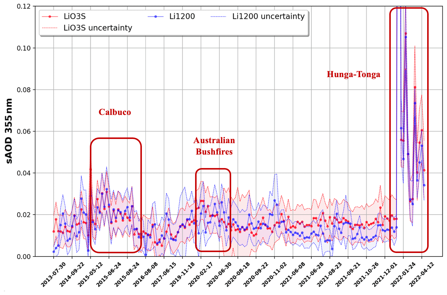
Figure 9 Nighttime AOD (17 to 30 km layer) at 355 nm from Li1200 (red) and LiO3S (blue) (concurrent measurements) with corresponding uncertainties (dashed colored lines). Exceptional events circled in red. The horizontal timeline is not linear: one date out of eight is represented for visual purposes.

The dispersion of sAOD values is represented in Fig. 10. The sAOD at 355 nm varies between 0.001 and 0.107 for LiO3S and Li1200, with a mean of 0.019 ± 0.012 and 0.017 ± 0.012, respectively. A good correlation is found between the two lidars (correlation R=0.924 ± 0.005).

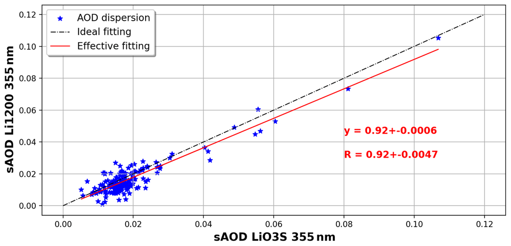
Figure 10 Dispersion of the AOD (17 to 30 km layer) at 355 nm between Li1200 and LiO3S. The red line represents the theoretical linear regression.

The correlation between the two instruments at 355 nm in terms of extinction values is higher above 17 km but lower from 10 to 17 km (Appendix D, Fig. D1). In fact, for Li1200, (i) low-energy channels were added in 2017; (ii) there were changes in the minimal altitude of detection for the 355M channel; and (iii) this instrument had many misalignments and underwent several optical upgrades, leading to modifications of the overlap function.

For further retrospective trend studies, it is important to note that LiO3S has been the most stable instrument throughout the time series and is considered the reference instrument at 355 nm. However, data from Li1200 can be used to fill the gaps not only in the LiO3S database depending on the altitude range targeted, but also for specific case studies with the need for the retrieval of optical products for the middle and low troposphere.

The same analysis was performed for LiO3T. To compare the two wavelengths, Ångström exponents (AEs) were computed between LiO3T (532 nm) and alternatingly LiO3S (355 nm) and Li1200 (355 nm). Figure 11 shows the dispersion of AE values. The order of magnitude of AE values varies between 0.0794 and 1.288, with a mean of 0.56 ± 0.29 and 0.54 ± 0.28, respectively. Again, a good correlation is found between both datasets (R=0.901 ± 0.128). These values also demonstrate the variability in stratospheric aerosol size distribution between 17 and 30 km (Gobbi et al., 2007; Burton et al., 2012).

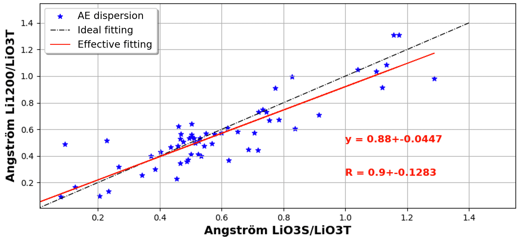
Figure 11 Dispersion of the AE (17 to 30 km layer) between 355 and 532 nm. The black line represents the theoretical linear regression and the red line the actual linear regression.

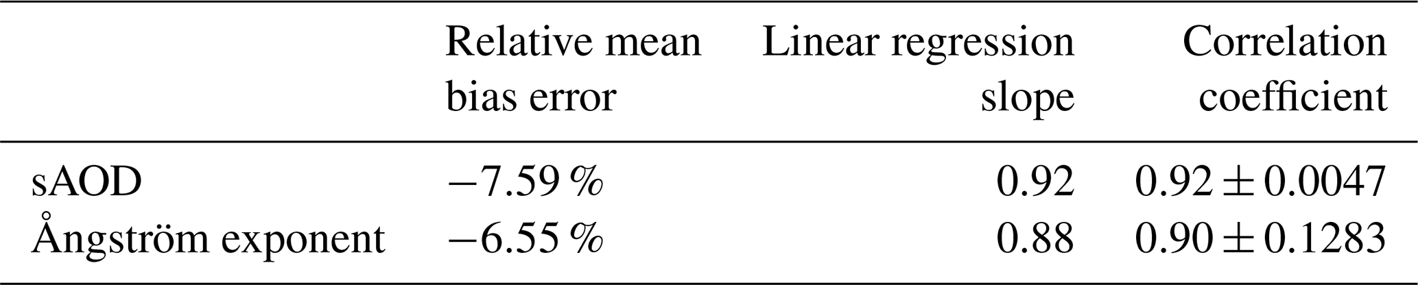
Table 2 summarizes the metrics used to intercompare the three instruments. The relative mean bias error (MBE) was added to the analysis. After identifying LiO3S as the reference instrument at 355 nm, we found a negative MBE (−6.55 %) concerning sAOD, meaning that Li1200 tends to underestimate sAOD compared to LiO3S.

Table 2 Intercomparison between the three instruments in terms of sAOD and Ångström exponent.

5.4 Main sources of uncertainties

The total uncertainty budget of each lidar is described in Appendix B. Four sources of uncertainty were propagated in quadrature (Sicard et al., 2009; Rocadenbosch et al., 2010): (i) uncertainty due to the Rayleigh calibration value (u_altref); (ii) uncertainty due to the lidar ratio value (u_LR), with a distinction between LR, top and LR, bottom defining the respective upper and lower error bars; (iii) uncertainty due to the SNR vertical distribution (u_SNR); (iv) and uncertainty due to the SNR value at the calibration altitude (u_{SNR, altref}). Figure 12a–c represent the importance of each uncertainty in relation to the total backscatter in percentage for three case reports, and Fig. 12d–f represent the corresponding propagated total backscatter uncertainty for the three instruments.

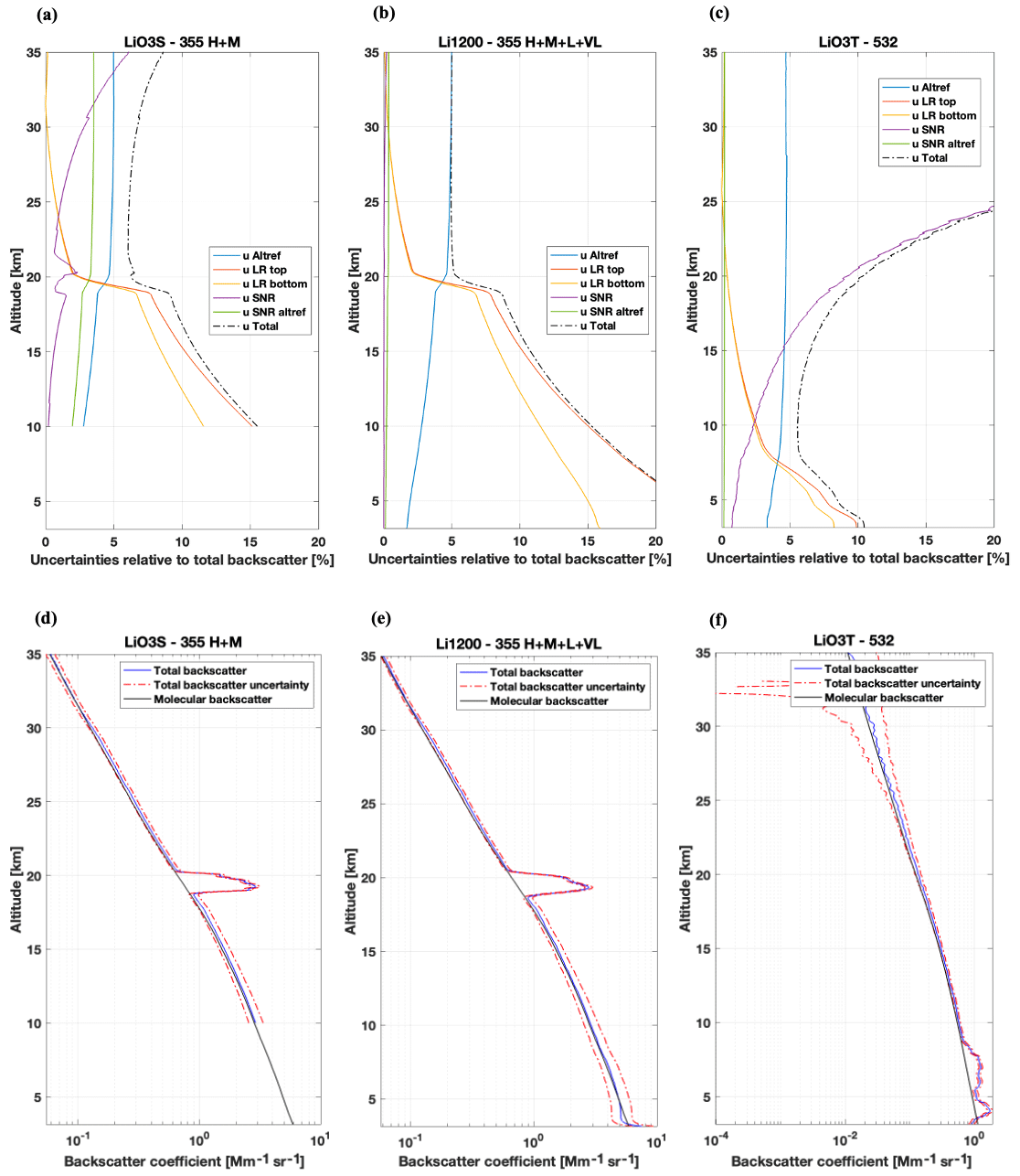
Figure 12 (a–c) Random cases showing the molecular backscatter (black) and the backscatter coefficient (blue) and its apparent uncertainty (red dotted line) for (a) LiO3S (25 January 2022), (b) Li1200 (25 January 2022), and (c) LiO3T (25 September 2017). (d–f) Corresponding relative uncertainties for (d) LiO3S, (e) Li1200, and (f) LiO3T.

In Fig. 12a–c, the behavior of uncertainties u_altref (blue curves) and u_{SNR, altref} (green curves) is stable over the different altitude ranges. Notably, u_altref comes from the 5 % uncertainty in the molecular backscatter, which determines the lower threshold for the total uncertainty. The u_SNR uncertainty (purple curves) is strongly influenced by the altitude, with minimal values at lower altitude ranges, where the lidar signal is stronger, and values increasing with the altitude. In fact, lidar signals are filtered before inversion, making u_SNR the predominant error at higher altitude levels. Oppositely, the u_LR uncertainty (orange and yellow curves) is the lowest at the calibration altitude and increases at the lower levels, where it becomes predominant. The systematic uncertainty in the LR value was set to 30 % for this study. Therefore, the total uncertainty is the lowest in mid-altitude ranges before it increases in lower and higher altitude levels. Sharp spikes in u_LR can be observed just below 20 km for LiO3S and Li1200 and below 8 km for LiO3T. They are linked to the presence of aerosol plumes and emphasize the impact of aerosols on the uncertainty values in lower altitude levels.

For LiO3S (H–M glued channel), the total relative uncertainty reaches 15 % at 10 km, decreases to 6 % around 20 km, and increases to up to 8 % around 35 km. (Fig. 12a). Without the aerosol layer, the minimum error would be reached around 15 km. For Li1200 (H–M–L–VL glued channel), the total relative uncertainty reaches 20 % at 7 km and decreases down to 5 % from 20 km up (Fig. 12b). The uncertainty due to the SNR is very low compared to LiO3S as this instrument is designed to reach very high-altitude levels, and the signal used for inversion is made of four filtered signals with complementary vertical capacities. Without the aerosol layer, the minimum error would be reached around 17 km. For LiO3T, the total relative uncertainty reaches 10 % at 4 km, decreases to 6 % around 8 km, and increases to up to 20 % around 25 km. (Fig. 12c). The uncertainty due to the SNR is higher than in the previous lidars because this instrument is designed for tropospheric measurements.

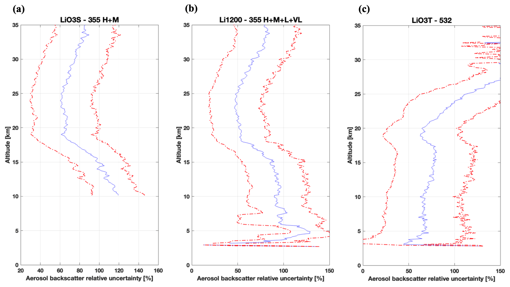
Figure 13 Mean (blue line) and standard deviation (dotted red line) of the time series of relative uncertainty from the inversion technique for (a) lidar O3S (H–M channel), (b) lidar 1200 (H–M–L–VL channel), and (c) lidar O3T (polarized channels).

In Fig. 12d–f, the three instruments demonstrate their capacity to detect aerosol layers with relatively low error rates and a high resolution. Figure 12d–e specifically show their ability to identify variations within the aerosol layer between 18 and 20 km. For LiO3T (Fig. 12f), the aerosol layer between 4 and 8 km is exceptionally well defined, with relatively low error values. Apart from these aerosol layers, the molecular backscatter (in black) tends to align closely with the uncertainty in the total backscatter (in red). In fact, background aerosols are characterized by very low backscatter and extinction values, leading to the relatively high sAOD uncertainties observed in Fig. 9, which is higher for background aerosols but lower for cases with a stronger aerosol load, such as from Australian fires or volcanic aerosols. Focusing on the uncertainty specific to aerosol backscatter (rather than the total) is essential to improve the uncertainty analysis along with a statistical analysis of the dataset to minimize disruptions caused by transient aerosol events. Time series of aerosol backscatter relative total uncertainties were computed for the three instruments, and the corresponding mean and standard deviation are represented in Fig. 13a–c. Values are high and easily reach 100 % for the three instruments because of the very low values of aerosol backscatter coefficients above Maïdo observatory. The mean uncertainty is the lowest for LiO3S between 18 and 25 km (64.4 ± 31.6 %). It increases under 18 km and above 25 km, with relative uncertainty values reaching more than 100 % due to the very weak aerosol backscatter values at these altitude ranges. The mean uncertainty for Li1200 is also the lowest between 18 and 25 km (50.3 ± 29.0 %). It increases under 18 and above 25 km, with relative uncertainty values that are relatively lower than LiO3S due to a lower SNR and the presence of low and very low channels detecting aerosol plumes at lower altitudes. LiO3T exhibits a low relative uncertainty below 20 km, which varies and is around 69.1 ± 42.7 %. The strong increase above 20 km is essentially explained by the very low SNR for this instrument at these altitude ranges.

Table 3 provides a summary of the processing method and the area of validity of the Level 2 products.

Table 3 Summary of the processing method and area of validity for the Level 2 products.

6 Data availability

Raw L₀ files, cleaned L₁ files, and processed L₂ files with optical products are generated locally. L₀ files are made of 1 min integrated raw files in Licel format. L₁ products contain 1 min integrated time series and overnight averaged cleaned signals in MAT file format and netCDF format. L₂ products in MAT file format contain overnight averaged processed signals as well as range-corrected signals for Raman channels. L₂ products are also computed in netCDF format following NDACC guidelines in anticipation of a future NDACC label request. Table C1 in Appendix C summarizes the optical products and other variables available in these L₂ netCDF files.

Each of these files is available upon request in our local data center via File Transfer Protocol (FTP; ftp://tramontane.univ-reunion.fr/, last access: 10 September 2024, Gantois et al., 2024). L₁ and L₂ files are currently available at https://doi.org/10.26171/rwcm-q370 (Gantois et al., 2024). MAT files and netCDF files with L₂ data will soon be available on the AERIS database, but only L₂ netCDF files will be openly accessible.

7 Summary

This study supports the first-ever long-term time series of multiwavelength aerosol optical properties generated from three lidars operating at the Observatory of Atmospheric Physics in Reunion (OPAR) since 2013. A full description of the technical specifications for the three instruments is provided as well as details about the preprocessing and processing methods used to produce the different dataset levels. The three time series consist of vertical profiles of the aerosol elastic backscatter and extinction coefficients at 355 and 532 nm and linear depolarization ratio at 532 nm above Maïdo observatory (2160 m a.s.l., west side of Réunion Island, Southern Hemisphere) from 2013 until now.

The preprocessing step required manual cleaning of more than 1700 files, and the highest frequency of cloud occurrence resulted in a lower number of validated profiles during the wet season. Data processing methods and the Klett inversion technique chosen for this work are detailed and referenced. One issue concerns the random misalignments and technical modifications for the three instruments, leading to highly variable parameters, such as the geometrical form factor. As an alternative to the Klett method, the Raman inversion technique has been attempted but failed for stratospheric and high tropospheric levels due to a poor SNR.

Intercomparison between the three instruments shows a good correlation in terms of sAOD values. The uncertainty analyses reveal a strong influence of the LR value in the low-altitude ranges and a strong influence of the SNR in the high-altitude ranges. Uncertainty values relative to the total backscatter coefficient are low for the three instruments. Uncertainty values relative to the aerosol backscatter coefficient are high for the three instruments because of the very low aerosol backscatter coefficient values generally observed above Maïdo observatory. Among the three instruments, LiO3S stands out as the most stable (fewer misalignments, fewer technical modifications) and should be considered the reference instrument at 355 nm. However, data from Li1200 can be used to fill the gaps of the LiO3S database and for specific case studies.

Appendix A

The equation describing the desaturated lidar signal can be written as follows:

$$\begin{array}{}\text{(A1)}& \begin{array}{rl}{S}_{\mathrm{desat}}(\mathit{\lambda },z)& =C\left(\mathit{\lambda }\right){\displaystyle \frac{F\left(z\right)}{(z-z_{\mathrm{0}}{)}^{\mathrm{2}}}}\left\{\sum _i{\mathit{\beta }}_i(\mathit{\lambda },z)\right\}\\ & \cdot \left\{\exp \left[-{\displaystyle \frac{\mathrm{2}}{\cos \left(\mathit{\theta }\right)}}\cdot \sum _i{\mathit{\tau }}_i(\mathit{\lambda },z_{\mathrm{0}},z)\right]\right\}\\ & +S_{\mathrm{bck}}\left(\mathit{\lambda }\right),\end{array}\end{array}$$

with C being the instrument constant, F the overlap function, β_i the backscatter coefficient of component i, τ_i the integrated extinction coefficient of component i between altitudes z₀ and z, and S_bck the background signal.

The range-corrected, sky-background-corrected, and desaturated signal can then be considered:

$$\begin{array}{}\text{(A2)}& S_{\mathrm{2}}(\mathit{\lambda },z)=\left[S_{\mathrm{desat}}(\mathit{\lambda },z)-S_{\mathrm{bck}}(\mathit{\lambda },z)\right](z-z_{\mathrm{0}}{)}^{\mathrm{2}}.\end{array}$$

Derivation of the logarithm of S₂ leads to

$$\begin{array}{}\text{(A3)}& \begin{array}{rl}{\displaystyle \frac{\mathit{\delta }\left[\ln \left(S_{\mathrm{2}}\right)\right]}{\mathit{\delta }z}}& ={\displaystyle \frac{\mathrm{1}}{\mathit{\beta }(\mathit{\lambda },z)}}{\displaystyle \frac{\mathit{\delta }\left[\mathit{\beta }\right(\mathit{\lambda },z\left)\right]}{\mathit{\delta }z}}-\mathrm{2}\cdot {\mathrm{LR}}_{\mathrm{a}}(\mathit{\lambda },z)\cdot \mathit{\beta }(\mathit{\lambda },z)\\ & -\mathrm{2}{\mathit{\alpha }}_{\mathrm{m}}(\mathit{\lambda },z)\left(\mathrm{1}-{\displaystyle \frac{{\mathrm{LR}}_{\mathrm{a}}(\mathit{\lambda },z)}{{\mathrm{LR}}_{\mathrm{m}}}}\right),\end{array}\end{array}$$

with a (m) being the particular (molecular) contribution, α(λ,z) (β(λ,z)) the summed molecular and particular extinction (backscatter), and LR the lidar ratio.

$$\begin{array}{}\text{(A4)}& {\displaystyle }{\mathrm{LR}}_{\mathrm{a}}(\mathit{\lambda },z)={\displaystyle \frac{{\mathit{\alpha }}_{\mathrm{a}}(\mathit{\lambda },z)}{{\mathit{\beta }}_{\mathrm{a}}(\mathit{\lambda },z)}},\text{(A5)}& {\displaystyle }{\mathrm{LR}}_{\mathrm{m}}(\mathit{\lambda },z)={\displaystyle \frac{{\mathit{\alpha }}_{\mathrm{m}}(\mathit{\lambda },z)}{{\mathit{\beta }}_{\mathrm{m}}(\mathit{\lambda },z)}}={\displaystyle \frac{\mathrm{8}\mathit{\pi }}{\mathrm{3}}}\times K_{\mathrm{f}},\end{array}$$

with K_f corresponding to the King factor value.

The two-component solution of this Bernoulli equation is

$$\begin{array}{}\text{(A6)}& \begin{array}{rl}& \mathit{\beta }(\mathit{\lambda },z)={\mathit{\beta }}_{\mathrm{a}}(\mathit{\lambda },z)+{\mathit{\beta }}_{\mathrm{m}}(\mathit{\lambda },z)\\ & ={\displaystyle \frac{S_{\mathrm{2}}(\mathit{\lambda },z)\cdot \exp \left\{\mathrm{2}\cdot {\int }_{z^{\prime }=z}^{z_{\mathrm{ref}}}\left(\frac{{\mathrm{LR}}_{\mathrm{a}}(\mathit{\lambda },z^{\prime })}{{\mathrm{LR}}_{\mathrm{m}}(\mathit{\lambda },z^{\prime })}-\mathrm{1}\right)\cdot {\mathit{\alpha }}_{\mathrm{m}}(\mathit{\lambda },z^{\prime })\mathrm{d}{z}^{\prime }\right\}}{\begin{array}{c}\frac{S_{\mathrm{2}}(\mathit{\lambda },z_{\mathrm{ref}})}{\mathit{\beta }(\mathit{\lambda },z_{\mathrm{ref}})}+\mathrm{2}\cdot {\int }_{z^{\prime }=z}^{z_{\mathrm{ref}}}{\mathrm{LR}}_{\mathrm{a}}(\mathit{\lambda },z^{\prime })\cdot S_{\mathrm{2}}(\mathit{\lambda },z^{\prime })\\ \cdot \exp \left\{\mathrm{2}\cdot {\int }_{x^{\prime }=z}^{z_{\mathrm{ref}}}\left(\frac{{\mathrm{LR}}_{\mathrm{a}}(\mathit{\lambda },x^{\prime })}{{\mathrm{LR}}_{\mathrm{m}}(\mathit{\lambda },x^{\prime })}-\mathrm{1}\right)\cdot {\mathit{\alpha }}_{\mathrm{m}}(\mathit{\lambda },x^{\prime })\mathrm{d}{x}^{\prime }\right\}\cdot \mathrm{d}{z}^{\prime }.\end{array}}}\end{array}\end{array}$$

Appendix B

The uncertainty budget was determined from the Klett elastic one-component inversion technique. Mathematical details can be found in Rocadenbosch et al. (2010) for the total backscatter inversion uncertainty budget and Sicard et al. (2009) for the two-component inversion uncertainty budget.

The Klett inversion was applied to the filtered signal as follows (see Sect. 4.3.4):

$$\begin{array}{}\text{(B1)}& S_{\mathrm{filt}}\left(z\right)={\displaystyle \frac{S_{\mathrm{2}}\left(z\right)}{F\left(z\right)}}\times {\displaystyle \frac{\mathrm{coef}}{\sum \mathrm{coef}}}.\end{array}$$

Considering $C=\frac{\mathrm{coef}}{\sum \mathrm{coef}}$ and $S_{\mathrm{geo}}\left(z\right)=\frac{S_{\mathrm{2}}\left(z\right)}{F\left(z\right)}$, the uncertainty in the filtered signal can be expressed by the following equation:

$$\begin{array}{}\text{(B2)}& \begin{array}{rl}{u}_{\mathrm{filt}}\left(z\right)& =\sqrt{{\left[{\displaystyle \frac{\partial S_{\mathrm{filt}}\left(z\right)}{\partial S_{\mathrm{geo}}\left(z\right)}}\cdot u_{S_{\mathrm{geo}}}\left(z\right)\right]}^{\mathrm{2}}+{\left[{\displaystyle \frac{\partial S_{\mathrm{filt}}\left(z\right)}{\partial C}}.u_C\left(z\right)\right]}^{\mathrm{2}}}\\ & =\sqrt{{\left[C\left(z\right)\cdot u_{S_{\mathrm{geo}}}\left(z\right)\right]}^{\mathrm{2}}+{\left[S_{\mathrm{geo}}\left(z\right)\cdot u_C\left(z\right)\right]}^{\mathrm{2}}}.\end{array}\end{array}$$

Table B1 is a summary of the total backscatter analytical error bars to compute in Klett's backward inversion method, with β_j being the total backscatter at altitude cell j, U_j the range-corrected signal at altitude cell j, N the calibration altitude cell, ${\mathit{\sigma }}_{U_j}$ the uncertainty in the range-corrected signal U, ${\mathit{\sigma }}_{{\mathit{\beta }}_j}$ the uncertainty in the total backscatter, and S_j the total lidar ratio.

The uncertainty in the total backscatter error bars, u_βT, can then be written as follows:

$$\begin{array}{}\text{(B3)}& u_{\mathit{\beta }T}=\sqrt{u_{\mathrm{altref}}^{\mathrm{2}}+u_{\mathrm{LR}}^{\mathrm{2}}+u_{\mathrm{SNR}}^{\mathrm{2}}+u_{\mathrm{SNR},\mathrm{altref}}^{\mathrm{2}}}.\end{array}$$

Table B1 Total backscatter analytical error bars from Klett's backward inversion method from Rocadenbosch et al. (2010).

Appendix C

Table C1 Variables available in the L₂ netCDF files.

Appendix D

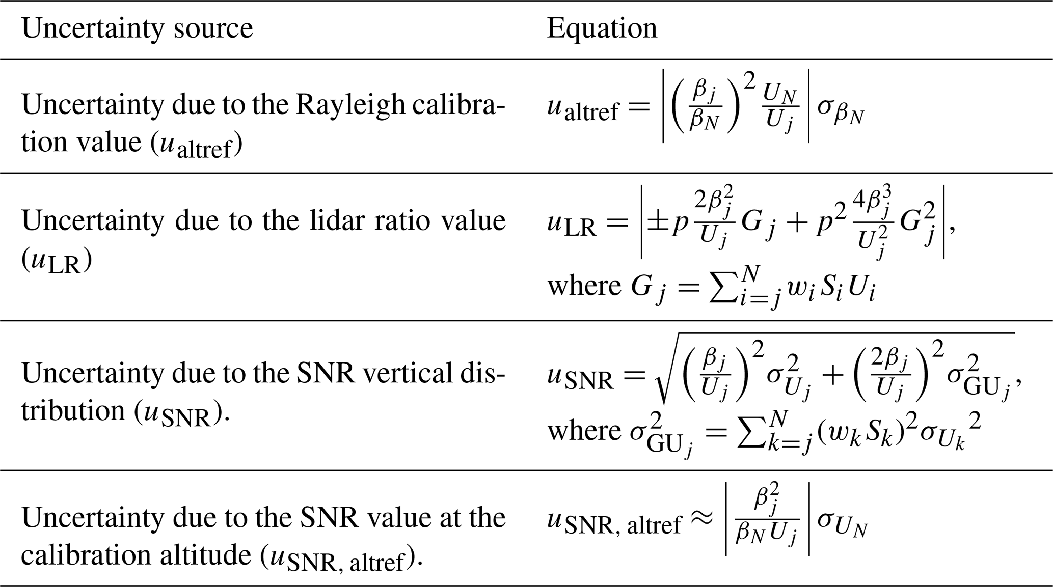
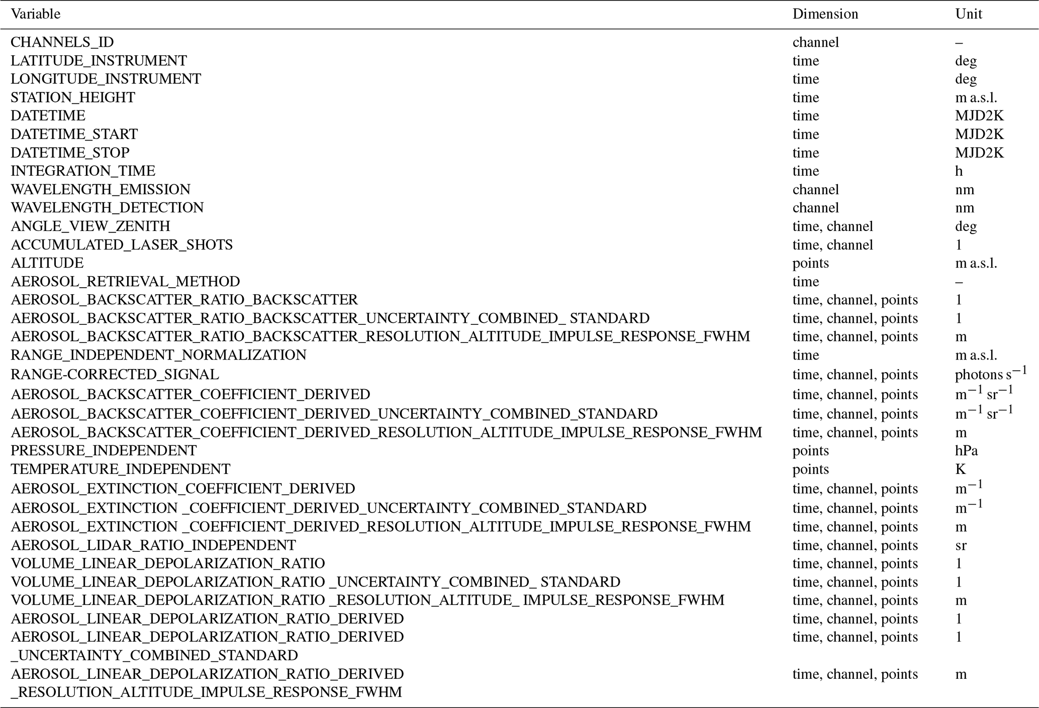
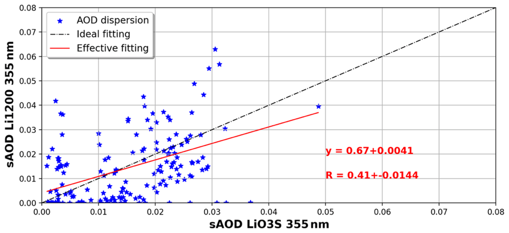
Figure D1 Dispersion of the AOD (10 to 17 km layer) at 355 nm between Li1200 and LiO3S. The black line represents the theoretical linear regression and the red line the actual linear regression.