the Creative Commons Attribution 4.0 License.
the Creative Commons Attribution 4.0 License.
 | 12 Sep 2024
Satellite-based near-real-time global daily terrestrial evapotranspiration estimates
Yong Luo
Jing M. Chen
Qiuhong Tang
Tammo Steenhuis
Wei Cheng
Wen Shi
Accurate and timely global evapotranspiration (ET) data are crucial for agriculture, water resource management, and drought forecasting. Although numerous satellite-based ET products are available, few offer near-real-time data. For instance, products like NASA's ECOsystem Spaceborne Thermal Radiometer Experiment mounted on the International Space Station (ECOSTRESS) and MOD16 face challenges such as uneven coverage and delays exceeding 1 week in data availability. In this study, we refined the Variation of the Standard Evapotranspiration Algorithm (VISEA) by fully integrating satellite-based data, e.g., European Centre for Medium-Range Weather Forecasts ERA5-Land shortwave radiation (which includes satellite remote sensing data within its assimilation system) and MODIS land surface data (which include surface reflectance, temperature and/or emissivity, land cover, vegetation indices, and albedo as inputs). This enables VISEA to provide near-real-time global daily ET estimates with a maximum delay of 1 week at a resolution of 0.05°. Its accuracy was assessed globally using observation data from 149 flux towers across 12 land cover types and comparing them with five other satellite-based ET products and Global Precipitation Climatology Centre (GPCC) data. The results indicate that VISEA provides accurate ET estimates that are comparable to existing products, achieving a mean correlation coefficient (R) of about 0.6 and an RMSE of 1.4 mm d−1. Furthermore, we demonstrated VISEA's utility in drought monitoring during a drought event in the Yangtze River basin in 2022 in which ET changes correlated with precipitation. The near-real-time capability of VISEA is, thus, especially valuable in meteorological and hydrological applications for coordinating drought relief efforts. The VISEA ET dataset is available at https://doi.org/10.11888/Terre.tpdc.300782 (Huang, 2023a).
- Article
(14688 KB) - Full-text XML
-
Supplement
(3449 KB) - BibTeX
- EndNote


Global terrestrial evapotranspiration (ET) is a vital component of Earth's water cycle and energy budget. It includes evaporation from the soil and water surfaces (some studies also consider evaporation from the intercepted precipitation in canopies) and plant transpiration (He et al., 2022; R. Wang et al., 2021; Zhang et al., 2021). Accurate and timely estimation of ET is essential for assessing changes in the water cycle under climate change quantitatively, monitoring drought vigilantly, and managing and allocating water resources effectively (Aschonitis et al., 2022; Han et al., 2021; Su et al., 2020).
Near-real-time ET estimation from reanalysis data has been widely used to assess ET changes in the global water cycle under different climate changes (Copernicus Climate Change Service, 2020). While these datasets, such as ERA5 (Albergel et al., 2012; Jarlan et al., 2008; Miller et al., 1992) and CRA-40 (Liu et al., 2023; Zhao et al., 2019), offer near-real-time latent heat flux (ET in energy units) with a delay of just 6 d, they typically have coarser spatial resolutions, often of 0.25° or more. This level of resolution may limit their effectiveness in detailed assessments of drought conditions and the optimization of water resource allocation. On the other hand, obtaining highly accurate, near-real-time, or real-time ET measurements through local eddy covariance or lysimeter methods can be very valuable (Awada et al., 2022), but collecting large-scale ET data on a fine grid using this equipment is prohibitively expensive (Barrios et al., 2015; Tang et al., 2009).
Satellite remote-sensing-based ET estimates outperform reanalysis data by providing high spatial resolution for detailed water utilization analysis, near-real-time data for prompt environmental response, and global coverage for comprehensive water cycle studies. These ET estimates rely on direct observations, enhancing accuracy (especially where ground data are sparse) and allowing for dynamic monitoring of land and vegetation changes.
The selected ET products discussed below have contributed significantly to estimating global ET and have gained recognition within the scientific community. The MOD16 ET product developed by Mu et al. (2007, 2011a) utilizes a Penman–Monteith-based approach and is driven by MODIS land cover, albedo, fractional photosynthetically active radiation, leaf area index, and daily meteorological reanalysis data from NASA's Global Modelling and Assimilation Office (GMAO) to estimate ET. The Advanced Very High Resolution Radiometer (AVHRR) ET product developed by Zhang et al. (2009, 2010) significantly advanced the study of the global water cycle. It employed a modified Penman–Monteith approach over land, integrated biome-specific canopy conductance determined by the normalized difference vegetation index (NDVI), and utilized a Priestley–Taylor approach over water surfaces. These algorithms were driven by the AVHRR Global Inventory Modeling and Mapping Studies (GIMMS) NDVI, daily surface meteorology data from National Centers for Environmental Prediction/National Center for Atmospheric Research (NCEP/NCAR) reanalysis, and solar radiation from the NASA/GEWEX Surface Radiation Budget Release 3.0. The FLUXCOM framework has made a substantial contribution to resolving the evapotranspiration paradox. It utilizes machine learning to integrate eddy covariance data from the global FLUXNET tower network, surface meteorological data from Climatic Research Unit (CRU) reanalysis, and remote sensing data (Jung et al., 2009, 2010, 2019). Additionally, the Global Land Evaporation Amsterdam Model (GLEAM), developed by Miralles et al. (2011b) and Martens et al. (2017), is one of the best satellite-based ET products using unique algorithmic approaches that have advanced the estimation of global ET and uses meteorological data from ERA5. Lastly, Penman–Monteith–Leuning Evapotranspiration V2 (PML), developed by Zhang et al. (2019, 2022), is the first to offer global ET coverage at a 500 m resolution, demonstrating high accuracy compared to local eddy covariance observations worldwide with MODIS satellite data and Global Land Data Assimilation System Version 2.1 (GLDAS-2.1) data (Zhang et al., 2023).
However, these ET products cannot provide near-real-time data due to reliance on local ground-based meteorology and land surface or reanalysis models, which are time-consuming to obtain globally. For example, MOD16 and PML use GMAO data and GLDAS-2.1, respectively. While AVHRR ET depends on AVHRR satellite data and NCEP/NCAR meteorology reanalysis data, GLEAM ET uses MODIS satellite data and ECMWF meteorology reanalysis data. FLUXCOM relies on FLUXNET and CRU reanalysis data, which are not updated in real time. Recently, NASA's ECOsystem Spaceborne Thermal Radiometer Experiment mounted on the International Space Station (ECOSTRESS) was designed to estimate global-scale ET (Fisher et al., 2019, 2020) thermal infrared data at 70 m resolution every 1 to 7 d. This results in uneven global coverage and reduced data frequency, especially in regions like the Middle East, as noted by Anderson et al. (2021) and Jaafar et al. (2022). In contrast, the Variation of the Moderate Resolution Imaging Spectroradiometer Standard Evapotranspiration Algorithm (VISEA) model only uses MODIS land products and ERA5-Land shortwave radiation, enabling near-real-time ET estimations.
The objective of this paper is twofold: (1) adapt the VISEA model for near-real-time, global application by replacing land-based solar radiation inputs with hourly shortwave radiation data from the ECMWF ERA5-Land data assimilation system (Muñoz Sabater, 2019) and (2) globally validate the model using a comprehensive collection of datasets, including meteorological instrument data and eddy covariance measurements from 149 FLUXNET towers (Pastorello et al., 2020). Additionally, multiyear ET datasets from GLEAM (Martens et al., 2017; Miralles et al., 2011), FLUXCOM (Jung et al., 2009, 2010, 2018), AVHRR (Zhang et al., 2009, 2010), MOD16 (Mu et al., 2007, 2011a), PML (Zhang et al., 2019, 2022), and precipitation from the Global Precipitation Climatology Centre (GPCC) (Schneider et al., 2011) are employed in the assessment.
2.1 Description of the VISEA algorithm
VISEA is a modification of the standard MODIS ET algorithm. The original MODIS algorithm, created by Mu et al. (2007, 2011a), was based on the Penman–Monteith method. VISEA introduces two significant modifications. First, it employs the vegetation (VI)–temperature (Ts) triangle method originally developed by Nishida et al. (2003) to estimate the air temperature. Second, VISEA incorporates hourly data on shortwave downward radiation from the ERA5-Land dataset to calculate daily average energy. These two advancements enable VISEA to estimate large-scale ET without needing local measurements as supplementary data.
This is unlike energy-budget-based ET algorithms, such as SEBS (Surface Energy Balance System), METRIC (Mapping Evapotranspiration at high Resolution with Internalized Calibration), and ALEXI (Atmosphere-Land Exchange Inverse), which calculate ET (latent heat flux) as the residual of the net radiation by subtracting soil heat flux and sensible heat flux. VISEA estimates ET using the Penman–Monteith equation, placing it in a different category of satellite-based global ET products currently in use. VISEA is a two-source model, which means that the ET in one grid cell was separated as the transpiration from the full vegetation cover and the evaporation from the bare soil surface if energy transfer from the vegetation to the soil surface was ignored (Nishida et al., 2003), i.e.,
where the subscript “veg” indicates the full vegetation cover and the subscript “soil” indicates the soil exposed to solar radiation (called bare soil). ETveg is the transpiration from the full vegetation cover area (W m−2), ETsoil is the evaporation from bare soil (W m−2), and fveg is the portion of the area with the vegetation cover, which can be calculated using the NDVI (calculation details are provided in Appendix A and Tang et al., 2009).
The available energy Q (W m−2), which is the sum of the latent heat flux and sensible heat flux (also known as the net radiation minus the soil heat flux), is also separated into the available energy for vegetation transpiration Qveg (W m−2) and Qsoil (W m−2) for bare soil evaporation, which was expressed by Nishida et al. (2003) as
As satellites like Terra and Aqua only provide instantaneous snapshot observations of Earth, a temporal scaling method is needed to convert instantaneous measurements into daily ET values. Nishida et al. (2003) used the satellite-based noontime instantaneous evaporation fraction (EF), defined as the ratio of the latent heat flux (ET) to the available energy as the daily EF (), and multiplied the daily Q to calculate the daily ET based on the assumption that the EF is constant over a day:
In the next section, we will detail how VISEA calculates the daily EF and Q in Eq. (3), daily air temperature, and daily land surface temperature.
2.1.1 Daily evaporation fraction calculation
Combining Eqs. (1)–(3), we calculated the instantaneous evaporation fraction EFi as
and are the instantaneous full vegetation coverage and bare soil EF, respectively. can be expressed as a function of instantaneous parameters (Nishida et al., 2003):
where α is the Priestley–Taylor parameter, which was set to 1.26 for wet surfaces (De Bruin, 1983). Δi is the instantaneous slope of the saturated vapor pressure, which is a function of the temperature (Pa K−1). γ is the psychometric constant (Pa K−1). is the instantaneous surface resistance of the vegetation canopy (s m−1). is the instantaneous aerodynamics resistance of the vegetation canopy (s m−1). was expressed by Nishida et al. (2003) as a function of the instantaneous soil temperature and the available energy based on the energy budget of the bare soil:
where is the instantaneous maximum possible temperature at the surface reached when the land surface is dry (K), is the instantaneous temperature of the bare soil (K), is the instantaneous air temperature, and is the instantaneous available energy for bare soil when is equal to (W m−2).
As the assumption of the noontime instantaneous evaporation fraction EFi equals the daily average evaporation fraction, EFd (i.e., EFi=EFd) caused a 10–30 % underestimation of daily ET (Huang et al., 2017; Yang et al., 2013), and we introduced a decoupling parameter to covert EFi to EFd (Huang et al., 2021; Tang et al., 2017; Tang and Li, 2017). The superscript “d” means “daily”, and the superscript “i” means “instantaneous”. This new decoupling-parameter-based evaporation fraction is developed from the Penman–Monteith and McNaughton–Jarvis mathematical equations:
where Ω is the decoupling factor that represents the relative contributions of radiative and aerodynamic terms to the overall evapotranspiration (Tang and Li, 2017), and is the value of the decoupling factor Ω for wet surfaces. Following Pereira (2004), the calculation details of Ω and Ω∗ are presented in Appendix B.
For full vegetation-covered areas, the decoupling-parameter-based daily is expressed as
where is the instantaneous canopy resistance (s m−1), and is the instantaneous aerodynamic resistance (s m−1). The process of determining these resistances is presented in Appendix C. For bare soil, the decoupling-parameter-based daily is calculated as
Thus, EFd is expressed as
The same energy balance equations are used to calculate the instantaneous values Qi, , and and the daily values Qd, , and , but with the parameters adjusted for each time frame. The details of the calculation of the daily values are outlined below.
2.1.2 Daily calculation of available energy and
We used an improved daily available energy Q (W m−2) method (Huang et al., 2023) for the vegetation, and the bare soil surface is calculated using the energy balance equation:
where Rn is the net radiation (W m−2), which could be calculated using the land surface energy balance. G is the soil heat flux (W m−2) G≈0 on a daily basis (Fritschen and Gay, 1979; Nishida et al., 2003; Tang et al., 2009):
where albedod is the daily albedo of the soil surface. is the daily incoming shortwave radiation (W m−2) obtained from the ERA5_Land shortwave radiation (called ERA5_Rd). and are the daily emissivity of the land surface and atmosphere. σ is the Stefan–Boltzmann constant. is the daily near-surface air temperature (K). is the daily surface temperature (K). The difference from the former study by Huang et al. (2021) is that and were not made equal. Instead, we calculated using the methods of Brutsaert (1975) and Wang and Dickinson (2013) as detailed in Appendix D. was retrieved from MOD11C1.
We account for the influence of clouds by assuming a linear correlation between downward longwave radiation and cloud coverage in the calculation of downward longwave radiation based on the study of Huang et al. (2023):
where Cloudd is the daily clearness index and Kt is (Chang and Zhang, 2019; Goforth et al., 2002)
where is the daily extraterrestrial radiation calculated using the FAO (1998).
can be calculated by assuming according to the VI–Ts method, which implies that the minimum land surface temperature occurs in fully vegetated grid cells and is equivalent to (Huang et al., 2023). According to the land surface energy budget, the daily available energy of the vegetation coverage area and the bare soil can be calculated following the study of Huang et al. (2023):
The daily mean air temperature can be extended by sine and cosine functions based on the instantaneous air temperature , which was calculated using the linear correlation in the VI–Ts method. Thus, is the daily downward longwave radiation (W m−2) and is the daily upward longwave radiation (W m−2), where CG is an empirical coefficient ranging from 0.3 for a wet soil to 0.5 for a dry soil (Idso et al., 1975).
and are calculated using the energy balance equations, which are robust on both instantaneous and daily scales. Thus, instantaneous and are calculated using the same set of Eqs. (17) and (18) by replacing the daily parameters with the instantaneous parameters.
Following the study of Huang et al. (2023), the daily ETd can be calculated using the daily EFd and Qd as
Figure 1 illustrates the workflow of VISEA. VISEA utilizes land cover data from the International Geosphere-Biosphere Programme (IGBP) MOD12C1 land cover classification. When land cover in an IGBP MOD12C1 data grid cell is identified as a water surface, VISEA uses the Priestley–Taylor equation to compute water surface evaporation. This process guarantees that the unique attributes of water surfaces are precisely reflected in VISEA ET calculations.
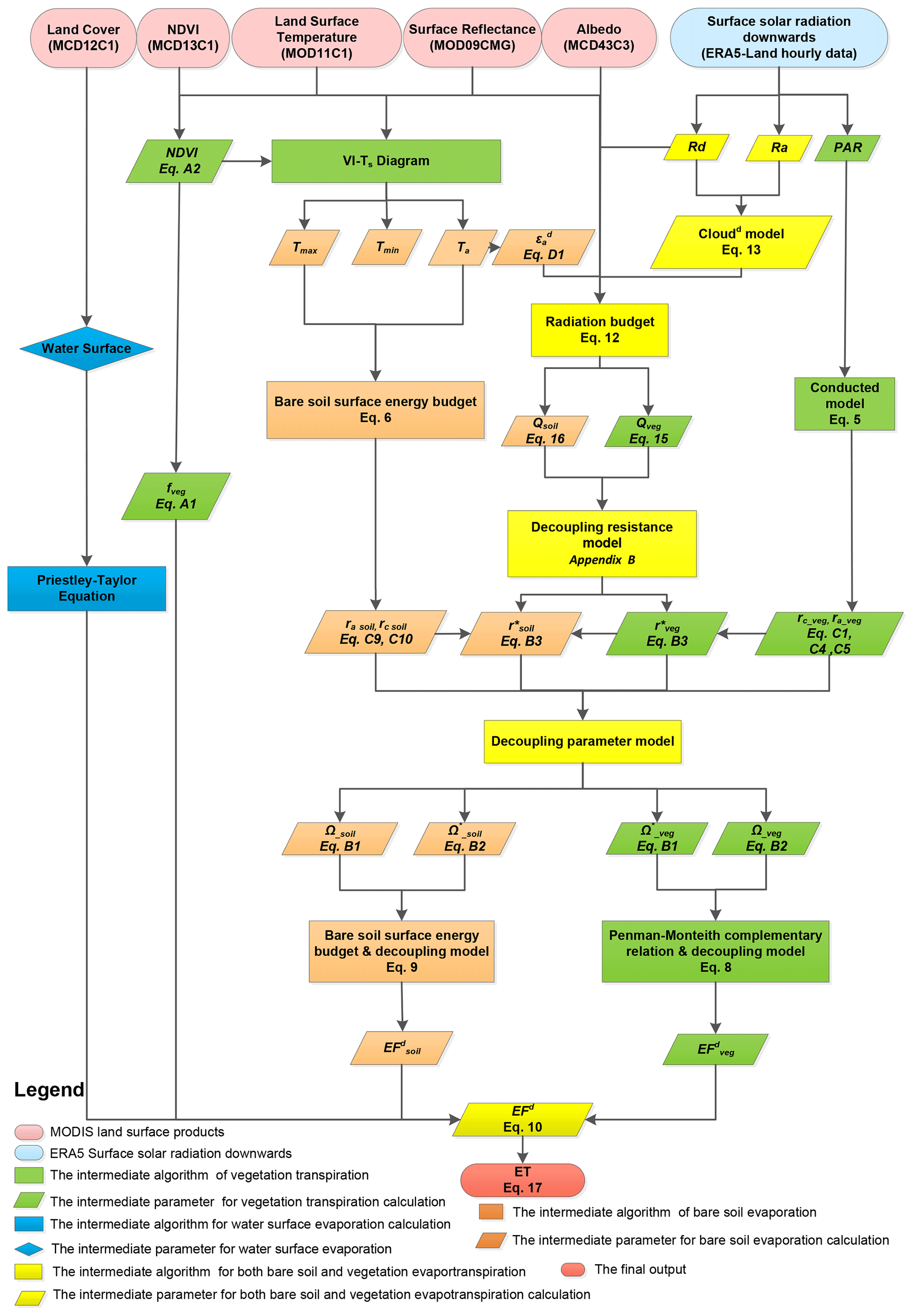
Figure 1Schematic of the VISEA algorithm. The ovals in the top row are the databases, the square boxes are the algorithms, and the parallelograms are the parameters. The numbers in the parentheses are the equations to determine the parameters.
2.1.3 The calculation of daily air temperature and surface temperature
Daily air temperature is a critical parameter in the VISEA algorithm and is used in calculations for downward longwave radiation, daily aerodynamic resistance, and surface resistance. The key innovation in calculating involves the VI–Ts method to estimate the instantaneous air temperature during the daytime (Huang et al., 2017; Nishida et al., 2003; Tang et al., 2009).
The VI–Ts method was developed based on the empirical linear relationship between the Ts and the VI. The surface temperature increases when the vegetation index decreases, and conversely the surface temperature decreases when the vegetation index increases. In the scatterplot, defined by the VI (horizontal axis) and Ts (vertical axis) from the neighboring 5×5 grid cells, we identify the “warm edge” (characterized by a low vegetation cover fraction and a high Ts) and the “cold edge” (characterized by a high vegetation cover fraction and a low Ts). The warm edge is automatically selected as the hypotenuse of the triangle formed by these scatter points. Through simple interpolation, a Ts corresponding to any given vegetation condition in the range of the warm edge and cold edge can be determined. The lowest Ts can be determined by the highest VI, and the highest Ts can be determined by the lowest VI. Therefore, following Nishida et al. (2003) and assuming that the lowest surface temperature equals the air temperature (Ta), we can derive the daily air temperature.
For the nighttime periods, it is assumed that air temperature is equivalent to the nighttime land surface temperature provided by MOD11C1. These two temperature estimates are then extended to hourly air temperature profiles using a sine–cosine fitting curve. The 24 h average of is used as . Similarly, is calculated using MOD11C1 land surface temperature data for both daytime and nighttime. These estimates are extended to hourly surface temperature profiles using a similar sine–cosine fitting curve, and the daily average of is determined (Huang et al., 2021).
This VI–Ts method allows for the estimation of and without the need for additional meteorological data. However, some studies have found that the VI–Ts method may not consistently provide satisfactory results, especially in colder regions where vegetation thrives better at higher temperatures.
2.2 Technical validation
The correlation coefficient, RMSE, and Nash–Sutcliffe efficiency are used to evaluate our global daily ET estimates with eddy covariance measurements and compared with the other five independent global ET products on a monthly scale.
The correlation coefficient R is calculated as
R is the correlation coefficient. X is the estimated variable. is the average of X. Y is the observed variable. is the average of Y.
The RMSE is calculated as
For a more nuanced understanding of the RMSE, we have deconstructed it into two distinct components: RMSEs (systematic RMSE) and RMSEu (unsystematic RMSE). This breakdown allows a more detailed examination of the systematic and unsystematic sources contributing to the overall error metric.
The systematic RMSEs is calculated as
The unsystematic RMSEu is calculated as
where , and a and b are the least-squares regression coefficients of the estimated variable Xi and the observed variable Yi. N is the sample size (Norman et al., 1995).
The Nash–Sutcliffe efficiency (NSE) coefficient is
The ratio of the standard deviations of X and Y are
The bias of X and Y is
2.3 The gap-filling of MODIS data
MODIS sensors on board Terra and Aqua observe Earth twice a day. However, there are always data gaps in the MODIS land products because of cloud cover problems. In the VISEA algorithm, we used the data from the neighboring days to fill the data gaps. The periods when MODIS land temperature data were missing, primarily due to cloud cover, accounted for approximately one-third of the observation period. The accuracy of this gap-filling method is evaluated in Sect. 4.
3.1 The input data
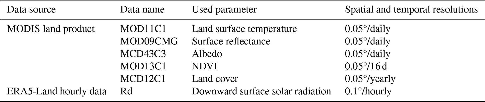
The input data include the MODIS land products: daily 0.05° surface reflectance (MOD09CMG), land surface temperature and emissivity (MOD11C1) and albedo (MCD43C3), 8 d 0.05° vegetation indices (MOD13C1), and yearly 0.05° land cover products (MCD12C1). We also used hourly downward surface solar radiation from the Fifth Generation of the European Centre for Medium-Range Weather Forecasts (ECMWF) Reanalysis (ERA5), i.e., “ERA5-Land hourly data from 1950 to present” data, as the energy input of the VISEA algorithm. The surface solar radiation data from ERA5-Land and the land data products from MODIS are both near-real-time datasets with a 1-week delay, enabling VISEA to provide global near-real-time ET estimations. Details of the input data, their download links, the variable names, the used parameters, and the spatial and temporal resolutions are given in Table 1.
3.2 The evaluation data
3.2.1 The flux tower measurements from FLUXNET
We evaluated the accuracy of the input ERA5-Land shortwave radiation, estimated daily net radiation, air temperature, and ET by comparing them with measurements from FLUXNET2015 (Pastorello et al., 2020). FLUXNET consists of 212 globally distributed flux towers, and it has implemented quality control measures for energy closure and is considered reliable (Baldocchi et al., 2001; Pastorello et al., 2020; Wang et al., 2022). The data from FLUXNET2015 can be obtained at https://fluxnet.org/data/download-data (last access: 12 May 2023). We selected data from 2001 to 2015 and excluded sites with zero ERA5-Land downward shortwave radiation.
While there are records from 212 flux towers in our datasets, not all met the stringent inclusion criteria. Each site needed to fulfill three specific requirements to be included in our analysis: (1) availability of data for the period spanning 2001 to 2015; (2) ERA5-Land downward shortwave radiation greater than 0 within the 0.1°×0.1° grid cell corresponding to the flux tower's location; and (3) conformity with MODIS land cover data (MOD12C1) at the 0.05°×0.05° grid cell level, ensuring that the flux tower was situated on land rather than over the ocean. Based on these criteria, we selected a subset of 149 flux towers that met these stringent criteria. This approach ensures the reliability and relevance of our analysis. The distribution of these 149 flux towers is presented in Fig. 2. Table S1 in the Supplement shows the longitude, latitude, elevation, and land cover type (classified by the IGBP) of these sites. The 149 sites covered 12 IGBP land cover types: 18 croplands (CRO), 1 closed shrubland (CSH), 15 deciduous broadleaf forests (DBF), 1 deciduous needleleaf forest (DNF), 10 evergreen broadleaf forests (EBF), 34 evergreen needleleaf forests (ENF), 30 grasslands (GRA), 5 mixed forests (MF), 8 open shrublands (OSH), 8 savannas (SAV), 13 wetlands (WET), and 6 woody savannas (WSA).
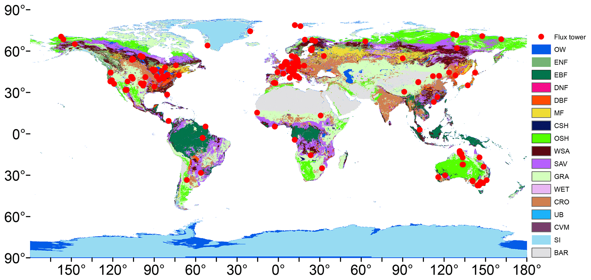
Figure 2The distribution of the 149 flux towers from FLUXNET in different IGBP land cover types, specifically OW (water bodies), ENF (evergreen needleleaf forests), EBF (evergreen broadleaf forests), DNF (deciduous needleleaf forests), DBF (deciduous broadleaf forests), MF (mixed forests), CSH (closed shrublands), OSH (open shrublands), WSA (woody savannas), SAV (savannas), GRA (grasslands), WET (permanent wetlands), CRO (croplands), UB (urban and built-up lands), CVM (cropland and natural vegetation mosaics), SI (snow and ice), and BAR (barren).
3.2.2 The other gridded ET and precipitation products
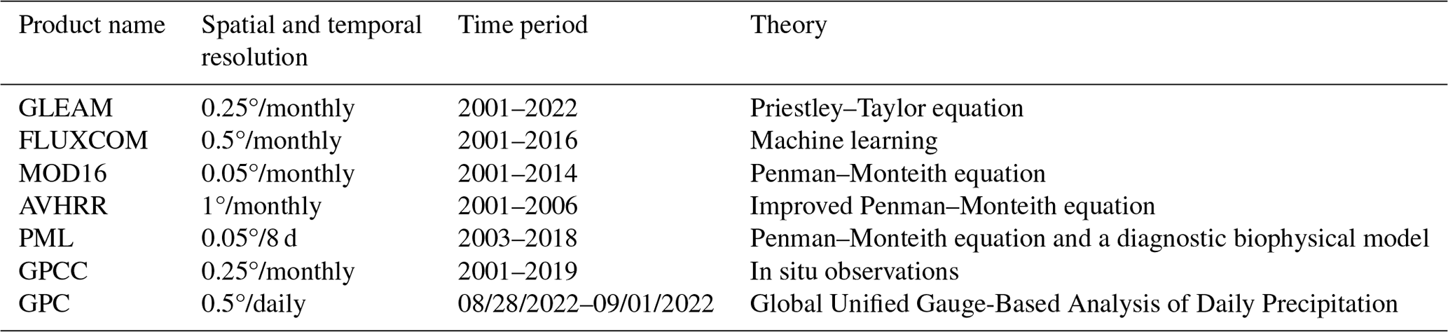
Five independent globally gridded ET products and one precipitation product were used to evaluate VISEA-estimated ET. The five ET products include two MODIS-based ET products, i.e., MOD16 (Mu et al., 2007, 2011a) and PML (Zhang et al., 2019, 2022), one AVHRR-based ET (Zhang et al., 2009, 2010), one machine learning algorithm output, the FLUXCOM ET data (Jung et al., 2009, 2010, 2018, 2019), and one multi-satellite data-based GLEAM ET (Martens et al., 2017; Miralles et al., 2011). The precipitation data were from GPCC, which is based on local measurements (Becker et al., 2013; Schneider et al., 2014, 2017) and the Global Unified Gauge-Based Analysis of Daily Precipitation (GPC). Details of these five ET products and the precipitation data are given in Table 2. To maintain the consistency of the temporal and spatial resolutions for comparison purposes, we obtained the monthly MOD16 and PML despite their original temporal resolution of 8 d. We used the 0.05°×0.05° version of MOD16, AVHRR ET, and PML. Additionally, for multiyear-scale comparisons, we confined our dataset to the time frame between 2001 and 2020. This selection enabled us to utilize a diverse range of ET products, effectively minimizing the influence of temporal discrepancies on our comparative analysis. We also incorporated daily ET data from GLEAM and VISEA alongside precipitation data from the Climate Prediction Center (CPC) from 25 July to 2 August 2022. This allowed for near-real-time analysis of ET and precipitation during the Yangtze River drought incident within that interval, despite the datasets potentially encompassing more extensive periods.
Table 2The five global gridded ET products and the one precipitation product used for comparison with our near-real-time global daily terrestrial ET estimates.
To evaluate the performance of ERA5_Rd across different land cover initial categories, we juxtaposed downward solar radiation input data from ERA5-Land (ERA5_Rd) with measurements obtained from 149 flux towers (Obv_Rd) across diverse IGBP land cover types, as illustrated in Fig. 3. The results indicate commendable agreement between ERA5_Rd and Obv_Rd measurements for the majority of land covers, with notable exceptions observed in SAV. Specifically, the mean NSE is 0.84, the mean R is 0.92, and the RMSE is 38.3 W m−2.
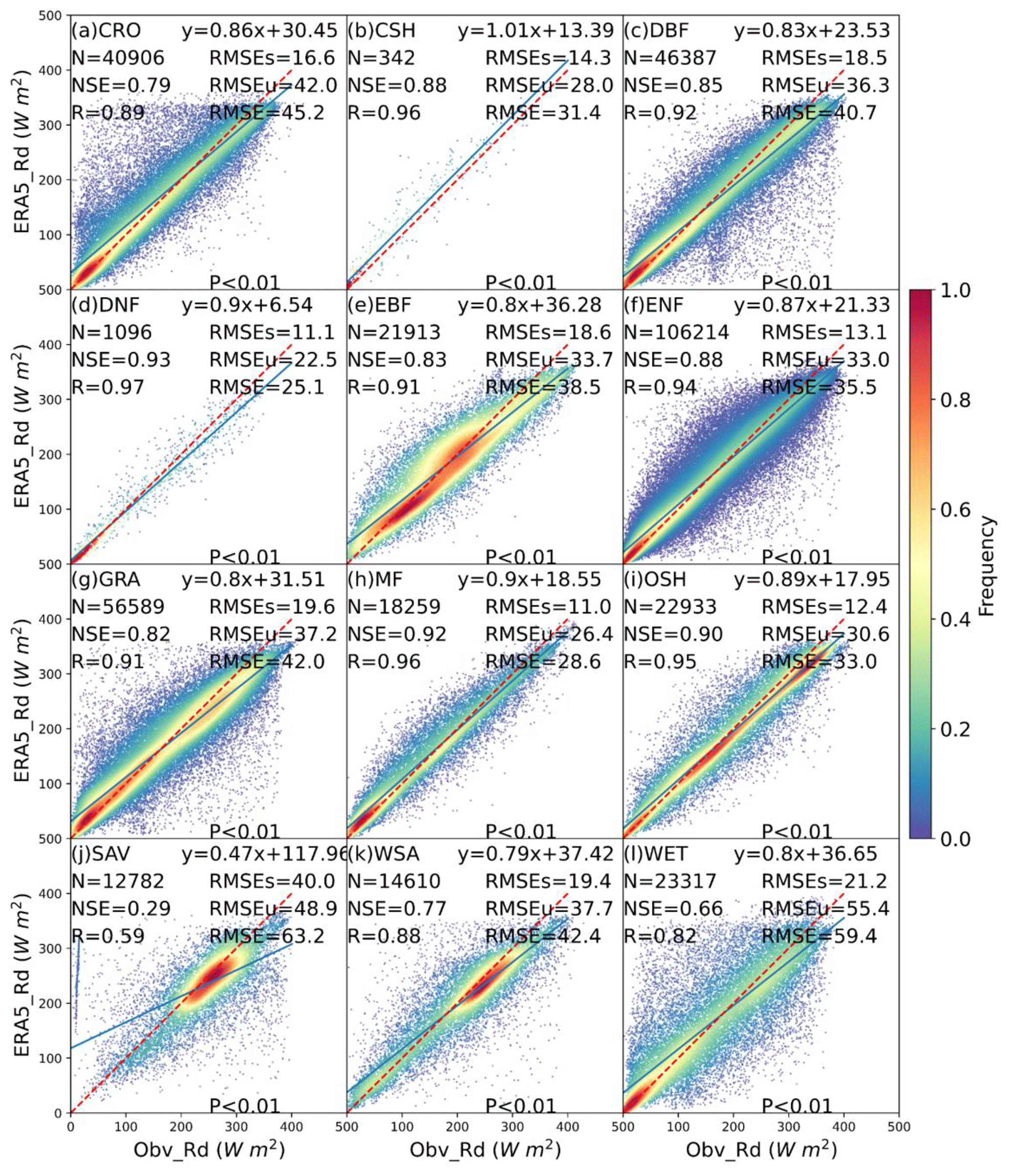
Figure 3The scatterplot of downward solar radiation from ERA5-Land (ERA5_Rd) compared with local instrument measurements (Obv_Rd) in 12 IGBP land cover types: CRO, CSH, DBF, DNF, EBF, ENF, GRA, MF, OSH, SAV, WSA, and WET. The red dotted line is the 1:1 line. N is the number of data points, NSE is the Nash–Sutcliffe efficiency, R is the correlation coefficient, RMSE is the root mean square error, RMSEs is the systematic RMSE, and RMSEu is the unsystematic RMSE. The frequency denotes the probability density estimated using the kernel density estimation (KDE) method with a Gaussian kernel, and it is then scaled to ensure that the maximum value of the probability density function equals 1. P is the P value for the correlation coefficient.
Figure 3 shows that ERA5 input shortwave radiation generally agrees well with local measurements. ERA5_Rd exhibits optimal performance in DNF and MF, which is reflected by NSE and R values surpassing 0.9. In these land covers, the mean RMSEs is 11 W m−2, the mean RMSEu is 24.5 W m−2, and the mean RMSE is 26.9 W m−2. However, its performance in SAV is notably sub-par and characterized by an NSE of 0.29, an R of 0.59, the highest RMSEs of 40 W m−2, an RMSEu of 48.9 W m−2, and an RMSE of 63.2 W m−2. For ERA5_Rd, the mean RMSEs amounts to 16 W m−2 and the mean RMSEu is 34.8 W m−2, suggesting that ERA5_Rd demonstrates high accuracy by effectively capturing the systematic variation in Obv_Rd, as indicated by its relatively low RMSEs and RMSEu close to the RMSE (Willmott, 1981) in most land covers, except for SAV. Specifically, in Fig. 3, the Rd is derived from ERA5 exhibits very low P values (<0.01).
Several factors come into play in understanding the disparities in performance in ERA5_Rd across different land cover types. In regions characterized by denser forests, such as DNF and MF, ERA5_Rd's good performance may be attributed to the lower density of ground-based meteorology stations (DNF, N=1096) and the relatively uniform subsurface and canopy coverage in MF, facilitating a more accurate representation in the ERA5 radiative transfer model. Conversely, savannas present unique challenges due to their sparse vegetation and flat terrain, influencing sunlight transmission dynamics (Yang and Friedl, 2003). Land use changes, including farming and urban development, further complicate the accuracy of sunlight transmission. Additionally, factors like aerosols from natural or anthropogenic sources contribute to data variations (Naud et al., 2014; Y. Wang et al., 2021). The inaccuracies in accounting for the rainy season, leading to increased cloud cover and rainfall in savannas, contribute to ERA5_Rd's limitations (Jiang et al., 2020).
We chose to utilize 0.05° MODIS data for their detailed land surface information, daily time step, and global coverage, which are essential for accurate and near-real-time ET calculations. Although ERA5 data have a coarser 0.1° resolution, they provide necessary atmospheric inputs that can be effectively interpolated to match the MODIS resolution without significant loss of accuracy. As illustrated in Figs. 3 and 4, our tests confirm that this method achieves accurate ET despite the resolution differences.
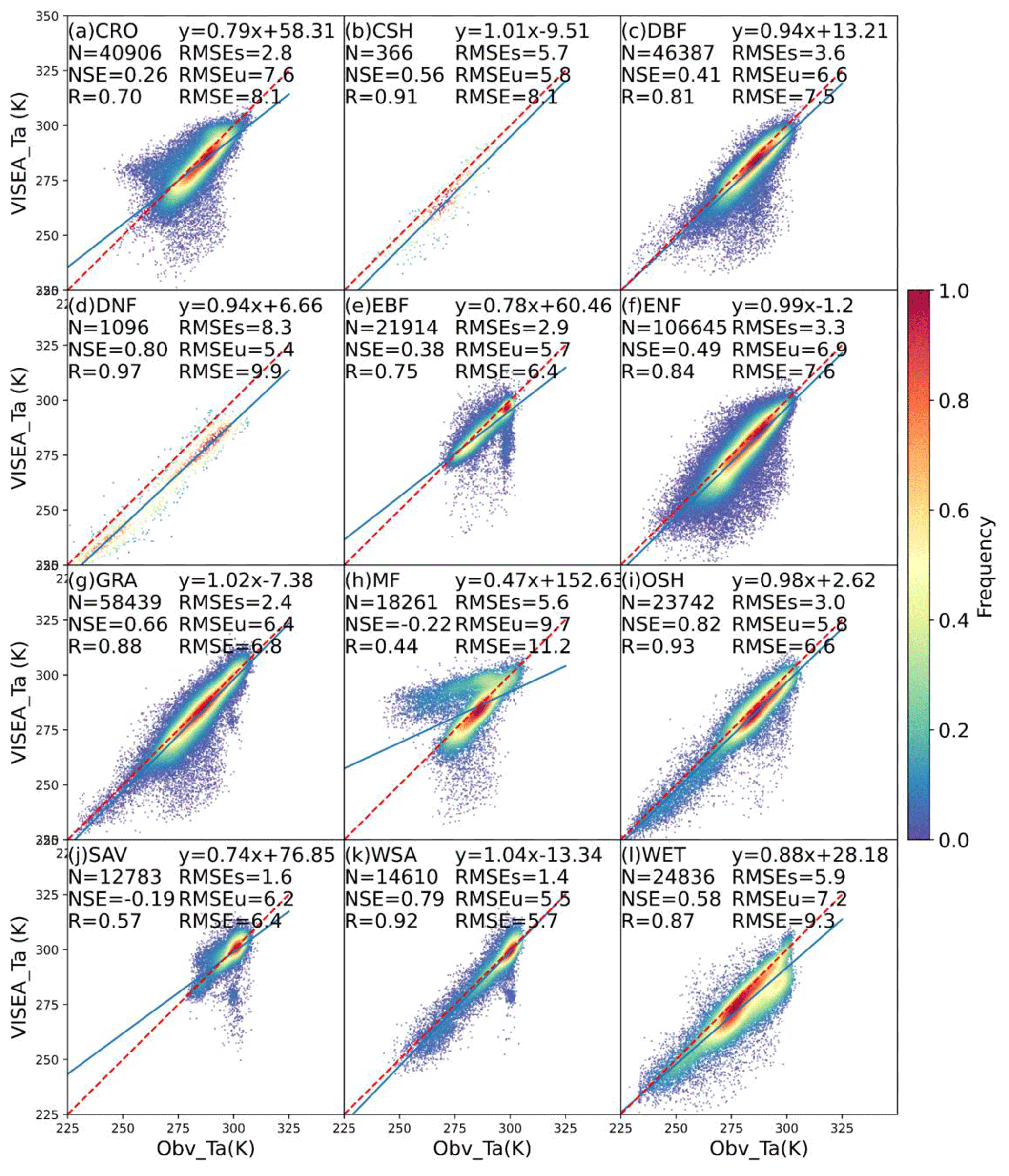
Figure 4The scatterplot of daily air temperature simulated by VISEA (VISEA_Ta) compared with local instrument measurements (Obv_Ta) in 12 IGBP land cover types: CRO, CSH, DBF, DNF, EBF, ENF, GRA, MF, OSH, SAV, WSA, and WET. The red dotted line is the 1:1 line. N is the number of data points, NSE is the Nash–Sutcliffe efficiency, R is the correlation coefficient, RMSE is the root mean square error, RMSEs is the systematic RMSE, and RMSEu is the unsystematic RMSE. The frequency denotes the probability density estimated using the KDE method with a Gaussian kernel, and it is then scaled to ensure that the maximum value of the probability density function equals 1.
Figure 4 depicts scatterplots illustrating the comparison between the estimated air temperature using the VI–Ts method (VISEA_Ta) and local meteorological measurements (Obv_Ta). The analysis reveals that VISEA_Ta generally aligns with Obv_Ta, exhibiting NSE values ranging from −0.22 (MF) to 0.82 (OSH), R values ranging from 0.44 (MF) to 0.97 (DNF), and RMSE values ranging from 5.7 K (WSA) to 11.2 K (MF). Particularly noteworthy is VISEA_Ta's outstanding performance in OSH (NSE=0.82, R=0.93, RMSE=6.6 K), WSA (NSE=0.79, R=0.92, RMSE=5.7 K), and GRA (NSE=0.66, R=0.88, RMSE=6.8 K). Conversely, the least satisfactory performance is evident in MF (, R=0.44, RMSE=11.2 K), SAV (, R=0.57, RMSE=6.4 K), and CRO (NSE=0.26, R=0.70, RMSE=8.1 K). The RMSEs is lower than the RMSEu at most of the land cover sites, except in DNF. Despite VISEA_Ta displaying a high NSE of 0.8 and an R of 0.97 in DNF, it exhibits a higher RMSEs (8.3 K) compared to the RMSEu (5.4 K), indicating a systematic underestimation of VISEA_Ta in DNF.
As detailed in Sect. 2.4, the VI–Ts method relies on a negative correlation between the VI and the Ts, which is ideally suited for cases with significant VI and Ts differences. However, the assumed negative correlation breaks down for land cover types like DNF and MF in temperate regions with distinct seasons and cool to cold climates. In these regions, the positive correlation between the VI and Ts, driven by vegetation growth proportional to a rising Ts, results in the failure of the VI–Ts method. The challenges persist in SAV, where the VI–Ts method encounters difficulties during the dry and wet seasons. In the dry season, the method falters due to the prevalence of bare soil, resulting in VI values approaching 0 and homogeneously high Ts values. Conversely, the wet season presents challenges, with both the VI and Ts exhibiting relatively high values and limited variances between the grid cells, ultimately undermining the accuracy of VISEA_Ta estimation.
The simulated daily net radiation (VISEA_Rn) from VISEA is assessed against local meteorological measurements (Obv_Rn) in Fig. 5. In contrast to the satisfactory performance of ERA5_Rd in Fig. 3, VISEA_Rn exhibits more notable discrepancies characterized by significant underestimation compared to Obv_Rn. This is reflected in the mean NSE of 0.49, mean R of 0.74, and mean RMSE of 43.3 W m−2. Specifically, VISEA_Rn demonstrates good accuracy in certain land cover types, including CHS with an NSE of 0.67, an R of 0.84, and an RMSE of 29.7 W m−2; EBF with an NSE of 0.63, an R of 0.8, and an RMSE of 42.9 W m−2; and ENF with an NSE of 0.66, an R of 0.83, and an RMSE of 39.6 W m−2. However, its performance notably diminishes in OSH, where it records an NSE of 0.16, an R of 0.61, and an RMSE of 56 W m−2, as well as in SAV, with an NSE of 0.21, an R of 0.52, and an RMSE of 44.2 W m−2. While VISEA_Rn appears to have lower accuracy compared to ERA5_Rd, in the majority of the land cover types, the RMSEs is smaller than the RMSEu, with a mean RMSEs of 25.2 W m−2 and a mean RMSEu of 34.3 W m−2. Moreover, the RMSEu of 43.3 W m−2 is almost the same as the RMSE.
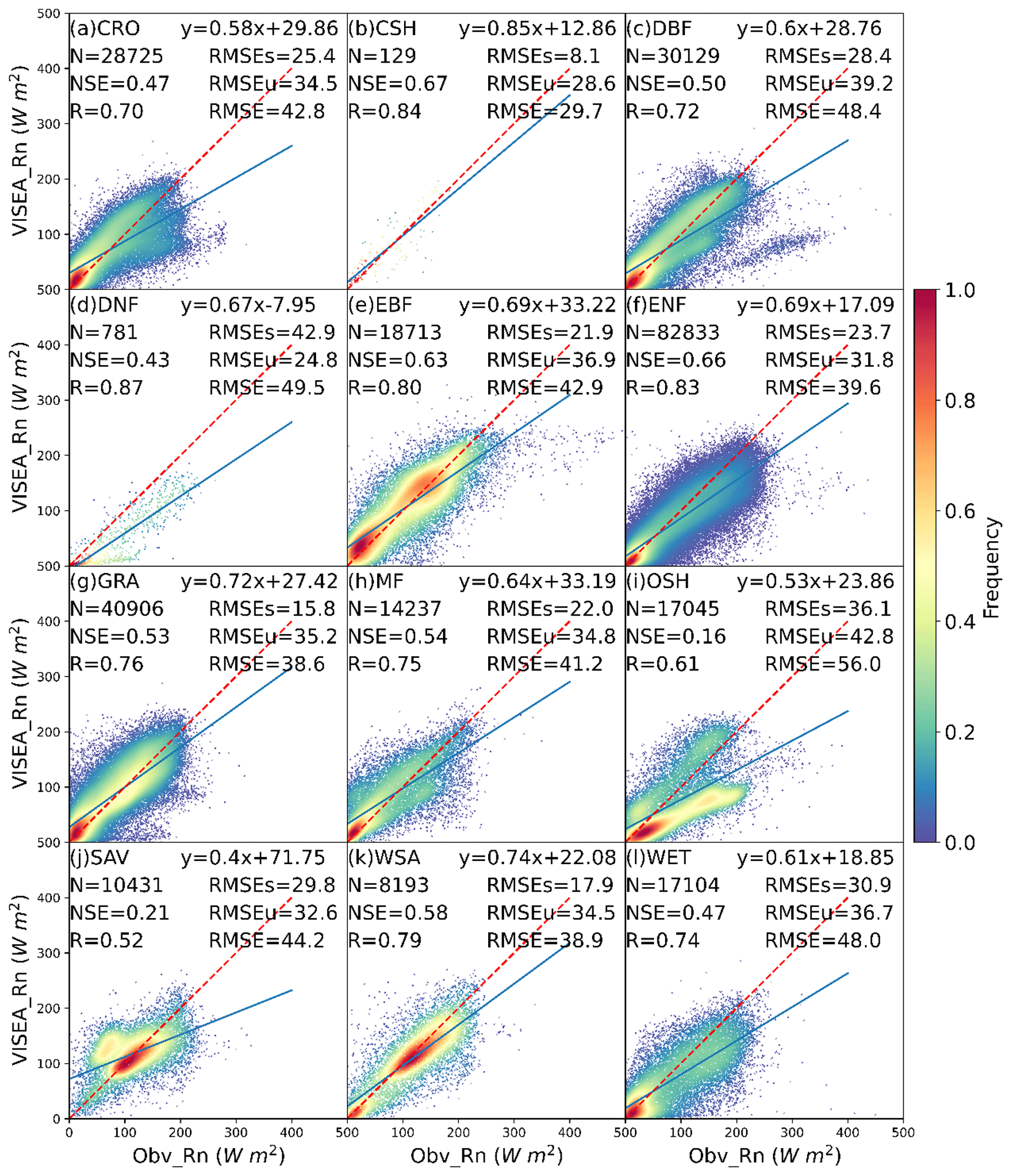
Figure 5The scatterplot of daily net radiation simulated by VISEA (VISEA_Rn) compared with local instrument measurements (Obv_Rn) in 12 IGBP land cover types: CRO, CSH, DBF, DNF, EBF, ENF, GRA, MF, OSH, SAV, WSA, and WET. The red dotted line is the 1:1 line. N is the number of data points, NSE is the Nash–Sutcliffe efficiency, R is the correlation coefficient, RMSE is the root mean square error, RMSEs is the systematic RMSE, and RMSEu is the unsystematic RMSE. The frequency denotes the probability density estimated using the KDE method with a Gaussian kernel, and it is then scaled to ensure that the maximum value of the probability density function equals 1.
In the context of VISEA_Rn, a consistent pattern of approximately 30 % underestimation of net radiation across various land cover types raises noteworthy discussions. This systematic discrepancy could be linked to the disparity in vegetation coverage between the observed sites' footprint and the mean vegetation coverage of the 0.05°×0.05° grid cell. Specifically, the lower albedo within the footprint, compared to the grid cell's average albedo (as expressed by Eq. 14), contributes to the underestimation of Obv_Rn. This is particularly evident in OSH, where the vegetation coverage within the footprint significantly exceeds the mean vegetation coverage of the grid cell (<0.2 compared to >0.5). Factors such as the bias in ERA5_Rd (refer to Fig. 3j) and VISEA_Ta (refer to Fig. 4j) contribute to the underestimation of VISEA_Rn in SAV. Moreover, a substantial 50 % underestimation of the DNF results from the underestimated VISEA_Ta (refer to Fig. 4d) leads to a subsequent underestimation of downward longwave radiation.
Figure 6 illustrates scatterplots of daily ET simulated by VISEA (VISEA_ET) against eddy covariance measurements obtained from 149 flux tower sites (Obv_ET) in 12 IGBP land cover types. The scatterplots of VISEA_ET reveal a dispersed distribution, as evidenced by an average NSE of −0.08, an average R of 0.56, and an average RMSE of 1.4 mm d−1. Notably, VISEA_ET tends to underestimate daily ET across most of the land cover types. Of the 12 land cover types, VISEA_ET exhibits the highest accuracy in DNF, with an NSE of 0.4, an R of 0.82, and an RMSE of 0.9 mm d−1. This was closely followed by GRA, with an NSE value of 0.26, an R value of 0.65, and an RMSE value of 1.3 mm d−1. However, for the CRO, ENF, and WET land cover types, the NSE values, while above 0, are close to 0 (mean NSE of 0.11), with a mean R of 0.53 and a mean RMSE of 1.3 mm d−1. In the remaining land cover types, particularly in OSH and SAV, VISEA_ET appears to struggle when aligning with local measurements, resulting in NSE values of −0.57 and −0.51, R values of 0.31 and 0.36, and RMSE values of 1.2 and 1.7 mm d−1, respectively. With the evaluation of daily VISEA_ET with observed ET (Obv_ET) in CRO and WET, the bias mainly comes from the bias in ERA5_Rd (the third highest RMSE of 45.2 W m−2 and the second highest RMSE of 59.4 W m−2) (Fig. 3a and l). In ENF, the biases are primarily caused by the inability of VISEA_ET to capture Obv_ET in a cold climate, with low net radiation estimation (Fig. 5f) and air temperature (Fig. 4f). For OSH, the bias mainly arises from the poor estimation of VISEA_Rn, which has the lowest NSE of 0.16 and the highest RMSE of 56 W m−2 (Fig. 5i). The bias of VISEA_ET in SAV is a result of the combined biases in ERA5_Rd (the lowest NSE and R values of 0.29 and 0.59, respectively, and the highest RMSE of 63.2 W m−2) and VISEA_Ta (the second lowest NSE and R values of −0.19 and 0.57, respectively).
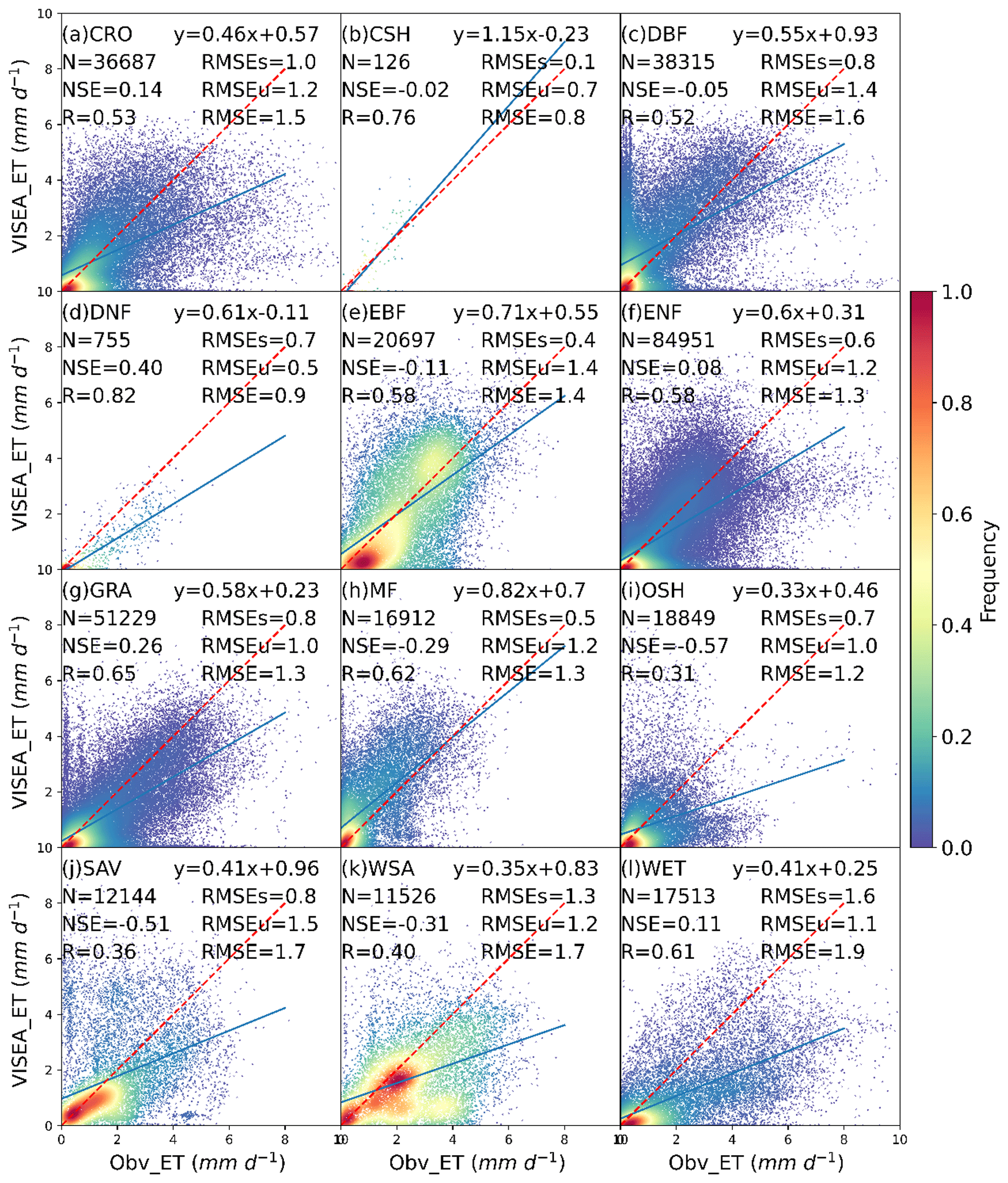
Figure 6The scatterplot of daily ET simulated by VISEA (VISEA_ET) compared with local instrument measurements (Obv_ET) in 12 IGBP land cover types: CRO, CSH, DBF, DNF, EBF, ENF, GRA, MF, OSH, SAV, WSA, and WET. The red dotted line is the 1:1 line. N is the number of data points, NSE is the Nash–Sutcliffe efficiency, R is the correlation coefficient, RMSE is the root mean square error, RMSEs is the systematic RMSE, and RMSEu is the unsystematic RMSE. The frequency denotes the probability density estimated using the KDE method with a Gaussian kernel, and it is then scaled to ensure that the maximum value of the probability density function equals 1.
The periods when MODIS land temperature data were missing, primarily due to cloud cover, accounted for approximately one-third of the observation period. Using the gap-filling method (Sect. 2.3), it can be observed that, for most surfaces, the accuracy of VISEA was not significantly affected by clouds, as evidenced by the figures below. The accuracy on cloudy days is slightly lower for some surfaces compared to clear days. For example, in the case of DBF, the correlation coefficient R is 0.52 on both clear and cloudy days and the RMSE is 1.4 mm d−1 on both clear and cloudy days, indicating a slight decrease in accuracy under cloudy conditions. Similarly, for ENF, the R value is 0.59 on clear days and 0.56 on cloudy days. At the same time, the RMSE is 1.3 mm d−1 on clear days and 1.4 mm d−1 on cloudy days, showing that, although there is some impact, the overall performance of VISEA remains robust across different weather conditions (Figs. S4 and S5 in the Supplement).
We also tested the VISEA sensitivity to different radiation input data by comparing results obtained using the CERES and ERA5 datasets. Specifically, we analyzed the performance of the VISEA model in simulating net radiation (Rn) and ET, comparing these simulations with ground-based observational data. Figures S1 and S2 in the Supplement compare the downward shortwave radiation data from CERES and ERA5 with ground-based observations of the 149 flux towers. The CERES shortwave radiation data generally agree with the observational data, with a mean R of 0.89, a mean RMSE of 34.8 W m2, and a mean NSE of 0.78. In contrast, the ERA5 shortwave radiation data have a mean R of 0.85, a mean RMSE of 40.4 W m2, and a mean NSE of 0.58 when compared with the ground-based observations, indicating systematic bias and lower precision for the ERA5 net radiation compared with CERES. Figures S2 and S5 in the Supplement compare the net radiation of the flux towers with that calculated using the VISEA model with shortwave radiation of CERES and ERA5 as input data. For the CERES data, the mean R is 0.74, the mean RMSE is 34.3 W m2, and the mean NSE is 0.64. The ERA5 data yield a mean R of 0.64, a mean RMSE of 39.44 W m2, and a mean NSE of 0.44. Finally, the ET calculated with VISEA using the net radiation of CERES and ERA5 as input is compared with ground-based data in Figs. S3 and S6 in the Supplement. Again, CERES outperforms ERA5, as indicated by the statistical measures. The sensitivity analysis reveals that the VISEA model's performance depends greatly on the quality of the incident radiation data used as input. The model shows better accuracy and consistency with CERES data than with ERA5 data. Therefore, selecting high-precision radiation data is crucial for improving the accuracy and reliability of VISEA model simulations.
In Fig. 7, we utilized Taylor diagrams (Taylor, 2001) to evaluate the performances of six global gridded monthly ET products with simulated ET from VISEA (panel a), GLEAM (panel b), FLUXCOM (panel c), AVHRR (panel d), MOD16 (panel e), and PML (panel f). Table 3 lists the statistical metrics, i.e., the correlation coefficient (CC), bias, RMSE, RMSEu, RMSEs, and NSE across the different vegetation types and their mean values. The vegetation types are CRO, CSH, DBF, DNF, EBF, ENF, GRA, MF, OSH, SAV, WSA, WET, and the overall mean (MEAN).
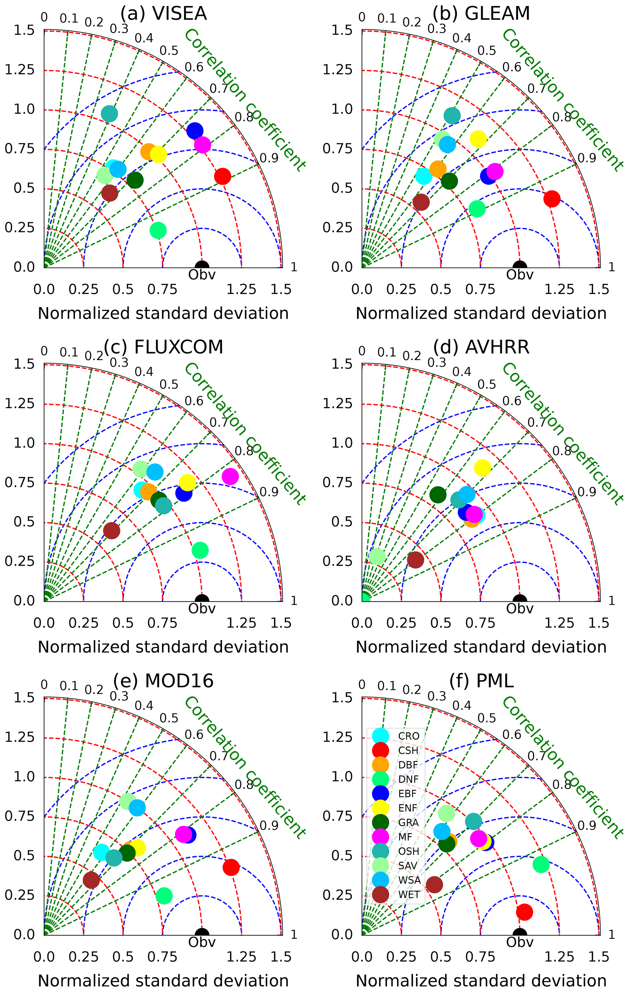
Figure 7Taylor diagrams comparing monthly measurements of (a) VISEA, GLEAM (b), FLUXCOM (c), AVHRR (d), MOD16 (e), and PML (f) with 150 flux towers (labeled “Obv”) in different IGBP land cover types. The diagrams display the normalized standard deviation (represented by red circles), the correlation coefficient (shown as green lines), and the centered root mean square (depicted as blue circles).
Table 3Statistical variables of six ET products – CC (correlation coefficient), ratio (the ratio of the standard deviations of simulated ET and flux tower measurements), bias, RMSE, RMSEu, RMSEs, and NSE.
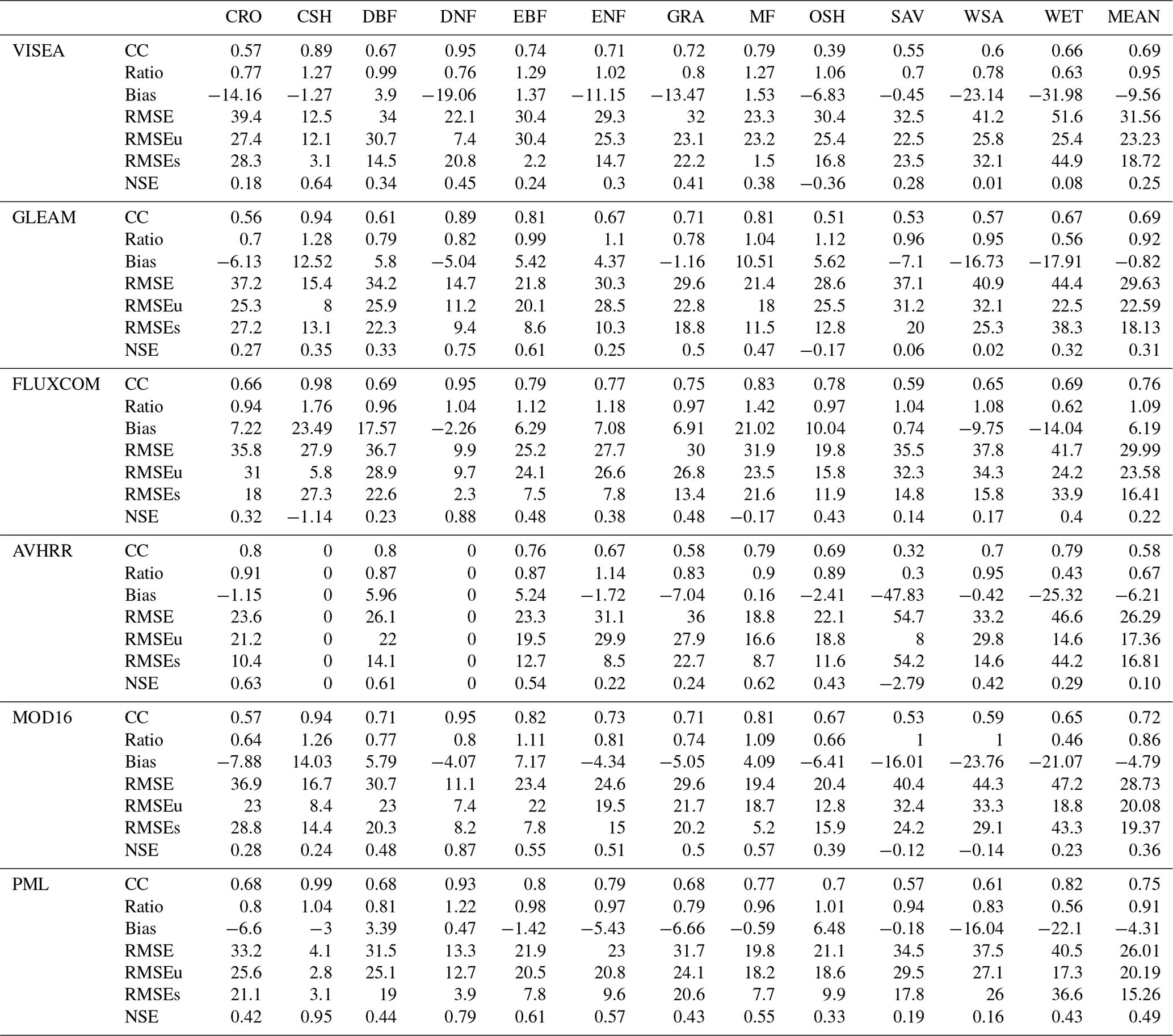
VISEA, with a mean CC of 0.69, indicates moderate correlation across vegetation types but suffers from significant biases, notably in WET, with a mean bias of −9.56 mm per month. It also has the highest mean RMSE of 31.6 mm per month and a mean NSE of 0.25. MOD16 demonstrates a slightly better correlation, with a mean CC of 0.72, and presents less variation in bias, resulting in a marginally lower mean RMSE of 28.7 mm per month and a higher mean NSE of 0.36. AVHRR matches VISEA with a mean CC at 0.69 but exhibits extreme biases, particularly in SAV, and achieves a comparable mean RMSE of 26.3 mm per month. However, its mean NSE of 0.10 is the lowest of the six products, suggesting that its predictions are less reliable.
On the other hand, GLEAM, FLUXCOM, and PML show better agreement. GLEAM has a high mean CC of 0.69 with the lowest bias of −0.82 mm per month, indicating consistent performance with a mean RMSE of 29.6 mm per month and a mean NSE of 0.31. FLUXCOM exhibits a higher mean CC of 0.76, suggesting better overall correlation, but with a higher mean bias of 6.2 mm per month it hints at a tendency towards overestimation. The mean RMSE is 30.0 mm per month, with a mean NSE of 0.22. PML outperforms the others, with the highest mean CC of 0.75 and the highest mean NSE of 0.49, indicating the strongest predictive accuracy. It also has the lowest mean RMSE of 26.0 mm per month.
Figure 8 illustrates the spatial distribution of the multiyear average (panels a–g), the zonal mean (panel h), and the interannual variation (panel i) of (panel a) GPCC (2001–2019), (panel b) VISEA (2001–2020), (panel c) GLEAM (2001–2020), (panel d) FLUXCOM (2001–2016), (panel e) AVHRR (2001–2006), (panel f) MOD16 (2001–2014), and (panel g) PML (2003–2018).
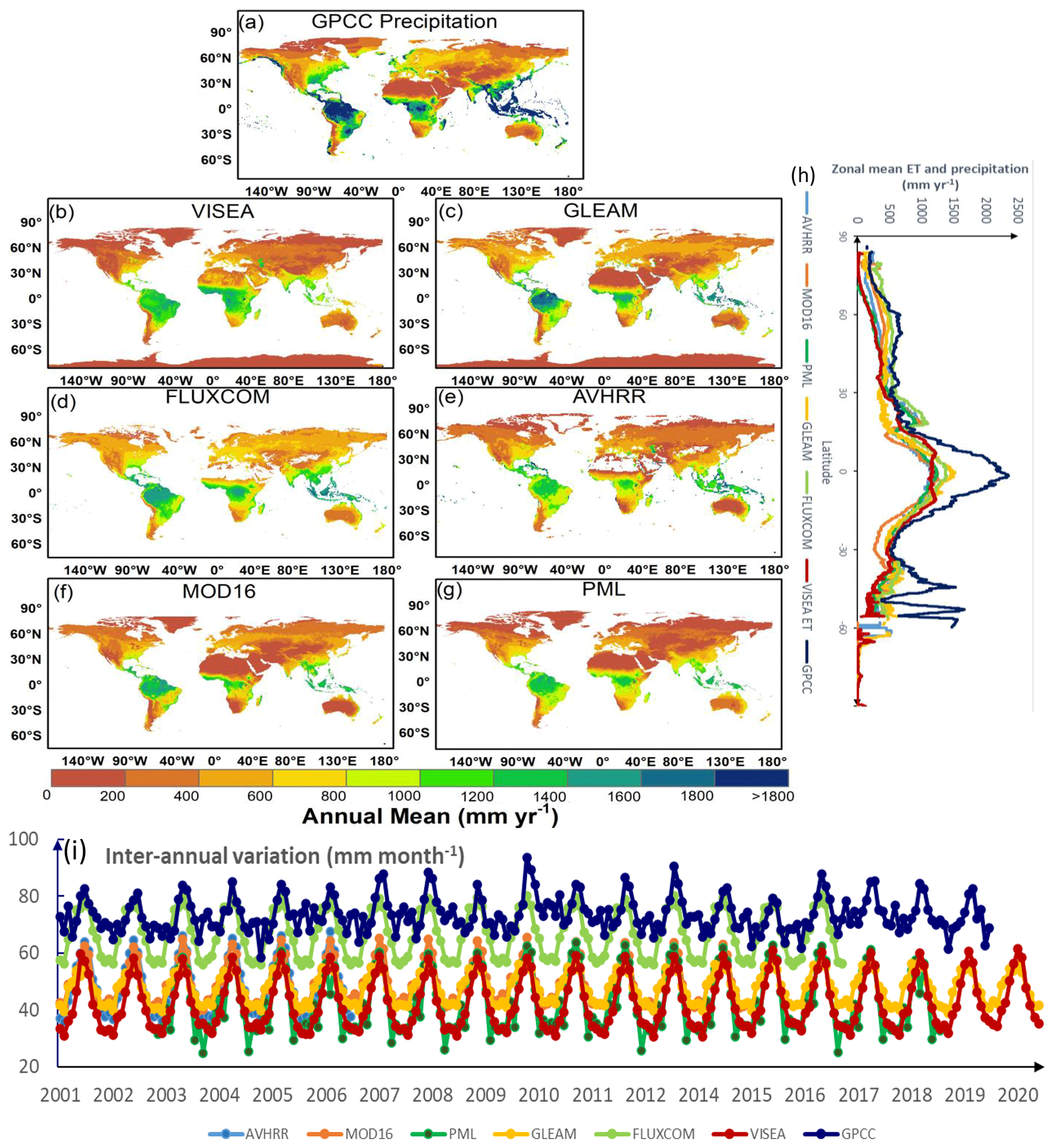
Figure 8The spatial distribution of the multiyear average (a–g), the zonal mean (h), and the interannual variation (i) of (a) GPCC precipitation (2001–2019), (b) VISEA (2001–2020), (c) GLEAM (2001–2020), (d) FLUXCOM (2001–2016), (e) AVHRR (2001–2006), (f) MOD16 (2001–2014), and (g) PML (2003–2018) ET data.
The VISEA ET product demonstrates consistent spatial distribution patterns among the six ET products across various years in terms of annual means (panels a–g) and latitudinal zonal means (panel h). These patterns closely align with the precipitation distribution data from GPCC. Furthermore, VISEA ET exhibits similar spatial distributions compared to other ET products, particularly in the extremes of the distribution below the 5th percentile and above the 95th percentile (Figs. S6 and S7 in the Supplement). The highest ET values, approximately 1500 mm yr−1, are predominantly in equatorial low-latitude regions with correspondingly high precipitation levels of approximately 2500 mm yr−1. These regions include South America (Amazon basin), central Africa (Congo basin), and Southeast Asia (encompassing Indonesia, Malaysia, parts of Thailand, and the Philippines), which have tropical rainforest climates. Remote sensing data support the ET estimates and align with findings from previous studies, such as Chen et al. (2021) and Zhang et al. (2019), who reported that the multiyear average annual ET is nearly 1500 and the precipitation is approximately 2500 mm yr−1. Also, Panagos et al. (2017) report similar multiyear average annual ET and precipitation rates.
In this analysis, barren (BAR) landscapes such as the Saharan, Arabian, Gobi, and Kalahari deserts; large areas of Australia; and snow and ice (SI) regions including significant parts of Canada, Russia, and the Qinghai–Tibet Plateau in China are characterized by notably low ET. These regions typically experience less than 400 mm yr−1 of annual ET, in parallel with minimal yearly precipitation ranging from 200 to 400 mm yr−1, according to GPCC data. Comparative ET rates for other land cover types generally range from 400 to 1400 mm yr−1, closely following the GPCC precipitation amounts from 600 to 1600 mm yr−1.
In regions experiencing moisture-limited ET, the scarcity of available water is the primary constraint. Conversely, in areas where sufficient water is available, ET is energy-limited, and factors such as cloud cover or shading restrict the absorption of solar radiation, affecting the evapotranspiration rate. Figure 8i illustrates interannual monthly variations over the past 2 decades. It shows how VISEA and other satellite-based ET products, alongside GPCC precipitation data, capture the rhythmic patterns of ET. These data reveal distinctive seasonal fluctuations and highlight the significant interannual climate variability. Of these products, FLUXCOM consistently shows ET values of 10–20 mm per month higher than those of other ET products. GLEAM and MOD16 exhibit similar ET estimations closely mirroring each other, as do PML and VISEA. Notably, after 2007, both GLEAM and MOD16 reported higher ET estimations than PML and VISEA in November, December, January, and February. For the same months, PML consistently records lower ET estimations than VISEA.
Analysis across the datasets reveals how ET estimates respond to extreme climate events, providing insights into the variability and resilience of these models. For instance, during the 2011–2012 drought in the Horn of Africa – one of the most severe droughts in recent decades – both ET estimations and GPCC precipitation data showed significant decreases. Similarly, the prolonged California drought from 2012 to 2016 also saw a considerable decrease in ET values, aligning with the reduced precipitation levels captured by GPCC.
Regarding the interannual monthly variations, panel (i) shows the fluctuations in ET across different years for the analyzed ET products and precipitation data. The graph reveals a rhythmic pattern of ET across the years. VISEA and other ET products showed distinctive peaks and troughs corresponding to seasonal changes and interannual climate variability. The ET products' data align closely with the precipitation patterns reported by GPCC, highlighting the interconnectedness between ET and precipitation as climatic variables. Notably, FLUXCOM consistently presents higher ET estimations than the other products. GLEAM's ET estimations are also slightly higher during the winter, indicating a trend of systematic overestimation in these products relative to the others in the dataset.
Figure 9 presents the daily ET from VISEA and GLEAM, alongside precipitation data from GPCC across the Yangtze River basin, from 26 August to 2 September 2022. During this period, a significant drought was observed in the region, which began in July and showed signs of abating by late August and early September, according to Zhang et al. (2023). VISEA ET illustrates the evolving drought conditions, with notably low ET levels (below 1 mm d−1) across the basin from 26 to 28 August, as shown in panels (a–c). A marked increase in precipitation on 29 August evident in panels (s) and (u) correlates with an uptick in ET values (surpassing 1 mm d−1) throughout the basin as visualized in panels (d–f). Although GLEAM generally captures the fluctuations in ET – both decreases and increases – during this period, it consistently reports much higher ET values than VISEA. The panel (y) graph in Fig. 9 shows the precipitation and ET calculated using VISAE and GLEAM after 11 mm rainfall on 29 August. The VISEA ET increased and decreased, which is expected because ET and soil moisture are positively correlated. GLEAM does not follow the expected pattern shown in panel (y). This comprehensive analysis highlights the interdependence of precipitation and ET and underscores the importance of considering soil moisture dynamics to fully understand the hydrological processes in the Yangtze River basin during extreme weather events.
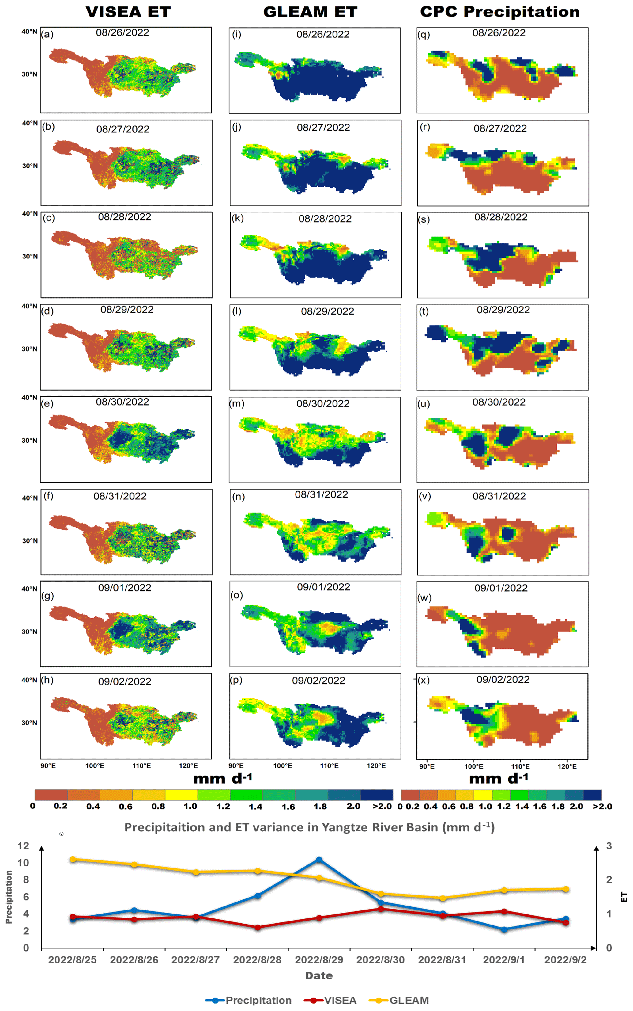
Figure 9Daily ET from VISEA (a–h), GLEAM (i–p), and CPC precipitation (q–x) distributions from 26 August to 2 September 2022, alongside daily mean ET and precipitation variances in the Yangtze River basin (y) during the same period.
Beyond precipitation, soil moisture is a critical regulator of ET, particularly during droughts and their recovery phases. Acting as a buffer, soil moisture tempers ET rates during dry periods and amplifies them after rainfall, as noted in late August. This buffering capacity results in a delay between precipitation events and subsequent ET changes, which is key to understanding drought recovery dynamics. VISEA's data accurately reflect these variations in precipitation, demonstrating their effectiveness in tracking daily ET fluctuations and their reliability for near-real-time monitoring of ET during hydrological extremes.
While global ET products (GLEAM, FLUXCOM, AVHRR, MOD16, and PML ET) require at least 2 weeks to generate global actual ET estimation, we developed VISEA, a satellite-based algorithm which is capable of generating near-real-time evapotranspiration at a daily time step with a resolution of 0.05°. To assess its accuracy, we compared the calculated ET with data from 149 flux towers around the world in various land use types.
Scale mismatch is a problem for many satellite-based ET products. The footprints of these flux towers typically range from 100 to 200 m, while the VISEA model outputs gridded cells at a resolution of 0.05°×0.05° (nearly 25 km2). This discrepancy introduces errors, especially since flux towers require a uniform fetch, which may not represent the larger gridded cell (Sun et al., 2023). To enhance the validity of our assessments, we assessed monthly values and spatial patterns of our ET measurements with five other satellite-based ET products, i.e., MOD16, AVHRR, GLEAM, FLUXCOM, and PML (Figs. 7 and 8).
The VISEA model uses gridded ERA5-Land shortwave downward radiation as its energy input. Utilizing this input, along with MODIS land surface products, VISEA calculates gridded daily air temperature and net radiation. These two important intermediate variables are essential for estimating daily ET. The calculated ET generally matches local measurements and other model-calculated values well, but we found significant biases (Figs. 6 and 7). These biases largely arise from inaccuracies in the input ERA5-Land shortwave radiation (Fig. 3), improper application of the VI–Ts method (Fig. 4), and uncertainties in daily net radiation (Fig. 5). Next, we look further into the causes of the biases.
Incoming shortwave radiation from ERA5-Land is employed to derive the available energy for vegetation coverage and bare soil (Eqs. 15 and 16), which are the main parameters for calculating daily ET (Eq. 17), while ERA5-Land is widely utilized as a reanalysis dataset, offering near-real-time land variables by integrating model data with global observations based on physical laws. However, the accuracy of shortwave radiation from ERA5-Land seems compromised in savannas (Fig. 3) due to the challenges associated with simulating radiation transmission under land use changes and aerosol pollution from natural or anthropogenic sources (Babar et al., 2019; Martens et al., 2020).
Air temperature is an important parameter in determining the daily evaporation fraction of bare soil (Appendix B), canopy surface resistance, aerodynamic resistance of the bare soil (Appendix C), atmospheric emissivity (Appendix D), and available energy for vegetation coverage and bare soil. Since air temperature is not measured directly by satellites, many other ET products use ground observations, land models, or reanalysis data. In contrast, VISEA derives the air temperature from the negative linear relationship between the VI and Ts using the VI–Ts method (Sect. 2.1.3). It gives very good results in the grassland, open shrubland, and woody savanna land cover types, as shown in Fig. 4. As previously explained, the VI–Ts method relies on the negative linear correlation between the VI and Ts within a 5×5 grid window. Therefore, the variance of VI values across these grid cells and the strength of their negative correlation are crucial for accurately calculating air temperature (Nishida et al., 2003). However, the VI–Ts method is less effective in regions like dense forests, bare landscapes, and deserts, where the vegetation index and temperature data vary little across the 5×5 grid window. Also, in regions with freezing temperatures, the VI–TS method does not perform well because warmer temperature is related to increased vegetation, which is the opposite of warmer areas, where there is a positive correlation between the vegetation index and surface temperature (Cui et al., 2021).
Other bias sources of the VISEA model are the uncertainties in daily net radiation, notably originating from input downward shortwave radiation from ERA5-Land- (Fig. 2) and VI–Ts-estimated air temperatures (Fig. 4). The energy budget equation (Eq. 14) and these two figures indicate that net radiation shows more uncertainties than shortwave radiation and air temperature. At the same time, assuming a linear relationship between cloud coverage (Eqs. 15 and 16) and calculating downward longwave radiation (Eqs. 17 and 18) may be an oversimplification that could introduce uncertainties. Since available energy for ET depends on net radiation (Eq. 14), addressing these uncertainties is crucial for enhancing overall model accuracy (Huang et al., 2023). Future refinements will contribute to a more precise daily net radiation estimation in the VISEA model.
The VISEA model calculates ET primarily based on vegetation coverage, utilizing it as an indirect constraint to estimate evapotranspiration. However, this model does not directly incorporate variables related to water availability, which is a critical factor in ET processes. In tropical regions, where solar radiation is abundant (available energy), the model tends to overestimate ET due to its emphasis on vegetation coverage without adequately accounting for the actual water available for evapotranspiration. This methodology, while effectively capturing the effect of vegetation on ET under varied conditions, can lead to overestimations in areas where energy availability significantly exceeds water availability, which is typical of many tropical regions. Our analysis and subsequent discussion aim to highlight this characteristic of the VISEA model, acknowledging its implications for ET estimations in such energy-rich, water-variable environments.
While the VISEA model provides ET globally, its best ET is between 60° N and 90° S, as evidenced by an NSE of 0.4 and a correlation coefficient (R) of 0.9 in Fig. 6. The VISEA model tends to underestimate ET in colder regions within the 60° N to 90° S latitude range, such as the western territories of Canada. This underestimation is primarily due to the model's inability to incorporate evaporation from frozen surfaces into its ET calculations. These discrepancies arise from several factors: inaccuracies in the ERA5-Land shortwave radiation data (illustrated in Fig. 3), the misapplication of the VI–Ts method (explained in Fig. 4), and the uncertainties in daily net radiation (depicted in Fig. 5). Designed to amalgamate bare soil and full vegetation coverage, as shown in Eq. (1), the VISEA model encounters difficulties in accurately estimating ET at higher latitudes, especially under conditions of reduced solar radiation. These challenges are predominantly linked to the uncertainties associated with ERA5-Land shortwave radiation data and are further compounded by increased cloudiness levels in these regions, as highlighted by Babar et al. (2019). Such uncertainties substantially impact the model's performance at higher latitudes, affecting its reliability under these conditions. Nevertheless, VISEA's ET estimates compare favorably with other ET data products in cold regions above 60° N, as indicated by the latitudinal zonal mean comparison in Fig. 8.
The accuracy of the VISEA model could be enhanced by incorporating additional satellite and climate data with higher resolution and improved accuracy. Moreover, the delay in providing ET data could be reduced to 3 d or less by integrating real-time updated satellite and climate data. We propose developing alternative methods for estimating air temperature and net radiation to enhance accuracy. Additionally, incorporating variables such as soil moisture and water availability into the model could further refine its precision. These improvements provide a roadmap for future research, aiming to significantly enhance satellite-based near-real-time ET modeling.
The VISEA ET data can be obtained from https://doi.org/10.11888/Terre.tpdc.300782 (Huang, 2023a). We are committed to continuously updating this dataset, ensuring that the latest ET data will be made available consistently and promptly.
6.1 Input data
MOD11C1 can be obtained at https://e4ftl01.cr.usgs.gov/MOLT/MOD11C1.061/ (USGS, 2023a). MOD09CMG can be obtained at https://e4ftl01.cr.usgs.gov/MOLT/MOD09CMG.061/ (USGS, 2023b). MCD43C3 can be obtained at https://e4ftl01.cr.usgs.gov/MOTA/MCD43C3.061/ (USGS, 2023c). MOD13C1 can be obtained at https://e4ftl01.cr.usgs.gov/MOLT/MOD13C1.061/ (USGS, 2023d). MCD12C1 can be obtained at https://e4ftl01.cr.usgs.gov/MOLT/MOD21C1.061/ (USGS, 2023e). ERA5-Land shortwave radiation data can be obtained at https://doi.org/10.24381/cds.e2161bac (Muñoz Sabater, 2019).
6.2 Evaluation data
FLUXNET2015 flux tower data (FLUXNET2015: CC-BY-4.0 33) can be obtained at https://fluxnet.org/data/download-data/ (last access: 12 May 2023). The GLEAM 3.8a ET dataset was obtained from https://www.gleam.eu/#downloads (last access: 12 May 2023) (an email is required to receive a password for the Secure File Transfer Protocol (SFTP). The FLUXCOM ET dataset is freely available (CC-BY-4.0 License) from the https://www.fluxcom.org/EF-Download/ (last access: 12 May 2023) data portal (an email is required to receive a password for the File Transfer Protocol (FTP). The MOD16 ET with a resolution of 0.05° was freely downloaded from http://files.ntsg.umt.edu/data/NTSG_Products/MOD16/MOD16A2_MONTHLY.MERRA_GMAO_1kmALB/Previous/ (Mu et al., 2011b). Additionally, the AVHRR ET dataset with 1° was sourced from http://files.ntsg.umt.edu/data/ET_global_monthly/Global_1DegResolution/ASCIIFormat/ (Zhang and Kimball, 2010). Lastly, the PML ET dataset was obtained from https://data.tpdc.ac.cn/zh-hans/data/48c16a8d-d307-4973-abab-972e9449627c (Zhang et al., 2020).
The precipitation from the GPCC data was obtained at https://doi.org/10.24381/cds.11dedf0c (Copernicus Climate Change Service, 2021). The precipitation from GPC was obtained at https://downloads.psl.noaa.gov/Datasets/cpc_global_precip/precip.2022.nc (NOAA, 2022).
Other data that support the analysis and conclusions of this work are available at https://doi.org/10.6084/m9.figshare.24669306.v1 (Huang, 2023b).
Python code to synthesize the results and to generate the figures from VISEA results and codes for the global ET products can be obtained through the public repository at https://doi.org/10.6084/m9.figshare.24647721.v1 (Huang, 2023c). The VISEA code to calculate daily ET is written in C and can be executed on Windows 10 using an Intel(R) Core (TM) i7-8565U CPU @ 1.80 GHz, 1.99 GHz, 16.0 GB RAM with Visual Studio 2019 or compatible platforms. Additionally, it can be run on high-performance-computing servers equipped with an Intel(R) Xeon(R) CPU E5-2680 in a CentOS environment. The system is scalable, supporting configurations ranging from 20 nodes and 656 CPUs down to fewer nodes and CPUs as required.
Several satellite-based ET products have been developed, but few estimate near-real-time global terrestrial ET. We have developed VISEA ET, which only uses satellite-based input data and can provide near-real-time global daily terrestrial ET estimates at a 0.05° spatial resolution. The accuracy of VISEA ET estimates is comparable to existing ET products sooner than existing products. Our evaluations show that VISEA aligns well with measurements from 149 globally distributed tower flux sites on daily and monthly scales. In addition, VISEA captures spatial patterns of evapotranspiration, aligning with GPCC precipitation data across diverse geographical regions, in particular highlighting elevated values in tropical rainforest regions and lower values in arid and semiarid zones. ET estimates are slightly too high in the Sahara and slightly too low in western Canada. Specifically, daily net radiation and ET estimations of VISEA in savanna and frozen surfaces need improvements. We plan to address these issues in future developments. The near-real-time global daily terrestrial ET estimates provided by VISEA are valuable for meteorology and hydrology applications, especially for coordinating relief efforts during droughts.
where the NDVI can be calculated as
where NDVImin is the NDVI of the bare soil without plants and NDVImax is the NDVI of the full vegetation cover. Rnir is the near-infrared reflectance and Rred is the red reflectance. The daily reflectances Rnir and Rred were measured by MODIS MOD09CMG reflectance data (Fig. 1). Based on Tang et al. (2009), we set NDVImin to 0.22 and NDVImax to 0.83. Missing observations for the daily MOD09CMG-calculated NDVI data were filled with the 16 d averaged NDVI values in the MOD13Q1 data product (Fig. 1).
is the value of the decoupling factor, Ω, for wet surfaces. According to Pereira (2004), Ω and Ω∗ can be expressed as
where rc is the surface resistance (s m−1) and ra is the aerodynamic resistance (s m−1), which are the calculation details of instantaneous and daily rc and ra for vegetation and soil. r∗ is the critical surface resistance when the actual evapotranspiration equals the potential evaporation (called the equilibrium evapotranspiration, s m−1). ρ is the air density (kg m−3). Cp is the specific heat of the air (). VPD is the vapor pressure deficit of the air (Pa). Δ is the slope of the saturated vapor pressure (Pa K−1).
The canopy surface resistance of the vegetation, denoted as rc veg (s m−1) and determined using the relationship established by Jarvis et al. (1976), is equivalent to
The minimum resistance rcMIN (s m−1) is defined as 33 s m−1 for cropland and 50 s m−1 for forest as determined by Tang et al. (2009). The canopy resistance related to diffusion through the cuticle layer of leaves rcuticle and set to 100 000 s m−1 in the Biome-Biosphere Model of the Carbon, Nitrogen, and Water Cycles (Biome-BGC) is from White et al. (2000). The relationships involving air temperature Ta, f1(Ta), and photosynthetically active radiation (PAR), f2(PAR), are expressed by the functions provided in Jarvis et al. (1976):
The minimum, optimal, and maximum temperatures for stomatal activity are denoted as Tn, To, and Tx, respectively. As per Tang et al. (2009), Tn is set to 275.85 K, To to 304.25 K, and Tx to 318.45 K. The expression for the function f2(PAR) is provided below:
where the PAR per unit area and time () is calculated using incoming solar radiation multiplied by 2.05 (White et al., 2000). A is a parameter related to photon absorption efficiency at low light intensity, which was set to 152 . Nishida et al. (2003) found that, in Eq. (D1), the following functions can be omitted without great loss of accuracy: the functions depend on vapor pressure deficit f3(VPD), leaf water potential f4(φ), and carbon dioxide vapor pressure f5(CO2).
The PAR per unit area and time () is computed by multiplying incoming solar radiation by 2.05, as outlined by White et al. (2000). The parameter A, associated with photon absorption efficiency at low light intensity, is set to 152 . Nishida et al. (2003) observed that, in Eq. (D1), the functions tied to vapor pressure deficit f3(VPD), leaf water potential f4(φ), and carbon dioxide vapor pressure f5(CO2) can be omitted without significant loss of accuracy. Tang et al. (2009) employed this canopy resistance approach to estimate ET at 500 m resolution in the Kalam River basin. The evaluation of their results indicated that the simplification of these calculations did not significantly impact the final accuracy of ET estimates. Additionally, Huang et al. (2017) evaluated this method for 0.05° ET assessments across China. In this study, we follow the methodologies originally developed by Tang et al. (2009) and Nishida et al. (2003), with the goal of enhancing the VISEA model to accurately estimate the daily-scale evaporation fraction and net radiation. These efforts build on earlier work by Huang et al. (2017, 2021, 2023) that introduced VPD and leaf water potential in calculating canopy resistance. However, comparative analyses between VISEA and other models such as PML and MOD16 – particularly PML, which integrates VPD as a limiting factor in estimating gross primary production (GPP) and ET – show that VISEA maintains accuracy without significant biases. It is important to note that none of the ET models in our comparison directly incorporates leaf water potential into their canopy resistance calculations. We are committed to addressing these gaps in our future studies.
The aerodynamic resistance of the canopy, denoted as ra veg (s m−1), is computed for forest cover, grassland, and cropland using the empirical formulae presented by Nishida et al. (2003) for both instantaneous and daily values:
The wind speed at a height of 50 m above the canopy (U50 m) is used to determine the aerodynamic resistance for grassland and cropland, as follows:
where U1 m is the wind speed 1 m above the canopy (m s−1). The wind speed as a function of the height z, U(z), can be calculated using the logarithm profile of wind. A recent study found that the velocity log law does not apply to a stratified atmospheric boundary layer (Cheng et al., 2011). Thus, Eqs. (D4) and (D5) are valid under neutral boundary layer conditions. Since ra veg is calculated differently for forests (Eq. D4) and grasslands or croplands (Eq. D5), we used the land cover classes from the yearly IGBP MCD12C1 to identify the land cover and choice of the different equation of ra veg. U50 m and U1 m were calculated using the logarithm profile of wind:
where Ushear is the shear velocity (m s−1), z is the height (m), and d is the surface displacement (m). z0 is the roughness length, where we followed Nishida et al. (2003), set to 0.005 m for bare soil and 0.01 m for grassland. k is the von Kármán constant and is set to 0.4 following Nishida (2003). The shear velocity Ushear was calculated as
where U1 m soil is the wind speed of bare soil at 1 m height (m s−1). This was calculated as
The VI–Ts diagram (Nishida et al., 2003) can be utilized to compute the instantaneous air temperature. This is achieved by utilizing MODIS instantaneous surface temperature and emissivity data (MOD11C1) and the daily calculated NDVI as input parameters.
The aerodynamic resistance of the bare soil, denoted as ra soil (s m−1), was determined by Nishida et al. (2003). This calculation assumes that the maximum surface temperature of bare soil Tsoil max (K) occurs when the sum of the latent heat flux and sensible heat flux of the bare soil, referred to as the available energy of bare soil Qsoil (W m−2), is utilized as the sensible heat flux while the latent heat flux is set to 0:
ra soil is the aerodynamic resistance of the bare soil (s m−1), ρ is the air density (kg m−3), Cp is the specific heat of the air (), Ta is the air temperature (K), and Qsoil is the available energy of bare soil (W m−2).
To compute the canopy surface resistance of bare soil, denoted as rc soil (s m−1), we adhere to the methodologies outlined in the works of van de Griend and Owe (1994) and Mu et al. (2007):
The total aerodynamic resistance rtot (s m−1) is composed of the aerodynamic resistance over the bare soil ra soil (s m−1), with atmospheric pressure P set to 101 300 Pa.
As per Brutsaert (1975), the atmospheric emissivity for clear skies under standard humidity and temperature conditions is
where represents the daily water vapor pressure (kPa). To calculate , it is necessary to compute the slope of the saturated vapor (Δ) as
VPD is the vapor pressure deficit of the air (kPa), which is expressed as
The expression in parentheses denotes the independent variable, where e0(Ta) represents the saturation vapor pressure (kPa) at the air temperature Ta (°C), ea is the actual vapor pressure (kPa), and e0(Tdew) is the saturation vapor pressure (kPa) at the dew point temperature Tdew (°C). For forest, water surface, and cropland, Tdew is set to the minimum air temperature during the day. In arid regions such as bare soil and non-irrigated grassland, Tdew may be 2–3 °C lower than Tmin. Therefore, 2 °C is subtracted from Tmin in arid and semiarid areas to derive Tdew. While these simplifications might introduce a bias into the final calculated ET value, our initial results indicate that the effect is negligible.
The supplement related to this article is available online at: https://doi.org/10.5194/essd-16-3993-2024-supplement.
LH had the original idea and drafted the paper with help from YL. JMC, QT, TS, WC, and WS participated in the discussion and the many manuscript revisions.
The contact author has declared that none of the authors has any competing interests.
Publisher's note: Copernicus Publications remains neutral with regard to jurisdictional claims made in the text, published maps, institutional affiliations, or any other geographical representation in this paper. While Copernicus Publications makes every effort to include appropriate place names, the final responsibility lies with the authors.
We employed ChatGPT3.5 to enhance the quality of our English writing and grammar. We also acknowledge the helpful comments and suggestions from the reviewers and the editorial team at Earth System Science Data.
This research has been supported by the Ministry of Science and Technology of the People's Republic of China and the National Key Research and Development Program of China (grant no. 2017YFA0603703) and the National Natural Science Foundation of China (grant no. 42305029).
This paper was edited by Jiafu Mao and reviewed by Mingliang Liu, Ren Wang, Seungcheol Oh, and Aolin Jia.
Albergel, C., Balsamo, G., de Rosnay, P., Muñoz-Sabater, J., and Boussetta, S.: A bare ground evaporation revision in the ECMWF land-surface scheme: evaluation of its impact using ground soil moisture and satellite microwave data, Hydrol. Earth Syst. Sci., 16, 3607–3620, https://doi.org/10.5194/hess-16-3607-2012, 2012.
Anderson, M. C., Yang, Y., Xue, J., Knipper, K. R., Yang, Y., Gao, F., Hain, C. R., Kustas, W. P., Cawse-Nicholson, K., Hulley, G., Fisher, J. B., Alfieri, J. G., Meyers, T. P., Prueger, J., Baldocchi, D. D., and Rey-Sanchez, C.: Interoperability of ECOSTRESS and Landsat for mapping evapotranspiration time series at sub-field scales, Remote Sens. Environ., 252, 112189, https://doi.org/10.1016/j.rse.2020.112189, 2021.
Aschonitis, V., Touloumidis, D., ten Veldhuis, M.-C., and Coenders-Gerrits, M.: Correcting Thornthwaite potential evapotranspiration using a global grid of local coefficients to support temperature-based estimations of reference evapotranspiration and aridity indices, Earth Syst. Sci. Data, 14, 163–177, https://doi.org/10.5194/essd-14-163-2022, 2022.
Awada, H., Di Prima, S., Sirca, C., Giadrossich, F., Marras, S., Spano, D., and Pirastru, M.: A remote sensing and modeling integrated approach for constructing continuous time series of daily actual evapotranspiration, Agr. Water Manage., 260, 107320, https://doi.org/10.1016/j.agwat.2021.107320, 2022.
Babar, B., Graversen, R., and Boström, T.: Solar radiation estimation at high latitudes: Assessment of the CMSAF databases, ASR and ERA5, Sol. Energy, 182, 397–411, https://doi.org/10.1016/j.solener.2019.02.058, 2019.
Baldocchi, D., Falge, E., Gu, L., Olson, R., Hollinger, D., Running, S., Anthoni, P., Bernhofer, C., Davis, K., Evans, R., Fuentes, J., Goldstein, A., Katul, G., Law, B., Lee, X., Malhi, Y., Meyers, T., Munger, W., Oechel, W., Paw U, K. T., Pilegaard, K., Schmid, H. P., Valentini, R., Verma, S., Vesala, T., Wilson, K., and Wofsy, S.: FLUXNET: A new tool to study the temporal and spatial variability of ecosystem-scale carbon dioxide, water vapor, and energy flux densities, B. Am. Meteorol. Soc., 82, 2415–2434, https://doi.org/10.1175/1520-0477(2001)082<2415:FANTTS>2.3.CO;2, 2001.
Barrios, J. M., Ghilain, N., Arboleda, A., and Gellens-Meulenberghs, F.: Retrieving daily evapotranspiration from the combination of geostationary and polar-orbit satellite data, in: 2015 8th International Workshop on the Analysis of Multitemporal Remote Sensing Images (Multi-Temp), Annecy, France, 22–24 July 2015, 1–4, https://doi.org/10.1109/Multi-Temp.2015.7245797, 2015.
Becker, A., Finger, P., Meyer-Christoffer, A., Rudolf, B., Schamm, K., Schneider, U., and Ziese, M.: A description of the global land-surface precipitation data products of the Global Precipitation Climatology Centre with sample applications including centennial (trend) analysis from 1901–present, Earth Syst. Sci. Data, 5, 71–99, https://doi.org/10.5194/essd-5-71-2013, 2013.
Brutsaert, W.: On a derivable formula for long-wave radiation from clear skies, Water Resour. Res., 11, 742–744, https://doi.org/10.1029/WR011i005p00742, 1975.
Chang, K. and Zhang, Q.: Modeling of downward longwave radiation and radiative cooling potential in China, J. Renew. Sustain. Ener., 11, 066501, https://doi.org/10.1063/1.5117319, 2019.
Chen, X., Su, Z., Ma, Y., Trigo, I., and Gentine, P.: Remote Sensing of Global Daily Evapotranspiration based on a Surface Energy Balance Method and Reanalysis Data, J. Geophys. Res.-Atmos., 126, e2020JD032873, https://doi.org/10.1029/2020JD032873, 2021.
Cheng, L., Xu, Z., Wang, D., and Cai, X.: Assessing interannual variability of evapotranspiration at the catchment scale using satellite-based evapotranspiration data sets, Water Resour. Res., 47, , W09502, https://doi.org/10.1029/2011WR010636, 2011.
Copernicus Climate Change Service: Crop productivity and evapotranspiration indicators from 2000 to present derived from satellite observations, https://doi.org/10.24381/CDS.B2F6F9F6, 2020.
Copernicus Climate Change Service: Temperature and precipitation gridded data for global and regional domains derived from in-situ and satellite observations, Copernicus Climate Change Service (C3S) Climate Data Store (CDS) [data set], https://doi.org/10.24381/cds.11dedf0c, 2021.
Cui, Y., Jia, L., and Fan, W.: Estimation of actual evapotranspiration and its components in an irrigated area by integrating the Shuttleworth-Wallace and surface temperature-vegetation index schemes using the particle swarm optimization algorithm, Agr. Forest Meteorol., 307, 108488, https://doi.org/10.1016/j.agrformet.2021.108488, 2021.
De Bruin, H. A. R.: A Model for the Priestley-Taylor Parameter α, J. Appl. Meteorol. Clim., 22, 572–578, https://doi.org/10.1175/1520-0450(1983)022<0572:AMFTPT>2.0.CO;2, 1983.
FAO: Crop evapotranspiration – Guidelines for computing crop water requirements, edited by: Allen, G. R., Pereira, S. L., Raes, D., and Smith, M., FAO, Rome, ISBN 92-5-104219-5, 1998.
Fisher, J. B., Lee, B., Purdy, A. J., Halverson, G. H., Dohlen, M. B., Cawse-Nicholson, K., Wang, A., Anderson, R. G., Aragon, B., Arain, M. A., Baldocchi, D. D., Baker, J. M., Barral, H., Bernacchi, C. J., Bernhofer, C., Biraud, S. C., Bohrer, G., Brunsell, N., Cappelaere, B., Castro-Contreras, S., Chun, J., Conrad, B. J., Cremonese, E., Demarty, J., Desai, A. R., De Ligne, A., Foltýnová, L., Goulden, M. L., Griffis, T. J., Grünwald, T., Johnson, M. S., Kang, M., Kelbe, D., Kowalska, N., Lim, J.-H., Maïnassara, I., McCabe, M. F., Missik, J. E. C., Mohanty, B. P., Moore, C. E., Morillas, L., Morrison, R., Munger, J. W., Posse, G., Richardson, A. D., Russell, E. S., Ryu, Y., Sanchez-Azofeifa, A., Schmidt, M., Schwartz, E., Sharp, I., Šigut, L., Tang, Y., Hulley, G., Anderson, M., Hain, C., French, A., Wood, E., and Hook, S.: ECOSTRESS: NASA’s Next Generation Mission to Measure Evapotranspiration From the International Space Station, Water Resour. Res., 56, e2019WR026058, https://doi.org/10.1029/2019WR026058, 2020.
Fisher, J. B., Lee, B., Purdy, A. J., Halverson, G. H., Dohlen, M. B., Cawse-Nicholson, K., Wang, A., Anderson, R. G., Aragon, B., Arain, M. A., Baldocchi, D. D., Baker, J. M., Barral, H., Bernacchi, C. J., Bernhofer, C., Biraud, S. C., Bohrer, G., Brunsell, N., Cappelaere, B., Castro-Contreras, S., Chun, J., Conrad, B. J., Cremonese, E., Demarty, J., Desai, A. R., De Ligne, A., Foltýnová, L., Goulden, M. L., Griffis, T. J., Grünwald, T., Johnson, M. S., Kang, M., Kelbe, D., Kowalska, N., Lim, J.-H., Maïnassara, I., McCabe, M. F., Missik, J. E. C., Mohanty, B. P., Moore, C. E., Morillas, L., Morrison, R., Munger, J. W., Posse, G., Richardson, A. D., Russell, E. S., Ryu, Y., Sanchez-Azofeifa, A., Schmidt, M., Schwartz, E., Sharp, I., Šigut, L., Tang, Y., Hulley, G., Anderson, M., Hain, C., French, A., Wood, E., and Hook, S.: ECOSTRESS: NASA's Next Generation Mission to Measure Evapotranspiration From the International Space Station, Water Resour. Res., 56, e2019WR026058, https://doi.org/10.1029/2019WR026058, 2020.
Fritschen, L. J. and Gay, L. W.: Soil Heat Flux, in: Environmental Instrumentation, edited by: Fritschen, L. J. and Gay, L. W., Springer, New York, NY, 86–92, https://doi.org/10.1007/978-1-4612-6205-3_4, 1979.
Goforth, M. A., Gilchrist, G. W., and Sirianni, J. D.: Cloud effects on thermal downwelling sky radiance, in: Thermosense XXIV, edited by: McCarthy, D. M., Peacock, R. D., Proceedings of SPIE, vol. 4710, International Society for Optics and Photonics, Bellingham, WA, USA, 203–213, https://doi.org/10.1117/12.459570, 2002.
Han, C., Ma, Y., Wang, B., Zhong, L., Ma, W., Chen, X., and Su, Z.: Long-term variations in actual evapotranspiration over the Tibetan Plateau, Earth Syst. Sci. Data, 13, 3513–3524, https://doi.org/10.5194/essd-13-3513-2021, 2021.
He, S., Zhang, Y., Ma, N., Tian, J., Kong, D., and Liu, C.: A daily and 500 m coupled evapotranspiration and gross primary production product across China during 2000–2020, Earth Syst. Sci. Data, 14, 5463–5488, https://doi.org/10.5194/essd-14-5463-2022, 2022.
Huang, L.: Satellite-based Near-Real-Time Global Terrestrial Evapotranspiration Estimation Dataset, TPDC [data set], https://doi.org/10.11888/Terre.tpdc.300782, 2023a.
Huang, L.: Satellite-based Near-Real-Time Global Daily Terrestrial Evapotranspiration Estimates, Figshare [data set], https://doi.org/10.6084/m9.figshare.24669306.v1, 2023b.
Huang, L.: Satellite-based Near-Real-Time Global Daily Terrestrial Evapotranspiration Estimates, Figshare [software], https://doi.org/10.6084/m9.figshare.24647721.v1, 2023c.
Huang, L., Li, Z., Tang, Q., Zhang, X., Liu, X., and Cui, H.: Evaluation of satellite-based evapotranspiration estimates in China, J. Appl. Remote Sens., 11, 026019, https://doi.org/10.1117/1.JRS.11.026019, 2017.
Huang, L., Steenhuis, T. S., Luo, Y., Tang, Q., Tang, R., Zheng, J., Shi, W., and Qiao, C.: Revisiting Daily MODIS Evapotranspiration Algorithm Using Flux Tower Measurements in China, Earth and Space Science, 8, e2021EA001818, https://doi.org/10.1029/2021EA001818, 2021.
Huang, L., Luo, Y., Steenhuis, T., Tang, Q., Cheng, W., Shi, W., Xia, X., Zhao, D., and Liao, Z.: An Improved Satellite-Based Evapotranspiration Procedure for China, Earth and Space Science, 10, e2023EA002949, https://doi.org/10.1029/2023EA002949, 2023.
Idso, S. B., Aase, J. K., and Jackson, R. D.: Net radiation – soil heat flux relations as influenced by soil water content variations, Bound.-Lay. Meteorol., 9, 113–122, https://doi.org/10.1007/BF00232257, 1975.
Jaafar, H., Mourad, R., and Schull, M.: A global 30 m ET model (HSEB) using harmonized Landsat and Sentinel-2, MODIS and VIIRS: Comparison to ECOSTRESS ET and LST, Remote Sens. Environ., 274, 112995, https://doi.org/10.1016/j.rse.2022.112995, 2022.
Jarlan, L., Balsamo, G., Lafont, S., Beljaars, A., Calvet, J. C., and Mougin, E.: Analysis of leaf area index in the ECMWF land surface model and impact on latent heat and carbon fluxes: Application to West Africa, J. Geophys. Res.-Atmos., 113, D24117, https://doi.org/10.1029/2007JD009370, 2008.
Jarvis, P. G., Monteith, J. L., and Weatherley, P. E.: The interpretation of the variations in leaf water potential and stomatal conductance found in canopies in the field, Philos. T. Roy. Soc. B, 273, 593–610, https://doi.org/10.1098/rstb.1976.0035, 1976.
Jiang, H., Yang, Y., Bai, Y., and Wang, H.: Evaluation of the Total, Direct, and Diffuse Solar Radiations From the ERA5 Reanalysis Data in China, IEEE Geosci. Remote S., 17, 47–51, https://doi.org/10.1109/LGRS.2019.2916410, 2020.
Jung, M., Reichstein, M., and Bondeau, A.: Towards global empirical upscaling of FLUXNET eddy covariance observations: validation of a model tree ensemble approach using a biosphere model, Biogeosciences, 6, 2001–2013, https://doi.org/10.5194/bg-6-2001-2009, 2009.
Jung, M., Reichstein, M., Ciais, P., Seneviratne, S. I., Sheffield, J., Goulden, M. L., Bonan, G., Cescatti, A., Chen, J., de Jeu, R., Dolman, A. J., Eugster, W., Gerten, D., Gianelle, D., Gobron, N., Heinke, J., Kimball, J., Law, B. E., Montagnani, L., Mu, Q., Mueller, B., Oleson, K., Papale, D., Richardson, A. D., Roupsard, O., Running, S., Tomelleri, E., Viovy, N., Weber, U., Williams, C., Wood, E., Zaehle, S., and Zhang, K.: Recent decline in the global land evapotranspiration trend due to limited moisture supply, Nature, 467, 951–954, https://doi.org/10.1038/nature09396, 2010.
Jung, M., Koirala, S., Weber, U., Ichii, K., Gans, F., Camps-Valls, G., Papale, D., Schwalm, C., Tramontana, G., and Reichstein, M.: FLUXCOM Global Land Energy Fluxes, https://doi.org/10.17871/FLUXCOM_EnergyFluxes_v1, 2018.
Jung, M., Koirala, S., Weber, U., Ichii, K., Gans, F., Camps-Valls, G., Papale, D., Schwalm, C., Tramontana, G., and Reichstein, M.: The FLUXCOM ensemble of global land-atmosphere energy fluxes, Sci. Data, 6, 1–14, https://doi.org/10.1038/s41597-019-0076-8, 2019.
Liu, Z., Jiang, L., Shi, C., Zhang, T., Zhou, Z., Liao, J., Yao, S., Liu, J., Wang, M., Wang, H., Liang, X., Zhang, Z., Yao, Y., Zhu, T., Chen, Z., Xu, W., Cao, L., Jiang, H., and Hu, K.: CRA-40/Atmosphere – The First-Generation Chinese Atmospheric Reanalysis (1979–2018): System Description and Performance Evaluation, J. Meteorol. Res.-PRC, 37, 1–19, https://doi.org/10.1007/s13351-023-2086-x, 2023.
Martens, B., Miralles, D. G., Lievens, H., van der Schalie, R., de Jeu, R. A. M., Fernández-Prieto, D., Beck, H. E., Dorigo, W. A., and Verhoest, N. E. C.: GLEAM v3: satellite-based land evaporation and root-zone soil moisture, Geosci. Model Dev., 10, 1903–1925, https://doi.org/10.5194/gmd-10-1903-2017, 2017.
Martens, B., Schumacher, D. L., Wouters, H., Muñoz-Sabater, J., Verhoest, N. E. C., and Miralles, D. G.: Evaluating the land-surface energy partitioning in ERA5, Geosci. Model Dev., 13, 4159–4181, https://doi.org/10.5194/gmd-13-4159-2020, 2020.
Miller, M. J., Beljaars, A. C. M., and Palmer, T. N.: The Sensitivity of the ECMWF Model to the Parameterization of Evaporation from the Tropical Oceans, J. Climate, 5, 418–434, https://doi.org/10.1175/1520-0442(1992)005<0418:TSOTEM>2.0.CO;2, 1992.
Miralles, D. G., Holmes, T. R. H., De Jeu, R. A. M., Gash, J. H., Meesters, A. G. C. A., and Dolman, A. J.: Global land-surface evaporation estimated from satellite-based observations, Hydrol. Earth Syst. Sci., 15, 453–469, https://doi.org/10.5194/hess-15-453-2011, 2011.
Mu, Q., Heinsch, F. A., Zhao, M., and Running, S. W.: Development of a global evapotranspiration algorithm based on MODIS and global meteorology data, Remote Sens. Environ., 111, 519–536, https://doi.org/10.1016/j.rse.2007.04.015, 2007.
Mu, Q., Zhao, M., and Running, S. W.: Improvements to a MODIS global terrestrial evapotranspiration algorithm, Remote Sens. Environ., 115, 1781–1800, https://doi.org/10.1016/j.rse.2011.02.019, 2011a.
Mu, Q., Zhao, M., and Running, S. W: The MOD16 global evapotranspiration (ET)/latent heat flux (LE)/potential ET (PET)/potential LE (PLE) datasets, NASA [data set], http://files.ntsg.umt.edu/data/NTSG_Products/MOD16/MOD16A2_MONTHLY.MERRA_GMAO_1kmALB/Previous/ (last access: 12 May 2023), 2011b.
Muñoz Sabater, J.: ERA5-Land hourly data from 1950 to present, Copernicus Climate Change Service (C3S) Climate Data Store (CDS) [data set], https://doi.org/10.24381/cds.e2161bac, 2019.
National Oceanic and Atmospheric Administration (NOAA): Climate Prediction Center (CPC) Global Precipitation Data, NOAA [Data set], https://downloads.psl.noaa.gov/Datasets/cpc_global_precip/precip.2022.nc (last access: 12 May 2023), 2022.
Naud, C. M., Booth, J. F., and Genio, A. D. D.: Evaluation of ERA-Interim and MERRA Cloudiness in the Southern Ocean, J. Climate, 27, 2109–2124, https://doi.org/10.1175/JCLI-D-13-00432.1, 2014.
Nishida, K., Nemani, R. R., Running, S. W., and Glassy, J. M.: An operational remote sensing algorithm of land surface evaporation, J. Geophys. Res.-Atmos., 108, 4270, https://doi.org/10.1029/2002JD002062, 2003.
Norman, J. M., Kustas, W. P., and Humes, K. S.: Source approach for estimating soil and vegetation energy fluxes in observations of directional radiometric surface temperature, Agr. Forest Meteorol., 77, 263–293, https://doi.org/10.1016/0168-1923(95)02265-Y, 1995.
Panagos, P., Borrelli, P., Meusburger, K., Yu, B., Klik, A., Yang, J., Ni, J., Chattopadhyay, N., Sadeghi, S. H., Hazbavi, Z., Zabihi, M., Larionov, G., Krasnov, S., Gorobets, A., Levi, Y., Erpul, G., Birkel, C., and Ballabio, C.: Global rainfall erosivity assessment based on high-temporal resolution rainfall records, Sci. Rep.-UK, 7, 4175, https://doi.org/10.1038/s41598-017-04282-8, 2017.
Pastorello, G., Trotta, C., Canfora, E., et al.: The FLUXNET2015 dataset and the ONEFlux processing pipeline for eddy covariance data, Sci. Data, 7, 225, https://doi.org/10.1038/s41597-020-0534-3, 2020.
Pereira, A. R.: The Priestley–Taylor parameter and the decoupling factor for estimating reference evapotranspiration, Agr. Forest Meteorol., 125, 305–313, https://doi.org/10.1016/j.agrformet.2004.04.002, 2004.
Schneider, U., Becker, A., Finger, P., Meyer-Christoffer, A., Rudolf, B., and Ziese, M.: GPCC Full Data Reanalysis Version 6.0 at 2.5°: Monthly Land-Surface Precipitation from Rain-Gauges built on GTS-based and Historic Data, https://doi.org/10.5676/DWD_GPCC/FD_M_V7_250, 2011.
Schneider, U., Becker, A., Finger, P., Meyer-Christoffer, A., Ziese, M., and Rudolf, B.: GPCC's new land surface precipitation climatology based on quality-controlled in situ data and its role in quantifying the global water cycle, Theor. Appl. Climatol., 115, 15–40, https://doi.org/10.1007/s00704-013-0860-x, 2014.
Schneider, U., Finger, P., Meyer-Christoffer, A., Rustemeier, E., Ziese, M., and Becker, A.: Evaluating the Hydrological Cycle over Land Using the Newly-Corrected Precipitation Climatology from the Global Precipitation Climatology Centre (GPCC), Atmosphere, 8, 52, https://doi.org/10.3390/atmos8030052, 2017.
Su, B., Huang, J., Mondal, S. K., Zhai, J., Wang, Y., Wen, S., Gao, M., Lv, Y., Jiang, S., Jiang, T., and Li, A.: Insight from CMIP6 SSP-RCP scenarios for future drought characteristics in China, Atmos. Res., 250, 105375, https://doi.org/10.1016/j.atmosres.2020.105375, 2020.
Sun, S., Bi, Z., Xiao, J., Liu, Y., Sun, G., Ju, W., Liu, C., Mu, M., Li, J., Zhou, Y., Li, X., Liu, Y., and Chen, H.: A global 5 km monthly potential evapotranspiration dataset (1982–2015) estimated by the Shuttleworth–Wallace model, Earth Syst. Sci. Data, 15, 4849–4876, https://doi.org/10.5194/essd-15-4849-2023, 2023.
Tang, Q., Peterson, S., Cuenca, R. H., Hagimoto, Y., and Lettenmaier, D. P.: Satellite-based near-real-time estimation of irrigated crop water consumption, J. Geophys. Res.-Atmos., 114, D05114, https://doi.org/10.1029/2008JD010854, 2009.
Tang, R. and Li, Z.-L.: An improved constant evaporative fraction method for estimating daily evapotranspiration from remotely sensed instantaneous observations, Geophys. Res. Lett., 44, 2319–2326, https://doi.org/10.1002/2017GL072621, 2017.
Tang, R., Li, Z.-L., Sun, X., and Bi, Y.: Temporal upscaling of instantaneous evapotranspiration on clear-sky days using the constant reference evaporative fraction method with fixed or variable surface resistances at two cropland sites, J. Geophys. Res.-Atmos., 122, 784–801, https://doi.org/10.1002/2016JD025975, 2017.
Taylor, K. E.: Summarizing multiple aspects of model performance in a single diagram, J. Geophys. Res.-Atmos., 106, 7183–7192, https://doi.org/10.1029/2000JD900719, 2001.
US Geological Survey (USGS): MOD11C1 – MODIS/Terra Land Surface Temperature and Emissivity Daily L3 Global 1km Grid, Version 061, USGS [data set], https://e4ftl01.cr.usgs.gov/MOLT/MOD11C1.061/, last access: 12 May 2023a.
US Geological Survey (USGS): MOD09CMG – MODIS/Terra Surface Reflectance Daily L3 Global 500m Grid, Version 061, USGS [data set], https://e4ftl01.cr.usgs.gov/MOLT/MOD09CMG.061/, last access: 12 May 2023b.
US Geological Survey (USGS): MCD43C3 – MODIS/Terra+Aqua BRDF/Albedo Daily L3 Global 500m Grid, Version 061, USGS [data set], https://e4ftl01.cr.usgs.gov/MOTA/MCD43C3.061/, last access: 12 May 2023c.
US Geological Survey (USGS): MOD13C1 – MODIS/Terra Vegetation Indices 16-Day L3 Global 500m Grid, Version 061, USGS [data set], https://e4ftl01.cr.usgs.gov/MOLT/MOD13C1.061/, last access on 12 May 2023d.
US Geological Survey (USGS): MCD12C1 – MODIS/Terra+Aqua Land Cover Type Yearly L3 Global 500m Grid, Version 061, USGS [data set], https://e4ftl01.cr.usgs.gov/MOLT/MOD21C1.061/, last access: 12 May 2023e.
van de Griend, A. A. and Owe, M.: Bare soil surface resistance to evaporation by vapor diffusion under semiarid conditions, Water Resour. Res., 30, 181–188, https://doi.org/10.1029/93WR02747, 1994.
Wang, K. and Dickinson, R. E.: Global atmospheric downward longwave radiation at the surface from ground-based observations, satellite retrievals, and reanalyses, Rev. Geophys., 51, 150–185, https://doi.org/10.1002/rog.20009, 2013.
Wang, L., Liu, H., Chen, D., Zhang, P., Leavitt, S., Liu, Y., Fang, C., Sun, C., Cai, Q., Gui, Z., Liang, B., Shi, L., Liu, F., Zheng, Y., and Grießinger, J.: The 1820s Marks a Shift to Hotter-Drier Summers in Western Europe Since 1360, Geophys. Res. Lett., 49, e2022GL099692, https://doi.org/10.1029/2022GL099692, 2022.
Wang, R., Gentine, P., Yin, J., Chen, L., Chen, J., and Li, L.: Long-term relative decline in evapotranspiration with increasing runoff on fractional land surfaces, Hydrol. Earth Syst. Sci., 25, 3805–3818, https://doi.org/10.5194/hess-25-3805-2021, 2021.
Wang, Y., Zhao, X., Mamtimin, A., Sayit, H., Abulizi, S., Maturdi, A., Yang, F., Huo, W., Zhou, C., Yang, X., and Liu, X.: Evaluation of Reanalysis Datasets for Solar Radiation with In Situ Observations at a Location over the Gobi Region of Xinjiang, China, Remote Sens.-Basel, 13, 4191, https://doi.org/10.3390/rs13214191, 2021.
White, M. A., Thornton, P. E., Running, S. W., and Nemani, R. R.: Parameterization and Sensitivity Analysis of the BIOME–BGC Terrestrial Ecosystem Model: Net Primary Production Controls, Earth Interact., 4, 1–85, https://doi.org/10.1175/1087-3562(2000)004<0003:PASAOT>2.0.CO;2, 2000.
Willmott, C. J.: On the Validation of Models, Phys. Geogr., 2, 184–194, https://doi.org/10.1080/02723646.1981.10642213, 1981.
Yang, D., Chen, H., and Lei, H.: Analysis of the Diurnal Pattern of Evaporative Fraction and Its Controlling Factors over Croplands in the Northern China, J. Integr. Agr., 12, 1316–1329, https://doi.org/10.1016/S2095-3119(13)60540-7, 2013.
Yang, R. and Friedl, M. A.: Modeling the effects of three-dimensional vegetation structure on surface radiation and energy balance in boreal forests, J. Geophys. Res.-Atmos., 108, D16S90, https://doi.org/10.1029/2002JD003109, 2003.
Zhang, C., Long, D., Zhang, Y., Anderson, M. C., Kustas, W. P., and Yang, Y.: A decadal (2008–2017) daily evapotranspiration data set of 1 km spatial resolution and spatial completeness across the North China Plain using TSEB and data fusion, Remote Sens. Environ., 262, 112519, https://doi.org/10.1016/j.rse.2021.112519, 2021.
Zhang, K. and Kimball, J.: A continuous satellite-derived global record of land surface evapotranspiration from 1983 to 2006, University of Montana [data set], http://files.ntsg.umt.edu/data/ET_global_monthly/Global_1DegResolution/ASCIIFormat/ (last access: 12 May 2023), 2010.
Zhang, K., Kimball, J. S., Mu, Q., Jones, L. A., Goetz, S. J., and Running, S. W.: Satellite based analysis of northern ET trends and associated changes in the regional water balance from 1983 to 2005, J. Hydrol., 379, 92–110, https://doi.org/10.1016/j.jhydrol.2009.09.047, 2009.
Zhang, K., Kimball, J. S., Nemani, R. R., and Running, S. W.: A continuous satellite-derived global record of land surface evapotranspiration from 1983 to 2006, Water Resour. Res., 46, W09522, https://doi.org/10.1029/2009WR008800, 2010.
Zhang, X., Huang, A., Dai, Y., Li, W., Gu, C., Yuan, H., Wei, N., Zhang, Y., Qiu, B., and Cai, S.: Influences of 3D Sub-Grid Terrain Radiative Effect on the Performance of CoLM Over Heihe River Basin, Tibetan Plateau, J. Adv. Model. Earth Sy., 14, e2021MS002654, https://doi.org/10.1029/2021MS002654, 2022.
Zhang, Y.: PML_V2 global evapotranspiration and gross primary production (2002.07-2019.08), National Tibetan Plateau/Third Pole Environment Data Center [data set], https://data.tpdc.ac.cn/zh-hans/data/48c16a8d-d307-4973-abab-972e9449627c (last access: 12 May 2023), 2020.
Zhang, Y., Kong, D., Gan, R., Chiew, F. H. S., McVicar, T. R., Zhang, Q., and Yang, Y.: Coupled estimation of 500 m and 8 d resolution global evapotranspiration and gross primary production in 2002–2017, Remote Sens. Environ., 222, 165–182, https://doi.org/10.1016/j.rse.2018.12.031, 2019.
Zhang, Y., Li, C., Chiew, F. H. S., Post, D. A., Zhang, X., Ma, N., Tian, J., Kong, D., Leung, L. R., Yu, Q., Shi, J., and Liu, C.: Southern Hemisphere dominates recent decline in global water availability, Science, 382, 579–584, https://doi.org/10.1126/science.adh0716, 2023.
Zhao, B., Zhang, B., Shi, C., Liu, J., and Jiang, L.: Comparison of the Global Energy Cycle between Chinese Reanalysis Interim and ECMWF Reanalysis, J. Meteorol. Res.-PRC, 33, 563–575, https://doi.org/10.1007/s13351-019-8129-7, 2019.
- Abstract
- Introduction
- Methods
- Data
- Results
- Discussion
- Data availability
- Code availability
- Conclusion
- Appendix A: Determining the vegetation fraction calculation
- Appendix B: Determining the decoupling factor
- Appendix C: Determining the resistances of the vegetation canopy and bare soil surface
- Appendix D: The calculation of atmospheric emissivity for clear skies
- Author contributions
- Competing interests
- Disclaimer
- Acknowledgements
- Financial support
- Review statement
- References
- Supplement