SHIFT: a spatial-heterogeneity improvement in DEM-based mapping of global geomorphic floodplains

Floodplains are a vital part of the global riverine system. Among all the global floodplain delineation strategies empowered by remote sensing, digital elevation model (DEM)-based delineation is considered to be computationally efficient with relatively low uncertainties, but the parsimonious model struggles with incorporating the basin-level spatial heterogeneity of the hydrological and geomorphic influences into the map. In this study, we propose a globally applicable thresholding scheme for DEM-based floodplain delineation to improve the representation of spatial heterogeneity. Specifically, we develop a stepwise approach to estimate the floodplain hydraulic geometry (FHG) scaling parameters for river basins worldwide at the scale of the level-3 HydroBASINS to best respect the scaling law while approximating the spatial extent of two publicly available global flood maps derived from hydrodynamic modeling. The estimated FHG exponent exhibits a significant positive relationship with the basins' hydroclimatic conditions, particularly in 33 of the world's major river basins, indicating the ability of the approach to capture fingerprints from heterogeneous hydrological and geomorphic influences. Based on the spatially varying FHG parameters, a ∼ 90 m resolution global floodplain map named the Spatial Heterogeneity Improved Floodplain by Terrain analysis (SHIFT) is delineated, which takes the hydrologically corrected MERIT Hydro dataset as the DEM inputs and the height above nearest drainage (HAND) as the terrain attribute. Our results demonstrate that SHIFT validates better with reference maps than both hydrodynamic-modeling- and DEM-based approaches with universal parameters. The improved delineation mainly includes better differentiation between main streams and tributaries in major basins and a more comprehensive representation of stream networks in aggregated river basins. SHIFT estimates the global floodplain area to be 9.91×10⁶ km², representing 6.6 % of the world's total land area. SHIFT data layers are available at two spatial resolutions (90 m and 1 km), along with the updated parameters, at https://doi.org/10.5281/zenodo.11835133 (Zheng et al., 2024). We anticipate that SHIFT will be used to support applications requiring boundary delineations of the global geomorphic floodplains.

1 Introduction

Floodplains are an integral component of the global riverine system – they act as a river's ecological buffer and offer conveniences for human settlements while also harboring flood risks (Di Baldassarre et al., 2013). Floodplains accommodate over half of the world's human habitation and development due to their favorable nature (Andreadis et al., 2022; Best, 2019). Thus, accurate delineation of floodplain boundaries has attracted wide attention among ecologists, flood practitioners and/or engineers, and geomorphologists (Wohl, 2021). Among various mapping efforts across different scales and resolutions (Dhote et al., 2023), global-scale floodplain maps are particularly valuable as they require a consistent and spatially continuous framework, which can be leveraged to offer insights into the changing global floodplain characteristics and flood risks (Du et al., 2018; Lindersson et al., 2020; Rajib et al., 2021, 2023; Rentschler et al., 2022, 2023).

Terrestrial observation empowered by satellite remote sensing provides essential data that allow for the delineation of global-scale floodplains by estimating inundation caused by flood extremes. One strategy for the delineation is to directly detect the flood inundation areas from optical or synthetic aperture radar (SAR) remote sensing imageries (e.g., Tellman et al., 2021). This requires the historical occurrence of a flood event to define a floodplain, but such an event-based approach often results in spatially discrete global floodplain maps that are limited by satellite data quality and accessibility. It also overlooks unflooded yet at-risk locations, potentially underestimating floodplain extents. Other strategies involve running hydrodynamic or hydraulic models, which take input data from terrain and runoff forcing and then simulate detailed flood inundation dynamics in a computationally demanding manner (Bates et al., 2018; Trigg et al., 2021). This method derives continuous floodplain maps, and it emphasizes the inundation area under different flood return periods (e.g., 100-year floodplain), which is more commonly used in engineering and hazard mitigation practices (Wohl, 2021). Various global floodplain maps are available from different hydrodynamic models, including the European Commission's Joint Research Centre (JRC) (Dottori et al., 2016), the CIMA-UNEP model from the Global Assessment Report (GAR) (Rudari et al., 2015), CaMa-Flood (Yamazaki et al., 2011), Fathom Global (Sampson et al., 2015), and GLOFRIS (Winsemius et al., 2013). Yet, due to the uncertainties concerning the forcing inputs, model structure, and parameters, notable inconsistencies are reported across these datasets (Bates, 2023; Bernhofen et al., 2022; Trigg et al., 2016). Thus, the uncertainties associated with the above approaches highlight the need for continuous efforts to improve global floodplain-mapping strategies.

Recent advancements in remote sensing offer ever-growing spatial coverage, refined resolutions, and improved accuracy in terms of global terrain products, motivating the third strategy to directly delineate floodplains with satellite-derived terrain data. The digital elevation model (DEM)-based or terrain analysis approach is often considered to exhibit higher computational efficiencies as it requires fewer data and parameters, and the sufficiently accurate DEMs are already recognized as the least uncertain component compared to other uncertainty sources in global floodplain mapping with hydrodynamic models (Bates, 2023). As a result, the parsimonious DEM-based floodplain-mapping method is receiving growing attention in large-scale studies and ungauged basins (Manfreda et al., 2014; Nardi et al., 2013, 2018; Tavares da Costa et al., 2019). DEM-based floodplain mapping generally consists of two steps. First, essential terrain attributes such as height above nearest drainage (i.e., HAND), topography wetness index, slope position, and/or their derivatives are calculated from DEMs to represent river proximity (Beven and Kirkby, 1979; Rennó et al., 2008; Weiss, 2001; Xiong et al., 2022). Second, thresholding schemes are applied to these attributes to delineate the floodplain boundary (Dhote et al., 2023). For example, the GFPLAIN algorithm, a widely applied method for terrain-based floodplain delineation (Knox et al., 2022; Manfreda et al., 2014; Nardi et al., 2006; Rajib et al., 2023), adopts such an approach to create the GFPLAIN250m dataset (Nardi et al., 2019). In a recent comparative study, GFPLAIN250m was proven to show the highest consistency with several existing floodplain maps, highlighting the potential of geomorphic floodplain delineation in reducing model uncertainties (Lindersson et al., 2021).

However, DEM-based mapping methods also face challenges, particularly in characterizing the spatial heterogeneity (Annis et al., 2019) or spatial variations in floodplain characteristics and processes discovered across scales, such as topography, morphology, climate, stratigraphy, biodiversity, and river fluxes (Iskin and Wohl, 2023; Wohl, 2021; Wohl and Iskin, 2019). In a DEM-based mapping approach, one generally addresses the impact of heterogeneous factors on floodplain extents through thresholding schemes, but, currently, there is no universal large-scale thresholding scheme available (Dhote et al., 2023). Many previous attempts assume homogeneous determining factors within the study area and directly assume a universal threshold (e.g., a specific HAND threshold for all pixels) in obtaining geomorphic floodplains, which may suffice at smaller scales but could significantly skew results in large-scale studies (Afshari et al., 2018; Hocini et al., 2021; Manfreda et al., 2014; Nardi et al., 2013). To better account for spatial heterogeneity, the aforementioned GFPLAIN algorithm (Nardi et al., 2006) applied the floodplain hydraulic geometry (hereafter FHG; Bhowmik, 1984) as the foundation of their thresholding scheme. In the FHG scaling-law relationship, the floodplain extent scales exponentially with the river's upstream drainage area (UPA), which adds UPA as the primary determining factor in deriving floodplain maps. However, it often adopts universal values for FHG parameters across basins (Nardi et al., 2019), implying that other sources of heterogeneity encapsulated by the FHG scaling parameters are ignored. While studies attempting to estimate the empirical parameters of FHG with statistical fitting methods exist, it remains difficult to derive FHG parameters worldwide and to offer further physical interpretations for the parameters. Such an inadequate representation and understanding of spatial heterogeneity in FHG parameters may lead to inaccurate delineations in less well-documented regions: for example, overestimated floodplains in arid or semi-arid areas, as reported by existing assessments of geomorphic floodplains (Lindersson et al., 2021).

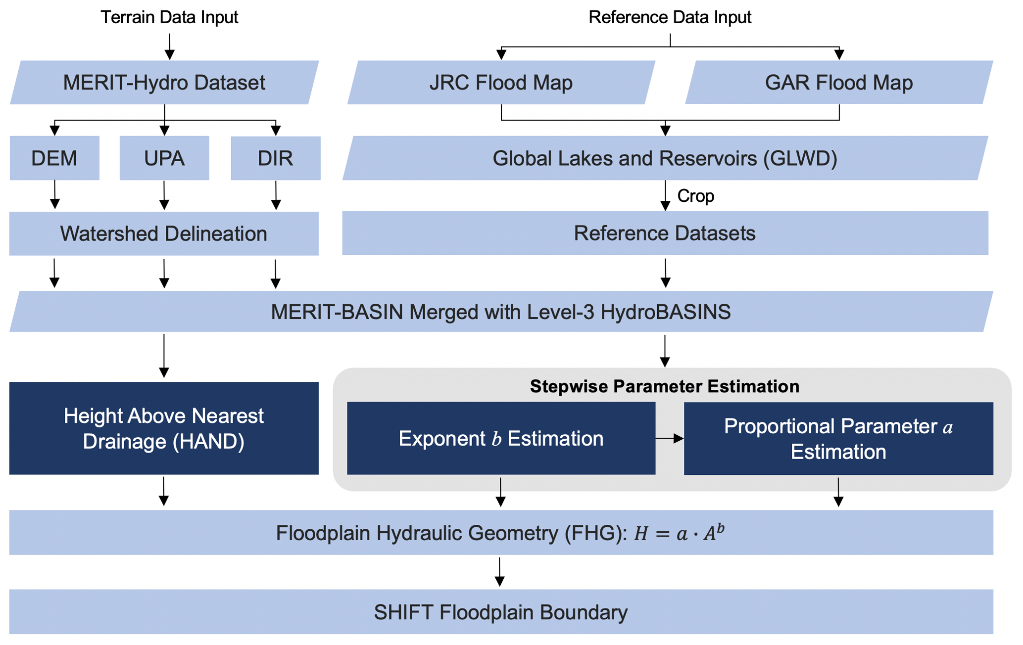
Figure 1 Technical workflow of the study. Parallelograms denote data; rectangles denote processing; highlighted rectangles are the key features of SHIFT. Stepwise parameter estimation is marked in the gray box.

To complement existing studies, here, we develop a globally applicable framework to estimate FHG parameters that better integrates spatial heterogeneity into our thresholding scheme. It takes two publicly available hydrodynamic floodplain maps as the reference to estimate spatially varied FHG parameters across all global river basins at the scale of the level-3 HydroBASINS. Based on this, we develop a 90 m global geomorphic floodplain map named the Spatial Heterogeneity Improved Floodplain by Terrain analysis (SHIFT). SHIFT calculates HAND above the nearest river pixel to which it drains by utilizing the hydrologically corrected MERIT Hydro (Yamazaki et al., 2019) dataset. Due to the use of the MERIT Hydro dataset, SHIFT also addresses limitations in the existing global geomorphic mapping that uses an uncorrected digital terrain model (DTM) with limited spatial coverages (60° N to 60° S) and relatively low spatial resolutions. Our article is organized as follows: Section 2 introduces our methods and data in detail. Section 3 presents our geomorphic floodplain data and the accuracy assessment against several reference maps. Sections 4 and 6 close with a discussion and the conclusions of this study.

2 Methods and data

SHIFT is developed following the technical flowchart in Fig. 1. Below, we will describe our data and methods in detail.

2.1 Data

2.1.1 Terrain data

1. MERIT Hydro hydrography map. We take terrain inputs (i.e., elevation, D-8 flow direction, and upstream drainage area) from the MERIT Hydro dataset (Yamazaki et al., 2019). It is a 90 m resolution global dataset that combines data from the Space Shuttle Radar Topography Mission (SRTM) and airborne lidar, which has undergone rigorous error correction processes to remove various types of errors such as striping noise, speckle noise, absolute errors, and biases in tree heights. Multiple remote sensing datasets and volunteer geographic information system (Volunteer GIS) water data are used to further enhance its ability to identify river locations. Specifically, it combines OpenStreetMap river vector data, SRTM waterbody data, and Landsat-derived water data to calculate the likelihood of a grid cell representing a water body. In areas with a high likelihood of water, the elevation is adjusted to be lower. This approach effectively improves the accuracy of flow direction calculations and minimizes deviations in flat areas. The dataset is georeferenced to the WGS84 and EGM96 geodetic reference systems, with a spatial resolution of 3 arcsec (approximately 90 m at the Equator).

2. HydroBASINS global basins. We applied basin boundary data from the level-3 HydroBASINS dataset to introduce the basin-by-basin spatial variability in parameter estimation. This is a multi-level global basin dataset derived from the SRTM DEM data as part of the HydroSHEDS project (Lehner and Grill, 2013). HydroBASINS is structured into 12 levels of basins, with higher levels representing finer basins. The dataset applies the Pfafstetter coding system to support the analysis of watershed topology, including upstream and downstream connectivity. The first three levels are assigned, with level 1 categorizing continents, level 2 dividing continents into major sub-units, and level 3 delineating the largest river basins on each continent (Lehner and Grill, 2013). The level-3 sub-basins in HydroBASINS consist of 269 units globally, with an average size of 555 600 km². Level-4 and level-5 boundaries are also applied for further analysis on scales.

3. MERIT-Basins. MERIT-Basins is a global vector hydrography database derived from the 90 m MERIT Hydro product, based on a 25 km² threshold for drainage areas (Lin et al., 2019). It aligns well with the MERIT Hydro dataset. To obtain the corresponding boundaries for parameter estimation, we combined MERIT-Basins into groups equivalent to level 3 to level 5 of HydroBASINS. We aggregated MERIT-Basins based on its spatial relationship with basins from HydroBASINS, ensuring that the centroid of a MERIT-Basin falls within the corresponding boundary. This approach accounts for slight differences in boundaries due to the use of different terrain data, preventing confusion in hydrological representation. Among the level-3 basins, the 40 largest hydrologically connected basins were manually selected based on the hypothesis that connected basins better apply the scaling law due to shared attributes within the same hydrological system. A total of 7 of these 40 basins, with centroids located above 60° N, were excluded since one of our reference maps does not cover regions above 60° N.

2.1.2 Reference and benchmark datasets

1. JRC flood map. The flood hazard map created by the European Commission's JRC is selected as part of the reference and validation dataset. It is based on the 3 arcsec SRTM DEM, which combines hydrological simulations from the Global Flood Awareness System (GloFAS) with a two-dimensional CA2D hydraulic model for flood inundation mapping. The GloFAS simulations utilize ERA-Interim data, covering the period from 1980 to 2013, and operate at a resolution of 0.1° (approximately 11 km at the Equator). The system simulates streamflow by coupling two distributed global models: HTESSEL, which estimates surface water and energy fluxes in response to atmospheric forcing, and the LISFLOOD Global, which uses the output from HTESSEL to simulate routing processes and streamflow. The flood hazard maps produced are at a 30 s resolution and focus on river channels with an upstream catchment area greater than 5000 km² (Dottori et al., 2016). The JRC dataset provides flood hazard maps with different return periods from 10 to 1000 years. Here, we used the 500-year flood map as a reference floodplain map based on the notion that geomorphic floodplains are dominantly shaped by high-impact yet low-possibility events (Annis et al., 2019; Bhowmik, 1984; Lindersson et al., 2021).

2. GAR flood map. We also select the 500-year flood map of the hydrodynamic model from the GAR of the United Nations Office for Disaster Risk Reduction (UNDRR) and the CIMA foundation as a reference and validation dataset. The GAR data employ a global database of discharge data from over 8000 stations to estimate extreme streamflows and a DEM from HydroSHEDS for hydraulic modeling. This one-dimensional model applies Manning's equation to calculate river stages. The GAR flood map also considers artificial flood defense by assuming target return periods of flood defenses based on the GDP distribution, thereby locally reducing the estimated flooded volume within the estimated protected area. The dataset is characterized by return periods of 25, 50, 100, 200, 500, and 1000 years, a coverage of 60° N to 60° S, with a native resolution of 90 m from the SRTM DEM, later aggregated to 1 km for risk computation (Rudari et al., 2015).

3. GFPLAIN250m floodplain map. The aforementioned geomorphically delineated GFPLAIN250m floodplain map is used as the benchmark and another validation dataset (Nardi et al., 2019). It has the same coverage as GAR (60° N to 60° S). For each grid, it calculates the height above the lowest elevation grid within the same watershed (i.e., the basin outlet) as the terrain attribute rather than the nearest river grid to which it drains. This exaggerates the vertical distance to streams for upstream pixels and may thus lead to underestimation of the floodplain. FHG is applied as the thresholding scheme (Nardi et al., 2006), but the exponent takes universal values across different basins (i.e., exponential parameter b = 0.3, proportional parameter a = 0.01) for convenient global applications. It takes the 250 m SRTM DTM as terrain input and implements the hydrological analysis workflow by using the ArcPy library.

4. Global Lake and Wetland Dataset (GLWD) lake and reservoir dataset. We apply a global lake mask to crop the reference map before using it for parameter estimation, which helps to avoid inconsistent lake representations from our reference and validation datasets. To do that, the Global Lake and Wetland Dataset (GLWD), jointly developed by the World Wildlife Fund (WWF) and the Center for Environmental Systems Research at the University of Kassel (Lehner and Döll, 2004), is used. It consists of three layers, and the level-1 layer represents large lakes and reservoirs, including 3067 lakes and 654 reservoirs with lake area ≥ 50 km² and storage capacity ≥ 0.5 km³, respectively. The dataset takes its reference from multiple sources and is further refined with independent data from USGS and extensive visual inspections and quality-controlling.

2.1.3 Datasets for correlation

1. Global-AI_PET_v3 aridity index database. We use the aridity index (AI) from the Global Aridity Index and Potential Evapotranspiration Database (Global-AI_PET_v3) to assess its linkage with the FHG parameter. The database provides 30 arcsec global potential evapotranspiration (ET₀) and AI data. AI is calculated as the ratio of the mean annual precipitation to the mean annual reference ET₀, which is estimated by the FAO Penman–Monteith Reference evapotranspiration equation. It has been validated against various weather station data and shows an improved correlation with real-world data compared to previous versions (Zomer et al., 2022).

2. Leaf area index (LAI) climatology. Developed for a model intercomparison project (HighResMIP v1.0) of CMIP6, this dataset provides a global 0.25° × 0.25° gridded monthly mean leaf area index (LAI) climatology, averaged from August 1981 to August 2015 (Haarsma et al., 2016). Derived from the Advanced Very High Resolution Radiometer (AVHRR) Global Inventory Modeling and Mapping Studies (GIMMS) LAI3g version 2, it includes bi-weekly data from 1981 to 2015. The raw LAI3g version 2 data were regridded from $\mathrm{1}/\mathrm{12}$° × $\mathrm{1}/\mathrm{12}$° to 0.25° × 0.25°, processed to remove missing and unreasonable values, scaled to obtain LAI values, and averaged bi-weekly to monthly. The final product is a monthly long-term mean LAI (1981–2015) provided in a single NetCDF (.nc4) file.

2.2 Methods

This section introduces HAND, FHG and our parameter estimation scheme for SHIFT.

1. HAND as a terrain attribute. HAND is a derivative terrain index that describes the relative elevation difference between any grid cell in a DEM and its nearest river grid (Rennó et al., 2008). Here, the river grid is identified by applying a 1000 km² threshold to the upstream drainage area (UPA), supported by previous studies (Nardi et al., 2019). The threshold is determined by preliminary experiments to ensure that it is neither too small, which would mis-attribute large-river-dominated floodplains to small rivers, nor too large, which would overlook rivers with notable influence. Accurate HAND calculation requires defining the nearest river network grids either by flow direction or by distance. The flow direction model defines the first river network grid reached by tracing the D-8 flow as the nearest drainage, resulting in floodplain maps that capture regional hydrological characteristics but that are influenced by local terrain fluctuations. The distance model searches for the nearest drainage grid within a specific distance (e.g., two-dimensional or three-dimensional Euclidean distance), highlighting geometric considerations, but ignores natural geomorphic separations. We adopt the flow direction method to avoid discontinuities in HAND introduced by the distance model (not shown); subsequent results in floodplain delineation are derived from using the D-8 flow directions obtained from the MERIT Hydro dataset.

2. FHG as a thresholding scheme. FHG is an adapted form of the original river channel hydraulic geometry (Leopold and Maddock, 1953). It posits a power-law relationship between floodplain characteristics (width, depth, 100-year discharge) and river size (UPA or Strahler stream order). In the context of floodplain delineation, it considers a power-law relationship between the potential inundation depth (h) of a river grid cell and its UPA:

   $$\begin{array}{}\text{(1)}& h=a\cdot {\mathrm{UPA}}^b,\end{array}$$

   where a and b are empirical parameters containing heterogeneous factors determining floodplain extents. Then, the algorithm determines grid cells with HAND lower than h for the corresponding river grid (h_river) to be floodplain, which can be represented by Eq. (2):

   $$\begin{array}{}\text{(2)}& f(\mathrm{HAND},h_{\text{river}})=\left\{\begin{array}{l}\mathrm{1},\mathrm{HAND}\le h_{\text{river}}\\ \mathrm{0},\mathrm{HAND}>h_{\text{river}}\end{array}\right..\end{array}$$

3. FHG parameter estimation. Estimating FHG parameters requires either reference floodplain extents or estimated runoff as inputs (Annis et al., 2019; Nardi et al., 2013). We take two hydrodynamic model outputs as the reference map (i.e., the 500-year return period JRC and GAR flood maps) as they intrinsically contain floodplain spatial heterogeneity by feeding gauged streamflow observations or climate reanalysis data (Lindersson et al., 2021). The goal of using these reference datasets is to capture information regarding the spatial heterogeneity of these two datasets while trying our best to constrain model-related uncertainties.

   With the above reference map, two methods can be used to estimate FHG parameters: parameter space sampling (PSS) and logarithmic regression (LR). PSS defines a feasible range for two parameters in Eq. (1) and then samples the parameters from the parameter space and tests their combinations against a reference map by using a fitness index (Annis et al., 2019). LR assumes that all floodplain grids from the reference map satisfy the scaling law so that the FHG parameters b and a can be estimated by statistical approximation (Nardi et al., 2013). For LR, we expect all floodplain pixels in the reference map to satisfy the following:

   $$\begin{array}{}\text{(3)}& \mathrm{HAND}\le a\cdot {{\mathrm{UPA}}_{\mathrm{river}}}^b,\end{array}$$

   which could be transformed into

   $$\begin{array}{}\text{(4)}& \ln \left(\mathrm{HAND}\right)\le b\cdot \ln \left({\mathrm{UPA}}_{\mathrm{river}}\right)+\ln \left(a\right).\end{array}$$

   Apparently, PSS can best approximate the output but could lead to equifinality, while LR emphasizes the scaling law but could be influenced by uncertainties in the reference data (see more details below). Therefore, we combine the two methods above and propose a stepwise parameter estimation framework. Specifically, we first determine baseline values for parameter a₀ from prior research, and then we estimate b by forcing logarithmic regression based on the reference dataset to best respect the FHG scaling law; following this, the coefficient a is calculated by sampling the parameter space based on the reference map and the determined b value.

   Equation (4) predicts a positive linear relationship (see Fig. 2a) between ln (UPA_river) and the maximum ln(HAND) values, which represent the most distant floodable grid for each river grid. However, our observations do not align with this expectation. This discrepancy occurs because some river grids with small drainage areas can exhibit unexpectedly high HAND values. These can be ascribed to uncertainties within our reference map, which inherits the model chain errors, terrain data, and spatial resolution inconsistencies, as well as other unaccounted within-basin variabilities that may break the scaling law. While results from the Gaussian kernel density plot (Fig. 2b) prove that the majority of data still conform to the power law, the patterns indicate that one cannot simply apply LR to the maximum ln(HAND) and ln (UPA_river) to obtain the required parameters.

   Therefore, we develop a scheme to effectively mitigate data noises in estimating parameter b while maintaining the power law for the majority of grids. First, we take floodplain grids from the intersection of the two reference maps as we suggest the intersection map to be more accurate. Then we set a universal HAND threshold of 20 m to screen out the most obvious high anomalies. We then group HAND values by UPA_river and apply an iterative moving-window data-filtering scheme based on 3σ statistics, where every grid would be filtered by 20 windows (window size = 1, step = 0.1). In each iteration, we compute the mean and standard deviation for the data within each window. A grid point is retained only if it consistently meets the 3σ criteria across all 20 windows. This iterative process stops either when every data point fits within all moving windows or if the procedure fails to converge towards a stable solution (e.g., for highly noised or significantly non-normal data). Instead of directly performing LR, we calculate a sequence of theoretical b values from the maximum HAND of each UPA_river unit with a baseline estimate of a₀ = 0.01 based on prior research (Nardi et al., 2019). The binning parameter is tuned to effectively reduce data noise for all basins. As the optimal b will lean towards the higher end of our calculated sequence but will not be at the highest end as it could possibly be interfered with by the remaining high HAND anomalies, we evaluate the 10 % to 50 % percentiles of these b sequences across all basins to identify the best percentile that centers around the previously estimated global b value of 0.3 (Nardi et al., 2019). The b value under this identified percentile is then chosen as the optimal parameter for each individual basin.

   After b is determined, the coefficient a is optimized with an iterative PSS method. We take both hydrodynamic maps as our reference dataset as we would like to highlight the “consensus” of existing maps while trying to achieve better consistency from both maps. Numerous indices for the optimization target exist, including overall accuracy (OA), the kappa coefficient (Cohen, 1960), Fleiss's kappa (Fleiss, 1971), the model agreement index (MAI, Trigg et al., 2016), or the measure-of-fit function (Nardi et al., 2019). While the MAI and measure-of-fit function emphasize data overlap, they do not address overprediction. OA considers unpredicted areas but may overly reward non-floodplains since they are the major landmass type. Fleiss's kappa can assess agreement among multiple datasets, but using it alone with two existing datasets may bias our estimated boundary towards the dataset with larger predictions as it maximizes mathematical consistency values. This is undesirable since we aim for agreement with each individual dataset to balance the information from both. Therefore, our target function is defined as follows:

   $$\begin{array}{}\text{(5)}& \mathrm{Consistency}=\mathrm{FK}-\mathit{\sigma }\cdot ({\mathrm{MAI}}_{\mathrm{JRC}}-{\mathrm{MAI}}_{\mathrm{GAR}}{)}^{\mathrm{2}}.\end{array}$$

   Here, Fleiss's kappa (FK) represents how well the three datasets (including the product with the parameter to be optimized) match. The penalty term, based on the squared difference between the two MAI values, reduces bias towards one dataset over the other. The weight term (σ), ranging from 0 to 1, is determined by the normalized number of available reference data grids in the basin. This assumes that basins with fewer common data grids have less reliable datasets; thus, overemphasizing the penalty term would unnecessarily and overly influence FK.

   Fleiss's Kappa (FK) is calculated as follows:

   $$\begin{array}{}\text{(6)}& \mathrm{FK}={\displaystyle \frac{P_{\mathrm{o}}-P_{\mathrm{e}}}{\mathrm{1}-P_{\mathrm{e}}}},\end{array}$$

   where P_o and P_e are, respectively, calculated by

   $$\begin{array}{}\text{(7)}& {\displaystyle }& {\displaystyle }{P}_{\mathrm{o}}={\displaystyle \frac{\mathrm{1}}{N}}\sum _{i=\mathrm{1}}^N{\displaystyle \frac{\sum _{j=\mathrm{1}}^C{n}_{ij}(n_{ij}-\mathrm{1})}{K(K-\mathrm{1})}},\text{(8)}& {\displaystyle }& {\displaystyle }{P}_{\mathrm{e}}=\sum _{j=\mathrm{1}}^C{\left({\displaystyle \frac{\sum _{i=\mathrm{1}}^K{n}_{ij}}{NK}}\right)}^{\mathrm{2}}.\end{array}$$

   In these equations, K is the number of models (three here), N is the number of pixels, i represents each grid, and j represents different possible values (1 or 0 here). The MAI is calculated as follows:

   $$\begin{array}{}\text{(9)}& \mathrm{MAI}={\displaystyle \frac{A}{A+B+C}},\end{array}$$

   where A, B, and C denote overlapping (true positive), over-prediction (false positive), and under-prediction (false negative), respectively. Considering the fact that the previously estimated a values range from 0.001 to 0.06 (Nardi et al., 2018), we first sample 20 equidistant a values between 0 and 1 against the reference data. Then the direct neighbor of the best-performing a value, constraining its precision to at least one decimal place, is used to search for the true optimal a. We apply five iterations, each with a new set of 20 equidistant a values within the estimated direct neighbors from the last iteration. The optimal a from the final iteration is then selected as the basin-specific coefficient.

4. Development of SHIFT. Based on the above, we estimate the FHG parameter with the HydroBASINS level-3 basins, and we derive the floodplain maps for each basin and then integrate them into a 90 m global floodplain map. We use Python 3.10 libraries (e.g., pandas, NumPy, and GeoPandas), the GDAL command line interface, and the TauDEM toolkit (Tarboton, 2016) for the FHG parameter estimation and the thresholding. We also downsize the dataset to a 1 km resolution floodplain map for convenient large-scale applications – the 1 km resolution floodplain map is provided as part of the final output. We used the median as the resampling method for continuous variables like UPA and HAND and the mode for categorical data, such as the reference maps, SHIFT, and watershed division. Permanent waterbodies are removed for all processes.

5. Validation and correlation. After getting the updated floodplain boundary with the optimized parameters (SHIFT), we conduct a pairwise consistency analysis among five maps, i.e., SHIFT, GFPLAIN250m, UPs (universal parameters, applying b = 0.3 and a = 0.01 in MERIT Hydro), JRC, and GAR. UPs were generated to allow the assessment of how changes in parameters influence the results. We apply both MAI (see Eq. 9) and OA for this pairwise consistency analysis in reference to previous research (Lindersson et al., 2021). Note that MAI is a critical index: an MAI of 0.2 represents 20 % to 33 % overlap between models, while an MAI of 0.5 represents 50 % to 67 % overlap. Previous large-scale assessments of floodplain map consistencies revealed that the median MAI is in the range of 0.1 to 0.4 (Lindersson et al., 2021). OA is calculated as follows:

   $$\begin{array}{}\text{(10)}& \mathrm{OA}={\displaystyle \frac{A+D}{A+B+C+D}},\end{array}$$

   where D denotes non-prediction by both maps, and A, B, and C are as defined in Eq. (9). The two types of indices applied here have different focuses: OA considers non-floodplain areas, while MAI focuses exclusively on overlapping floodplain areas. Considering the overall land mass is non-floodplains, we also calculated OA within 20 km buffer zones, with distance measured as the hydrological distance to the stream. In the pairwise comparison, group comparisons were conducted with JRC and GAR, where each hydrodynamic map was tested against SHIFT, GFPLAIN, and UPs. The JRC–GAR pair serves as the baseline.

   For our analysis, we focus on parameter b. Theoretically, b influences rivers differently based on their drainage area, with larger b values highlighting the dominance of large rivers over tributaries in shaping floodplain extents. Thus, we expect b to be closely associated with the spatial heterogeneity of basin-level hydrological and geomorphic characteristics. Our primary hypothesis is that b should be related to climate aridity as more humid areas are expected to show a stronger dominance of large rivers. Additionally, vegetation, indicated by LAI (leaf area index), may also play a role since it is involved in the runoff generation process, as well as in modulating soil erosion, which can be key to floodplain formation. Therefore, we calculate the correlation of b with average AI (aridity index) and LAI across all basins to validate whether our thresholding scheme can better capture the spatial heterogeneity of floodplain characteristics.

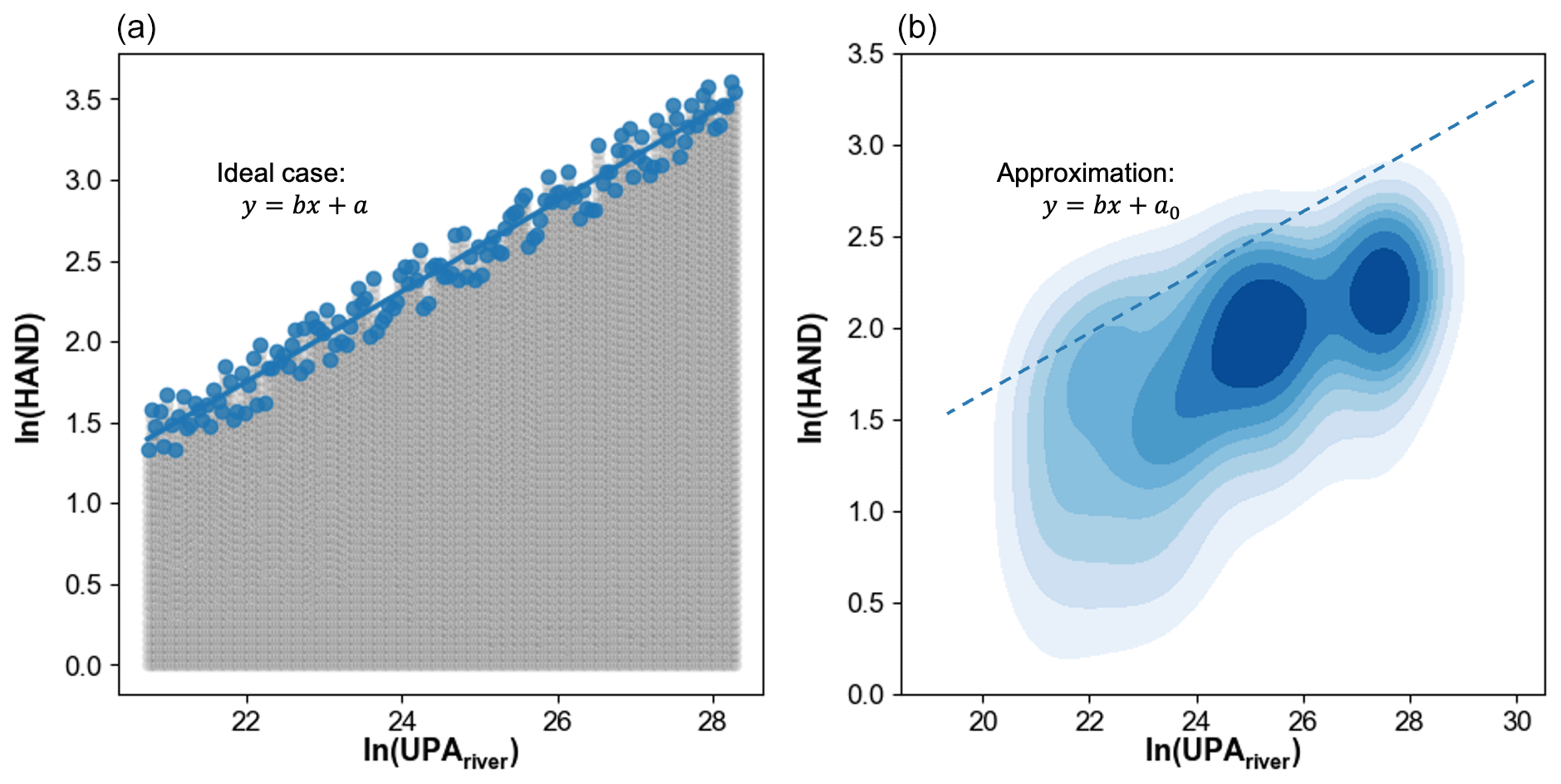
Figure 2 The expected and actual scenario of floodplain grids within a basin. The x axis represents ln (UPA_river), and the y axis represents ln(HAND). Panel (a) shows the scatterplot of the expected linear relationship between maximum ln(HAND) and ln (UPA_river). Blue scatters are the maximum HAND values, while gray scatters are non-maximum reference floodplain grids. Panel (b) shows an actual scenario (i.e., the Yangtze River basin corresponding to the level-3 HydroBASINS, PFAF ID no. 434) which approximately arrives at the power-law relationship in the kernel density plot.

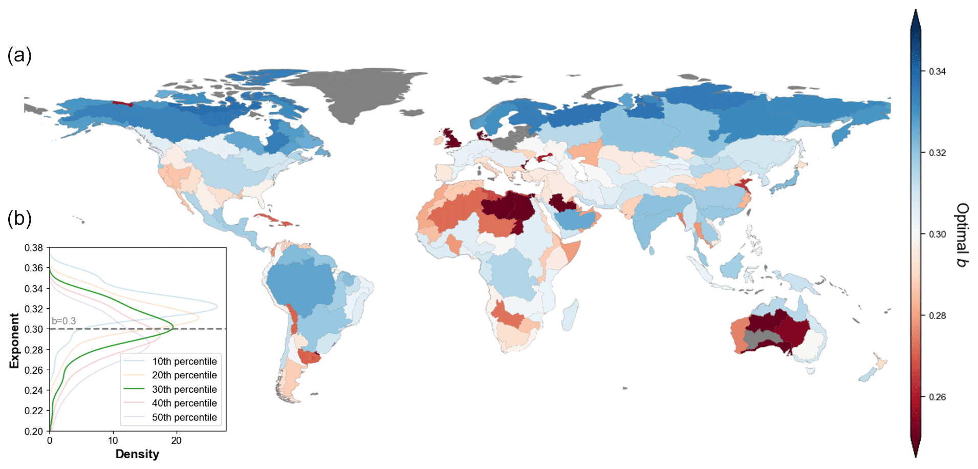
Figure 3 Statistical and spatial distribution of estimated FHG parameter b. (a) Spatial distribution of parameter b across HydroBASINS level-3 basins. (b) The distribution of parameter b across basins; p₁₀ to p₅₀ represent the percentiles during estimation, and the b = 0.3 line shows the universal value applied in previous research.

3 Results

3.1 Global FHG parameter estimation

Following the stepwise parameter estimation scheme proposed in Sect. 2.2 (3), we obtain the statistical distributions of different b percentiles in Fig. 3b. While distributions from all percentiles exhibit similar patterns, especially for the 20th to 50th percentiles, we apply the 30th percentile worldwide as it distributes best around the previously estimated global b value of 0.3 (Nardi et al., 2019; see dashed line in Fig. 3b). The majority of estimated parameter b values lie within the range of 0.25 and 0.35. Based on the estimation, the coefficient a is also optimized, varying from 0.0001 to a maximum of 0.12 across all basins.

Spatially, the distribution of the estimated b (Fig. 3a) shows that regions characterized by abundant precipitation and water resources (e.g., southern East Asia, Southeast Asia, and the Mississippi and Amazon river basins) generally exhibit relatively higher b values. Conversely, regions such as central western Asia, the Arabian Peninsula, the Sahara region, and central Australia tend to have relatively lower b values. There are also exceptions: for instance, the overall high b values in the Arctic Circle and the low values in river deltas (e.g., the western Mississippi Delta in Louisiana and Jiaodong Peninsula in eastern Asia). The estimated parameter a exhibits a less clear spatial pattern (Fig. S1 in the Supplement) as it is less uniform in terms of unit and is highly dependent on the estimated b value.

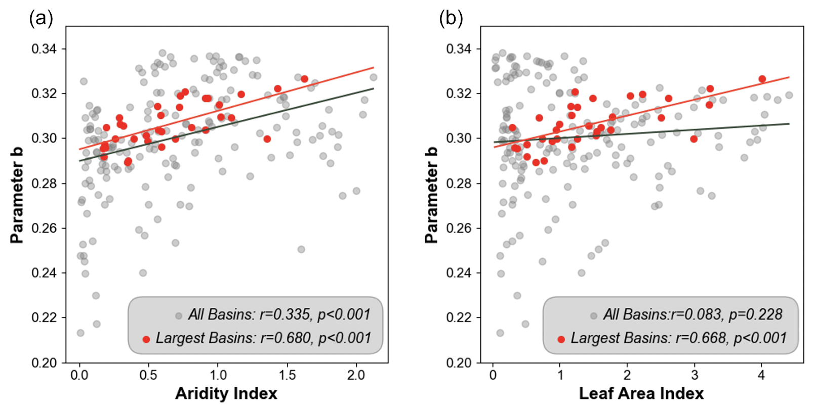
Figure 4 Scatterplots of FHG parameter b against relevant hydroclimatic factors. (a) Scatterplot with AI (aridity index). (b) Scatterplot with LAI (leaf area index). In each plot, gray points represent all basins, including the largest ones, while red points represent the 33 selected basins. Pearson's r and significance levels are indicated on the plots.

Statistically, results show that b from all basins exhibits significant but weak positive correlations with the AI (aridity index, r = 0.335, Fig. 4a) and an insignificant positive correlation with LAI (leaf area index, r = 0.083, Fig. 4b). For the selected 33 major basins, which are hydrologically connected and thus expected to have more internally consistent hydrological characteristics, both correlations are stronger (r = 0.680 for AI and r = 0.668 for LAI) and significant. We investigate other potentially relevant factors (Fig. S1), but no significant and consistent linear correlations were observed, suggesting that more complex mechanisms may be involved that do not manifest as observable linear correlations.

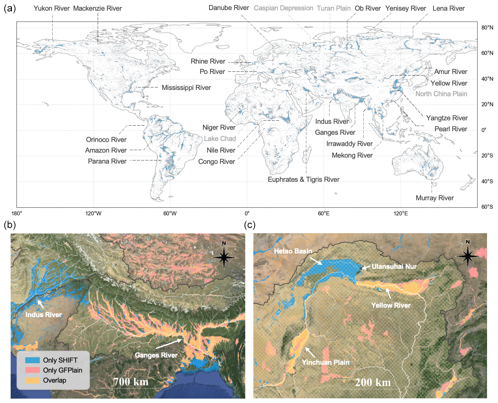
Figure 5 Geomorphic floodplain extent in SHIFT. (a) Global spatial distribution of floodplains, with major river basins or plains marked out. (b, c) Two cases comparing SHIFT with GFPLAIN250m, with the background image from © Google Earth on EPSG: 3857 projection. Panel (b) is located in the humid Indus and Ganges–Brahmaputra river basin, while panel (c) is located in the semi-arid Yellow River basin in Inner Mongolia, China. Major rivers of the region are marked on the map. SHIFT delineates fewer areas in the upstream Ganges River (b) and reduces the floodplain extent outside the Yellow River main stream (c). It also offers more comprehensive coverage, including the Indus River basin (b) and the Hetao Basin (c).

3.2 Global floodplain delineation

Based on the estimated FHG parameters, the global distribution of floodplain areas is delineated and shown in Fig. 5a. Overall, the spatial pattern of the floodplains aligns well with the low-lying areas in major river systems. More specifically, floodplains in northern Asia are mainly distributed around the western Siberian Plain and the central western Siberian Plateau, e.g., the Ob and Yenisei River basins. Western and central Asia's floodplains are primarily near the Caspian Sea, the Aral Sea, and the Mesopotamian Plain. In East Asia, the Yangtze River Basin dominates floodplains in the middle and lower reaches, along with contributions from the North China Plain, some Yellow River tributaries such as the Hetao Plain, and river mouths in the southeast. The Lancang–Mekong River basin and the Salween–Irrawaddy River basin in Southeast Asia also breed the largest floodplains worldwide, along with the Indus and Ganges–Brahmaputra River basins from southern Asia. In Europe, the primary floodplains are concentrated in the Danube River basin between the Alps and the Carpathian Mountains, alongside the Rhine, Dnieper, and Po River basins. In Africa, floodplains are predominantly distributed in the upstream Nile River, including the Nile Delta and the Niger River basin, as well as in the Congo River Basin, in the Chari River–Lake Chad basin, and around Lake Victoria, with additional areas near western and eastern Africa's coasts. North America's floodplains are mainly in the Mississippi River basin and Alaska's Yukon River basin. South America's floodplains are primarily in the Amazon River basin, the Orinoco Plain, and the La Plata Plain. In Oceania, floodplains center in the interior lowlands around the Murray–Darling River basin.

To show more regional details, we use two cases with different climatic conditions (Fig. 5b and c) to further illustrate the differences between SHIFT and the widely used GFPLAIN250m dataset. Case 1 (Fig. 5b) is the Indus–Ganges–Brahmaputra River basin, which flows through Bangladesh, India, Pakistan, and Nepal. These countries are primarily characterized by frequent floods and are strongly influenced by the south Asia monsoon. SHIFT captures detailed floodplains in the Indus River basin, a major basin in southern Asia which GFPLAIN250m leaves out. Additionally, SHIFT offers finer details in upstream areas and can better distinguish main river floodplains from those of the tributaries. Case 2 (Fig. 5c) is situated in the Yellow River basin (Hetao Plain) in Inner Mongolia, China, a region dominated by arid to semi-arid continental climate. Comparing the floodplain maps with visual interpretations of the satellite images suggests that SHIFT can provide a more comprehensive depiction of the Hetao Plain. The floodplains outside of the Hetao Plain in SHIFT are relatively limited, which aligns with its generally dry climate conditions.

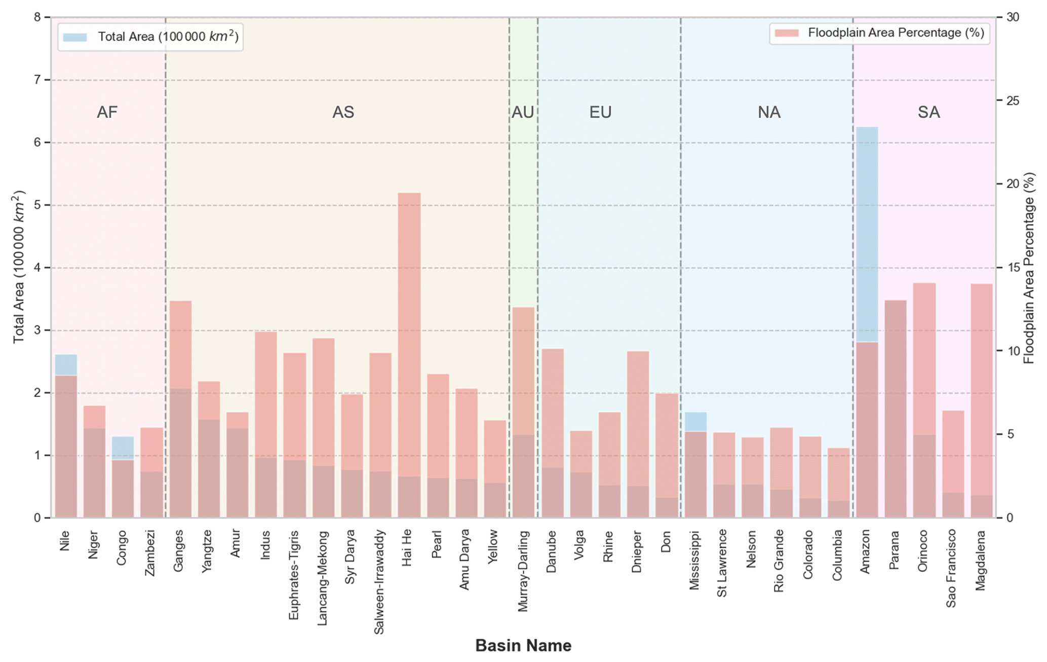
Figure 6 Floodplain area statistics in major river basins. Blue bars stand for total floodplain area (left y axis), and red bars stand for the ratio of floodplain area to the total basin area (right y axis). Basins are ranked by total floodplain area. AF: Africa, AS: Asia, AU: Australia, EU: Europe, NA: North America, and SA: South America.

According to SHIFT, global floodplains take up approximately 9.91×10⁶ km², representing 6.6 % of the world's total land area. Figure 6 further shows the floodplain area and the percentage of floodplains within each of the global major river basins. Overall, the Amazon River basin possesses the largest total floodplain area globally (625 431.3 km²), followed by the Paraná, Nile, Ganges, and Mississippi River basins. Floodplains in the Haihe River basin take up the greatest area percentage (∼ 20 %), highlighting the great geomorphic flood inundation potential of such basins. Comparing across continents, South America and Asia breed the most widespread floodplain extent worldwide and tend to have the highest floodplain percentages.

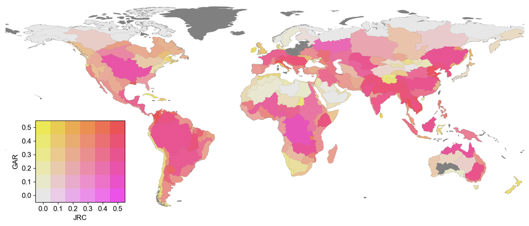
Figure 7 Validation of SHIFT against two reference datasets. In the bivariate map, the two variables are the MAI against the JRC map (magenta) and the GAR map (yellow). A balanced MAI results in red basins.

3.3 Validation and consistency analysis

Figure 7 shows the basin-level distribution of MAI between SHIFT and the two hydrodynamic maps. It shows that (1) SHIFT exhibits stabler consistency with the two maps in major basins (e.g., the Yangtze and the Amazon) compared to smaller basins and that (2) better consistency between SHIFT and reference maps is found in humid basins, with some exceptions in arid areas (e.g., the Niger). These patterns may be attributed to the greater number of reference data grids in larger and wetter basins, which also have strong scaling relationships that support a geomorphic approach for floodplain mapping. In addition, SHIFT generally aligns better with JRC in major river basins, while consistency with GAR is higher in smaller basins and inland river basins. The median MAI with JRC is 0.271, while, for GAR, it is 0.308. For the 33 major basins, the median MAI values with JRC and GAR are 0.415 and 0.289, respectively. This difference can be ascribed to the different river stream delineation strategies adopted by the two datasets. That is, JRC uses a stream threshold of 5000 km² for drainage area, while GAR uses 1000 km². Consequently, JRC is less effective in capturing features of inland basins (e.g., the Tibetan Plateau) and fragmented river deltas (e.g., west of the Andes), where few rivers meet the 5000 km² threshold. For large basins, JRC performs better, as it highlights the inundation of larger rivers (e.g., the Mississippi), while, in GAR, small rivers also yield large floodplain extents. Notably, SHIFT generally aligns better with JRC for the Arctic basins as GAR lacks data north of 60° N.

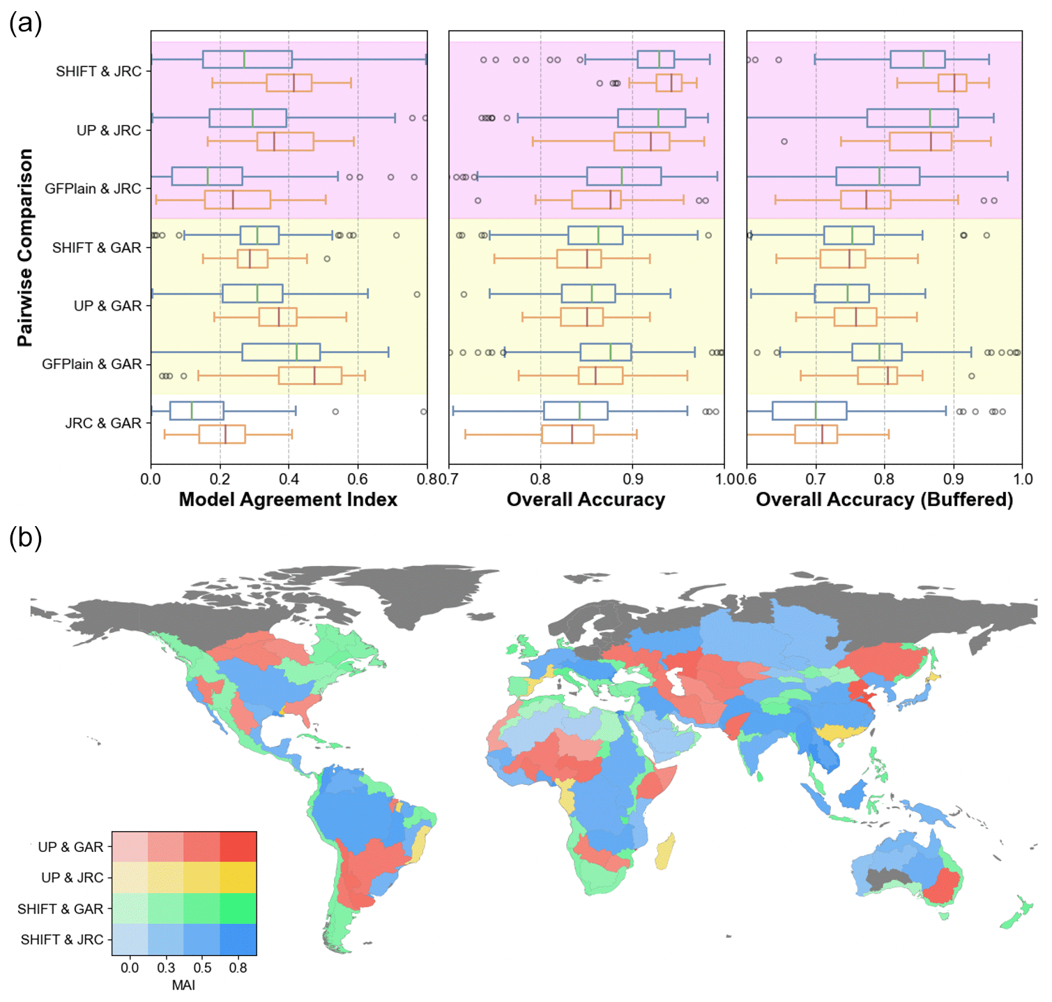
Figure 8 Results of the consistency analysis. (a) Boxplots of pairwise analysis among SHIFT, GFPLAIN, UPs (MERIT Hydro but with universal parameters), JRC, and GAR across three metrics: MAI (left), OA (middle), and OA within a 20 km buffer (right). Two group comparisons are marked in different colors (magenta for JRC and yellow for GAR). Statistics for all basins with valid data inputs (see “Methods and data” section) are shown in blue boxes, and those for the 33 major river basins are shown in orange. (b) Bivariate choropleth map of the highest-performance MAI pair among four pairs (SHIFT and JRC, SHIFT and GAR, UPs and JRC, UPs and GAR) and the corresponding MAI value for each basin. Different pairs are represented by different hues, with higher MAI values shown with a higher saturation. Basins where a SHIFT pair performs best are marked in cold colors, while those where a UP pair performs best are represented in warm colors. Among all pairs, SHIFT–JRC performed best in 62 basins, SHIFT–GAR performed best in 74, UP–JRC performed best in 8, and UP–GAR performed best in 37.

Figure 8a shows the pairwise consistency analysis among different floodplain maps to more objectively document the pros and cons of each dataset. Prominently, it shows that the consistency between SHIFT and JRC significantly improves over UP and GFPLAIN, but that with GAR does not (as shown in MAI). The consistency pattern can be explained by delving into the inner workings of each dataset. For large basins, SHIFT highlights the main streams and reduces the prediction of tributaries, thus aligning more closely with JRC as it highlights major rivers, leading to a decrease in consistency with GAR. UP and GFPLAIN align better with GAR in these regions as they all tend to overpredict, especially in tributaries. For other basins, SHIFT strikes a balance between the two datasets. Comparing SHIFT with UP, SHIFT increases the lower interquartile range for JRC's OA and the upper interquartile range for GAR's OA, highlighting a general improvement with SHIFT. For MAI, the upper quartile with GAR decreases, while the lower quartile improves, suggesting a consistency trade-off between the two datasets. Notably, all geomorphic maps show a better consistency with the hydrodynamic outputs than the hydrodynamic pair, proving again that the hydrogeomorphic delineation method is a more globally consistent framework.

To better understand the impact of our estimated parameters on the consistency performance, we analyze the most consistent pair and corresponding MAI values for each basin. Among all pairs, SHIFT–JRC aligns the best in 62 basins, with SHIFT–GAR aligning best in 74, UP–JRC aligning best in 8, and UP–GAR aligning best in 37 (Fig. 8b). This validates that SHIFT exhibits better consistencies with the reference maps even though the difference between SHIFT and UP seems to be not statistically significant (Fig. 8a). Spatial patterns (Fig. 8b) show that SHIFT–JRC pairs align best in humid major basins (e.g., the Mississippi and Amazon) and very arid regions (e.g., the Taklamakan and central Australia). SHIFT–GAR pairs are the most consistent in mountainous regions (e.g., the Rockies and Andes), aggregated deltas (e.g., eastern Australia and southern Africa), islands (e.g., Indonesia), and inland river basins (e.g., the Tibetan Plateau), where few rivers meet the 5000 km² drainage area threshold of JRC. In contrast, cases where UP pairs align best are less common. UPs align better with GAR due to their shared large prediction extents, such as around the Caspian Sea. In rare instances where UP–JRC pairs perform best, it is typically in deltas or regions where SHIFT–GAR performs well, such as deltas and islands. This is likely because our method balances consistency between the datasets, but GAR's wider prediction coverage makes this strategy less effective in these infrequent cases.

Note that GFPLAIN and UPs use the same parameters for geomorphic delineation, but their consistency with JRC and GAR differs significantly (Fig. 8a). This is because GFPLAIN uses 250 m SRTM as the terrain input, while UPs use MERIT Hydro, which has undergone hydrological correction to lower the elevation of waterbody pixels, resulting in higher HAND values and smaller floodplain extents. GAR, which generally overpredicts floodplain extents, especially in arid regions, aligns better with GFPLAIN. The overprediction of GAR is evidenced by GAR pairs having the lowest OA as OA strictly penalizes overprediction. At the same time, we found that the difference between SHIFT and UPs may be underrepresented in the statistical plots (Fig. 8a), while the actual impact of variable parameters brought about by SHIFT is substantial: the global floodplain extent estimates are 14.95×10⁶ km² for UPs and 9.91×10⁶ km² for SHIFT, showing a 50.85 % difference in total predicted areas. Additionally, regions where UP–GAR has the highest consistency (Fig. 8b) generally coincide with regions where SHIFT–JRC aligns best. This reversed pattern of consistency further supports the fact that the statistical differences between UPs and SHIFT are underrepresented in Fig. 8a.

4 Discussion

Several conceptual and technical details warrant discussion when developing our improved geomorphic parameter estimation approach. Here, we discuss the pros and cons of SHIFT with respect to its FHG thresholding scheme, residual uncertainty, hydrogeomorphic floodplain boundary, and the spatial scale used in our methodological development.

4.1 FHG as a thresholding scheme

The primary contribution of this study is the estimation of localized parameters for the FHG model. In Sect. 3.3, we compared the performance of localized versus global parameters, but several aspects require further clarification.

First, we believe the need for localized parameters arises from the role that empirical parameters in FHG play in determining floodplain boundaries. A higher b value emphasizes the influence of larger rivers in shaping geomorphic floodplains, reflecting hydrogeomorphic processes that vary across different basins, and should be better represented. Given the absence of ground truth for floodplain boundaries, we attempt to improve the representation of these heterogeneous processes by balancing information from two existing reference maps for hydrodynamic modeling. Despite acknowledged inconsistencies, the hydrodynamic maps are informed by climatic forcing, providing a common basis that is more likely to be spatially heterogeneous than universal geomorphic parameters. In other words, while we do acknowledge that these maps can be uncertain, they contain useful information that can be applied to constrain geomorphic floodplain boundaries. This leads to our data-filtering process to reduce inconsistencies and to identify a scaling law from the references. By incorporating outputs from hydrodynamic maps, our approach optimizes the DEM-based model without altering its foundation, as evidenced by the overall better consistency regardless of parameters used (Fig. 8a). Although certain regions may benefit less from our strategy (e.g., where UP–JRC performs best), results (Fig. 8b) show convincing general improvements and consistency patterns. The estimated parameters derived here are also provided to support potential future studies with regionalized focuses.

Second, our estimated parameters aim to capture fingerprints from spatially varying hydrological and geomorphic processes that can influence the floodplain extent. We consider aridity to be the primary factor influencing the spatial variability of b based on the assumption that, in humid basins, rivers with larger upstream drainage areas exert greater dominance over smaller segments in shaping floodplains. Vegetation also plays a role as it influences runoff generation and modulates soil erosion, both key to floodplain formation. Additionally, factors such as terrain and soil composition might influence the results. Given the data uncertainties and the complex physical interpretations of b, it is important to note that we do not expect perfect relationships between these factors and the derived exponent b. The correlation analysis indeed aligns with our expectations: AI is statistically significant in explaining the spatial variability of b, while LAI plays a role, and terrain does not show strong correlations with b. Soil compositions (Poggio et al., 2021) do not exhibit a consistent pattern across analyses done at different scales (Table S1 in the Supplement). Although the correlations between the b values and both AI and LAI are not strong, the statistical significance of these relationships supports the effectiveness of our proposed methods, which help to derive spatially varying parameters that are also physically meaningful. The parameter a could also encapsulate influences from relevant processes, but its physical interpretation is highly dependent on b as its unit is less uniform (Nardi et al., 2006). Therefore, clarifying the influencing processes of a is beyond the scope of this study.

Third, although alternative thresholding methods that use river discharge and synthetic rating curves exist (e.g., those used by the US National Water Model, Zheng et al., 2018), these methods come with more sources of uncertainty by requiring high-quality data inputs (e.g., gauged discharge, Manning's coefficient). Thus, while they may work well with in situ observations, replicating this globally poses challenges and is conceptually different from our approach. Our proposed FHG method requires only terrain input, which is recognized as the least uncertain component in the global floodplain-mapping method (Bates, 2023). By providing the optimized parameters derived here, we consider the FHG thresholding to be more globally consistent and easily applicable.

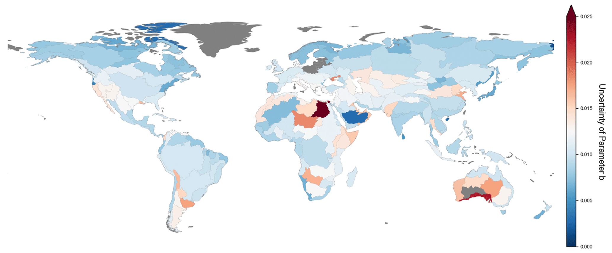
Figure 9 Spatial pattern of the residual uncertainty of parameter b by basin. Residual uncertainty is quantified as the standard deviation among all possible b values derived at different percentiles (see Sect. 2.2 for details).

4.2 Residual uncertainties associated with FHG parameter estimation

We also recognize several uncertainties associated with the FHG relation. The primary source of uncertainty comes from the inconsistency between the two reference hydrodynamic datasets across regions, which can be traced back to their model chain errors. Several measures are taken to mitigate the potential influence: we take the intersection of the two datasets as the reference, apply an iterative moving-window scheme to filter the data, and force scaling-law relationships to estimate the parameter b. However, residual uncertainties may still exist due to three aspects: (1) inconsistencies in terrain data as both JRC and GAR use SRTM as the inputs, while we use MERIT-Hydro; (2) potential intra-basin heterogeneity of scaling relationships, which may lead to unstable estimates; and (3) the lack of reference data in certain basins, which lowers our credibility with regard to the estimated parameters. To evaluate how the residual uncertainty influences our FHG parameter estimation, we quantify the uncertainty of b by calculating the standard deviation among all possible b values derived at different percentiles. This metric assesses how well the data conform to the power law: a better-conforming set of data results in a narrower range of the estimated b sequence and, consequently, a lower standard deviation. A lower standard deviation also supports the application of uniformly filtering percentiles globally (see “Methods and data” section) and proves the robustness of our approach.

Figure 9 reveals the residual uncertainty in parameter b, which ranges from 0 to 0.03, with a median of 0.01. This is considered to be reasonable for a global median b of 0.3. The pattern is similar to that of parameter b itself (Fig. 3), with lower uncertainties in large humid basins (blue color) and the greatest uncertainty (red color) observed in arid regions (e.g., the Saharan regions and western central Australia), mountainous areas (e.g., the Rocky Mountains and the Andes), and deltas (e.g., The Jiaodong Peninsula, the western Mississippi Delta, and the Nile Delta). High residual uncertainty in these regions is possibly due to the particularly strong differences between the reference datasets. For deltas, the great inconsistencies in spatial extents are amplified by their different definition of rivers as JRC and GAR, respectively, take up a stream threshold of 5000 and 1000 km². This also explains the unexpectedly low b values in deltas observed in Fig. 3. In contrast, the Arctic exhibits generally low uncertainty, likely because only one reference dataset is available above 60° N, reducing discrepancies and thus lowering the remaining uncertainty.

4.3 Floodplain definition and inundation maps

We also dedicate some discussion to the definition of floodplains here as numerous definitions exist for different intended uses. Geomorphically, a floodplain is an accumulation plain along a watercourse, formed by unconsolidated sediment transported and deposited by the stream, usually flooded during high flows (Brierley and Fryirs, 2013). This definition emphasizes the formation process. From a hydrologist or a flood manager's perspective, the floodplain is often associated with inundation attached to certain flood strengths (Krizek et al., 2006), which can also be referred to as the hydraulic floodplain. Alternatively, focusing on material flux exchanges yields different boundaries (Wohl, 2021). We consider these perspectives to be not contradictory but complementary in floodplain-mapping processes as they highlight different aspects of floodplains. Specifically, geomorphic floodplains are predominantly shaped by low-probability but high-impact flood occurrences (Lindersson et al., 2021), which subsequently connects our goal of delineating a geomorphic floodplain with identifying a boundary that encompasses all potentially inundated areas under extreme conditions. Therefore, we have used two 500-year return period flood maps as references for estimating our parameters in order to ensure a sufficiently large boundary for the carrying out of this algorithm. This way, the geomorphic definition of a floodplain is still obeyed. While the FHG parameters can be approximated for various return periods (Nardi et al., 2006), our approach does not focus on or involve a specific return period for inundation. In other words, our goal is not to provide a mere substitute for inundation maps. Instead, we aim to leverage a river's geographical characteristics and hydrological extreme conditions to identify scaling relationships that align with geomorphic principles and to offer a more comprehensive understanding of global floodplain extents.

4.4 Spatial scales of SHIFT

The spatially varying parameters for SHIFT are derived at the scale of HydroBASINS level-3 basins, which depict 269 river basins globally, with some containing aggregations of smaller basins. These aggregated basins are not hydrologically connected and are less suitable for our thresholding scheme, which estimates one set of parameters for each basin, compared to the largest basins, which share internally consistency hydrogeomorphic processes. A possible strategy to improve the scheme is to further divide these basins into smaller sub-basins, but smaller-scale analysis can increase the impact of reference data uncertainties, especially in delta regions with high floodplain discordance (Fig. 5a). Parameters for level-4 and level-5 basins were also calculated (statistics are given in Table S1), but many basins had insufficient reference grids to give reliable estimations. Considering the high data noise that may limit further integration of sub-basin-level heterogeneity in estimating parameters, the spatial disaggregation scheme used by SHIFT (i.e., level 3) is sufficient for improving heterogeneity while offering reasonable physical interpretations of the parameters.

Lastly, when calculating HAND as the terrain attribute for SHIFT, we set a UPA threshold of 1000 km² to delineate the river network grids following past studies (Nardi et al., 2019; Rudari et al., 2015). A sensitivity test on a smaller threshold (50 km²), not shown here, suggests that more detailed floodplains around smaller rivers can be derived, but, at the same time, such a threshold can limit the expected floodplains of large rivers. Conversely, a larger threshold, such as the 5000 km² one used by the JRC dataset, imposes a stricter criterion on river streams, leading to fewer river networks and reduced floodplain boundaries in areas like deltas. Thus, this study considers the 1000 km² UPA threshold to be valid. Future large-scale studies can further investigate the above-mentioned scale parameters, but we expect the gains to be minimal.

5 Code and data availability

SHIFT is openly available at https://doi.org/10.5281/zenodo.11835133 (Zheng et al., 2024). The core codes involved in terrain analysis and FHG parameter estimation are available at https://doi.org/10.5281/zenodo.13311752 (Zheng, 2024).

6 Conclusions

In this study, we develop an improved thresholding scheme for large-scale DEM-based floodplain delineation, the core of which is a stepwise estimation framework for floodplain hydraulic geometry (FHG) parameters that respects the power law while better integrating spatial heterogeneity from two publicly available hydrodynamic flood maps. We applied the framework at the scale equivalent to HydroBASINS level-3 basins to derive localized FHG parameters as an update to previously global parameters that do not account for the heterogenous factors influencing floodplain extents. The optimized empirical exponent b in FHG exhibits statistically significant positive correlations with hydroclimatic conditions, particularly in major river basins. Based on the proposed framework, we created a global geomorphic floodplain map named SHIFT (Spatial Heterogeneity Improved Floodplain by Terrain analysis) using terrain inputs from the 90 m MERIT Hydro dataset, where SHIFT is demonstrated to capture both the global patterns and the regional details of geomorphic floodplains well. The effectiveness of our framework is supported by the following:

1. The parameters show statistically significant but relatively weak relationships with hydroclimatic variables (e.g., AI, LAI), suggesting an enhanced representation of spatially heterogeneous hydrological and geomorphic information at the basin level.

2. The filtered data conform to a relatively stable power law, suggesting a robust regionalized scaling relationship.

3. Parameter changes lead to improved consistency with existing maps, with better differentiation between main streams and tributaries in major basins and more comprehensive representation of stream networks in aggregated river basins.

We provide the SHIFT data layers at two spatial resolutions (i.e., 90 m and 1 km) for the convenience of the users. The optimized parameters are also provided to support future studies.

Overall, we offer a framework for estimating spatially varying FHG parameters, contribute an updated geomorphic floodplain dataset, provide a better understanding of observable influences in the FHG scaling relationships, and expand on the discussion regarding the different focuses and implications of various floodplain-mapping techniques. We hope our analysis proves to be helpful in enhancing the understanding of current methodologies for defining and identifying active floodplains, especially in the context of changing climate.