Multisource Synthesized Inventory of CRitical Infrastructure and HUman-Impacted Areas in AlaSka (SIRIUS)

The Arctic region has undergone warming at a rate more than 3 times higher than the global average. This warming has led to the degradation of near-surface permafrost, resulting in decreased ground stability. This instability not only poses a primary hazard to Arctic infrastructure and human-impacted areas but can also lead to secondary ecological hazards from infrastructure failure associated with hazardous materials. This development underscores the need for a comprehensive inventory of critical infrastructure and human-impacted areas. The inventory should be linked to environmental data to assess their susceptibility to permafrost degradation as well as the ecological consequences that may arise from infrastructure failure. Here, we provide such an inventory for Alaska, a vast state covering approximately 1.7 × 10⁶ km², with a population of over 733 000 people and a history of industrial development on permafrost. Our Synthesized Inventory of CRitical Infrastructure and HUman-Impacted Areas in AlaSka (SIRIUS) integrates data from (i) the Sentinel-1/2-derived Arctic Coastal Human Impact dataset (SACHI); (ii) OpenStreetMap (OSM); (iii) the pan-Arctic Catchment Database (ARCADE); (iv) a dataset of permafrost extent, probability and mean annual ground temperatures; and (v) the Contaminated Sites Database and reports to create a unified new dataset of critical infrastructure and human-impacted areas as well as permafrost and watershed information for Alaska. The integration process included harmonizing spatial references, extents and geometries across all the datasets as well as incorporating a uniform usage type classification scheme for the infrastructure data. Additionally, we employed text-mining techniques to generate complementary geospatial data from textual reports on contaminated sites, including details on contaminants, cleanup duration and the affected media. The combination of SACHI and OSM enhanced the detail of the usage type classification for infrastructure from 5 to 13 categories, allowing the identification of elements critical to Arctic communities beyond industrial sites. Further, the new inventory integrates the high spatial detail of OSM with the unbiased infrastructure detection capability of SACHI, accurately representing 94 % of the polygonal infrastructure and 78 % of the linear infrastructure, respectively. The SIRIUS dataset is presented as a GeoPackage, enabling spatial analysis and queries of its components, either as a function of or in combination with one another. The dataset is available on Zenodo at https://doi.org/10.5281/zenodo.8311243 (Kaiser et al., 2023).

1 Introduction

In the past decades, the Arctic has experienced a pronounced warming, entailing an increase in air temperature that is more than 3 times higher than the global average (Rantanen et al., 2022), referred to as Arctic amplification (Cohen et al., 2014). These increasing air temperatures have led to warming and thawing of permafrost since the 1980s, as borehole measurements across the Arctic demonstrate (Biskaborn et al., 2019; Smith et al., 2022). Modeling studies indicate that the initiation of permafrost warming can be traced back to as early as 1900 (Langer et al., 2024). As 15 % of the exposed land surface of the Northern Hemisphere is underlain by permafrost (Obu et al., 2019), this warming trend affects a vast area and has major implications for ecosystems and livelihoods in the Arctic and sub-Arctic. With permafrost degrading, we expect not only the mobilization of one of the largest soil carbon pools (Schuur et al., 2015, 2022), but also substantial land surface changes that result from ground subsidence and thermal erosion (Kokelj and Jorgenson, 2013). Permafrost warming trends can also be observed in mountain regions worldwide (Biskaborn et al., 2019), leading to the destabilization of slopes and increased movement of rock glaciers (Haeberli, 2013; Haeberli et al., 2024). Numerous studies demonstrate intensifying land surface changes in the permafrost region which encompass, e.g., processes such as thaw slumping (e.g., Runge et al., 2022; Ramage et al., 2017; Leibman et al., 2021), the development of thermokarst ponds and lakes (e.g., Muster et al., 2017; Jones et al., 2011), thermoerosional gullying (e.g., Fortier et al., 2007; Godin et al., 2012), ice wedge degradation (e.g., Liljedahl et al., 2016; Jorgenson et al., 2006), and mass movement processes such as rock avalanches and falls in mountainous regions (e.g., Bessette-Kirton and Coe, 2020; Smith et al., 2023; Stoffel et al., 2024), all pointing to an increasing loss in ground stability. Some of these processes, such as thaw slumps, have impacts not just locally but even far away in downstream areas, as sediments, solubles and organic matter are eroded from thaw features and may follow different trajectories of transport, biogeochemical processing and sedimentation depending on environmental conditions (Lamhonwah et al., 2016; Keskitalo et al., 2021; Kokelj et al., 2013) and can also impact ecosystems in these downstream areas (Levenstein et al., 2020).

For Arctic settlements, the destabilization of the ground can cause severe infrastructure failure. Damage to housing units, transport networks (roads and airstrips), and water supply and sewage systems are frequently reported (Liew et al., 2022). Degradation of permafrost also poses a hazard to industrial infrastructure, including sites relevant for natural resource extraction and energy production, whose failure can result in environmental contamination (Rajendran et al., 2021; Langer et al., 2023). With the expansion of human activities and infrastructure development in the Arctic (Bartsch et al., 2021), increasing human-induced effects on snow and vegetation, as well as permafrost degradation, are observed in their vicinity, which further accelerates the destabilization of the ground (Walker et al., 2022; Bergstedt et al., 2022; Raynolds et al., 2014; Hammar et al., 2023). Model projections focusing on Representative Concentration Pathway (RCP) 4.5 (van Vuuren et al., 2011) indicate that approximately 69 % of Arctic infrastructure will face impacts of near-surface permafrost degradation by 2050 (Hjort et al., 2018). This will influence the lives of about 5 million people living in more than 1000 settlements across the Arctic permafrost region (Ramage et al., 2021) (see Fig. 1a). Given the potential impact of near-future permafrost degradation, it is becoming imperative to generate comprehensive inventories of critical Arctic infrastructure and areas of human activity, allowing the assessment of their specific usage types, potential for failure, and relevance to local and regional livelihoods. Such an inventory is a prerequisite for determining exposure to natural hazards, e.g., thaw-induced ground destabilization, coastal erosion and flooding, which are pivotal for risk assessments.

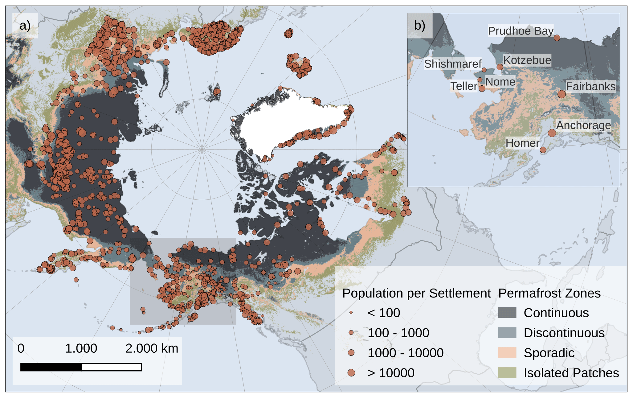
Figure 1 Panel (a) shows the pan-Arctic permafrost extent as modeled by Obu et al. (2019) together with the population numbers of settlements in the Arctic Circumpolar Permafrost Region (ACPR) (Wang et al., 2021). The different sizes of the circles represent logarithmic scaling of the population numbers. Our study focuses on the state of Alaska as shown in the inset map (b). The basemap was made with Natural Earth. Free vector and raster map data at http://www.naturalearthdata.com (last access: 14 August 2023).

Therefore, substantial efforts are being made to map settlements, areas of human activity and industrial sites throughout the Arctic. Extensive databases have been compiled regarding population numbers (Wang et al., 2021; Ramage et al., 2021), the occurrence and development of infrastructure along coastlines (Bartsch et al., 2020, 2021), and the distribution of industrial sites in the Arctic (Langer et al., 2023). The datasets focusing on Arctic infrastructure in particular and areas of human activities in general, however, are limited in spatial coverage (coastal areas, north of the treeline e.g., Bartsch et al., 2021; Xu et al., 2022) and spatial resolution and lack specific details regarding usage type. Furthermore, because of their diverse research approaches, these datasets are inconsistent with respect to spatial references and geometry types (vector or raster). To date, there has been no comprehensive inventory that synthesizes various data about infrastructure and areas of human activity in the Arctic and that combines this information with essential environmental data such as permafrost occurrence and watersheds. In addition, for Canada and the US there is a substantial volume available of state and federal data on contaminated sites (Langer et al., 2023). However, the geospatial data provided by government agencies are highly heterogeneous, offering the full range from detailed site chronologies (e.g., affected containment structures, mandated cleanup measures) as well as data about the polluting substances to sometimes only basic information about location, cleanup status and responsible personnel. Additional details can then be found in written reports (Langer et al., 2023; State of Alaska Department of Environmental Conservation, 2023a), and each detail has to be extracted first before it can be put into a spatial context. However, this detailed information is urgently required in a geospatial data format over large regions, not only to estimate the vulnerability of critical infrastructure and human-affected areas to permafrost degradation, but also to assess the ecological consequences of contamination resulting from industrial infrastructure site failures.

Focusing on Alaska, we thus (i) harmonized existing multisource data on infrastructure and human-impacted areas into a coherent usage type classification scheme; (ii) created a statewide inventory of these elements and enriched it with data on permafrost characteristics (extent, probability and ground temperatures), watersheds and sites of contamination, for which we extracted information on contaminants, cleanup duration and the affected medium from available text reports; and (iii) enabled the spatial analysis and queries of the inventory together with the ecological information in a database-like structure.

Following the CIIP manual (Critical Information Infrastructure Protection, CIIP2008) (Brunner and Suter, 2008), we define critical infrastructure as those sectors essential for the reliable functioning of communities. These core categories include among others food and water supply as well as health and sanitation. To better align with the modern and traditional ways of life in the Arctic and sub-Arctic regions, we have adjusted the internationally recognized core categories and extended them. Please refer to Sect. 2.2.1 (“infrastructure usage types”) and Table 1 for a full list of the categories.

2 Materials and methods

2.1 Study site

Alaska is the largest and northernmost state of the United States of America (US). With a population of over 733 000 inhabitants and a land area of approximately 1.7 × 10⁶ km² (The Information Architects of Encyclopaedia Britannica, 2023), it is also the least densely populated state in the US, with a population density of 0.5 people per square kilometer (1.3 people per square mile), compared to the rest of the US with a density of 35.9 people per square kilometer (93 people per square mile) (Department of Labor and Workforce Development, 2020; World Bank, 2024). Alaska is home to over 300 communities, with Anchorage, Juneau and Fairbanks being the biggest municipalities, housing 49 % of the overall population. Nearly half of the rest of the population (44 %) resides in smaller settlements with fewer than 10 000 people (Department of Labor and Workforce Development, 2020) dispersed across the entire state. Many of these smaller settlements are only reachable by air or barge (Hamilton et al., 2016).

Alaska encompasses a range of different landscapes, from glaciers in the Brooks Range to tundra in the North Slope and boreal forests in the Alaska–Yukon region (Raynolds et al., 2019; Jorgensen and Meidlinger, 2015). There are also substantial variations in meteorological and permafrost characteristics, following a north–south gradient. In the north, a cold polar tundra climate (Beck et al., 2018) prevails, with a mean annual air temperature (MAAT) of −10.4 °C (Climate Normals 1991–2010 of Deadhorse; see National Oceanic and Atmospheric Administration, National Centers for Environmental Information, 2023a) and a continuous permafrost extent (see Fig. 1). The south, on the other hand, is still characterized by a cold climate (Beck et al., 2018) but with much higher temperatures (4.5 °C MAAT for Homer; see National Oceanic and Atmospheric Administration, National Centers for Environmental Information, 2023b) and a permafrost extent transitioning to a sporadically underlain land surface and isolated patches.

It is important to note that approximately 80 % of the state's area – accounting for nearly 200 settlements (refer to Fig. 1) – falls within the permafrost region (Jorgenson et al., 2008; Ramage et al., 2021), which is projected to undergo massive changes in the upcoming decades (Chadburn et al., 2017; McGuire et al., 2018). Challenges such as ground subsidence across the region and coastal erosion along the extensive and populated coastline (occupied by 83 % of the population; NOAA Office for Coastal Management, 2023) will pose a high risk to the Alaskan population and economy (Melvin et al., 2016; Liew et al., 2022; Wang et al., 2023).

The most important contributions to Alaska's economy stem from the mining, quarrying, and oil and gas extraction industries (Bureau of Economic Analysis, 2023a). Notably, the oil exploration units in the North Slope and Cook Inlet play a vital role in Alaska's revenue, having contributed 38 % of the general funds in the 2019 fiscal year (Alaska Oil and Gas Association, 2020, 2021). In addition to the significant impact of oil and gas, Alaska's fishing industry plays a crucial role in the economy. The Alaska Seafood Marketing Institute (Alaska Seafood Marketing Institute, 2024) reports that, in 2021/22, the fishing industry employed 17 000 Alaskans (from a total of 48 000 workers) from more than 142 communities, making it the top employer in the Alaskan manufacturing sector. Moreover, more than 60 % of the total US seafood harvest comes from Alaska's fisheries (Alaska Seafood Marketing Institute, 2024). Further industries contributing to the economy are transportation and warehousing (including cargo and passengers but also tourism), finance, insurance, real estate, and government and government enterprises (including community services, e.g., military or postal services) (Bureau of Economic Analysis, 2023a, b). However, the economic growth comes with environmental consequences. The continued development of infrastructure, the expansion of human-impacted areas and oil exploration sites in the north as well as the associated transportation and infrastructure networks have already led to an increase in thermokarst occurrence (Raynolds et al., 2014; Walker et al., 2022). Furthermore, given the extensive oil and gas production operations, there is an inherent risk of environmental contamination resulting from infrastructure failures. This, in conjunction with both natural and human-induced degradation processes, underscores the need for a comprehensive and freely accessible database encompassing critical infrastructure and human-impacted areas on the one hand and environmental information concerning watersheds and permafrost on the other.

2.2 Data harmonization and mining

The SIRIUS (Synthesized Inventory of CRitical Infrastructure and HUman-Impacted Areas in AlasSka) dataset synthesizes data from five different sources:

1. the Sentinel-1/2-derived Arctic Coastal Human Impact dataset (SACHI) (Bartsch et al., 2021) (acquired on 11 June 2021);

2. the OpenStreetMap dataset for the infrastructure and land use information (OpenStreetMap Contributors and Geofabrik GmbH, 2018) (acquired on 20 January 2023);

3. the pan-Arctic Catchment Database (ARCADE) for the watersheds (Speetjens et al., 2023) (acquired on 17 January 2023);

4. the modeled Northern Hemisphere permafrost map by Obu et al. (2018) (acquired on 31 August 2023); and

5. the Contaminated Sites Database and reports by the State of Alaska Department of Environmental Conservation (2023a) (DEC) (acquired on 2 March 2023).

The primary task was to harmonize them to create a semantically and geometrically coherent and uniform data product (see Fig. 2). Initially, a thorough homogenization of the spatial reference was required. All the datasets were reprojected to the World Geodetic System 1984 with an Alaskan polar stereographic map projection (EPSG Code 5936). Subsequently, we clipped every dataset's spatial extent to the state boundary of Alaska as provided by the National Weather Service (2023). Each dataset had to undergo further geometric harmonization processes, e.g., merging individual vector files, creating buffer zones along linear features and clipping to layer spatial extents. Thereafter, we performed spatial analyses such as spatial overlays and joins to determine overlapping features and to retrieve their information. All data processing was done using Python with its geospatial data processing libraries geopandas, pandas, numpy, gdal, rasterio and rioxarray (Jordahl et al., 2022; pandas development team, 2023; Harris et al., 2020; Rouault et al., 2023; Gillies et al., 2013; Rio, 2024). The data processing scripts are downloadable from our Zenodo repository at https://doi.org/10.5281/zenodo.8311243 (Kaiser et al., 2023).

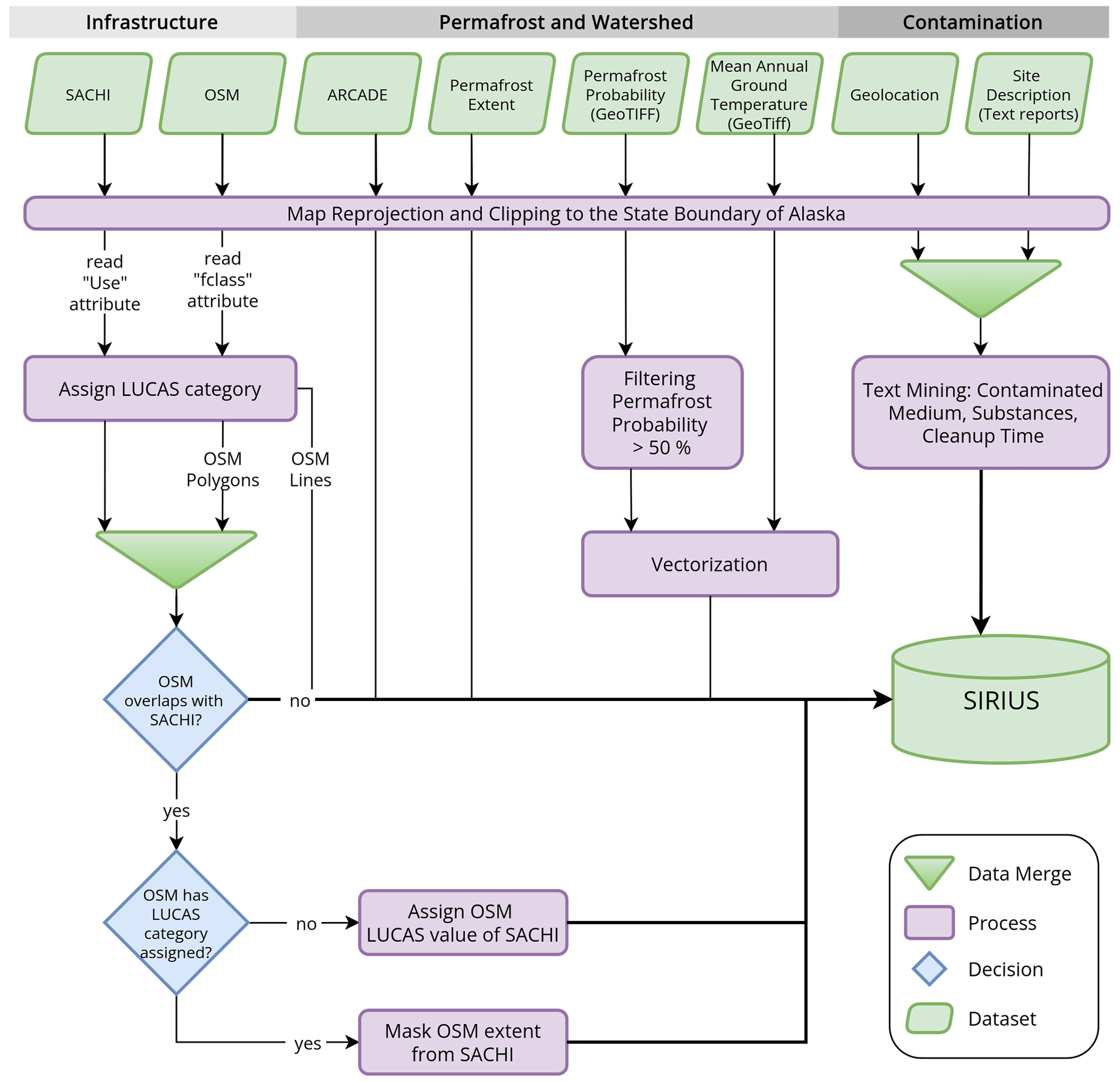
Figure 2 Flowchart of the harmonization process. If not indicated otherwise, all the input datasets have an ESRI Shapefile format.

2.2.1 Infrastructure and human-impacted areas

SACHI

The SACHI dataset contains buildings, road and railway networks, and other human-impacted areas in the Arctic coastal regions up to 100 km inland (Bartsch et al., 2020). The infrastructure features in SACHI were derived from Sentinel satellite imagery using machine learning and were blended with auxiliary information from other datasets (Bartsch et al., 2021). Each infrastructure feature has among other things information on the settlement name, the feature's class, the primary economic activity (attribute “use”) and the general economic activity (attribute “use main”) (Bartsch et al., 2021). The value of the attribute “settlement name” was assigned on the basis of the settlement dataset by Wang et al. (2021), with a 40 km buffer applied to also incorporate the surrounding infrastructure. Features outside this buffer were labeled following the Google hybrid data layer (Bartsch et al., 2021). Each settlement (and surrounding area) was then assigned one economic activity category. This procedure resulted in a rather coarse definition of use categories. For example, the settlement of Nome is assigned the general use category “mining”, with no further distinction, and for the Nome–Teller highway connecting the settlements of Nome and Teller the southern part (Nome) is assigned “mining”, while the northern part contributes towards the “fishing” industry in Teller. This generalization does not allow the differentiation of use categories within settlements and beyond. As the SACHI dataset was derived using a pixel-based approach, linear infrastructure is also represented as polygons. The “class” attribute specifies whether a feature corresponds to linear transport infrastructure (class =1), a building (class =2) or another human-impacted area (class =3). When we visually examined the linear transport infrastructure, we observed some gaps in the data, particularly in the settlements: extracting narrow paths or distinguishing between a linear gravel road and other human-impacted areas, such as driveways or exploration pads, was difficult with the limited spatial resolution of the Sentinel sensors (10 m). In addition, the “road” class showed a particularly low mapping accuracy compared to the “building” class (Bartsch et al., 2021). As OpenStreetMap (OSM) on the other hand is estimated to represent 83 % of the global road network (Barrington-Leigh and Millard-Ball, 2017; Hjort et al., 2018), we decided to use OpenStreetMap data to represent the linear transport infrastructure.

OpenStreetMap

The OSM project is a collaborative initiative involving mappers from around the globe, aiming to provide highly detailed and comprehensive map data (OpenStreetMap Foundation, 2023). It offers a wide range of geographic features, encompassing various categories such as settlement types (e.g., cities, hamlets, villages), road classifications (e.g., motorways, footways, primary and secondary roads), railway networks, amenities, human structures and more (OpenStreetMap Wiki, 2023). Notably, the road and railway networks in OSM are represented as line features. This trait facilitates queries about the total length of the road network sections situated on different types of permafrost or within specific catchment areas as well as the identification of potential contamination along the transportation routes. Another advantage of OSM is its data availability for the entire region of Alaska. Our focus is on areas (farmland, commercial areas, etc.) and elements (small-scale features, e.g., hunting stands or memorials) that are directly influenced by human activities and that are shaped by practical land use. Therefore, we excluded OSM files which contained information about water bodies and natural features: “waterways” for the linear infrastructure files and “natural” and “water” for the polygonal and point infrastructure files. We also excluded information on the orientation (Buddhist, Jewish, etc.) of religious sites: “pofw” (places of worship). Buildings such as churches, chapels and burial grounds (cemeteries) were retained. Subsequently, we merged the linear OSM infrastructure files into one dataset. To assess how the linear OSM infrastructure dataset compares to the pixel-based SACHI dataset, we compared their polygonal representations. For this, we converted the linear OSM infrastructure to polygons by applying a buffer around each linear feature: major highways and roads (OpenStreetMap Wiki, 2023) were assigned a width of 20 m to account for possible embankments, slip roads or ramps. For the rest of the road network and the railway lines, we assumed a width of 10 m. Subsequently, we clipped the polygonal OSM dataset – representing the linear infrastructure features – to the spatial extent of the SACHI dataset and compared their respective areas to each other.

After merging the linear railway and road network OSM data, we combined the polygonal OSM infrastructure data into a single GeoDataFrame. The attribute “fclass” of the polygonal OSM GeoDataFrame contains the tag, which people use to describe the mapped feature. In the OSM Wiki (OpenStreetMap Wiki, 2023), these tags are listed following a certain key and value combination, a mapping standard most members of the community follow. As a first step, we derived the unique values of fclass and compared them to the OSM values defined in the Wiki (OpenStreetMap Wiki, 2023). Generally, the tags under fclass were in agreement with the OSM values of the Wiki. Some mismatches originated from different expressions, e.g., “town_hall” instead of “townhall”, “archaeological” instead of “archaeological_site” or “mobile_phone_shop” instead of “mobile_phone”. Some tags were unofficial additions created individually by the OSM community, e.g., “parking_multistorey” or “recycling_paper”. Further, we removed any tags describing natural features (waterfalls, etc.) and places (island, heath, village, etc.), which portray localities and their population in which multiple usage types are possible. Table  shows the retrieved values of fclass and their corresponding OSM keys and values, which we assigned manually following the abovementioned Wiki. The predominant tag under fclass was “building”. This tag represented 81 % of the polygonal OSM dataset. To determine the usage type for these buildings, we analyzed their attribute “osm_type” of the dataset and once again compared the tags under osm_type to the OSM keys and values of the OSM Wiki. Having identified all of the tags under fclass and osm_type and assigned them an OSM key and value, we had gathered information on the features' main usage and purpose and could put them into usage categories.

Infrastructure usage types

For this, we followed the Land Use/Cover Area frame statistical Survey (LUCAS) of Eurostat (E4.LUCAS (ESTAT), 2018), which provides a framework for a consistent classification and harmonization of land use and land cover data (see Table 1).

Table 1 LUCAS categories with their respective sectors critical to the Arctic and sub-Arctic communities.

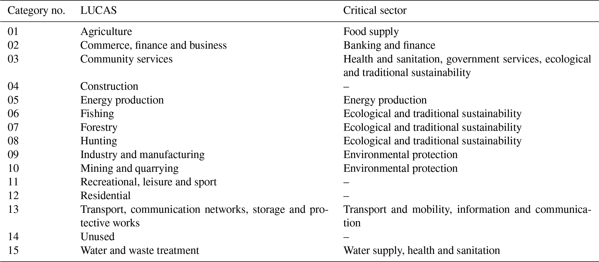
This categorization allows us to incorporate the aspect of sectors critical to the functioning of Arctic communities. Our core categories of critical infrastructure align with internationally defined sectors (Brunner and Suter, 2008), which include food and water supply, banking and finance, government services and institutions, transport and mobility, information and communication, energy production, and health and sanitation. In addition, we introduce two supplementary categories: ecological and traditional sustainability and environmental protection. The latter category refers to any infrastructure that may pose environmental hazards in the event of failure. This category is particularly significant for traditional lifestyles, such as hunting and fishing, which we consider to fall into the ecological and traditional sustainability category, as they rely on intact terrestrial and aquatic ecosystems. In this category, we also include sites of cultural heritage (cemeteries, tents, yerts, etc.; see, e.g., Irrgang et al., 2019).

Table  shows the assigned LUCAS category for each OSM tag. As the linear OSM data only consist of railway and road network data, no further classification was needed.

After implementing the initial assignment based on the given scheme, we noticed that all of the tags under fclass were effectively categorized, except for one: the “building” tag posed a challenge as the corresponding osm_type attribute lacked detailed information on the usage type for 86 % of the 144 000 building features. To address this, we subsampled the features with the fclass building that had not been assigned a usage type yet and “internally” overlaid them with features of any other fclass (other than building) that already had a usage type assigned. We then assigned the usage type of the non-building feature to the building feature in the overlapping areas. This analysis revealed that features with the tag “building” (e.g., a shopping mall) frequently contain various smaller features and, thus, usage types, such as shops, offices, parking areas and more. To harmonize this, we aggregated these diverse usage types and assigned the predominant usage type.

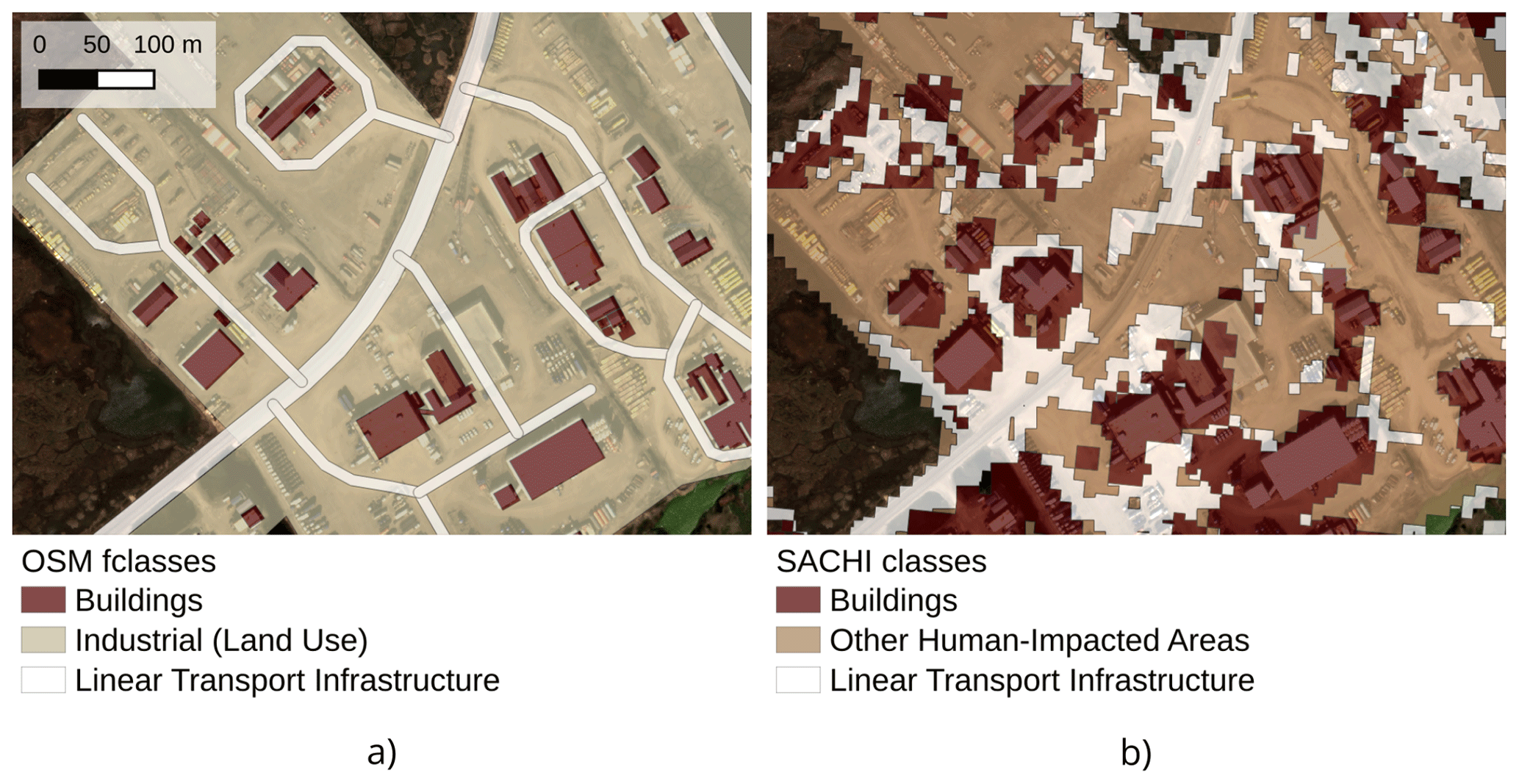
Figure 3 Comparison of the level of detail of the original (a) OSM and (b) SACHI datasets. OSM shows greater detail in mapping buildings, land use boundaries and linear transport infrastructure, in contrast to SACHI, where the delineation is done with a pixel-based classifier (Bartsch et al., 2021). The background RGB high-resolution imagery of Deadhorse is from WorldView-3 (copyright: DigitalGlobe, 2016). OSM data copyrighted by © OpenStreetMap contributors 2023. Distributed under the Open Data Commons Open Database License (ODbL) v1.0.

We processed the point OSM infrastructure data files in the same way: generating one GeoDataFrame containing all point features and assigning them a LUCAS category based on their tag under fclass. Eventually, we repeated the LUCAS category assignment for the SACHI dataset: each usage value was assigned a LUCAS category (see Table A2).

Combining SACHI and OSM

When visually examining subsets of the SACHI and OSM datasets, we again observed that the OSM data had a higher level of detail. The building boundaries of the OSM dataset were delineated accurately (see Fig. 3a), while the building outlines of the SACHI dataset were coarse and contained adjacent non-building areas due to the pixel-based approach (Fig. 3b). However, the SACHI approach detected more building areas. Therefore, we implemented a decision tree structure for the last harmonization step of the infrastructure and usage type datasets. As a first step, we retrieved all overlapping features of the OSM and SACHI datasets with a spatial join (see Fig. 2). When the OSM feature already had a LUCAS category assigned, we stored it in the final infrastructure and usage type dataset. If not, we assigned it the LUCAS category of the overlapping SACHI feature. All other non-overlapping SACHI and OSM features were also stored in the final infrastructure and usage type dataset.

2.2.2 Accuracy assessment

To assess and quantify the accuracy of our data integration of infrastructure and human-impacted areas, we subsampled an area of 0.3 km² of the coastal settlement of Shishmaref, for which very high-resolution imagery was available. We built a reference dataset by manually digitizing all presumably permanent infrastructure elements using multispectral (RGB + NIR) orthophotos with a spatial resolution of 10 cm acquired in 2021 with the Modular Aerial Camera System (MACS) by Rettelbach et al. (2023). Buildings and other polygonal infrastructure features, such as re-purposed shipping containers, small sheds and coastal protection structures, were mapped at a scale of 1:500. An infrastructure feature was considered permanent when it exhibited characteristics indicating a fixed location, such as supply pipes for shipping containers or fixed roofing. Roads were mapped at a scale of 1:2500 and solely if they exhibited an approximate width of 10 m or more to comply with the spatial resolution of the Sentinel sensors of SACHI. Subsequently, we created a grid layer spanning the mapped area with a size of 10 m by 10 m for each grid cell. Each grid cell was assigned the corresponding values of the (i) reference dataset and (ii) the SIRIUS infrastructure and human-impacted area dataset: the OSM keys and values, fclass, and the binary information if an infrastructure feature intersected the grid cell (yes or no). This allowed the calculation of a confusion matrix for the linear and polygonal infrastructures to determine the performance of the SIRIUS dataset.

In a confusion matrix, the classified dataset – in our case the SIRIUS infrastructure and human-impacted area dataset – is compared with the reference dataset to determine the performance of the classification (Maxwell et al., 2021). The matrix provides information on correctly classified pixels (with true positives, a “true” infrastructure feature of the reference dataset is also represented in the SIRIUS inventory; with true negatives, a grid cell of the reference dataset does not show an infrastructure feature, and nor does the SIRIUS inventory) and misclassifications (false positives and false negatives). A common metric derived from a confusion matrix is the overall accuracy (OA), the ratio of correctly classified pixels (true positive and true negative) to the total number of pixels (true or false) (Albertini et al., 2022).

2.2.3 Contaminated sites of Alaska

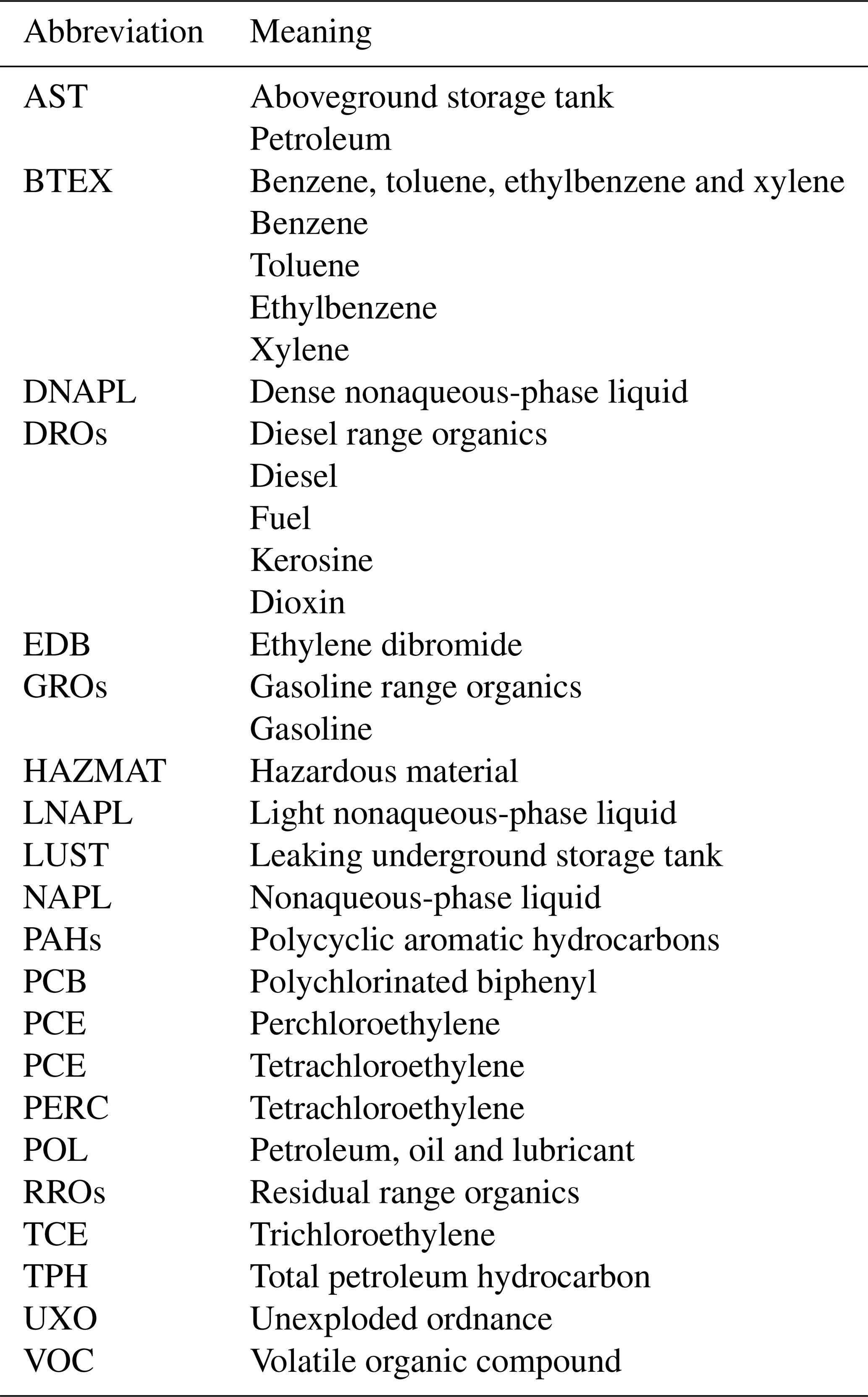
The Contaminated Sites Program (CSP) of the Alaska DEC provides statewide information about the contamination by hazardous substances and manages their cleanup (State of Alaska Department of Environmental Conservation, 2023a). The DEC dataset contains information on the site name, address, geographic coordinates, cleanup status, responsible staff, contact person and URL to a detailed site report. This site report contains complementary information on the contaminated medium (soil, groundwater, etc.), the substances (diesel, petroleum, etc.), and the date and type of cleanup measurements. We downloaded the detailed site report for each location to provide a harmonized dataset on contamination, infrastructure and human-impacted areas, which allows users to assess their interrelation with permafrost degradation and hydrological watersheds in Alaska. With basic text-mining tasks (regular expressions, filtering for uppercase words, etc.), we first derived all the abbreviations of the site report. We compared the abbreviations to the DEC's glossary (State of Alaska Department of Environmental Conservation, 2023b) and saved the ones indicating a substance or containment structure associated with contamination (e.g., LUST – leaking underground storage tank; PCBs – polychlorinated biphenyls) as a new attribute, “contaminants”, of the dataset. Subsequently, we made the dates followed by the expressions “site added to database”, “site closure approved” or “cleanup complete” (after 2008, State of Alaska Department of Environmental Conservation, 2023c) the start and end dates of the cleanup and saved them to the attributes “first_date” and “last_date”, which allowed us to calculate the total cleanup time (attribute “cleanup_days”). If these expressions did not appear in the site chronology report, we assumed the first and last mentioned dates to be the start and finish of the cleanup. From this, we calculated the total cleanup time in days and saved it as an additional attribute. These simple text-mining analyses were sufficient for deriving dates and uppercase abbreviations as well as for comparing our list of toxic substances and containment-related keywords to the full-text reports. However, we also wanted to provide information on the predominantly contaminated medium, i.e., whether the groundwater, soil or adjacent waterbodies were impacted. Here, we had to deal with high heterogeneity in the structure of each report. Some reports listed the contaminated medium under the section “contaminant information”. By comparing a set of medium keywords (soil, groundwater, river, etc.) with this section, we retrieved the contaminated media.

2.2.4 Permafrost data

As described for the infrastructure and contamination datasets, we assigned the joint spatial reference to the permafrost datasets and clipped their extent to the state boundary of Alaska. We derived the permafrost information from the modeled Northern Hemisphere permafrost map for 2000–2016 of Obu et al. (2018). The dataset is comprised of three GeoTIFF raster files containing the mean annual ground temperature (MAGT), the MAGT standard deviation, the permafrost probability fraction and one vector file (ESRI Shapefile) with information on the permafrost extent. The dataset is an estimation based on the TTOP (temperature at the top of permafrost) model, which uses the MAATs to model the MAGTs and subsequently the permafrost probability and zonation (Obu et al., 2019). It has a resolution of 1 km² and was validated by borehole data (Obu et al., 2019). Within our study, we integrated the data on a permafrost probability fraction and filtered for raster values where the probability of permafrost occurrence was greater than 50 %, complying with the definition of the permafrost model domain (Langer et al., 2023). The filtering step provides users with an additional filtering option for relevant permafrost information, as it allows the integration of mean annual ground temperatures. Subsequently, we vectorized the raster data to ensure compatibility with the other vector datasets. Given that each pixel value in the MAGT raster file was provided with a precision of up to five decimal places, our initial step involved rounding these values to a single decimal place before proceeding with the vectorization process. We also included the vector data on the permafrost extent (zones) to allow the user to query data dependent on the permafrost zone, e.g., continuous or sporadic.

2.2.5 ARCADE watershed database

The pan-Arctic Catchment Database, referred to as ARCADE, comprises a comprehensive collection of over 40 000 catchments draining into the Arctic Ocean down to a Strahler order of 5 (Speetjens et al., 2023). The geometries of the watersheds were derived from the Copernicus Digital Elevation Model with a spatial resolution of 30 arcsec (approximately 1 km). Additional information regarding the catchment characteristics (elevation, slope, etc.), climatology (precipitation, snowfall, runoff, etc.) and physiography (soil characteristics, permafrost parameters and extent, land surface data, etc.) has already been incorporated to enrich the dataset (Speetjens et al., 2023). However, the permafrost extent and information on the MAGTs were averaged over the extents of all the watersheds, which reach sizes of up to 3.1×10⁶ km² (Speetjens et al., 2023). Therefore, we chose to include the information on every 1 km² grid cell of the permafrost MAGT dataset of Obu et al. (2019) (see Sect. 2.2.4).

2.3 Data usability

To enhance spatial queries involving different usage types, contaminated sites, watersheds and permafrost information, it was necessary to consolidate the individual preprocessed files into a single container. For this, we chose the GeoPackage format as specified by the Open Geospatial Consortium (OGC). The GeoPackage format facilitates the exchange of geospatial data across different platforms, is open-source (Open Geospatial Consortium, 2023) and eliminates the need to handle multi-file data formats like ESRI Shapefiles. Thus, it is highly suitable for accommodating the diverse data-handling preferences of potential users. As GeoPackage uses a SQLite database container, the user is able to conduct their analyses within established geographic information systems such as ArcGIS, QGIS or spatial databases (Geopackage Contributors, 2020; GDAL/OGR contributors, 2023).

3 Results

3.1 Data harmonization and mining

In this section, we outline the enhancements made to the infrastructure and human-impacted area dataset of Alaska as well as the information on contaminated sites. To showcase the advancements achieved by combining the SACHI and OSM data, we focused on two coastal regions, Nome and Prudhoe Bay, by subsampling their respective datasets. Furthermore, we investigated the performance of simple text-mining tasks for the contaminated sites. For this, we randomly selected 10 sites from the dataset and verified the accuracy of the derived start and end dates, cleanup duration, and information regarding the substances and the contaminated medium. Subsequently, we analyzed in which cases the simple text-mining approach performed well and identified its limitations in other instances.

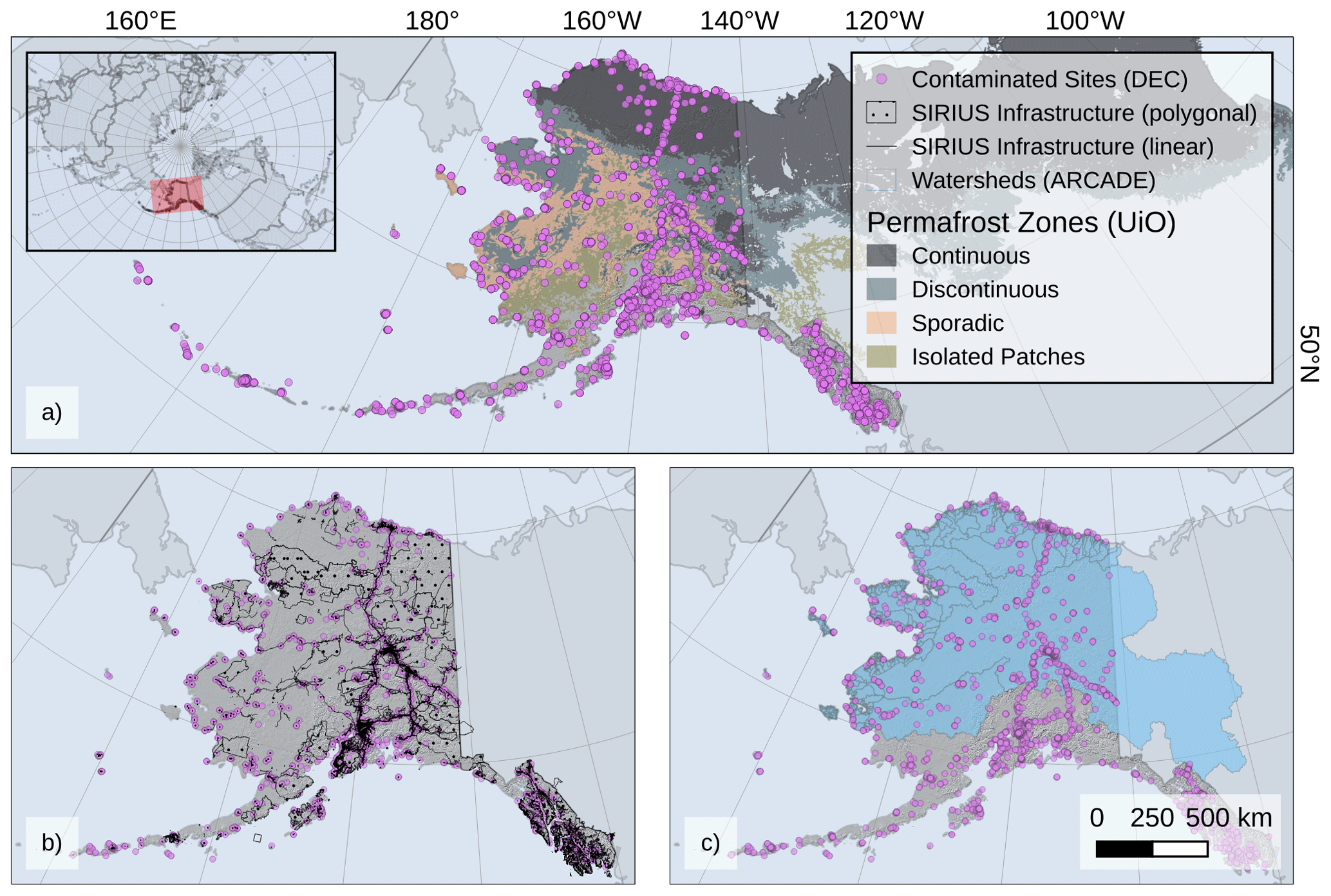
Figure 4 Overview of the synthesized data: contaminated sites and (a) modeled permafrost zones, (b) combined SACHI and OSM infrastructure and human-impacted areas, and (c) watersheds draining into the Arctic Ocean and the Bering Sea. OSM data copyrighted by © OpenStreetMap contributors 2023. Distributed under ODbL v1.0. The basemap was made with Natural Earth. Free vector and raster map data at http://www.naturalearthdata.com (last access: 14 August 2023).

3.1.1 Infrastructure and human-impacted areas

The data fusion of the OSM and SACHI datasets resulted in an infrastructure and human-impacted area map with higher spatial detail and coverage than the original datasets. While the polygonal features of SACHI only covered the coastal region with an area of 62 km², the incorporation of OSM data extended the infrastructure map to encompass the entire state, now covering an expansive 640 593 km².

Furthermore, the integration allowed us to enhance the level of detail regarding the usage categories for various infrastructure features. While we were able to initially assign five LUCAS categories to the SACHI data, i.e., fishing; mining and quarrying; energy production; community services; and recreational, leisure and sport, the inclusion of OSM data expanded this categorization to include an additional eight categories: agriculture; commerce, finance and business; construction; forestry; industry and manufacturing; residential; transport and communication networks; and waste and water treatment (refer to Table A3 and Fig. 6 for a detailed breakdown).

This comprehensive categorization enhancement enabled us to refine the generalized approach. For example, we discovered that energy production sites, initially thought of as dominant with an area of 28 km² in coastal regions, were, in fact, less extensive, covering only 17 km² across the entire state (see Table A3 and Fig. 6).

However, by incorporating the SACHI dataset, the map now also encompasses small and isolated elements like gravel pads and small paths, which were not mapped by the OSM community but which were successfully derived from the satellites (refer to Sect. 2.2). On the other hand, the integration of OSM data provided a heightened level of detail, enabling clear identification and differentiation of roads and single buildings (see Fig. 5c).

Looking at the settlement of Nome using SACHI, we identified mining and quarrying as the primary land use category, apart from the transport network. These categories were determined by applying a buffer around each settlement (refer to Sect. 2.2.1) and assigning it one predominant value (see Fig. 5b). Combining SACHI with the OSM data enhanced the quality of the transport network, where the streets are clearly defined even within areas with a high density of buildings and other human-impacted areas. It also improved the detail of these usage type categories (Fig. 5c). We learned that the majority of the settlement's area is actually residential, characterized by houses and recreational areas such as pitches and parks (see Fig. 5a and c). The OSM data also added detail, where the spatial resolution of the SACHI product derived from Sentinel satellites fell short. For example, the pier in the western area was not captured by the Sentinel satellites, but it was digitized by the OSM community. However, comparing the resulting human-impacted areas and the infrastructure map with aerial imagery from Bing (as accessed via the QGIS plugin OpenLayers; Sourcepole AG, 2024) revealed that there is a second pier, which did not appear in OSM or in the SACHI dataset. Nonetheless, the true added value of the SACHI dataset is in its information on small features such as extraction pads and others, which only occasionally appear in OSM data.

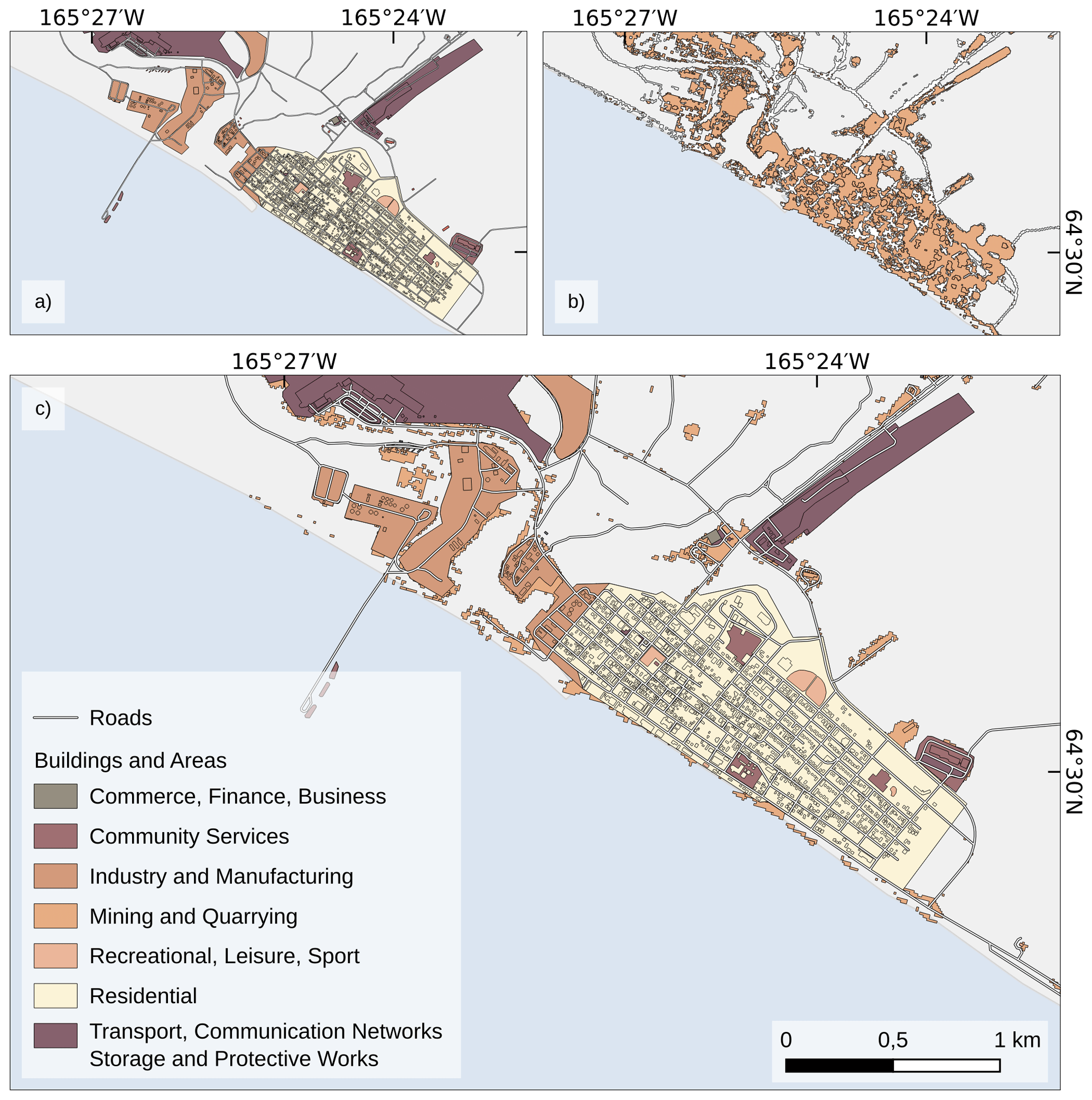
Figure 5 Input data from (a) OSM and (b) SACHI assigned to LUCAS categories for the example of the settlement of Nome located along the Bering Sea coast. Map (c) shows the harmonized data on the infrastructure and human-impacted areas of SIRIUS. OSM data copyrighted by © OpenStreetMap contributors 2023. Distributed under ODbL v1.0. The basemap was made with Natural Earth. Free vector and raster map data at http://www.naturalearthdata.com (last access: 14 August 2023).

A closer examination of the Prudhoe Bay area confirmed this observation. Once again, the SACHI dataset showed more human-impacted areas, probably from expanding exploration sites, while OSM offered more spatial detail. Furthermore, at both sites, we found that OSM exhibited higher quality in terms of linear infrastructure objects such as road and railway lines. As mentioned in Sect. 2.2, we compared the areas of the linear transport network between SACHI and OSM to evaluate the potential limitations of using OSM data. However, we discovered that the difference in area was only 5 km² (or 6 % of the total SACHI linear infrastructure area), as shown in Table A3.

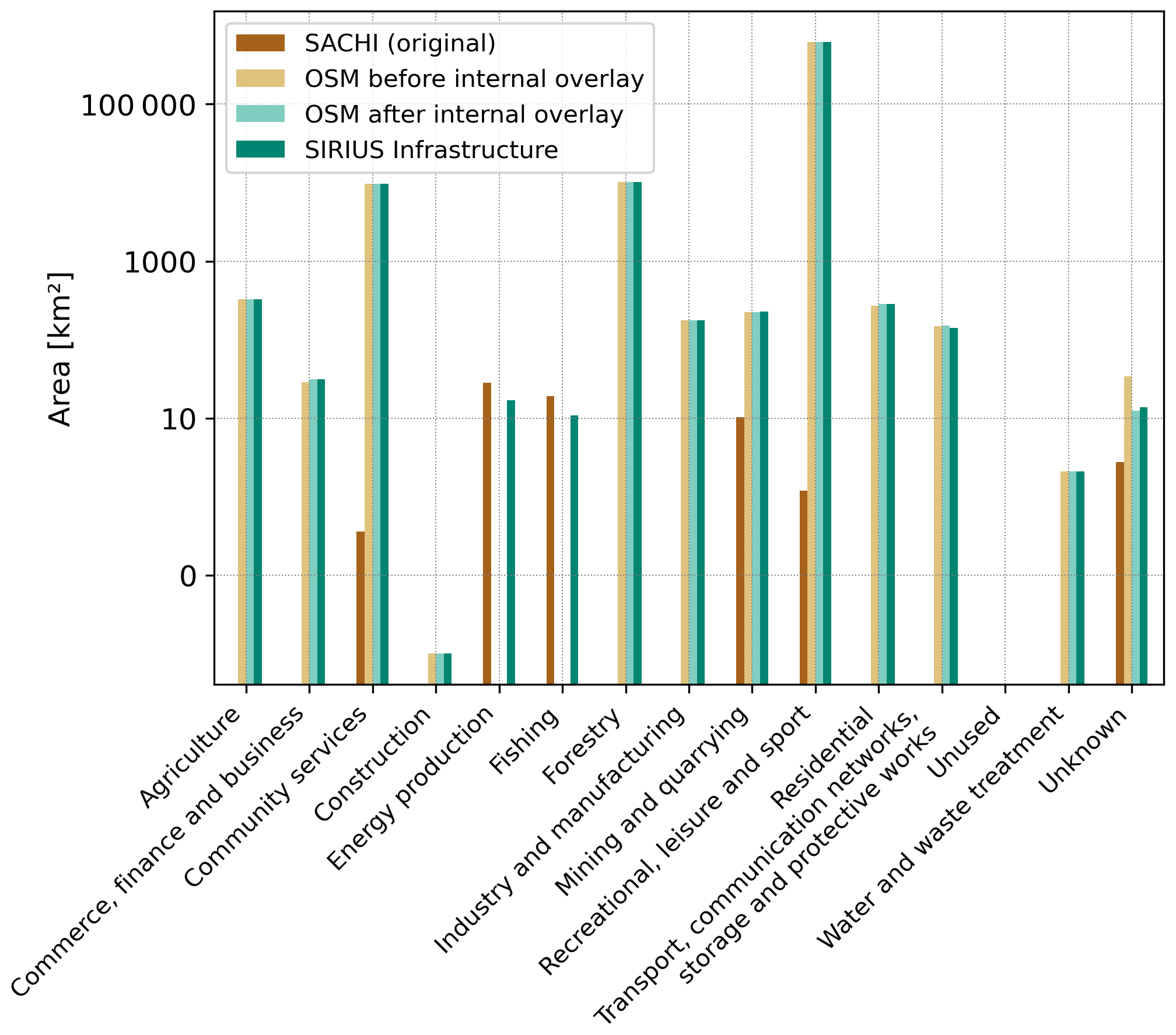
Figure 6 Improvement of the spatial coverage and usage type categorization. Area (km²) per LUCAS category for (i) the original SACHI dataset (only coastal areas), (ii) OSM before and (iii) after the internal overlay (complete extent of Alaska), and (iv) after combining both datasets within our SIRIUS inventory of infrastructure and human-impacted areas. For detailed values, refer to Table A3.

The resulting SIRIUS infrastructure and the human-impacted area inventory not only represents economic activities, but also incorporates fundamental functions for living (Maier et al., 1977), including agricultural areas, commercial and residential zones, recreational spaces, waste and water treatment, and community services. We also observed a significant decrease in the number of features with unknown land use types by internally overlaying OSM buildings with non-building OSM information (see Fig. 6 and Table A3). Prior to the internal overlay, the area with unknown land use was 34 km², whereas, after the overlay, it decreased to only 13 km² (refer to Table A3). This enhanced level of usage type detail allows for various applications, such as risk assessments for energy production facilities and transportation networks as well as evaluations of contaminated sites close to recreational or agricultural areas (refer to Sect. 3.2.1).

3.1.2 Accuracy assessment

The OA of the confusion matrix represents the ratio of correctly classified pixels to the total number of all pixels (positive and negative, true and false). The OA of the linear infrastructure data of SIRIUS is 0.5. While this value seems relatively low, we need to zoom in on a specific detail: of all 310 true road grid cells of the reference dataset showing a road infrastructure, 241 grid cells, i.e., 78 %, were accurately represented in the SIRIUS dataset (see Fig. 7a). A visual examination further revealed that, of the remaining 69 true road grid cells supposedly not represented by SIRIUS, 45 (65 %) were captured but with a slight spatial offset (see Fig. 8a), leading to a false negative when indeed it was only a positional inaccuracy. Taking into account these offset grid cells, the overall accuracy of the SIRIUS dataset improves to 0.69 and the true positive value increases from 0.78 to 0.92, indicating that 92 % of the road infrastructure is mapped in the SIRIUS inventory. All of the SIRIUS road grid cells not mapped in the reference dataset (false positives) were either small tracks, footways or narrow residential roads with widths of less than 10 m, and thus they were not mapped (see Fig. 8b).

The overall accuracy of the polygonal infrastructure and human-impacted areas of the SIRIUS dataset shows a similarly low value of 0.53. However, the true positive value, representing the ratio of the correctly classified values in SIRIUS to the actual positive values, is 94 % (686 of 731 true polygonal infrastructure grid cells) (Fig. 7b). Of the remaining 45 false negative grid cells, 13 % were indeed missing, another 18 % occurred again because of a spatial offset and 69 % appeared along the breakwater, protecting the shore (see Fig. 9a). OSM did not capture this structure, and due to the relatively coarse spatial resolution of the Sentinel sensors, the representation of the breakwater was sparse and patchy in SACHI, leading to an underestimation and a high number of false negatives.

However, substantially distorting the overall accuracy is the high number of false positives: 568 grid cells showed an intersection with the polygonal infrastructure in the SIRIUS dataset (Fig. 7b), which was not captured in the reference dataset; 23 % of these false positives stem from an overestimation of the airport area in SACHI and an altogether more generous mapping of the area in the OSM data. The eastern part of the runway, for instance, appears revegetated and allows the conclusion that it is no longer in use despite still being represented in the OSM data (refer to Fig. 9b). However, the highest number of false positives originates from areas affected by human activities represented in the SIRIUS dataset. These human-impacted areas posed a challenge to accurately mapping them for the reference dataset on the basis of the orthophotos alone. Some features, e.g., a playground, were either not visible or were difficult to delineate accurately. Figure 9c shows an example of a human-impacted area mapped as industrial land use by the OSM community. While the single storage structures are represented in the reference dataset, there was no indication of an enclosed area.

In summary, the low overall accuracy of the polygonal infrastructure data is distorted by a high number of false positives that originate from either an overestimation of the areas (e.g., airport) or a (conceptual) definition of land use (e.g., playground, industrial usage) that is difficult to reproduce with orthophotos alone. However, it is important to note that SIRIUS achieved representations of 78 % for the linear infrastructure and 94 % for the polygonal infrastructure, respectively, of the true infrastructure values.

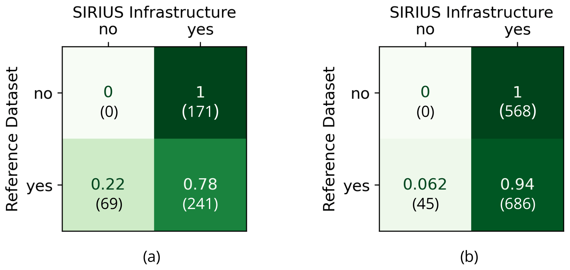
Figure 7 Confusion matrices were used to evaluate the accuracy of the SIRIUS dataset. The integrated SIRIUS inventory is compared with the reference data, which were mapped on the basis of orthophotos acquired in 2021. The matrices were normalized to the “true” value, representing the ratio of correctly and incorrectly SIRIUS-mapped features for each true class label (values [0–1]). Panel (a) shows the accuracy of the linear infrastructure features with a true positive value of 0.78 and a false negative value of 0.22. For the polygonal infrastructure, as seen in panel (b), the true positive value is 0.94, making the SIRIUS inventory highly thorough.

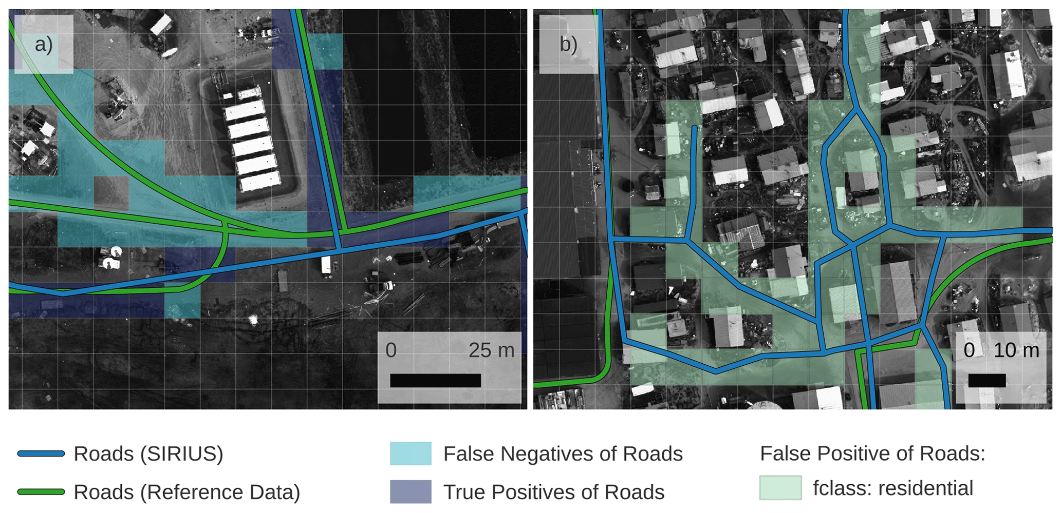
Figure 8 Comparison of the road network as represented in the SIRIUS inventory (integrated from OSM and SACHI from 2023 and 2021, respectively) and the reference data, which were mapped on the basis of multispectral (RGB + NIR) very high-resolution orthophotos from 2021. Panel (a) showcases the presumably false negative values (0.22) of the SIRIUS road network, revealing that the roads are indeed present but exhibit a slight offset. Panel (b) shows a section of the SIRIUS road network, which was deemed a false positive (1.0). However, the roads in SIRIUS are clearly visible in the imagery, yet they were not mapped due to their width being less than 10 m. Background imagery: orthophotos of Shishmaref used to build the reference dataset (Rettelbach et al., 2023).

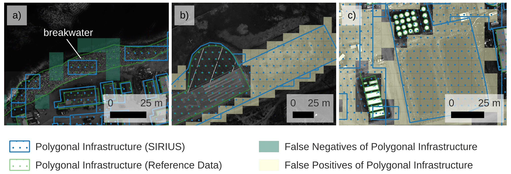
Figure 9 Comparison of the polygonal infrastructure and human-impacted areas as represented in the SIRIUS inventory (integrated from OSM and SACHI from 2023 and 2021, respectively) and the reference data, which were mapped on the basis of multispectral (RGB + NIR) very high-resolution orthophotos from 2021. Panel (a) shows a subset of false negatives (0.06 in total) along the breakwater as a consequence of the patchy representation of this feature in SACHI. Panel (b) displays the overestimation of the airport's runway in the SIRIUS dataset by including a revegetated area seemingly no longer in use. In panel (c), the area close to the storage features is represented as industrial land use in SIRIUS, which could not be identified on the basis of the orthophotos alone and is thus considered a false positive. Background imagery: orthophotos of Shishmaref used to build the reference dataset (Rettelbach et al., 2023).

3.1.3 Contaminated sites of Alaska

With the text-mining approach, we successfully extracted additional information from the site reports of the Contaminated Sites Program. The use of regular expressions allowed us to identify dates, abbreviations and references to substances from the DEC glossary or any contaminated medium mentioned in the text. Consequently, we were able to calculate the total cleanup time at inactive sites and provide a comprehensive list of the substances mentioned in the site reports. To assess the accuracy, we retrieved a sample of 10 data entries from the dataset (see Table A4). We confirm the successful extraction of dates, following the pattern described in Sect. 2.2.3. The expressions “sites added to database” and “sites closure approved/cleanup complete” were considered to be the first and last action dates, respectively. In the cases where no specific expressions were present, the first and last mentioned action dates were used instead. However, in 491 (6 %) entries, the cleanup duration was recorded as 0 d (for an example, see Hazard ID 2361 of the sample in Table A4), and in 214 (2 %) cases, negative values were even reported. This again points to a heterogeneous approach or methodology used by the agency to input data into the database. In these cases, “site closure approved/cleanup complete” was entered on the same date or even before “sites added to database”. For the sample, the retrieval of the contaminants was highly successful, as all substances and containment structures listed in the DEC glossary (see Table A5) were found. However, any substances not appearing in the glossary will not be retrieved with our approach. Also, the information regarding the contaminated medium was limited, as the DEC rarely provides details in the “contaminant information” section of the reports. Consequently, we were only able to derive the contaminated medium for 3321 (39 %) of the 8533 sites.

3.2 Data usability

The resulting GeoPackage with our preprocessed spatial data layers contains all the input data on watersheds, permafrost probability, zones and MAGT within the geographic extent of Alaska, projected to a joint spatial reference (EPSG code 5936). Additionally, it includes information on the contaminated sites, infrastructure features and other human-impacted areas. These datasets have undergone harmonization and enrichment, specifically focusing on the retrieval of the detailed land usage information and the types of contamination and the duration of cleanup measures, as outlined in Sect. 2.2.1 and 2.2.3. These datasets are now stored as separate layers (see Fig. A2), eliminating the need for managing multiple ESRI Shapefiles and their auxiliary files. While retaining their original fields such as ID, geometry or watershed names, the files have been enriched with new information recorded in additional fields.

We deployed two GeoPackages with the same data. However, in PermaRisk_RRNetworkLine.gpkg, the railway and road networks are represented as linear geometries and in PermaRisk_RRNetworkPolygonal.gpkg as polygonal geometries, based on the geometry buffers we defined in Sect. 2.2.1. This allows more detailed spatial queries, such as deriving the length of a road or railway line within a specific research domain (see Sect. 3.2.1). Considering the different user requirements, the GeoPackage can be imported into a spatially enabled database, such as PostgreSQL/PostGIS, loaded into a geographic information system (GIS), or used within geospatial processing libraries, such as Python's GeoPandas. In this section, we will showcase the use of our GeoPackage within QGIS, perform SQL queries and access it using GeoPandas to generate exemplary statistics and explore potential application scenarios.

3.2.1 Application

As a first application scenario, we wanted to retrieve the total length of the road and railway lines within Alaska's continuous permafrost zone. As GeoPackage uses an SQLite database container, we were easily able to query spatial information by using the “execute SQL” command in QGIS.

    SELECT SUM(ST_Length(RRnetwork.geom))
    FROM SACHI_OSM_InfrastructureHIElements_RRNetwork AS RRnetwork
    JOIN UiO_PermafrostZones AS permafrost
    ON ST_Intersects(RRnetwork.geom, permafrost.geom)
    WHERE permafrost.EXTENT = 'Cont';

This query provided us with a length of 8456 km for the railway and road networks intersecting the continuous permafrost zone.

Another possible application is to determine the number of contaminated sites per watershed. To achieve this, the user can for example use the QGIS tool “count points in polygon”. We tested this and discovered that the Yukon watershed, which is also Alaska's largest watershed draining into the Arctic Ocean, contained the highest number of contaminated sites, totaling 2256. However, to account for the huge differences in watershed sizes and to normalize the number of sites per area, we further calculated the number of contaminated sites per square kilometer per watershed, showing that the watersheds along the coast of the Beaufort Sea (Fig. 10a and c) and Kotzebue (Fig. 10b) depict the highest density of contaminated sites per square kilometer (see Fig. 10).

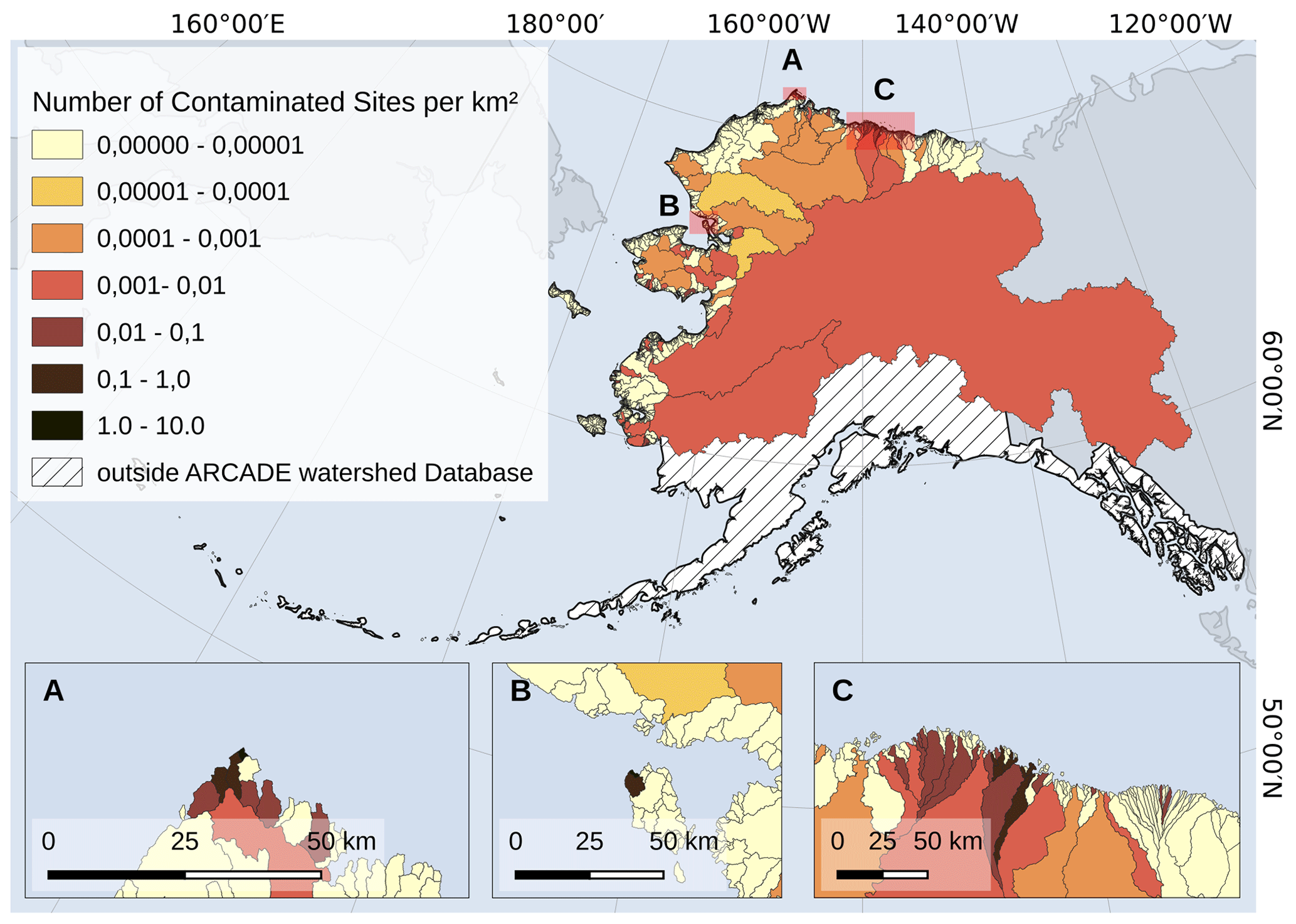
Figure 10 Number of contaminated sites per ARCADE watershed per square kilometer. The inset map (a) shows a watershed along the coast of the Beaufort Sea, with the highest value of 1.76 contaminated sites per square kilometer. Other watersheds exceeding more than one contamination per square kilometer were located in Kotzebue (inset map b) and on St. Lawrence Island. The inset map (c) shows a range of watersheds of the Prudhoe Bay area. The basemap was made with Natural Earth. Free vector and raster map data @ naturalearthdata.com at http://www.naturalearthdata.com (last access: 14 August 2023).

We further derived which land use category or infrastructure type shows the most contamination. For this analysis, we showcase the use of GeoPandas as a third processing option for our GeoPackage. By creating a spatial join between the SACHI_OSM_InfrastructureHIElements and SACHI_OSM_InfrastructureHIElements_RRNetwork (as a polygonal representation) layers along with DEC_ContaminatedSitesAK, we first derived all infrastructure and human-impacted areas and elements intersecting a contaminated site. Next, we dissolved these intersecting elements based on their LUCAS attribute. Subsequently, we counted the number of contaminated sites by examining the points within these dissolved polygons, representing the aggregated LUCAS attribute. For the Python code, see Appendix B.

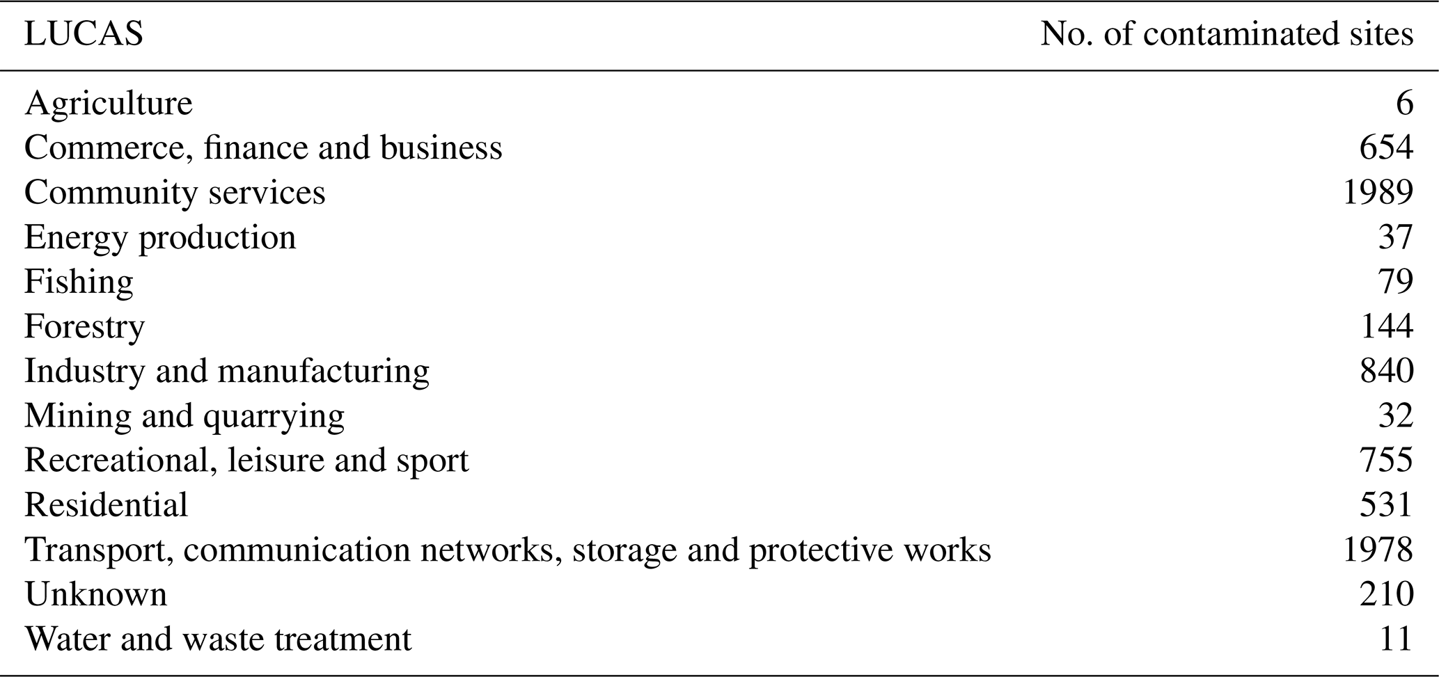
This application example showed that most of the contamination occurs in the land use categories “community services” (into which among others fall, e.g., military installations; see Table ), “transport, communication networks, storage and protective works”, “industry and manufacturing”, and “recreational, leisure and sport” (see Table 2).

Table 2 Number of contaminated sites per land use category.

4 Discussion

4.1 Data harmonization and mining

4.1.1 Infrastructure and human-impacted areas

The resulting inventory on infrastructure and human-impacted areas and elements in Alaska provides a detailed and comprehensive overview of various human activities, encompassing not only economic functions, but also fundamental functions for living. Compared to the original SACHI dataset, we have achieved higher spatial detail and coverage throughout the entire state by incorporating OSM data (see Table A3 and Fig. 6). On the other hand, the SACHI dataset has made a substantial contribution by capturing small elements that had been missed by the mapping efforts of the OSM community. This limitation may be attributed to the peripheral status of Arctic environments within the global OSM network, primarily due to their sparse population. Hjort et al. (2018) report such a limitation for isolated, smaller communities and with regional variability (e.g., better coverage in North America and Eurasia compared to Asia). This deficit in the mapped regions underscores the necessity for infrastructure products derived from remote sensing images, such as SACHI, as the underlying algorithms used to retrieve these features remain unbiased in terms of area selection. However, as described in Sect. 2.2.1, the algorithms fell short in densely populated areas, which makes distinguishing between adjacent features of different classes – e.g., buildings, roads or extraction pads – challenging. To achieve the spatial detail of the OSM additions, the retrieval of infrastructure and human-impacted features could be enhanced by analyzing remote sensing data with sub-meter spatial resolution. However, this improvement would come at a significant cost, as most of these satellite images are commercial. On a pan-Arctic scale, this approach is nearly impossible due to the large spatial coverage necessary and the associated high-resolution imagery costs (Manos et al., 2022). A compromise could involve using satellite imagery from providers that offer educational programs or discounted rates for researchers, such as Planet's Planetscope with a spatial resolution of 4 m (Sentinel Hub, 2024). Alternatively, deep-learning models could be leveraged to generate high-resolution images from lower-resolution sources like Sentinel-2 (Wang et al., 2018). Considering these challenges emphasizes the need to rely on crowd-sourced map data. These map data can also be generated remotely using accessible Web Map Servers or GIS plugins (e.g., Bing). Using OpenStreetMap as this data source serves as a gateway for this purpose. It establishes a low threshold for non-researchers, including citizen scientists, who can not only map various elements but can eventually also incorporate valuable information on contamination that has not been captured by official environmental agencies, highlighting the unique potential of OSM in this context. In addition, this approach allows the continuous development of suitable tags (the attribute fclass in our data). However, based on our own field visits, we have identified instances where certain areas and elements that contribute to the critical sector of “health and sanitation” are not accurately represented in OSM. For example, the Middle Salt Lagoon in Utqiaġvik (formerly Barrow), which is used for sewage purposes, is labeled “water” in OSM and is thus not included in our SIRIUS dataset. This underlines the need for a comprehensive review of the mapping tags before basing future inventories of critical infrastructure and human-impacted areas on OSM. Fortunately, due to OSM's open design and accessibility, these revisions can be easily implemented. Given that OSM undergoes daily updates through user contributions, the integration of OSM data also facilitates periodic updates within our inventory.

4.1.2 Accuracy assessment

While the linear infrastructure data exhibited low overall accuracy in our Shishmaref test area, about two-thirds of the false negatives resulted from a spatial offset (see Fig. 8). This indicates the presence of roads but with reduced positional accuracy, likely due to an image offset between the MACS imagery and the OSM data. All false positives were narrow residential roads or small paths visible in orthophotos but not digitized in the reference dataset, in order to comply with the 10 m Sentinel resolution. Including these narrow features in the reference dataset would have substantially improved the accuracy.

Nonetheless, 78 % of the true road grid cells were accurately represented in the SIRIUS dataset, increasing to 92 % when accounting for offset grid cells. This highlights the effectiveness of OSM in representing linear infrastructure compared to SACHI. OSM distinguishes between roads and adjacent infrastructure areas and includes narrow roads and footways. To improve the accuracy, it could be beneficial to integrate official data from local or federal agencies (e.g., the Alaska Department of Transportation) to evaluate the comprehensiveness of the OSM linear infrastructure data. Further, incorporating the Trans-Alaskan Pipeline would provide a spatial context for contamination, oil exploration and transportation data.

In the case of the polygonal infrastructure for the Shishmaref test area, the SIRIUS dataset achieves a representation of 94 % of all the true values. Distorting the overall accuracy are the false positives, approximately one-fourth of which belong to the area of Shishmaref's airport runway that is no longer in use. It is important to note that OSM encourages users to regularly update features. If a user finds that a feature no longer physically exists, they should delete it or tag it as “nonexistent” (OpenStreetMap Wiki, 2024b). If a feature still physically exists but is no longer in use, users are encouraged to tag it as “disused” (OpenStreetMap Wiki, 2024a). In this specific context, and considering the potentials of the contamination, it could be seen as an asset to have former land usage and industrial legacies represented in the SIRIUS dataset. An interesting approach might thus be to specifically filter for the OSM tags nonexistent and disused – in the regularly updated and historical OSM database – to highlight potential contamination sites.

The same applies to the human-impacted areas, such as playgrounds and industrial land use. While these features are important infrastructures critical to Arctic communities, they largely cannot be mapped on the basis of orthophotos alone. Accordingly, the polygonal infrastructure lacks this level of detail when derived from SACHI. As discussed in Sect. 4.1.1, the coarse spatial resolution of the Sentinel sensors poses a challenge in densely populated areas. In such regions, buildings and human-impacted areas become difficult to separate from adjacent roads. This challenge contributes to the high number of false positives, where roads are misclassified as buildings and areas of human activities are overestimated. However, this issue could be addressed using imagery with a higher spatial resolution.

It is important to note that the high mapping accuracies of 78 % (92 %) for the linear infrastructure and 94 % for the polygonal infrastructure in our test area of Shishmaref can likely be expected for most of the coastal regions (until 100 km inland). For inland areas (beyond the extent of SACHI), the infrastructure data rely solely on OSM, which may show the abovementioned limitations. Once again, integrating further official data sources could improve their quality.

4.1.3 Contaminated sites of Alaska

We were able to successfully enhance the DEC Contaminated Sites dataset with complementary information regarding the substances, the affected medium and the duration of the cleanup measurements. However, the text-mining approach, using regular expressions to compare site reports to the DEC glossary to retrieve the contaminant and the affected medium, encountered limitations where data were entered heterogeneously into the database (see Sect. 3.1.3). For instance, only 39 % of the site reports included information about the contaminated medium in the designated section “contaminant information”. In addition, in some cases, comparing the medium's keywords (soil, groundwater, etc.) to this section led to false positives as these terms are frequently used to describe the hazard level of the substances. The first entry (Hazard ID 26994) of our validation sample (refer to Table A4) is one of these false positives. The site report actually lists “soil” as a contaminated medium, but the level description for the substances “benzo[a]anthracene and benzo[a]pyrene” is “between method 2 migration to groundwater and human health/ingestion/inhalation”. Consequently, our approach also lists groundwater as a contaminated medium, which is not accurate. If we were to compare the full report to these keywords, this would result in even more incorrect classifications, as these terms are also employed to describe a suspicion of contamination. Furthermore, using regular expressions for the retrieval of the polluting substances does not differentiate between the presence and absence of a contaminant, e.g., “PCB was found” vs. “PCB was not found”. Although we did not encounter statements of absent contaminants in the reports of our sample, we cannot rule out the possibility of false positives of this kind.

These shortfalls could be addressed by implementing advanced text classification approaches from natural language processing and text mining. This could provide a more comprehensive understanding of toxic substances, including those not mentioned in the DEC glossary. Furthermore, these methods would extract and classify information on the contaminated medium from the entire report, rather than solely relying on the sampled section labeled “contaminant information”. Another viable alternative would be the integration of large language models (LLMs). We tested our particular false positive case (Hazard ID 26994) with the LLM chatbot ChatGPT Version 3.5 by copying the full report into the prompt and requesting “reading this text, tell me what medium (soil, groundwater, river, lake, etc.) was contaminated:”, and it correctly classified the affected medium:

Based on the provided text, the medium that was contaminated is `Soil'. The text mentions that soil samples collected during site assessment activities showed elevated concentrations of contaminants, specifically `benzo(a)pyrene' and `benzo(a)anthracene', which exceeded certain cleanup levels. Therefore, the contamination occurred in the soil medium.

In this way, inconsistencies in data entries and false classifications could be easily addressed.

4.2 Data usability

4.2.1 Application

All the resulting datasets have been organized as individual layers within a single GeoPackage, which is available for download from our Zenodo repository (see the “Code and data availability” section). The GeoPackage does not have to be extracted (e.g., like a .zip archive), nor does it rely on the handling of multi-file data formats such as ESRI Shapefiles. The user can seamlessly integrate it by either opening it in a GIS application or importing it into a spatially enabled database like PostgreSQL/PostGIS. In this way, each layer can be analyzed independently or in conjunction with the others, facilitating easy querying of critical infrastructure and human-impacted areas and their interrelation with environmental parameters.

To achieve a more comprehensive understanding of the socioeconomic implications of permafrost degradation, we advocate incorporating additional environmental data, such as soil and waterbody databases, which are important for assessing the contamination severity and the significance of waterbodies as water resources. Additionally, incorporating demographic factors like age distribution, education, employment and income numbers can provide valuable insights into the impacts of permafrost degradation on the population's wellbeing.

5 Code and data availability

The GeoPackage and Python codes are available from https://doi.org/10.5281/zenodo.8311243 (last access: 25 September 2023) (Kaiser et al., 2023).

6 Conclusions

The SIRIUS dataset offers a comprehensive inventory of critical infrastructure and human-impacted areas in Alaska. It enables researchers and local communities to explore data in a spatial context, providing valuable information on permafrost extent, permafrost probability, mean annual ground temperatures and watersheds, allowing for an in-depth analysis of their interdependencies.

By combining the OSM and SACHI datasets, the information content regarding the type of infrastructure usage was greatly improved, increasing the number of usage categories from 5 (in SACHI) to a total of 13. The new usage categories now go beyond industrial and other economically important infrastructure by distinguishing elements of healthcare, food and water supply, sanitation, and areas of cultural heritage that are crucial to the well-being of local communities. Leveraging the OSM data and internally overlaying building features with non-building features, we were also able to reduce the number of buildings with the unknown usage type by 63 % (from 34.15 to 12.58 km²).

As we move forward, we have identified several steps to enhance the SIRIUS dataset further. Future updates will incorporate the new version of the SACHI dataset, which was released during the review period of this paper. Version 2.0 encompasses (i) a refinement of the linear infrastructure features, now distinguishing between asphalt and gravel transport infrastructures; (ii) airstrips; (iii) human-influenced waterbodies and reservoirs; and (iv) additional regions further inland (Bartsch et al., 2023). The inclusion of water reservoirs affected by human activity is expected to improve the health and sanitation category by providing information on water and waste treatment facilities.

Further, an improvement of the text-mining approach could be achieved by implementing transformer-based large language models such as GPT (Generative Pre-trained Transformer by OpenAI) or BERT (Bidirectional Encoder Representations from Transformers by Google). This could enhance information accuracy and density and open up new pathways to incorporate contamination-related data from heterogeneous text sources, including online reports, historical documents and analog text data.

Researchers and volunteers can contribute to improving the dataset by providing feedback and additional data or participating in (community) collaborative mapping efforts. The integration of OpenStreetMap into the LUCAS framework not only promotes harmonization across international boundaries, but also opens avenues for automated and regularly updated data retrieval through Python libraries like OMSnx (Boeing, 2017). Leveraging crowd-sourced data can encourage future mapping endeavors, including the identification of previously unregistered contamination sources.

We aim to establish the SIRIUS dataset as a foundation for multisource synthesis and data integration initiatives, consolidating infrastructure, environmental and health-related information to facilitate the analysis of spatial trends and patterns, with the potential to be upscaled to the pan-Arctic region.

Appendix A

A1 Figures

Figure A1 Tree structure of the OSM input data folder. OSM data were retrieved from OpenStreetMap Contributors and Geofabrik GmbH (2018) on 20 January 2023.

Figure A2 Tree structure of the GeoPackage.

A2 Tables

Table A1 Assigning OSM keys and values to the “fclass” and “osm_type” attributes of the OSM ESRI Shapefiles, followed by LUCAS categorization.

Table A2 Assigning use categories of the SACHI dataset to the LUCAS classification.

Table A3 Improvement of the spatial coverage and usage type categorization. Area (km²) per LUCAS category for (i) the original SACHI dataset (only coastal areas), (ii) OSM before and (iii) after the internal overlay (complete extent of Alaska) and (iv) after combining both datasets within our SIRIUS inventory of critical infrastructure and human-impacted areas. For a visualization, see Fig. 6.

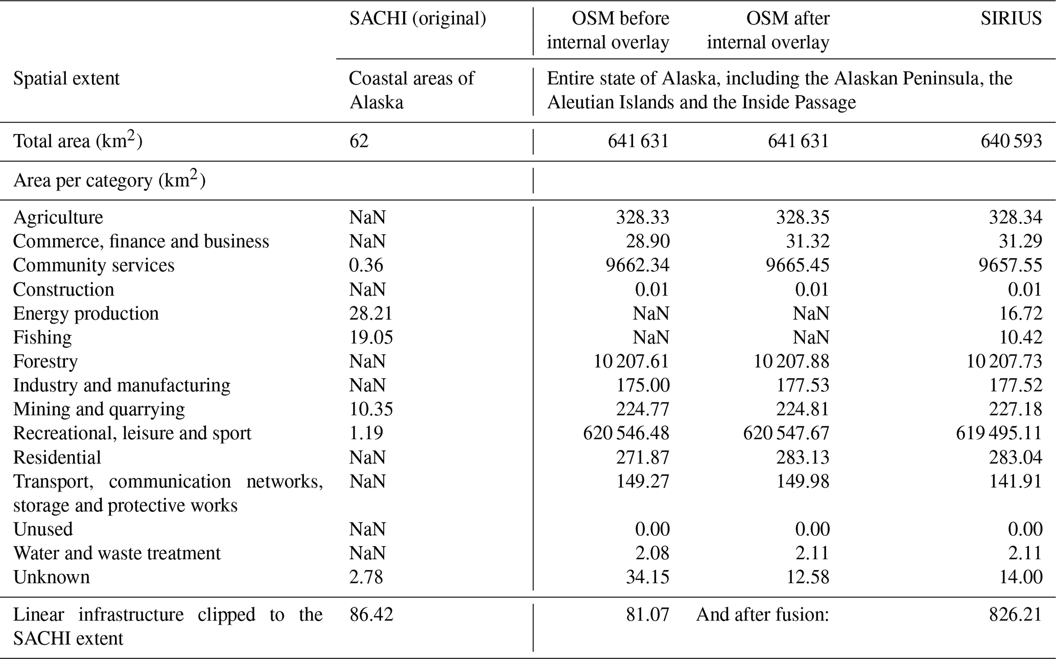
Table A4 Sample of the final Contaminated Sites dataset. The columns “Hazard ID”, “Borough” and “Status” (“IC” stands for “institutional controls”) were given in the original file, whereas the first and last dates, cleanup days, contaminated medium and contaminant information were derived using simple text-mining tasks (refer to Sect. 2.2.3).

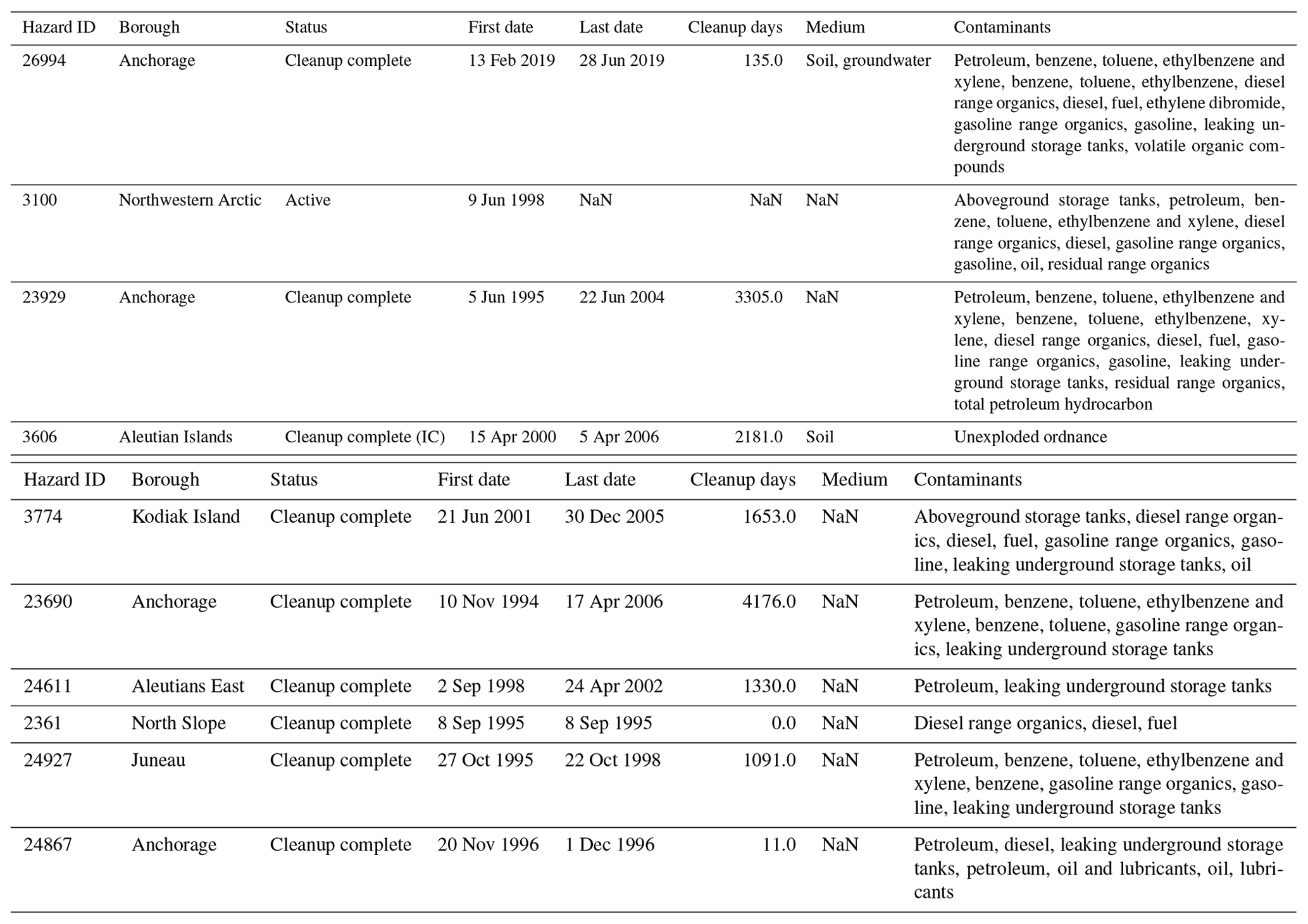
Table A5 Abbreviations indicating the toxic substances and contaminant-related containment structures. Source: Alaska DEC glossary (State of Alaska Department of Environmental Conservation, 2023b).

Appendix B: Application code snippets

import geopandas as gpd

## load GPKG file
geopackage_path = "/path/to/geopackage/PermaRisk_RRNetworkPolygonal_v01_r00.gpkg"

## load layers
polygon_layer = gpd.read_file(geopackage_path,
                              layer = 'SACHI_OSM_InfrastructureHIElements')
line_area_layer = gpd.read_file(geopackage_path,
                            layer = 'SACHI_OSM_InfrastructureHIElements_RRNetwork')
points_layer = gpd.read_file(geopackage_path,
                             layer = 'DEC_ContaminatedSitesAK')

## join IS-HI polygon and line layer
polygon_layer = polygon_layer.append(line_area_layer)

## create query
subset = gpd.sjoin(polygon_layer, points_layer, how='inner', predicate='intersects')
dfcount = subset.groupby('LUCAS')['geometry'].count().rename('pointcount').reset_index()