the Creative Commons Attribution 4.0 License.
the Creative Commons Attribution 4.0 License.
 | 02 Aug 2024
IAPv4 ocean temperature and ocean heat content gridded dataset
Yuying Pan
Zhetao Tan
Huayi Zheng
Yujing Zhu
Wangxu Wei
Huifeng Yuan
Guancheng Li
Hanlin Ye
Viktor Gouretski
Yuanlong Li
Kevin E. Trenberth
John Abraham
Yuchun Jin
Franco Reseghetti
Xiaopei Lin
Bin Zhang
Gengxin Chen
Michael E. Mann
Jiang Zhu
Ocean observational gridded products are vital for climate monitoring, ocean and climate research, model evaluation, and supporting climate mitigation and adaptation measures. This paper describes the 4th version of the Institute of Atmospheric Physics (IAPv4) ocean temperature and ocean heat content (OHC) objective analysis product. It accounts for recent developments in quality control (QC) procedures, climatology, bias correction, vertical and horizontal interpolation, and mapping and is available for the upper 6000 m (119 levels) since 1940 (more reliable after ∼ 1957) for monthly and 1°×1° temporal and spatial resolutions. IAPv4 is compared with the previous version, IAPv3, and with the other data products, sea surface temperatures (SSTs), and satellite observations. It has a slightly stronger long-term upper 2000 m OHC increase than IAPv3 for 1955–2023, mainly because of newly developed bias corrections. The IAPv4 0–2000 m OHC trend is also higher during 2005–2023 than IAPv3, mainly because of the QC process update. The uppermost level of IAPv4 is consistent with independent SST datasets. The month-to-month OHC variability for IAPv4 is desirably less than IAPv3 and the other OHC products investigated in this study, the trend of ocean warming rate (i.e., warming acceleration) is more consistent with the net energy imbalance at the top of the atmosphere than IAPv3, and the sea level budget can be closed within uncertainty. The gridded product is freely accessible at https://doi.org/10.12157/IOCAS.20240117.002 for temperature data (Cheng et al., 2024a) and at https://doi.org/10.12157/IOCAS.20240117.001 for ocean heat content data (Cheng et al., 2024b).
- Article
(20891 KB) - Full-text XML
-
Supplement
(399 KB) - BibTeX
- EndNote


Observational gridded products are essential for understanding the ocean, the atmosphere, and climate change; they support policy decisions and socioeconomic developments (Abraham et al., 2022; Abraham and Cheng, 2022; Cheng et al., 2022a). For instance, many of the climate indicators used in the Working Group I report of the 6th Intergovernmental Panel on Climate Change (IPCC-AR6-WG1) are based on gridded products (Gulev et al., 2021; IPCC, 2021), mainly because the raw oceanic data suffer from inhomogeneous data quality and irregular and incomplete data coverage (Abraham et al., 2013; Boyer et al., 2016; Cheng et al., 2022a; Meyssignac et al., 2019).
As more than 90 % of Earth's energy imbalance (EEI) in the past half-century has accumulated in the ocean, increasing ocean temperature (T) and ocean heat content (OHC) are essential climate variables for monitoring, understanding, and projecting climate change (e.g., Rhein et al., 2013; Hansen et al., 2011; Trenberth, 2022; Trenberth et al., 2009; von Schuckmann et al., 2020; Cheng et al., 2022a). OHC also impacts air–sea and ice–sea interactions and thus exerts a considerable influence on the other components of the climate system. It provides critical feedback through the energy, water, and carbon cycles (Cheng et al., 2022a; Trenberth, 2022; von Schuckmann et al., 2016). Substantial changes in ocean temperatures also profoundly impact ocean biogeochemical processes and ecosystems and are critical for ocean health and human society (Bindoff et al., 2019; Cheng et al., 2022a).
Many gridded T/OHC datasets have been produced by independent groups, and most of them are updated annually or more frequently (Cheng et al., 2022a; Good et al., 2013; Hosoda et al., 2008; Ishii et al., 2017; Levitus et al., 2012; Li et al., 2017; Meyssignac et al., 2019; Roemmich and Gilson, 2009). The most widely used products are at 1°×1° horizontal resolution and monthly temporal resolution from near-surface to about 2000 m depths. Some products utilize all available in situ observations and span at least half a century, prominent examples being the data products compiled by the Institute of Atmospheric Physics (IAP) (Cheng and Zhu, 2016; Cheng et al., 2017) from 1940 to the present, the Japan Meteorological Agency (JMA) (Ishii et al., 2017) from 1955 to the present, the National Centers for Environmental Information (NCEI), the National Oceanic and Atmospheric Administration (NOAA) from 1950 to the present (Levitus et al., 2012), and the University of California since 1949 (Bagnell and DeVries, 2021). As Argo data have achieved near-global upper 2000 m open-ocean coverage since ∼ 2005, many Argo-based or Argo-only gridded products are available. Examples include gridded products from SCRIPPS after 2004 (Roemmich and Gilson, 2009), the China Argo Real-time Data Center since 2005 (Li et al., 2017), and Copernicus since 2005 (von Schuckmann and Le Traon, 2011). These products usually span from ∼ 2005 to the present for the upper ∼ 2000 m. The data benefit from the high quality of Argo data but do not fully resolve the polar regions, shallow waters, and regions with complex topography.
In 2016, the IAP group provided its first gridded product for the upper 700 m of the ocean (Cheng and Zhu, 2016) by merging all available observations since 1960. With a revised mapping method and a thorough evaluation process with synthetic observations, an update (IAP version 3, IAPv3) became available in 2017 for the upper 2000 m of the ocean with data since the 1950s (Cheng et al., 2017). IAPv3 has supported scientific research, climate assessment reports, and monitoring practices (Bindoff et al., 2019; Gulev et al., 2021; WMO, 2022).
After the release of IAPv3, there was progress in observation data quality control and new or updated techniques for temperature data processing and reconstruction. For example, Gouretski et al. (2022) found that old Nansen cast bottle data contained systematic biases that impacted the T/OHC data before 1990. Revisions of the bias corrections are also available for Mechanical BathyThermograph (MBT) and eXpendable BathyThermograph (XBT) data (Cheng et al., 2014; Gouretski and Cheng, 2020). Tan et al. (2023) developed a new quality control system that advances the detection of outliers after accounting for the non-Gaussian distribution of local temperatures in determining the local climatological range. The impact of the inhomogeneous vertical resolution of temperature profiles was recognized previously (Cheng and Zhu, 2014) and received more attention recently (Li et al., 2020) with a new vertical interpolation approach (Barker and McDougall, 2020). Upgrading the product with new developments is important for better supporting ocean or climate research and climate assessments.
This paper discusses the revisions to the IAP ocean objective analysis product (IAPv4) since the publication of IAPv3 (Cheng et al., 2017). The data and methods are introduced in Sect. 2 and the results are presented in Sect. 3, with analyses of the character of IAPv4 on regional and global scales and on various timescales. The EEI and sea level budgets based on the new data product are also investigated. A summary and discussion are provided in Sect. 4, with some remaining issues and outlooks being discussed.
2.1 Data source
The majority of the in situ measurements used to create the data product come from the World Ocean Database (WOD), downloaded in December 2023. Data from all instrument types are used, including XBTs (Goni et al., 2019), Argo (Argo, 2000), conductivity–temperature–depth (CTD) profilers, MBTs, bottles, moorings, gliders, animal-borne ocean sensors (McMahon et al., 2021), and others (Boyer et al., 2018) (Fig. 1). There is a total of 17 634 865 temperature profiles from January 1940 to September 2023 (Zhang et al., 2024a, Fig. 1a). MBT, XBT, Nansen bottle, and CTD are the major instruments before ∼ 2005 (Fig. 1a, b). The spatial coverage of these data increased to > 30 % in 1960 and > 70 % in the late 1960s for -year resolution. After ∼ 2005, there is a huge number of glider (GLD) and animal-mounted pinniped-borne (APB) data, and as they are mainly distributed in the polar regions (APB) and coastal regions (GLD) (Fig. 1a), their spatial coverage is usually less than 5 % for -year resolution. By contrast, the Argo data cover most of the global open ocean since ∼ 2005 (Fig. 1b).
Argo data are processed following the recommendations of the Argo community. Adjusted data are used where applicable. Both delayed- and real-time Argo data have been incorporated into IAPv4. As real-time Argo data have only passed automated, simple quality control (QC) tests in real time, these data may still contain temperature, pressure, and salinity values affected by unknown errors. However, through a sensitivity study, Cheng (2024) indicated that including real-time Argo data does not bias the OHC calculation for the IAP analysis. Nevertheless, IAP data are updated frequently (every 1–3 months): each time the updated Argo data are used, the T/OHC fields are recalculated following the recommendation by the Argo group (Wong et al., 2020). The data from the Argo floats in the “grey list” have been removed from the calculation (https://data-argo.ifremer.fr/, last access: 1 December 2023).
To complement the WOD with relatively fewer data in the Arctic and coastal regions of the northwestern Pacific, this presented product also uses data from other sources. The majority of these data are from the Chinese Academy of Sciences Ocean Science Data Center (Zhang et al., 2024a, b), and some data have been rescued from old documents of marine surveys. All these data are publicly available. There are a total of 85 990 additional temperature profiles, about 0.50 % of the data, which is expected to improve the reconstruction in these data-sparse regions (compared with IAPv3 and the other products).
The in situ data have been processed as described in a flowchart in Fig. 2. In the following sections, the key techniques of the data processing are introduced.
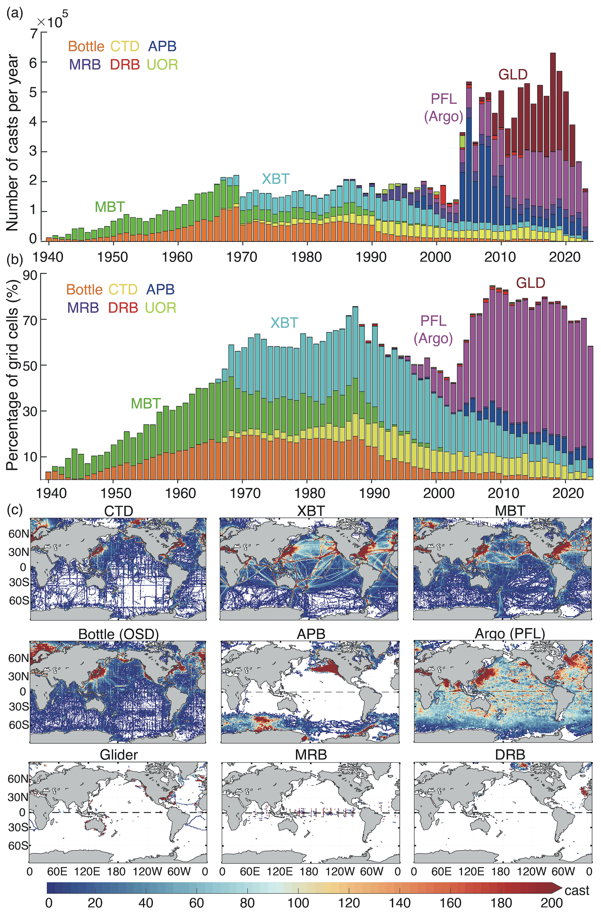
Figure 1(a) Yearly number of temperature casts for different instruments. (b) Percentage coverage (%) of ocean data for each instrument, calculated as the ratio between the number of -year grid cells observed by each instrument and the total number of ocean grids. (c) Number of subsurface temperature casts in 1° grid boxes from 1940 to 2023 collected by different instruments: CTD (conductivity–temperature–depth), XBT (eXpendable BathyThermograph), MBT (Mechanical BathyThermograph), bottle, APB (animal-mounted pinniped-borne), PFL (profiling floats, i.e., Argo), GLD (glider), MRB (moored buoy), and DRB (drifting buoy).
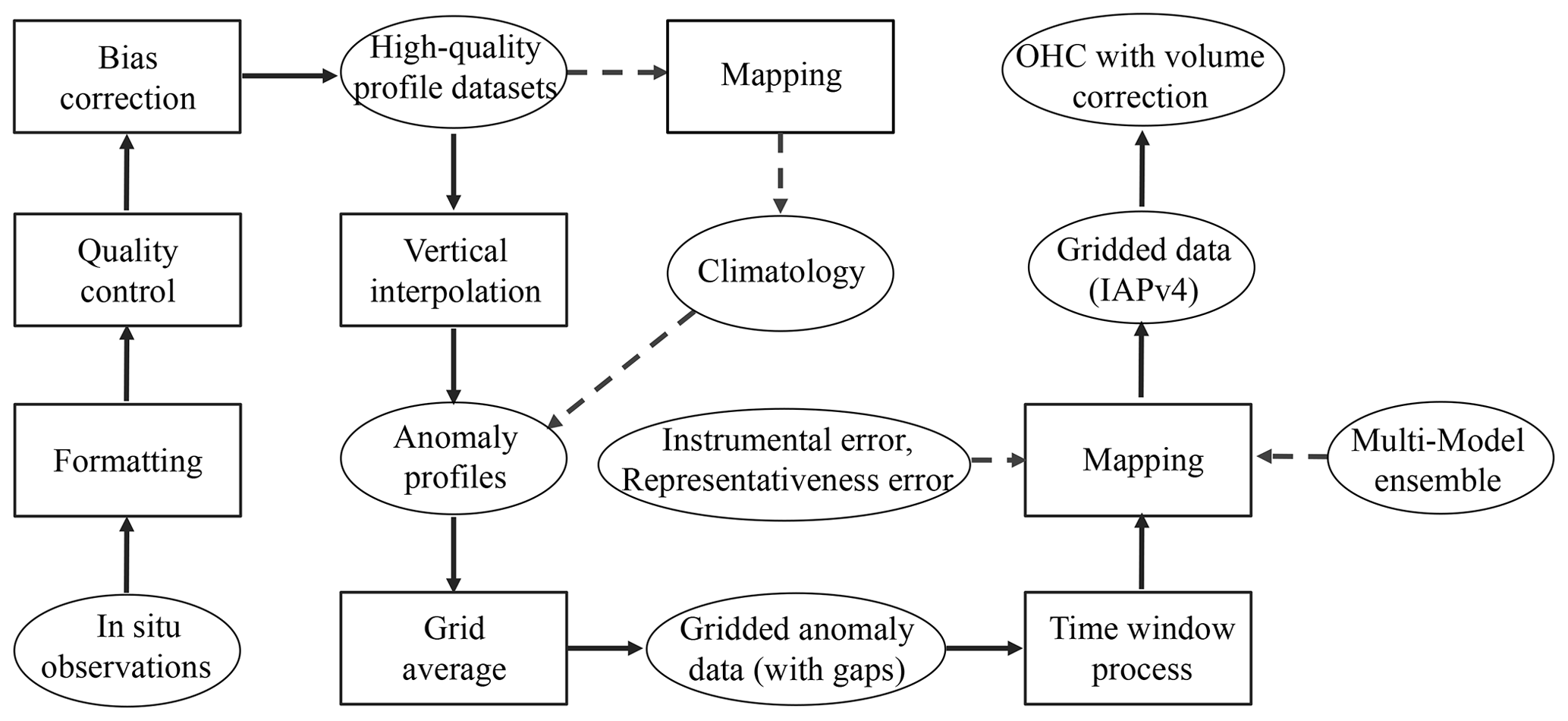
Figure 2Flowchart of the IAP data reconstruction processes from the raw in situ observations to gridded data (IAPv4) and OHC estimates. The ellipses indicate the data (including the data for error estimates), and the rectangle boxes show the techniques used to process the data.
2.2 Data quality control
The QC procedure aims to identify spurious measurements (including outliers) and data with incorrect metadata through a set of quality checks and ensures the quality of the in situ dataset (Tan et al., 2022). There is growing evidence that QC is critical for accurate temperature or OHC reconstruction, as shown by Tan et al. (2023), where two different QC systems produced a difference of approximately 15 % (∼ 7 %) in the 0–2000 m OHC trend from 1955–1990 (2005–2021). Unfortunately, the impact of QC on OHC estimates has not been evaluated in previous community assessments of T/OHC uncertainty (Boyer et al., 2016; Lyman et al., 2010). In this study, the QC procedure follows the CAS-Ocean Data Center (CODC) Quality Control system, named CODC-QC (Tan et al., 2023), where only the “good” data (flag = 0) are used (this means the observations passed all distinct checks).
The CODC-QC system (Tan et al., 2023) has the following strengths, which make it particularly suitable for T/OHC reconstruction.
-
A new local climatological range is defined in this CODC-QC system to identify outliers. Unlike many existing QC procedures, no assumption is made of a Gaussian distribution law in the new approach, as the oceanic variables (e.g., temperature and salinity) are typically skewed. Instead, the 0.5 % and 99.5 % quantiles are used as thresholds in CODC-QC to define the local climatological parameter ranges.
-
Local climatological ranges change with time to account for the long-term trends of ocean temperature accompanied by more frequent extreme events (e.g., Oliver et al., 2021; Sun et al., 2023). Previously, the use of the static local ranges tended to remove too many “extreme values” (at the tails of the temperature distributions) associated with climate change in recent years that were actually real, leading to a QC-procedure-related bias in the gridded dataset and OHC estimate (Tan et al., 2023).
-
In addition, local climatological ranges for the vertical temperature gradient are constructed to account for the variability of “vertical shape”, increasing the ability of the scheme to identify spurious profiles.
-
The QC procedure is instrument-specific, accounting for characteristics inherent to particular instrumentation types. For example, XBT digital recording systems are allowed to continue to record beyond the rated terminal depth suggested by manufacturers (T7/DB probes below 760 m; T4/T6 probes below 460 m; T5 probes below 1830 m). Below the rated maximum depth, the XBT wire often breaks, leading to a characteristic change in recorded temperature values. The new QC procedure effectively identifies such profiles.
-
The thorough evaluation of the QC procedure performance and the application of the QC procedure to the manually quality-controlled datasets (Thresher et al., 2008; Gouretski and Koltermann, 2004) demonstrated the effectiveness of the proposed scheme in removing spurious data and minimizing the percentage of mistakenly flagged good data.
Being applied to the entire temperature profile dataset, the CODC-QC procedure identifies 6.22 % of all the temperature measurements as outliers. The rejection rates (the definition follows Tan et al., 2023) vary among the instrumentation types (3.73 % for CTD, 1.97 % for Argo, 12.06 % for XBT, 4.93 % for MBT, 6.54 % for bottle, 5.92 % for APB, 4.54 % for DRB, and 2.55 % for MRB). The overall percentage of outliers decreases over time from ∼ 5 % in the 1940s to ∼ 2.5 % in the 2020s, reflecting the progressive improvement of the instrumentation (Fig. 3). A rejection rate maximum (∼ 12 %) during 2000∼ 2010 is linked to the XBT data, which are especially abundant in the 800–1100 m layer and are characterized by a higher rejection rate below the maximum depth (Tan et al., 2023). The generally higher rejection rate below 4000 m is related to the gross errors (e.g., measurements cooler than −2 °C, big spikes) and the occurrence of the constant values (the recorded values do not change with depth). For example, the higher rejection rate from 2008 to 2009 below 4000 m is because of the gross errors in the CTD data.
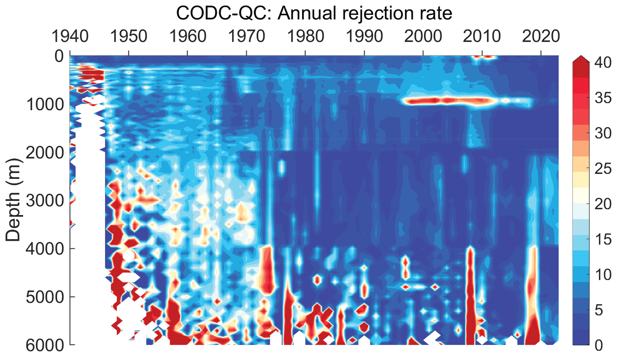
Figure 3The rejection rate (%) of temperature observations after CODC-QC as a function of calendar year and depth.
2.3 Bias correction
It is well known that data from several instrument types can exhibit biases in both temperature and depth. Temperature profiles obtained using XBTs and MBTs provide an example of biased data, especially because of uncertainties in the depth of measurement. Gouretski and Koltermann (2007) demonstrated their significant impact on the magnitude and variability of the global OHC estimates. That study triggered a series of publications where different bias correction schemes were suggested for XBT (Gouretski and Reseghetti, 2010; Abraham et al., 2013; Cheng et al., 2016; Levitus et al., 2009; Wijffels et al., 2008), MBT (Gouretski and Cheng, 2020; Levitus et al., 2009), APB (Gouretski et al., 2024), and other instruments (Fig. 2). In the compilation of IAPv4, newly developed bias correction schemes are applied.
The XBT temperature bias was found to be generally positive, as large as ∼ 0.1 °C before 1980 on the global 0–700 m average, diminishing to less than 0.05 °C after 1990 (Gouretski and Koltermann, 2007; Wijffels et al., 2008). Here, we use an updated XBT bias correction scheme (Cheng et al., 2014, CH14) to correct both depth and temperature biases in XBT data, following the community's recommendation (Cheng et al., 2016; Goni et al., 2019). The depth and temperature biases depend on ocean temperature, probe type, manufacturer, and time. An intercomparison among several correction schemes rated the CH14 scheme the most successful (Cheng et al., 2018). Using XBT and collocated CTD data, we updated the CH14 scheme by recalculating bias corrections between 1966 and 2016 and extending them for the years 2017–2023.
Comparison with collocated reference CTD profiles recently revealed significant biases in the old hydrographic profiles obtained by means of Nansen bottle casts (Gouretski et al., 2022). Both depth and temperature measurements of bottle casts were found to be biased, and the proposed correction scheme was also implemented in IAPv4. The thermal bias is related to the time needed to bring the mercury thermometers into equilibrium with the ambient temperature after the completion of the hydrographic cast. The depth bias indicates an overestimation of the bottle depth due to the wire's deviation from the vertical position and is mostly related to the hydrographic casts where the thermometrical method of sample depth determination was not used. The correction scheme includes a constant thermal bias of −0.02 °C and a depth- and time-varying depth bias.
The MBT bias is as large as 0.28 °C before 1980 for the global average and reduces to less than 0.18 °C after 1980 for the 0∼ 200 m average. IAPv3 used the Ishii and Kimoto (2009) (IK09) scheme to correct MBT bias, while a new scheme proposed by Gouretski and Cheng (2020) (GC20) is adopted in IAPv4. This shift is made because our assessment indicates undercorrection of MBT bias by the IK09 scheme within the upper 120 m and overcorrection in the deeper layer, whereas GC20 corrects both depth and temperature biases. GC20 also found MBT bias to be country-dependent, which is explained in terms of different instrumentation characteristics and working procedures. Therefore, the time-varying bias corrections are applied separately for the MBT profiles obtained by ships from the United States, the Soviet Union/Russia, Japan, Canada, and the United Kingdom. Data from all other countries are corrected using a globally averaged correction.
Finally, thermal biases were recently reported for the data obtained by different kinds of data loggers attached to marine mammals (APB). Gouretski et al. (2024) analyzed temperature profiles obtained between 2004 and 2019 at the high and moderate latitudes of both hemispheres. Comparison with the collocated reference CTD and Argo float data revealed a systematic negative thermal offset (average value −0.027 °C) for mammal temperature profiles from SRDLs (satellite-related data loggers). For the less accurate data from TDRs (temperature–depth recorders), the comparison revealed a small positive temperature bias of 0.02 °C and a depth (pressure) bias indicating depth overestimation.
2.4 Climatology
For IAP and other data product generators, horizontal interpolation (mapping) is applied to a temperature anomaly field after removing a monthly climatology; thus, a predefined climatology field with an annual cycle is mandatory (Fig. 2). The accuracy of the climatology field is one of the key sources of uncertainty in reconstruction because an error in climatology will propagate to the anomaly field and impact the spatial dynamical consistency and accuracy of the reconstruction (Cheng and Zhu, 2015; Lyman and Johnson, 2014; Boyer et al., 2016).
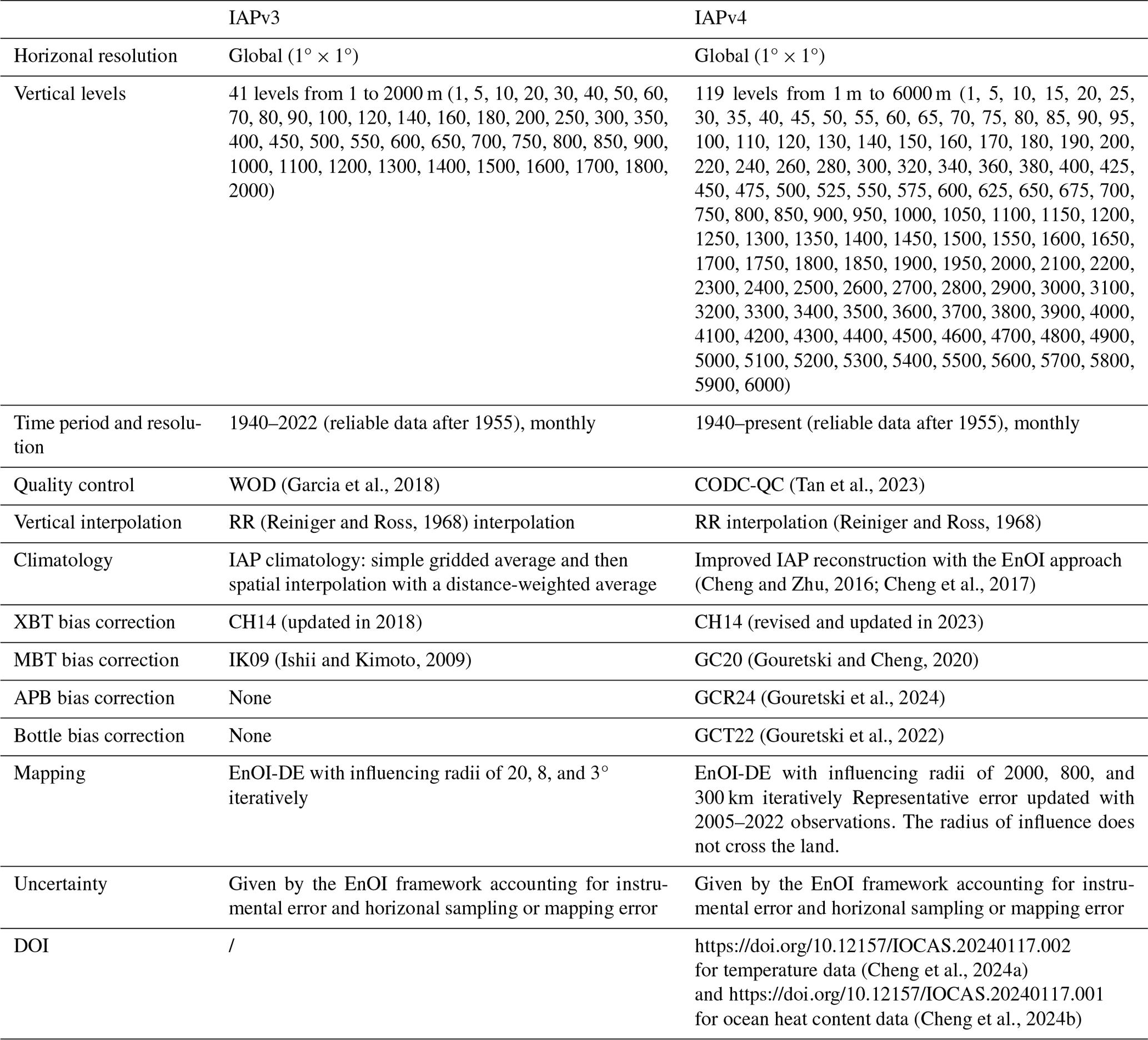
In IAPv4, the adjusted mapping procedure (see below) has been applied to reconstruct the climatology field (Table 1). The merit of using IAP mapping for climatology is its ability to better represent the spatial anisotropy of temperature variability (non-Gaussian distribution). Unlike IAPv3, where the 1990–2005 reference period was used, IAPv4 uses data between 2006 and 2020 to construct 12 monthly climatologies, taking advantage of more reliable data combined with better and more homogeneous spatial and temporal coverage in the last 2 decades (Table 1). Following the recommendation in Cheng and Zhu (2015), a relatively short period of 15 years is used because a climatology constructed with a longer period of data will result in different baselines at different locations (i.e., the baseline shifted to earlier years at the middle latitudes of the Northern Hemisphere and shifted to more recent years in the Southern Hemisphere), and this inconsistency will violate the spatial structure of the anomaly field (Cheng and Zhu, 2015). Recent developments from other groups, such as Li et al. (2022), include the choice of a short-period climatology.
IAPv4 used an 800 km influencing radius in its climatology reconstruction, smaller than the 20° for IAPv3, to more properly account for the rapid change in temperatures with distance. There is necessarily a tradeoff between data availability and the size of the influencing radius. Using radii smaller than 500 km does not ensure global fractional coverage (defined as the fraction of the total ocean area obtained by the mapping method) because of data sparseness (Cheng, 2024). As our tests suggest, using 500∼ 800 km results in very similar reconstructions of climatology. Therefore, 800 km is adopted to have more robust and stable data sampling.
2.5 Vertical interpolation
The vertical resolution of ocean temperature profiles changed dramatically over time, which was associated with instrument evolution and the increase in data storage capability. For instance, the global mean vertical resolution at the 500 m level changed from ∼ 100 m in the 1960s to less than 10 m during the 2010s (Li et al., 2020). Vertical interpolation of the raw profiles at standard levels is a critical process (Fig. 2): Cheng and Zhu (2014) indicated that the use of linear or spline vertical interpolation methods can bias the temperature reconstruction and OHC estimation (Barker and McDougall, 2020; Li et al., 2020; Li et al., 2022). IAPv3 used the Reiniger and Ross (1968) (RR) method. Recently, Barker and McDougall (2020) proposed a new approach using multiple piecewise cubic Hermite interpolating polynomials (PCHIPs) to minimize the formation of unrealistic water masses by the interpolation procedure.
Because the largest difference between the interpolation methods is found mostly for the low-resolution profiles (e.g., old Nansen casts), in practice, extremely low-vertical-resolution profiles had to be removed to reduce the uncertainty in interpolation. In IAPv4, this procedure is optimized compared to IAPv3, and only parts of profiles with a sufficient vertical resolution are used. The thresholds for the vertical resolution are set to 50 m in the upper 200 m, 200 m between 200 and 1000 m, 500 m between 1000 and 2000 m, and 600 m between 2000 and 6000 m. As no interpolation method can adequately interpolate temperature for the vertical resolution beyond these thresholds, interpolation is not performed in such cases to avoid errors (these extremely low-resolution data are not used in further processing). Under this limitation for IAPv4, we still apply the RR method for temperature profiles.
Finally, IAPv4 extends the set of standard vertical levels with a total of 119 levels from 1 to 6500 m (79 levels within the upper 2000 m) compared to 41 levels in IAPv3 between 1 and 2000 m (Table 1). The increase in vertical resolution is critical for accurately representing the mixed layer and other high-gradient regions, as investigated below.
2.6 Grid average and mapping
The anomaly profiles are obtained by subtracting the monthly mean climatology from the vertically interpolated profiles. These anomalies are then averaged (arithmetic mean) into a 1° × 1° grid at each standard level (1° × 1° gridded average field) (Fig. 2). Due to the general data sparsity, variable time windows (longer than 1 month) are used for monthly reconstructions to ensure a truly global analysis (Supplement Table S1). This process takes advantage of the larger persistence of anomalies (generally smaller monthly and interannual variability) in the deep ocean than in the upper ocean, and thus it is physically grounded. Specifically, after 2005, data within a 3-month window are merged to provide a monthly reconstruction for each layer of the upper 1950 m. Before 2005, a time-varying and depth-varying time window is used, and it is generally smaller in the upper ocean and wider in the deeper ocean (Table S1). Below 2000 m, a 5-year (60-month) window is adopted. The use of a time window will reduce the monthly variance compared to the other datasets, which is likely too high compared with independent Earth energy imbalance data at the top of the atmosphere (Trenberth et al., 2016).
Mapping interpolates the gridded (e.g., box-averaged) observations horizontally into a spatially complete map (Fig. 2) because not all 1° × 1° boxes are filled with data (Fig. 2). IAPv4 adopted a similar mapping approach (ensemble optimal interpolation with a dynamic ensemble: EnOI-DE) to IAPv3 introduced in Cheng and Zhu (2016) and Cheng et al. (2017) but with the following modifications.
-
The largest influencing radius was changed from 20° in the upper 700 m (25° at 700–2000 m) in IAPv3 to 2000 km in the upper 700 m (2500 km at 700–6000 m) in IAPv4, to account for the reduced distance between two longitudes from the tropical to polar regions. This change mainly helps to improve the reconstruction in the high-latitude regions.
-
The three iterative runs are taken to effectively bring in different scales of variability with influencing radii changing from 2000 km (2500 km at 700–6000 m) to 800 and 300 km, respectively, based on the tests presented in Cheng and Zhu (2016) and Cheng et al. (2017).
-
For each month, IAPv3 used 40 model simulations (historical runs) from the Coupled Model Intercomparison Project Phase 5 (CMIP5) to provide a flow-dependent ensemble, which is then constrained by observations to provide optimized spatial covariance. IAP mapping uses model-based covariance because we argue that spatial covariance can never be satisfactorily parameterized by some simple basic functions (such as Gaussian ones) given its complexity. With model-based, flow-dependent, and dynamically consistent covariance, IAP mapping provides a more realistic reconstruction than other approaches based on Gaussian parameterized covariance, as evaluated by many studies (Cheng et al., 2017, 2020; Dangendorf et al., 2021; Nerem et al., 2018).
-
The observation error variance (R), which represents the error of the observations, is updated in IAPv4 as follows. R consists of both the instrumental error (Re) due to inaccuracy and the representativeness error (Rr) due to the need to represent the spatial (at 1° × 1° and 1 m standard grid depths) and temporal (1-month) averages from a limited number of observations (Cheng and Zhu, 2016):
where M observations exist for a given grid cell. Ei is the instrument's precision for each individual observation, assuming a random error (the basic assumption is that, after bias correction, the systematic errors can be eliminated). The Re in each grid cell is set to the mean of the typical precision of the different instruments contributing data in the cell, which is set according to the IQuOD (International Quality-Controlled Ocean Database) specification (Cowley et al., 2021). σ2 represents the variance of the various temperature measurements against the monthly mean value. The data from 2005 to 2022 are used to calculate σ2 in each grid because of greater data abundance and quality compared to earlier times.
As the representativeness error (Rr) is expected to be flow-dependent (i.e., the error is expected to be higher in the regions of higher variability), more observations are required to represent the mean value. Figure 4 shows a larger variance (σ2) in the boundary current regions and near the Antarctic Circumpolar Current (ACC) in the upper ocean (e.g., 10, 200, and 500 m). At 200 m, it shows a larger σ2 in the western Pacific Ocean, corresponding to the large thermocline variations at this layer. Below 1000 m, larger σ2 values occur along the ACC frontal regions and in the North Atlantic Ocean because of stronger mixing and convection in these regions.
The uncertainty in the derived gridded reconstruction is also based on the EnOI framework formulated by Cheng and Zhu (2016). The uncertainty accounts for instrumental, sampling, and mapping errors. Other error sources, including the choice of climatology, vertical interpolation, bias corrections, and QC, are not considered in this uncertainty estimate. Therefore, a more thorough uncertainty quantification method is needed, and this is under development in a separate study.
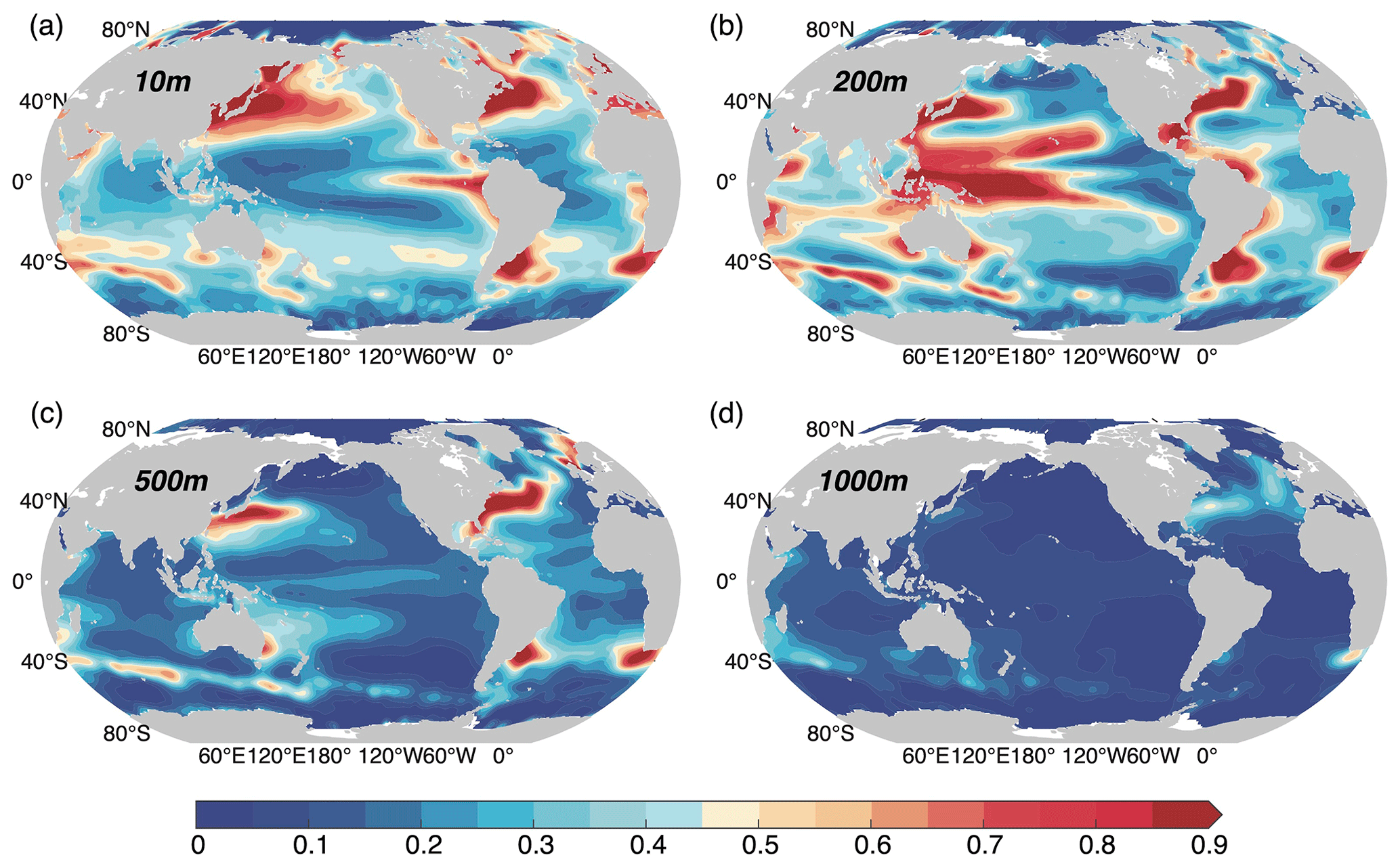
Figure 4Variance (σ2; °C2) of ocean temperature at several representative depths: (a) 10, (b) 200, (c) 500, and (d) 1000 m.
2.7 OHC calculation and volume correction
Based on the gridded temperature reconstruction (Table 1), the OHC in each grid is calculated as OHC following the Thermodynamic Equation Of Seawater – 2010 (TEOS-10) standard, where cp is a constant of ∼ 3991.9 J (kg K)−1 according to the new TEOS-10 standard formulation as a conservative temperature and absolute salinity are used, ρ is the potential density (kg m−3), and T is the conservative temperature calculated from in situ temperature (°C; here it is the anomaly relative to the 2006–2020 baseline) (Cheng et al., 2022a).
As OHC is an integrated metric over a specific ocean volume, properly identifying ocean volume is critical, especially in shallow waters. Previous studies found a 10 %–20 % difference in the OHC trend in recent decades between different land–ocean masks (von Schuckmann and Le Traon, 2011; Meyssignac et al., 2019; Savita et al., 2022). Specifically, in marginal sea areas with complex topography, 1° × 1°×Δz grid boxes (where Δz is the depth range of the grid box) near coasts and islands typically cover both ocean and land areas but are assigned to represent land or ocean only. Thus, the gridded ocean temperature datasets are subjected to errors from inaccurate land–sea attribution. Here, we offer a volume correction (VC) for these grid boxes to improve the OHC estimate as follows.
For each 1° × 1° × Δz grid box, we introduce a VC factor (denoted as FVC) to correct the OHC values: OHC × . First, we assume the seawater volume distribution in 1 arcmin topographic data of ETOPO1 to be the “truth”. No correction is needed if a box is assigned to ocean according to ETOPO1 data; thus, FVC=1. If a fraction of a 1° × 1° × Δz grid box is land according to ETOPO1 and if IAP data include T/OHC values, the FVC is represented by the fraction of the ocean volume in this box (illustrated in Fig. 5), and the volume for OHC calculations can be corrected with FVC(i). In a grid box, if there are no IAP data (i.e., they are land according to the IAP mask) but this box contains some ocean volume according to ETOPO1 data, we define FVC(a) again as the fraction of the ocean volume in this box, and then this FVC(a) is added to the adjacent grid boxes where there are values in the IAP data. If all the adjacent grid boxes contain no data, the volume is equally redistributed to the diagonal boxes (Fig. 5). The volume is discarded if there are no data in all the adjacent and diagonal boxes.
With this approach, the VC factor in each grid box is a sum of two components, a local adjustment FVC(i) and a redistribution FVC(a) from the adjacent grids:
To avoid misidentification of sea ice, we performed VC only on the global grid points within 60° S–60° N. Eventually, we obtained a three-dimensional FVC that fits the IAP grids (119 × 360 × 180; depth coverage to 6000 m) and used it to compute OHC. The VC was applied to ∼ 15 % of all the 1° × 1° × Δz grid boxes of the IAPv4 ocean grid boxes (with FVC≠1) for all the 0–6000 m ocean and ∼ 10 % grid boxes of the upper 2000 m. Since the open ocean accounts for the vast majority of the global ocean volume, the influence of the VC method on the global OHC trend is small. For example, the upper 2000 m OHC trend with VC is ∼ 0.15 % (∼ 0.45 %) smaller than without VC from 1958–2023 (2005–2023) for IAPv4. However, it can significantly affect regional OHC estimates, especially in regions with complex topography. For example, the Maritime Continent region's 0–2000 m OHC trend is reduced by 6.9 % (4.2 %) after applying VC from 1958–2023 (2005–2023) (Jin et al., 2024).
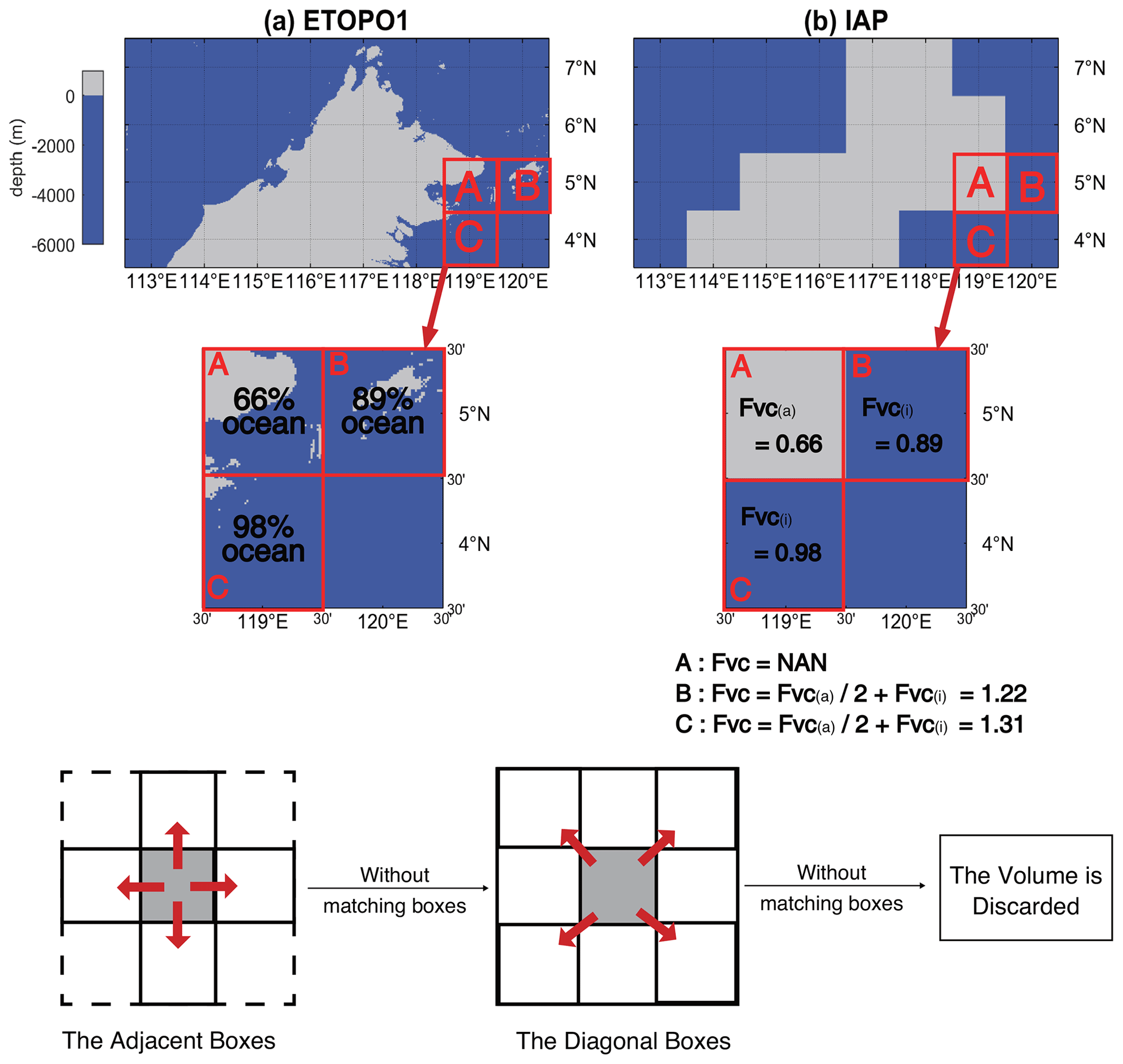
Figure 5An example explaining the volume correction algorithm. (a) Bathymetry derived from ETOPO1. (b) Bathymetry in IAPv4 analysis.
2.8 Independent datasets for comparison and evaluation
Four sea surface temperature (SST) datasets are used to evaluate the uppermost layer (1 m) of IAPv4, i.e., the Extended Reconstructed SST version 5 (ERSST5) (Huang et al., 2017), the Japan Meteorological Agency Centennial Observation-Based Estimates of SSTs version 1 (COBE1) (Ishii et al., 2005) and its version 2 (COBE2) (Hirahara et al., 2014), and the Hadley Centre Sea Ice and Sea Surface Temperature dataset (HadISST) (Rayner et al., 2003). The anomalies relative to a 2006–2020 average were computed by removing the monthly climatology. Measurements of SST are made in situ by means of thermometers or are retrieved remotely from infrared and passive microwave radiometers on satellites (Kennedy, 2014; O'Carroll et al., 2019). Satellite SST observations began in the early 1980s. In situ SST observations go back to the 19th century and involve many different measurement methods, including wooden and later insulated metal buckets to collect water samples, engine room inlet measurements, and sensors on moored and drifting buoys (Kennedy, 2014). The subsurface temperatures are collected as “profiles” which contain multiple measurements at discrete vertical levels. Because of the differences in the observation systems, SSTs are fundamentally different in their temporal and spatial coverage and their temporal extent compared to the subsurface observations on which OHC estimates rely. SST measurements also have different uncertainty sources and error structures; thus, the two systems are typically treated as independent data sources and have been used for cross-validation (Gouretski et al., 2012).
An independent in situ observation dataset in the Labrador Sea is used to evaluate IAPv4. This dataset, provided by the Bedford Institute of Oceanography (BIO) (Yashayaev, 2007; Yashayaev and Loder, 2017), includes independently validated and bias-corrected data from multi-section hydrological surveys (i.e., AR7W) in the Labrador Sea, spanning from 1896 to 2020 (this study used 1960–2020 data). These data have not been incorporated into the WOD.
The capability of the new product to close the sea level budget and Earth's energy budget also provides tools for validation. A superior dataset should be capable of closing the sea level and Earth energy budgets. The total sea level change has been monitored using satellite altimetry since 1993 (from the University of Colorado at https://sealevel.colorado.edu/, last access: 10 May 2024). The ocean mass change has been derived from Jet Propulsion Laboratory (JPL) RL06.1Mv3 Mascon Solution Gravity Recovery and Climate Experiment (GRACE) and Gravity Recovery and Climate Experiment Follow-On (GRACE-FO) data since 2002 (Watkins et al., 2015). For long-term total sea level change since the 1950s, we use a tide-gauge-based reconstruction (Frederikse et al., 2020). During the same period, the estimates of the Greenland ice sheet, Antarctic ice sheet, land water storage, and glacier ice melt contributions from Frederikse et al. (2020) are used to derive the ocean mass change. To derive the steric sea level, IAP salinity data are used (Cheng et al., 2020). The temperature and salinity data are converted to the steric sea level based on the TEOS-10 standard (McDougall and Barker, 2011).
For the energy budget, the ice, land, and atmosphere heat content changes are from von Schuckmann et al. (2023) from 1960 to the present. Because of the less reliable data before the 1990s for land, sea ice, and ice sheets, the other set of land–atmosphere–ice data from 2005 to 2019 is used as in Trenberth (2022) to investigate the recent changes. The net radiation change at the top of the atmosphere is based on Clouds and Earth's Radiant Energy Systems (CERES) Energy Balanced and Filled (EBAF) data from Loeb et al. (2021) and Loeb et al. (2018) and Deep-C data from the University of Reading (Liu and Allan, 2022; Liu et al., 2017).
Several gridded ocean T/OHC gridded products are used here for intercomparison, including IAPv3 (Cheng et al., 2017), the EN4 ocean objective analysis product from the UK Met Office Hadley Centre (Good et al., 2013), the ocean objective analysis product (Ishii et al., 2017) (termed “ISH” hereafter) from the JMA, an Argo-only gridded product from SCRIPPS (Roemmich and Gilson, 2009) (termed “RG” hereafter), and an OHC product based on random forest regressions (termed “RFROM” hereafter) using in situ training data from Argo and other sources on a 7 d × ° × ° grid with latitude, longitude, time, SSH, and SST as predictors (Lyman and Johnson, 2023). Several datasets available in IPCC-AR6 (Gulev et al., 2023) are used for comparison, including the PMEL product from Lyman and Johnson (2014), machine-learning-based reconstruction of OHC by Bagnell and DeVries (2021), the BOA product based on refined Barnes successive corrections by the China Argo Real-time Data Center (Li et al., 2017), the International Pacific Research Center (IPRC) (2005–2020), von Schuckmann and Le Traon 2011 (KvS11), a machine-learning based reconstruction of OHC: Ocean Projection and Extension neural Network (OPEN) (Su et al., 2020), and a Green-function-based OHC estimate derived from SST (Zanna et al., 2019).
2.9 Trend calculation and uncertainty estimates
The trends in this study have been estimated using the locally weighted scatterplot smoothing (LOWESS) approach (Cheng et al., 2022b); i.e., we apply LOWESS to the time series (25-year window, equal to an effective 15-year smoothing), and then the OHC difference between the first and last years is used to calculate the trend. This approach provides an effective method of quantifying the local trend by minimizing the impact of year-to-year variability and start and end points.
Throughout this paper, a 90 % confidence interval is shown. The uncertainty in the trend also follows the approach in Cheng et al. (2022a) based on a Monte Carlo simulation. First, a surrogate OHC series is formed by simulating a new residual series (after removing the LOWESS smoothed time series) based on the AR(1) process and adding it to the LOWESS line. Then a LOWESS trendline is estimated for each surrogate. This process is repeated 1000 times, and 1000 trendlines are available. The 90 % confidence interval for the trendline is calculated based on ± 1.65 times the standard deviation of all 1000 trendlines of the surrogates. Secondly, the uncertainty in the rate of the OHC is estimated using the 1000 LOWESS trendlines: (1) calculating the rate based on the difference between the first and last annual mean values of the LOWESS trendline in a specific period and (2) calculating ± 1.65 times the standard deviation of the 1000 rate values.
3.1 Climatological annual cycle
The annual cycle of the OHC above 2000 m of IAPv4 is compared with IAPv3, ISH, EN4, RG, and RFROM (Figs. 6 and 7) for 2006–2020. There is a consistent annual cycle among different datasets for the global and hemispheric oceans. Globally, the ocean releases heat from boreal spring to fall and accumulates heat from boreal fall to spring, which is dominated by the Southern Hemisphere due to its larger ocean surface area (Fig. 6). The two hemispheres show opposite annual variations in OHC, associated with the annual change in solar radiation and different distributions of land and sea. For the global OHC above 2000 m, IAPv4 shows a positive peak in April and a dip in August, with a magnitude of OHC variation of 60.4 ZJ for IAPv4 (66.9 ZJ for IAPv3), consistent with the other datasets: 53.2 ZJ for ISH, 58.1 ZJ for EN4, 69.2 ZJ for RG, and 56.6 ZJ for RFROM (where 1 ZJ = 1021 J).
There are some unphysical variations in the OHC annual variations for IAPv3 (purple lines). For example, the global OHC shows large spikes in January and December and a big shift from September to October. By contrast, the other three data products show much smoother changes (Fig. 6a). The IAPv3 Arctic OHC (north of 69.5° N) shows a different phase change compared with the other datasets together with a big shift from September to December, and the magnitude of variability is much larger in IAPv3 than the other datasets (Fig. 6d). The improvement in IAPv4 is mainly because of the methodology improvements: IAPv3 used 1990–2005 data to construct a climatology which suffered from errors related to sparse data coverage, use of “degree distance” instead of “kilometer distance”, and other error sources. Therefore, the IAPv4 analysis presents a physically tenable OHC seasonal variation.
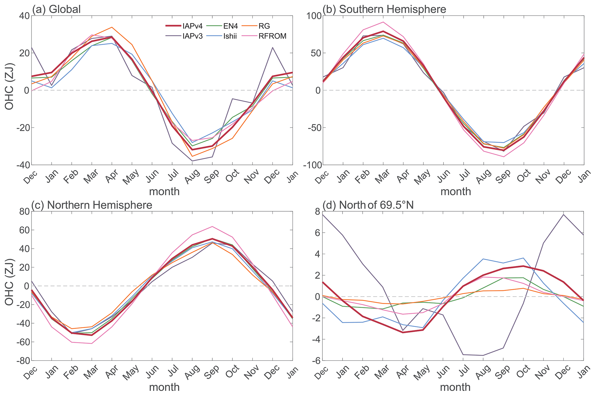
Figure 6Annual cycle of the OHC of the upper 2000 m for (a) the global oceans, (b) the Southern Hemisphere, (c) the Northern Hemisphere, and (d) the oceans north of 69.5° N. Five different data products are presented, i.e., IAPv4 (red), IAPv3 (black), ISH (purple), EN4 (green), RG (orange), and RFROM (pink).
IAPv4 OHC data show significant improvements in the Arctic region, reflected in both the spatial distribution and seasonal variation of OHC. In IAPv3, the maximum upper 2000 m OHC occurs in December, and the minimum OHC occurs in August. However, for IAPv4, the maximum amounts to 2.9 ZJ in October and decreases to a minimum of −3.4 ZJ in April. This estimate of the Arctic annual cycle is consistent with a constrained Arctic OHC estimate with atmospheric data by enforcing energy budget closure (Mayer et al., 2019). Furthermore, the spread of the OHC annual cycle in the Arctic region across different datasets is reduced from 5.2 to 2.5 ZJ, indicating a smaller uncertainty. The spatial OHC anomaly distribution in the Arctic region of IAPv4 is more spatially homogeneous than IAPv3, and IAPv3 appears as rays emerging from the pole which are not physical (Fig. 7). IAPv4 displays a consistent seasonal variation north of 69.5° N, mainly because of the changes in the influencing radius from “degrees” to “kilometers”.
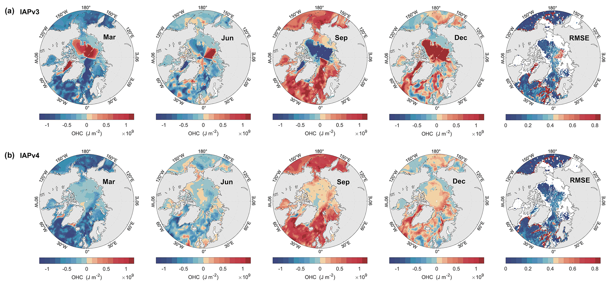
Figure 7Seasonal distribution of monthly mean upper 2000 m OHC anomalies and the root mean square error (RMSE) of 0–2000 m OHC between gridded data and in situ observations. For OHC anomalies, 4 months are shown: March, June, September, and December. The OHC anomalies are relative to the 2006–2020 annual mean. Panels (a) and (b) are for the IAPv3 and IAPv4 products, respectively. The panels in the last column are for the annual RMSEs for IAPv3 (upper) and IAPv4 (lower), respectively.
3.2 Mixed layer depth
Mixed layer depth (MLD) provides a crucial parameter of upper-ocean dynamics relevant for upper–deeper ocean and air–sea interactions. Spatial distributions of the MLD in March and August are shown in Fig. 8 for IAPv4, based on the criterion of ΔT=0.2 °C temperature for the 10 m depth temperature. As expected, the seasonal variations of the MLD are generally opposite in the Northern Hemisphere and Southern Hemisphere. The MLD shows a much stronger seasonal variation in the subtropics and at the midlatitudes (e.g., 20° ∼ 70° in both hemispheres) than in other regions (including the tropics, e.g., 20° S ∼ 20° N), which is manifested as a shallower MLD (∼ 20 m) in summer due to strong surface heating that increases stratification as well as a deeper MLD in winter (>70 m) because of surface cooling and increased surface wind creating stronger mixing.
In the Northern Hemisphere, the maximum MLD occurs during the wintertime in the subpolar North Atlantic deep-water formation regions (40° N ∼ 65° N), with values over 500 m in the Iceland Basin. In comparison, at the midlatitudes, the maximum of the MLD is generally less than 125 m in the wintertime. The MLD minimum in the Northern Hemisphere is in the summertime, and the values are mostly within 20 m. In the Southern Hemisphere, the MLD maximum values (deeper than 300 m) occur between 45 and 60° S (north of the Antarctic Circumpolar Current) in the boreal summer, when the year-round intense westerly winds occur. The minimum MLD in this region in the boreal winter is less than 70 m. The seasonal variation of the MLD has been well established by previous studies (Chu and Fan, 2023; de Boyer Montégut et al., 2004; Holte et al., 2017), and this evaluation confirms that IAPv4 temperature data are capable of reasonably representing the MLD. However, as pointed out by de Boyer Montégut (2004), the MLD estimated from the average temperature profiles might lead to an underestimation of the MLD by ∼ 25 % compared to the MLD computed from individual profiles based on the same 0.2 °C criterion method. This potential issue needs further investigation.
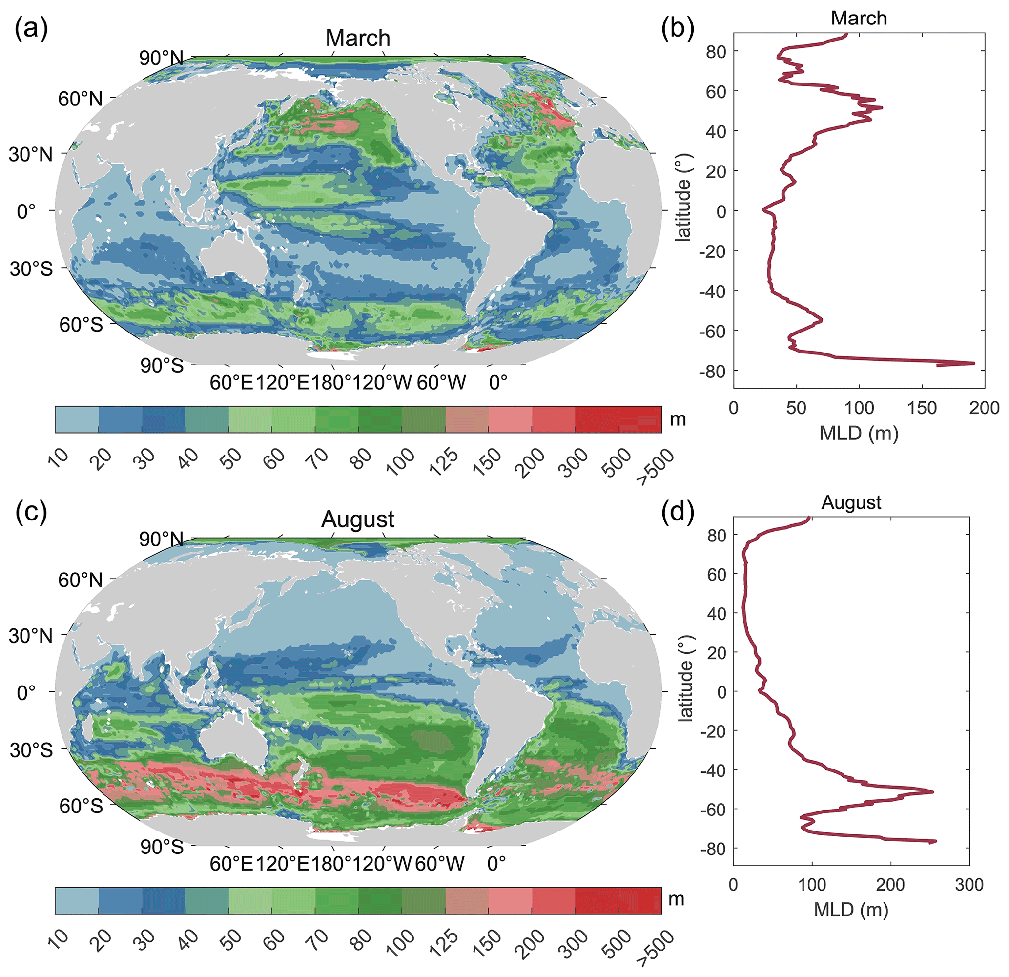
Figure 8Spatial pattern of the climatological mean MLD (a, c) and zonal mean MLD (b, d) in March (a, b) and August (c, d) estimated from IAPv4. Here, the MLD is calculated using the temperature difference criterion of ΔT=0.2° between the surface and 10 m depth.
3.3 Sea surface temperature
IAPv4 and IAPv3 temperature time series at 1 m depth (Fig. 9) are compared with four independent SST data products (ERSST5, HadISST, COBE1, and COBE2). All data products including IAPv4 show robust sea surface warming in the global ocean and the four main basins since 1955 (Fig. 9). Since the HadISST and COBE2 data did not include the year 2023, we compare the long-term SST trend from 1955 to 2022 using these products (Fig. 9f). The global mean IAPv4 SST rate between 1955 and 2022 is 1.01 ± 0.15 °C per century (90 % confidence interval – CI), which is within the range of the SST products (ranging from 0.78 to 1.05 °C per century). The 1955–2022 trend of IAPv4 SST is slightly weaker than IAPv3 for the global ocean (1.11 ± 0.16 °C per century) and all the ocean basins. The largest difference between IAPv4 and other SST products comes mainly from the Pacific Ocean and Southern Ocean before 1980 and is associated with sparser in situ observations for both SST and subsurface temperature data.
The spatial distribution of long-term SST trends over the 1955–2022 period provides insights into the data consistencies and differences. First, IAPv4 shows a pattern of SST trends consistent with the other datasets (Fig. 10). More rapid warming is found in the poleward western boundary current regions, such as the East Australian Current and the Gulf Stream. The stronger trends of ocean warming in the upwelling areas, such as the tropical eastern Pacific and the Gulf of Guinea, are identified by all the data products. The surface warming in the southern Indian Ocean for IAPv4 data is weaker than for IAPv3, ERSST5, and COBE2 but is more consistent with HadISST and COBE1. The surface cooling south of 60° S can also be found in all the datasets but with some discrepancies in magnitude and locations related to data sparsity. The tropical Pacific SST trends are mostly insignificant in the eastern and southeastern Pacific Ocean because of the strong interannual and decadal fluctuations (figure not shown).
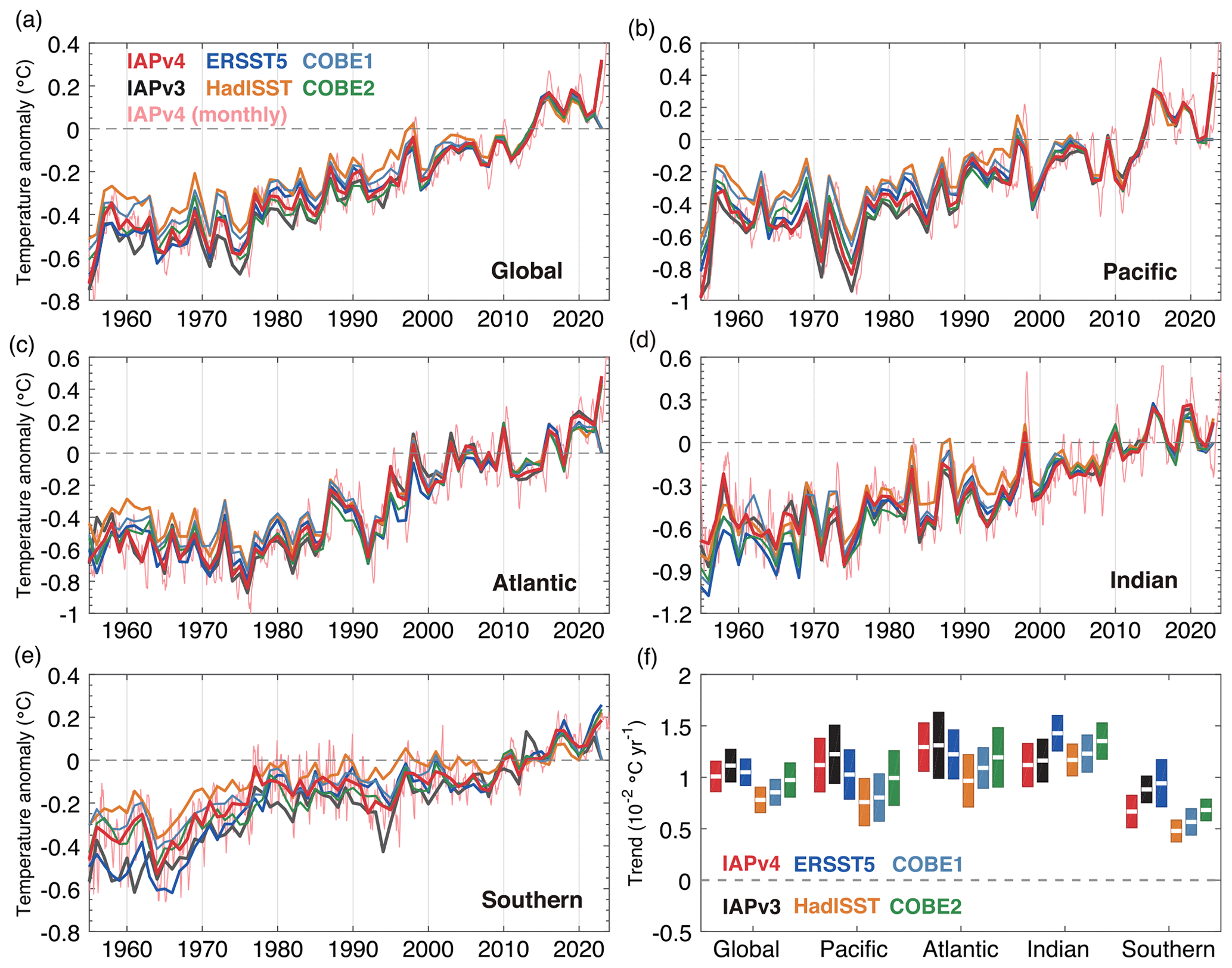
Figure 9Global and basin time series of SST change for IAPv4, compared with ERSST/HadISST/COBE1/COBE2 and IAPv3 from 1955 to the present. (a) Global, (b) Pacific, (c) Atlantic, (d) Indian, and (e) Southern oceans (south of 30° S) (°C). Panel (f) shows the warming rate from 1955 to 2022. The this pink line is the monthly time series of the IAPv4 SST, and the other time series are annual time series of the different datasets. The vertical scales are different for the different panels. All the anomaly time series are relative to a 2006–2020 baseline.
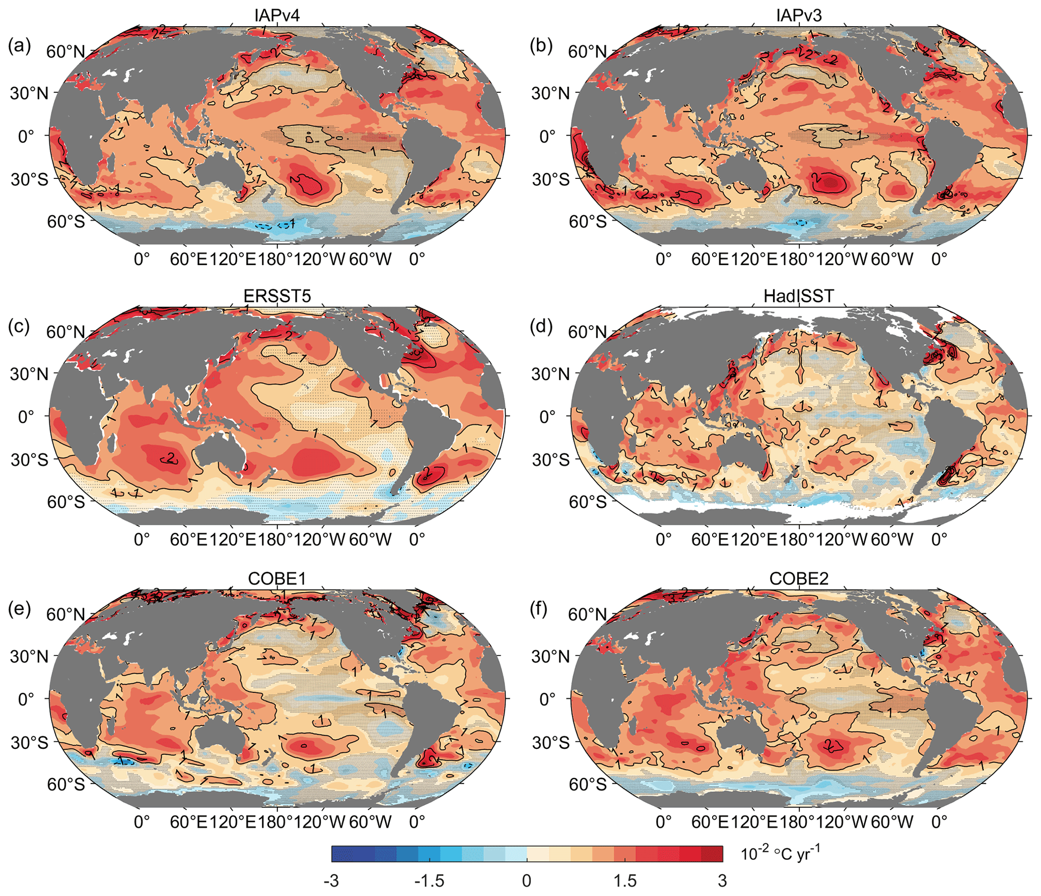
Figure 10Spatial maps of the SST long-term trends during the 1955–2022 period. (a) IAPv4, (b) IAPv3, (c) ERSST5, (d) HadISST, (e) COBE1, and (f) COBE2 (10−2 °C yr−1). The contour line interval is °C yr−1. The stippling indicates the regions with signals that are not statistically significant (90 % CI).
3.4 Global OHC time series
Global OHC time series for the 0–700, 700–2000, 0–2000, and 2000–6000 m layers of IAPv4 (Fig. 11) for 1955–2023 versus IAPv3 show robust ocean warming, with linear warming rates of 4.4 ± 0.2 ZJ yr−1 (0–700 m), 2.0 ± 0.1 ZJ yr−1 (700–2000 m), and 6.4 ± 0.3 ZJ yr−1 (0–2000 m). The long-term warming revealed by IAPv4 is greater than IAPv3 (4.1 ± 0.2 ZJ yr−1 for 0–700 m, 1.9 ± 0.1 ZJ yr−1 for 700–2000 m, and 6.0 ± 0.3 ZJ yr−1 for 0–2000 m). Before ∼ 1980, bottle bias correction reduces the time-varying systematic warm bias in Nansen bottle data and leads to a stronger warming rate from 1955 to 1990. The updated MBT and XBT corrections are mainly responsible for the difference between 1980 and 2000 (Cheng et al., 2014; Gouretski and Cheng, 2020). Data QC impacts the intraseasonal and interannual variation of the OHC time series (Tan et al., 2023). Also, because of the application of bottle, XBT, or MBT corrections, IAPv4 shows a stronger upper 2000 m ocean warming trend than most of the other available products assessed in Fig. 12.
From 2005 to 2023, the new IAPv4 product shows stronger warming than IAPv3. The mean upper 2000 m warming rates are 10.7 ± 1.0 ZJ yr−1 for IAPv4 and 9.6 ± 1.1 ZJ yr−1 for IAPv3 (Fig. 11), mainly because of the replacement of the WOD-QC system with the new CODC-QC system in IAPv4. Tan et al. (2023) indicated that the WOD-QC system had removed more extreme higher temperature values in the regions of warm eddies and marine heat waves than CODC-QC. The IAPv3 700–2000 m OHC shows a much bigger drop in 2018 than IAPv4 (Fig. 11b), while IAPv4 indicates an approximately linear 700–2000 m warming since 2005, resulting in stronger 700–2000 m warming in IAPv4 (3.6 ± 0.5 ZJ yr−1) than in IAPv3 (2.9 ± 0.5 ZJ yr−1). Compared with the other available products shown in Fig. 12, IAPv4 shows a similar 0–2000 m OHC trend to RFROM from 2005 to 2023 but with stronger warming trends than the two Argo-based products (BOA and SCRIPPS). From 1993 to 2023, IAPv4 showed a stronger 0–2000 m OHC trend than NCEI, Ishii, OPEN, and Zanna data and a slightly weaker trend than PMEL and RFROM (Fig. 12).
Since the 1990s, the World Ocean Circulation Experiment (WOCE) has provided a global network of abyssal ocean observations, sustained by repeated hydrological lines and the Deep Argo program (Katsumata et al., 2022; Roemmich et al., 2019; Sloyan et al., 2019). These high-quality data provide an opportunity to estimate deep OHC changes below 2000 m in this study. IAPv4 provides a new OHC estimate below 2000 m by collecting 5 years of data centered on each month. The result (Fig. 11d) indicates a robust abyssal (2000–6000 m) ocean warming trend since ∼ 1993 of 2.0 ± 0.3 ZJ yr−1. This is higher (within the uncertainty range) than the previous estimate of 1.17± 0.5 ZJ yr−1 in Purkey and Johnson (2010) but is consistent with the recent assessment showing the acceleration of deep-ocean warming in the southwestern Pacific Ocean (Johnson et al., 2019).
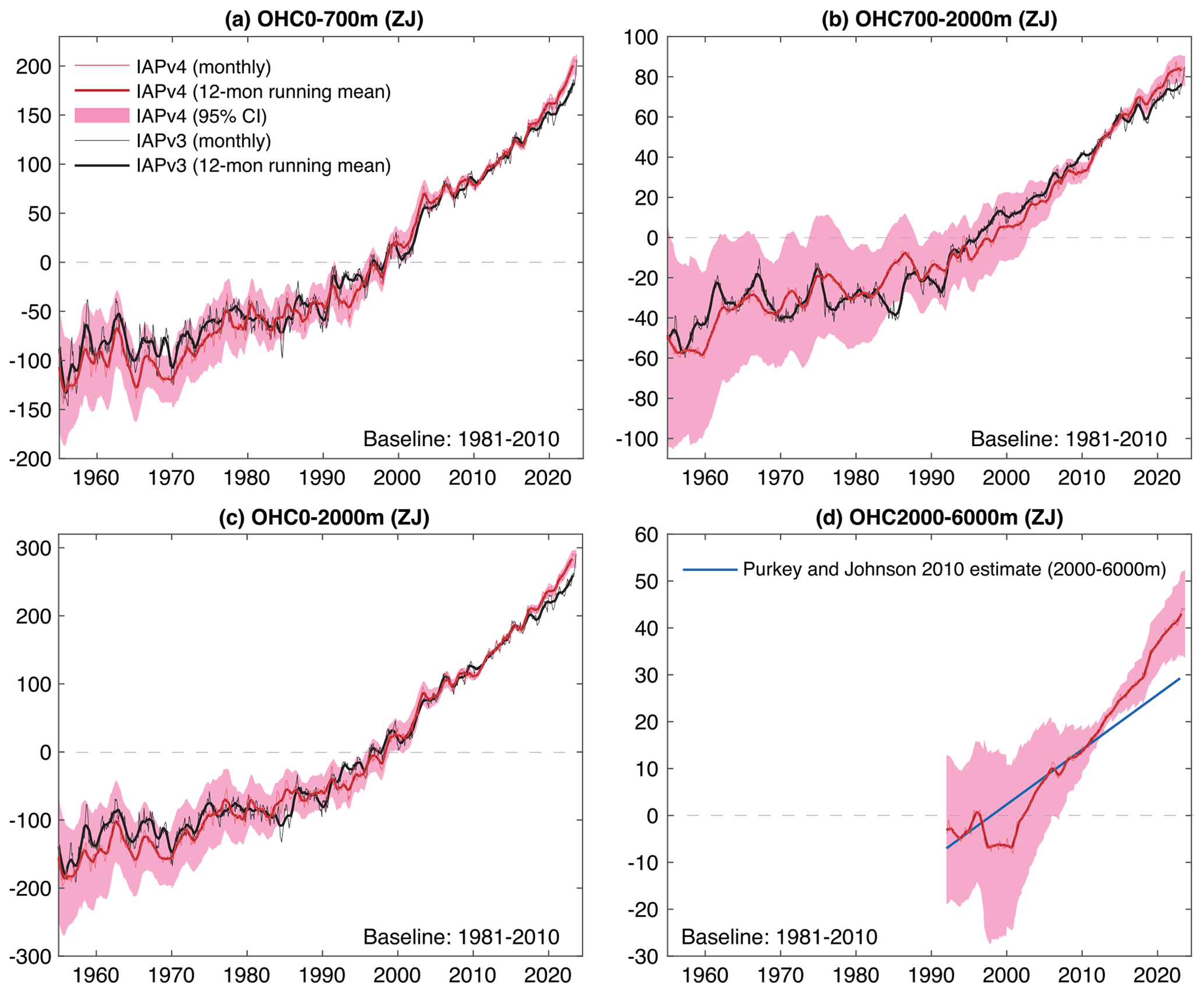
Figure 11Global OHC time series for 0–700 (a), 700–2000 (b), 0–2000 (c), and 2000–6000 m (d). All time series are relative to a 1981–2010 baseline. The shading indicates the 90 % confidence interval. The vertical scales are different for the different panels (ZJ).
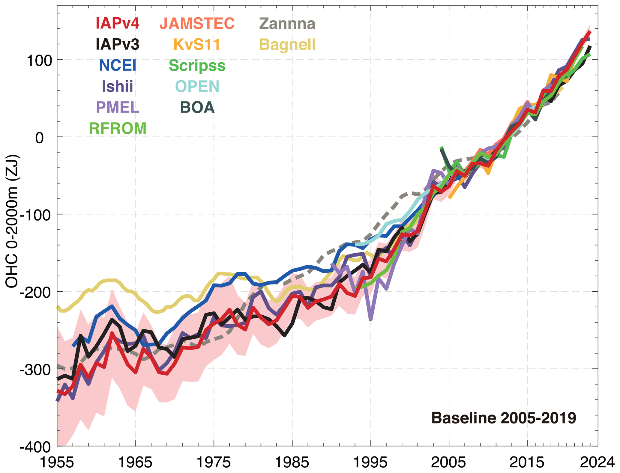
Figure 12A comparison of annual mean 0–2000 m OHC time series from different data products. Solid and dashed lines represent direct and indirect estimates, respectively, and shading indicates the IAPv4 90 % confidence interval (pink shading). OHC anomalies are relative to a 2005–2019 baseline. The plot is updated from Cheng et al. (2022a).
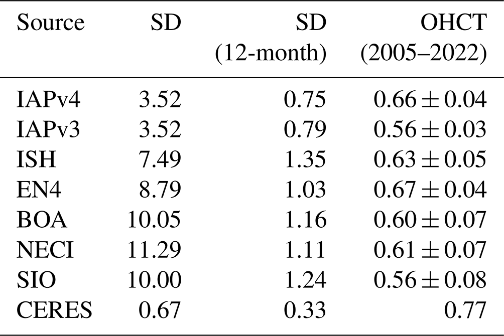
Another feature of IAPv4 is the suppression of month-to-month noise compared to many available data products. Trenberth et al. (2016) noted that the month-to-month variation (quantified by the standard deviation of the monthly dOHC dt time series) in all the in situ OHC records is much larger than implied by the CERES records, suggesting that the OHC variation on this timescale is most likely spurious. Therefore, the magnitude of the month-to-month variation in the OHC record can be used as a benchmark of the data quality. The standard deviation of the CERES record is 0.67 W m−2 from 2005 to 2023 (Loeb et al., 2018), while IAPv4, IAPv3, ISH, EN4, BOA, NCEI, and SIO data show standard deviations of dOHC dt time series of 3.52, 3.52, 7.49, 8.79, 10.05, 11.29, and 10.00 W m−2, respectively, for the upper 2000 m (Table 2). Note that differentiation to get the rate of change amplifies noise, and applying a 12-month running smoother significantly reduces the noise so that the IAPv4 standard deviation becomes 0.75 W m−2, the smallest among the datasets investigated in this study (Table 2) and the most physically plausible time series from this noise level perspective. In addition, the Lyman and Johnson (2013) data suggest a yearly variance ratio of 1.3 between annual RFROM and CERES data from 2008 to 2021. Using the yearly mean OHC trend (OHCT) indicates a ratio of 1.4 in the same period between IAPv4 and CERES, which is similar to that of RFROM.
Table 2Characteristics of the month-to-month variation of the OHCT compared with CERES. Comparisons of different ocean gridded products: the monthly standard deviation (SD) of the monthly rates of change in OHC (W m−2); the corresponding standard deviation of the 12-month running mean (13 points are used, with start points and end points weighted by 0.5); and the linear trend with 90 % confidence limits (W m−2) (global surface area). The values are for 2005–2022. The OHCT for CERES is calculated as the mean of the net TOA radiation flux from 2005 to 2022 multiplied by 0.9, assuming 90 % of the EEI to be stored in the ocean.
3.5 Regional OHC trends
For 1960–2023 (Fig. 13), the IAPv4 trends are slightly lower than IAPv3 in the Pacific Ocean but are slightly higher in the Atlantic Ocean (Fig. 13), with more than 95 % of the ocean area showing a warming trend. The polar regions also show remarkable differences compared to IAPv3 (Sect. 3.1), mainly because of the change in covariance, which improves the spatial reconstruction in the polar regions. IAPv4 shows stronger warming near the boundary current regions, mainly because of the improved QC that does not flag high-temperature anomalies. Nevertheless, the pattern of trends is very similar in the two versions of the data, indicating the robustness of the ocean warming pattern. The Atlantic Ocean (within 50° S–50° N) and the Southern Ocean store more heat than the other basins, which is probably associated with the deep convection and subduction processes effectively transporting heat into the deep layers (Cheng et al., 2022a). The cold spots mainly include the northwestern Pacific and subpolar North Atlantic Ocean. In particular, the so-called “warming hole” in the subpolar North Atlantic Ocean can extend to at least 800 m and is responsible for the decreased OHC in this region. Some studies have linked this fingerprint to the slowdown of the Atlantic Meridional Overturning Circulation (AMOC) (Rahmstorf et al., 2015; Caesar et al., 2018).
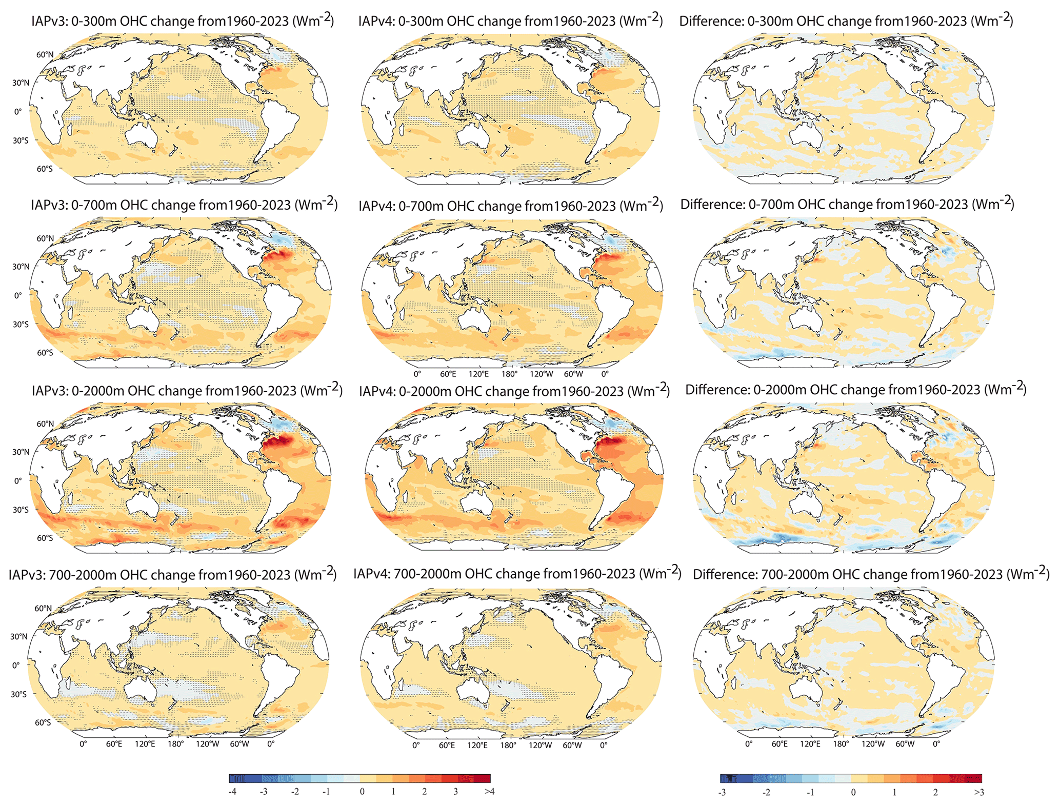
Figure 13Spatial pattern of the OHC trends for 0–300, 0–700, 0–2000 m, and 700–2000 m from 1960 to 2023. The left panels show IAPv3, the middle panels show IAPv4, and the right panels show the differences between IAPv4 and IAPv3.
For 1991–2023 (Fig. 14), the IAPv4 and IAPv3 pattern is also consistent. A trend pattern mimicking a negative Pacific decadal variability (PDV) phase appears in the Pacific for the 0–300, 0–700, and 0–2000 m OHCs. There is a contrast between the warming trend of the tropical western Pacific and the cooling trend of the tropical eastern Pacific. Some studies have linked this pattern to the natural climate mode (PDV) (England et al., 2014), but some suggest that it is a forced change driven by greenhouse gas increases (Fasullo and Nerem, 2018; Mann, 2021). Below 700 m, the 1960–2023 and 1991–2023 trend patterns are similar because deep-ocean warming mainly occurs after 1990. The subtropical western Pacific and southern Indian oceans show cooling, which is likely related to the subtropical gyre intensification but a spin-down in the North Pacific Ocean (Zhang et al., 2014).
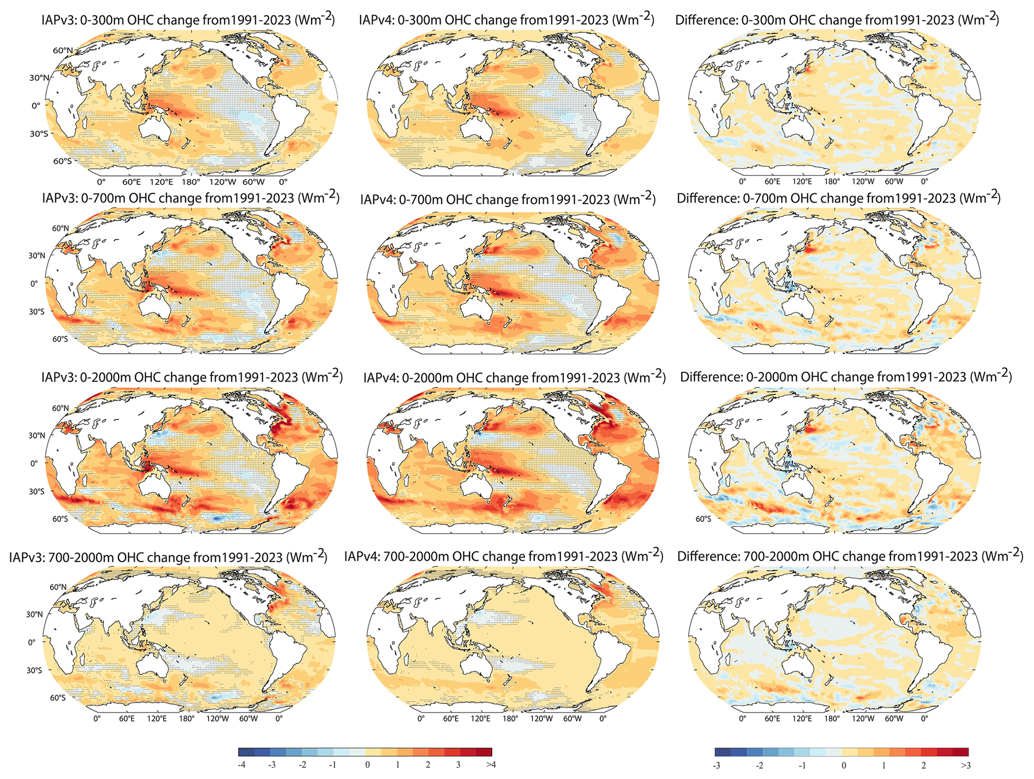
Figure 14Spatial pattern of the OHC trends for 0–300, 0–700, 0–2000, and 700–2000 m from 1991 to 2023. The left panels show IAPv3, the middle panels show IAPv4, and the right panels show the differences between IAPv4 and IAPv3.
Furthermore, the reconstruction of IAPv4 is compared with completely independent observations in the central Labrador Sea (see the Data and methods section for details; Yashayaev, 2007; Yashayaev and Loder, 2017) for the 200–2000 m mean temperature time series (Fig. 15). The direct observations show a substantial decadal variation in the central Labrador Sea, with negative anomalies for 1970–2003 and 2015–2020 and positive anomalies for 1963–1972 and 2004–2014. Reconstructed based on data from the WOD, IAPv4 can represent this decadal variability well. The largest difference occurs in 1989, where direct observations show a nearly zero anomaly, while IAPv4 shows a big negative anomaly. This difference is likely caused by using a time window in IAPv4, which has a smoothing effect on the time series.
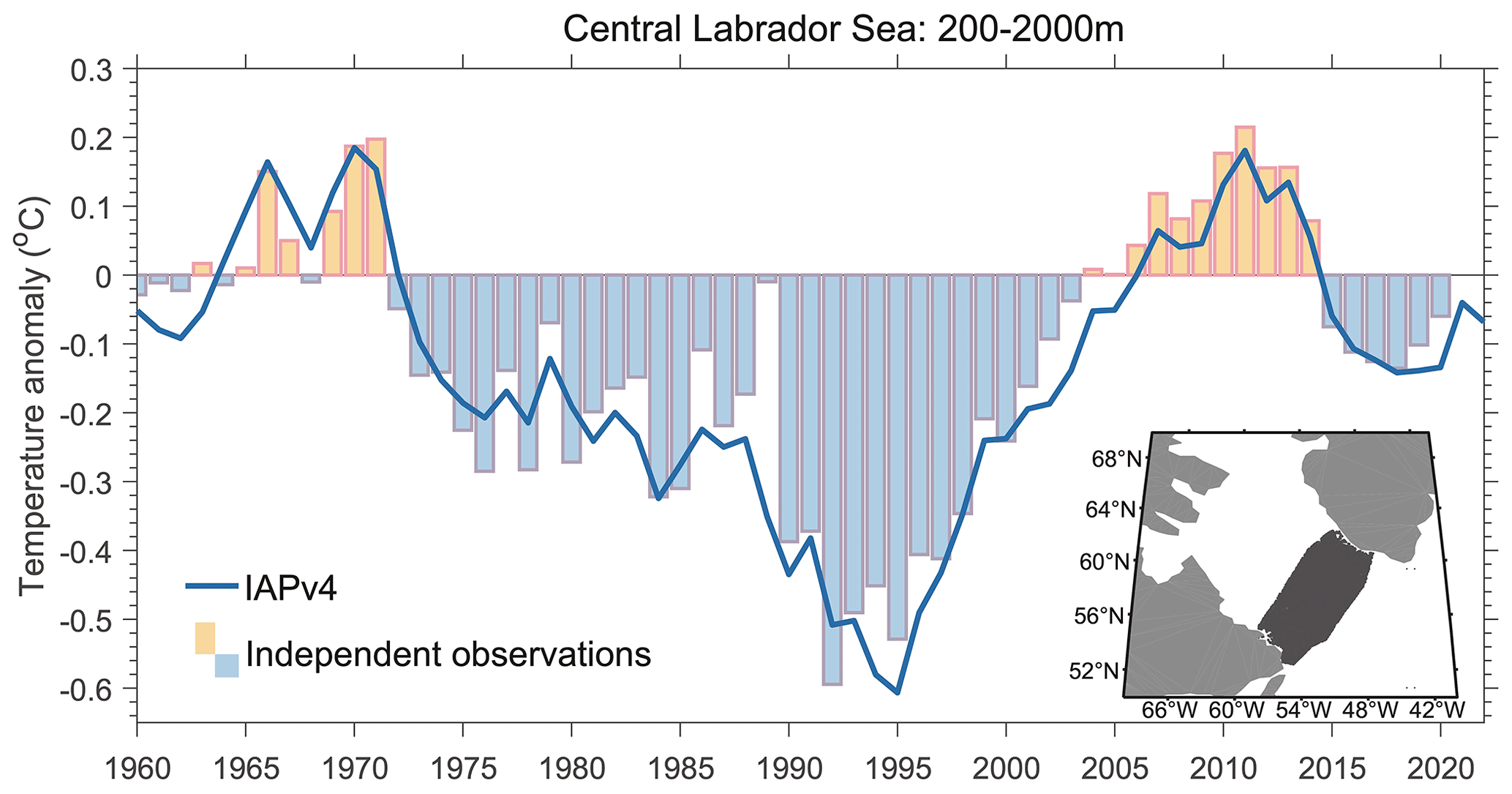
Figure 15Comparison of IAPv4 temperature anomaly data with independent observations in the central Labrador Sea (55–61° N, 304–310° E) from 1960 to 2020. The 200–2000 m averaged temperature anomaly time series is shown, and the baseline is 1960–2020. The inner box shows the locations of the independent observations in black dots (showing a total of 49 849 profiles).
3.6 Ocean meridional heat transport
The ocean meridional heat transport (MHT) is fundamental to maintaining Earth's energy balance. Thus, its change and stability are key to the climate system and its variability. Direct observations of the ocean MHT are conducted only in several cross-basin sections such as RAPID. The ocean MHT can be derived from the OHC and air–sea heat flux data (Trenberth and Fasullo, 2017; Trenberth et al., 2019) as follows: we integrate the OHCT, air–sea heat flux, and heat gain or loss by sea ice changes from the North Pole southward in the Atlantic Ocean and solve the energy budget equation. The residual at each latitude is the MHT, i.e.,
where a is Earth's radius, φ is the latitude, Fs is the net surface heat flux, and Qice is the heat inferred from the changes in sea ice mass. Consistent with Trenberth et al. (2019), this study uses the sea ice volume data from the Pan-Arctic Ice Ocean Modeling and Assimilation System (PIOMAS; Schweiger et al., 2011) and assumes a constant latent heat of fusion of 3.34 × 10⁵ J kg−1 and a density of ice of 900 kg m−3. Both Fs and OHCT are important for the MHT derivation: the integrated air–sea heat flux dominates the magnitude of the MHT, while the OHCT dominates the variability of the MHT (Liu et al., 2020).
The comparison between OHC-derived MHT and RAPID data allows one to check the consistency among the various observations. Here, we calculate the Atlantic MHT from April 2004 to December 2022 using IAPv4 OHC and air–sea net heat flux data (FS) derived from top-of-atmosphere (TOA) net energy flux and atmospheric heat divergence (Fig. 16). FS is an average of three available products, i.e., MAYER2021 (Mayer et al., 2021), TF2018 (Trenberth et al., 2019), and Deep-C Version 5.0 from Reading University (Liu and Allan, 2022; Liu et al., 2020). The data are adjusted following the Trenberth et al. (2019) approach to ensure zero MHT on the Antarctic coast. The inferred time series of MHT at 26.5° N from the other OHC datasets (IAPv3, Ishii, and EN4) are also shown in Fig. 16, compared with the RAPID observations (Johns et al., 2023).
The inferred long-term mean (April 2004–December 2022) MHT from the updated IAPv4 OHCT (solid red line with a mean transport of 1.18 PW) is identical to the RAPID observation of 1.18 ± 0.19 PW. Different OHC datasets cause different interannual variability in the MHT. It is shown that, from 2008 to 2020, the RAPID MHT agrees best with the IAPv4 estimates, with a correlation of 0.52. By comparison, the correlation coefficients between RAPID and IAPv3, EN4, and Ishii are 0.33, 0.51, and 0.49, respectively. Over the entire period of 2005 ∼ 2022, IAPv4 lies mostly within the RAPID uncertainty envelope.
3.7 Interannual variability
The year-to-year variation of OHC is strongly influenced by the El Niño–Southern Oscillation (ENSO) from global to regional scales (Cheng et al., 2019; Roemmich and Gilson, 2011). To demonstrate the change in the OHC-associated ENSO, Fig. 17 shows a Hovmöller diagram of the zonal upper 2000 m OHC and its change (time derivative of OHC: dOHC dt) in the tropical Pacific Ocean from 1985 to 2023, compared with the Oceanic Niño Index (ONI). It is evident that both OHC and OHCT are closely correlated with ENSO.
Before the onset of El Niño events, there is an accumulation of heat (dOHC dt>0) in the southern and equatorial tropical Pacific Ocean region (20° S–5° N). The positive tropical Pacific dOHC dt leads the ONI by ∼ 15 months (with the peak correlation > 0.5), making it a precursor of El Niño (Cane and Zebiak 1985; McPhaden, 2012; Lian et al., 2023). In contrast, heat is redistributed (dOHC dt< 0) from the tropical Pacific (20° S–5° N) to the North Pacific (5–25° N) during and after El Niño (Cheng et al., 2019), with a maximum correlation > 0.8 at 5 months after the El Niño peak. The magnitude of the prominent change can reach up to 50 W m−2 during the 1997–1998 and 2015–2016 extreme El Niño events. For the other moderate El Niño events, the regional Pacific OHC change varies around 10–20 W m−2 (Mayer et al., 2018). This typical heat recharge–discharge paradigm is crucial in ENSO evolution (Jin, 1997). Correspondingly, the zonal OHC anomalies in the Pacific Ocean show a warming state (OHC > 0) between ∼ 20° N and ∼ 5° S before the peak of El Niño events (with the peak correlation >0.7 at 5 months before the El Niño peak), followed by a period of cooling (OHC < 0) after the peak of El Niño (with the peak correlation >0.7 at 12 months after the El Niño peak). These variations are all physically meaningful and indicate that IAPv4 represents regional interannual variability especially associated with ENSO.
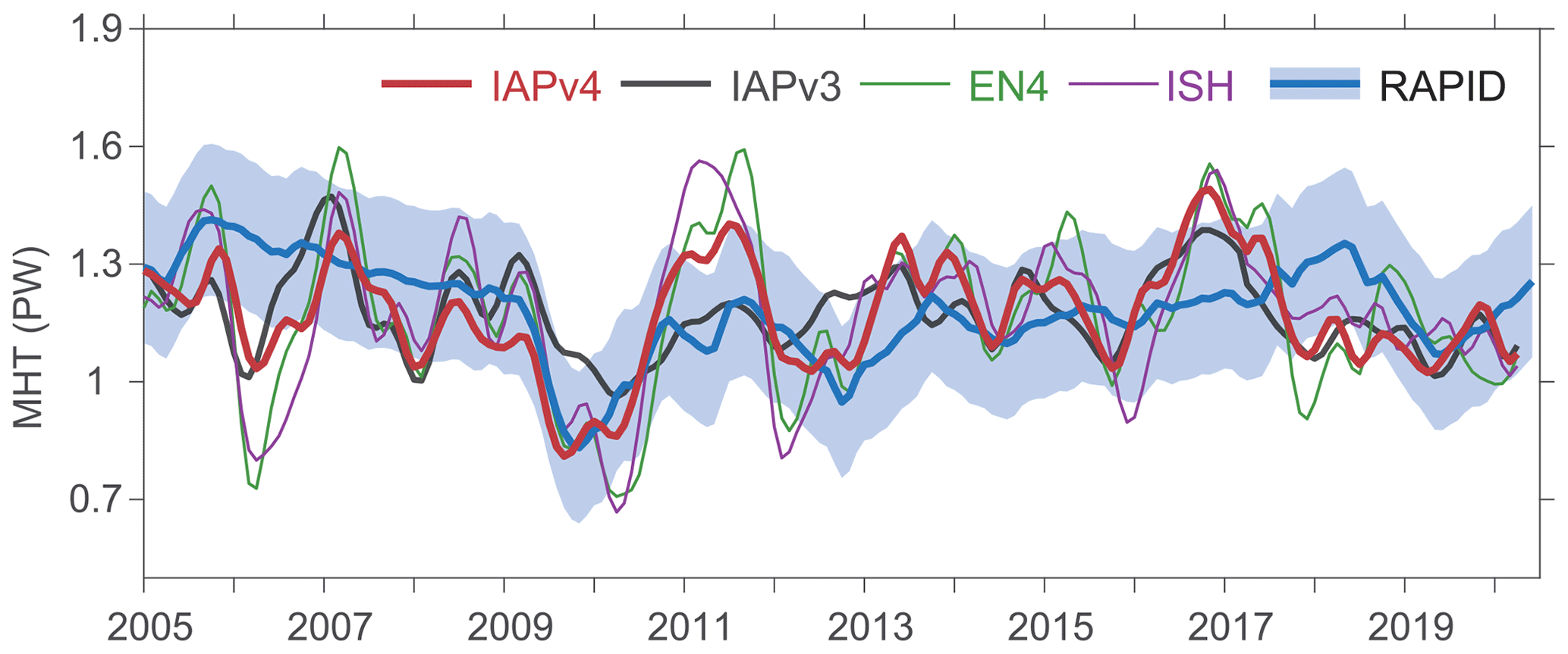
Figure 16Derived meridional heat transport at 26.5° N. The 12-month running mean northward MHT across 26.5° N of the different datasets is compared with the results from the RAPID array (PW). The error bars for RAPID in grey are 1.64σ.
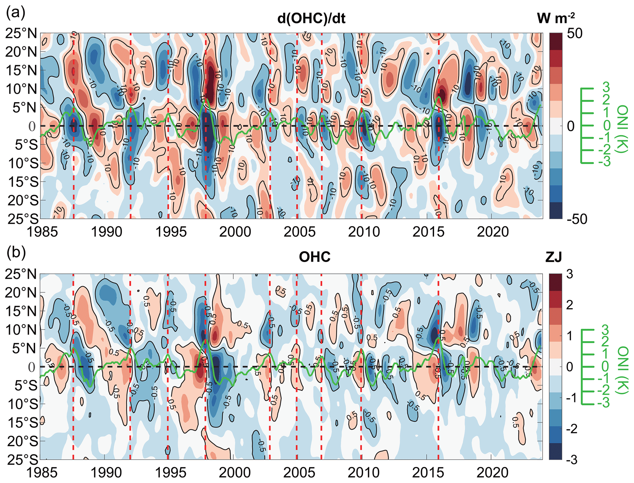
Figure 17Hovmöller diagrams illustrating the zonal mean (a) upper 2000 m dOHC dt (W m−2) and (b) OHC (ZJ) in each 1° latitude band within 25° S ∼ 25° N in the tropical Pacific basin using IAPv4 data. The ONI is shown in green. Vertical dashed lines denote the peak time of each Niño event.
3.8 Ocean and Earth energy budget
The EEI provides a critical quantifier of Earth's energy flow and climate change. It is also policy-relevant because it clearly shows the need to stabilize the climate system. With new T/OHC data, we reassess Earth's energy inventory since 1960. The land, atmosphere, and ice contributions are from the estimates obtained by von Schuckmann et al. (2023) for 1960–2023 and by Trenberth (2022) for 2015–2019.
It is evident that Earth has been accumulating heat since 1960. Earth's heat inventory is 524.0 ± 95.6 ZJ from 1960 to 2023 and 260.3 ± 25.3 ZJ from 2005 to 2023 based on our data. The upper 700 m ocean, 700–2000 m ocean, 2000 m bottom, land, ice, and atmosphere contribute 59.3 %, 24.1 %, 7.4 %, 5.2 %, 2.9 %, and 1.1 %, respectively, of the total EEI since 1960. The relative contribution has changed with time; for instance, since 1993, the contributions are 53.7 % (0–700 m ocean), 24.8 % (700–2000 m ocean), 12.8 % (2000 m–ocean bottom), 4.1 % (land), 3.2 % (ice), and 1.4 % (atmosphere). The land and ice contributions have increased in the last two decades because of accelerated land and sea ice melting (Comiso et al., 2017; Hugonnet et al., 2021; Minière et al., 2024). From 2005 to 2019, more reliable land–atmosphere–ice datasets in Trenberth (2022) suggest a non-ocean contribution of 13.4 ZJ. Combined with the results for OHC with IAPv4, the accumulated EEI is 182.5 ZJ with an ocean heat uptake of 169.1 ± 19.7 for 2005–2019, consistent with the value of 186.4 ± 23.1 ZJ using the non-ocean contribution data from von Schuckmann et al. (2023).
The derived energy inventory has been compared with satellite-based observations at the TOA. Two comparisons are made: (1) integrate the TOA EEI to compare it with the energy inventory (Fig. 18) and (2) take the time derivative of the annual OHC to compare it with the TOA net radiation flux (Fig. 19). Here we always assume that 90 % of the EEI is stored in the ocean and leads to an increase in OHC (Trenberth et al., 2009; Hansen et al., 2011; von Schuckmann et al., 2020; Hakuba et al., 2021).
The first approach avoids calculating the time derivative of OHC, which exacerbates noise in the time series. The net CERES change has been adjusted to 0.71 W m−2 within 2005–2015. Here we adjust the trend of the integrated CERES data to the IAPv4 OHC trend to make it consistent, and then we compare the variability difference (Fig. 18). The root mean square errors (RMSEs) between integrated Deep-C and IAPv4 are 17.9 and 15.5 ZJ between integrated CERES and IAPv4. The comparison also indicates that the heat inventory has a stronger heat increase from 2000 to 2005 but too slow heat accumulation from 2005 to 2010 compared with integrated Deep-C and CERES (Fig. 18). This might be due to the data gaps before the Argo network was fully established. Integrated Deep-C and CERES show stronger heat accumulation since ∼ 2015 than the heat inventory, which is probably associated with the accelerated abyssal ocean warming found by the Deep Argo program (Johnson et al., 2019). Furthermore, IAPv4 OHC shows a slightly higher (but consistent within the uncertainty range) Earth heat uptake compared to the von Schuckmann et al. (2023) results of 76.2 ZJ from 1960 to 2020, mainly because of the correction of Nansen bottle biases and the updates of XBT and MBT biases in IAPv4 data.
The second approach to compare OHC with satellite-based EEI is to calculate the time derivative of OHC. To suppress the month-to-month noises, we estimate annual OHC based on 1-year data centered on June (Fig. 19a) and December (Fig. 19b) separately, and then dOHC dt is calculated with a forward-derivative approach based on the annual time series. The annual mean of the EEI time series is also used here for comparison (Fig. 19). The IAPv4 and CERES estimates show interannual variability with a correlation of 0.44 (the correlation is statistically significant at the 90 % confidence interval, where autocorrelation reduction is taken into account). The higher correlation of IAPv4 versus CERES than IAPv3 increases confidence in the new data (correlation of only ∼ 0.15 for IAPv3). The trend of dOHC dt is 0.36 W m−2 per decade from 2005 to 2023, within the uncertainty range of the CERES record (0.50 ± 0.47 W m−2 per decade in Loeb et al., 2021). However, it should be noted that the calculation of dOHC dt is sensitive to the choices of methods, data products, and time periods because of the noises and variability in the OHC time series. A careful analysis of the trend of dOHC dt (and EEI) is a research priority.
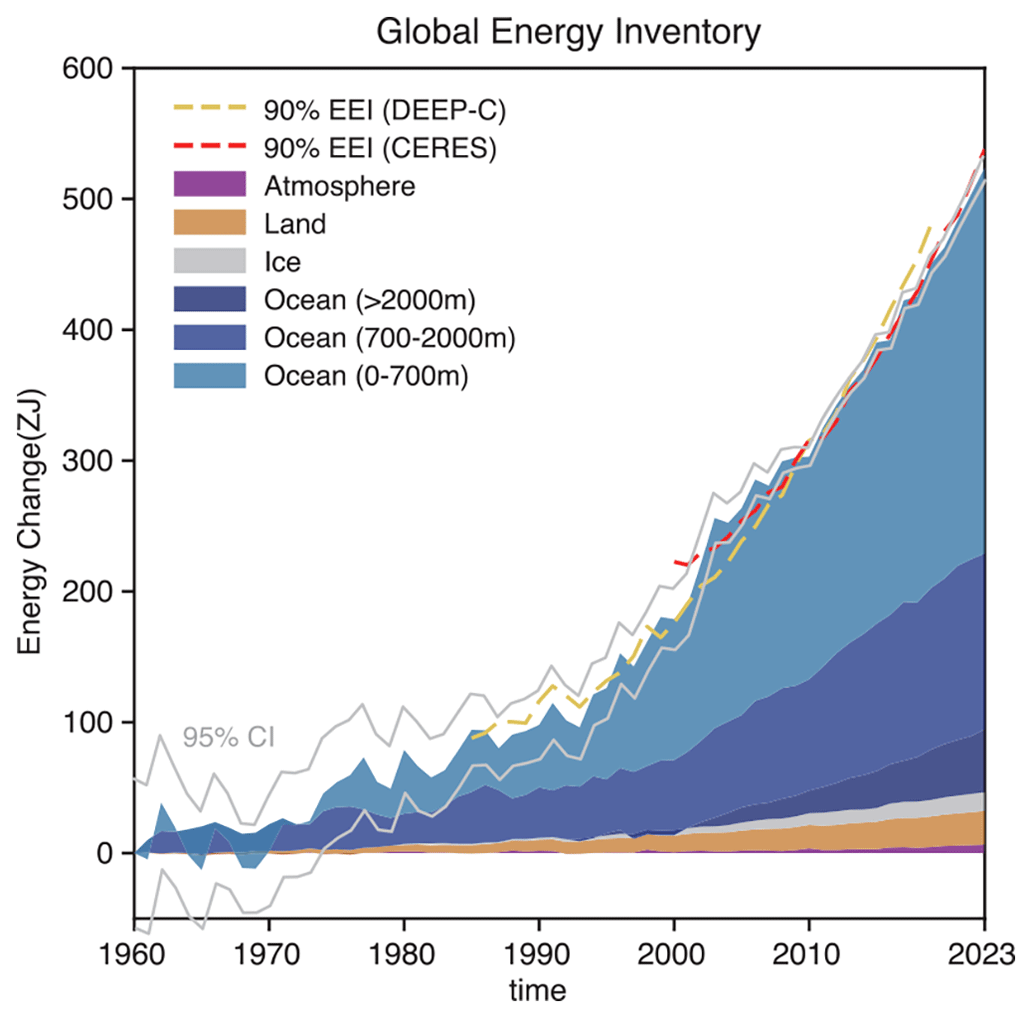
Figure 18The global energy inventory from 1960 to 2023. The atmosphere, land, and ice heat inventory is from von Schuckmann et al. (2023). Integrated EEIs from the Deep-C (1985–2018) (Liu and Allan, 2022) and CERES (2001–2023) (Loeb et al., 2021) datasets are presented with dashed lines for comparison, with the trend adjusted to the IAP estimate to account for the arbitrary choice of integration constant. The 95 % confidence interval is presented assuming the independency of different budget components.
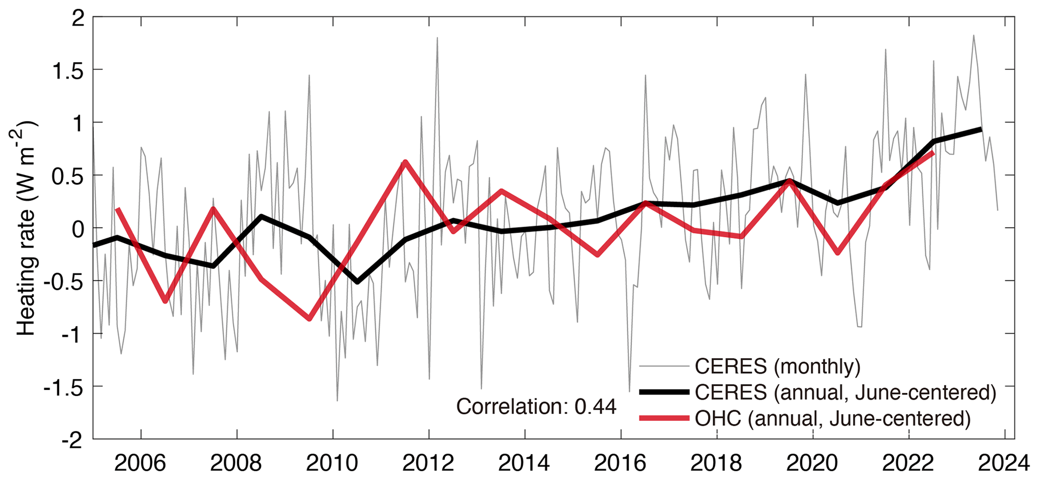
Figure 19Annual ocean heating rate (derived from IAPv4 data, in red) compared with CERES data (grey line for monthly data, black line for annual mean data). Both annual OHC and CERES EEI data are centered on June. The long-term mean is removed for all the time series.
3.9 Steric sea level and sea level budget
The updated IAPv4 data are used to assess the sea level budget for 1960–2023 in combination with the other data, including IAP salinity data, glaciers, and Greenland and Antarctic ice sheet mass loss from Frederikse et al. (2020) and the altimetry sea level record (see the Data and methods section for details). From 1960 to 2023, the observed global mean sea level (GMSL) rise was 2.07 ± 0.55 mm yr−1 (Frederikse et al., 2020), which was derived by combining tide gauge observations with estimates of local vertical land motion from permanent Global Positioning System stations and the difference between tide gauge and satellite altimetry observations (Frederikse et al., 2018). During the same period, the sum of the contributors (glaciers, Greenland and Antarctic ice sheets, land water storage, and steric sea level) yields a mean sea level rise of 1.87 ± 0.42 mm yr−1. Thus, the sea level budget can be closed within a 90 % confidence interval. This updated estimate indicates that the steric sea level, Antarctic ice sheet, Greenland ice sheet, glaciers, and land water storage contribute to the total sea level with 47.3 %, 8.6 %, 18.0 %, 29.1 %, and −3.1 %, respectively, for 1960–2023.
To isolate the contribution of IAPv4 to the sea level budget, we replace the steric sea level estimate in Frederikse et al. (2020) with IAPv4 and reassess the sea level budget for 1960–2018, 1993–2018, and 2005–2018, and the other components are identical to Frederikse et al. (2020). Two metrics are used to quantify the performance of the sea level budget closure: the mean residual error and the temporal RMSE between the observed GMSL and the sum of the contributions. We find that the residual sea level budgets based on IAPv4 are 0.20 ± 0.53, 0.11 ± 0.34, and 0.47 ± 0.56 mm yr−1 for 1960–2018, 1993–2018, and 2005–2018, respectively. These mean residual errors are all smaller than presented in Frederikse et al. (2020), which showed residual errors of 0.29 ± 0.57, 0.20 ± 0.34, and 0.54 ± 0.58 mm yr−1 for 1960–2018, 1993–2018, and 2005–2018, respectively. The RMSEs using IAPv4 (or using the steric sea level in Frederikse et al., 2020) are 5.59 (5.35), 4.89 (5.33), and 4.21 (4.51) mm, respectively, for the three abovementioned periods. Therefore, both metrics show that IAPv4 data improve the sea level budget in three typical periods.
A similar test is done with the IPCC-AR6 sea level budget estimate (Gulev et al., 2021): the thermosteric sea level estimate in IPCC-AR6 is replaced with IAPv4, and the sea level budget is reassessed for 1993–2018. IAPv4 suggests a larger thermosteric sea level rise of 1.43 ± 0.16 for 1993–2018 than the IPCC (1.31 ± 0.36 mm yr−1) from 1993 to 2018. Replacing the thermosteric sea level estimate with IAPv4 reduces the mean residual error from 0.40 ± 0.57 to 0.28 ± 0.48 mm yr−1. This suggests that the stronger warming since 1993 revealed by IAPv4 than assessed in IPCC-AR6 (Gulve et al., 2021) seems more realistic.
After 2002, the GRACE satellite supported the direct observation of the barystatic sea level, which is the sum of the sea level change due to the land water storage, the Antarctic ice sheet, the Greenland ice sheet, and glaciers. The sea level budget can be obtained by comparing altimetry-based GMSL with the barystatic sea level observed by GRACE and the steric sea level. It is evident that the sea level budget can be closed between 2002 and 2015 with ± 5 mm residual errors (Fig. 20b). However, after ∼ 2015, the sum of the steric and barystatic sea levels is smaller than the total sea level rise for all ocean temperature products. Previous studies attributed this misclosure to salinity data biases (Barnoud et al., 2021), altimetry data errors (Barnoud et al., 2023), and GRACE data errors (Wang et al., 2021). The steric sea level inferred from IAPv4 showed a lower residual (∼ 5 mm) between 2005 and 2023 than ISH and EN4 data (10∼ 20 mm), indicating that the temperature data might be partly responsible for lack of closure of the sea level budget since ∼ 2015. This suggests again that the stronger warming in recent years, as indicated by IAPv4, is more realistic. As discussed in Sect. 3.4, the QC is mainly responsible for the increased warming of IAPv4 compared with IAPv3 since ∼ 2015 (Fig. 11).
Many traditional QC procedures use a static climatological range check to filter out outliers, which does not account for the increase in extreme events with climate change and removes too many extreme (positive) values during the recent period. Thus, we strongly recommend that data product generation groups revisit the QC procedure. Furthermore, as the stronger long-term OHC trends since ∼ 1960 in IAPv4 than in IAPv3 are mainly attributed to the bias corrections for Nansen bottle, MBT, and XBT data, it is also recommended that international groups revisit the biases in ocean observations.
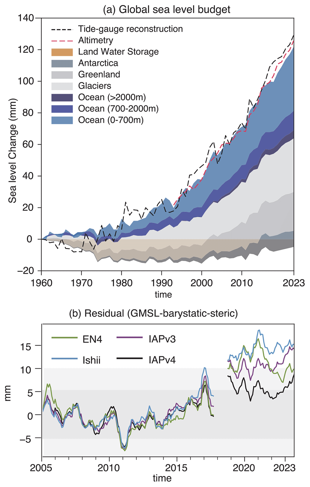
Figure 20(a) The sea level budget from 1960 to 2023: observed GMSL for 1960–2023 and the individual contributions from land water storage, Antarctica, Greenland, and glaciers (Frederikse et al., 2020). The budget is relative to a 1960 baseline. Here, the land water storage and glacier data are through 2018, and a linear extrapolation is made for 2019–2023. Antarctic ice sheet and Greenland ice sheet changes are estimated by GRACE after 2018. Tide gauges after 2018 are updated by altimetry. The altimetry sea level is shown in red dashed line for comparison. (b) Sea level budget residual time series since 2005: the residual of the GMSL minus the barystatic and steric sea level. The seasonal cycle is reduced based on the 2005–2015 climatology. Six-month running means are shown here to reduce the noise.
The IAPv4 global ocean temperature product is available at https://doi.org/10.12157/IOCAS.20240117.002 (Cheng et al., 2024a) and http://www.ocean.iap.ac.cn/, last access: 1 May 2024.
The IAPv4 global ocean heat content product is available at https://doi.org/10.12157/IOCAS.20240117.001 (Cheng et al., 2024b) and http://www.ocean.iap.ac.cn/.
The code used in this paper includes data quality control bias corrections, and the resultant dataset is available at http://www.ocean.iap.ac.cn/.
The data used in this study (but not generated by this work) are listed below. The IAP data are available at http://www.ocean.iap.ac.cn/. The NCEI/NOAA data are available at https://www.ncei.noaa.gov/products/ (Levitus et al., 2012, NOAA National Centers for Environmental Information, last access: 15 May 2024). The ISH data are available at https://www.data.jma.go.jp/gmd/kaiyou/english/ohc/ohc_global_en.html (Ishii et al., 2017, last access: 10 May 2024). The EN4 data are available at https://www.metoffice.gov.uk/hadobs/en4/index.html (Good et al., 2013; last access: 10 May 2024). For SSTs, there are ERSSTv5 (https://www1.ncdc.noaa.gov/pub/data/cmb/ersst/v5/netcdf/, Huang et al., 2017, last access: 10 January 2024), COBE2 (https://psl.noaa.gov/data/gridded/data.cobe2.html, Hirahara et al., 2014, last access: 10 January 2014), and HadISST (https://www.metoffice.gov.uk/hadobs/hadisst/, Rayner et al., 2003, last access: 10 January 2024). For sea level data, there are AVISO + GMSL (https://www.aviso.altimetry.fr/en/data/, last access: 10 July 2023), JPL GRACE (https://grace.jpl.nasa.gov/data/get-data/jpl_global_mascons/, Watkins et al., 2015, last access: 3 August 2023), and Frederikse et al. (2020) (https://zenodo.org/records/3862995, last access: 2 February 2023). The data in von Schuckmann et al. (2023) are available at https://www.wdc-climate.de/ui/entry?acronym=GCOS_EHI_1960-2020 (von Schuckmann et al., 2022; last access: 2 February 2023). Argo data were collected and made freely available by the International Argo Program and the national programs that contribute to it (https://argo.ucsd.edu, https://www.ocean-ops.org, Argo, 2000; last access: 1 December 2023). DEEP-C data are available at https://doi.org/10.17864/1947.000347 (Liu and Allan, 2022; last access: 20 April 2024). CERES data are available at https://asdc.larc.nasa.gov/project/CERES (Loeb et al., 2021; last access: 20 April 2024). GIOMAS ice volume data are available at https://psc.apl.washington.edu/zhang/Global_seaice/data.html (Zhang and Rothrock, 2003; last access: 20 April 2024). SCRIPPS data are available at http://sio-argo.ucsd.edu/RG_Climatology.html (Roemmich and Gilson, 2009; last access: 10 May 2024). BOA data are available at https://argo.ucsd.edu/data/argo-data-products/ (Li et al., 2017; last access: 10 May 2024).
This paper introduces a new version of the ocean temperature and ocean heat content gridded products and describes the data source and data processing techniques in detail. The key technical advances include the new QC, new or updated XBT/MBT/bottle/APB bias corrections, a new ocean temperature climatology, an improved mapping approach, and grid cell ocean volume corrections. These data and technical advances allow a better estimate of long-term ocean temperature and heat content changes since the mid-1950s from the sea surface down to 2000 m. We show that the new data product could better close the sea level and energy budgets than IAPv3. For rates of change, compared with CERES, IAPv4 also shows a better correlation from 2005 to 2023 than IAPv3.
Despite several marked improvements, issues needing further investigation remain. First, although interannual and decadal-scale changes in satellite-based EEI and observational OHC are generally consistent, a mismatch remains between EEI and OHC for their month-to-month variation, as the monthly variation of OHC is still much larger than implied by EEI. There are several possibilities, in our opinion: first, there is substantial monthly heat storage and release for land and ice, which needs to be accurately quantified; second, the accuracy of OHC estimates on a monthly basis still needs to be improved for month-to-month variation because of the limited data coverage; and third, the EEI observed by CERES also suffers from sampling biases on a monthly basis (Loeb et al., 2009). Thus, a better understanding of the monthly variation of OHC and EEI is still a research priority. Besides, the failure to close the 2015–2023 sea level budget indicates that the underlying data still have bias problems that need to be explored and resolved.
Second, the application of CODC-QC in IAPv4 leads to a stronger ocean warming rate in the past decade than WOD-QC in IAPv3 because WOD-QC removes more positive temperature anomalies than CODC-QC. This could imply that the rate of increase in OHC is still slightly underestimated and deserves an in-depth investigation. Several fundamental questions must be answered: first, are there still real temperature extremes being removed by CODC-QC, such as in small warm or cold eddies? Are the extremes well sampled by the current observation system? If not, what is the impact? Moreover, it is clear that the high latitudes where sea ice occurs are not well sampled and need more attention.
Third, during the development of the data product, we discovered that many metadata related to the profiles in the WOD are missing and that many existing metadata are incorrect, also giving rise to duplicate profiles and putting a strain on the overall quality of a database of oceanic observations. More than ever, long-term concerted efforts are needed to eliminate duplicate profiles and identify and correct missing metadata using statistical methods, expert control, or machine learning techniques. For example, the International Quality-Controlled Ocean Database (IQuOD) group is coordinating some activities related to data processing techniques, uncertainty quantification, and improvement of the overall quality of ocean data (Cowley et al., 2021).
Fourth, the deep-ocean changes below 2000 m are estimated based on the currently available data, including data from hydrological sections and Deep Argo. The IAP mapping technique is applied. Because of the lack of independent observations with global ocean coverage, evaluating the deep-ocean change estimate is still dicey. Thus, the below-2000 m estimate should be used with caution, as also indicated in previous estimates (Purkey and Johnson, 2010; Desbruyères et al., 2017; Good et al., 2013). A community-agreed evaluation approach for the deep-ocean changes is critically needed. Other mapping techniques deserving further investigation include interpolation on isopycnal surfaces (Palmer and Haines, 2009).
Furthermore, the quantification of uncertainty for in situ measurements, gridded T/OHC values, and the global OHC estimates needs to be improved. IAPv4 only accounts for the instrumental error and the sampling or mapping error. In the future, comprehensive quantification of other uncertainty sources will be made, including the choice of climatology, vertical interpolation, or XBT/MBT/APB/bottle corrections. It is also necessary to analyze the correlation between these error sources. This also helps us to understand regions with larger uncertainty for OHC estimates, which supports the design of the global ocean observing system.
The supplement related to this article is available online at: https://doi.org/10.5194/essd-16-3517-2024-supplement.
LC worked on this study's conceptualization, coordination, methodologies, and manuscript writing. ZT worked on in situ observation collections, the metadata format, and the automated quality control procedure (CODC-QC) development. YP worked on calculating and comparing the OHC's annual cycle, the mixed layer depth, and the MHTs among the different datasets. VG worked on bias correction schemes for MBT, APB, and bottle data and on developing the automated quality control procedure. HY worked on the analysis of the interannual variability. JD worked on the OHC trend calculation and analysis. GL worked on the SST calculation and its analysis. HZ worked on the global energy and sea level budget calculations and analyses. YL and YJ worked on the volume correction. All the authors contributed to the formal analysis, data validation, and editing of the original draft.
The contact author has declared that none of the authors has any competing interests.
Publisher's note: Copernicus Publications remains neutral with regard to jurisdictional claims made in the text, published maps, institutional affiliations, or any other geographical representation in this paper. While Copernicus Publications makes every effort to include appropriate place names, the final responsibility lies with the authors.
The calculations in this study were carried out on the ORISE Supercomputer and National Key Scientific and Technological Infrastructure project “Earth System Science Numerical Simulator Facility” (EarthLab). Some data were collected on board R/V Shiyan 6, implementing the Open Research Cruise NORC2022-10+NORC2022-303 supported by NSFC Shiptime Sharing Projects 42149910. NCAR is sponsored by the US National Science Foundation. We acknowledge the World Climate Research Programme's Working Group on Coupled Modelling, which is responsible for CMIP, and we thank the climate modeling groups for producing and making their model output available through the Earth System Grid Federation. The Argo program is part of the Global Ocean Observing System.
The IAP/CAS analysis is supported by the National Natural Science Foundation of China (grant nos. 42122046, 42076202, 42206208, and 42261134536), the Strategic Priority Research Program of the Chinese Academy of Sciences (grant no. XDB42040402), the new Cornerstone Science Foundation through the XPLORER PRIZE, the DAMO Academy Young Fellow, Youth Innovation Promotion Association, the Chinese Academy of Sciences, and the Young Talent Support Project of the Guangzhou Association for Science and Technology.
This paper was edited by Davide Bonaldo and reviewed by Michael Mayer and Armin Koehl.
Abraham, J. P. and Cheng, L.: Intersection of Climate Change, Energy, and Adaptation, Energies, 15, 5886, https://doi.org/10.3390/en15165886, 2022.
Abraham, J. P., Baringer, M., Bindoff, N. L., Boyer, T., Cheng, L. J., Church, J. A., Conroy, J. L., Domingues, C. M., Fasullo, J. T., Gilson, J., Goni, G., Good, S. A., Gorman, J. M., Gouretski, V., Ishii, M., Johnson, G. C., Kizu, S., Lyman, J. M., Macdonald, A. M., Minkowycz, W. J., Moffitt, S. E., Palmer, M. D., Piola, A. R., Reseghetti, F., Schuckmann, K., Trenberth, K. E., Velicogna, I., and Willis, J. K.: A review of global ocean temperature observations: Implications for ocean heat content estimates and climate change, Rev. Geophys., 51, 450–483, https://doi.org/10.1002/rog.20022, 2013.
Abraham, J. P., Cheng, L., Mann, M. E., Trenberth, K., and von Schuckmann, K.: The ocean response to climate change guides both adaptation and mitigation efforts, Atmos. Ocean. Sci. Lett., 15, 100221, https://doi.org/10.1016/j.aosl.2022.100221, 2022.
Argo: Argo float data and metadata from Global Data Assembly Centre (Argo GDAC), SEANOE [data set], https://doi.org/10.17882/42182, 2000.
Bagnell, A. and DeVries, T.: 20(th) century cooling of the deep ocean contributed to delayed acceleration of Eart”s energy imbalance, Nat. Commun., 12, 4604, https://doi.org/10.1038/s41467-021-24472-3, 2021.
Barker, P. M. and McDougall, T. J.: Two Interpolation Methods Using Multiply-Rotated Piecewise Cubic Hermite Interpolating Polynomials, J. Atmos. Ocean Technol., 37, 605–619, https://doi.org/10.1175/JTECH-D-19-0211.1, 2020.
Barnoud, A., Pfeffer, J., Guérou, A., Frery, M.-L., Siméon, M., Cazenave, A., Chen, J., Llovel, W., Thierry, V., Legeais, J.-F., and Ablain, M.: Contributions of Altimetry and Argo to Non-Closure of the Global Mean Sea Level Budget Since 2016, Geophys. Res. Lett., 48, e2021GL092824, https://doi.org/10.1029/2021GL092824, 2021.
Barnoud, A., Pfeffer, J., Cazenave, A., Fraudeau, R., Rousseau, V., and Ablain, M.: Revisiting the global mean ocean mass budget over 2005–2020, Ocean Sci., 19, 321–334, https://doi.org/10.5194/os-19-321-2023, 2023.
Bindoff, N. L., Cheung, W. W. L., Kairo, J. G., Arístegui, J., Guinder, V. A., Hallberg, R., Hilmi, N., Jiao, N., and Karim, M. S.: Changing Ocean, Marine Ecosystems, and Dependent Communities, in: IPCC Special Report on the Ocean and Cryosphere in a Changing Climate, edited by: Pörtner, H.-O., Roberts, D. C., Masson-Delmotte, V., Zhai, P., Tignor, M., Poloczanska, E., Mintenbeck, K., Alegría, A., Nicolai, M., Okem, A., Petzold, J., Rama, B., and Weyer, N. M., Cambridge University Press, Cambridge, UK and New York, NY, USA, 447–587, https://doi.org/10.1017/9781009157964.007, 2019.
Boyer, T., Domingues, C. M., Good, S. A., Johnson, G. C., Lyman, J. M., Ishii, M., Gouretski, V., Willis, J. K., Antonov, J., Wijffels, S., Church, J. A., Cowley, R., and Bindoff, N. L.: Sensitivity of Global Upper Ocean Heat Content Estimates to Mapping Methods, XBT Bias Corrections, and Baseline Climatologies, J. Clim., 29, 4817–4842, https://doi.org/10.1175/JCLI-D-15-0801.1, 2016.
Caesar, L., Rahmstorf, S., Robinson, A., Feulner, G., and Saba, V.: Observed fingerprint of a weakening Atlantic Ocean overturning circulation, Nature, 556, 191–196, https://doi.org/10.1038/s41586-018-0006-5, 2018.
Cane, M. A. and Zebiak, S. E.: A theory for El Niño and the southern oscillation, Science, 228, 1085–1087, https://doi.org/10.1126/science.228.4703.1085, 1985.
Cheng, L.: Sensitivity of Ocean Heat Content to Various Instrumental Platforms in Global Ocean Observing System, Ocean-Land-Atmos. Res., 3, 0037, https://doi.org/10.34133/olar.0037, 2024a.
Cheng, L. and Zhu, J.: Uncertainties of the Ocean Heat Content Estimation Induced by Insufficient Vertical Resolution of Historical Ocean Subsurface Observations, J. Atmos. Ocean Technol., 31, 1383–1396, https://doi.org/10.1175/JTECH-D-13-00220.1, 2014.
Cheng, L. and Zhu, J.: Influences of the Choice of Climatology on Ocean Heat Content Estimation, J. Atmos. Ocean Technol., 32, 388–394, https://doi.org/10.1175/JTECH-D-14-00169.1, 2015.
Cheng, L. and Zhu, J.: Benefits of CMIP5 Multimodel Ensemble in Reconstructing Historical Ocean Subsurface Temperature Variations, J. Clim., 29, 5393–5416, https://doi.org/10.1175/JCLI-D-15-0730.1, 2016.
Cheng, L., Zhu, J., Cowley, R., Boyer, T., and Wijffels, S.: Time, Probe Type, and Temperature Variable Bias Corrections to Historical Expendable Bathythermograph Observations, J. Atmos. Ocean. Technol., 31, 1793–1825, https://doi.org/10.1175/jtech-d-13-00197.1, 2014.
Cheng, L., Abraham, J., Goni, G., Boyer, T., Wijffels, S., Cowley, R., Gouretski, V., Reseghetti, F., Kizu, S., Dong, S., Bringas, F., Goes, M., Houpert, L., Sprintall, J., and Zhu, J.: XBT Science: Assessment of Instrumental Biases and Errors, B. Am. Meteorol. Soc., 97, 924–933, https://doi.org/10.1175/BAMS-D-15-00031.1, 2016.
Cheng, L., Trenberth, K. E., Fasullo, J., Boyer, T., Abraham, J., and Zhu, J.: Improved estimates of ocean heat content from 1960 to 2015, Sci. Adv., 3, e1601545, https://doi.org/10.1126/sciadv.1601545, 2017.
Cheng, L., Luo, H., Boyer, T., Cowley, R.. Abraham, J., Gouretski, V., Reseghetti, F., and Zhu, J.: How Well Can We Correct Systematic Errors in Historical XBT Data?, J. Atmos. Ocean. Technol., 35, 1103–1125, https://doi.org/10.1175/JTECH-D-17-0122.1, 2018.
Cheng, L., Trenberth, K. E., Fasullo, J. T., Mayer, M., Balmaseda, M., and Zhu, J.: Evolution of Ocean Heat Content Related to ENSO, J. Clim., 32, 3529–3556, https://doi.org/10.1175/jcli-d-18-0607.1, 2019.
Cheng, L., Trenberth, K. E., Gruber, N., Abraham, J. P., Fasullo, J. T., Li, G., Mann, M. E., Zhao, X., and Zhu, J.: Improved Estimates of Changes in Upper Ocean Salinity and the Hydrological Cycle, J. Clim., 33, 10357–10381, https://doi.org/10.1175/JCLI-D-20-0366.1, 2020.
Cheng, L., von Schuckmann, K., Abraham, J. P., Trenberth, K. E., Mann, M. E., Zanna, L., England, M. H., Zika, J. D., Fasullo, J. T., Yu, Y., Pan, Y., Zhu, J., Newsom, E. R., Bronselaer, B., and Lin, X.: Past and future ocean warming, Nat. Rev. Earth Environ., 3, 776–794, https://doi.org/10.1038/s43017-022-00345-1, 2022a.
Cheng, L., Foster, G., Hausfather, Z., Trenberth, K. E., and Abraham, J.: Improved quantification of the rate of ocean warming, J. Clim., 35, 4827–4840, https://doi.org/10.1175/jcli-d-20-0366.1, 2022b.
Cheng, L., Tan, Z., Pan, Y., Zheng, H., Zhu, Y., Wei, W., Du, J., Li, G., Ye, H., Gourteski, V.: IAP temperature 1° gridded analysis product (IAPv4), CODC [data set], https://doi.org/10.12157/IOCAS.20240117.002, 2024a.
Cheng, L., Tan, Z., Pan, Y., Zheng, H., Zhu, Y., Wei, W., Du, J., Li, G., Ye, H., and Gourteski, V.: IAP global ocean heat content 1° gridded analysis product (IAPv4), CODC [data set], https://doi.org/10.12157/IOCAS.20240117.001, 2024b.
Chu, P. C. and Fan, C.: Global climatological data of ocean thermohaline parameters derived from WOA18, Sci. Data, 10, 408, https://doi.org/10.1038/s41597-023-02308-7, 2023.
Comiso, J. C., Meier, W. N., and Gersten, R.: Variability and trends in the Arctic Sea ice cover: Results from different techniques, J. Geophys. Res.-Ocean., 122, 6883–6900, https://doi.org/10.1002/2017JC012768, 2017.
Cowley, R., Killick, R. E., Boyer, T., Gouretski, V., Reseghetti, F., Kizu, S., Palmer, M. D., Cheng, L., Storto, A., Le Menn, M., Simoncelli, S., Macdonald, A. M., and Domingues, C. M.: International Quality-Controlled Ocean Database (iQuOD) v0.1: The Temperature Uncertainty Specification, Front. Mar. Sci., 8, 689695, https://doi.org/10.3389/fmars.2021.689695, 2021.
Dangendorf, S., Frederikse, T., Chafik, L., Klinck, J. M., Ezer, T., and Hamlington, B. D.: Data-driven reconstruction reveals large-scale ocean circulation control on coastal sea level, Nat. Clim. Change, 11, 514–520, https://doi.org/10.1038/s41558-021-01046-1, 2021.
de Boyer Montégut, C., Madec, G., Fischer, A. S., Lazar, A., and Iudicone, D.: Mixed layer depth over the global ocean: An examination of profile data and a profile-based climatology, J. Geophys. Res.-Ocean., 109, C12003, https://doi.org/10.1029/2004JC002378, 2004.
Desbruyères, D., McDonagh, E. L., King, B. A., and Thierry, V.: Global and full-depth ocean temperature trends during the early twenty-first century from Argo and repeat hydrography, J. Clim., 30, 1985–1997, 2017.
England, M. H., McGregor, S., Spence, P., Meehl, G. A., Timmermann, A., Cai, W., Gupta, A. S., McPhaden, M. J., Purich, A., and Santoso, A.: Recent intensification of wind-driven circulation in the Pacific and the ongoing warming hiatus, Nat. Clim. Change, 4, 222–227, https://doi.org/10.1038/nclimate2106, 2014.
Fasullo, J. T. and Nerem, R. S.: Altimeter-era emergence of the patterns of forced sea-level rise in climate models and implications for the future, P. Natl. Acad. Sci. USA, 115, 12944–12949, https://doi.org/10.1073/pnas.1813233115, 2018.
Frederikse, T., Jevrejeva, S., Riva, R. E. M., and Dangendorf, S.: A Consistent Sea-Level Reconstruction and Its Budget on Basin and Global Scales over 1958–2014, J. Clim., 31, 1267–1280, https://doi.org/10.1175/JCLI-D-17-0502.1, 2018.
Frederikse, T., Landerer, F., Caron, L., Adhikari, S., Parkes, D., Humphrey, V. W., Dangendorf, S., Hogarth, P., Zanna, L., Cheng, L., and Wu, Y.-H.: The causes of sea level rise since 1900, Nature, 584, 393–397, https://doi.org/10.1038/s41586-020-2591-3, 2020 (data set available at https://zenodo.org/records/3862995).
Garcia, H. E., Boyer, T. P., Locarnini, R. A., Baranova, O. K., and Zweng, M. M.: World Ocean Database 2018: User's Manual, T. E. A. V. Mishonov, MD NOAA Atlas NESDIS 87, NOAA, Silver Spring, 2018
Goni, G. J., Sprintall, J., Bringas, F., Cheng, L., Cirano, M., Dong, S., Domingues, R., Goes, M., Lopez, H., Morrow, R., Rivero, U., Rossby, T., Todd, R. E., Trinanes, J., Zilberman, N., Baringer, M., Boyer, T., Cowley, R., Domingues, Hutchinson, K., Kramp, M., Mata, M. M., Reseghetti, F., Sun, C., Bhaskar, T. U., and Volkov, D.: More Than 50 Years of Successful Continuous Temperature Section Measurements by the Global Expendable Bathythermograph Network, Its Integrability, Societal Benefits, and Future, Fron. Mar. Sci., 6, 452, https://doi.org/10.3389/fmars.2019.00452, 2019.
Good, S. A., Martin, M. J., and Rayner, N. A.: EN4: Quality controlled ocean temperature and salinity profiles and monthly objective analyses with uncertainty estimates, J. Geophys. Res.-Ocean., 118, 6704–6716, https://doi.org/10.1002/2013jc009067, 2013 (data set available at https://www.metoffice.gov.uk/hadobs/en4/index.html).
Gouretski, V. and Cheng, L.: Correction for Systematic Errors in the Global Dataset of Temperature Profiles from Mechanical Bathythermographs, J. Atmos. Ocean. Technol., 37, 841–855, https://doi.org/10.1175/jtech-d-19-0205.1, 2020.
Gouretski, V. and Koltermann, K. P.: WOCE global hydrographic climatolog, Berichte BSH, 35, 1–52, 2004.
Gouretski, V. and Koltermann, K. P.: How much is the ocean really warming?, Geophys. Res. Lett., 34, L01610, https://doi.org/10.1029/2006GL027834, 2007.
Gouretski, V. and Reseghetti, F.: On depth and temperature biases in bathythermograph data: Development of a new correction scheme based on analysis of a global ocean database, Deep-Sea Res., 57, 812–833, https://doi.org/10.1016/j.dsr.2010.03.011, 2010.
Gouretski, V., Kennedy, J., Boyer, T., and Köhl, A.: Consistent near-surface ocean warming since 1900 in two largely independent observing networks, Geophys. Res. Lett., 39, L19606, https://doi.org/10.1029/2012GL052975, 2012.
Gouretski, V., Cheng, L., and Boyer, T.: On the Consistency of the Bottle and CTD Profile Data, J. Atmos. Ocean Technol., 39, 1869–1887, https://doi.org/10.1175/JTECH-D-22-0004.1, 2022.
Gouretski, V., Roquet, F., and Cheng, L.: Measurement biases in ocean temperature profiles from marine mammal data loggers, J. Atmos. Ocean Technol., 41, 629–645, https://doi.org/10.1175/JTECH-D-23-0081.1, 2024.
Gulev, S. K., Thorne, P. W., Ahn, J., Dentener, F. J., Domingues, C. M., Gerland, S., Gong, D., Kaufman, D. S., Nnamchi, H. C., Quaas, J., Rivera, J. A., Sathyendranath, S., Smith, S. L., Trewin, B., von Schuckmann, K., and Vose, R. S.: Changing State of the Climate System Supplementary Material, in: Climate Change 2021: The Physical Science Basis. Contribution of Working Group I to the Sixth Assessment Report of the Intergovernmental Panel on Climate Change, edited by: Masson-Delmotte, V., Zhai, P., Pirani, A., Connors, S. L., Péan, C., Berger, S., Caud, N., Chen, Y., Goldfarb, L., Gomis, M. I., Huang, M., Leitzell, K., Lonnoy, E., Matthews, J. B. R., Maycock, T. K., Waterfield, T., Yelekçi, O., Yu, R., and Zhou, B., Cambridge University Press, Cambridge, United Kingdom and New York, NY, USA, 287– 422, https://doi.org/10.1017/9781009157896.004, 2021.
Hakuba, M. Z., Frederikse, T., and Landerer, F. W.: Earth's Energy Imbalance From the Ocean Perspective (2005–2019), Geophys. Res. Lett., 48, e2021GL093624, https://doi.org/10.1029/2021GL093624, 2021.
Hansen, J., Sato, M., Kharecha, P., and von Schuckmann, K.: Eart”s energy imbalance and implications, Atmos. Chem. Phys., 11, 13421–13449, https://doi.org/10.5194/acp-11-13421-2011, 2011.
Hirahara, S., Ishii, M., and Fukuda, Y.: Centennial-Scale Sea Surface Temperature Analysis and Its Uncertainty, J. Clim., 27, 57-75, https://doi.org/10.1175/JCLI-D-12-00837.1, 2014 (data set available at https://psl.noaa.gov/data/gridded/data.cobe2.html).
Holte, J., Talley, L. D., Gilson, J., and Roemmich, D.: An Argo mixed layer climatology and database, Geophys. Res. Lett., 44, 5618–5626, https://doi.org/10.1002/2017GL073426, 2017.
Hosoda, S., Ohira, T., and Nakamura, T.: Monthly mean dataset of global oceanic temperature and salinity derived from Argo float observations, JAMSTEC Rep. Res. Dev., 8, 47–59, https://doi.org/10.5918/jamstecr.8.47, 2008.
Huang, B., Thorne, P. W., Banzon, V. F., Boyer, T., Chepurin, G., Lawrimore, J. H., Menne, M. J., Smith, T. M., Vose, R. S., and Zhang, H.-M.: Extended Reconstructed Sea Surface Temperature, Version 5 (ERSSTv5): Upgrades, Validations, and Intercomparisons, J. Clim., 30, 8179–8205, https://doi.org/10.1175/JCLI-D-16-0836.1, 2017 (data set available at https://www1.ncdc.noaa.gov/pub/data/cmb/ersst/v5/netcdf/).
Hugonnet, R., McNabb, R., Berthier, E., Menounos, B., Nuth, C., Girod, L., Farinotti, D., Huss, M., Dussaillant, I., Brun, F., and Kääb, A.: Accelerated global glacier mass loss in the early twenty-first century, Nature, 592, 726–731, https://doi.org/10.1038/s41586-021-03436-z, 2021.
IPCC,: Annex I: Observational Products, edited by: Trewin, B., in: Climate Change 2021: The Physical Science Basis. Contribution of Working Group I to the Sixth Assessment Report of the Intergovernmental Panel on Climate Change, edited by: Masson-Delmotte, V., Zhai, P., Pirani, A., Connors, S. L., Péan, C., Berger, S., Caud, N., Chen, Y., Goldfarb, L., Gomis, M. I., Huang, M., Leitzell, K., Lonnoy, E., Matthews, J. B. R., Maycock, T. K., Waterfield, T., Yelekçi, O., Yu, R., and Zhou, B.: Cambridge University Press, Cambridge, United Kingdom and New York, NY, USA, 2061–2086, https://doi.org/10.1017/9781009157896.015, 2021.
Ishii, M. and Kimoto, M.: Reevaluation of historical ocean heat content variations with time-varying XBT and MBT depth bias corrections, J. Oceanogr., 65, 287–299, https://doi.org/10.1007/s10872-009-0027-7, 2009.
Ishii, M., Shouji, A., Sugimoto, S., and Matsumoto, T.: Objective analyses of sea-surface temperature and marine meteorological variables for the 20th century using ICOADS and the Kobe Collection, Int. J. Climatol., 25, 865–879, https://doi.org/10.1002/joc.1169, 2005.
Ishii, M., Fukuda, Y., Hirahara, S., Yasui, S., Suzuki, T., and, Sato K.: Accuracy of Global Upper Ocean Heat Content Estimation Expected from Present Observational Data Sets, Sola, 13, 163–167, https://doi.org/10.2151/sola.2017-030, 2017 (data set available at https://www.data.jma.go.jp/gmd/kaiyou/english/ohc/ohc_global_en.html).
Jin, F.-F.: An Equatorial Ocean Recharge Paradigm for ENSO, Part I: Conceptual Model, J. Atmos. Sci., 54, 811–829, https://doi.org/10.1175/1520-0469(1997)054<0811:AEORPF>2.0.CO;2, 1997.
Jin, Y., Li, Y., Cheng, L., Duan, J., Li, R., and Wang, F.: Ocean heat content increase of the Maritime Continent since the 1990s, Geophys. Res. Lett., 51, e2023GL107526, https://doi.org/10. 1029/2023GL107526, 2024.
Johns, W. E., Elipot, S., Smeed, D. A., Moat, B., King, B, Volkov, D. L., and Smith, R. H.: Towards two decades of Atlantic Ocean mass and heat transports at 26.5° N, Philos. T. R. Soc. A, 381, 20220188, 2023.
Johnson, G. C., Purkey, S. G., Zilberman, N. V., and Roemmich, D.: Deep Argo Quantifies Bottom Water Warming Rates in the Southwest Pacific Basin, Geophys. Res. Lett., 46, 2662–2669, https://doi.org/10.1098/rsta.2022.0188, 2019.
Katsumata, K., Purkey, S. G., Cowley, R., Sloyan, B. M., Diggs, S. C., Moore, T. S., Talley, L. D., and Swift, J. H.: GO-SHIP Easy Ocean: Gridded ship-based hydrographic section of temperature, salinity, and dissolved oxygen, Sci. Data, 9, 103, https://doi.org/10.1038/s41597-022-01212-w, 2022.
Kennedy, J.: A review of uncertainty in in situ measurements and data sets of sea surface temperature, Rev. Geophys., 52, 1–32, https://doi.org/10.1002/2013RG000434, 2014.
Levitus, S., Antonov, J. I., Boyer, T. P., Locarnini, R. A., Garcia, H. E., and Mishonov, A. V.: Global ocean heat content 1955–2008 in light of recently revealed instrumentation problems. Geophys. Res. Lett., 36, L07608, https://doi.org/10.1029/2008GL037155, 2009.
Levitus, S., Antonov, J. I., Boyer, T. P., Baranova, O. K., Garcia, H. E., Locarnini, R. A., Mishonov, A. V, Reagan, J. R., Seidov, D., Yarosh, E. S., and Zweng, M. M.: World ocean heat content and thermosteric sea level change (0–2000 m), 1955–2010, Geophys. Res. Lett., 39, L10603, https://doi.org/10.1029/2012GL051106, 2012 (data set available at https://www.ncei.noaa.gov/products/).
Li, G., Cheng, L., Zhu, J., Trenberth, K. E., Mann, M. E., and Abraham, J. P.: Increasing ocean stratification over the past half-century, Nat. Clim. Change, 10, 1116–1123, https://doi.org/10.1038/s41558-020-00918-2, 2020.
Li, H., Xu, F., Zhou, W., Wang, D., Wright, J. S., Liu, Z., and Lin, Y.: Development of a global gridded Argo data set with Barnes successive corrections, J. Geophys. Res.-Ocean., 122, 866–889, https://doi.org/10.1002/2016JC012285, 2017 (data set available at https://argo.ucsd.edu/data/argo-data-products/).
Li, Y., Church, J. A., McDougall, T. J., and Barker, P. M.: Sensitivity of Observationally Based Estimates of Ocean Heat Content and Thermal Expansion to Vertical Interpolation Schemes, Geophys. Res. Lett., 49, e2022GL101079, https://doi.org/10.1029/2022GL101079, 2022.
Lian, T., Wang, J., Chen, D., Liu, T., and Wang, D.: A Strong 2023/24 El Niño is Staged by Tropical Pacific Ocean Heat Content Buildup, Ocean-Land-Atmos. Res., 2, 0011, https://doi.org/10.34133/olar.0011, 2023.
Liu, C. and Allan, R.: Reconstructions of the radiation fluxes at the top of atmosphere and net surface energy flux: DEEP-C version 5.0, University of Reading Dataset [data set], https://doi.org/10.17864/1947.000347, 2022.
Liu, C., Allan, R. P., Mayer, M., Hyder, P., Loeb, N. G., Roberts, C. D., Valdivieso, M., Edwards, J. M., and Vidale, P.-L.: Evaluation of satellite and reanalysis-based global net surface energy flux and uncertainty estimates, J. Geophys. Res.- Atmos., 122, 6250–6272, https://doi.org/10.1002/2017JD026616, 2017.
Liu, C., Allan, R. P., Mayer, M., Hyder, P., Desbruyères, D., Cheng, L., Xu, J., Xu, F., and Zhang, Y.: Variability in the global energy budget and transports 1985–2017, Clim. Dynam., 55, 3381–3396, https://doi.org/10.1007/s00382-020-05451-8, 2020.
Loeb, N. G., Wielicki, B. A., Doelling, D. R., Smith, G. L., Keyes, D. F., Kato, S., Manalo-Smith, N., and Wong, T.: Toward Optimal Closure of the Earth's Top-of-Atmosphere Radiation Budget, J. Clim., 22, 748–766, https://doi.org/10.1175/2008JCLI2637.1, 2009.
Loeb, N. G., Thorsen, T. J., Norris, J. R., Wang, H., and Su, W.: Changes in Earth's energy budget during and after the “Pause” in global warming: An observational perspective, Climate, 6, 62, https://doi.org/10.3390/cli6030062, 2018.
Loeb, N. G., Johnson, G. C., Thorsen, T. J., Lyman, J. M., Rose, F. G., and Kato, S.: Satellite and Ocean Data Reveal Marked Increase in Earth's Heating Rate, Geophys. Res. Lett., 48, e2021GL093047, https://doi.org/10.1029/2021gl093047, 2021 (data set available at https://asdc.larc.nasa.gov/project/CERES).
Lyman, J. M. and Johnson, G. C.: Estimating Global Ocean Heat Content Changes in the Upper 1800 m since 1950 and the Influence of Climatology Choice, J. Clim., 27, 1945–1957, https://doi.org/10.1175/JCLI-D-12-00752.1, 2014.
Lyman, J. M. and Johnson, G. C.: Global High-Resolution Random Forest Regression Maps of Ocean Heat Content Anomalies Using In Situ and Satellite Data, J. Atmos. Ocean. Technol., 40, 575–586, https://doi.org/10.1175/JTECH-D-22-0058.1, 2023.
Lyman, J. M., Good, S. A., Gouretski, V. V., Ishii, M., Johnson, G. C., Palmer, M. D., Smith, D. M., and Willis, J. K.: Robust warming of the global upper ocean, Nature, 465, 334–337, https://doi.org/10.1038/nature09043, 2010.
Mann, M. E.: Beyond the Hockey Stick: Climate Lessons from The Common Era, P. Natl. Acad. Sci. USA, 118, e2112797118, https://doi.org/10.1073/pnas.2112797118, 2021.
Mayer, J., Mayer, M., and Haimberger, L.: Consistency and Homogeneity of Atmospheric Energy, Moisture, and Mass Budgets in ERA5, J. Clim., 34, 3955–3974, https://doi.org/10.1175/JCLI-D-20-0676.1, 2021.
Mayer, M., Alonso Balmaseda, M., and Haimberger, L.: Unprecedented 2015/2016 Indo-Pacific Heat Transfer Speeds Up Tropical Pacific Heat Recharge, Geophys. Res. Lett., 45, 3274–3284, https://doi.org/10.1002/2018GL077106, 2018.
Mayer, M., Tietsche, S., Haimberger, L., Tsubouchi, T., Mayer, J., and Zuo, H.: An Improved Estimate of the Coupled Arctic Energy Budget, J. Clim., 32, 7915–7934, https://doi.org/10.1175/JCLI-D-19-0233.1, 2019.
McDougall, T. J. and Barker, P. M.: Getting started with TEOS-10 and the Gibbs Seawater (GSW) Oceanographic Toolbox, 28 pp., SCOR/IAPSO WG127, Intergovernmental Oceanographic Commission, ISBN 978-0-646-55621-5, 2011.
McPhaden, M. J.: A 21st century shift in the relationship between enso sst and warm water volume anomalies, Geophys. Res. Lett., 39, 9706, https://doi.org/10.1029/2012GL051826, 2012.
McMahon, C. R., Roquet, F., Baudel, S., Belbeoch, M., Bestley, S., Blight, C., Boehme, L., Carse, F., Costa, D. P., Fedak, M. A., Guinet, C., Harcourt, R., Heslop, E., Hindell, M. A., Hoenner, X., Holland, K., Holland, M., Jaine, F. R. A., Jeanniard du Dot, T., Jonsen, I., Keates, T. R., Kovacs, K. M., Labrousse, S., Lovell, P., Lydersen, C., March, D., Mazloff, M., McKinzie, M. K., Muelbert, M. M. C., O’Brien, K., Phillips, L., Portela, E., Pye, J., Rintoul, S., Sato, K., Sequeira, A. M. M., Simmons, S. E., Tsontos, V. M., Turpin, V., van Wijk, E., Vo, D., Wege, M., Whoriskey, F. G., Wilson K., and Woodward, B.: Animal Borne Ocean Sensors – AniBOS – An Essential Component of the Global Ocean Observing System, Front. Mar. Sci., 8, 751840, https://doi.org/10.3389/fmars.2021.751840, 2021.
Meyssignac, B., Boyer, T., Zhao, Z., Hakuba, M. Z., Landerer, F. W., Stammer, D., Köhl, A., Kato, S., L'Ecuyer, T., Ablain, M., Abraham, J. P., Blazquez, A., Cazenave, A., Church, J. A., Cowley, R., Cheng, L., Domingues, C. M., Giglio, D., Gouretski, V., Ishii, M., Johnson, G. C., Killick, R. E., Legler, D., Llovel, W., Lyman, J., Palmer, M. D., Piotrowicz, S., Purkey, S. G., Roemmich, D., Roca, R., Savita, A., Schuckmann, K. von, Speich, S., Stephens, G., Wang, G., Wijffels, S. E., and Zilberman, N.: Measuring Global Ocean Heat Content to Es- timate the Earth Energy Imbalance, Front. Mar. Sci., 6, 432, https://doi.org/10.3389/fmars.2019.00432, 2019.
Minière, A., von Schuckmann, K., Sallée, J.-B., and Vogt, L.: Robust acceleration of Earth system heating observed over the past six decades, Sci. Rep., 13, 22975, https://doi.org/10.1038/s41598-023-49353-1, 2024
Nerem, R. S., Beckley, B. D., Fasullo, J. T., Hamlington, B. D., Masters, D., and Mitchum, G. T.: Climate-change–driven accelerated sea-level rise detected in the altimeter era, P. Natl. Acad. Sci. USA, 115, 2022–2025, https://doi.org/10.1073/pnas.1717312115, 2018.
O'Carroll, A. G., Armstrong, E. M., Beggs, H. M., Bouali, M., Casey, K. S., Corlett, G. K., Dash, P., Donlon, C. J., Gentemann, C. L., Høyer, J. L., Ignatov, A., Kabobah, K., Kachi, M., Kurihara, Y., Karagali, I., Maturi, E., Merchant, C. J., Marullo, S., Minnett, P. J., Pennybacker, M., Ramakrishnan, B., Ramsankaran, R. Santoleri, R., Sunder, S., Saux Picart, S. Vázquez-Cuervo, J., and Wimmer, W.: Observational Needs of Sea Surface Temperature, Front. Mar. Sci., 6, 420, https://doi.org/10.3389/fmars.2019.00420, 2019.
Oliver, E. C. J., Benthuysen, J. A., Darmaraki, S., Donat, M. G., Hobday, A. J., Holbrook, N. J., Schlegel, R. W., and Sen Gupta A., Marine Heatwaves, Ann. Rev. Mar. Sci., 13, 313–342, https://doi.org/10.1146/annurev-marine-032720-095144, 2021.
Palmer, M. D. and Haines, K.: Estimating Oceanic Heat Content Change Using Isotherms, J. Clim., 22, 4953–4969, https://doi.org/10.1175/2009JCLI2823.1, 2009.
Purkey, S. G. and Johnson, G. C.: Warming of Global Abyssal and Deep Southern Ocean Waters between the 1990s and 2000s: Contributions to Global Heat and Sea Level Rise Budgets, J. Clim., 23, 6336–6351, https://doi.org/10.1175/2010jcli3682.1, 2010.
Rahmstorf, S., Box, J., Feulner, G., Mann, M. E., Robinson, A., Rutherford, S., and Schaffernicht, E.: Exceptional 20th-Century slowdown in Atlantic Ocean overturning, Nat. Clim. Change, 5, 475–480, 2015.
Rayner, N. A., Parker, D. E., Horton, E. B., Folland, C. K., Alexander, L. V., Rowell, D. P., Kent, E. C., and Kaplan, A.: Global analyses of sea surface temperature, sea ice, and night marine air temperature since the late nineteenth century, J. Geophys. Res.-Atmos., 108, 4407, https://doi.org/10.1029/2002JD002670, 2003 (data set available at https://www.metoffice.gov.uk/hadobs/hadisst/).
Reiniger, R. F. and Ross, C. K.: A method of interpolation with application to oceanographic data, Deep-Sea Res., 15, 185–193, https://doi.org/10.1016/0011-7471(68)90040-5, 1968.
Rhein, M., Rintoul, S. R., Aoki, S., Campos, E., Chambers, D., Feely, R. A., Gulev, S., Johnson, G. C., Josey, S. A., Kostianoy, A., Mauritzen, C., Roemmich, D., Talley, L. D., and Wang, F.: Observations: Ocean, in: Climate Change 2013: The Physical Science Basis, Contribution of Working Group I to the Fifth Assessment Report of the Intergovernmental Panel on Climate Change, edited by: Stocker, T. F., Qin, D., Plattner, G.-K., Tignor, M., Allen, S. K., Boschung, J., Nauels, A., Xia, Y., Bex, V., and Midgley, P. M., Cambridge University Press, Cambridge, United Kingdom and New York, NY, USA, https://doi.org/10.1017/CBO9781107415324.010, 2013.
Roemmich, D. and Gilson, J.: The 2004–2008 mean and annual cycle of temperature, salinity, and steric height in the global ocean from the Argo Program, Prog. Oceanogr., 82, 81–100, https://doi.org/10.1016/j.pocean.2009.03.004, 2009 (data set available at http://sio-argo.ucsd.edu/RG_Climatology.html).
Roemmich, D. and Gilson, J.: The global ocean imprint of ENSO, Geophys. Res. Lett., 38, L13606, https://doi.org/10.1029/2011GL047992, 2011.
Roemmich, D., Alford, M. H., Claustre, H., Johnson, K., King, B., Moum, J., Oke, P., Owens, W. B., Pouliquen, S., Purkey, S., Scanderbeg, M., Suga, T., Wijffels, S., Zilberman, N., Bakker, D., Baringer, M., Belbeoch, M., Bittig, H. C., Boss, E., Calil, P., Carse, F., Carval, T., Chai, F., Conchubhair, D. Ó., d’Ortenzio, F., Dall’Olmo, G., Desbruyeres, D., Fennel, K., Fer, I., Ferrari, R., Forget, G., Freeland, H., Fujiki, T., Gehlen, M., Greenan, B., Hallberg, R., Hibiya, T., Hosoda, S., Jayne, S., Jochum, M., Johnson, G. C., Kang, K., Kolodziejczyk, N., Körtzinger, A., L. Traon, P.-Y., Lenn, Y.-D., Maze, G., Mork, K. A., Morris, T., Nagai, T., Nash, J., Garabato, A. N., Olsen, A., Pattabhi, R. R., Prakash, S., Riser, S., Schmechtig, C., Schmid, C., Shroyer, E., Sterl, A., Sutton, P., Talley, L., Tanhua, T., Thierry, V., Thomalla, S., Toole, J., Troisi, A., Trull, T. W., Turton, J., Velez-Belchi, P. J., Walczowski, W., Wang, H., Wanninkhof, R., Waterhouse, A. F., Waterman, S., Watson, A., Wilson, C., Wong, A. P. S., Xu, J., and Yasuda, I.: On the Future of Argo: A Global, Full-Depth, Multi-Disciplinary Array, Front. Mar. Sci., 6, 439, https://doi.org/10.3389/fmars.2019.00439, 2019.
Savita, A., Domingues, C. M., Boyer, T., Gouretski, V., Ishii, M., Johnson, G. C., Lyman, J. M., Willis, J. K., Marsland, S. J., Hobbs, W., Church, J. A., Monselesan, D. P., Dobrohotoff, P., Cowley, R., and Wijffels, S. E.: Quantifying Spread in Spatiotemporal Changes of Upper-Ocean Heat Content Estimates: An Internationally Coordinated Comparison, J. Clim., 35, 851–875, https://doi.org/10.1175/JCLI-D-20-0603.1, 2022.
Schweiger, A., Lindsay, R., Zhang, J., Steele, M., Stern, H., and Kwok, R.: Uncertainty in modeled Arctic sea ice volume, J. Geophys. Res., 116, C00D06, https://doi.org/10.1029/2011JC007084, 2011.
Sloyan, B. M., Wanninkhof, R., Kramp, M., Johnson, G. C., Talley, L. D., Tanhua, T., McDonagh, E., Cusack, C., O'Rourke, E., McGovern, E., Katsumata, K., Diggs, S., Hummon, J., Ishii, M., Azetsu-Scott, K., Boss, E., Ansorge, I., Perez, F. F., Mercier, H., Williams, M. J. M., Anderson, L., Lee, J. H., Murata, A., Kouketsu, S., Jeansson, E., Hoppema, M., and Campos, E.: The Global Ocean Ship-Based Hydrographic Investigations Program (GO-SHIP): A Platform for Integrated Multidisciplinary Ocean Science, Front. Mar. Sci., 6, p. 445, https://doi.org/10.3389/fmars.2019.00445, 2019.
Su, H., Zhang, H., Geng, X., Qin, T., Lu, W., and Yan, X.: OPEN: a new estimation of global ocean heat content for upper 2000 meters from remote sensing data, Remote Sens., 12, 2294, https://doi.org/10.3390/rs12142294, 2020.
Sun, D., Li, F., Jing, Z., Hu, S., and Zhang, B.: Frequent marine heatwaves hidden below the surface of the global ocean, Nat. Geosci., 16, 1099–1104, https://doi.org/10.1038/s41561-023-01325-w, 2023.
Tan, Z., Zhang, B., Wu, X., Dong, M., and Cheng, L.: Quality control for ocean observations: From present to future, Sci. China Earth Sci., 65, 215–233, https://doi.org/10.1007/s11430-021-9846-7, 2022.
Tan, Z., Cheng, L., Gouretski, V., Zhang, B., Wang, Y., Li, F., Liu, Z., and Zhu, J.: A new automatic quality control system for ocean profile observations and impact on ocean warming estimate, Deep-Sea Res. Pt. I, 194, 103961, https://doi.org/10.1016/j.dsr.2022.103961, 2023.
Trenberth, K. E.: The Changing Flow of Energy Through the Climate System, Cambridge University Press, https://doi.org/10.1017/9781108979030, 2022.
Trenberth, K. E. and Fasullo, J. T.: Atlantic meridional heat transports computed from balancing Earth's energy locally, Geophys. Res. Lett., 44, 1919–1927, https://doi.org/10.1002/2016gl072475, 2017.
Trenberth, K. E., Fasullo, J. T., and Kiehl, J.: Earth's Global Energy Budget, Bull. Am. Meteorol. Soc., 90, 311–324, https://doi.org/10.1175/2008bams2634.1, 2009.
Trenberth, K. E., Fasullo, J. T., Von Schuckmann, K., and Cheng, L.: Insights into Earth's Energy Imbalance from Multiple Sources, J. Clim., 29, 7495–7505, https://doi.org/10.1175/jcli-d-16-0339.1, 2016.
Trenberth, K. E., Zhang, Y., Fasullo, J. T., and Cheng, L.: Observation-Based Estimates of Global and Basin Ocean Meridional Heat Transport Time Series, J. Clim., 32, 4567–4583, https://doi.org/10.1175/jcli-d-18-0872.1, 2019.
Thresher, A., Cowley, R., and Wijffels, S.: QuOTA dataset (Quality-controlled Ocean Temperature Archive), Commonwealth Scientific and Industrial Research Organisation (CSIRO) [data set], https://doi.org/10.25919/5ec357563bd3e, 2008.
von Schuckmann, K. and Le Traon, P. Y.: How well can we derive Global Ocean Indicators from Argo data?, Ocean Sci., 7, 783–791, https://doi.org/10.5194/os-7-783-2011, 2011.
von Schuckmann, K., Cheng, L., Palmer, M. D., Hansen, J., Tassone, C., Aich, V., Adusumilli, S., Beltrami, H., Boyer, T., Cuesta-Valero, F. J., Desbruyères, D., Domingues, C., García-García, A., Gentine, P., Gilson, J., Gorfer, M., Haim- berger, L., Ishii, M., Johnson, G. C., Killick, R., King, B. A., Kirchengast, G., Kolodziejczyk, N., Lyman, J., Marzeion, B., Mayer, M., Monier, M., Monselesan, D. P., Purkey, S., Roemmich, D., Schweiger, A., Seneviratne, S. I., Shepherd, A., Slater, D. A., Steiner, A. K., Straneo, F., Timmermans, M.-L., and Wijffels, S. E.: Heat stored in the Earth system: where does the energy go?, Earth Syst. Sci. Data, 12, 2013–2041, https://doi.org/10.5194/essd-12-2013-2020, 2020.
von Schuckmann, K., Palmer, M. D., Trenberth, K. E., Cazenave, A., Chambers, D., Champollion, N., Hansen, J., Josey, S. A., Loeb, N., Mathieu, P.-P., Meyssignac, B., and Wild, M.: An imperative to monitor Earth's energy imbalance, Nat. Clim. Change, 6, 138–144, https://doi.org/10.1038/nclimate2876, 2016.
von Schuckmann, K., Minière, A., Gues, F., Cuesta-Valero, F. J., Kirchengast, G., Adusumilli, S., Straneo, F., Allan, R., Barker, P. M., Beltrami, H., Boyer, T., Cheng, L., Church, J., Desbruyeres, D., Dolman, H., Domingues, C., García-García, A., Giglio, D., Gilson, J., Gorfer, M., Haimberger, L., Hendricks, S., Hosoda, S., Johnson, G. C., Killick, R., King, B. A., Kolodziejczyk, N., Korosov, A., Krinner, G., Kuusela, M., Langer, M., Lavergne, T., Li, Y., Lyman, J., Marzeion, B., Mayer, M., MacDougall, A., Lawrence, I., McDougall, T., Monselesan, D. P., Nitzbon, J., Otosaka, I., Peng, J., Purkey, S., Roemmich, D., Sato, K., Sato, K., Savita, A., Schweiger, A., Shepherd, A., Seneviratne, S. I., Simons, L., Slater, D. A., Slater, T., Smith, N., Steiner, A. K., Suga, T., Szekely, T., Thiery, W., Timmermanns, M.-L., Vanderkelen, I., Wijffels, S. E., Wu, T., and Zemp, M.: Heat stored in the Earth system 1960–2020: Where does the energy go?, World Data Center for Climate (WDCC) at DKRZ [data set], https://hdl.handle.net/21.14106/279f535efb48324f4f604bb390f74deadf268812, 2022.
von Schuckmann, K., Minière, A., Gues, F., Cuesta-Valero, F. J., Kirchengast, G., Adusumilli, S., Straneo, F., Ablain, M., Allan, R. P., Barker, P. M., Beltrami, H., Blazquez, A., Boyer, T., Cheng, L., Church, J., Desbruyeres, D., Dolman, H., Domingues, C. M., García-García, A., Giglio, D., Gilson, J. E., Gorfer, M., Haimberger, L., Hakuba, M. Z., Hendricks, S., Hosoda, S., Johnson, G. C., Killick, R., King, B., Kolodziejczyk, N., Korosov, A., Krinner, G., Kuusela, M., Landerer, F. W., Langer, M., Lavergne, T., Lawrence, I., Li, Y., Lyman, J., Marti, F., Marzeion, B., Mayer, M., MacDougall, A. H., McDougall, T., Monselesan, D. P., Nitzbon, J., Otosaka, I., Peng, J., Purkey, S., Roemmich, D., Sato, K., Sato, K., Savita, A., Schweiger, A., Shepherd, A., Seneviratne, S. I., Simons, L., Slater, D. A., Slater, T., Steiner, A. K., Suga, T., Szekely, T., Thiery, W., Timmermans, M. L., Vanderkelen, I., Wjiffels, S. E., Wu, T., and Zemp, M.: Heat stored in the Earth system 1960–2020: where does the energy go?, Earth Syst. Sci. Data, 15, 1675–1709, https://doi.org/10.5194/essd-15-1675-2023, 2023.
Wang, F., Shen, Y., Chen, Q., and Sun, Y.: Reduced misclosure of global sea-level budget with updated Tongji-Grace2018 solution, Sci. Rep.-UK, 11, 17667, https://doi.org/10.1038/s41598-021-96880-w, 2021.
Watkins, M. M., Wiese, D. N., Yuan, D. N., Boening, C., and Landerer, F. W.: Improved methods for observing Earth's time variable mass distribution with GRACE using spherical cap mascons, J. Geophys. Res.-Sol. Ea., 120, 2648–2671, https://doi.org/10.1002/2014JB011547, 2015 (data set available at https://grace.jpl.nasa.gov/data/get-data/jpl_global_mascons/).
Wijffels, S. E., Willis, J., Domingues, C. M., Barker, P., White, N. J., Gronell, A., Ridgway, K., and Church, J. A.: Changing Expendable Bathythermograph Fall Rates and Their Impact on Estimates of Thermosteric Sea Level Rise, J. Clim., 21, 5657–5672, https://doi.org/10.1175/2008jcli2290.1, 2008.
WMO: State of the Global Climate 2021, WMO-No. 1290, ISBN: 978-92-63-11290-3, 2022.
Wong, A. P. S., Wijffels, S. E., Riser, S. C., Pouliquen, S., Hosoda, S., Roemmich, D., Gilson, J., Johnson, G. C., Martini, K., Murphy, D. J., Scanderbeg, M., Bhaskar, T. V. S. U., Buck, J. J. H., Merceur, F., Carval, T., Maze, G., Cabanes, C., André, X., Poffa, N., Yashayaev, I., Barker, P. M., Guinehut, S., Belbéoch, M., Ignaszewski, M., Baringer, M. O. N., Schmid, C., Lyman, J. M., McTaggart, K. E., Purkey, S. G., Zilberman, N., Alkire, M. B., Swift, D., Owens, W. B., Jayne, S. R., Hersh, C., Robbins, P., West-Mack, D., Bahr, F., Yoshida, S., Sutton, P. J. H., Cancouët, R., Coatanoan, C., Dobbler, D., Juan, A. G., Gourrion, J., Kolodziejczyk, N., Bernard, V., Bourlès, B., Claustre, H., D'Ortenzio, F., Le Reste, S., Le Traon, P.-Y., Rannou, J.-P., Saout-Grit, C., Speich, S., Thierry, V., Verbrugge, N., Angel-Benavides, I. M., Klein, B., Notarstefano, G., Poulain, P.-M., Vélez-Belchí, P., Suga, T., Ando, K., Iwasaska, N., Kobayashi, T., Masuda, S., Oka, E., Sato, K., Nakamura, T., Sato, K., Takatsuki, Y., Yoshida, T., Cowley, R., Lovell, J. L., Oke, P. R., van Wijk, E. M., Carse, F., Donnelly, M., Gould, W. J., Gowers, K., King, B. A., Loch, S. G., Mowat, M., Turton, J., Rama Rao, E. P., Ravichandran, M., Freeland, H. J., Gaboury, I., Gilbert, D., Greenan, B. J. W., Ouellet, M., Ross, T., Tran, A., Dong, M., Liu, Z., Xu, J., Kang, K., Jo, H., Kim, S.-D., and Park, H.-M.: Argo Data 1999–2019: Two Million Temperature-Salinity Profiles and Subsurface Velocity Observations From a Global Array of Profiling Floats, Front. Mar. Sci., 7, 700, https://doi.org/10.3389/fmars.2020.00700, 2020.
Yashayaev, I.: Hydrographic changes in the Labrador Sea 1960–2005, Prog. Oceanogr., 73, 242–276, https://doi.org/10.1016/j.pocean.2007.04.015, 2007.
Yashayaev, I. and Loder, J. W.: Further intensification of deep convection in the Labrador Sea in 2016, Geophys. Res. Lett., 44, 1429–1438, https://doi.org/10.1002/2016GL071668, 2017.
Zanna, L., Khatiwala, S., Gregory, J. M., Ison, J., and Heimbach, P.: Global reconstruction of historical ocean heat storage and transport, P. Natl. Acad. Sci. USA, 116, 1126–1131, https://doi.org/10.1073/pnas.1808838115, 2019.
Zhang, B., Cheng, L., Tan, Z., Gouretski, V., Li, F., Pan, Y., Yuan, H., Ren, H., Reseghetti, F., Zhu, J., and Wang, F.: CAS-Ocean Data Center, Global Ocean Science Database (CODCv1): temperature, Marine Science Data Center of the Chinese Academy of Science, https://doi.org/10.12157/IOCAS.20230525.001, 2024a.
Zhang, B., Cheng, L., Tan, Z. Gouretski, V., Li, F., Pan, Y., Yuan, H., Ren, H., Reseghetti, F., Zhu, J., and Wang, F.: CODC-v1: a quality-controlled and bias-corrected ocean temperature profile database from 1940–2023, Sci. Data, 11, 666, https://doi.org/10.1038/s41597-024-03494-8, 2024b.
Zhang, J. and Rothrock, D. A.: Modeling Global Sea Ice with a Thickness and Enthalpy Distribution Model in Generalized Curvilinear Coordinates, Mon. Weather Rev., 131, 845–861, https://doi.org/10.1175/1520-0493(2003)131<0845:MGSIWA>2.0.CO;2, 2003.
Zhang, X., Church, J. A., Platten, S. M., and Monselesan, D.: Projection of subtropical gyre circulation and associated sea level changes in the Pacific based on CMIP3 climate models, Clim. Dynam., 43, 131–144, https://doi.org/10.1007/s00382-013-1902-x, 2014.