Insights from a topo-bathymetric and oceanographic dataset for coastal flooding studies: the French Flooding Prevention Action Program of Saint-Malo

The French Flooding Prevention Action Program of Saint-Malo, France, requires the assessment of coastal flooding risks and the development of a local flood warning system. The first prerequisite is knowledge of the topography and bathymetry of the bay of Saint-Malo; the acquisition of new multibeam bathymetric data was performed in 2018 and 2019 to increase the resolution of the existing topo-bathymetric datasets and to produce two high-resolution (20 and 5 m) topo-bathymetric digital terrain models. Second, the hydrodynamics associated with coastal flooding were investigated through a dense and extensive oceanographic field experiment conducted during winter 2018–2019 using a network of 22 moorings with 37 sensors: the network included 2 directional buoys, 2 pressure tide gauges, 18 wave pressure gauges, 4 single-point current meters, 7 current profilers, and 4 acoustic wave current profilers from mid-depth (25 m) up to the upper beach and the dike system. The oceanographic dataset thus provides an extended overview of the hydrodynamics and wave processes in the bay of Saint-Malo from the coast up to over-flooding and over-topping areas. This dataset helps to identify the physical drivers of the coastal flooding and provides a quantification of their respective contributions. In particular, the wave processes at the foot of the protection structures can be observed: in this macro-tidal environment, during high spring tides, short and infragravity waves propagate up to the protection structures, while the wave set-up remains negligible, and over-topping by sea packs can occur. The combination of high-resolution topo-bathymetric and oceanographic datasets allows the construction, calibration and validation of a wave and hydrodynamic coupled model that is used to investigate flooding processes more deeply and might be integrated into a future local warning system by means of Saint-Malo inter-communality.

The topo-bathymetric and oceanographic datasets are available freely at https://doi.org/10.17183/MNT_COTIER_GNB_PAPI_SM_20m_WGS84, https://doi.org/10.17183/MNT_COTIER_PORT_SM_PAPI_SM_5m_WGS84 and https://doi.org/10.17183/CAMPAGNE_OCEANO_STMALO (Shom, 2020a, b, 2021).

1 Introduction

1.1 Context

In the context of global warming, with a rising sea level and an increased frequency of extreme events (Fox-Kemper et al., 2021), the growth of populations and economic activity in areas at risk increases the vulnerability to coastal flooding (Crossland et al., 2005). Public policies therefore need to rely on scientific studies on coastal flooding risks in order to make the most relevant decisions regarding urban planning or safety.

In France, since the major coastal flooding event caused by the storm Xynthia (Bertin et al., 2012) in 2010, the government has strengthened policies to prevent the risk of coastal flooding. Shom (a public administrative institution supervised by the Ministry of the Armed Forces, https://www.shom.fr, last access: 1 July 2024) develops, in collaboration with the French meteorological service Météo-France, the numerical forecasting systems that support the operational warning system for storm surges within the scope of the HOMONIM project (Jourdan et al., 2020). At smaller scales, local territories develop initiatives that contribute to the national Flooding Prevention Action Programs (PAPI). These programs aim to promote a comprehensive and balanced approach to flood risk management, tailored to specific territories and hazards within a coherent risk area.

To increase scientific knowledge and public awareness of the coastal flooding hazards, the Saint-Malo inter-communality urban area (SMA) has established a preliminary PAPI, in which Shom participates as a national partner in support of public policies for the sea and the coasts. Shom's contribution is based on various actions:

• the realization of in situ oceanographic and bathymetric sea campaigns during the winter of 2018–2019 in order to produce up-to-date topo-bathymetric digital terrain models (TBDTMs), as well as to characterize the physical properties of the coastal zone;

• the creation of a 42-year climatological hindcast to enable the definition of criteria for classifying high-risk storms and the calculation of joint return periods for static water height and waves to characterize meteocean conditions favorable for coastal flooding and to define warning thresholds;

• the generation of a very-high-resolution coupled modeling system in Saint-Malo to model the storm surge and to consider, in the medium term, an operational local flooding forecast system.

This document describes and analyzes the first action: to provide and interpret a new set of topo-bathymetric and hydrodynamic datasets. The data acquired are a prerequisite for the following two actions.

Getting access to detailed topo-bathymetric data is already a priority for communities anticipating impacts and preparing strategies in response to coastal risks. As elevation data are critical to depict regions prone to climate change impacts, this need will keep on increasing. Building high-resolution and up-to-date TBDTMs, combining very dense and recent measurements from both ship-mounted multibeam echo sounders and airborne lidar (light detection and ranging) has become a prerequisite for the modeling and forecasting of hydrodynamic processes at the local scale (Eakins and Taylor, 2010). Shom developed multi-scale DTMs along the metropolitan and overseas French coasts based on user requirements (Biscara et al., 2016) and on previous works (e.g., Eakins and Taylor, 2010; Eakins et al., 2011; Eakins and Grothe, 2014). This nested-product line was intended to be implemented in coastal flooding forecast systems in the scope of the HOMONIM and TANDEM (Hébert et al., 2014; Maspataud et al., 2015) projects. However, their diffusion on Shom’s data portal facilitated their use for many other marine-environment issues, such as for ecological, erosional and geological purposes (e.g., Furgerot et al., 2019; Tawil et al., 2019; Famin et al., 2020; Tew-Kai et al., 2020).

The characterization of the physical properties of the coastal zone is needed for coastal flooding hazard assessments and is done by acquiring oceanographic observations of the water level variation (Melet et al., 2020). The water level variation is due to a complex combination of processes occurring in the open ocean (linked to the climate changes or the general ocean circulation) and in the coastal zone, which will be discussed here. In the coastal zone, the processes influencing water level variations are mainly caused by tides, trapped waves, atmospheric pressure and wind effects, steric effects, wave set-up, swash, and infragravity waves; more locally, they are also caused by river runoffs, basin oscillations and meteotsunamis (Woodworth et al., 2019; Dodet et al., 2019). Thus, assessing the flooding risk at a local scale requires monitoring several meteocean variables (water levels, currents and sea states) and quantifying some processes (like storm surge, offshore wave, wave set-up, infragravity wave and swash). Such monitoring requires the establishment of extensive oceanographic campaigns. Shom is the referent for water level observations along the French coast made by the tide gauge network REFMAR and conducts numerous oceanographic campaigns for the monitoring of coastal to littoral areas and for model validation (Filipot et al., 2013; Dodet et al., 2018; Michaud et al., 2023), making use of its expertise and resources.

In order to improve the knowledge of coastal flooding risks in the bay of Saint-Malo, an extensive bathymetric and oceanographic campaign was performed in winter 2018–2019. The topo-bathymetric and oceanographic datasets are detailed in Sects. 2 and 3, respectively. Section 4 outlines how these datasets will be of value for the studies of oceanographic processes and, in particular, in the identification of the key processes that can be responsible for coastal flooding, along with these datasets' contributions to the development of the coupled surge–wave model as part of the project. Section 5 provides the datasets' availability. Finally, Sect. 6 gives the conclusions of this study and outlines the limitations of these datasets.

1.2 Field site

The bay of Saint-Malo is located in the southern part of the Normand-Breton Gulf (Fig. 1a). This bay is subject to a semidiurnal mega-tidal regime (maximum tidal range of about 13 m, among the largest in Europe), and the estuarine conditions are modified by the tidal power plant (Cochet and Lambert, 2017). Tidal currents are oriented E–SE during the flow and W–NW during the ebb, with the velocities ranging from 1 m s⁻¹ in the bay to 5 m s⁻¹ in the estuarine part (Dagorne, 1966, 1968). In most situations, the waves come from W–NW to N–NW directions, with significant wave heights up to 6 m offshore during winter storms. Due to the presence of numerous obstacles (islets, shoals, groins), the wave propagation in the bay is complex. Moreover, geomorphology is marked by the presence of sand and rocky areas in the shallow bay and a mixture of gravel and pebbles offshore (Bonnot-Courtois et al., 2002), causing a non-homogeneous dissipation of waves by bottom friction over the bay.

The meteorological conditions are characterized by the passage of low-pressure systems and cold fronts (Caspar et al., 2007). These weather conditions generate storm surges and are accompanied by significant swells. Combined with high spring tides, these events can lead to coastal flooding (Cariolet, 2011). Despite an existing dike system in front of Saint-Malo (Bonnot-Courtois et al., 2002), 8 storm events resulting in flooding or/and damage on the nearshore zone between 1979 and 2019 have been recorded in the literature, and more than 40 have been identified since 1703 (DHI, 2016).

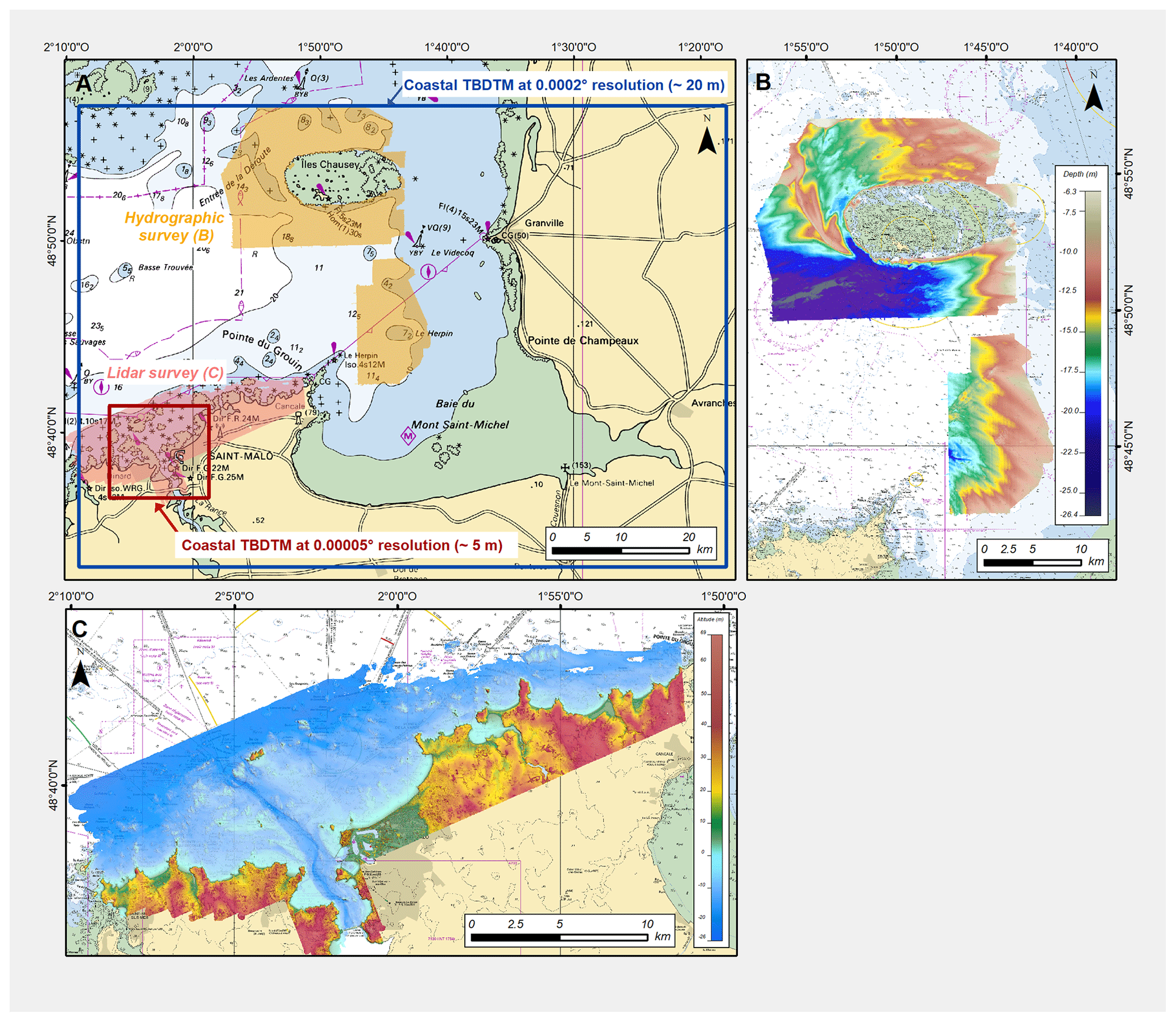
Figure 1 Nautical chart of Saint-Malo harbor and its surroundings (© Shom). (a) Locations of TBDTMs generated in the scope of Saint-Malo's PAPI project. (b) Bathymetric surveys carried out within the scope of PAPI Saint-Malo's project. (c) Bathymetric coverage of Brittany v.20190831 Litto3D^® maritime product of Saint-Malo harbor and its surroundings.

2 Topo-bathymetric dataset

The purpose of the following sections is to present the different data used for the generation of the TBDTMs (Fig. 1a), the most common problems experienced when combining data and the approach adopted by Shom for their resolution (Maspataud et al., 2015; Biscara et al., 2016).

2.1 Data sources

2.1.1 Bathymetric surveys

In the scope of the PAPI, the hydrographic vessels La Pérouse, Laplace and Borda were deployed between 2018 and 2019 in the Normand-Breton Gulf in order to update areas characterized precisely by a low-resolution bathymetric coverage. The surveys covered approximately 230 km² and ranged from −30 to +6 m water depth relative to the local chart datum (Fig. 1b). Table 1 details the schedule of the three bathymetric surveys carried out as part of the PAPI.

Table 1 Survey start and end dates for the three bathymetric surveys.

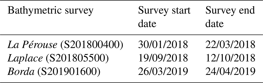
The hydrographic vessels are equipped with a Kongsberg Maritime EM710 multibeam echo sounder associated with the Seafloor Information System (SIS) software. Depending on the vessel, sound velocity profiles were measured using Sippican XBT probes or a Valeport SVP1000 sound velocity profiler to correct bathymetric data for local variations in sound speed. Real-time GPS positioning and roll, pitch and yaw information were collected with the Applanix POS MV inertial unit. Positioning data were post-processed in POSPac software using global navigation satellite system (GNSS) solutions. Horizontal positions were referenced to WGS84 or ITRF2014 geodetic systems at the time of the survey.

The bathymetric surveys were processed and qualified in accordance with the IHO S-44 standard that was in effect at the time the surveys were conducted (IHO, 2017a). The measured depths were corrected for various parameters, including system calibration factors, sensor offsets, attitude corrections, sound velocity and tide values, in order to reduce the soundings. Subset editing was carried out by a qualified hydrographer (FIG/IHO/ICA cat. B, IHO, 2017b) using CARIS HIPS and SIPS 9.1 to remove systematic errors and outliers. Processed and cleaned data were subjected to final validation by a senior qualified hydrographer (FIG/IHO/ICA cat. A, IHO, 2018). The total vertical uncertainty (TVU; IHO, 2017a) of these surveys at the 95 % confidence level is equal to 0.5 m. The total horizontal uncertainty (THU; IHO, 2017a) at the 95 % confidence level is between 0.55 and 3.1 m. With a minimum overlap between adjacent lines of more than 50 % of the half-swath, the three bathymetric surveys are compatible with orders 1a and 1b of the IHO S-44 standard.

2.1.2 Lidar data

Lidar surveys exploited in this study were carried out within the framework of the Litto3D^® program. This national program is based on a partnership between Shom and the French National Geographic Institute (IGN) (Louvart and Grateau, 2005). It aims to provide very-high-resolution coastal altimetric models of metropolitan and overseas French coasts (Pastol, 2011). Litto3D^® surveys are regularly implemented on Shom’s data portal (https://data.shom.fr, last access: 1 July 2024) under an open license. Coastal lidar mapping of the Normand-Breton Gulf was performed by Shom between 2016 and 2018, covering approximatively 700 km² and reaching up to 18 m water depth (Fig. 1c). Topo-bathymetric data were acquired from a Cessna Grand Caravan 208B aircraft equipped with an airborne lidar topo-bathymetric HawkEye III double hatch (Leica Geosystems). The data were acquired in relation to the ellipsoid and were referenced horizontally with respect to the RGF93 with a standard UTM 30N projection. The trajectory of the aircraft was based on the GNSS system and processed by Inertial Explorer. The trajectory data were post-processed using the stations of the RBF (Réseau de Base Français). The points were generated from the processed wave form with Lidar Survey Studio (LSS), and the point cloud was processed using PFMABE version 6.4.0.43 tools. The validation of the cleaned data was finally done by qualified hydrographers. Final point cloud data were reported to the IGN69 altimetry reference frame and to the Lambert 93 projection by the Circe Batch (V4-3, using RAF09 model) conversion tool.

2.1.3 Shom’s bathymetric database

Complementary bathymetric data used to generate the TBDTMs were extracted from Shom's bathymetric database (BDBS). A total of 52 bathymetric surveys (approximately 490 million soundings) conducted between 1829 and 2019 with different sounding methods (lead lines and single-beam and multibeam echo sounders) were available for the area of interest. Each survey extracted from the BDBS is associated with metadata, including the acquisition and processing methods, the IHO order survey, and the quality of the data. The spatial coverage of each survey is represented as a vector polygon layer (hereafter called a bounding polygon) that may adjoin, overlap or supersede older bathymetric surveys.

2.1.4 Other data

In addition to these bathymetric data, a bathymetric survey of the inner harbor delivered by the harbor authority of Saint-Malo was used in the present study. The bathymetric survey was carried out in June 2016 by the GEOXYZ society with a multibeam echo sounder. Soundings were vertically referenced to the chart datum of Saint-Malo. This bathymetric source was evaluated prior to integration into other datasets.

The RGE ALTI^® V2.0, produced by IGN, was exclusively used for the terrestrial domain. The data are available on IGN’s data portal (https://geoservices.ign.fr, last access: 1 July 2024) in the RGF93 geodetic system (Lambert 93 projection). The vertical datum of the data corresponds to the NGF-IGN69 legal system (IGN, 2018). The RGE ALTI^® v2.0 products used in the TBDTMs cover the departments of Côtes d'Armor, Ille et Vilaine and Manche at a resolution of 5 m. Data were clipped with a buffer extending 3 km inland. Water surface values were also eliminated using the raster layer of sources provided with the DTMs.

2.2 Production process

2.2.1 Convert data to a common horizontal and vertical datum

The key requirement for creating a seamless merged product is the homogeneity of the input datasets in terms of horizontal and vertical datum (Gesch and Wilson, 2001). The vertical transformation to the ellipsoid was performed with Circe 5.1 France (IGN) and Bathyelli V2.0 (Shom) for topographic and bathymetric data, respectively.

2.2.2 Data compilation

Selecting the most reliable source from multi-temporal and multi-sensor data is a fundamental challenge addressed in numerous works (Macnab and Jakobsson, 2000; Wong et al., 2007; Maspataud et al., 2015). This is particularly true for hydrographic offices, such as Shom, which have a considerable legacy of data. Bathymetric data have been collected using several sounding methods with specific characteristics of accuracy and precision.

Due to the scarcity and the difficulty of collecting bathymetric data, TBDTMs are produced from a process of data compilation. This process, also known as “deconfliction”, aims to ensure that the most relevant sources are selected to create the best possible representation. Until now, this tedious process was carried out manually in accordance with the S-44 standard and survey specifications (Maspataud et al., 2015; IHO, 2017a). To make it more efficient, Shom initiated the Téthys project in 2019 (Fig. 2). This in-house project aimed to constitute Shom’s bathymetric layer surface for which source data have been selected in order to generate the most accurate and up-to-date surface, satisfying the criteria related to the safety of navigation (Le Deunf et al., 2023). Overlap conflicts between surveys are resolved by a set of decision rules exploiting metadata (e.g., date, density, uncertainty and IHO order) which define whether a survey supersedes or completes older ones (Fig. 2b). In the case of a survey with a superseding status, the deconfliction process is executed by clipping the bounding polygon of the reference survey to fit all other older overlapping surveys. No clipping is done for surveys with a complete status (Fig. 2b). The resulting layer will be regularly updated on the basis of newly integrated surveys (Fig. 2c).

The generation of TBDTMs in the Normand-Breton Gulf benefited from the reliability of all metadata and bounding polygons in the area of interest, which constitutes the preliminary step prior to the construction of the Téthys. The deconfliction process was executed on all datasets used for the generation of the TBDTMs using routines based on modules (selection, filtering, masking, merging) available with GMT 5.1.1. (Wessel et al., 2013). The result of the deconfliction process corresponds to the most reliable soundings that can be used as input into the surface modeling.

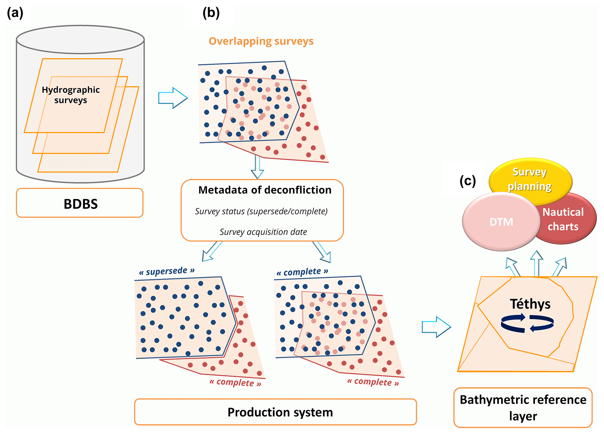
Figure 2 Workflow of Shom’s bathymetric reference layer (“Téthys”). (a) Shom’s bathymetric knowledge is composed of numerous overlapping surveys that are compiled in the BDBS. (b) In the case of overlapping surveys, a conflict resolution is applied based on the metadata of deconfliction. For bathymetric surveys which supersede older ones, the bounding polygon is used to clip the data. For bathymetric surveys which complete older ones, no action is performed. (c) Deconflicted data are compiled into one bathymetric reference layer for different applications. The reference layer will be updated each time a new survey is integrated into the BDBS.

2.2.3 Interpolation

Because multiple sources of data contribute to the construction of the DTM, some datasets have data point spacing larger than the required cell size. Spline functions are generally used for their efficiency when data densities vary. They produce a representative smooth and continuous surface. These may be more appropriate for large interpolation distances, which are frequently required for bathymetric data (Amante and Eakins, 2016, and references therein). Based on these observations, Shom used the SAGA (System for Automated Geoscientific Analyses; Conrad et al., 2015) software packages for the generation of the TBDTMs. The multilevel B-spline interpolation tool was used to perform surface modeling of the compiled data.

2.2.4 Altimetric conversion grids

Following NOAA’s previous works (Eakins and Taylor, 2010; Eakins et al., 2011), different datum altimetric grids were developed by Shom to convert the TBDTMs from the ellipsoid to other tidal datum (lowest astronomical tide and mean sea level). The creation of vertical reference surfaces at sea, linked to the ellipsoid, was initiated for metropolitan France with the BATHYELLI project (Pineau-Guillou and Dorst, 2013). The surface realizations used to convert TBDTMs correspond to the propagation of a vertical sea reference to all points in a tidal zone using a tidal model and a concordance equation.

2.2.5 Evaluation

The various checks carried out on the Téthys layer (reliability of attributes and bounding polygons, spatial coherence, etc.) provide a robust data compilation from which the bathymetric surface is modeled. The DTM is equally evaluated with qualitative and visual inspection (slope, cross-section and 3D views) and through additional layers (density, sources diagram). If possible, a cross-validation of the DTM with datasets that have not been incorporated into the generated product due to diffusion constraints is conducted. Despite the processing efforts and the deconfliction process, erroneous representation of the seafloor may remain. Preliminary versions of the TBDTMs highlighted two different types of artifacts:

• First of all, there is the overlapping of some bathymetric surveys with a complete status, leading to a noisy representation of the seafloor. In this case, the surface will not be suitable for modeling purposes despite the consistency amongst the surveys with respect to the S-44 standard. Therefore, the survey with the strongest TVU is clipped to generate a coherent surface.

• Secondly, an erroneous representation of depth can occur when three-dimensional data are far away, especially in unsurveyed marine areas (Eakins and Grothe, 2014; Danielson et al., 2016). In this configuration, the optimal fit of the B-spline multilevel model is not sufficiently constrained, the least-squares minimization is ill-posed, and the resulting model can generate unwanted oscillations. Locally, these artifacts are minimized by increasing the tension factor to smooth the surface.

As long as anomalies are detected, their cause must be determined and data must be reprocessed prior to a new interpolation. These different steps must be repeated iteratively until a satisfactory result is reached (Eakins and Taylor, 2010).

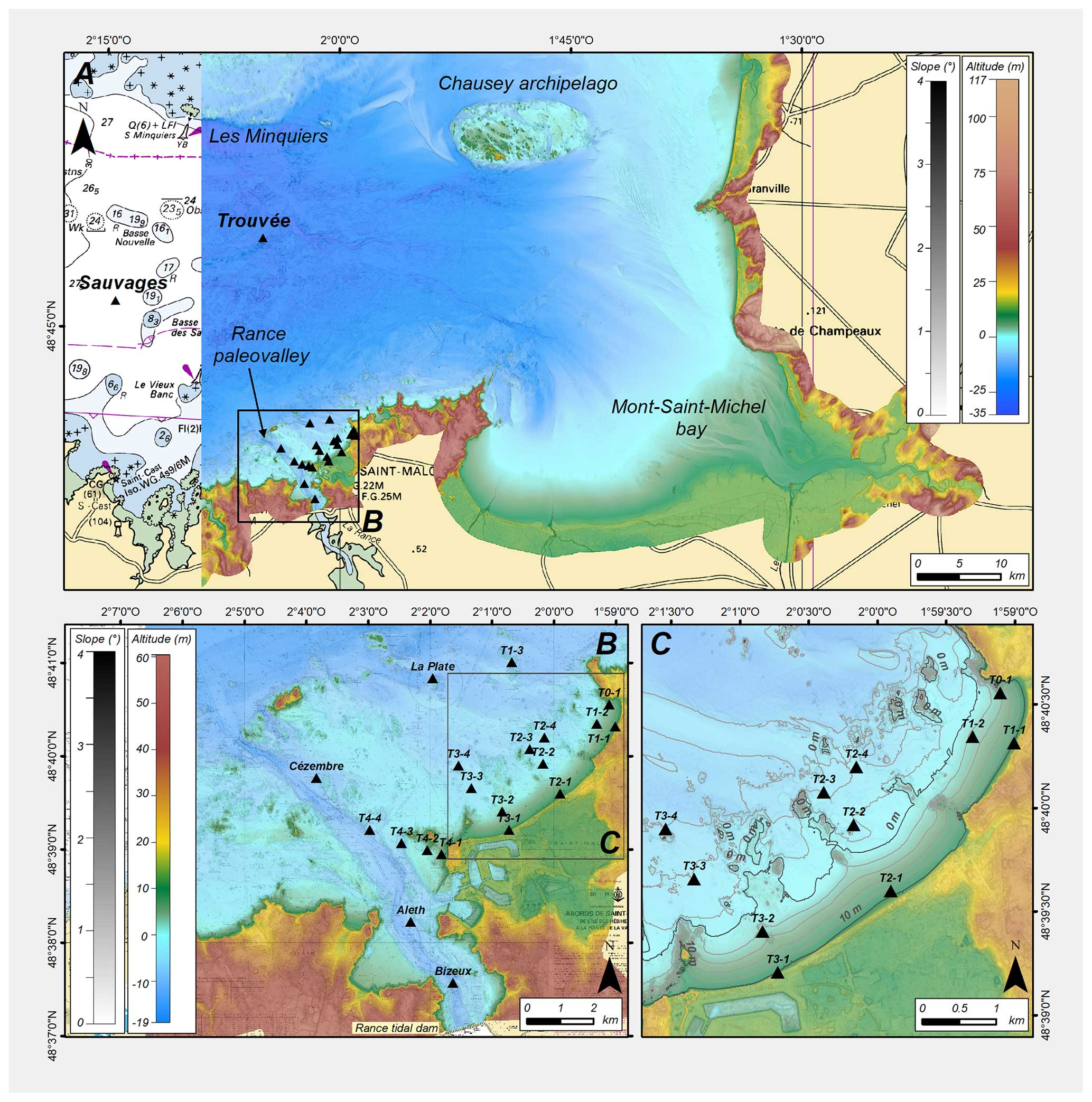
Figure 3 Nautical charts of the bay of Saint-Malo and its surroundings (© Shom). (a) Coastal TBDTM covering a part of the Normand-Breton Gulf at a resolution of 0.0002° (∼ 20 m and mooring positions); (b) coastal TBDTM of the harbor of Saint-Malo and its surroundings at a resolution of 0.00005° (∼ 5 m and mooring positions). (c) Zoom on the sensor transects.

2.3 Morphological description

Although the creation of TBDTMs is only a prerequisite for the flood forecasting model, it also enables us to describe the main morphological characteristics of the area under study. For the Saint-Malo harbor and its surrounding area, the TBDTM covers an area of 85 km² (Fig. 3b). At its center lies the mouth of the Rance, reaching a depth of around 10 m, 3 km downstream of the tidal power plant. The estuary extends further north, near the island of Cézembre, through an incision in the coastal shelf, along which the depth reaches 15 m. To the east of the estuary, there is an important accumulating bedform, the bench of Pourceaux, made of coarse sands (Bonnot-Courtois et al., 2002). The rest of the foreshore is characterized by smaller marine sedimentary deposits and submerged rocky structures, which provide partial protection from the prevailing northwesterly swells. In fact, it is considered to be an abrasion platform that evolves under very high hydrodynamic conditions and consequently has a poorly developed sedimentary prism (Daire et al., 2014). Apart from harbor infrastructures, the intertidal zone is characterized by sandy beaches in between rocky outcrops. The beaches are relatively small, with the largest, the beach of Sillon, stretching 3 km across a former marsh on which a large part of Saint-Malo is located. The beach is topped by a protective structure, the Paramé dike. Built in the 19th century, initially to protect industries and then the burgeoning seaside resort located in low-lying areas from erosion and flooding, the dike has suffered extensive storm damage over the years and has been repaired and remodeled many times over. On the TBDTM, the height of the dike now varies between 14.3 and 15.8 m above chart datum. However, in spite of the attempts to manage the coastal landscapes and the position of the coastline with dikes and embankments over the years, the shoreline has changed and will still evolve due to expected climatic and meteorological changes. Thus, acquiring these new topobathymetric data within the framework of the PAPI provides a snapshot of the coastline at a given moment. Sediment balances can be obtained by comparing them to older measurements, enabling the assessment of vulnerability to marine risks in this climatic context. Furthermore, through modeling and hydrodynamic data acquisition, a more accurate evaluation of flooding risks will be obtained, leading to more effective planning of coastal protection measures.

3 Oceanographic dataset

The oceanographic dataset includes water level, current and sea state observations from extensive in situ measurements conducted by Shom during winter 2018–2019 using different types of sensors. In the following, the field campaign and the data processing are described.

3.1 Oceanographic surveys

From October 2018 to April 2019, an extensive oceanographic campaign was conducted in the bay of Saint-Malo. The campaign includes 22 moorings, and each mooring containing one or two sensors, constituting a total of 37 sensors:

• 2 directional waveriders (Datawell, DWR-MkIII, hereafter referred to as Datawell)

• 2 tide pressure gauges (Sea-Bird Electronics, SBE26+, hereafter referred to as SBE)

• 4 acoustic wave and current profilers (Nortek, AWAC 600 kHz, hereafter referred to as AWAC)

• 4 single-point current meters (Nortek, Aquadopp single-point current meter, hereafter referred to as Aquadopp)

• 7 current profilers (Nortek, Aquadopp profiler 1 MHz, hereafter referred to as AquaPro)

• 18 wave pressure gauges (Ocean Sensor System Inc., 10 OSSI-010-003C and 8 OSSI-010-022, hereafter referred to as OSSI and OSSI-NEW, respectively).

The moorings were located so as to accurately describe hydrodynamic conditions from offshore to the coastline (Fig. 3). The Datawell buoys were deployed offshore at 25 m depth (Sauvages and Trouvée, Fig. 3a), providing information on the offshore wave fields. Other moorings were essentially deployed along four cross-shore transects (T1, T2, T3 and T4, Fig. 3b). Around the transects T1, T2 and T3, the beach profile is characterized by a gentle foreshore slope (2 %, Fig. 3c), increasing slightly (3 %) on the eastern part of the beach of Minihic (T0 sensor). Transect T4 is located in the vicinity of the Grand Bé islet and is characterized by high slope variations due to the presence of the Rance estuary (Fig. 3b). Two moorings, with OSSI and AquaPro, were deployed in the Rance estuary (Bizeux and Aleth, Fig. 3b). Table 2 summarizes the location of each mooring and sensor. For consistency with TBDTMs, the vertical datum used is the lowest astronomical tide (LAT).

Table 2 Details of moorings.

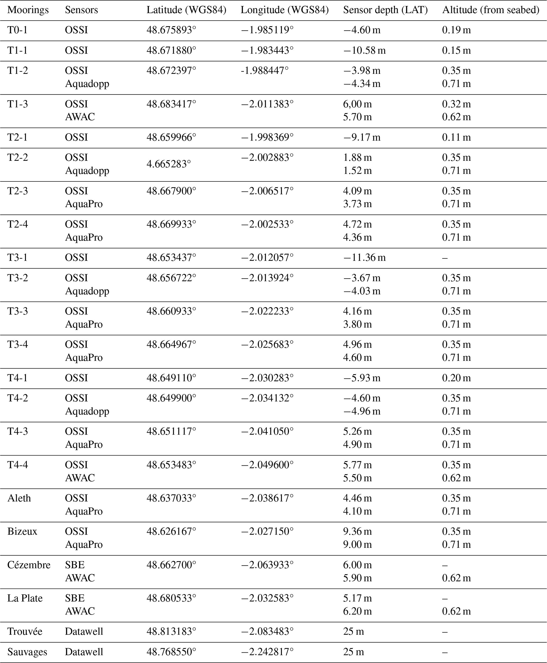
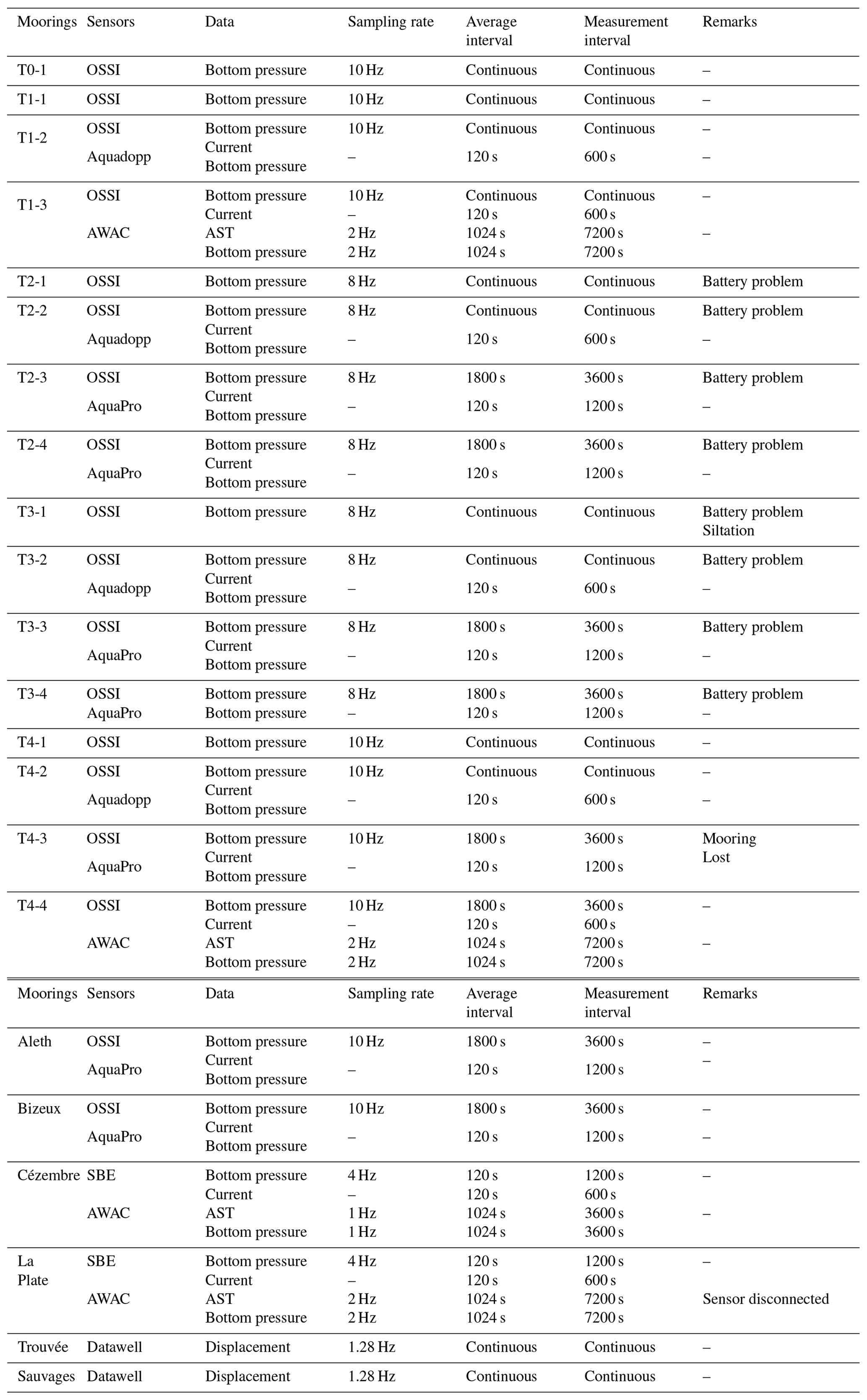
Sensors deployed during the campaign have been programmed to accurately record the oceanographic data, taking into account battery and data storage limitations. Sensor settings in terms of measurement data, sampling rate, average interval and measurement interval are summarized for each sensor in Table .

Table 3 Sensor acquisition protocol.

3.1.1 Sensor acquisition

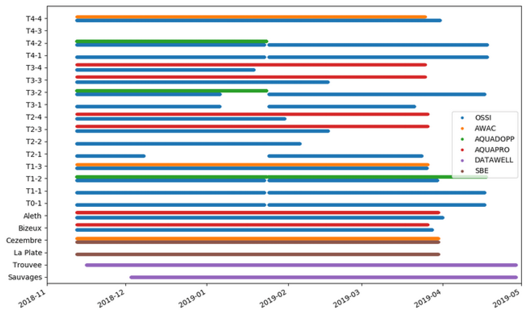
Figure 4 presents a summary report of sensor acquisition. All moorings, except buoys, started on 12 November 2018. The last acquisitions were on 30 March and 20 April for foreshore or offshore moorings, respectively. The acquisitions of Datawell buoys began on 15 November 2018 for the Trouvée mooring and on 2 December 2018 for the Sauvages mooring, continuing until 29 April 2019 for both buoys. Figure 4 shows interruptions in data acquisition for OSSI-NEW in transects T2 and T3. These interruptions were caused by less efficient batteries than anticipated on the OSSI-NEW (as mentioned in Table ). For moorings on the foreshore, a brief interruption in the data acquisition appeared from 22 January to 24 January. This interruption was planned for a battery change. The La Plate AWAC sensor did not acquire any data during the campaign (the sensor power cable was disconnected). The mooring T4-3 with all the sensors unfortunately remains unrecovered, probably due to a malicious act. Despite these incidents, the density and complementarity of the instruments used during the campaign give a homogeneous description of the hydrodynamics in the bay of Saint-Malo. The data collection covers a winter period of more than 4 months.

Figure 4 Mooring acquisition report.

3.2 Data processing

The workflow for generating the oceanographic dataset consists of three steps:

• Pre-process binary data using the manufacturers’ software.

• Process the data using the Python toolbox SCOT developed for this study.

• Write data and metadata to NetCDF format.

3.2.1 Water levels

The water levels are mainly monitored by pressure sensors, including a tide pressure gauge (SBE) and a wave pressure gauge (OSSI), using different sampling frequencies and acquisition plans (Table ). Current meters (Aquadopp, AquaPro or AWAC) are also equipped with pressure sensors.

The tide pressure gauges also record the 2 min averaged bottom pressure every 20 min. The raw data were converted to water level h assuming hydrostatic equilibrium (Eq. 1):

$$\begin{array}{}\text{(1)}& h={\displaystyle \frac{P_{\mathrm{m}}-P_{\mathrm{atm}}}{\mathit{\rho }g}}+{\mathit{\delta }}_{\mathrm{m}},\end{array}$$

where P_m stands for the bottom pressure measurement in Pa, P_atm is the atmospheric pressure extracted from ERA5 atmospheric reanalysis (in Pa), ρ=1026 kg m⁻³ is the averaged water density measured in the bay of Saint-Malo, δ_m is the sensor’s distance from the bed (in m), and g=9.81 m s⁻² is the gravitational acceleration. Note that the data from ERA5 reanalysis were preferred over the measurements at Dinard airport meteorological station due to acquisition problems.

The wave pressure gauges and current meter with pressure sensors record bottom pressure at higher frequencies (see Table ). In the case of continuous measurements, the data recorded in ASCII format were aggregated in consecutive bursts of prescribed length (20 min here). The raw pressure data of each sensor are calibrated using the pressure slope and offset of the sensor. For foreshore sensors, the calibration is performed by comparing the burst-averaged pressure measured whenever the sensor is out of water to the atmospheric pressure (e.g., see Appendix C). For offshore sensors, the pressure sensor was calibrated before or at the end of the recording when the instrument was taken out of the water. Then, the corrected pressure was converted into water level assuming hydrostatic equilibrium (Eq. 1). Finally, to reconstruct water level for the long waves, such as tide, the water level was smoothed with a moving average of 10 min to filter out deformations of the water surface related to short waves.

In order to compare water levels recorded with different instruments, the measurements were relocated in terms of height with respect to the tide gauge of Saint-Malo harbor (e.g., see Appendix C). The correction factors (slope and offset) from the Saint-Malo tide gauge are provided in the dataset for each sensor. The accuracy of water levels is on the order of ±5 cm. For consistency with TBDTMs, the vertical datum used is the lowest astronomical tide (LAT).

Finally, acoustic surface tracking (AST) with vertical beams performed by AWAC current meters allows the sampling of the surface elevation.

3.2.2 Currents

The currents are monitored by the acoustic Doppler current using single-point current meters (Aquadopp) and current profilers (AquaPro and AWAC). These sensors record the speeds on the axis of their three beams. The raw binary data file was directly processed by the Python toolbox SCOT developed for this study. First, the velocity data are reprojected to a terrestrial landmark on the northeast-vertical axes. Prior to their deployment, the magnetic compasses of these current meters were previously calibrated on a dedicated Shom platform. The calibration procedure and the uncertainty of current data are described in Le Menn and Morvan (2020). Finally the current data and metadata of each sensor are written in NetCDF format.

3.2.3 Sea states

The sea states are monitored by three different types of sensors: a directional wave buoy, a wave pressure gauge, and an acoustic wave and current profiler.

The directional wave buoys recorded wave displacements in the three directions of the ENU frame using measurements from accelerometers, inclinometers and a compass. First, a quality-controlling procedure is performed on each for 30 min bursts, such that a burst is discarded if at least one of the three displacements is outside the range ±4σ, where σ is the standard deviation of the time series. Then, the cross-spectra of the displacements were computed by means of a fast Fourier transform (FFT) on 10 Hanning-windowed segments with a 50 % overlap, which allows a good compromise between statistical stability (20 degrees of freedom) and frequency resolution (5.5 mHz). The power spectral density of vertical displacements is used for estimating the main bulk parameters (see Appendix B), while the five other independent co- and quad-spectra are used to compute the main directional parameters and to estimate the directional distribution using the iterative maximum likelihood method (IMLM) with an angular resolution of 5° (e.g., see Oltman-Shay and Guza, 1984) so as to compute an estimate of the directional spectra.

For the wave pressure gauges, the free surface elevation signal associated with waves was first reconstructed from bottom pressure measurements so as to account for the non-hydrostatic effects. A recent review of Mouragues et al. (2019) provides different methods depending on the assumptions made regarding the wave field’s dispersive properties. In addition to the hydrostatic reconstruction, the linear method and the non-linear weakly dispersive method (see Appendix A) were thus applied to each burst after detrending so as to suppress tidal motion. The wave spectra were computed as described above (resulting in 20 degrees of freedom and a frequency resolution of 5.5 mHz) to finally compute spectral estimates of the bulk parameters in addition to the wave-by-wave analysis (see Appendix B).

The AWAC records surface elevation from acoustic surface tracking (AST) and the two components of the horizontal current in the east–north–up frame (ENU) within a sub-surface wave cell at high frequency. First, a quality-controlling procedure is performed on each burst based on the QC flag associated with AST measurements, such that a burst is discarded when the first quartile of the QC flag distribution is below 100, which corresponds to the ceil below which the measurement is considered to be dubious (Nortek support team, personal communication, 2023). Then, the cross-spectra of the measurement triplet were computed as described above (resulting in 20 degrees of freedom and a frequency resolution of 7.8 mHz), and the same processing as for the directional wave buoy measurements was performed (e.g., see Krogstad et al., 1988, for the estimate of the directional distribution from acoustic Doppler current profiler (ADCP) measurements using the IMLM).

4 Applications of these datasets

Section 4 aims to provide some insights into the benefits of such datasets. The first one is that they allow us to understand, identify and quantify key processes of coastal flooding. A second benefit is that they are crucial in the development, as well as in the calibration and validation, of a high-resolution coupled surge–wave model, which is expected as part of the preliminary PAPI study.

4.1 Overview of oceanographic processes

Figure 5a, b and c show an overview of the temporal evolution of the metocean conditions during the studied period. First, several low-pressure systems affected Saint-Malo. These storm events produced skew surges (that is, the difference between the maximum observed sea level and the maximum predicted tide regardless of their timing during the tidal cycle) from 22 to 61 cm and offshore significant wave heights H_m0 from 2.29 to 4.28 m. These storms occur principally during neap tides. No coastal flooding was observed during this experiment. The storm events associated with two major spring tides are reported in Table 4 with the corresponding metocean conditions.

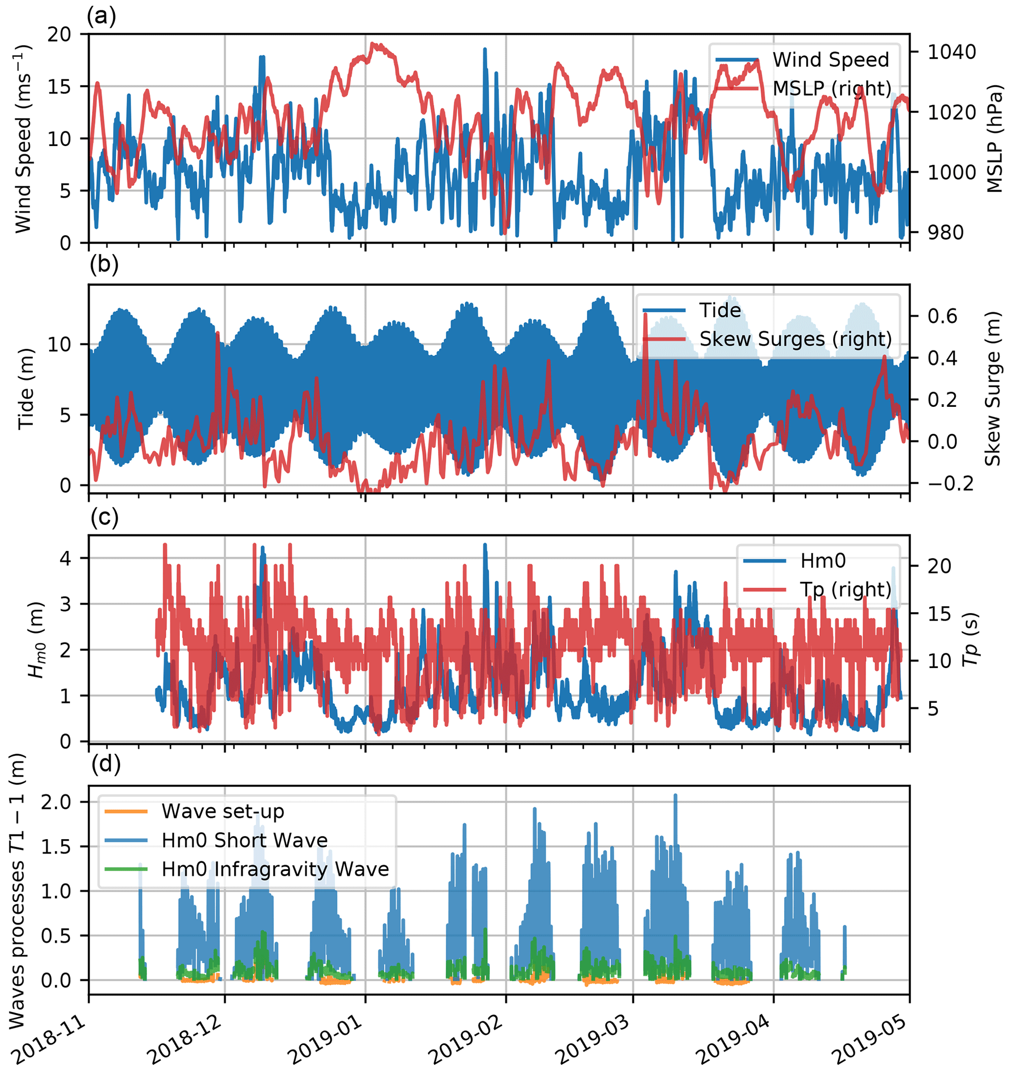
Figure 5 (a) Wind speed and mean sea level pressure (MSLP) from ERA5 reanalysis in Saint-Malo. (b) Tide prediction and skew surge at Saint-Malo harbor tide gauge. (c) Significant wave height H_m0 and peak period at Trouvée buoy. (d) Short and infragravity significant waves height and wave set-up at T1-1.

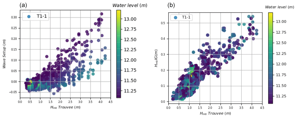
Figure 6 Wave set-up (a) and infragravity significant wave height (b) at T1-1 mooring according to offshore significant wave height and water level (color).

Table 4 Inventory of metocean conditions (wave conditions at Trouvée) and wave processes at T1-1 during storm events and major spring tide events of field experiment.

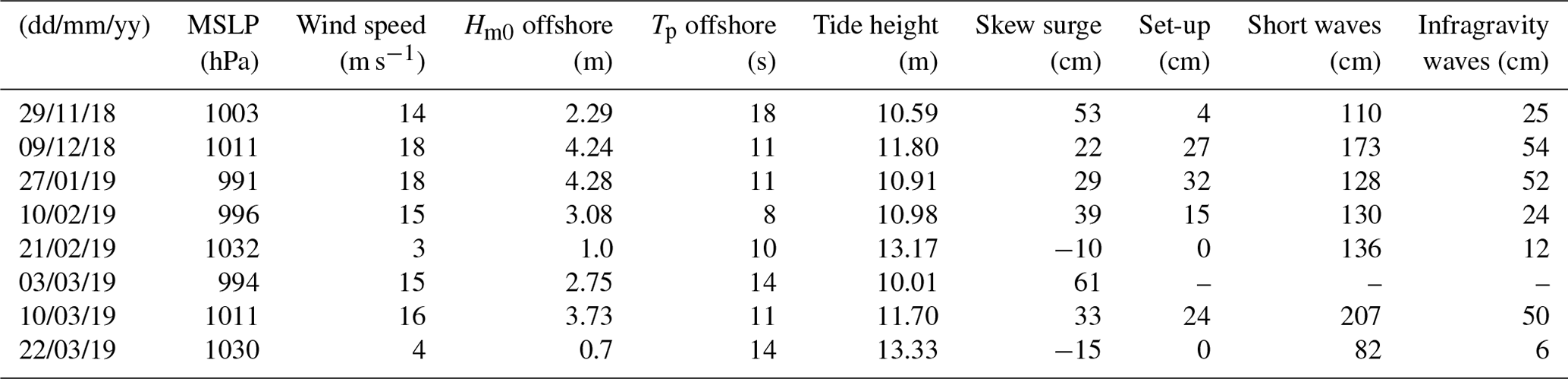
The wave transformation induces further processes affecting water level elevation, such as wave set-up and infragravity waves (e.g., see Dodet et al., 2018). Figure 5d shows the wave set-up estimated from the difference in water level between sensor T1-1 and T1-2 and the infragravity significant wave height (between 0.004 and 0.04 Hz) at T1-1. The maximum wave set-up was measured during the 9 December 2018, 27 January 2019 and 10 March 2019 storms (Table 4), with wave set-up measurements of around 27, 32 and 24 cm, respectively. The maximum infragravity significant wave heights also occurred during these storms, with heights greater than 50 cm. Table 4 indicates the wave set-up and the short and infragravity significant wave heights at T1-1 for each storm concomitantly with the spring tide event. Figure 6 shows the wave set-up estimates and the infragravity significant wave height versus the offshore significant wave height associated with the corresponding water levels. The wave set-up and the infragravity significant wave height increase with the offshore significant wave height as expected (the correlation coefficients are equal to 0.75 and 0.77, respectively). The wave set-up appears to be closely related to the water level, with higher wave set-up at rising and falling tide, whereas, at high tide (sea levels >12 m), the wave set-up is of the order of 10 cm for offshore waves of 4 m. On the contrary, no major correlation is found between the water level and the infragravity significant wave height.

The oceanographic dataset provides, for the first time, observations of processes that can lead to marine flooding in the bay of Saint-Malo. Even though the measurement period did not include any flood events, the wave set-up (which was found to be negligible at high tide) is unlikely to be the main cause of flooding. Flooding typically occurs at high tide, when tidal coefficients are high. On the contrary, short and infragravity waves that remain high at the foot of the dike seem to have a major impact and can be responsible for over-topping, which is often observed but unfortunately not measured.

4.2 Implementation of numerical configuration for a local coastal flood warning system

One of the objectives of the PAPI for the Saint-Malo Agglomeration is to evaluate the feasibility and interest of setting up a local marine flood forecasting system in relation to the national system. In addition to improving the knowledge of the processes responsible for the flooding in this area, the data presented in this paper are the essential prelude to the implementation, calibration and/or validation of the hydrodynamic models that underlie this forecasting service. We present here an overview of this system, which is currently the subject of ongoing efforts.

The tide, surge and wave modeling of the French national system is based on the barotropic circulation model HYCOM (Bleck, 2002) and on the wave model WAVEWATCH III^® (hereinafter WW3, The WAVEWATCH III® Development Group, 2016), coupled with the Oasis coupler (Valcke et al., 2015).

The French Atlantic configuration (hereinafter called HR) that is operationally run in the Météo-France storm surge forecast system has a resolution of 600 m at nearshore scale, which is insufficient for forecasting flooding at the scale of a city like Saint-Malo. In the context of the PAPI, nested grids for both wave and surge models were generated with resolutions of up to 30 m at the coastline (the same methodology for Pertuis Charentais is described in Michaud et al., 2015; Pasquet et al., 2021). The Oasis coupler was used to provide boundary conditions of the HYCOM nested configurations, as well as of the coupling between the 30 m resolution onshore WW3 and HYCOM configurations. The overall system relies on curvilinear grids for HYCOM and unstructured grids for WW3. The bathymetry part of the coastal 20 m resolution TBDTM referenced to mean sea level, presented in this paper, was interpolated on the curvilinear HYCOM grids (whose onshore limits are the coastline) and the WW3 mesh. This unstructured mesh was generated using the PolyMesh 2D Mesh Generator, developed at BGS IT&E. The mesh resolution varies throughout the domain, from 50 m offshore to 30 m onshore, due to the mesh criteria chosen in relation to depth gradient and Courant–Friedrichs–Lewy (CFL) to optimize node distribution. The coupling follows the vortex–force approach (Ardhuin et al., 2008; Bennis et al., 2011; Michaud et al., 2012), and the exchanges of all the variables (the current, water level and mask variables from HYCOM and sea state variables from WW3) are done every 10 min. This modeling system, called THR, allows us to represent some nearshore processes such as wave breaking and wave set-up thanks to the high resolution and the coupling between models.

It is worth noting that the high resolution of the TBDTM (5 m) and the spatial density of the dataset would allow a set-up of the model with refined computational grids. The choice of the resolution at the coast is a good compromise considering the (phase-averaged) modeling approach adopted here, along with the practical aspects regarding model implementation and the computational cost. First, a finer resolution would have been too costly for operational purposes. Second, increasing the resolution at the coast with nested grids would require an additional intermediate grid in HYCOM. Finally a phase-resolving modeling approach, allowing an explicit representation of the free surface, and a better representation of wave transformations on a coastal scale would be more appropriate at a higher resolution. Such models are currently too expensive for operational use at a national level, although benefiting from active developments in the numerics to reduce their computational cost (Couderc et al., 2017; Marsaleix et al., 2019; Duran et al., 2020; Richard, 2021).

Models were calibrated and validated using the series of measurements in the bay of Saint-Malo(Seyfried et al., 2021). The breaking index was set to 0.5 in the WW3 configuration. The bottom stress parameterization in HYCOM uses a semi-quadratic formulation with bottom drag coefficient maps obtained using stochastic optimization based on – and assessed with – water level observations or predictions.

This modeling system allows the observation of the wave field transformation at the entrance to the bay of Saint-Malo, with an eastern part of the bay being highly exposed and a western part being less exposed as it is protected by the island of Cézembre (see Fig. 7a for the 9 December 2018 storm at high tide). The significant wave height H_m0 decreases from the entrance to the bay to the foot of the dikes, mainly due to wave breaking in the bay of Saint-Malo and interactions with the numerous obstacles (islands, shoals, groynes). The spatial variability of H_m0 is well represented for this event, as shown by the comparison with observation points. The simulated surge (atmospherical and wave set-up) during the 9 December storm at high tide shows a gradient from the open sea to the coast, marked as particularly close to the shore defenses, after the breaking zone (Fig. 7b), linked to the generation of a wave set-up. In the estuary and outer harbor, the effect of the wave set-up is negligible. Comparison with the observation points shows an underestimation of the surge offshore but a good representation of the surge increase at the foot of the structures (moorings T1-1 and T4-1). The model depicts lower surges at certain points in the bay, particularly in some shoals, which are areas of shallow water that induce a shoaling and a set-down. This is also observed at moorings T3-3 and T3-4, which are positioned on shoals, where there are lower surges than at other moorings. However, the resolution of 30 m and uncertainties in data that are of the order of 5 to 10 cm make point-to-point model interpretation and validation difficult.

While being an important process at low tide, simulations and observations reveal that wave set-up is negligible at high tide and thus seems not to be a dominant process responsible for coastal flooding (Seyfried et al., 2021). In fact, the observational period did not include any coastal flooding due to major storms, but statistical analysis (Seyfried et al., 2021) and the high tidal range at Saint-Malo mean that coastal flooding occurs during large tides with high tidal coefficients. Certain processes, such as infra-gravitational waves or wave over-topping processes, have shown a non-negligible impact on flooding thanks to measurements or observations made during the sea campaign remaining unrepresented in the model. The modeling system developed in this study is thus insufficient and would need to be complemented at the nearshore scale by a phase-resolved model to represent the infra-gravity waves, as well as over-topping. However, this modeling system is the necessary link between the models operated at a national scale and these high-resolution phase-resolved models.

Additional measurements would therefore be needed to calibrate and validate this phase-resolved model, particularly with cameras, pressure gauges or lidar stations on the dike, for the wave over-topping measurement. In addition, another strategy based on permanent networks with low-sampling, low-power systems with continuous data transmission could also be complemented by model assimilation and machine learning algorithms to adaptively improve forecasting accuracy over time and to add robustness and resilience to the system. This strategy would include collaborative aspects, involving stakeholders and local authorities, ensuring its success.

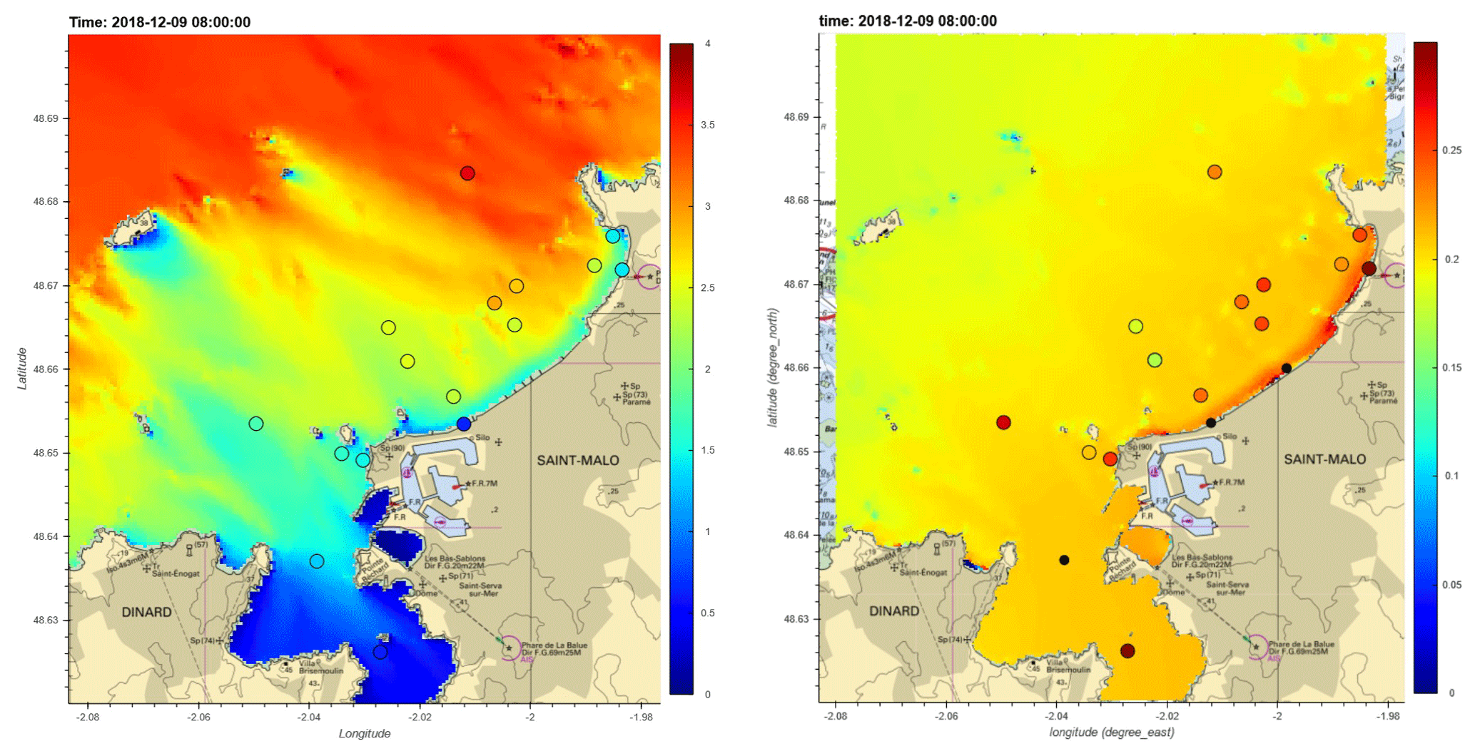
Figure 7 Map of significant wave height (left) and surge (atmospherical and wave set-up) (right) in meters at high tide, as simulated by the THR system, during the 9 December 2018 storm. The colors of the dots represent the measured value at the various moorings during this event.

5 Data availability

The TBDTMs (Shom, 2020a, b) and oceanographic datasets (Shom, 2021) are freely available at the following:

• https://doi.org/10.17183/MNT_COTIER_GNB_PAPI_SM_20m_WGS84 (Shom, 2020a)

• https://doi.org/10.17183/MNT_COTIER_PORT_SM_PAPI_SM_5m_WGS84 (Shom, 2020b)

• https://doi.org/10.17183/CAMPAGNE_OCEANO_STMALO (Shom, 2021).

The TBDTM is released through pre-packed files, outlined as follows:

• files containing bathymetric surfaces, vertically referenced to different vertical datum (mean sea level or lowest astronomical tide) and converted to four grid formats, including NetCDF format (.grd by GMT), bathymetric attributed grid (.bag), ESRI ASCII raster format (.asc) and ASCII text format (.glz);

• a metadata file that contains data sources, geographical extent, legal constraints and a brief summary of the building process, meeting the requirements of the INSPIRE Directive;

• the citation and an associated digital object identifier (unique identifier used to cite scientific articles and datasets) to easily identify the future multiple uses of the DTM;

• the rights and contents report describing the main features of the product and its limitations.

The oceanographic dataset is available through four levels of processing, outlined as follows:

• L0 is the direct output of sensors in binary or ASCII format.

• L1 is the processed outputs of sensors in ASCII format using the manufacturers’ software.

• L2 is processed data and metadata in NetCDF format.

• L3 is post-processed integrated or peak-to-peak wave parameters in NetCDF format.

6 Conclusions

The acquisition of new topo-bathymetric data in the bay of Saint-Malo allowed the creation of a topo-bathymetric dataset. This dataset contains two TBDTMs with resolutions of 20 and 5 m. An extensive oceanographic campaign was also carried out to create a dataset that provides a set of oceanographic parameters (water levels, currents and sea states) in the bay of Saint-Malo for different atmospheric, tidal and sea state conditions.

During the oceanographic campaign, three moderate storms occurred in the bay of Saint-Malo, the observation of which allows us to analyze the different oceanographic processes involved in coastal flooding specific to this area. The dataset provides, for the first time, a measurement of the wave transformation in the bay of Saint-Malo and a quantification of the wave processes at the foot of the protection structures. In this macro-tidal area, the variation in the water level plays a major role in wave processes. At high spring tide, the short and the infragravity waves spread up to the protection structures. The wave set-up is not established, but over-topping by sea pack may occur (not measured).

Topo-bathymetric and oceanographic datasets are useful to build, validate and calibrate wave and hydrodynamic models. In the context of the PAPI, a local coastal flood system has been developed to reproduce the surge and waves at a high resolution in the bay of Saint-Malo. Comparison and calibration with measurements have been conducted and show that this high-resolution model clearly improves the representation of wave dissipation and surge in the bay and, therefore, the national marine flood forecasting system. It provides the right information, refined in resolution and precision, to set up a first level of impact indicators at a local scale. However, some observed processes, such as infra-gravitational waves or wave over-topping, remain unrepresented in the model. The coupled system is thus the essential link in the chain to complete the coastal forecasting capability with a phase-resolved model that would enable the modeling of all the processes responsible for a potential flooding event.

Finally, although this type of dataset is costly to build and is limited in space and time, it enables the characterization of processes at short temporal scales, complementing the satellite altimetry monitoring of coastal variables, which face strong limitations in coastal areas. Establishing permanent national networks, with continuous data transmission, complemented by model assimilation and machine learning algorithms to adaptively enhance forecasting accuracy over time and to add robustness and resilience to the system, seems to be a promising way forward.

Appendix A: Surface elevation reconstruction method based on bottom pressure

Three different reconstruction methods were used.

A1 Hydrostatic reconstruction

The hydrostatic reconstruction based on the hydrostatic equilibrium is done as follows:

$$\begin{array}{}\text{(A1)}& {\mathit{\zeta }}_{\mathrm{h}}=h-h_{\mathrm{0}}+{\mathit{\delta }}_{\mathrm{m}},\end{array}$$

with ζ_h being the hydrostatic free surface elevation (in m), h₀ being the mean water depth (in m) and δ_m being the sensor’s distance from the bed (in m).

A2 Linear reconstruction

The linear reconstruction based on a transfer function derived from the linear wave theory (TFM) is the most commonly used method (e.g., see Bishop and Donelan, 1987):

$$\begin{array}{}\text{(A2)}& F\mathit{\left\{}{\mathit{\zeta }}_{\mathrm{linear}}\mathit{\right\}}=K_{\mathrm{p}}\left(\mathit{\omega }\right)F\mathit{\left\{}{\mathit{\zeta }}_{\mathrm{h}}\mathit{\right\}},\end{array}$$

where F{⋅} corresponds to the Fourier transform, and K_p(ω) is the transfer function.

$$\begin{array}{}\text{(A3)}& K_{\mathrm{p}}\left(\mathit{\omega }\right)={\displaystyle \frac{\cosh \left(k\right(\mathit{\omega }\left)h_{\mathrm{0}}\right)}{\cosh \left(k\right(\mathit{\omega }\left){\mathit{\delta }}_{\mathrm{m}}\right)}}\end{array}$$

Solving this equation requires the use of the dispersion relation issued from linear wave theory:

$$\begin{array}{}\text{(A4)}& {\mathit{\omega }}^{\mathrm{2}}=gk\tanh \left(k{h}_{\mathrm{0}}\right).\end{array}$$

This method requires an upper cut-off frequency so as to remove high-frequency noise that is amplified by the transfer function and to prevent the over-amplification of high-frequency energy levels due to non-linear interactions in intermediate and shallow waters (e.g., see Bonneton and Lannes, 2017; Bonneton et al., 2018; Mouragues et al., 2019; Martins et al., 2020). For frequencies exceeding the limit frequency, the correction factor can be replaced by different values (K_p=1, sharp cut-off – the linear spectrum is replaced by hydrostatic spectrum), linear correction factors, steady correction factors and the JONSWAP spectrum (see Mouragues et al., 2019, for a description of these methods). The optimizations of the cut-off frequency and correction factor are a source of improvement in the representation of the wave shape (Mouragues et al., 2019; Martins et al., 2020). In this study, in order to simplify the treatment and make it homogeneous, a sharp cut-off frequency of 0.25 Hz was chosen for the whole dataset.

A3 Non-linear weakly dispersive reconstruction

The non-linear weakly dispersive (swnl) reconstruction (Eq. A5) was introduced by Bonneton et al. (2018). This method consists of reconstructing surface wave elevation from non-linear wave theory for weakly dispersive waves.

$$\begin{array}{}\text{(A5)}& {\mathit{\zeta }}_{\mathrm{swnl}}={\mathit{\zeta }}_{\mathrm{swl}}-{\displaystyle \frac{\mathrm{1}}{g}}\left[{\partial }_t\left({\mathit{\zeta }}_{\mathrm{swl}}{\partial }_t{\mathit{\zeta }}_{\mathrm{swl}}\right)-{\left({\displaystyle \frac{{\mathit{\delta }}_{\mathrm{m}}}{h_{\mathrm{0}}}}\right)}^{\mathrm{2}}{\left({\partial }_t{\mathit{\zeta }}_{\mathrm{swl}}\right)}^{\mathrm{2}}\right]\end{array}$$

In the above, ζ_swl is the free surface elevation from the linear weakly dispersive reconstruction:

$$\begin{array}{}\text{(A6)}& {\mathit{\zeta }}_{\mathrm{swl}}={\mathit{\zeta }}_{\mathrm{h}}-{\displaystyle \frac{h_{\mathrm{0}}}{\mathrm{2}g}}\left[\mathrm{1}-{\left({\displaystyle \frac{{\mathit{\delta }}_{\mathrm{m}}}{h_{\mathrm{0}}}}\right)}^{\mathrm{2}}\right]{\partial }_t^{\mathrm{2}}{\mathit{\zeta }}_{\mathrm{h}}.\end{array}$$

As opposed to the TFM, the resolution of Eq. (A5) does not require the use of a dispersion relationship. However, this transformation requires the intrusion of a cut-off frequency to filter the measurement noise (Mouragues et al., 2019). In this study, in order to simplify the treatment and make it homogeneous, a cut-off frequency of 0.5 Hz was chosen for the whole dataset. This method allows a better reconstruction of the height of the highest waves near the breaking point (Mouragues et al., 2019); however, its application is limited to a weakly dispersive wave regime.

A comparison of free surface elevation with the different methods and with the AST acquisition is shown in Fig. A1 for high and low tide. The parameter H_m0 is also given for the different methods and sensors.

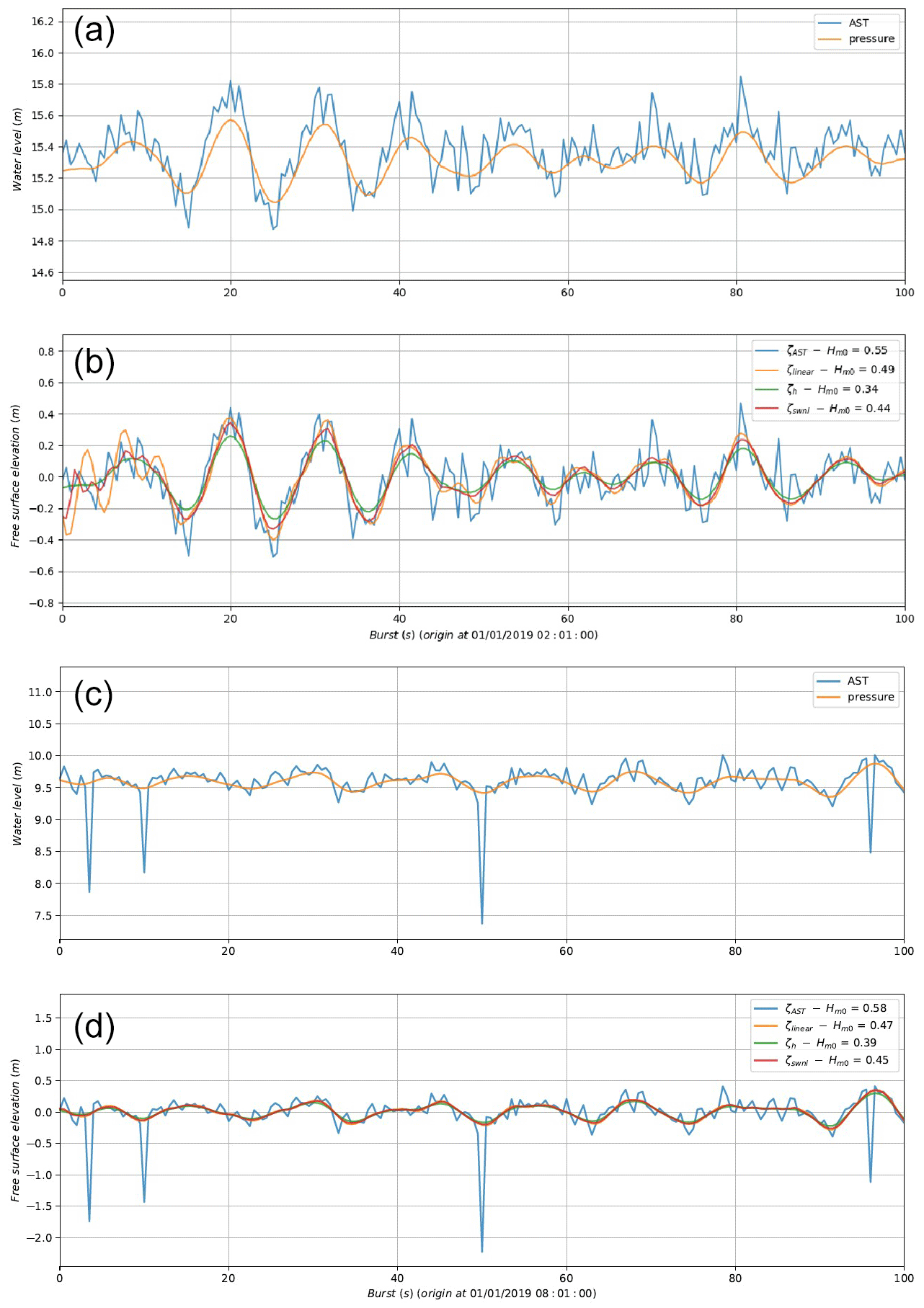
Figure A1 Comparison of free surface elevation with the different methods and with the AST acquisition for high (a, b) and low (c, d) tide. The value of H_m0 is also given for the different methods.

Appendix B: Bulk parameters: spectral estimates and wave-by-wave analysis

The spectral significant wave height(H_m0), mean periods ($T_{m_{\mathrm{0}n}}$) and continuous peak period (T_pc) were computed using the nth moment of the wave spectra (with E corresponding to the power spectral density of the elevation signal), which reads as follows:

$$\begin{array}{}\text{(B1)}& m_n=\underset{f_{\min }}{\overset{f_{\max }}{\int }}{f}^{n}E\left(f\right)\mathrm{d}f,\end{array}$$

such that

$$\begin{array}{}\text{(B2)}& {\displaystyle }{H}_{\mathrm{m}\mathrm{0}}=\mathrm{4}\sqrt{m_{\mathrm{0}}}\text{(B3)}& {\displaystyle }{T}_{m_{\mathrm{0}n}}={\left({\displaystyle \frac{m_{\mathrm{0}}}{m_n}}\right)}^{\mathrm{1}/n}\text{(B4)}& {\displaystyle }{T}_{\mathrm{pc}}={\displaystyle \frac{m_{-\mathrm{2}}{m}_{\mathrm{1}}}{m_{\mathrm{0}}^{\mathrm{2}}}}.\end{array}$$

On the other hand, the discrete peak period was computed from the spectral maximum at the peak frequency f_peak as $T_{\mathrm{peak}}=\mathrm{1}/f_{\mathrm{peak}}$. As an initial approach, the lower bound f_min used for computing the moments of the wave spectra was set to 0.04 Hz; note, however, that a convenient separation between the infragravity band and the gravity band might be defined as half the offshore peak frequency (e.g., see Hamm and Peronnard, 1997; Bertin et al., 2020). The upper bound f_max was consistently set to f_c=0.2 Hz for wave pressure gauges and 0.4 Hz for the wave buoys and the AWAC.

Considering a well-sampled and detrended time series of free surface elevation, an individual wave is defined, by convention, as the elevation profile between two consecutive instants of downward zero crossing. The height (H) of an individual wave is then defined as the difference between the maximum (the crest) and minimum (the trough) values of elevation, while the period (T) is the time separating the final instant from the initial instant. In practice, a peak is defined as any sample whose two direct neighbors have a smaller amplitude, with a minimum distance between two peaks roughly corresponding to a minimum period set to 4 s and a minimum amplitude ($\simeq H/\mathrm{2}$) set to 0.1 m. For flat peaks (i.e., more than one sample of equal amplitude in width), the index of the middle sample is returned, rounded down in case the number of samples is even. Given the minimum period and the length of a burst, one can estimate the upper limit of observable waves per burst. If the number of waves actually detected does not exceed 10 %, the burst is rejected. For N waves detected in the time series, the mean wave height ($\stackrel{\mathrm{‾}}{H}$) and mean wave period ($\stackrel{\mathrm{‾}}{T}$) are given by

$$\begin{array}{}\text{(B5)}& {\displaystyle }\stackrel{\mathrm{‾}}{H}={\displaystyle \frac{\mathrm{1}}{N}}\sum _{i=\mathrm{1}}^N{H}_i,\text{(B6)}& {\displaystyle }\stackrel{\mathrm{‾}}{T}={\displaystyle \frac{\mathrm{1}}{N}}\sum _{i=\mathrm{1}}^N{T}_i.\end{array}$$

The significant wave height is computed as the mean value of the top one-third of the largest waves in the distribution:

$$\begin{array}{}\text{(B7)}& H_{\mathrm{1}/\mathrm{3}}={\displaystyle \frac{\mathrm{1}}{N/\mathrm{3}}}\sum _{j=\mathrm{2}N/\mathrm{3}}^N{H}_j,\end{array}$$

where j is the index of the waves sorted in ascending order. The maximal wave height (H_max) is also computed from the wave-by-wave analysis:

$$\begin{array}{}\text{(B8)}& H_{\max }=\underset{i\in \left[\right[\mathrm{1},N\left]\right]}{max}\left(H_i\right).\end{array}$$

Appendix C: Calibration and relocation of the pressure sensors

Calibration is done differently for offshore and foreshore sensors. One solution would be to calibrate them in a laboratory beforehand, but pressure sensors are highly sensitive to temperature shocks. Transportation to the field site can take several weeks or months if it is done by boat, rendering the prior calibration unusable. Another solution is to compare and adjust the data with the atmospheric pressure measurements, and this is done easily with sensors on the foreshore that are pulled out of the water twice a day. For offshore sensors, the only way is to examine the data before or after being moored.

Another difficulty is in the vertical relocation of the instruments. The vertical positions of the foreshore instruments are obtained with DGPS (Differential Global Positioning System), whereas the offshore ones are obtained with the sonar ship. To compare the different measurements, one solution is to relocate them in height with respect to the tide gauge of Saint-Malo harbor. Correction factors (slope and offset) from the Saint-Malo tide gauge are calculated for each sensor.