the Creative Commons Attribution 4.0 License.
the Creative Commons Attribution 4.0 License.
 | 04 Jun 2024
Estimating the uncertainty of the greenhouse gas emission accounts in global multi-regional input–output analysis
Simon Schulte
Arthur Jakobs
Stefan Pauliuk
Global multi-regional input–output (GMRIO) analysis is the standard tool to calculate consumption-based carbon accounts at the macro level. Recent inter-database comparisons have exposed discrepancies in GMRIO-based results, pinpointing greenhouse gas (GHG) emission accounts as the primary source of variation. A few studies have analysed the robustness of GHG emission accounts, using Monte Carlo simulations to understand how uncertainty from raw data propagates to the final GHG emission accounts. However, these studies often make simplistic assumptions about raw data uncertainty and ignore correlations between disaggregated variables.
Here, we compile GHG emission accounts for the year 2015 according to the resolution of EXIOBASE V3, covering CO2, CH4 and N2O emissions. We propagate uncertainty from the raw data, i.e. the United Nations Framework Convention on Climate Change (UNFCCC) and EDGAR inventories, to the GHG emission accounts and then further to the GHG footprints. We address both limitations from previous studies. First, instead of making simplistic assumptions, we utilise authoritative raw data uncertainty estimates from the National Inventory Reports (NIRs) submitted to the UNFCCC and a recent study on uncertainty of the EDGAR emission inventory. Second, we account for inherent correlations due to data disaggregation by sampling from a Dirichlet distribution.
Our results show a median coefficient of variation (CV) for GHG emission accounts at the country level of 4 % for CO2, 12 % for CH4 and 33 % for N2O. For CO2, smaller economies with significant international aviation or shipping sectors show CVs as high as 94 %, as seen in Malta. At the sector level, uncertainties are higher, with median CVs of 94 % for CO2, 100 % for CH4 and 113 % for N2O. Overall, uncertainty decreases when propagated from GHG emission accounts to GHG footprints, likely due to the cancelling-out effects caused by the distribution of emissions and their uncertainties across global supply chains. Our GHG emission accounts generally align with official EXIOBASE emission accounts and OECD data at the country level, though discrepancies at the sectoral level give cause for further examination.
We provide our GHG emission accounts with associated uncertainties and correlations at https://doi.org/10.5281/zenodo.10041196 (Schulte et al., 2023) to complement the official EXIOBASE emission accounts for users interested in estimating the uncertainties of their results.
- Article
(6960 KB) - Full-text XML
- BibTeX
- EndNote


1.1 Problem setting
Currently, most climate policy focuses on greenhouse gas (GHG) emissions that physically occur within the geographical boundaries of a country (Steininger et al., 2016). This territorial perspective, however, neglects both emissions caused in international territories such as from international air transport as well as emissions embodied in trade, which due to globalisation nowadays constitute a major share of the life cycle impacts of most countries' consumption (Peters et al., 2011; Pan et al., 2017; Hertwich and Wood, 2018). From an equity perspective, this approach can obscure the environmental responsibility of countries that outsource production and thus emissions to other nations, potentially placing a disproportionate burden on countries where production takes place while benefiting from consumed goods. To complement the territorial perspective, the consumption-based perspective has been increasingly gaining attention in academia and the wider public in recent years (Tukker et al., 2020). At a macro level, those so-called consumption-based carbon accounts (CBCAs) are typically calculated using environmentally extended global multi-regional input–output (GMRIO) databases (Tukker et al., 2020). Those GMRIO databases usually consist of three building blocks: the inter-industry matrix, the final demand matrix and the environmental satellite accounts (Miller and Blair, 2009). With GMRIO analysis, one can allocate those environmental impacts along global supply chains to the end consumers of products and services.
Although over the course of the last decade or so GMRIO-based CBCAs have become a standard metric among academics, their adoption by policy-makers remains limited compared to the territorial perspective (Tukker et al., 2018). One important reason for this restrained uptake is the lack of robust knowledge concerning model uncertainty. This absence of robust model uncertainty estimates poses a major challenge to decision-makers (Reale et al., 2017). Due to the complex nature of reality, our understanding of the effects of a decision will always be limited. Thus, making robust decisions in the real world inevitably involves incorporating judgements regarding uncertainty (Lempert, 2003). For example, when choosing between two policy options, A and B, policy-makers need to understand not only that, on average, the modelled consequences of A surpass those of B, but also how robust those modelled results are. If, for instance, there is a 5 % chance that A could lead to severe negative outcomes, a decision-maker might prefer B, even if the average expected result is more favourable for A.
Given the added complexity of GMRIO-based CBCAs compared to territorial-based emission inventories, it becomes particularly crucial for the former to possess a profound understanding of uncertainties. Uncertainty in GMRIO modelling might arise from various sources. Here, we focus on parametric uncertainty, referring to uncertainty in the outcome caused by uncertainty of input parameters (Huijbregts, 1998).
1.2 Literature review
A large part of environmentally extended GMRIO studies make only, if at all, qualitative considerations of uncertainty (Zhang et al., 2019). Studies that include quantitative considerations of parametric uncertainties include Lenzen et al. (2010), Wilting (2012), Karstensen et al. (2015), Moran et al. (2018), Shrestha and Sun (2019), Zhang et al. (2019), Kanemoto et al. (2020) and Abbood et al. (2023). Moreover, with Eora (Lenzen et al., 2013) and GLORIA (Lenzen et al., 2022), there exist two GMRIO databases that publish uncertainty estimates in the form of standard deviations alongside each data entry, thus allowing GMRIO practitioners to conduct an uncertainty analysis of their results by themselves.
All the mentioned studies quantify parametric uncertainty by propagating uncertainty from model input parameters to model outputs via Monte Carlo (MC) simulations. The first step in uncertainty propagation involves assigning probability distributions (mostly normal or log-normal distributions) to the model inputs. What is meant by model input differs depending on whether in the study an existing GMRIO database was used or whether a custom database was created. In the case of the former, probability distributions are directly assigned to the input–output coefficients, i.e. the individual elements of the inter-industry, final-demand or satellite extension matrices (Abbood et al., 2023; Shrestha and Sun, 2019; Kanemoto et al., 2020). In the case of the latter, probability distributions are assigned to the raw data used to determine those coefficients (Lenzen et al., 2010, 2013, 2022; Karstensen et al., 2015; Zhang et al., 2019). Using MC simulations, i.e. repeatedly and randomly drawing raw data samples from those probability distributions, the uncertainty can be propagated either from the GMRIO database to the CBCA (in the case of the former group of studies) or from the raw data needed to compile GMRIOs to the GMRIO coefficients and further to the CBCA (in the case of the latter group of studies).
1.3 Research gaps
As we will argue in the following, all of the studies cited above have two major limitations. (1) First, all studies share a very simple modelling of the uncertainty of the raw input data. (2) Second, they disregard correlations between variables obtained by disaggregating a common input data point.
-
The raw data needed to compile GMRIO databases usually lack quantitative information on uncertainty (Lenzen et al., 2013; Wilting, 2012). This holds true for most national input–output (IO) tables, international trade statistics (such as BACI/Comtrade), macroeconomic data (e.g. GDP) or energy statistics. In the absence of quantitative uncertainty information, studies addressing uncertainty in GMRIO either estimate the raw data uncertainty using simple heuristics or model it through a power law regression.
In the first approach, simple heuristics are employed to assess the uncertainty of the raw data. This method is adopted by Wilting (2012), Abbood et al. (2023), Kanemoto et al. (2020) and Shrestha and Sun (2019). For instance, Wilting (2012) applies heuristics such as domestic input data being less uncertain than trade data and sectors from one group being less uncertain than those from another, based on “differences in input characteristics”. Through these heuristics, they determine an uncertainty estimate for each IO coefficient that depends on the combination of the different characteristics.
The second approach involves using a statistical model, specifically a power law regression, to determine raw data uncertainties (Lenzen et al., 2010; Karstensen et al., 2015; Zhang et al., 2019). The authors fit a power law regression to some proxy data points using the size of the sector (in terms of emissions or financial volume) as the only predictor variable. The resulting power law relationship between the absolute sector size on the one hand and uncertainty on the other hand is then used to determine the uncertainties of the raw data (Lenzen et al., 2010). However, while the size of a sectoral flow (either financial or physical, e.g. in the form of emissions) might explain some variability in the uncertainties between flows, there are likely other credible predictors one could or perhaps should consider. This can also be observed in the poor fits of the power law regressions in Lenzen et al. (2010): they report R2 values of only 0.26 for financial transactions and 0.21 for carbon emissions, respectively, for their power law regressions. This implies that the total size of a sectoral flow only explains roughly one-fifth to one-fourth of the overall variability in uncertainties.
Thus, both approaches rely on simple, somewhat arbitrary assumptions to determine uncertainty estimates for the raw data. In the absence of better data on uncertainties, those assumptions might be justified. However, in the case of the data used to compile the GHG emission accounts of GMRIO, there indeed exist very detailed data on uncertainties, which to the best of our knowledge have never been applied to assess uncertainties of GMRIO extensions. One way to compile GHG emission accounts – referred to as inventory-first (Flachenecker et al., 2018) or top-down (Tukker et al., 2018) approaches – is based on GHG inventories from the United Nations Framework to Combat Climate Change (UNFCCC, covering only Annex-I countries) and/or EDGAR (covering more than 200 countries) (Crippa et al., 2020b). For both emission inventory data sources, UNFCCC and EDGAR, very detailed information on uncertainties is available. In the case of the UNFCCC data, all parties submitting their national emission inventories to the UNFCCC are obliged to publish uncertainty estimates alongside them. However, those uncertainty estimates are hidden in the annexes of the so-called National Inventory Reports (NIRs), which are only available in PDF format. This makes them difficult to retrieve and process by computer, which in turn may explain why they have not been used to determine uncertainties of GMRIO databases so far. In the case of EDGAR, Solazzo et al. (2021) recently estimated the uncertainties of the 2015 emission data.
-
The second shortcoming with respect to model uncertainty in GMRIO relates to the ignorance of correlations between variables introduced by disaggregating a common raw data item. Compiling GMRIO is an undetermined problem. That is, “there are many more IO table entries than raw data items to construct them” (Lenzen et al., 2010). Therefore, raw input data items and their uncertainties have to be disaggregated. Lenzen et al. (2010) and Lenzen et al. (2013) for example apply a RAS-type balancing algorithm to “fit […] an error propagation formula to the standard deviations of raw data” (Lenzen et al., 2013) (the name RAS comes from the central equation of this method, where R, A and S are matrices). By doing so, they ensure that the uncertainty of the disaggregate IO table entries is consistent with the “known” standard deviation of their common aggregate raw data item. Thereby they imply that the disaggregate uncertainties are uncorrelated and follow the standard error propagation formula as formulated in Ku (1966). However, as Rodrigues (2016) showed, the assumptions of uncorrelated disaggregated variables on the one hand and a known aggregate uncertainty on the other are mutually exclusive. Rodrigues (2016) concludes that, if “the aggregate uncertainty is known, prior correlations can be either all positive, all negative, or a mix of both, depending on the relative values of aggregate and disaggregate uncertainties.” Ignoring correlations, in turn, might lead to overestimation or underestimation of the model output uncertainty (Groen and Heijungs, 2017; Solazzo et al., 2021).
1.4 Goal and scope
Against this background, in this study, we aim to overcome the above-listed limitations from previous approaches to assessing parametric uncertainty in GMRIO. First, we use available authoritative uncertainty estimates of the raw input data, instead of relying on simplistic assumptions. Thereby, we make use of uncertainty data from UNFCCC NIRs and Solazzo et al. (2021). Second, we include correlations, in particular those arising from data disaggregation, by sampling from Dirichlet distributions.
Table 1Three different statistical perspectives on GHG emission.
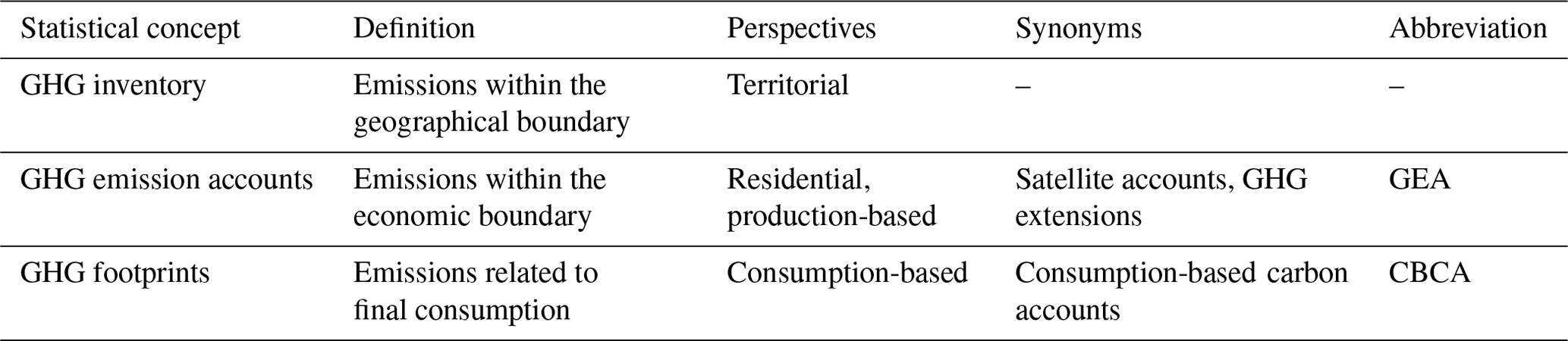
We estimate the uncertainty of the GHG emission accounts, thus leaving aside the uncertainty of the other two components of GMRIOs, i.e. the inter-industry matrix and final demand. GHG emission accounts are also referred to as GHG extensions or GHG satellite accounts (all three terms are used interchangeably in this work; see also Table 1). We focus on the GHG emission accounts for three reasons. First, inter-database comparisons identified the GHG emission accounts as the major source of discrepancy between difference GMRIO databases (Owen et al., 2016), which makes them a relevant starting point for improving the robustness of uncertainty estimates. Second, as detailed above, that is where we have authoritative information on raw data uncertainties, so that we avoid “guesstimating” them or basing them on (too) simplified assumptions. Third, as shown by Lenzen et al. (2010) and mentioned above, for carbon emissions the absolute size of a sector is an even poorer predictor of raw data uncertainty than for financial transaction. Thus, we expect that the inclusion of more robust raw data uncertainties will be especially relevant for GHG emission accounts.
We compile our own set of GHG emission accounts and estimate parametric uncertainty by using MC simulations to propagate the uncertainty from raw input data that enters the GHG extension compilation process to the GHG emission accounts and then further to the GHG footprints.
We compile the GHG emission accounts for the year 2015 according to the sectoral and regional resolutions of EXIOBASE V3 (Stadler et al., 2018) since it has the highest sectoral resolution of all currently available, harmonised (with respect to sector resolution) GMRIO databases. We cover the three major GHGs CO2, CH4 and N2O. As raw data for compiling GHG emission accounts, we follow recommendations by Tukker et al. (2018) and use, where available, emission data from the UNFCCC as a “robust, authoritative source” (Tukker et al., 2018). We base the analysis on the maximum entropy principle and thus try to use only the information that is available to use. Thus, we aim to provide a conservative baseline scenario of the uncertainty underlying the GHG emission accounts.
In addition to parametric uncertainty, we also provide an estimate of what Huijbregts (1998) calls “uncertainty due to choices”, reflecting the uncertainty that arises from decisions that inevitably have to be made in compiling and making use of GMRIO databases. Such decisions include for example the choice of the data sources used if there are several available (such as for GHG emissions) or the choice of how to allocate emissions to IO sectors. In GMRIO the uncertainty due to choices is either estimated specifically for one single decision using sensitivity analysis to study how the results differ when this decision is made differently (Wiebe and Lenzen, 2016; Schulte et al., 2021) or “generally” by comparing the outcome of different GMRIO databases (Owen et al., 2016; Tukker et al., 2018). Those inter-database comparisons allow one to study the variability in outcomes resulting from all decisions that have been made differently by the different database compilers in the course of compiling a GMRIO database. In this work, we choose the second approach by comparing our GHG emission accounts to those from other sources, i.e. the GHG emission accounts released by EXIOBASE V3.8.2 and official GHG emission accounts published by national statistical agencies and collected by the OECD.
By doing so, we aim to guide future GMRIO compilers to “uncertainty hotspots”, i.e. very uncertain data points which are relevant to answering a given research question, such that resources can be more efficiently guided to improve data accuracy (if parametric uncertainty prevails) or improve (align) the overall compilation procedure (if uncertainty due to choices prevails).
The aim of the study is twofold. First, we estimate and present the uncertainty of both GHG emission accounts (production-based perspective) and GHG footprints (consumption-based perspective), at two levels of detail – at the aggregate country level and the disaggregate sector level. Second, we provide GHG emission accounts along with their uncertainty to allow IO practitioners to conduct uncertainty assessment for their research question at hand.
In the following, Sect. 2.1 provides an overview of our methodology for compiling GHG emission accounts for EXIOBASE, including the raw input data and proxy data employed. Section 2.2 shows how we calculate GHG footprints using our GHG emission accounts along with data from EXIOBASE. Subsequently, Sect. 2.3 outlines our approach to modelling the uncertainty related to those GHG emission accounts, including the assignment of probability distributions to the input data (Sect. 2.3.1) and the propagation of uncertainty of the input data through the compilation process to derive uncertainty estimates for the GHG emission accounts and the GHG footprints (Sect. 2.3.2).
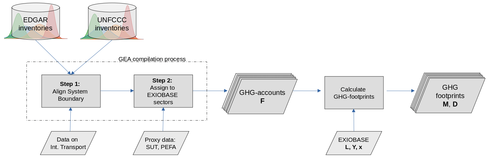
Figure 1Our workflow of propagating uncertainty from the raw input data sources (UNFCCC/EDGAR) to the GHG emission accounts and further to the GHG footprints.
2.1 Compiling GHG emission accounts
2.1.1 General information on GHG emission accounts
GHG emission accounts, also called GHG satellite accounts or GHG extensions (all three terms are used interchangeably in this work), represent GHG emissions broken down by emitting economic activity. Economic activities comprise both production and consumption activities. The System of Environmental-Economic Accounting (SEEA) provides the framework for the preparation of GHG emission accounts at the national level (UN et al., 2014). The SEEA framework shares the same system boundary as the purely economic System of National Accounts (SNA) to allow seamless integration between the economic IO tables (based on SNA) and the environmental extensions. As such, the GHG emission accounts list all GHGs emitted within the economic boundary of an economic unit such as a country, thus following the residential principle. According to the residential principle, national GHG emission accounts list all emissions caused by residence units of a country. A residence unit is an institutional unit (e.g. a corporation, household or general government) which “has its centre of predominant economic interest in a particular economic territory” (UN et al., 2014). Emission accounts present GHG emissions from the production perspective. The design of the system boundary is one major difference between GHG emission accounts and other emission statistics such as national emission inventories reported to the United Nations Framework Convention on Climate Change (UNFCCC), which follow the territorial principle listing all GHGs emitted within the geographical border of a country (see Table 1).
Two approaches for constructing GHG emission accounts can be distinguished: the inventory-first and energy-first approaches (Eurostat, 2015). Both differ in the raw data used in the compilation process. While the inventory-first approach starts with the ready-made emission inventories, in the energy-first approach energy accounts are constructed based on energy consumption data (such as the IEA World Energy Balances) and then combined with data on emission factors per fuel and economic sector. The energy-first approach ensures database-internal consistency between energy and emission accounts (Stadler et al., 2018) but at the cost of a lack of consistency with emission data from authoritative sources such as the UNFCCC. Hence, in this study, we follow the recommendations from a recent review of the robustness of GMRIO (Tukker et al., 2018) and use the inventory-first approach.
Thus, our approach differs from the EXIOBASE approach as of version 3.8.2. EXIOBASE compilers apply the energy-first approach by using IEA World Energy Balances to compile energy use accounts and then combine those energy use data with emission factors from the TEAM model (Stadler et al., 2018; Pulles et al., 2007). Thereafter, CO2 fossil emissions (until 2019) at an aggregate level are scaled to match EDGAR emissions and all other GHG emissions (until 2017) scaled to match the PRIMAP database (see the “README” files in Stadler et al., 2021). In Appendix A, we provide a figure of the different data sources used to compile selected GHG emission accounts and to show how they differ (Fig. A1).
Our workflow for the compilation of the GHG emission accounts and the calculation of GHG footprints is illustrated in Fig. 1. We construct GHG emission accounts following the guidelines as described in Eurostat (2015). We use GHG emission inventories as submitted to the UNFCCC and from EDGAR (Crippa et al., 2020b) as raw data input. We compile the GHG emission accounts according to the country and sector resolution of the industry-by-industry version of EXIOBASE V3, distinguishing 44 individual countries and five rest of the world (RoW) regions (see Table C1), each covering 163 industry sectors.
The GHG emission account compilation process can be divided into two major steps.
-
Step 1: aligning the system boundary to fit the residence principle
-
Step 2: assigning the emissions to EXIOBASE sectors
In the following, we first briefly describe the characteristics of the UNFCCC and EDGAR emission inventory data and then outline the two steps in the GHG emission account compilation process.
2.1.2 Emission inventory data
We base our analysis on the GHG emission inventories as submitted to the UNFCCC (hereafter referred to as UNFCCC data/inventories) and emission inventories from the Emissions Database for Global Atmospheric Research (EDGAR). UNFCCC inventories are available for all Annex-I countries (or parties) consisting of 40 developed or industrialised countries and the EU. Reporting follows the IPCC 2006 guidelines (IPCC, 2006). The UNFCCC inventories as published by the UNFCCC secretariat were obtained from Pflüger and Gütschow (2020). For all non-Annex-I countries and a few Annex-I countries for which we had problems while extracting uncertainty data (see Sect. 2.3.1 and Table C1 in the Appendix), we use the emission inventories from EDGAR v5.0 (Crippa et al., 2020a) since they have a global coverage (231 countries plus bunker fuel emissions), they are published on a yearly basis, and, like the UNFCCC inventories, their reporting largely follows the IPCC 2006 guidelines. EDGAR data were obtained from Crippa et al. (2020b).
Both UNFCCC and EDGAR classify GHG emission sources according to the Common Reporting Format (CRF). While EDGAR uses the CRF as stated in IPCC (2006), the more recent UNFCCC inventories follow a slightly updated version (IPCC, 2019). In both CRF versions, emission sources are grouped into categories in a hierarchical order. In the case of UNFCCC inventories, the highest-ranked categories – also called sectors – are (1) energy; (2) industrial processes and product use; (3) agriculture; (4) land use, land use change and forestry (LULUCF); (5) waste and (6) other. Those sectors are further broken down into sub-categories, e.g. 1.A.1.a.i. The level of detail with regard to categories differs between the UNFCCC and EDGAR data as well as between different countries. While EDGAR distinguishes only up to 22 different sub-categories, the national inventories submitted to the UNFCCC are much more granular, distinguishing up to 160 different sub-categories.
Furthermore, in the case of the UNFCCC inventories, the sub-categories of the energy, agriculture and LULUCF sectors are further broken down by the so-called classification. The classification distinguishes between different fuel types (in the case of emission from “Energy”) and animal types (in the case of emissions from “Agriculture”). Like the categories, the classification also follows a hierarchical structure, with a varying level of detail between individual country submissions. Hence, while for a certain category some countries only publish emissions from “liquid fuels” or even only the “total for category”, other countries distinguish between e.g. “gasoline” and “diesel”. EDGAR, on the other hand, does not provide details on the fuel or animal type.
We exclude emissions from LULUCF as they are commonly not included in air emission accounts due to a lack of detailed enough data to allocate those emissions to the industry and product sectors (Eurostat, 2015). Recently, efforts have been made to include LULUCF emissions in carbon footprint analysis (Hong et al., 2022). Further research could include those in the uncertainty analysis framework presented here.
2.1.3 Step 1: aligning the system boundary
As outlined above, emission inventories and emission accounts differ in their system boundary: while the former follows the territorial principle, the latter follows the residential principle. While a residence unit such as a company operates in most cases within the domestic territory, the exceptions can account for a considerable share of total national GHG emissions, especially for smaller economies like Luxembourg, Malta or Cyprus (Usubiaga and Acosta-Fernández, 2015). Consequently, a crucial step in compiling GHG emission accounts is aligning the system boundary from the territorial to residential principle, which is referred to as the “residence adjustment” (Eurostat, 2015). It should be noted, however, that not all global MRIO databases undertake this step (e.g. Eora (Lenzen et al., 2013) and ICIO (Wiebe and Yamano, 2016); see also Fig. A1 in the Appendix), which was found to be a major reason for the relatively large inter-database variability stemming from the GHG emission accounts (Owen et al., 2016).
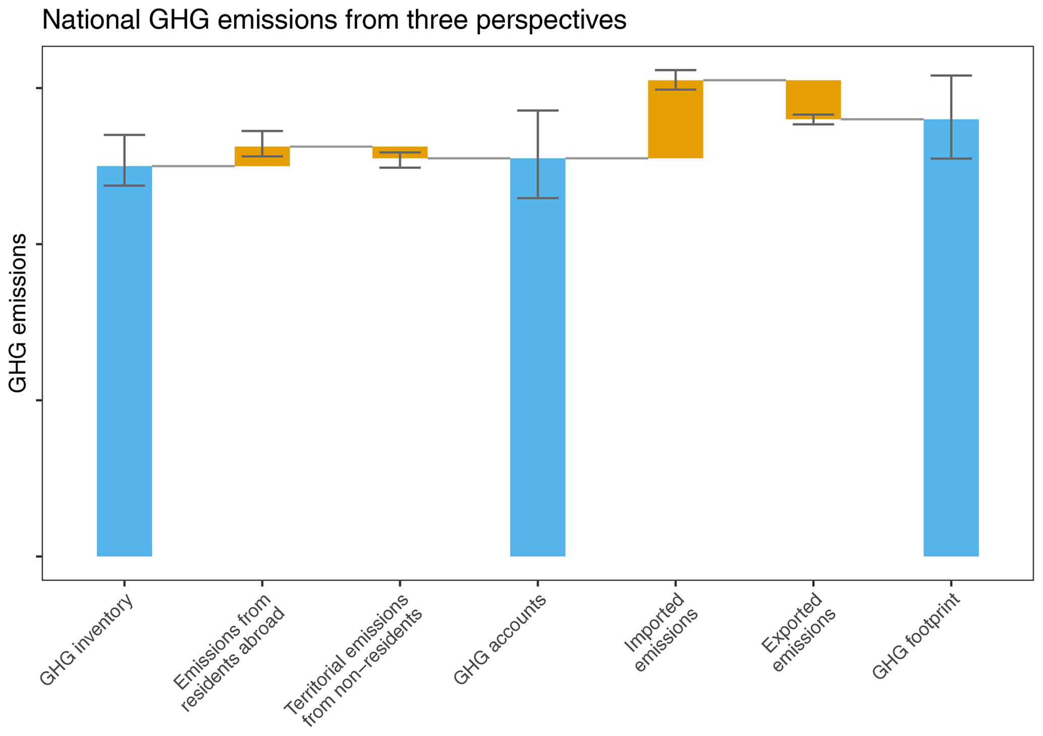
Figure 2Schematic waterfall plot showing the relations between the three different statistical perspectives on GHG emissions. Error bars illustrate that each component is subject to uncertainty.
The residence adjustment requires for each country or region (1) to deduct the emissions from non-resident units operating on the country's national territory and (2) to add the emissions from resident units operating abroad (see Fig. 2). These operations are explicitly presented in the so-called “bridging items”, which cover both deduction and addition operations for all relevant sectors. Thus, the net bridging items show the difference between national totals of territorial-based UNFCCC and EDGAR inventories and of national residence-based GHG emission accounts.
The residence adjustment affects a wide range of emission sources. However, due to the lack of data, estimating the bridging items is often hard. We therefore follow the compilers of EXIOBASE and WIOD and carry out the residence adjustment for the following globally relevant emission sources.
-
International air transport
-
International navigation
-
International fishing activities
-
International road transport
We note that for some individual countries there might exist other quantitatively relevant items (e.g. pipeline transport). However, conducting individual residence adjustments for each country is beyond the scope of our paper.
Emissions from international air transport, international navigation (shipping) and fishing activities have in common that they all occur, by definition, in international territory, i.e. in international airspace or in international waters. As emission inventories adhere to the territorial principle, these emissions are not included in national totals but are rather classified as “memo items”. Adding up all memo items from EDGAR delivers an estimate of the global total emissions from international air and maritime activities, respectively. Consequently, these memo items need to be added to the corresponding EXIOBASE sectors, i.e. “Air transport”, “Sea and coastal water transport” and “Fishing, operating of fish hatcheries and fish farms; service activities incidental to fishing”, of the countries that are home to the emitting institutional units. All emissions caused by the Irish airline Ryanair, for example, need to be added to the Irish air transport sector, because this is the sector where the purchases of the airline's customers will be recorded in the IO tables.
To ensure consistency with the total global emissions from international air and maritime activities from EDGAR, we calculate country-specific use shares for both activities using additional auxiliary data (details in Appendix D). Those use shares (which globally sum to 1) are multiplied by the total global international air or maritime emissions from EDGAR. In the case of international maritime activities, we calculate country-specific use shares using data from Selin et al. (2021). In their analysis, Selin et al. (2021) made a bottom-up estimate of the allocation of CO2 emissions from international shipping to national carbon budgets for the year 2015 using spatially resolved data on ship movements and ship-specific data on engine power demand, activity time and emission factor (details in Appendix D1). In the case of international air transport, we calculate country-specific use shares for EU countries using bridging items provided by Eurostat (Eurostat, 2022) and for non-EU countries using data from the World Bank on the country-specific numbers of domestic and international air passengers carried by air carriers registered in the country (Worldbank, 2023). For more details, see Appendix D2.
Emissions from international road transport occur within national territories but are caused by non-residence. As such, international road transport includes both tourism activities and road freight transport. These emissions need to be added to the corresponding EXIOBASE sector of the residence country of the emitter. For instance, emissions resulting from a tourist driving a car abroad would be allocated to the household sector of their home country. Similarly, emissions caused by a logistics company operating abroad would be added to the “Other land transport” sector of the country where the logistics company is registered. Moreover, as opposed to emissions from international territory, emissions from international road transport additionally need to be subtracted from the account of the country where the emissions occur (or more precisely from the country where the fuel was sold since emission inventories mostly use fuel sale statistics to estimate transport emissions).
In the case of international road transport, we follow Stadler et al. (2018) and consider the European countries to be by far the most affected by the residence adjustment of international road transport due to the European geography and its economic size (many countries in a relatively small area with a lot of cross-border commercial and recreational road transport). Non-European regions represented in EXIOBASE are “either islands or countries with limited road access in relation to their size (e.g. China, India)” (Stadler et al., 2018). We therefore assume that, for those countries, the road transport emissions from non-resident units operating on the country's national territory and the emissions from resident units operating abroad are the same. In other words, we assume the bridging items related to international road transport for non-European countries to be 0. However, in contrast to international air and water transport, we have no knowledge of the total (global or European) emissions from international road transport, as they are not reported separately as memo items but as part of the road transport sector emissions (CRF category 1.A.3.b) within each country. That is why – instead of calculating use shares as we do for water transport – we directly take the total bridging items from Eurostat (Eurostat, 2022) and add or subtract those from the respective EU country's national road transport emissions. Eurostat's bridging items do not sum to 0, and thus we distribute the residual to all European countries not listed in the Eurostat data using the total emissions from road transport (1.A.3.b) as a country-specific proxy. For details, please refer to Appendix D2.
2.1.4 Step 2: assigning emissions to MRIO sectors
Next to the differences in the system boundary, emission inventories and emission accounts also differ in their classification scheme. While inventories have more technical process-oriented classifications, emission accounts are grouped according to economic activity. Using the example of road transportation, in the UNFCCC CRF, emissions from road transportation are broken down according to emitting vehicle: cars, light-duty trucks, heavy-duty trucks, motorcycles and others, thereby focusing on differences in technology while ignoring the institutional unit that operates the vehicle, i.e. whether the operator is a household or transport company. In contrast, emission accounts would allocate these emissions from road transportation to the operators of the vehicles and thus to households, the logistics sector and all economic sectors that operate vehicles (which are basically all economic sectors; for details, see Appendix D3).
Creating a correspondence table (CT) is the first step in assigning the inventory emission sources to EXIOBASE sectors. The CT needs to map each combination of CRF category and classification (in the following referred to as a “CRF emission source”, e.g. “Liquid fuel” emission from category “1.A.1.a”), for each level of detail, to the EXIOBASE sectors differentiating between individual industry sectors and final demand categories. To get a CT that is consistent over all hierarchical levels, we manually constructed the CT for the most detailed combinations among all the countries (which we name “root classification”, following Lenzen et al., 2013). The upper level is then filled automatically by merging the respective EXIOBASE correspondences from the lower levels.
As a starting point, we take the correspondence table published by Eurostat that maps UNFCCC categories (without classification detail) to NACE rev2 sectors (until level 2, e.g. C11). Since we aim for a higher level of detail on both sides of the CT, considerable effort was needed to create the CT. We follow recommendations from Eurostat (2015) for creating correspondence tables by taking the following steps. First, we get a detailed understanding of the CRF categories and classifications (fuel and animal types) based on the IPCC 2006 guidelines (IPCC, 2006), EMEP and EEA (2019) and NIRs. Second, we get a detailed understanding of EXIOBASE sectors using the official documentation (Stadler et al., 2018, and the Supplement) and, where more detail is needed, the documentation of the NACE rev2 classification (on which the EXIOBASE classification is based). Third, we assign corresponding EXIOBASE sectors to each combination of CRF category and classification from the root classification. We end up with both 1-to-1 correspondences and 1-to-N (many) correspondences. Moreover, some CRF categories or classifications which are found to be country-specific are marked, and in a first step the correspondence is chosen according to the German inventory.1 Upcoming work could be to construct country-specific CTs (or even country-year-specific CTs, since correspondences within a country might also change over time). Since CRF emission sources marked as country-specific make up only a small share of the total emissions from Annex-I countries (0.4 % for CO2, 5.7 % for CH4 and 1.2 % for N2O), we consider our results to not be significantly affected by this pragmatic choice. Fourth, for each 1-to-N correspondence, we identify suitable proxy data to get a best-guess estimate for allocating (disaggregating) the CRF emission sources to MRIO sectors. As proxy data sources, we use in most cases the (monetary) Supply and Use Tables (SUTs) from EXIOBASE. To split emissions from Road Transport (CRF category 1.A.3.b) into EXIOBASE sectors, we use Eurostat's Physical Energy Flow Accounts (PEFAs) (Eurostat, 2023) along with the industry-sector-specific employment data from the EXIOBASE extensions (Stadler et al., 2018) as proxy data. Our CT including all UNFCCC–EXIOBASE mappings and their proxy data sources is available on Zenodo (see the Data availability section at the end of the paper).
Special case: road transport
Since road transport activities are undertaken by basically all industries and households, the allocation of emissions from road transport (CRF category 1.A.3.b) is one of the most difficult parts of compiling GHG emission accounts (Eurostat, 2015). Since the availability and quality of auxiliary data needed to estimate the shares of the respective industries and households in total road transport emission are highly country-specific (Eurostat, 2015), we use in a first step Eurostat's PEFAs to allocate road transport emissions to NACE rev2 industries and households for all EU28 countries plus Iceland and Norway (Eurostat, 2023). Given that a PEFA solely incorporates NACE rev2 industries up to the second level (e.g. C11), further disaggregation is needed to align with the more detailed sector classification of EXIOBASE. Consequently, in a second step, we further disaggregate emissions from NACE sectors to EXIOBASE sectors using sector-specific employment data from the EXIOBASE extensions (Stadler et al., 2018), more specifically the sum of the working hours from low-, middle- and high-skilled employment. In our analysis, we deem the total working hour input to be a more suitable proxy for allocating road transport emissions compared to the economic output of a sector. This choice is predicated on the assumption that the number of business trips (a major source of industry road transport emissions) is primarily contingent on the workforce size within a sector rather than solely relying on its overall output. For a more detailed and formal elaboration on how we allocate road transport, we refer the reader to Appendix D3.
2.2 Calculate GHG footprints
We transform the GHG emission accounts compiled with the procedure detailed above into a matrix F∗. The columns of F∗ represent the 7987 industry–country combinations following the structure of EXIOBASE V3, while the rows represent the 33 combinations of the three GHGs (CO2, CH4 and N2O) and 11 emission sources according to the UNFCCC CRF. By combining our GHG emission accounts F∗ with the other elements needed from EXIOBASE V3.8.2 (Stadler et al., 2021, 2018), i.e. the inter-industry coefficient matrix A, the sectoral output x and the final demand matrix Y, we first calculate the matrix of environmental multipliers M storing the consumption-based environmental impacts to produce one unit of output by industry sector:
where I is the identity matrix and is a square matrix with on the main diagonal and 0 elsewhere.
We calculate national footprints D as
2.3 Uncertainty analysis
We use MC simulations to propagate uncertainty from the raw data (GHG inventories from UNFCCC and EDGAR) to the GHG emission accounts and then further to the GHG footprints. Uncertainty propagation using MC requires us first to assign probability distributions to the raw input data. Subsequently, we perform MC simulations by repeatedly (N = 1000) and randomly sampling from those probability distributions. We use those N random samples to create a set of N GHG extension matrices following the procedure described in Sect. 2.1, which in turn are then used to calculate sets of N multiplier and of N national footprints (Sect. 2.2). In the following, we first show how we handle data uncertainty of the raw data and then explain in detail how we model uncertainty propagation.
2.3.1 Assigning probability distributions to input data
Uncertainties of national GHG emission inventories as submitted to the UNFCCC are available in the NIRs. NIRs are published annually by Annex-I countries along with the actual emission data (see Sect. 2.1.2). The reporting of the uncertainties in the NIRs largely adheres to the IPCC 2006 guidelines (IPCC, 2006), specifically the template table for uncertainty reporting found in Tables 3.2 and 3.3 of Vol. 1, Chap. 3. Since the NIRs are only available in pdf format, we first had to extract the uncertainty tables using a set of Python scripts. The extracted uncertainty estimates from the 2017 submission of UNFCCC NIRs covering the year 2015 are available on Zenodo (see the Data availability section at the end of the paper). Note that we were not successful in extracting uncertainty data for all Annex-I countries due to the lack of uncertainty data in those countries' NIRs or other issues which inhibited extraction or processing of those data. In Table C1 we list all EXIOBASE countries and regions, along with the database we used as a raw data source.
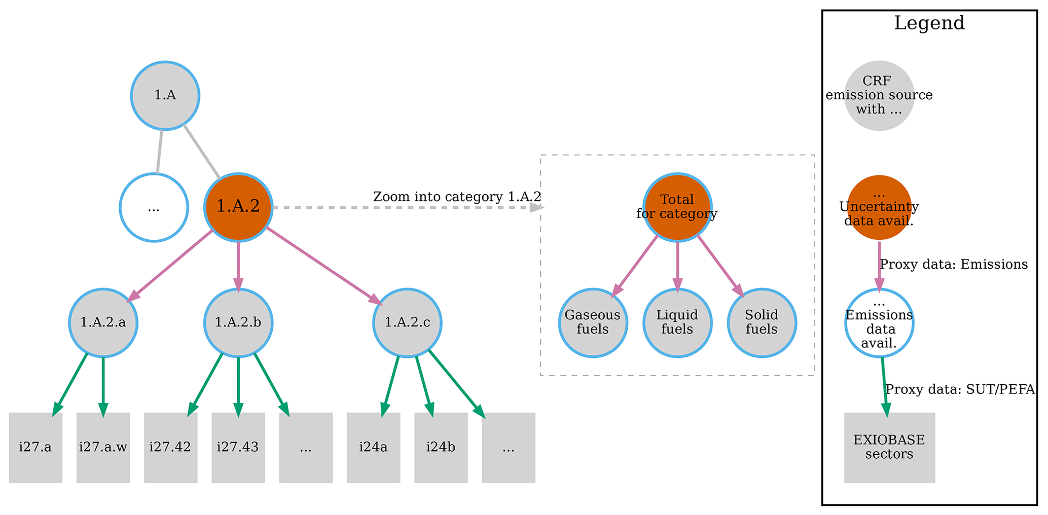
Figure 3An example of the nested hierarchical data structure of the UNFCCC inventories, one hierarchy on the left side representing the categories (e.g. 1.A.2 represents emissions from “Manufacturing Industries and Construction”). Each node representing a category contains another hierarchy representing the classification (i.e. fuel or animal type).
The NIR uncertainty tables list the uncertainties by source category (e.g. 1.A.3) and classification (i.e. fuel and animal types). The uncertainties are given either as one value representing a symmetric 95 % confidence interval (CI) around the mean (2 relative standard deviations: 2σ) or lower and upper uncertainty bounds which enclose the 95 % CI in the form (Q0.025,Q0.975), where Q0.025 and Q0.975 are the 2.5th and 97.5th percentiles, respectively. The type of uncertainty reporting depends on whether the reporting country estimated the emission uncertainties based on analytical error propagation where uncertainty in emissions is propagated from uncertainty of the activity data, emission factors and other parameters using the error propagation equation (Ku, 1966) (approach 1) or based on Monte Carlo simulations (approach 2; see IPCC, 2006).
For EDGAR data, which we use for all non-Annex-I countries and those Annex-I countries for which we could not extract the data from the NIRs, uncertainties are available from Solazzo et al. (2021). Solazzo et al. (2021) apply a similar approach by also following the IPCC 2006 guidelines (IPCC, 2006). Compared to the uncertainties reported by the UNFCCC, however, they mostly use default emission factor uncertainties from IPCC (2006), thus omitting national peculiarities. Like the uncertainty data from NIRs, Solazzo et al. (2021) report the EDGAR uncertainties as either symmetric or asymmetric 95 % CIs.
In the case of symmetric (approach 1) uncertainties, we assign a truncated normal distribution , where μ is the mean taken from the UNFCCC or EDGAR inventory data, σ is the standard deviation taken from UNFCCC NIRs or Solazzo et al. (2021), respectively, and a depicts the minimum value.
In the case of asymmetric (approach 2) uncertainties, we assign a log-normal distribution , where μ∗ and σ∗ are the mean and standard deviation of the variable's natural logarithm. μ∗ and σ∗ are both estimated, so that the 95 % CI of the log-normal distribution fits the 95 % CI, as given in UNFCCC NIRs or Solazzo et al. (2021) using the R package rriskDistributions (Belgorodski et al., 2017).
To examine how the “law of large numbers” which has been used in the literature (Lenzen et al., 2010; Karstensen et al., 2015; Zhang et al., 2019) performs for the uncertainty data from the UNFCCC and EDGAR, we fit power law regressions, both pooled and by country (Fig. E1 and Sect. E1 in the Appendix).
One major challenge for both emission inventories (UNFCCC and EDGAR) is that the level of detail of the uncertainty data often does not match the level of detail of the emission data. This mismatch in resolution is present in both categories (i.e. processes and sectors) and classifications (i.e. fuel and animal types, applicable to the UNFCCC only since EDGAR does not distinguish between fuel and animal types).
Figure 3 exemplifies this mismatch for the CRF category 1.A.2 comprising emissions from fuel combustion from “Manufacturing Industries and Construction” and its sub-categories. In that example, we have emission data up to the fourth category level (1.A.2.a Iron and Steel, 1.A.2.b Non-Ferrous Metals, etc.), each for three different fuel types (see the circles outlined in light blue). Uncertainty data, however, are only available at the third category level (1.A.2) without any details on fuel type (see the circles filled in orange). The easy solution to deal with this mismatch in granularity would be to use the data at the level of detail for which both emission and uncertainty data are available. This option, however, would come at the cost of losing valuable information on the composition of the emission sources, so that we would have to make even more assumptions regarding the allocation of emissions to MRIO sectors. As such, in order to use all the information available, we handle the data in a hierarchical tree format, in two different variants based either on (A) the category or (B) the classification, so that we have one data tree for each party, year, gas and classification (in the case of A) or one data tree for each party, year, gas and category (in the case of B), respectively. We wrote functions to flexibly reshape the data between the usual table format and the category or classification tree formats.
The modelling of uncertainty of the residence adjustment (Sect. 2.1.3) differs between international road transport on the one hand and international air and water transport on the other hand. While in the case of the former we have no information on the total (global) emissions from international road transport but only on the country-specific bridging items, in the case of the latter we know the total (global) emission from international air and water transport from the UNFCCC and EDGAR memo items (see Sect. 2.1.3) along with their uncertainties (see the next section).
That is why, for international road transport, we explicitly need to assign uncertainty estimates to the country-specific bridging items, while for international air and water transport we can model the uncertainty of the country-specific bridging items by disaggregating the global international air or navigation emissions using the procedure presented below. Since Eurostat does not provide uncertainties of their bridging items, we assume a relative standard deviation of 0.3. Note that, due to taking totals (instead of use shares), the uncertainty propagation also differs between the residence adjustment related to international road transport as opposed to emission happening in international territory.
2.3.2 Propagating uncertainty
We propagate the uncertainty using 1000 MC simulations in three steps:
-
from the nodes that have uncertainty information (Fig. 3, orange circles) to the most detailed level to which emission data are available (Fig. 3, lowest-level blue-bordered circles);
-
from these inventory leaves further to the MRIO sectors (extensions); and
-
from the GHG emission accounts to the GHG footprints.
The aforementioned Fig. 3 illustrates steps (1) and (2) of the uncertainty propagation procedure. Steps (1) and (2) involve both 1-to-1 mappings (i.e. a node is only connected to one lower-level node, not shown in Fig. 3) and 1-to-N mappings (i.e. a node is connected to two or more lower-level nodes). While the first case is trivial, the second one involving data disaggregation requires further attention.
The problem of data disaggregation under uncertainty (i.e. in a probabilistic framework) appears in many different research fields (e.g. chemistry: Plessis et al., 2010; economics: Rodrigues, 2014; energy statistics: Paoli et al., 2018, Min and Rao, 2018). The main characteristic of the problem of data disaggregation is the preservation of the accounting identity, i.e. the constraint that all disaggregate data values need to sum to the aggregate data value x0:
Rewriting Eq. (3) by substituting gives
where αi is the branching ratio (or sector share) of sector i, and . The accounting identity constraint naturally introduces negative correlations between the αis (Rodrigues, 2016).
We approach the problem of data disaggregation under uncertainty as follows: first, we sample the aggregate from the uncertainty distribution for x0 assigned in Sect. 2.3.1. Second, we sample the disaggregate branching ratios from the Dirichlet distribution of , which will be detailed in Schulte et al. (2024). Together, and α′ then provide the sampled disaggregate values: .
For data disaggregation in a probabilistic framework, the Dirichlet distribution is often a natural choice (see Paoli et al., 2018, e.g.), since it has the helpful properties that random variables drawn from the distribution always sum to 1. Formally expressed, the Dirichlet distribution describes K≥2 random variables such that each and . The Dirichlet distribution we use which is described in Plessis et al. (2010) is parameterised as follows:
where is a vector of positive-valued parameters such that and an additional positive-valued concentration parameter γ>0. The Dirichlet distribution, as described here, has the useful property that the expected values for each variable Xi equal the parameter value αi:
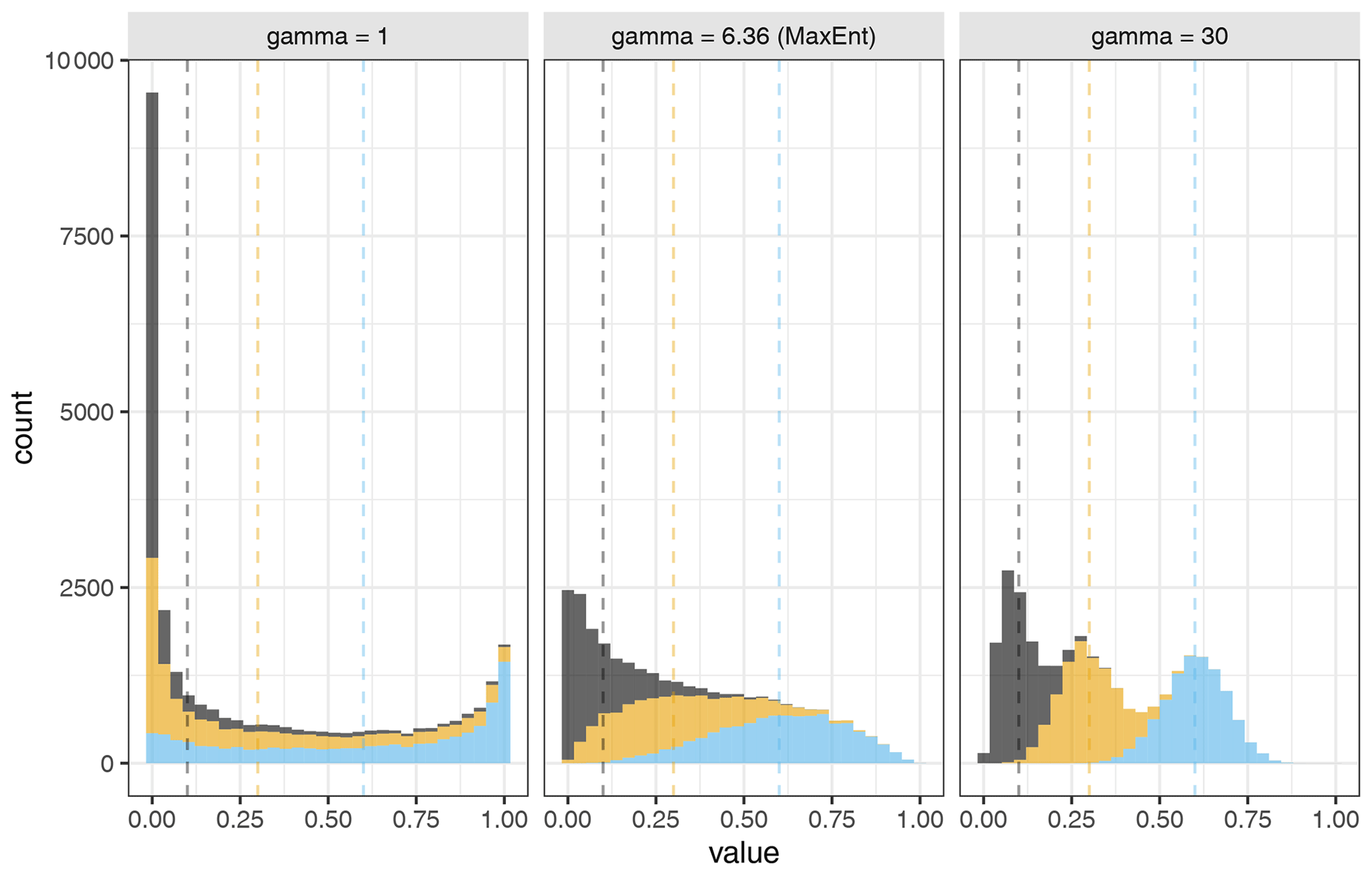
Figure 4Histograms of sector shares for three sectors (grey, yellow, blue) sampled from Dirichlet distributions with different values of gamma (N = 10 000, , ).
The concentration parameter γ, on the other hand, controls the variance of X. This is illustrated in Fig. 4, showing histograms of 10 000 random numbers generated with three different Dirichlet distributions, all with the same average sector shares but with different values of γ. From the figure, we can see that the variance decreases with increasing γ.
In other words, with the parameter γ we can introduce uncertainties of the sector shares. However, we have no information on how accurate the SUT and PEFA data are as a proxy for disaggregating emission data. Thus, without quantitative information uncertainties of the sector shares, we cannot choose one of these realisations of the Dirichlet distribution without explicitly making an (arbitrary) assumption about the uncertainty (i.e. variance) of the shares. Against this background, the maximum entropy (MaxEnt) principle provides a powerful framework to deal with all available information and constraints in a consistent manner. According to Jaynes (1957), from all probability distributions that align with a given set of constraints and information, the one with the maximum entropy should be selected. The MaxEnt principle implies that the chosen distribution is at the same time maximally uninformative about what is unknown and maximally informative about what is known. Consequently, the MaxEnt distribution provides the least biased estimation that remains consistent with the provided constraints and information. Thus, in our case we want to find the least informative – or least biased – Dirichlet distribution with given sector shares α. More precisely, we estimate the concentration parameter γ such that the entropy of the Dirichlet distribution Dir(α;γ) is maximised. A more detailed elaboration of our procedure is under preparation (Schulte et al., 2024).
Here, we present the results from propagating uncertainties from the UNFCCC and EDGAR emission inventories to the GHG emission accounts and further to the GHG footprints. The Results section is structured as follows. First, Sect. 3.1 shows the uncertainty of the GHG emission accounts and the GHG footprints at the level of countries or regions and compares our range estimates to the point estimates from the official EXIOBASE GHG emission accounts and – if available – GHG emission accounts published by national statistical offices (and collected by the OECD). Subsequently, Sect. 3.2 shows the uncertainty at the level of industry sectors.
We provide the 95 % CI [Q0.025,Q0.975] depicting the interval between the 2.5th and 97.5th percentiles of the 1000 Monte Carlo samples.
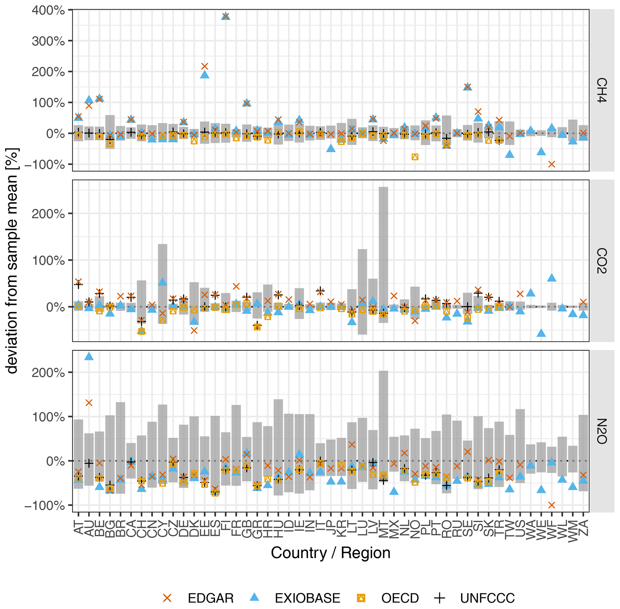
Figure 5Uncertainty of the GHG emission accounts for the 49 EXIOBASE countries and regions, shown as the relative deviation from the sample mean. Grey bars show our 95 % CI. The blue and yellow points show the relative deviation of the official EXIOBASE V3.8.2 emission accounts and the collection of national emission accounts from the OECD, respectively, from our sample mean. EDGAR and UNFCCC emission inventories (territorial-based) are additionally displayed to help explain some of the differences between our GHG emission accounts and those from the OECD or EXIOBASE. See Appendix C1 for a definition of all EXIOBASE country or region codes.
3.1 Uncertainty at the regional or country level
Figure 5 shows that the uncertainty of the GHG emission accounts at the country level for the three GHGs CO2, CH4 and N2O. The grey bars show the uncertainty as the relative deviation of the 95 % CI from the sample mean. For CO2, the uncertainties range between minimally [−2 %, +3 %] for the RoW region Middle East (WM) and maximally [−35 %, +257 %] for Malta (MT). For CH4, the uncertainties range between minimally [−8 %, +10 %] for RoW Europe (WE) and maximally [−50 %, +59 %] for Bulgaria (BG). For N2O, the uncertainties range between minimally [−26 %, +34 %] for RoW Middle East and maximally [−48 %, +203 %] for Malta. Thus, the uncertainty ranges span almost a factor of 100 for CO2 and less than a factor of 10 for N2O and CH4. Moreover, for most countries, the 95 % CI is positively skewed. This can be explained by the constraint that emissions can only be positive, and thus the theoretically maximum relative downward deviation from the mean is −100 %.
Comparing our range estimates to the point estimates from the official EXIOBASE GHG emission accounts and the collection of national emission accounts from the OECD (coloured points in Fig. 5, summary statistics in Fig. E2 in the Appendix), we observe that, for most countries, both EXIOBASE and OECD estimates fall within our 95 % CI. Exceptions include some countries (AT, AU, BE, EE, FI, GB, HU, PT and SE; see Table C1 for the country codes) for which the CH4 estimate from EXIOBASE is well above our 95 %, in the case of Finland (FI) even by a factor of more than 3. We suspect that those discrepancies can mostly be explained by the different source data used, which for those countries also differ considerably. While EXIOBASE estimates align well with the EDGAR inventory data (see Sect. 2.1.1 for details on the way EXIOBASE compiles its GHG accounts), our estimates and OECD estimates are both based on the UNFCCC inventories. Therefore, we conclude that, for those countries, the uncertainty due to choices (in this case the choice of database) is much higher than the parametric uncertainty.
Also in the case of the four EXIOBASE RoW regions, EXIOBASE estimates mostly fall outside our 95 %. This might result from the fact that, in contrast to most countries that are individually present in EXIOBASE, there is no official “benchmark” estimate for the emissions of those RoW regions. In the case of the CO2 emission accounts from Switzerland (CH) and Sweden (SE), both EXIOBASE and OECD estimates are below our 95 % CI. In the case of N2O, we observe that for most countries the EXIOBASE and OECD estimates are systematically below our sample mean (but still within our 95 %). An exception to that is Australia (AU), where EXIOBASE reports 250 % higher (residential-based) N2O than our sample mean. However, similar to the CH4 “outlier”, we also suspect the different source data of being (one) explanation for this discrepancy.
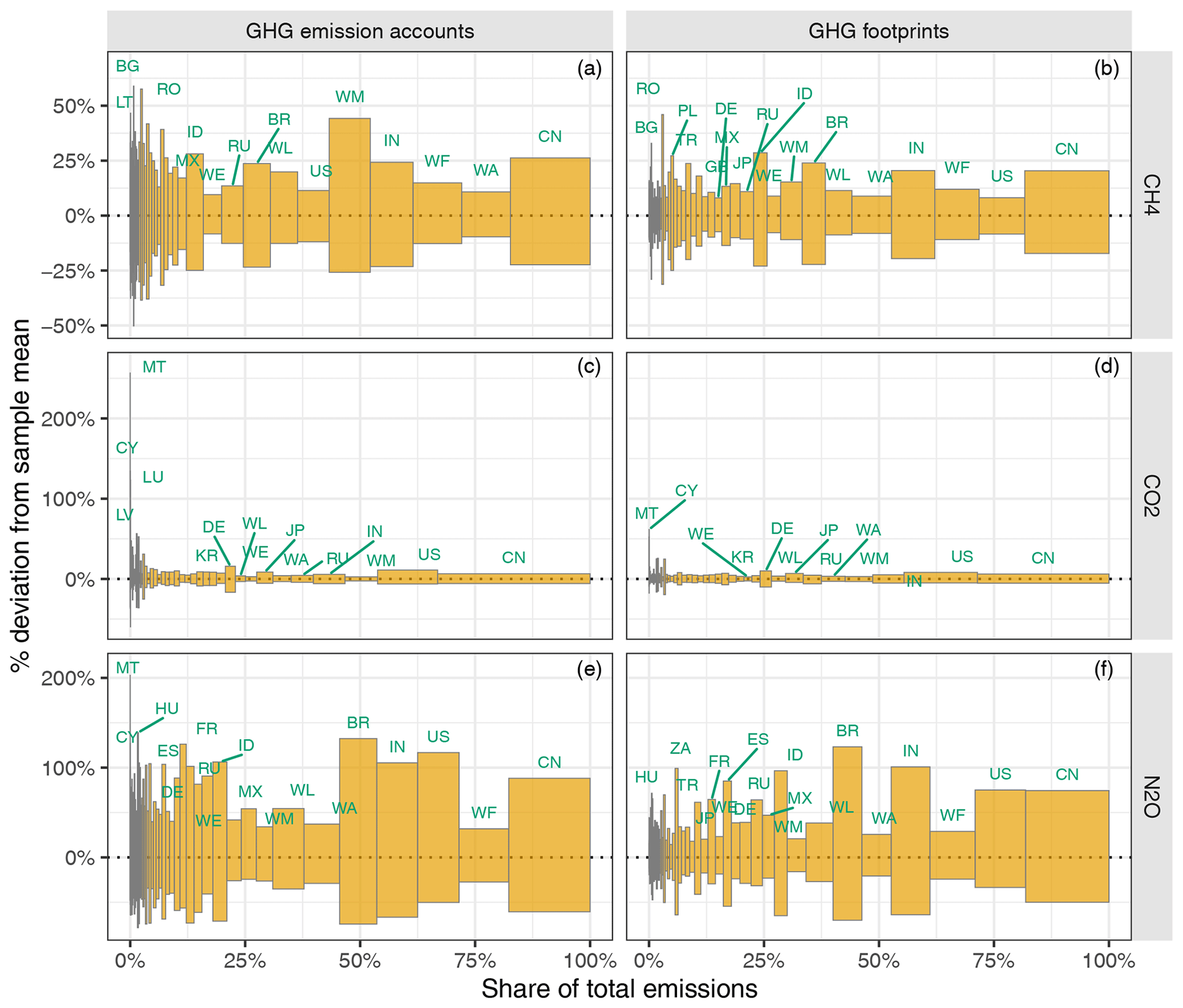
Figure 6Uncertainty of the GHG emission accounts (a, c, e) and of the GHG footprints (b, d, f) at the country or region level, shown as the relative deviation from the sample mean. The yellow bars show our 95 % CI. Countries are sorted along the x axis according to their mean share of the total emissions. The bar width is adjusted to the mean share of the total emissions. For EXIOBASE, country or region codes, see Table C1.
Figure 6 displays the uncertainties of the GHG emission accounts next to the uncertainties of the GHG footprints, allowing one to analyse how the uncertainty propagates from the production-based GHG emission accounts through international supply chains to the consumption-based GHG footprints. This time, the countries are sorted along the x axis according to their mean share of total emissions (according to our estimate).
Focusing on the uncertainty of the GHG emission accounts (Fig. 6a, c and e), we see that, in the case of CH4 and N2O, there is no clear trend between a country's emissions' uncertainty and its absolute emissions. This means that the uncertainty is relatively uniform between countries, regardless of the size of their total emissions. In contrast, for CO2, a clear trend emerges where countries with larger overall GHG emission accounts exhibit lower uncertainty. Those countries with by far the greatest uncertainty – MT, Cyprus (CY) and Luxembourg (LU) – all have very small (production-based) contributions to global CO2 emissions. Countries and regions with a considerable contribution to global CO2 emissions, on the other hand, such as China (CN), the US, RoW Middle East (WM) or India (IN), show relatively small uncertainties, with CIs all ranging within the interval [−10 %, +10 %].
Comparing the uncertainty of the GHG emission accounts (production-based) to the uncertainty of the GHG footprints (consumption-based), we observe that for most countries the uncertainty of the former is considerably higher than of the latter. This can also be seen in Table 2, which shows the distributions of the coefficients of variation (CVs) as the median (50th percentile) and the 2nd and 97.5th percentiles.
Table 2Distribution of the coefficients of variation (CVs) of the country- and sector-level GHG emission accounts and GHG footprints. Numbers are denoted in the form of .
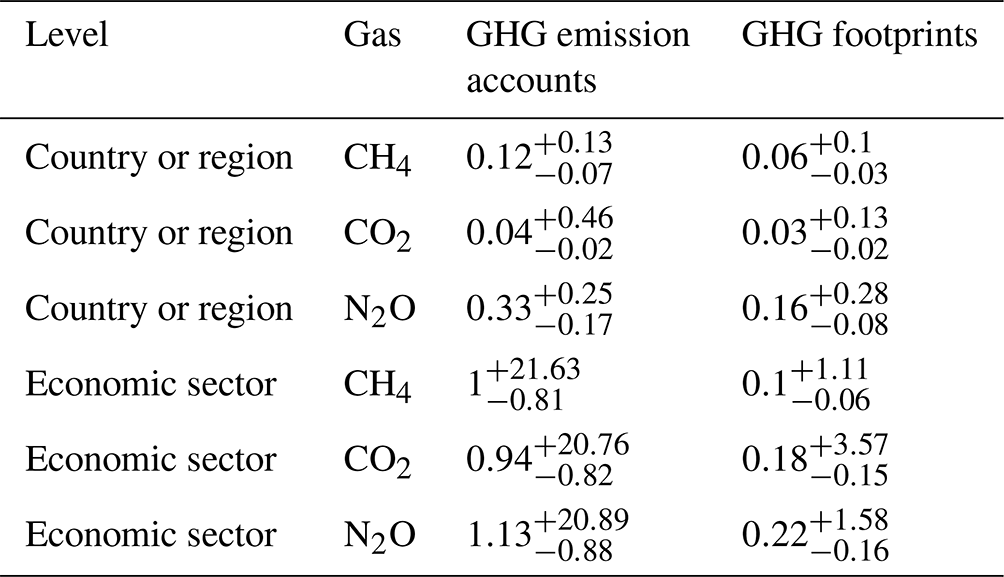
This difference is particularly striking in countries with very uncertain GHG emission accounts, such as Malta and Cyprus, especially concerning CO2 and N2O emissions. The lower uncertainty in GHG footprints compared to GHG emission accounts can be attributed to the fact that, when calculating footprints, the emissions from GHG emission accounts – and their associated uncertainties – are distributed internationally through global supply chains. For example, a large share of Malta's “sea and coastal water transport” services, whose emissions are a major source of uncertainty (see Fig. E3 in the Appendix), is not consumed domestically but relates to final consumption in other parts of the world. However, it must be noted that, in our analysis, we only consider the uncertainty of the GHG emission accounts, thus neglecting the uncertainty stemming from all inter-industry flows, including how emissions are internationally distributed through global supply chains. Hence, depending on the sizes of those uncertainties not covered here, the ratio might also be reversed.
3.2 Uncertainty at the sectoral or multiplier level
Next, we turn to the uncertainty at the level of industry sectors. The industry-by-industry version of EXIOBASE V3.8.2 covers 163 economic sectors in each of the 49 countries and regions, resulting in a total of 7987 economic sectors. We analyse both the uncertainty of the sectoral GHG emission accounts and the uncertainty of the sectoral GHG footprints. In the case of sectoral GHG footprints, the consumption-based emissions to produce one unit of output are also often referred to as the (emission) multiplier.
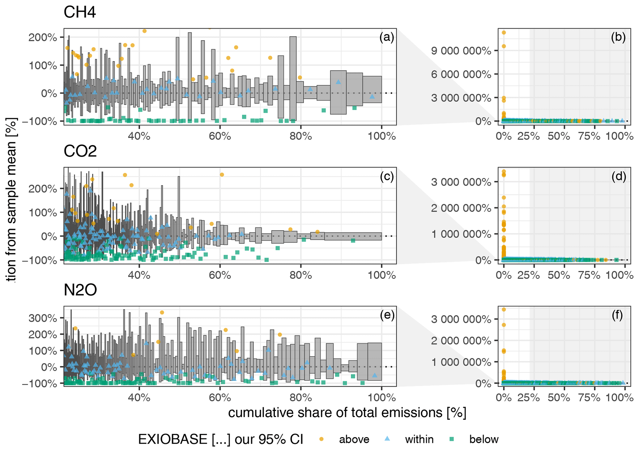
Figure 7Uncertainty of the GHG emission accounts for the 7987 EXIOBASE sectors against their cumulative share of the total emissions. The right column (b, d, f) shows all the sectors, and the left column (a, c, e) zooms into those sectors covering the top 80 % of the total emissions. Uncertainty (y axis) is shown as the relative deviation from our sample mean. Grey bars display our 95 % CI, with the width being adjusted to the mean share of the total emissions. The coloured points depict the EXIOBASE V3.8.2 estimate for that sector. The colours indicate whether the EXIOBASE estimate is above, below or within our 95 % CI. Sectors are sorted along the x axis according to their mean share of the total emissions. Note: sectors with zero emissions are not displayed.
Figure 7 displays the uncertainty relative to the mean in the (production-based) GHG emission accounts of those economic sectors. Each economic sector is represented by one grey bar showing the range of its 95 % CI (y axis) and its share in total (global) emissions (x axis). The sectors are sorted along the x axis according to their mean share of total emissions. The coloured points depict the EXIOBASE V3.8.2 estimate for that sector. Colours indicate whether the EXIOBASE estimate is above, below or within our 95 % CI.
Figure 7b, d and f show all the sectors (except those with zero emissions). From there we can see that, for some sectors with a very small contribution to the total emissions, the EXIOBASE estimates deviate substantially by up to a factor of +1 × 10⁹. However, since those sectors only make a very small contribution to global emissions but completely dominate the scale of the y axis, we zoom into those sectors which cover the top 80 % of the total emissions (Fig. 7a, c and e). For those top-80 % sectors, the 95 % CI ranges between [−100 %, +200 %] for CH4, [−100 %, 300 %] for CO2 and [−100 %, 350 %] for N2O.
For CO2, similar to the country-level uncertainties, a clear trend can be observed between a sector's emission uncertainty and its absolute emissions. For example, the 95 % CIs of the sectors covering the top 40 % of the total CO2 emissions are all within [−50 %, +50 %], while for N2O the sector with the highest share of total emissions (China – cultivation of vegetables, fruit and nuts) shows a 95 % CI of [−85 %, 140 %], and for CH4 the sectors with the third-highest share of the total emissions (China – mining of coal and lignite; extraction of peat) show a 95 % CI of [−70 %, +90 %]. Moreover, like for country-level uncertainties, for most sectors the 95 % CI is positively skewed.
Comparing our range estimates (covering the 95 % CI) with the point estimates from EXIOBASE, we see – in contrast to the country-level results – a considerable deviation between the EXIOBASE estimates and our 95 % CIs (coloured points in Figs. 7 and E2 in the Appendix). All sectors for which the EXIOBASE estimate falls within our 95 % CI make up 28 % (CO2), 35 % (CH4) and 41 % (N2O), respectively, of global emissions (see Fig. E2 in the Appendix). For most sectors, making up 58 % (CO2), 47 % (CH4) and 53 % (N2O) of the total emissions, the EXIOBASE estimate is below our 95 % CI, while sectors for which EXIOBASE provides higher emission values make up 14 % (CO2), 17 % (CH4) and 6 % (N2O) of global emissions. Therefore, we conclude that the uncertainty due to choices outweighs the parametric uncertainty for most sectors, or, put differently, all choices made differently between us and the compilers of the official EXIOBASE GHG emission accounts (see Sect. 2.1.1 for details on the way EXIOBASE compiles their GHG accounts) affect the sector-level emission accounts more than the raw data uncertainties. Tables E1 and E2 in Appendix E2 list all EXIOBASE sectors for which our sample means are considerably (i.e. for more than 75 % of all the regions) above or below the official EXIOBASE V3.8.2 estimate, thus shedding light on sectors for which the process of emission assignment (Sect. 2.1) needs further investigation in terms of proxy data used or incorrect correspondences from raw data items to those sectors.
Comparing the uncertainty in GHG emission accounts with those of the GHG footprint, we see that, overall, the uncertainty is substantially lower for the latter. This is indicated by the boxplots in Fig. E4 in the Appendix and the summary statistics in Table 2). From Table 2 we see that the median CV is a factor of 5 to 10 lower for the sector-level GHG footprints than for the sector-level GHG emission accounts. This finding is in line with the results at that country level and can also be explained by the fact that, in the footprint calculations, uncertainties are distributed internationally through global supply chains, where they partly cancel out.
4.1 Uncertainty of GHG accounts at the country level
In our analysis, we estimate the uncertainty of the GHG emission accounts by propagating uncertainty from the raw data inputs needed to compile them, i.e. the GHG inventories, to the accounts. In doing so, we identify several uncertainty hotspots. At the country level, countries with small economies and comparably little GHG emissions exhibit higher uncertainties than large economies with large emissions, a pattern that is strongest for CO2 emissions, in which case the pattern can mostly be attributed to the residence adjustment (see Fig. E3 in Appendix E). In the residence adjustment, large chunks of emissions are allocated across many countries. Since we model this allocation using a maximally uninformative Dirichlet distribution, the amount of emissions attributed to a specific country shows a high variability. For countries like Malta or Cyprus, where the international aviation and/or shipping sector play a considerably high role in overall economic activities, this uncertainty also contributes considerably to the uncertainty of the national GHG emission accounts. For large economies like China or the US, on the other hand, these sectors play – in relative terms – an almost marginal role; therefore, their overall uncertainty remains relatively unaffected by the uncertainty of the residence adjustment.
Comparing our range estimates with EXIOBASE and OECD point estimates at the country level, we observe that, for the majority of countries, both the EXIOBASE and OECD point estimates are encompassed within our 95 % confidence interval. To conclude, GHG emission accounts at the country level appear reasonably accurate, especially for CO2 emissions, provided that international transport emissions are a minor component in comparison to the broader economic activities of a country. However, caution is warranted: disparities between our estimates and those from EXIOBASE and the OECD exist for specific countries (like Switzerland, Romania or Sweden) and some RoW regions, emphasising the importance of choices made while compiling GHG extensions, such as the source data selection (UNFCCC vs. EDGAR), the approach applied (inventory-first vs. energy-first), the elaboration of correspondences between emission categories and economic sectors, and proxy data selection.
Furthermore, the CH4 and N2O emission accounts demand a more cautious interpretation. They possess considerably higher parametric uncertainties, primarily due to the higher uncertainty in raw inventory data (Solazzo et al., 2021). Additionally, the uncertainty resulting from choices, particularly concerning the raw data source (EDGAR vs. UNFCCC), is substantial. For CH4, choosing between EDGAR or UNFCCC can lead to deviations as large as 300 % for some countries. For N2O, a clear trend emerges: our method frequently produces higher estimates compared to EXIOBASE or the OECD. This recurring variance necessitates further investigation to determine its root causes.
4.2 Uncertainty of GHG accounts at the sector level
At the sector level, the uncertainty significantly surpasses that of the country level, with CVs reaching values of up to 10. For CO2, uncertainties are distributed unevenly. Larger sectors, in terms of emissions, typically display less uncertainty. However, for CH4 and N2O, the uncertainties are comparatively uniform across industries. Consequently, for CH4 and N2O, even sectors with high emissions exhibit considerable uncertainty. When juxtaposed with the estimates from EXIOBASE at the sector level, the alignment is less consistent than at the country level. On average, EXIOBASE estimates tend to be below our 95 % CIs, while for certain sectors with relatively low emissions, the EXIOBASE estimates show considerable upward deviations.
In conclusion, for GHG emission accounts at the sector level, CO2 estimates for sectors with large emissions seem reasonably accurate. However, substantial uncertainties in CO2 emissions exist for sectors with rather low overall emissions and for CH4 and N2O emissions in general. This suggests that a more cautious interpretation is warranted for these sectors and emissions. This heightened level of overall uncertainty at the sector level resonates with findings from other studies (Lenzen et al., 2010; Karstensen et al., 2015; Rodrigues et al., 2016) that have also highlighted the need to approach individual data items in a GMRIO database with caution.
Furthermore, the uncertainty due to choices (see Huijbregts, 1998, and Appendix B) is predominant at the sector level. A significant proportion of the sectors in terms of both number and emission size fall outside our 95 % CI, implying that all choices made differently by us as compared to the EXIOBASE compilers have a greater impact on the sectoral variability than the parametric uncertainty. Consequently, to enhance the robustness of sector-level emission accounts, there is a need for a more systematic analysis of the uncertainty that results from different choices made in compiling GHG emission accounts. The aspects needed to be considered in such an assessment include industry correspondences, residence adjustments and the nature of the proxy data utilised (see also Appendix E2).
4.3 Uncertainty of GHG footprints
In our analysis, we also show how the uncertainty propagates further from the GHG emission accounts to the GHG footprints. We find that, overall, production-based emission accounts exhibit higher uncertainty than consumption-based accounts (GHG footprints). This is especially pronounced for sectors with high uncertainty in production-based emissions. This finding can be explained by the fact that, when calculating footprints, the production-based emissions along with their uncertainties are distributed internationally through global supply chains to serve final consumption in another part of the world. Since we assume the uncertainties of the production-based emission accounts to be uncorrelated (except those stemming from a common raw data point; see Sect. 2.3.2), we expect them to partially cancel out each other when propagated through the supply chains, resulting in a lower uncertainty of GHG footprints. However, in our analysis we do not include the uncertainty of the entries in the inter-industry coefficient matrix A, the sectoral output x and the final demand matrix Y (see Eq. 1). Therefore, depending on the magnitude of these uncertainties and the structure of the correlations we did not cover, consumption-based emission uncertainties might indeed be even higher than the uncertainties from production-based emissions.
4.4 Assumptions, limitations and outlook
This analysis provides a conservative baseline scenario of the parametric uncertainty inherent in GHG emission accounts. Thus, we only – with one exception (see below) – include estimates of raw input data uncertainty when it comes from authoritative sources and is available to us. In our case, both criteria are fulfilled by two data sources: the National Inventory Reports as submitted to the UNFCCC (Tukker et al., 2018, see) and the study by Solazzo et al. (2021) providing uncertainties for the EDGAR database based on the IPCC 2006 guidelines (IPCC, 2006). For most other raw input data where uncertainty estimates are not available, we assume maximally uninformative distributions or, in more technical terms, those distributions maximise the statistical entropy. This is especially true for all proxy data used to disaggregate and assign emission inventory data to the MRIO sectors. The only exception, in which we deviate from the maximum entropy principle, is for the bridging items used for the residence adjustment concerning international road transport. For these bridging items, we lack a (global) total emission estimate as compared to international air or water transport emissions. Thus, we need to make an explicit assumption about their uncertainty (see Sect. 2.3.1).
Further research could narrow down the uncertainty ranges of raw data inputs for which we used maximally uninformative prior distributions by either relying on expert judgement or using an approach similar to the pedigree matrix approach applied to the life cycle inventory database ecoinvent (Ciroth et al., 2016). This could be achieved by including uncertainty estimates to both proxy data to assign emissions from international transport (air, ship, fishing) to national GHG accounts in the so-called residence adjustment (Sect. 2.1.3) and the proxy data to assign emissions from GHG inventories to MRIO sectors (Sect. 2.1.4). The inclusion of uncertainty estimates of the proxy data would be possible in the framework proposed in this study but replacing the standard Dirichlet distribution as applied here with a generalised Dirichlet distribution such as the one formulated by Plessis et al. (2010) in order to “force” the disaggregate samples to stay within a given range.
Our analysis comes with several limitations, outlined as follows. In our analysis, following the classification by Huijbregts (1998), we have accounted for two types of uncertainty in GMRIO modelling: parametric uncertainty and uncertainty due to choices. While in the case of the former we have considerably advanced the state of the art in uncertainty estimation in GMRIO, in the case of the latter our analysis only provides a very general analysis of the uncertainty due to choices by comparing our GHG emission accounts to other databases which made a different set of choices or assumptions in their compilation process. Particularly in view of our finding that the uncertainty due to choices plays a major role in most sectoral emissions and some country emissions, a more systematic analysis of the uncertainty that results from different choices in compiling GHG emission accounts should be made. This could be achieved with a sensitivity analysis by varying one assumption or choice at a time (e.g. source data, proxy data or sector mapping) to identify the decisions with the largest sources of variability.
Moreover, we neglect other sources of uncertainty and variability, such as model or scenario uncertainty, spatial variability, temporal variability or variability between objects or sources (see Table B1 and the discussion in Appendix B). Especially the latter three sources of variability result in a variability in inputs and outputs (e.g. in forms of GHG emissions) within each GMRIO sector, which is hidden in the model due to the sector-homogeneity assumption (Majeau-Bettez et al., 2016). While this within-sector variability (also called the aggregation error) might be of less relevance at the country level due to effects of cancelling out, it might constitute a considerable source of uncertainty for analysis carried out at the sectoral level (“product footprints”) or at the sub-national level, e.g. in household footprint studies. When interpreting our results, it should be kept in mind that the uncertainty estimates we provide are on the mean emissions of that sector. However, depending on the characteristics of a sector, the within-sector variability might be substantially larger.
Moreover, there is a trade-off between the within-sector variability and the uncertainty of the mean with respect to the sectoral resolution: the more you aggregate sectors, the lower the uncertainty on the mean (due to cancelling-out effects, except when uncertainties are highly positively correlated) but the higher the within-sector variability. As shown by Lenzen (2011), IO-based results are more accurate if you first disaggregate the IO data, then perform the calculations, and then aggregate the results. Thus, we still recommend that database compilers further increase the sectoral resolution of GMRIO databases to decrease the aggregation bias, even though we expect an even higher uncertainty on the mean than what we found here for the EXIOBASE resolution. For database users and analysts, however, our analysis indicates that there is a need for more guidance on the “best” level of aggregation of GMRIO-based results that balances out the aggregation error with the uncertainty on the mean. However, we leave this research topic, which greatly depends on the research question, to further research.
Moreover, in our analysis we also ignore systematic uncertainties arising from limitations of the raw data sources we have used, i.e. the UNFCCC and EDGAR inventories. These limitations include issues with CO2 emissions from biomass combustion as noted by Pulles et al. (2022) and the predominant use of default emission factors in the case of EDGAR (Crippa et al., 2018). Additionally, there are systematic issues with the proxy data utilised. If proxy data are sourced from the supply table, they neglect all production ending as self-consumption within the same facility and thus not appearing in the supply tables, as for example is the case for coke production used within steel plants. Conversely, using proxy data from the use table fails to account for the re-export by an industry. This means that a sector could use coal without burning it and simply resell it to another sector. In such a scenario, the emissions from that resold coal should not be attributed to that sector, but the one that actually burned it.
Furthermore, even uncertainty estimates have their own inherent uncertainty. Although all raw data uncertainty estimates we use in our analysis are based on the same set of guidelines, i.e. the IPCC 2006 guidelines (IPCC, 2006), there remain questions on comparability and validity. Overall, we consider the uncertainty estimates from the UNFCCC NIRs to be more robust than the ones from EDGAR (Solazzo et al., 2021), since the latter are based on default (tier-1) uncertainty estimates, while the former are often but not exclusively based on more elaborate methods which include national or process-based peculiarities (tiers 2 and 3). However, to the best of our knowledge there exists no third-party systematical validation of the UNFCCC NIRs and comparisons with e.g. Solazzo et al. (2021) to provide more insights into the robustness of the uncertainty estimates. However, despite those limitations, by using “real” uncertainty estimates on the raw data instead of modelling them using a power law regression or heuristics as done in previous studies, we consider our analysis to substantially advance uncertainty modelling in GMRIO, especially since the “law of large numbers” mostly explains only a small part of the overall variability in uncertainties (see Sect. E1 in the Appendix).
Finally, our analysis solely captures correlations arising from data disaggregation and omits other potential correlations between the raw data points we use to compile GHG accounts. While for UNFCCC inventories there are no data on correlations available, the uncertainty estimates of the EDGAR inventory from Solazzo et al. (2021) take into account correlations between all emission sources that share the same emission factor. However, in our MC-sampling approach we sample all raw data items independently, thus omitting those correlations. Further research could make use of the correlations from Solazzo et al. (2021) and similarly derive correlations for the UNFCCC inventories by making use of available information on the data structures, e.g. data points that share the same emission factors. However, this “back-engineering” of UNFCCC emission inventories would require a major effort since the data sources for each emission source (activity data and emission factors) need to be traced. Therefore, we would encourage the UNFCCC parties to also report correlations along with their uncertainty data. To make reporting of correlations mandatory and consistent, this could also be reflected in upcoming IPCC guidelines.
-
Our GHG extensions with associated uncertainties and correlations are made available on Zenodo at https://doi.org/10.5281/zenodo.10041195 (Schulte et al., 2023).
-
The extracted and processed uncertainty data from the UNFCCC NIRs (submission 2017) are made available on Zenodo at https://doi.org/10.5281/zenodo.10037714 (Schulte and Heipel, 2023).
-
Our correspondence table that maps UNFCCC CRF categories and classifications to EXIOBASE sectors is made available here: https://doi.org/10.5281/zenodo.10046372 (Schulte, 2023a).
-
The R code needed to reproduce the results of this article is available on GitHub and Zenodo: https://doi.org/10.5281/zenodo.10141616 (Schulte, 2023b).
-
EXIOBASE V3.8.2, which was used in this analysis, is available at https://doi.org/10.5281/zenodo.5589597 (Stadler et al., 2021).
Having robust information on model uncertainty is paramount for robust policy- and decision-making. In this analysis, we estimated the uncertainty of one part of environmentally extended GMRIO analysis: the GHG emission accounts. Thereby, we overcame two major limitations of previous studies. First, instead of making simplistic assumptions, we used authoritative raw data uncertainty estimates from the National Inventory Reports (NIRs) submitted to the United Nations Framework Convention on Climate Change (UNFCCC) and a recent study on uncertainty of the EDGAR emission inventory. Second, we accounted for correlations arising from data disaggregation by sampling from Dirichlet distributions.
Our results show a median CV for GHG emission accounts at the country level of 4 % for CO2, 12 % for CH4 and 33 % for N2O. For CO2, smaller economies with significant international aviation or shipping sectors show CVs as high as 96 %, as seen in Malta. At the sector level, uncertainties are higher, with median CVs of 94 % for CO2, 100 % for CH4 and 113 % for N2O. Overall, uncertainty decreases when propagated from GHG emission accounts to GHG footprints, likely due to cancelling-out effects caused by the distribution of emissions and their uncertainties across global supply chains. Our GHG emission accounts generally align with official EXIOBASE emission accounts and OECD data at the country level, though sectoral discrepancies warrant further examination.
To increase the robustness of GHG emission accounts, we recommend future GMRIO compilers do the following:
-
refine the residence adjustment process to increase robustness of GHG accounts at the national level for some small economies and
-
refine the process of emission assignment in terms of the proxy data used and correspondences from emission sources to MRIO sectors to address discrepancies in sectoral emissions between our GHG accounts and those from EXIOBASE V3.8.2 (see Tables E1 and E2 for lists of sectors which are most affected).
To conduct our analysis, a major effort had to be made (in terms of time and resources) to extract and process the uncertainty estimates from the UNFCCC NIRs which are only published in pdf format. We made the uncertainty data for the year 2015 (from the 2017 submission) available on Zenodo (Schulte and Heipel, 2023). Moreover, we plan to make data available for other years as well. However, some efforts in processing the data are still required. In any case, since updating a database each year when the new reports are published requires a consequent effort, we recommend adapting the UNFCCC emission reporting guidelines (IPCC, 2006, 2019) to oblige parties to also report their uncertainty estimates in machine-readable format to make it easier for researchers to make use of this valuable data resource.
Moreover, we made the correspondence table that maps UNFCCC categories and classifications to EXIOBASE sectors available on Zenodo (Schulte, 2023a). Thereby, we hope to make the refinement of those correspondences, which are a central piece in compiling GHG emission accounts, a collaborative and cumulative effort.
Lastly, we provide our GHG extensions with associated uncertainties and correlations on Zenodo (Schulte et al., 2023) to complement the official EXIOBASE extensions for users interested in estimating the uncertainties of their results.
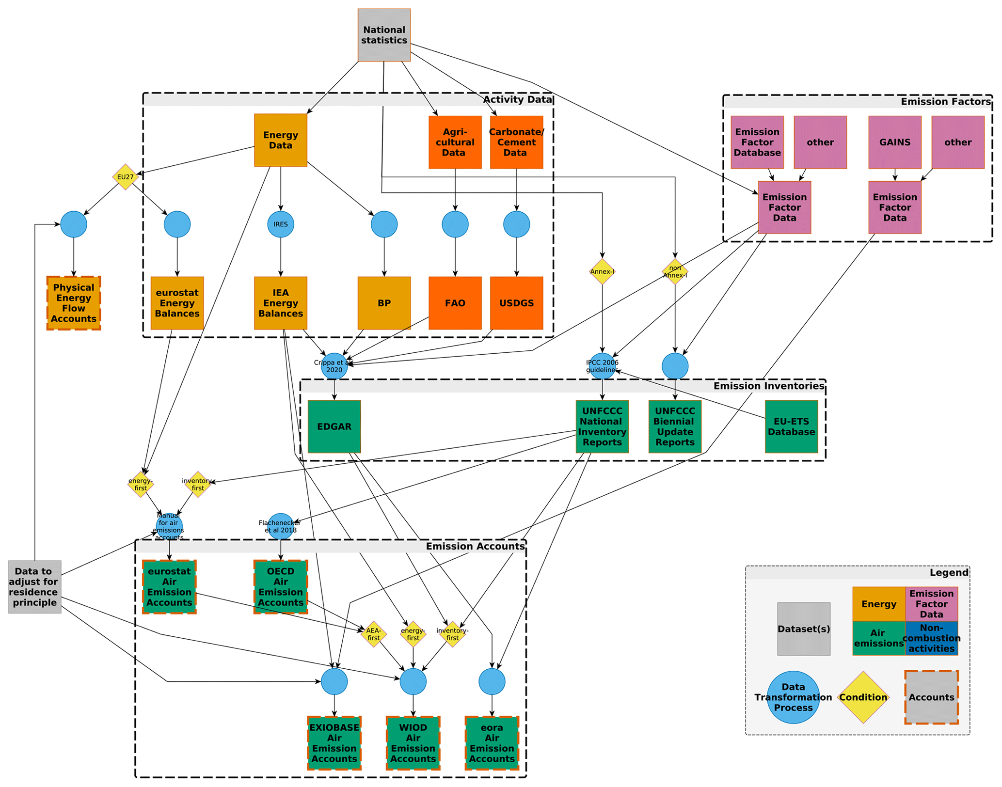
Figure A1Data sources used to compile selected GHG emission accounts. This is our own elaboration that builds on Andrew (2020) (emission data sets), Eurostat (2015) (Eurostat air emission accounts), Flachenecker et al. (2018) (OECD air emission accounts), Stadler et al. (2018) (EXIOBASE air emission accounts), Genty et al. (2012) (WIOD) and Lenzen et al. (2013, 2012) (Eora).
Since, to the best of our knowledge, there exists no proper framework to distinguish between different types of uncertainty in GMRIO analysis, we use the classification by Huijbregts (1998), who focuses on uncertainty and variability in the related discipline of life cycle assessment (LCA). Distinguishing variability from uncertainty, Huijbregts (1998) defines the former as “stemming from inherent variations in the real world”, while the latter is defined as coming “from inaccurate measurements, lack of data, model assumptions, etc.”. Variability, as defined by Huijbregts (1998), is sometimes also referred to as aleatoric uncertainty, while their understanding of uncertainty is often referred to as epistemic uncertainty (see e.g. Sullivan, 2015). Huijbregts (1998) further divide (epistemic) uncertainty into parameter uncertainty, model or scenario uncertainty and uncertainty due to choices as well as variability (aleatoric uncertainty) into spatial variability, temporal variability and variability between objects or sources (Table B1).
Table B1Different types of uncertainty and variability according to Huijbregts (1998). GMRIO examples are based on our own elaboration.
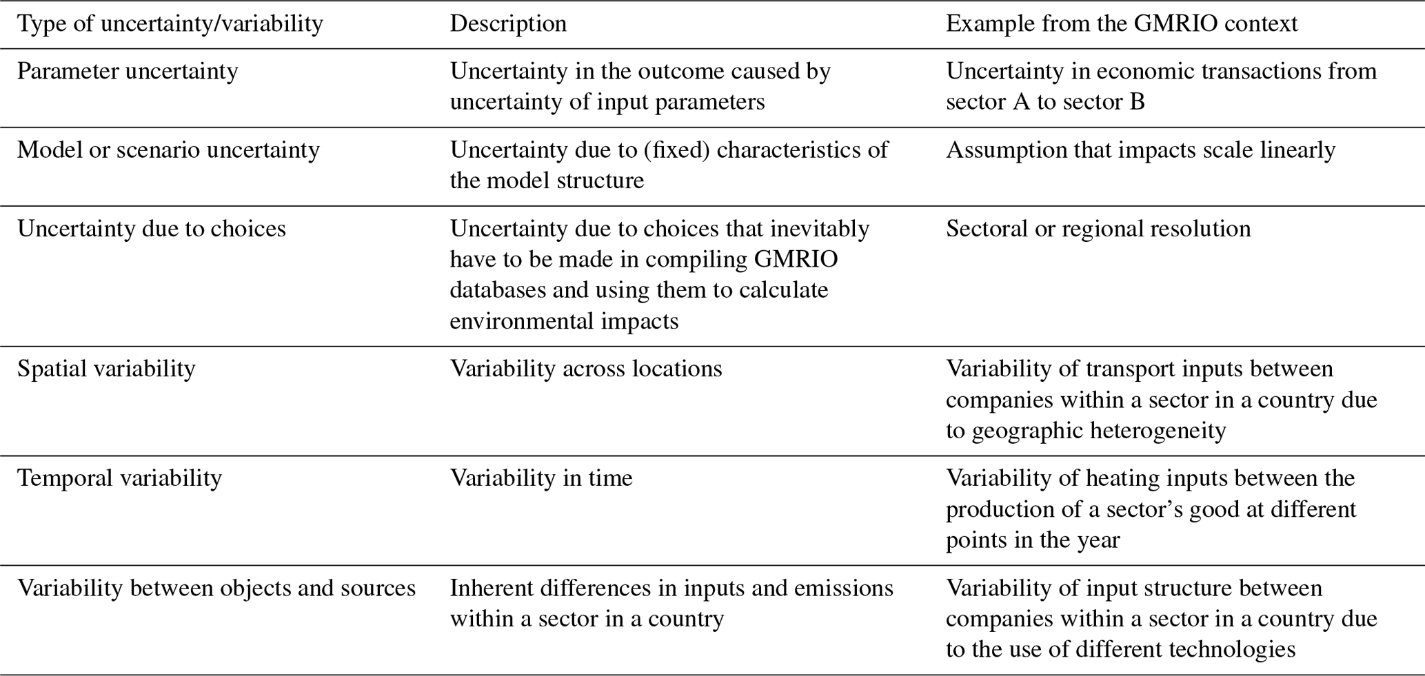
Table C1EXIOBASE V3 countries or regions and raw data sources (EDGAR or UNFCCC inventories). The column “Country code” shows ISO 3166-1 alpha-2 codes, except for the five Rest of the World (RoW) regions.
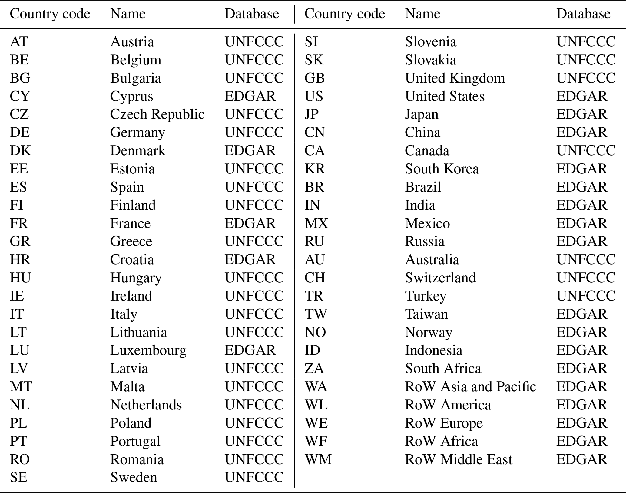
D1 International navigation and fishing
To estimate the bridging items for international water transport and fishing activities, we use data from Selin et al. (2021), who analysed the allocation of CO2 emissions from international shipping to national carbon budgets for the year 2015 using spatially resolved data on ship movements and ship-specific data on engine power demand, activity time and emission factor. The authors compared different allocation options: allocation based on flag country, owner country, operator country, manager country or bunker fuel country.
To be consistent with the SEEA, we use the allocation based on the operator country since the operator country is where the economic transactions related to the shipping activities are listed in the national accounts (as compared to the flag country, which is only responsible for ensuring that a ship meets all relevant legal standards).
To ensure consistency with global international shipping emissions from EDGAR, we do not directly take the bottom-up total emission estimates from Selin et al. (2021). Instead, we take the results from Selin et al. (2021) and calculate country-specific use shares by dividing individual countries' shipping CO2 emissions through the sum of all shipping CO2 emissions. Those use shares (which sum to 1) are multiplied by the total global international shipping emissions from EDGAR. Formally expressed, the emissions of GHG g from international shipping for country r are
where are all CO2 emissions caused by ships of which the operator is an institutional unit of country r and which serve international shipping or fishing purposes. are the global emissions related to international shipping from EDGAR.
Since Selin et al. (2021) only cover CO2 emissions, we use the CO2-related use shares for CH4 and N2O, too, thus making the implicit assumption that the ship-specific emission factors for CH4 and N2O are directly proportional to the CO2 emission factors.
D2 International air and road transport
Unfortunately, for international air and road transport, to the best of our knowledge, there exists no study of a similar scope and level of detail to the work of Selin et al. (2021) for international shipping. That is why, for both international air and road transport, we use the country-specific bridging items provided by Eurostat (Eurostat, 2022).
In the case of international road transport, we follow Stadler et al. (2018) and consider the EU countries to be by far the most affected by the residence adjustment of international road transport due to the European geography and its economic size (many countries in a relatively small area with a lot of cross-border commercial and recreational road transport). Non-European regions represented in EXIOBASE are “either islands or countries with limited road access in relation to their size (e.g. China, India)” (Stadler et al., 2018). Thus we assume that, for those countries, the road transport emissions from non-resident units operating on the country's national territory and the emissions from resident units operating abroad are the same. In other words, we assume the bridging items related to international road transport for non-EU countries to be 0. However, in contrast to international air and water transport, we have no knowledge about the total (global or European) emissions from international road transport, as they are not reported separately as memo items but as part of the road transport sector emissions (CRF category 1.A.3.b) within each country. That is why – instead of calculating use shares as we do for water transport – we directly take the total bridging items from Eurostat (Eurostat, 2022) and add or subtract those from the respective EU country's national road transport emissions.
In the case of international air transport, however, non-EU countries constitute a major, definitely non-negligible share of global international air transport emissions. Thus, we calculate country-specific use shares separately for EU countries (using Eurostat's bridging data) and non-EU countries. For the latter we use Worldbank data on the country-specific numbers of domestic and international air passengers carried by air carriers registered in the country as a proxy (Worldbank, 2023).
EU-country use shares we calculate as follows:
Non-EU-country use shares we calculate as follows:
D3 Special case: road transport
In the first step, we use Eurostat's PEFA data covering fuel-specific energy usage by NACE rev2 industries and households for all EU28 countries plus Iceland and Norway (Eurostat, 2023). We first calculate emissions from the use of “motor spirit” and “transport diesel” by industry sector or household s using the default fuel and GHG-specific emission factors from IPCC (2006):
where are the emissions from road transport using PEFA data and is the energy use from diesel or gasoline by both country r and sector s.
By summing emissions from both fuel types, we get total emissions by industry sector or household. To be consistent with UNFCCC and EDGAR inventories, we calculate industry- or household-specific use shares for each country,
and multiply those by the country-specific total emissions from road transport (1.A.3.b) from the UNFCCC and EDGAR:
Next, we allocate emissions from NACErev2 sectors to EXIOBASE sectors analogously using employment data as a proxy.
For countries not covered by Eurostat's PEFA (all non-EU countries except Norway and Iceland), we first split the country-specific total road transport emissions into household and industry emissions by using the weighted average household–industry split of all countries covered by PEFAs, with the total emissions from road transport as weights. We then further disaggregate the industry part using the employment data (see above).
In the case of countries not covered by Eurostat's PEFAs (all non-EU countries excluding Norway and Iceland), our approach involves initially splitting the total road transport emissions into household and industry emissions. To achieve this, we employ a weighted average household–industry split derived from all the countries covered by PEFAs, utilising the country-specific total emissions from road transport as the weighting factor. Subsequently, we proceed to disaggregate the industry portion by utilising employment data, as mentioned earlier.
E1 Fitting power law regressions to the raw data uncertainties
To examine how the “law of large numbers” which was used in the literature (Lenzen et al., 2010; Karstensen et al., 2015; Zhang et al., 2019) performs for the uncertainty data from UNFCCC and EDGAR, we fit power law regressions, both pooled and by country. The regressions have the form y=axb, where y is the CV and x is the size of an emission source (in terms of emissions).
From that exercise we see that, for CO2 and partly for CH4, there is a negative relation between the CV (coefficient of variation) and the size (in terms of emissions) of an emission source. This can be seen in the mostly negative slopes of the regression lines in Fig. E1a and the mostly negative values for the fitted parameters b (plot c). For N2O there is a large variability in the effect direction between the different countries with both negative and positive effects.
In general, R2s of the by-country regressions are larger for EDGAR than for the UNFCCC data. We assume that this results from the different level of aggregation of both data sources, which results in a larger variability in CVs for UNFCCC data due to their higher level of detail.
Furthermore, using pooled regression mostly delivers a worse fit (lower R2) than the by-country regressions. Moreover, we observe a large variability in the regression results between different countries, both in the direction of the relation between CV and size (plot c) and the R2 (plot b).
E2 Comparing our estimates to other databases
Figure E2 shows the comparison of the 95 % CIs of our GHG emission accounts with the estimates from EXIOBASE and the OECD.
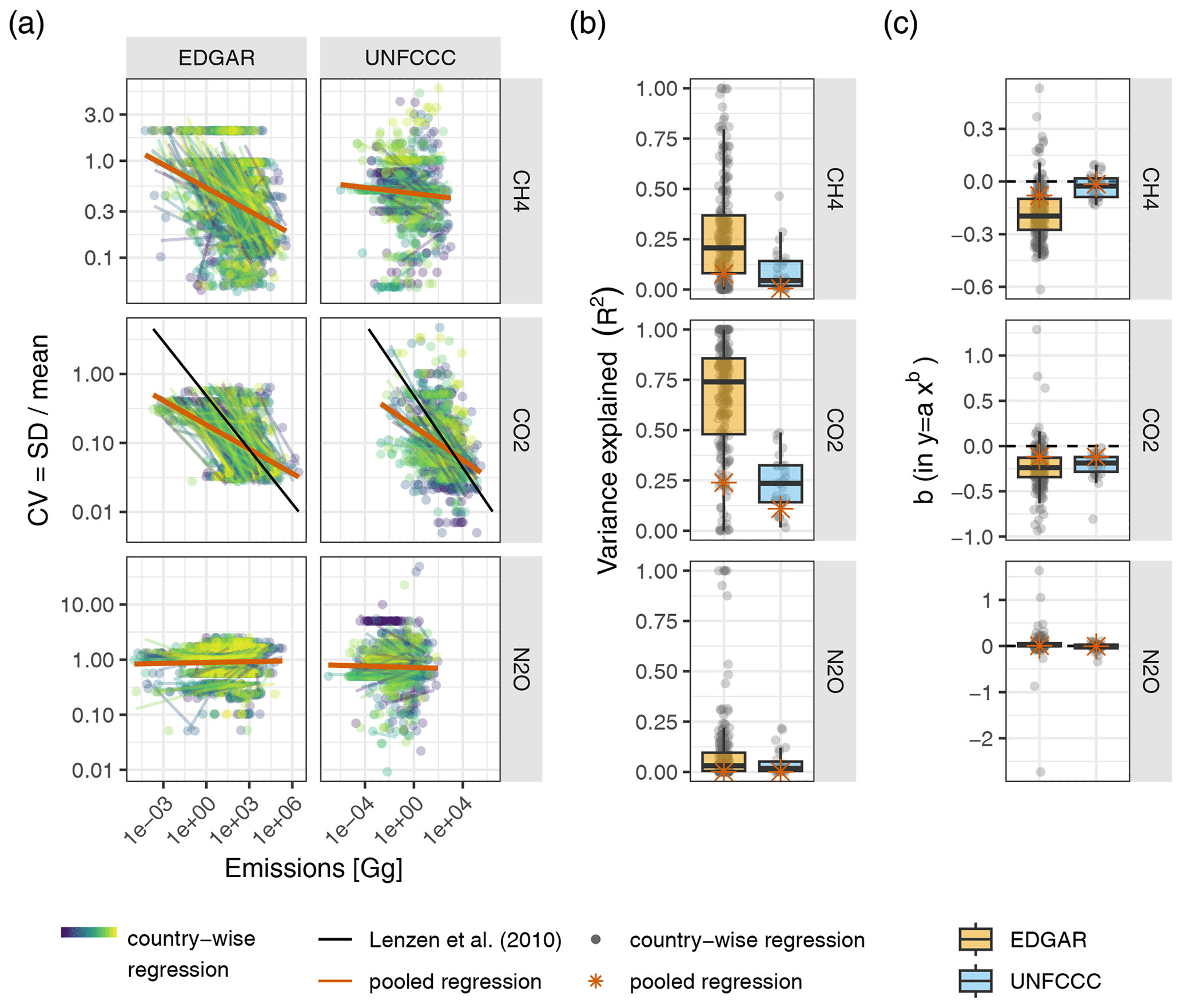
Figure E1Fitting power law regressions to the raw data uncertainties from the UNFCCC NIRs and EDGAR. The regressions have the form y=axb, where y is the CV and x is the size of an emission source (hence following Lenzen et al., 2010; Karstensen et al., 2015). The parameters a and b are fitted, either pooled (i.e. all data points together, red) or country-wise (i.e. a separate regression for each country, blue–green–yellow colour scale). (a) The data points along with the fitted regression lines. The black line shows the fit from Lenzen et al. (2010) (). (b) The distribution of the R2s of each of the regressions shown in panel (a). (c) The distribution of the fitted bs of each of the regressions shown in panel (a). A positive fitted b means a positive relation between CV and emission size and vice versa.
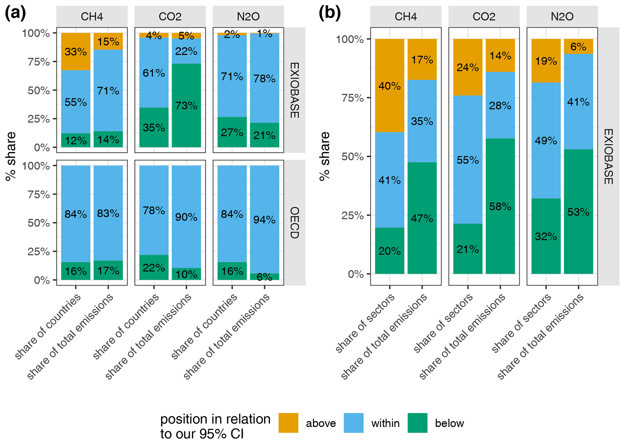
Figure E2Comparison of the 95 % CIs of our GHG emission accounts with the estimates from EXIOBASE and the OECD. (a) At the country level. (b) At the sector level. Comparison is made according to both the share of countries and sectors and the share of emissions those countries and sectors generate. Note that, due to the OECD's broad sector resolution, a direct comparison with our emission accounts at the sector level is not possible. In the case of comparison with the OECD estimate, 100 % refers to all countries and regions, which are covered in both our analysis and the OECD.
Table E1Industry sectors for which our sample means are considerably (i.e. for more than 75 % of all the regions) ABOVE the official EXIOBASE V3.8.2 estimate. Numerical values depict the median and 25 % and 75 % quantiles, respectively, of the sector-wise relative differences between our sample mean and the official EXIOBASE V3.8.2 estimate. A median of 19, for example, means that the median relative difference for that of a specific industry sector among all 49 regions is a factor of 19 compared to the official EXIOBASE estimates. CO2 only.
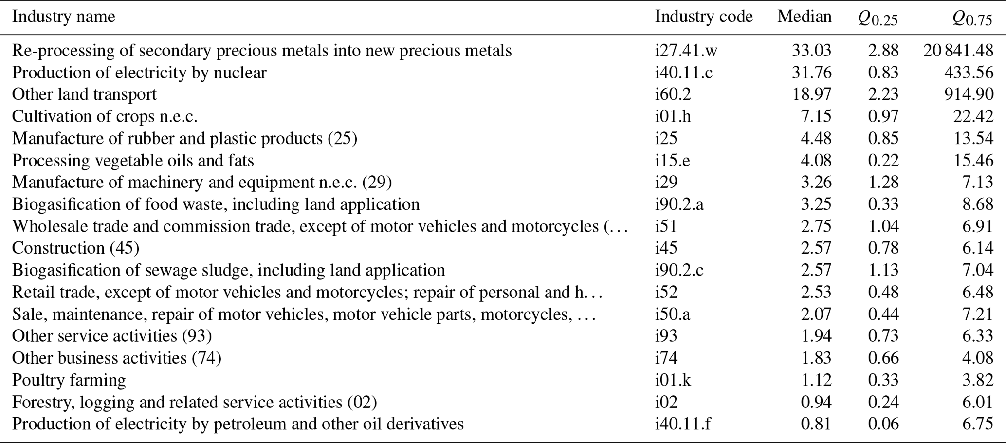
Table E2Industry sectors for which our sample means are considerably (i.e. for more than 75 % of all the regions) BELOW the official EXIOBASE V3.8.2 estimate. Numerical values depict the median and 25 % and 75 % quantiles, respectively, of the sector-wise relative differences between our sample mean and the official EXIOBASE V3.8.2 estimate. A median of −0.9, for example, means that the median relative difference for that of a specific industry sector among all 49 regions is a factor of −0.9 compared to the official EXIOBASE estimates. CO2 only.
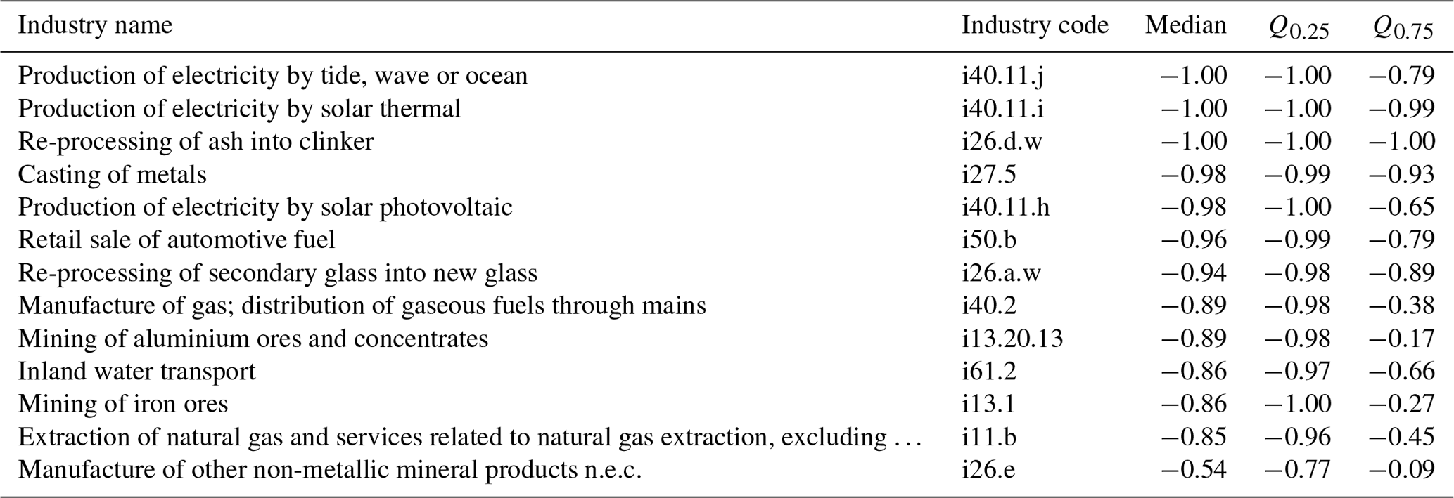
E3 Decomposing the uncertainty by source sector
Compiling GHG emission accounts from UNFCCC and EDGAR emission inventories involves allocating each emission source reported in the inventories to EXIOBASE target sectors and countries (see Sect. 2.1). Both UNFCCC and EDGAR report their emissions in CRF format.
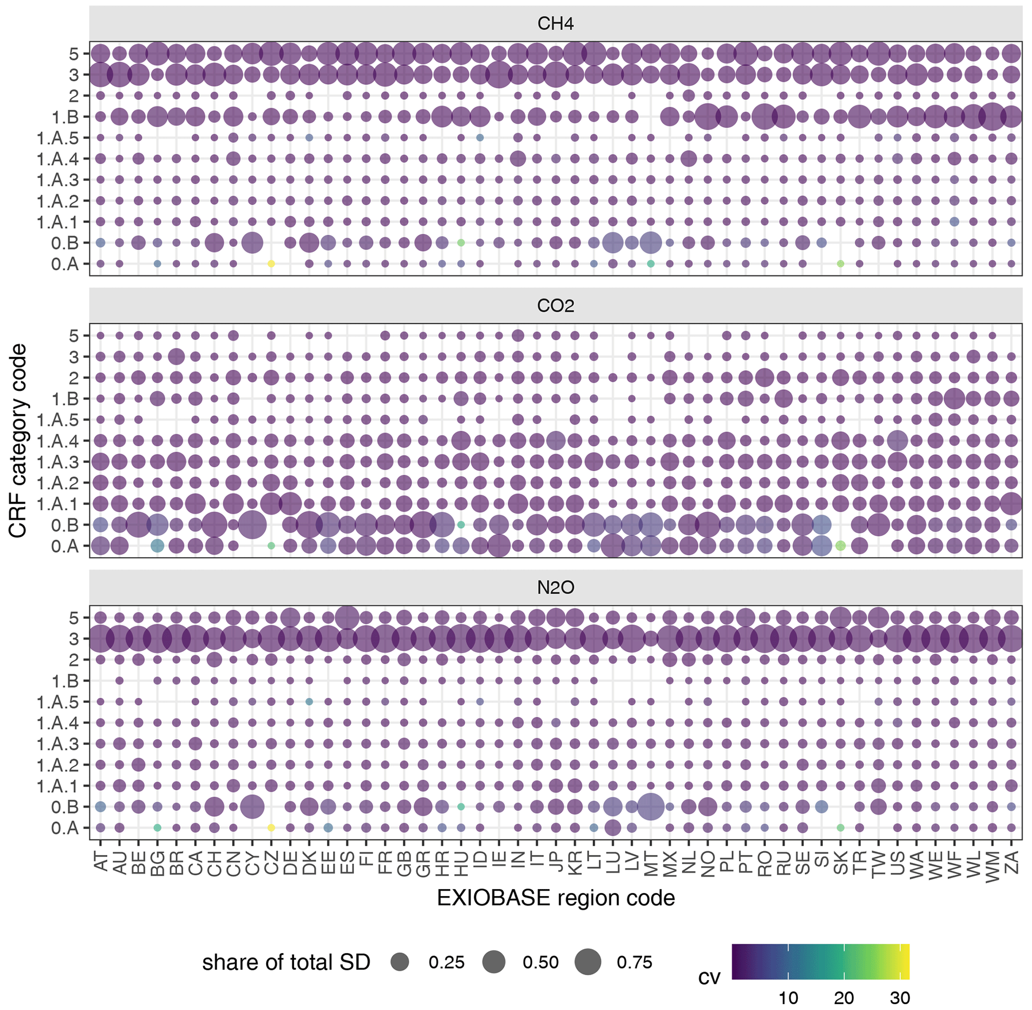
Figure E3Breakdown of the uncertainty by CRF category and country using bubble charts. The size of each bubble is adjusted according to the share of the standard deviation (SD) of the respective IPCC category in the sum of all SDs for each country.
Here, we aggregate all allocations by CRF category at a common level (depicting the emission source) and at the EXIOBASE region level (depicting the emission destination) to analyse which source categories contribute most to overall uncertainty by country. Figure E3 illustrates the absolute uncertainty by CRF category and country using bubble charts. The size of each bubble is adjusted according to the share of the standard deviation (SD) of the respective IPCC category in the sum of all SDs for each country. While interpreting the actual numbers, caution is advised since summing all SDs may not yield a meaningful calculation. Nevertheless, the visualisation remains helpful in identifying “hotspots” of uncertainty sources.
Regarding CO2 emissions, most countries exhibit the largest SD in the allocations of international air and water emissions. Additionally, road transportation (1.A.3) and other energy sources (1.A.4) also contribute significantly to the overall uncertainty in some countries. For CH4 emissions, the greatest uncertainty arises from agriculture (3) and waste (5), with varying compositions depending on each country. Fugitive emissions (1.B) are generally less pronounced but still constitute a major source in some countries. Notably, for a few countries like Malta, Cyprus, Denmark or Luxembourg, CH4 emissions from international water transport emerge as a significant source of uncertainty.
Concerning N2O emissions, emissions from agriculture (3) account for the largest uncertainty in almost all countries. However, for a few countries like Spain, Taiwan, Cyprus or Malta, emissions from waste treatment (5) and international shipping (0.B) also play a considerable role.
E4 Uncertainty at the sectoral level
Figure E4a, c and e show the uncertainty in GHG emission accounts next to the uncertainty of the GHG footprints (Fig. E4b, d and f). To allow comparison between the two, the measure of uncertainty is reduced to one number, the CV (y axis, orange line). Each coloured stripe represents one sector with the width and colour adjusted to the mean share in total emissions. In the case of GHG emission accounts, the mean share refers to the (total) production-based emissions of that sector, while in the case of the GHG footprints the mean share refers to the consumption-based emissions to satisfy the global final demand of that sector's product. The stripes are sorted along the x axis by their CV. The boxplots show the (unweighted) distributions of the CVs of the individual sectors.
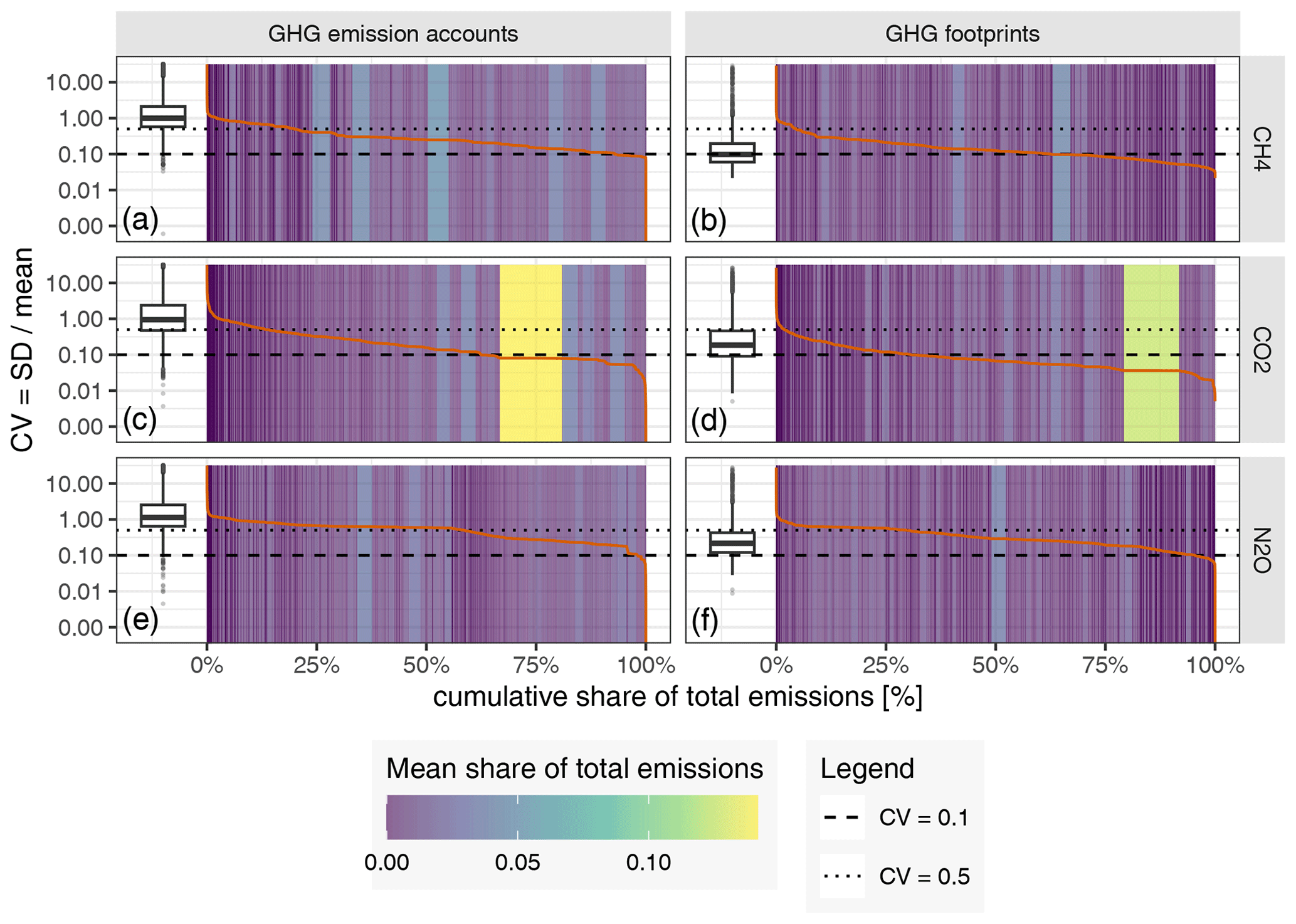
Figure E4The relative standard error (CVs) of the GHG emission accounts (a, c, e) and GHG footprints (b, d, f) at the sectoral level (coefficients) (orange line, y axis) by the cumulative share of the total emissions (x axis). Each coloured stripe represents one sector, with the width and colour adjusted to the mean share of the total emissions. The sectors are sorted along the x axis by their CV from high to low. The width and colour of the stripes are adjusted to the mean share of the total emissions. To ease interpretation, the dotted line marks a CV of 0.1 and the dashed line a CV of 0.5. The boxplots show the (unweighted) distributions of the CVs of the individual sectors.
Focusing on the uncertainty in GHG emission accounts (Fig. E4a, c and e), we see that the distributions of the CVs of the sectors look very similar between the three GHGs (Fig. E4 for boxplots, Table 2 for values). However, in the case of CO2, large uncertainties mostly occur with sectors with a relatively low share in total emissions, while sectors with relatively high CO2 emissions show in general a lower uncertainty. This can be seen in the distribution of the width and colours along the y axis in Fig. E4, where CO2 sectors with high emissions (large stretch along the x axis, yellow to green colour) are generally more situated towards the right (lower CV), while sectors with low CO2 emissions (small stretch along the x axis, blue colour to purple) are more present towards the left (high CV). For CH4 and N2O there is no clear trend between a sector's CV and its size in terms of emissions. Thus, high-emitting sectors (wide, yellow boxes) and low-emitting sectors (narrow, blue boxes) are much more evenly distributed along the y axis. This finding aligns well with what we saw in Fig. 7, i.e. that uncertainties in CH4 and N2O emissions are much more homogeneously distributed between sectors than in the case of CO2. We see that, for CO2, 37 % of all emissions stem from sectors with a CV of less than 0.1 (dashed line) and 85 % from sectors with a CV of less than 0.5 (dotted line), while for CH4 it is only 7 % (CV < 0.1) and 80 % (CV < 0.5) and for N2O only 2 % (CV < 0.1) and 41 % (CV < 0.5).
SiS, SP and AJ conceptualised and designed the research. SiS performed the computations and analysed the results. SiS, SP and AJ validated the results. SiS wrote the paper with inputs from all the authors.
The contact author has declared that none of the authors has any competing interests.
Publisher's note: Copernicus Publications remains neutral with regard to jurisdictional claims made in the text, published maps, institutional affiliations, or any other geographical representation in this paper. While Copernicus Publications makes every effort to include appropriate place names, the final responsibility lies with the authors.
We thank Joshua Heipel for helping with the extraction of the uncertainty data from the UNFCCC National Inventory Reports. Moreover, we thank two anonymous reviewers for their valuable comments.
This open-access publication was funded by the University of Freiburg.
This paper was edited by Kuishuang Feng and reviewed by two anonymous referees.
Abbood, K., Egilmez, G., and Meszaros, F.: Multi-region Input-Output-based Carbon and Energy Footprint Analysis of U.S. Manufacturing, Periodica Polytechnica Social and Management Sciences, 31, 91–99, https://doi.org/10.3311/PPso.19554, 2023. a, b, c
Andrew, R. M.: A comparison of estimates of global carbon dioxide emissions from fossil carbon sources, Earth Syst. Sci. Data, 12, 1437–1465, https://doi.org/10.5194/essd-12-1437-2020, 2020. a
Belgorodski, N., Greiner, M., Tolksdorf, K., and Schueller, K.: rriskDistributions: Fitting distributions to given data or known quantiles, manual, https://CRAN.R-project.org/package=rriskDistributions (last access: 22 December 2022), 2017. a
Ciroth, A., Muller, S., Weidema, B., and Lesage, P.: Empirically based uncertainty factors for the pedigree matrix in ecoinvent, Int. J. Life Cycle Ass., 21, 1338–1348, https://doi.org/10.1007/s11367-013-0670-5, 2016. a
Crippa, M., Guizzardi, D., Muntean, M., Olivier, J., Schaaf, E., Solazzo, E., Vignati, E., European Commission, and Joint Research Centre: Fossil CO2 emissions of all world countries: 2018 report, oCLC: 1111210409, http://dx.publications.europa.eu/10.2760/30158 (last access: 11 March 2021), 2018. a
Crippa, M., Guizzardi, D., Muntean, M., Schaaf, E., Solazzo, E., Monforti-Ferrario, F., Olivier, J., and Vignati, E.: Fossil CO2 emissions of all world countries – 2020 Report, Publications Office of the European Union, Luxembourg, https://doi.org/10.2760/143674, 2020a. a
Crippa, M., Solazzo, E., Huang, G., Guizzardi, D., Koffi, E., Muntean, M., Schieberle, C., Friedrich, R., and Janssens-Maenhout, G.: High resolution temporal profiles in the Emissions Database for Global Atmospheric Research, Scientific Data, 7, 121, https://doi.org/10.1038/s41597-020-0462-2, 2020b. a, b, c
EMEP and EEA: EMEP/EEA air pollutant emission inventory guidebook 2019, https://www.eea.europa.eu/publications/emep-eea-guidebook-2019 (last access: 22 April 2021), 2019. a
Eurostat: Manual for air emissions accounts: 2015 edition, Publications Office of the European Union, LU, https://ec.europa.eu/eurostat/web/products-manuals-and-guidelines/-/KS-GQ-15-009 (last access: 19 April 2021), https://doi.org/10.2785/527552, 2015. a, b, c, d, e, f, g, h
Eurostat: Air emissions accounts totals bridging to emission inventory totals [env_ac_aibrid_r2], https://ec.europa.eu/eurostat/web/products-datasets/-/env_ac_aibrid_r2 (last access: 1 September 2023), 2022. a, b, c, d
Eurostat: Energy supply and use by NACE Rev. 2 activity, https://ec.europa.eu/eurostat/web/products-datasets/-/env_ac_pefasu (last access: 16 November 2023), 2023. a, b, c
Flachenecker, F., Guidetti, E., and Pionnier, P.-A.: Towards global SEEA Air Emission Accounts: Description and evaluation of the OECD methodology to estimate SEEA Air Emission Accounts for CO2, CH4 and N2O in Annex-I countries to the UNFCCC, OECD Statistics Working Papers, No. 2018/11, OECD Publishing, Paris, https://doi.org/10.1787/7d88dfdd-en, 2018. a, b
Genty, A., Arto, I., and Neuwahl, F.: Final database of environmental satellite accounts: technical report on their compilation, WIOD deliverable, 4, https://dataverse.nl/api/access/datafile/199109 (last access: 19 April 2021), 2012. a
Groen, E. A. and Heijungs, R.: Ignoring correlation in uncertainty and sensitivity analysis in life cycle assessment: what is the risk?, Environ. Impact Asses., 62, 98–109, https://doi.org/10.1016/j.eiar.2016.10.006, 2017. a
Hertwich, E. G. and Wood, R.: The growing importance of scope 3 greenhouse gas emissions from industry, Environ. Res. Lett., 13, 104013, https://doi.org/10.1088/1748-9326/aae19a, 2018. a
Hong, C., Zhao, H., Qin, Y., Burney, J. A., Pongratz, J., Hartung, K., Liu, Y., Moore, F. C., Jackson, R. B., Zhang, Q., and Davis, S. J.: Land-use emissions embodied in international trade, Science, 376, 597–603, https://doi.org/10.1126/science.abj1572, 2022. a
Huijbregts, M. A. J.: Application of uncertainty and variability in LCA, Int. J. Life Cycle Ass., 3, 273, https://doi.org/10.1007/BF02979835, 1998. a, b, c, d, e, f, g, h, i
IPCC: 2006 IPCC guidelines for national greenhouse gas inventories, oCLC: 192005769, https://www.ipcc-nggip.iges.or.jp/public/2006gl/ (last access: 20 April 2021), 2006. a, b, c, d, e, f, g, h, i, j, k
IPCC: 2019 Refinement to the 2006 IPCC Guidelines for National Greenhouse Gas Inventories, http://119.78.100.173/C666//handle/2XK7JSWQ/270170 (last access: 29 November 2022), 2019. a, b
Jaynes, E. T.: Information Theory and Statistical Mechanics, Phys. Rev., 106, 620–630, https://doi.org/10.1103/PhysRev.106.620, 1957. a
Kanemoto, K., Shigetomi, Y., Hoang, N. T., Okuoka, K., and Moran, D.: Spatial variation in household consumption-based carbon emission inventories for 1200 Japanese cities, Environ. Res. Lett., 15, 114053, https://doi.org/10.1088/1748-9326/abc045, 2020. a, b, c
Karstensen, J., Peters, G. P., and Andrew, R. M.: Uncertainty in temperature response of current consumption-based emissions estimates, Earth Syst. Dynam., 6, 287–309, https://doi.org/10.5194/esd-6-287-2015, 2015. a, b, c, d, e, f, g
Ku, H. H.: Notes on the use of propagation of error formulas, J. Res. Nat. Bur. Stand., 70, 263–273, 1966. a, b
Lempert, R. J.: Shaping the Next One Hundred Years: New Methods for Quantitative, Long-Term Policy Analysis, Rand Corporation, tex.ids=lempert2003 googlebooksid: F2SzOwE0_bIC, 2003. a
Lenzen, M.: Aggregation Versus Disaggregation in Input–Output Analysis of the Environment, Econ. Syst. Res., 23, 73–89, https://doi.org/10.1080/09535314.2010.548793, 2011. a
Lenzen, M., Wood, R., and Wiedmann, T.: Uncertainty Analysis for Multi-Region Input–Output Models – a Case Study of the UK's Carbon Footprint, Econ. Syst. Res., 22, 43–63, https://doi.org/10.1080/09535311003661226, 2010. a, b, c, d, e, f, g, h, i, j, k, l, m
Lenzen, M., Kanemoto, K., Moran, D., and Geschke, A.: Mapping the Structure of the World Economy, Environ. Sci. Technol., 46, 8374–8381, https://doi.org/10.1021/es300171x, 2012. a
Lenzen, M., Moran, D., Kanemoto, K., and Geschke, A.: Building eora: a global multi-region input–output database at high country and sector resolution, Econ. Syst. Res., 25, 20–49, https://doi.org/10.1080/09535314.2013.769938, 2013. a, b, c, d, e, f, g, h
Lenzen, M., Geschke, A., West, J., Fry, J., Malik, A., Giljum, S., Milà i Canals, L., Piñero, P., Lutter, S., Wiedmann, T., Li, M., Sevenster, M., Potočnik, J., Teixeira, I., Van Voore, M., Nansai, K., and Schandl, H.: Implementing the material footprint to measure progress towards Sustainable Development Goals 8 and 12, Nat. Sustain., 5, 157–166, https://doi.org/10.1038/s41893-021-00811-6, 2022. a, b
Majeau-Bettez, G., Pauliuk, S., Wood, R., Bouman, E. A., and Strømman, A. H.: Balance issues in input–output analysis: A comment on physical inhomogeneity, aggregation bias, and coproduction, Ecol. Econ., 126, 188–197, https://doi.org/10.1016/j.ecolecon.2016.02.017, 2016. a
Miller, R. E. and Blair, P. D.: Input-output analysis: foundations and extensions, 2nd Edn., Cambridge University Press, ISBN 978-0-521-73902-3, 2009. a
Min, J. and Rao, N. D.: Estimating Uncertainty in Household Energy Footprints, J. Ind. Ecol., 22, 1307–1317, https://doi.org/10.1111/jiec.12670, 2018. a
Moran, D., Kanemoto, K., Jiborn, M., Wood, R., Többen, J., and Seto, K. C.: Carbon footprints of 13 cities, Environ. Res. Lett., 13, 064041, https://doi.org/10.1088/1748-9326/aac72a, 2018. a
Owen, A., Wood, R., Barrett, J., and Evans, A.: Explaining value chain differences in MRIO databases through structural path decomposition, Econ. Syst. Res., 28, 243–272, https://doi.org/10.1080/09535314.2015.1135309, 2016. a, b, c
Pan, C., Peters, G. P., Andrew, R. M., Korsbakken, J. I., Li, S., Zhou, D., and Zhou, P.: Emissions embodied in global trade have plateaued due to structural changes in China, Earths Future, 5, 934–946, https://doi.org/10.1002/2017EF000625, 2017. a
Paoli, L., Lupton, R. C., and Cullen, J. M.: Useful energy balance for the UK: An uncertainty analysis, Appl. Energ., 228, 176–188, https://doi.org/10.1016/j.apenergy.2018.06.063, 2018. a, b
Peters, G. P., Andrew, R., and Lennox, J.: Constructing an Environmentally-Extended Multi-Regional Input–Output Table Using the Gtap Database, Econ. Syst. Res., 23, 131–152, https://doi.org/10.1080/09535314.2011.563234, 2011. a
Pflüger, M. and Gütschow, J.: UNFCCC country-submitted greenhouse gas emissions data until 2020-10-25, Zenodo [data set], https://doi.org/10.5281/zenodo.4199622, 2020. a
Plessis, S., Carrasco, N., and Pernot, P.: Knowledge-based probabilistic representations of branching ratios in chemical networks: The case of dissociative recombinations, J. Chem. Phys., 133, 134110, https://doi.org/10.1063/1.3479907, 2010. a, b, c
Pulles, T., van het Bolscher, M., Brand, R., and Visschedijk, A.: Assessment of global emissions from fuel combustion in the final decades of the 20th Century, TNO Rep. 2007-A-R0132B, 2007. a
Pulles, T., Gillenwater, M., and Radunsky, K.: CO2 emissions from biomass combustion Accounting of CO2 emissions from biomass under the UNFCCC, Carbon Manag., 13, 181–189, https://doi.org/10.1080/17583004.2022.2067456, 2022. a
Reale, F., Cinelli, M., and Sala, S.: Towards a research agenda for the use of LCA in the impact assessment of policies, Int. J. Life Cycle Ass., 22, 1477–1481, https://doi.org/10.1007/s11367-017-1320-0, 2017. a
Rodrigues, J., Marques, A., Wood, R., and Tukker, A.: A network approach for assembling and linking input–output models, Econ. Syst. Res., 28, 518–538, https://doi.org/10.1080/09535314.2016.1238817, 2016. a
Rodrigues, J. D. F.: Maximum-Entropy Prior Uncertainty and Correlation of Statistical Economic Data, J. Bus. Econ. Stat., 34, 357–367, https://doi.org/10.1080/07350015.2015.1038545, 2016. a, b, c
Rodrigues, J. F. D.: A Bayesian Approach to the Balancing of Statistical Economic Data, Entropy, 16, 1243–1271, https://doi.org/10.3390/e16031243, 2014. a
Schulte, S.: Correspondence table between UNFCCC CRF and EXIOBASE industry sectors, Zenodo [data set], https://doi.org/10.5281/zenodo.10046372, 2023a. a, b
Schulte, S.: simschul/uncertainty_GHG_accounts: Submission 1 (v0.1.0), Zenodo [code], https://doi.org/10.5281/zenodo.10141616, 2023b. a
Schulte, S. and Heipel, J.: Uncertainties from the UNFCCC national inventory reports (submission 2017), Zenodo [data set], https://doi.org/10.5281/zenodo.10037714, 2023. a, b
Schulte, S., Jakobs, A., and Pauliuk, S.: Relaxing the import proportionality assumption in multi-regional input–output modelling, J. Econ. Struct., 10, 20, https://doi.org/10.1186/s40008-021-00250-8, 2021. a
Schulte, S., Pauliuk, S., and Jakobs, A.: Uncertainty of EXIOBASE GHG emission acounts 2015, Zenodo [data set], https://doi.org/10.5281/zenodo.10041196, 2023. a, b, c
Schulte, S., Jakobs, A., and Pauliuk, S.: Divide and rule: A practical overview of uncertainty propagation in the case of data disaggregation, in preparation, 2024. a, b
Selin, H., Zhang, Y., Dunn, R., Selin, N. E., and Lau, A. K. H.: Mitigation of CO2 emissions from international shipping through national allocation, Environ. Res. Lett., 16, 045009, https://doi.org/10.1088/1748-9326/abec02, 2021. a, b, c, d, e, f, g
Shrestha, P. and Sun, C.: Carbon Emission Flow and Transfer through International Trade of Forest Products, Forest Sci., 65, 439–451, https://doi.org/10.1093/forsci/fxz003, 2019. a, b, c
Solazzo, E., Crippa, M., Guizzardi, D., Muntean, M., Choulga, M., and Janssens-Maenhout, G.: Uncertainties in the Emissions Database for Global Atmospheric Research (EDGAR) emission inventory of greenhouse gases, Atmos. Chem. Phys., 21, 5655–5683, https://doi.org/10.5194/acp-21-5655-2021, 2021. a, b, c, d, e, f, g, h, i, j, k, l, m, n
Stadler, K., Wood, R., Bulavskaya, T., Södersten, C.-J., Simas, M., Schmidt, S., Usubiaga, A., Acosta-Fernández, J., Kuenen, J., Bruckner, M., Giljum, S., Lutter, S., Merciai, S., Schmidt, J. H., Theurl, M. C., Plutzar, C., Kastner, T., Eisenmenger, N., Erb, K.-H., Koning, A. d., and Tukker, A.: EXIOBASE 3: Developing a Time Series of Detailed Environmentally Extended Multi-Regional Input-Output Tables, J. Ind. Ecol., 22, 502–515, https://doi.org/10.1111/jiec.12715, 2018. a, b, c, d, e, f, g, h, i, j, k, l
Stadler, K., Wood, R., Bulavskaya, T., Södersten, C.-J., Simas, M., Schmidt, S., Usubiaga, A., Acosta-Fernández, J., Kuenen, J., Bruckner, M., Giljum, S., Lutter, S., Merciai, S., Schmidt, J. H., Theurl, M. C., Plutzar, C., Kastner, T., Eisenmenger, N., Erb, K.-H., Koning, A., and Tukker, A.: Exiobase 3, Zenodo [data set], https://doi.org/10.5281/zenodo.5589597, 2021. a, b, c
Steininger, K. W., Lininger, C., Meyer, L. H., Muñoz, P., and Schinko, T.: Multiple carbon accounting to support just and effective climate policies, Nat. Clim. Change, 6, 35–41, https://doi.org/10.1038/nclimate2867, 2016. a
Sullivan, T.: Introduction to Uncertainty Quantification, vol. 63 of Texts in Applied Mathematics, Springer International Publishing, Cham, https://doi.org/10.1007/978-3-319-23395-6, 2015. a
Tukker, A., Koning, A. D., Owen, A., Lutter, S., Bruckner, M., Giljum, S., Stadler, K., Wood, R., and Hoekstra, R.: Towards Robust, Authoritative Assessments of Environmental Impacts Embodied in Trade: Current State and Recommendations, J. Ind. Ecol., 22, 585–598, https://doi.org/10.1111/jiec.12716, 2018. a, b, c, d, e, f, g
Tukker, A., Pollitt, H., and Henkemans, M.: Consumption-based carbon accounting: sense and sensibility, Clim. Policy, 20, S1–S13, https://doi.org/10.1080/14693062.2020.1728208, 2020. a, b
UN, FAO, OECD, EU, IMF, and WB: System of Environmental-Economic Accounting 2012: Central Framework, White cover publication, ISBN 987-92-1-161563-0 2014. a, b
Usubiaga, A. and Acosta-Fernández, J.: Carbon Emission Accounting in Mrio Models: The Territory Vs. the Residence Principle, Econ. Syst. Res., 27, 458–477, https://doi.org/10.1080/09535314.2015.1049126, 2015. a
Wiebe, K. S. and Lenzen, M.: To RAS or not to RAS? What is the difference in outcomes in multi-regional input–output models?, Econ. Syst. Res., 28, 383–402, 2016. a
Wiebe, K. S. and Yamano, N.: Estimating CO2 Emissions Embodied in Final Demand and Trade Using the OECD ICIO 2015: Methodology and Results, Tech. rep., OECD, Paris, https://doi.org/10.1787/5jlrcm216xkl-en, 2016. a
Wilting, H. C.: Sensitivity and Uncertainty Analysis in Mrio Modelling; Some Empirical Results with Regard to the Dutch Carbon Footprint, Econ. Syst. Res., 24, 141–171, https://doi.org/10.1080/09535314.2011.628302, 2012. a, b, c, d
Worldbank: Air transport, passengers carried – Data, https://data.worldbank.org/indicator/IS.AIR.PSGR (last access: 4 January 2023), 2023. a, b
Zhang, H., He, K., Wang, X., and Hertwich, E. G.: Tracing the Uncertain Chinese Mercury Footprint within the Global Supply Chain Using a Stochastic, Nested Input–Output Model, Environ. Sci. Technol., 53, 6814–6823, https://doi.org/10.1021/acs.est.8b06373, 2019. a, b, c, d, e, f
Germany was chosen for two reasons. First, it is a major GHG-emitting country, and second, with ± 1000 pages the German NIR is one of the most detailed reports of all the submitting countries.
- Abstract
- Introduction
- Material and methods
- Results
- Discussion
- Code and data availability
- Conclusions
- Appendix A: Comparing the GHG emission account compilation between different databases
- Appendix B: Sources of uncertainty in GMRIO
- Appendix C: EXIOBASE regions
- Appendix D: Methods
- Appendix E: Additional results
- Author contributions
- Competing interests
- Disclaimer
- Acknowledgements
- Financial support
- Review statement
- References