Greenhouse gas emissions and their trends over the last 3 decades across Africa

A key goal of the Paris Agreement (PA) is to reach net-zero greenhouse gas (GHG) emissions by 2050 globally, which requires mitigation efforts from all countries. Africa's rapidly growing population and gross domestic product (GDP) make this continent important for GHG emission trends. In this paper, we study the emissions of carbon dioxide (CO₂), methane (CH₄) and nitrous oxide (N₂O) in Africa over 3 decades (1990–2018). We compare bottom-up (BU) approaches, including United Nations Convention Framework on Climate Change (UNFCCC) national inventories, FAO, PRIMAP-hist, process-based ecosystem models for CO₂ fluxes in the land use, land use change and forestry (LULUCF) sector and global atmospheric inversions. For inversions, we applied different methods to separate anthropogenic CH₄ emissions. The BU inventories show that, over the decade 2010–2018, fewer than 10 countries represented more than 75 % of African fossil CO₂ emissions. With a mean of 1373 Mt CO₂ yr⁻¹, total African fossil CO₂ emissions over 2010–2018 represent only 4 % of global fossil emissions. However, these emissions grew by +34 % from 1990–1999 to 2000–2009 and by +31 % from 2000–2009 to 2010–2018, which represents more than a doubling in 30 years. This growth rate is more than 2 times faster than the global growth rate of fossil CO₂ emissions. The anthropogenic emissions of CH₄ grew by 5 % from 1990–1999 to 2000–2009 and by 14.8 % from 2000–2009 to 2010–2018. The N₂O emissions grew by 19.5 % from 1990–1999 to 2000–2009 and by 20.8 % from 2000–2009 to 2010–2018. When using the mean of the estimates from UNFCCC reports (including the land use sector) with corrections from outliers, Africa was a mean source of greenhouse gases of ${\mathrm{2622}}_{\mathrm{2186}}^{\mathrm{3239}}$ Mt CO₂ eq. yr⁻¹ from all BU estimates (the subscript and superscript indicate min–max range uncertainties) and of $+{\mathrm{2637}}_{\mathrm{1761}}^{\mathrm{5873}}$ Mt CO₂ eq. yr⁻¹ from top-down (TD) methods during their overlap period from 2001 to 2017. Although the mean values are consistent, the range of TD estimates is larger than the one of the BU estimates, indicating that sparse atmospheric observations and transport model errors do not allow us to use inversions to reduce the uncertainty in BU estimates. The main source of uncertainty comes from CO₂ fluxes in the LULUCF sector, for which the spread across inversions is larger than 50 %, especially in central Africa. Moreover, estimates from national UNFCCC communications differ widely depending on whether the large sinks in a few countries are corrected to more plausible values using more recent national sources following the methodology of Grassi et al. (2022). The medians of CH₄ emissions from inversions based on satellite retrievals and surface station networks are consistent with each other within 2 % at the continental scale. The inversion ensemble also provides consistent estimates of anthropogenic CH₄ emissions with BU inventories such as PRIMAP-hist. For N₂O, inversions systematically show higher emissions than inventories, on average about 4.5 times more than PRIMAP-hist, either because natural N₂O sources cannot be separated accurately from anthropogenic ones in inversions or because BU estimates ignore indirect emissions and underestimate emission factors. Future improvements can be expected thanks to a denser network of monitoring atmospheric concentrations. This study helps to introduce methods to enhance the scope of use of various published datasets and allows us to compute budgets thanks to recombinations of those data products. Our results allow us to understand uncertainty and trends in emissions and removals in a region of the world where few observations exist and where most inventories are based on default IPCC guideline values. The results can therefore serve as a support tool for the Global Stocktake (GST) of the Paris Agreement. The referenced datasets related to the figures are available at https://doi.org/10.5281/zenodo.7347077 (Mostefaoui et al., 2022).

1 Introduction

Large global reductions in greenhouse gas (GHG) emissions are needed to avoid “dangerous anthropogenic interference with the climate system” (IPCC, 2021). The Paris Agreement (PA) aims at limiting global warming below 2 ^∘C and reaching net-zero GHG emissions by 2050. To improve the monitoring of emission trends, the PA has an Enhanced Transparency Framework (ETF) by which countries will have to report their GHG emissions and removals under a standardized format starting in 2024 (Perugini et al., 2021; UNFCCC, 2021) through Biennial Transparency Reports (BTRs), with the aim of using up-to-date data and best-available science to improve national inventories. This represents a challenge for many developing countries, where emission inventories have been irregular.

Recent analyses predict a fast increase in African emissions correlated with demographic growth. The African population is expected to double from 1.2 billion in 2019 to 2.5 billion at the 2050 horizon (UN, 2019). Using the TIAM-ECN Integrated Assessment Model (IAM) developed with data from the International Energy Agency (IEA), van der Zwaan et al. (2018) concluded that GHG emissions from Africa will become substantial at the global scale by 2050. In shared socioeconomic pathway (SSP) projection scenarios, Africa and the Middle East are grouped together despite having very different geographies, per capita emissions and gross domestic products (GDPs) (IIASA, 2017). According to IAM projections, the minimum projected share of Africa in global emissions would be close to 10 % by 2050 for a business-as-usual pathway. An “explosive growth in African combustion emissions”' (Liousse et al., 2014) could not be excluded from 2030 to 2050 if no drastic mitigation policies are implemented (IPCC, 2021). If a stringent emission reduction pathway limiting global warming to +2 ^∘C is adopted, Africa could contribute around 20 % of global emissions by 2050, becoming the second largest worldwide emitting region. Further, under stringent climate policy scenarios, CH₄ and N₂O emissions in Africa were projected to contribute 80 % of the total emissions of these two gases in 2050 (van der Zwaan et al., 2018). Therefore, Africa will become an important global emission contributor under any mitigation pathway with a demographic and industrial development increase.

There are 56 African countries represented in the United Nations. National emission reports to the United Nations Convention Framework on Climate Change (UNFCCC) are available for 53 countries, including all major African emitters. Africa as a whole ranks fifth worldwide in terms of territorial fossil fuel use with a total of 1449 Mt CO₂ eq., in between the Russian Federation and Japan (Friedlingstein et al., 2020). The global share of Africa is ∼4 % of fossil CO₂ (FCO₂) emissions, ∼16 % of CH₄ emissions (Saunois et al., 2020) and ∼25 % of N₂O emissions (Tian et al., 2020). South Africa is the biggest FCO₂ emitter on the continent and ranks twelfth on the global scale, just after Brazil.

Despite projections of strong growth of emissions and population in Africa, the continent is understudied and lacks up-to-date comprehensive assessments of GHG emissions and removals, given sporadic and often outdated reports by individual countries. The literature tends to be scarce on African countries, and their emissions have rarely been analyzed comprehensively using the results from both statistical inventories that are also referred to as bottom-up (BU) methods and top-down (TD) atmospheric inversions. Country reports estimate GHG emissions through statistical inventories using estimates of national sectoral activity data multiplied by emission factors, with three levels of refinements depending on countries, named Tier 1 for default emission factors, Tier 2 for country-specific emission factors or activity data and Tier 3 for more emission factors or activity with tailored representation at the scale of the process. Other BU inventories for assessing national emissions also exist: they are based on the same approach as country-reported inventories but use their own parameters for activity data and emission factors coming from research groups, international statistical agencies, etc. Process-based ecosystem models developed by the research community are not used by countries. They are based on the representations of complex ecosystem processes and can also be viewed as a BU method. In addition, another approach is named “top-down” and refers to atmospheric inversions. Inversions consist in estimating causes (emissions and sinks) based on consequences (concentrations). The inverse modeling approach consists in adjusting a priori fluxes to the atmospheric transport in order to be as adjusted as possible with observation data by minimizing a cost function. This is a mathematically complex problem under-constrained because every point of the globe is an unknown emission, and there are only a limited number of observations: “regularization” techniques are used to find a unique solution. The African ground-based atmospheric network used by inversions is very sparse. There are only three currently active surface flasks over this whole continent, located in Namibia (Gobabeb), in the Seychelles (Mahé) and in South Africa (Cape Point). The one in Algeria (Assekrem) was terminated on 26 August 2020, and the one in Kenya has been inactive since 21 June 2011. The characteristics of the surface flasks in Africa available on the NOAA website are summarized in Table S1 in the Supplement. Inversion results are therefore uncertain due to this small number of atmospheric stations over the continent (Nickless et al., 2020).

A previous analysis of African emissions was solely focused on FCO₂ emissions during the decade 2000–2009 (Canadell et al., 2009). A first budget for the period 1990–2009 was provided at the continental scale with the RECCAP1 project (Valentini et al., 2014). Ayompe et al. (2020) studied recent FCO₂ emission trends using IEA data. Other studies are region-specific or sector-specific, focusing exclusively on agriculture (Bombelli et al., 2009), on natural ecosystems in sub-Saharan Africa (Kim et al., 2016) or on individual countries such as Kenya (Zhu et al., 2018).

Paying attention not only to commonly identified big emitters like South Africa but also to medium emitters and emerging emitters is important, not only in terms of scientific assessment but also for financial and climate policy purposes under the PA. The monitoring, reporting and verification (MRV) provisions of the PA indeed require scientific and policy tools to verify the pledges made by all the signatory countries. Instruments for financial transfers for mitigation and adaptation like the Green Fund on Climate Change (GCF) and the REDD+ initiatives cover the African scope and will require scientific assessment of trends for impact evaluation and credibility purposes and as an incentive for continued investments. As part of the Global Stocktake (GST) under article 14 of the PA aiming at assessing “collective progress”, all the signatory parties will have to show their contributions to global mitigation efforts. These efforts will be evaluated within an MRV system which includes the requirement for developing countries to submit their Biennial Update Reports (BURs) on a biennial basis starting in 2024. As no standard global reporting framework has been required to date, we anticipate that the data available for the first stocktake in 2023 will be very heterogeneous. As a continent that includes non-Annex I countries exclusively, the African case is characterized by the scarcity of national official inventories, which have been provided to date on a voluntary basis through the National Communication (NC) and BURs. BU estimates of emissions established by independent scientific methods are also discussed in the present study. In this context, different and complementary observation-based methods assessing national GHG emissions and sinks are needed.

The aim of this paper is to evaluate the relative merits of different existing types of datasets for the assessment of African emissions and removals and their trends for CO₂, CH₄ and N₂O during the last 3 decades. In this paper, we standardize the metrics and the scope of application for different categories of GHG emissions to discuss budgets. We also validate and benchmark different independent datasets to evaluate the possibility of using them as a verifying tool for official country-reported data. In order to cover all the GHG sectors, we also describe recombinations of different historical datasets for the last 30 years that are necessary for filling the gap for some missing past sectoral emissions. This study offers a comparison of data products originally combined to compute a budget and an evaluation of their relative merits. The different data products discussed here include different BU approaches, including official country communications to the UNFCCC and estimations from the Food and Agriculture Organization (FAO), the Carbon Dioxide Information Analysis Center (CDIAC), global inventories for anthropogenic emissions (PRIMAP-hist, which integrates combinations of various datasets including FAO and the Global Carbon Project GCP) and process-based models for land CO₂ fluxes with 14 dynamic general vegetation models (DGVMs) from the TRENDY version 9 ensemble (Table 1). We also analyze and combine TD products to discuss individual gases and to compute budgets: 3 atmospheric global inversions for CO₂ land fluxes, 22 inversions for CH₄ emissions (11 inversion models using surface station data and 11 satellite inversion models) and CH₄ wildfire emissions from the Global Fires Emission Dataset (GFED) version 4. We used three inversion models for N₂O fluxes (the PyVAR model, TOMCAT-INVICAT model and MIROC4-ACTM model; see Table 1). Inversions only solve for total fluxes or at best for groups of sectors, whereas BU estimates have a larger number of sectors. In Table 2, we present the correspondence between “sectors” defined by the TD and BU methods. For all the datasets, we chose an atmospheric convention with negative values representing removals from the atmosphere (i.e., a land sink). We deliver an original comparison of BU estimates from national inventories, global inventories and process-based models, with TD estimates from atmospheric inversions over Africa. The work is carried out for large countries or groups of small countries, as inversions do not have the capability to constrain fluxes over small areas given their coarse grid and sparse atmospheric data. Based on the benchmarking and relative merit evaluation of the various data products presented above, the scientific questions addressed in this study are the following. (1) How consistent are the mean values and trends of GHG emissions across BU estimates in Africa? (2) How consistent are the different inversion model results? (3) How do inversions compare with BU estimates? (4) What is the net GHG balance of the African continent from different observation-based methods, including CO₂ sinks and sources in the land use sector? (5) What are the main sources of uncertainties?

The paper is organized into two main sections. First, a material and methods section describes the regional breakdown and input data (Sect. 1). We present our results for the whole of Africa and for six groups of aggregated countries (Sect. 2) with a specific analysis of CO₂ emissions and sinks, divided between FCO₂ (Sect. 2.1), fluxes in the land use, land use change and forestry (LULUCF) sector (Sect. 2.2) and emissions of non-CO₂ greenhouse gases (Sect. 2.3 and 2.4). Conclusions are drawn about uncertainties in African GHG net emissions and removal assessment.

2 Methods, datasets and dataset usage

This study covers the period from 1990 to 2018 as well as emissions and sinks of CO₂, CH₄ and N₂O. We used 1990 as a base year since reporting to the UNFCCC mostly started in that year and is often used as a reference comparison year in national pledges of the PA. The last year of analysis is 2018, reflecting the availability of inversion data and avoiding further uncertainty due to poorly understood emission changes before and after the COVID-19 crisis. This period allows the analysis of decadal features. It also has the advantage of being covered by several datasets listed in Table 1. We considered different BU approaches, including official country communications to the UNFCCC and estimations from the FAO, global inventories for anthropogenic emissions (PRIMAP-hist, which integrates combinations of various datasets, including FAO, GCP, EDGAR v4.3.2, Andrew 2018 cement data, BURs, Common Reporting Format (CRF), UNFCCC data, and BP) and process-based models for land CO₂ fluxes with 14 DGVMs from the TRENDY version 9 ensemble (Table 1). We used three atmospheric global inversions for CO₂ land fluxes, 22 inversions for CH₄ emissions and three inversions for N₂O fluxes (Table 1). For preliminary data quality control, we checked the consistency of prior fluxes by plotting them separately (Fig. S1 in the Supplement). Inversions only solve for total fluxes or at best for groups of sectors, whereas BU estimates have a larger number of sectors. In Table 2, we present the correspondence between the “sectors” defined by the TD and BU methods. For all the datasets, we chose an atmospheric convention with negative values representing removals from the atmosphere (i.e., the land sink). No specific standard guidelines currently exist to define uncertainties in the BU and TD data products. Given that some of our estimates are based on a small number of models and estimates, we cannot calculate the full distribution, e.g., with a 95 % confidence interval, but we rather reported ranges with minima and maxima. Assuming that the unknown distributions are Gaussian, like in Schulze et al. (2018), we could infer a 2σ (≈95 %) confidence interval if we assume that the minima and maxima are equivalent to 3σ, but in view of the small numbers of estimates, e.g., for N₂O with only three inversions, we prefer to just give the min–max range. Moreover, for national inventories, as all African countries are non-Annex I, they do not deliver confidence intervals, but Grassi et al. (2022) estimated for CO₂ LULUCF flux uncertainties of 50 % for the average of non-Annex-1 countries. Here, uncertainty estimates are understood as the spread among minimum and maximum values from one methodology. The main source of uncertainty in the comparison of country-reported data with other data products is the inclusion or not of natural fluxes in addition to anthropogenic emission sectors. For the comparability of the different data products presented in this study, we only discuss the mean value over the period of overlapping data availability. The referenced datasets are available at https://doi.org/10.5281/zenodo.7347077 (Mostefaoui et al., 2022).

Table 1 List of the BU and TD methods used. For more details, see also Saunois et al. (2020) for CH₄, Friedlingstein et al. (2020) for FCO₂, UNFCCC country-reported data and Gütschow et al. (2021) for PRIMAP-hist.

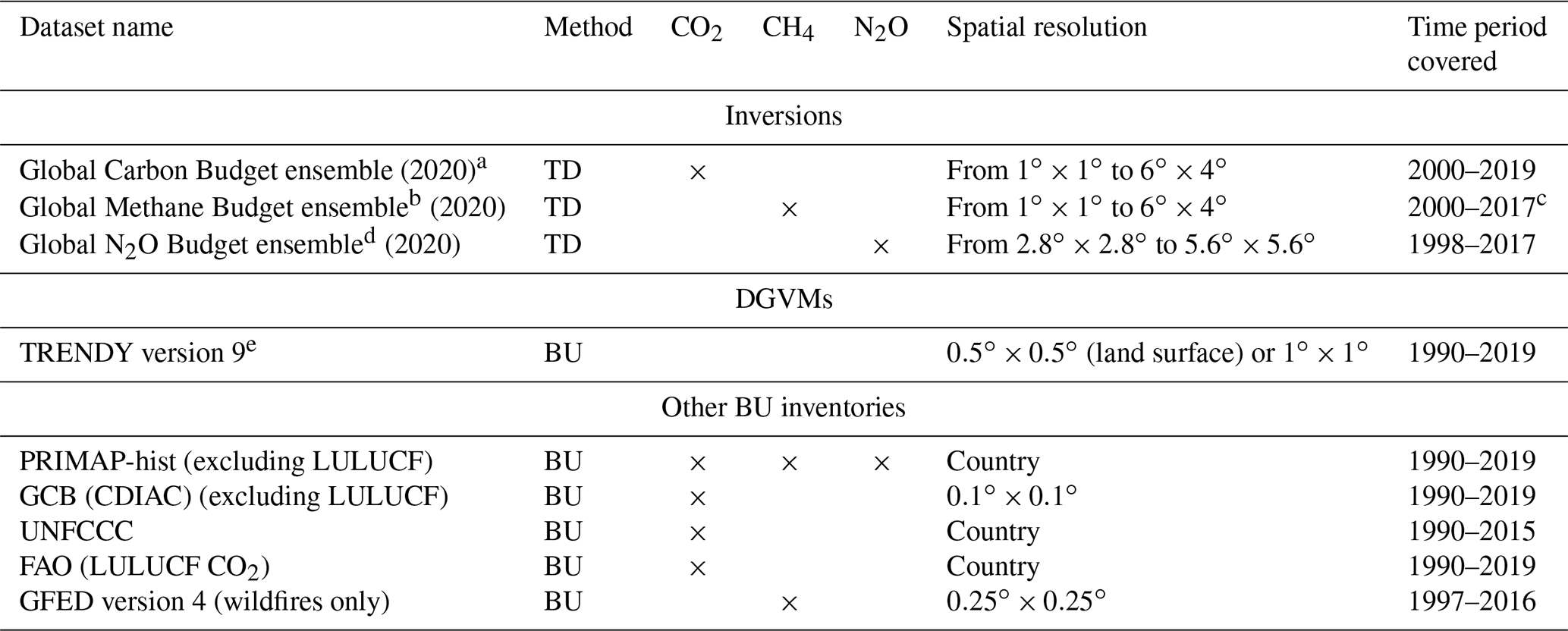
^a See the three inversion details in Table S6. ^b See the 22 inversion details in Table S7. ^c Variations from 2003–2015, 2000–2015 and 2010–2017: see the detailed period coverage for each dataset in Table S7. ^d See the three inversion details in Table S8. ^e See Table S5 for the 14 products.

Table 2 Sectoral reconciliation between the categories defined in the TD and BU methods.

2.1 Regional breakdown

As some countries are small emitters and their area is too small to be resolved by inversions and in some cases even by DGVMs, we grouped African countries into six regions shown in Fig. S2 and listed in Table S2. The grouping followed national borders and biome similarity considering Köppen–Geiger climate zones (Beck et al., 2018), magnitudes of fossil fuel emissions and per capita emissions (Figs. S2, S3 and S8). We also grouped a maximum of about 10 countries per region.

2.2 Inventory datasets

2.2.1 PRIMAP-hist anthropogenic emission assessment for CO₂, CH₄ and N₂O

The PRIMAP-hist version 2.2 BU dataset is derived from Gütschow et al. (2021) and combines UNFCCC reports with a gap-filling method to produce a time series of annual anthropogenic emissions for different IPCC sectors. PRIMAP-hist does not cover the LULUCF sector for CO₂ due to the high uncertainties. PRIMAP-hist does not include emissions from shipping and international aviation but includes cement as part of the FCO₂ emissions. We use data from the HISTCR scenario (data accessed from https://www.pik-potsdam.de/paris-reality-check/primap-hist/, last access: 24 April 2022) from the country-prioritized dataset, which mainly uses UNFCCC (BUR and NC) data unless such data are missing, in which case PRIMAP-hist uses extrapolated data from EDGAR, FAO and the BP Statistical Review of World Energy in their 2021 versions as described in Gütschow et al. (2021).

2.2.2 Global Carbon Project (GCP) fossil CO₂ emissions

We used country-level FCO₂ data published by the global CO₂ budget by the GCP (Friedlingstein et al., 2020) separated per fuel type (gas, oil and coal) and including fossil fuel use in the combined industry, ground transportation and power sectors, natural gas flaring, cement production and process-related emissions (e.g., fertilizers and chemicals). Data for African countries come among others from the CDIAC compiled until 2018 (Gilfillan and Marland, 2021), the BP Statistical Review of World Energy (BP, 2020) and recent estimates of cement production and clinker-to-cement ratios (Andrew, 2020).

2.2.3 UNFCCC inventories for CO₂ in the LULUCF sector

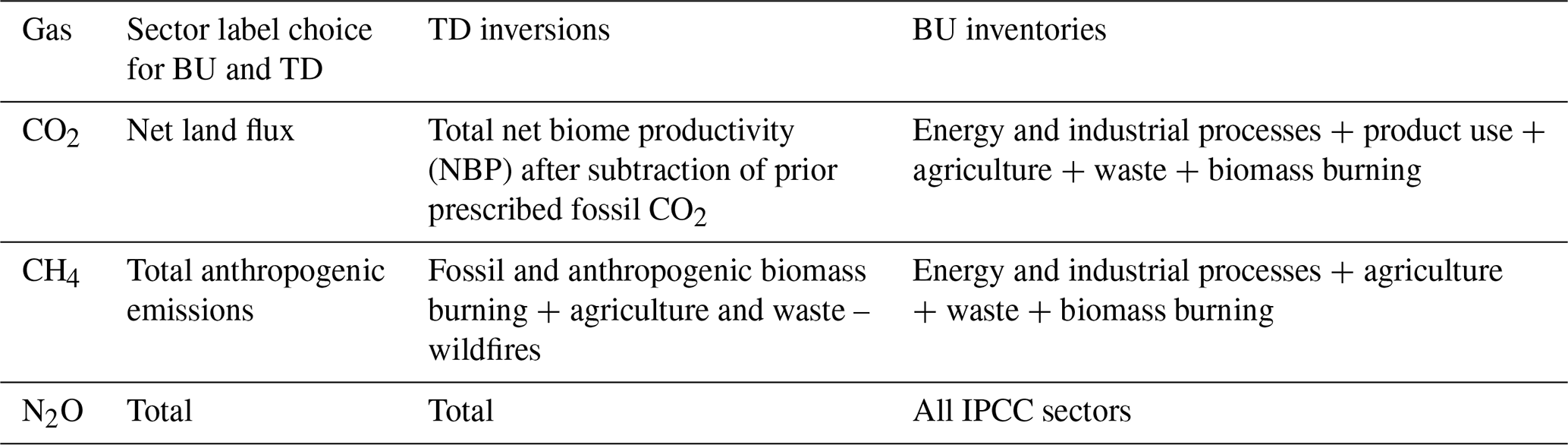
We used UNFCCC submissions for LULUCF CO₂ fluxes from NC and BURs downloaded from the UNFCCC website (https://unfccc.int/, last access: 30 March 2022) in March 2021, and these were further processed into .csv tables by Deng et al. (2022). Those estimates are based on different accounting methods following IPCC guidelines (IPCC, 2019). Country-reported data quality control (QC), quality assurance (QA) and verification processes follow the 2019 IPCC guidelines detailed in the Chapter 6 QA and QC procedures of this document. African countries, being non-Annex I countries, do not report emissions every year. Figure 1 shows the number of BURs and NCs provided each year per African region. The years 1990, 1994, 1995, 2000 and 2005 are characterized by several updates, while most of the other years have few updates. About every 2 years, all the regions have at least one update. Note that flexibility for BURs is given to least developed countries (LDCs), which include 33 out of 56 African countries, and to small island developing states (SIDSs), which include 6 African countries (Table S4).

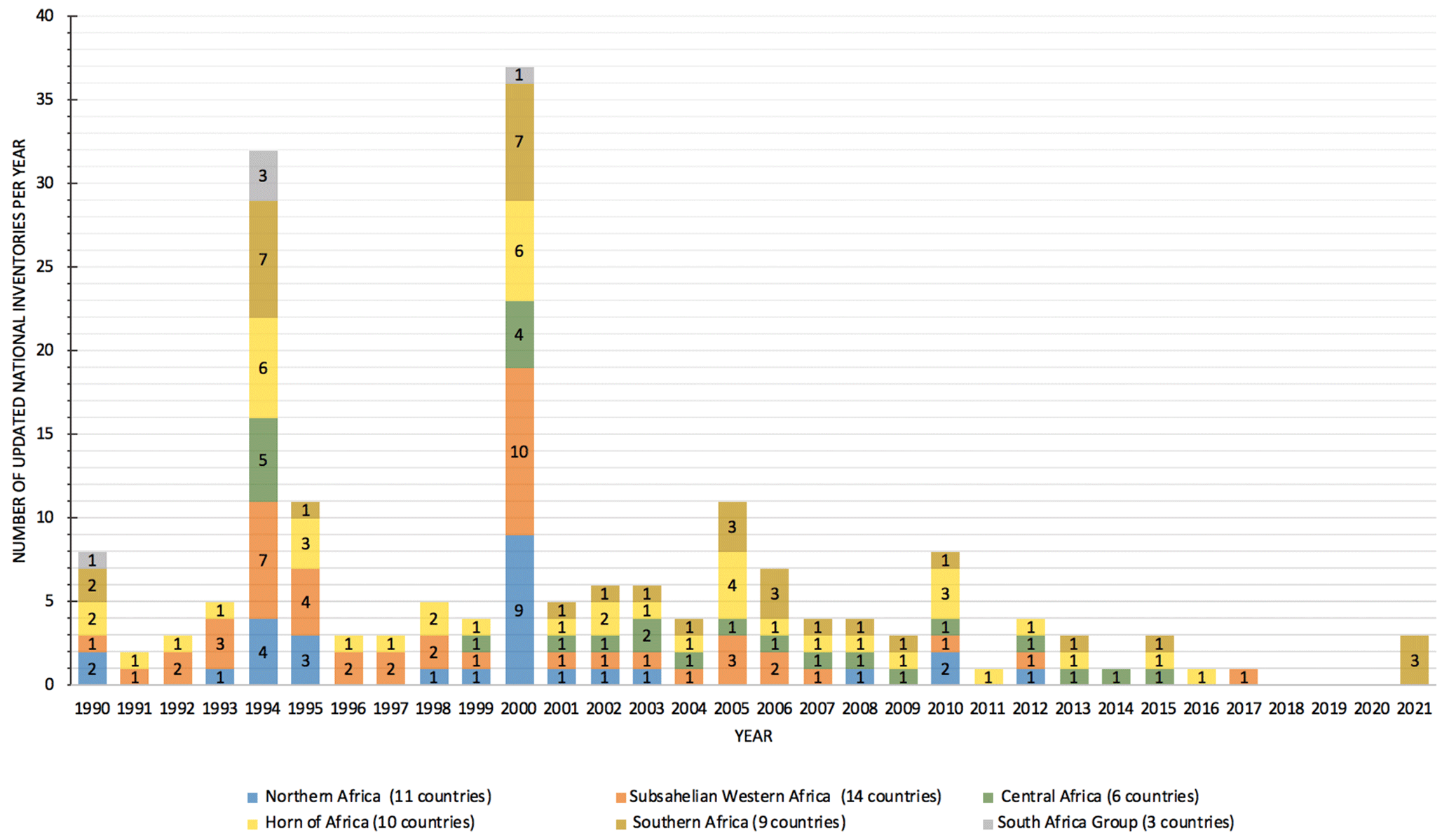
Figure 1 Number of UNFCCC reports for LULUCF CO₂ fluxes in the National Communications and Biennial Update Reports per group of countries defined in Table S2.

Non-Annex I African countries can use older versions of the IPCC guidelines (IPCC, 2006). This induces uncertainties from changes in accounting methods between versions, with recent guidelines having more detailed sectors and sources. There are no data for Libya, Equatorial Guinea, Malawi and Sierra Leone during the whole period. UNFCCC data are missing in some years for Rwanda, Sao Tome and Principe, Senegal, South Sudan and Angola. There are no data for 1990–1998 for Liberia.

We noticed that NCs and BURs lack details regarding the methods used and the sources of activity data and emission factors, and most of them are in the French language. BURs in .pdf format include a non-standardized table for emissions. The reader is sometimes referred to the “national coordinator for climate change service” with no link to any database or contact person.

Because the PA targets human-induced emissions, countries use the proxy of “managed lands” for the LULUCF sector as defined by the IPCC guidelines (IPCC, 2019). Managed lands are areas where LULUCF CO₂ fluxes are assigned to some anthropogenic activities. Several African NCs and BURs do not contain information on their managed land areas. We thus looked at REDD+ national reports (https://redd.unfccc.int/submissions.html?topic=6; last access: 13 August 2022, REDD+, UNFCCC, 2022) to get this information (Fig. S3 and Table S9). LULUCF CO₂ fluxes on managed lands result from either direct anthropogenic effects such as land use change and forestry or from indirect effects (such as change in CO₂ and climate) on land remaining in the same land use, e.g., forest remaining forest (Grassi et al., 2022). The vast majority of African countries use a Tier 1 IPCC accounting method which does not distinguish between these different effects. Tier 1 methods use a classification with only three out of six possible types of land, “forest land”, “cropland” and “grassland”, and do not give spatially explicit land use data. Tier 2 methods include fluxes from six land use types: forest, cropland and grassland, wetlands and urban and other land use for the case of land remaining under the same land use type and for the case of conversions between land use types. In Africa, only South Africa and Zambia used Tier 2 methods for some LULUCF CO₂ subsectors.

2.2.4 Processing of the UNFCCC LULUCF CO₂ data and outlier corrections

We processed the UNFCCC LULUCF CO₂ data for outlier corrections (Table S5). For Guinea-Bissau and Tanzania, we identified inconsistent values from successive communications with substantially differing numbers. For Guinea, Madagascar, Zimbabwe, Congo, Mali, the Central African Republic (CAF), Angola and Mauritius, we identified changes of more than 1 order of magnitude between two consecutive reports and likely implausibly large carbon sinks considering their national forest area. The computations of per area emissions and removals showed discrepancies, which points to the need for further examination and inspection of more recent reports in NDC and REDD+ reports (Table S5). Our corrections explained in the Supplement are consistent with those proposed by Grassi et al. (2022), who diagnosed “biophysically impossible” sequestration rates with a threshold value larger than 10 tCO₂ ha⁻¹ yr⁻¹ over an area greater than 1 Mha. For Namibia, Nigeria and the Democratic Republic of the Congo (DRC), it was challenging to select a best estimate between recent and past reports. For those countries, corrections using more recent data than BURs or NCs have high uncertainties, as noted by Grassi et al. (2022). This includes the absence of any sink for the DRC for instance, in contrast to sinks consistently reported over time and large forested areas in this country's previous reports to the UNFCCC. We therefore systematically looked at corrected values for both case scenarios (with and without Namibia, Nigeria and DRC data corrections). In total, we corrected 13 outliers as shown in Table S5, consistent with Grassi et al. (2022).

2.2.5 FAO LULUCF CO₂ fluxes

We used data from LULUCF CO₂ fluxes over 1990–2019 from the FAO Global Forests Resource Assessments (FAOSTAT, 2021). According to the 2005 FAO categories and definitions, forest is land covering at least 0.5 ha and having vegetation taller than 5 m with a canopy cover higher than 10 %. Other wooded lands refer to land that is not classified as “forest” but is wider than 0.5 ha, that has a canopy cover of 5 %–10 % or that combines trees, shrubs and bushes with a cover higher than 10 %. The FAO data for forests comprise carbon stock changes from both aboveground and belowground living biomass pools. They are independent of country-reported UNFCCC emissions and removals. The FAO estimates are based on activity data, areas of forest land and CO₂ emissions and removal factors. The FAO data report (1) net emissions and removals from “forest land remaining forest land” and from “land converted to forest” grouped together, together with (2) emissions from “net forest conversion”, i.e., deforestation. In contrast, the UNFCCC accounting uses a 20-year window for CO₂ fluxes from land use change, while land use change fluxes from “land converted to forest” are reported separately from those of “forest remaining forest”.

2.3 DGVM datasets

We used the net biome productivity (NBP) from 14 DGVMs from the TRENDY version 9 ensemble covering the period 1990–2019. The different models described in Friedlingstein et al. (2019) are CABLE, CLASS, CLM5, DLEM, ISAM, JSBACH, JULES, LPJ, LPX, OCN, ORCHIDEE-CNP, ORCHIDEE-SDGVM and SURFEX (Table S6). The DGVMs are forced by historical reconstructions of land cover change, atmospheric CO₂ concentration and climate since 1901. Detailed cropland management practices are generally ignored, except for the harvest of crop biomass. Forest harvest is prescribed from historical statistics in 11 models (Table A1 of Friedlingstein et al., 2020). The models simulate carbon stock changes in biomass, litter and soil pools. From the difference between simulations with and without historical land cover change, a flux called “land use emissions” can be obtained from the DGVMs. This flux includes the indirect effects of climate and CO₂ on lands affected by land use change and a foregone sink called “loss or gain of atmospheric sink capacity”, which is absent from the methods used by UNFCCC and FAO. Pongratz et al. (2014) delivered the following definition of loss of sink capacity as “the CO₂ fluxes in response to environmental changes on managed land as compared to potential natural vegetation. Historically, the potential natural vegetation would have provided a foregone sink as compared to human land use.” Thus, land use change fluxes from DGVMs were not compared with other estimates. Note that DGVMs do not explicitly separate managed and unmanaged land. Thus, we used all the forest lands to calculate their mean CO₂ fluxes.

2.4 Atmospheric inversion datasets

2.4.1 CO₂ inversions

We used the net land CO₂ fluxes, excluding fossil fuel emissions (hereafter net ecosystem exchange) from three global inversions of the Global Carbon Project that cover a long period (see Table A4 of Friedlingstein et al., 2020), including CarbonTrackerEurope (CTRACKER-EU-v2019; van der Laan-Luijkx et al., 2017), the Copernicus Atmosphere Monitoring Service (CAMSV18-2-2019; Chevallier et al., 2005) and one variant of Jena CarboScope (JENA, sEXTocNEET_v2020; Rödenbeck, 2005). The GCP inversion protocol recommends using as a fixed prior the same gridded dataset of FCO₂ emissions (GCP-GridFED). However, some modelers used different interpolations of this dataset, and one group used a different gridded dataset (Ciais et al., 2022). We applied a correction to the estimated total CO₂ flux by subtracting a common FCO₂ flux from each inversion (Fig. S1 and the Methodological Supplement S1). The resulting land–atmosphere CO₂ fluxes, or net ecosystem exchange, cannot be directly compared with inventories aiming to assess C stock changes, given the existence of land–atmosphere CO₂ fluxes caused by lateral processes. This issue was discussed by Ciais et al. (2022), and a practical correction of inversions was proposed by Deng et al. (2022) based on new datasets for CO₂ fluxes induced by lateral processes involving river transport, crop and wood product trade. Here we applied the same correction to all the CO₂ inversions.

2.4.2 CH₄ inversions

We used the CH₄ emissions from global inversions over 2000–2017 from the Global Methane Budget (Saunois et al., 2020) (Table 1). This ensemble includes 11 models using GOSAT satellite CH₄ total-column observations covering 2010–2017 and 11 models assimilating surface station data (SURF) since 2000 (Table S5). Surface inversions are constrained by very few stations for Africa, while the GOSAT satellite data have a better coverage. One could thus expect GOSAT inversions to give more robust results. Inversions deliver an estimate of surface net CH₄ emissions, although some of them solve for fluxes in groups of sectors called “super-sectors”. We have not used in situ dataset validation per se: only the GOSAT data were evaluated against the Total Carbon Column Observing Network (TCCON) independent ground-based total column-averaged abundance of CH₄ (XCH₄). In the inversion dataset, net CH₄ surface emissions were interpolated to a $\mathrm{0.8}{}^{\circ }\times {\mathrm{0.8}}^{{}^{\circ }}$ resolution, regridded from coarser-resolution fluxes and separated into super-sectors using either prior emission maps or posterior estimates for those inversions solving fluxes per super-sector following Saunois et al. (2020). More specifically, these five super-sectors are (1) Fossil Fuel, (2) Agriculture and Waste, (3) Wetlands, (4) Biomass and Biofuel Burning (BBUR) and (5) Other natural emissions. We separated CH₄ anthropogenic emissions from inversions using Method 1 and Method 2 proposed by Deng et al. (2022). Method 1 relies on the separation calculated by each inversion except for the BBUR super-sector from which wildfire emissions were subtracted based on GFED version 4 (van der Werf et al., 2017). Method 2 removes from total emissions the median of natural emissions from inversions (Deng et al., 2022). The two methods gave similar results, and only Method 1 was used in the Results section.

2.4.3 N₂O inversions

We used three N₂O atmospheric inversions from the global N₂O budget synthesis (Tian et al., 2020) and from Deng et al. (2022) (Tables S1 and S7): PyVAR CAMS (Thomson et al., 2014), MATCM_JMASTEC (Rodgers, 2000; Patra et al., 2018) and TOMCAT (Wilson et al., 2014; Monks et al., 2017). We used the total N₂O flux from inversions including natural emissions, given that natural emission estimates are highly uncertain for Africa. Inversion results are therefore not directly comparable to the PRIMAP-hist inventory, which only contains anthropogenic emissions.

2.5 Metrics to compare gases and ancillary data and data usage

We express emissions of non-CO₂ gases in megatons of carbon dioxide equivalent (MtCO₂e) using the global warming potential over 100-year time horizon (GWP100) values from the fourth IPCC Assessment Report (IPCC, 2007), consistent with PRIMAP-hist and historical country-reported data. We used AR4 GWP100 because many African countries have been following the 2006 IPCC guidelines referring to AR4 GWP100 2019 refinement in IPCC guidelines, which do not recommend any specific metrics, and therefore we are following the IPCC guidelines used by countries. The multiplicative coefficients to change AR4 to AR6 GWP100 values are 1.19 for fossil CH₄, 1.09 for non-fossil CH₄ and 0.92 for N₂O. We used population data from the United Nations population (United Nations Department of Economic and Social Affairs, Population Division, 2019) to compute per capita FCO₂ emissions and their disparities based on Gini indices (Dorfman et al., 1979) to measure statistical dispersions among a given population (Methodological Supplement S2). We also used African GDP data (World Bank, 2019).

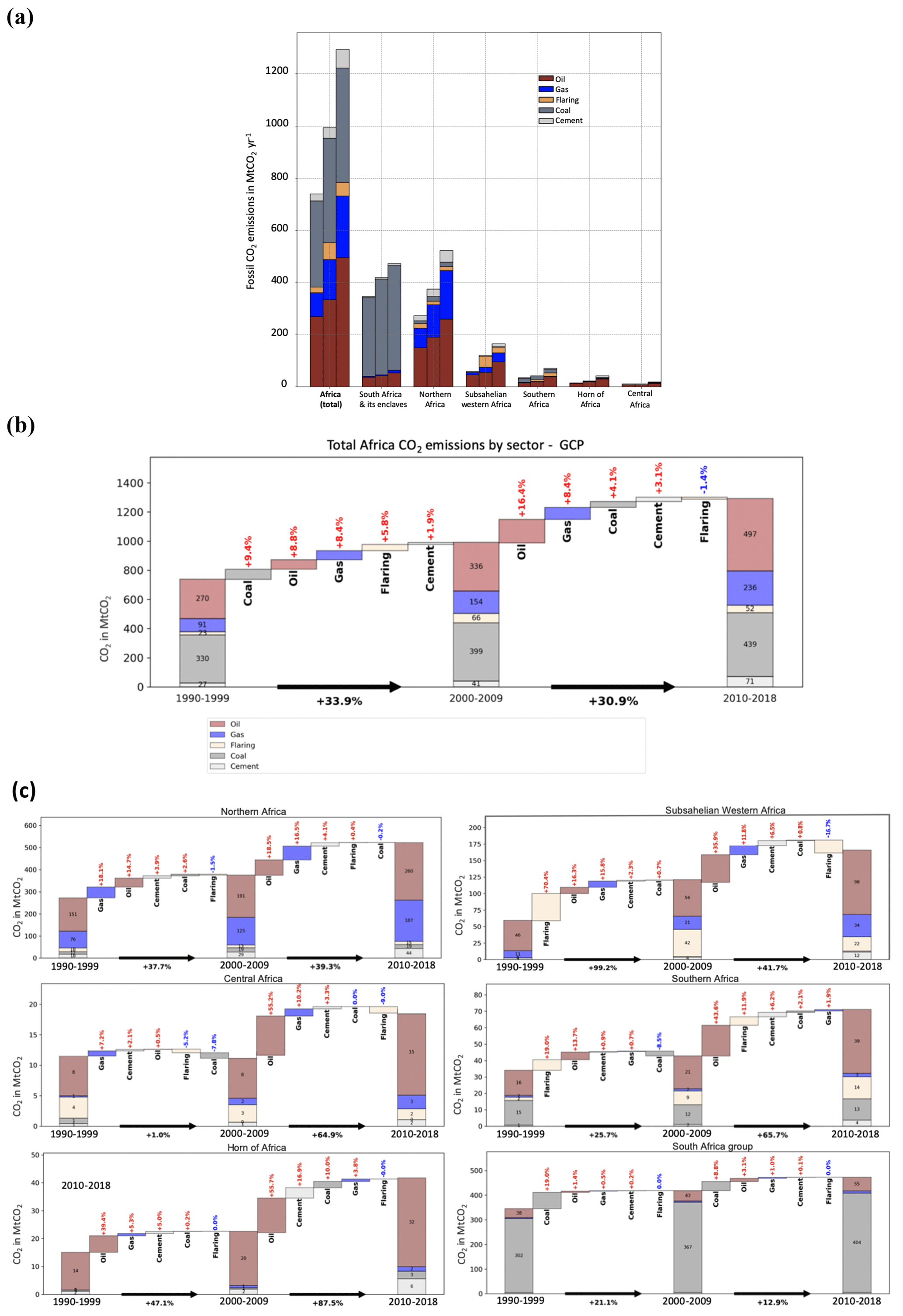
Figure 2 (a) African fossil fuel CO₂ emissions per fuel type and for cement per region over 1990–1999, 2000–2009 and 2010–2018. (b) The contribution of each fuel type to the change in African emissions. (c) The same for different regions, regrouping several countries. Data are from GCP (2019).

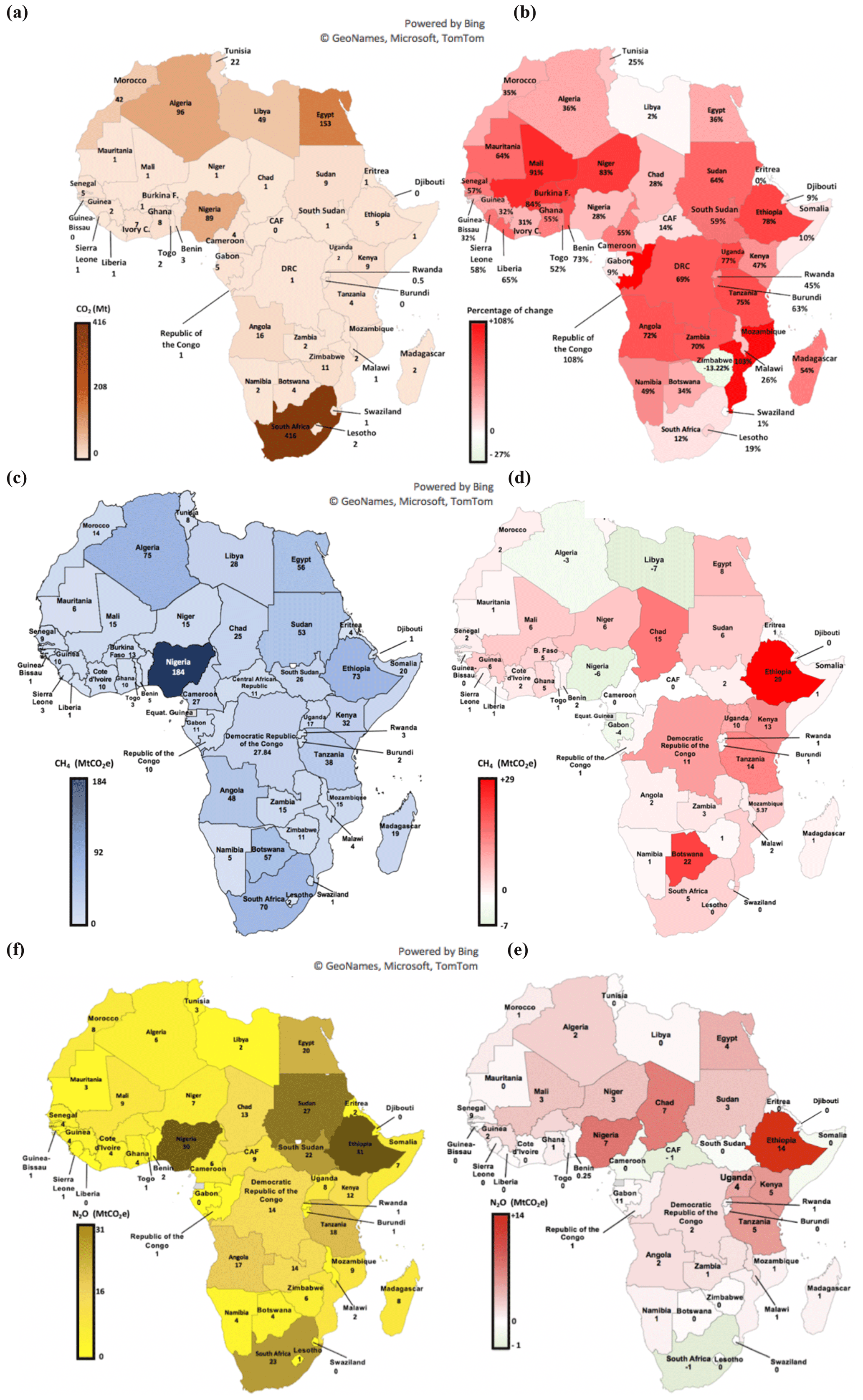
Figure 3 (a) Maps of average fossil fuel CO₂ emissions for African countries during 1999–2008 (Mt CO₂ eq. yr⁻¹) (GCP) and (b) the change from 1999–2008 to 2009–2018 using data from GCP (Friedlingstein et al., 2019) (Mt CO₂ eq. yr⁻¹) expressed as the ratio of the differences in percentage between the FCO₂ for the 1999–2008 total in anthropogenic mean 2009–2018 emissions and mean 1999-2008 emissions (GCP) divided by the average value for both decades. (c–d) The same but with anthropogenic CH₄ emissions from PRIMAP-hist and the differences between the CH₄ mean emissions over 1999–2008 and over 2009–2018 (Mt CO₂ eq. yr⁻¹). (e–f) The same for anthropogenic N₂O emissions from PRIMAP-hist (Mt CO₂ eq. yr⁻¹).

3 Results and discussion

3.1 Fossil CO₂ emissions

3.1.1 Continental, regional and country changes

PRIMAP-hist and GCP

First, we compared GCP and PRIMAP-hist fossil CO₂ emissions. We found that most of the relative differences between these two datasets at country level considerably decreased with time, except for Mali. Those differences are less than 5 % for most of the main African emitters during the last decade, except for South Africa, where the difference is a bit larger than 10 % (see the maps in Fig. S8). The largest relative difference between the two datasets comes from Mali in the decade 2009–2018, with FCO₂ emissions of 3 Mt CO₂ yr⁻¹ in GCP compared to 1 Mt CO₂ yr⁻¹ in PRIMAP-hist. Given the relatively small differences, we chose to use only GCP for trends between decades, but when computing net budgets for the three main GHGs, we show differences between the use of those two estimates.

The changes in African FCO₂ emissions per fuel type and for cement using the GCP data are shown in Fig. 2a. In Fig. 2b, we show absolute values and relative contributions to the total change in each decade. During 2010–2018, total African FCO₂ emissions from oil (497 Mt CO₂ yr⁻¹) and coal (439 Mt CO₂ yr⁻¹) were roughly similar. While global FCO₂ emissions increased by +13 % over this period (Friedlingstein et al., 2019), African FCO₂ almost doubled in 2018 compared to 1990 levels, a relative increase comparable to that of China over the same period. From 1990–1999 to 2000–2009, the mean emissions increased by 33.9 % from 741 to 996 Mt CO₂ yr⁻¹. All FCO₂ sectors contributed to this decadal increase. The contribution from coal (+9.4 %) was slightly larger but comparable to that from oil (+9 %) and gas (+8 %). From 2000–2009 to 2010–2018, emissions further increased by 31 % from 996 to 1295 Mt CO₂ yr⁻¹. The oil and gas fuels contributed the most to this increase, with +16 % for oil and +8 % for gas. Coal emissions increased by only +4.1 %, and coal went from being the first source of African FCO₂ emissions over 2000–2009 to the second one over 2010–2018.

As for the regional contributions to emission changes between 1990–1999 and 2000–2009 shown in Fig. 2b, the main contribution to the total increase came from the region of South Africa, where emissions increased from 302 to 367 Mt CO₂ yr⁻¹ (+21.1 %, coal being the largest contributor). The second largest contribution to the increase is from northern Africa, where oil was the largest contributor (emissions increased from 151 to 191 Mt CO₂ yr⁻¹; +15 %) together with gas (+18 %). The least increasing region was central Africa. Northern Africa experienced the largest increase from 1990–1999 to 2000–2009 and from 2000–2009 to 2010–2018 with successive increases of +38 % and +39 %, largely dominated by oil and gas (Fig. 4b). As a result, during the period 2010–2018, northern African countries were the dominant emitters with 545 Mt CO₂ yr⁻¹. The group of South Africa (including Lesotho and Botswana) was the second biggest emitter region over 2010–2018, mainly due to coal emissions from the Republic of South Africa. The two least contributing African regions were the Horn of Africa and central Africa.

At the country level, Fig. 3a–b show mean FCO₂ emissions and relative changes over the last 2 decades. The main emitters do not have the biggest relative changes. The four main emitters over 2000–2009 were South Africa (416 Mt CO₂ yr⁻¹), Egypt (153 Mt CO₂ yr⁻¹), Algeria (96 Mt CO₂ yr⁻¹) and Nigeria (89 Mt CO₂ yr⁻¹). Those four countries altogether represented 67 % of the continental total emissions over 2000–2009 (987 Mt CO₂ yr⁻¹). The largest relative increases from 2000–2009 to 2010–2018 are from Congo (+108 %), Mozambique (+103 %) and Mali (91 %) compared to relative increases from the main emitters, the Republic of South Africa (+21 %), Egypt (+36 %) and Algeria (+36 %).

3.1.2 Variations of per capita and per GDP fossil fuel CO₂ emissions

Per capita emissions

Using ancillary data on population (Figs. S3 and S4), we computed the mean African per capita emission of 1 tCO₂ per capita per year for 2009–2018, which is 5 times larger than during 1990–1998 (0.2 tC per capita per year) and yet 5 times smaller than the global average (5 tCO₂ per capita per year). From 1999–2008 to 2009–2018, African per capita emissions increased by 30 %. African per capita FCO₂ emissions during 2009–2018 were 17 times less than in the USA (17 tCO₂ per capita per year), 7 times less than in China (7 tCO₂ per capita per year), 7 times less than in the EU27 and UK (7 tCO₂ per capita per year) and 2 times less than in India (2 tCO₂ per capita per year). At the country level, the biggest per capita emissions over 2009–2018 were from the Republic of South Africa with 9 tCO₂ per capita per year, which ranks 14th worldwide, above China and just below Poland. The second biggest per capita emissions were from Libya (8 tCO₂ per capita per year). The smallest ones were from the DRC (0.1 tCO₂ per capita per year). For the first period, 1990–1998, per capita emissions of the African region ranked in this order: South African group (4 tCO₂ per capita per year) > northern Africa (2 tCO₂ per capita per year) > central African countries (1 tCO₂ per capita per year) > southern countries (0.8 tCO₂ per capita per year) > Horn of Africa (0.5 tCO₂ per capita per year) > sub-Sahelian western Africa (0.3 tCO₂ per capita per year). For the second period, 2009–2018, they ranked in this order: South African group (4 tCO₂ per capita per year) > northern Africa (2 tCO₂ per capita per year) > southern countries (1 tCO₂ per capita per year) Horn of Africa (1 tCO₂ per capita per year) > central African countries (1 tCO₂ per capita per year) > sub-Sahelian western Africa (0.4 tCO₂ per capita per year). At the country scale during the first period of 1990–1998, the four African largest per capita emissions ranked in this order: Libya (9 tCO₂ per capita per year > Republic of South Africa (9 tCO₂ per capita per year) > Gabon (5 tCO₂ per capita per year) > Algeria (3 tCO₂ per capita per year). The four African countries with the smallest per capita emissions ranked as follows: Burundi (0.04 tCO₂ per capita per year) < Uganda, Ethiopia and Mali (0.1 tCO₂ per capita per year).

We also computed the Gini index for African per capita FCO₂ emissions for each of the last 3 decades, using data from Friedlingstein et al. (2020) (see Methodological Supplement S2). These Gini values were 0.7 for 1990–1998, 0.7 for 1999–2008 and 0.7 for 2009–2018 and thus were very stable over the last 30 years and close to 1, indicating high inequities among countries.

Emissions per GDP

Per exchange rate vs. per purchasing power parity (PPP) GDP

According to the International Monetary Fund (IMF), the GDP delivers an estimate “of the monetary value of goods and services produced in a country over a chosen period.” GDP data from the World Bank (2019) are available for 30 African countries only (Fig. S5). The four countries with the biggest GDP expressed in US Dollars (exchange rate GDP) (Fig. S6) are Nigeria (USD 490B) > South Africa (USD 350B) > Egypt (USD 330B) and Algeria (USD 330B) > Angola (USD 120B). The four countries with the smallest GDP in 2015 are Gambia (USD 1.4B) and Seychelles (USD 1.4B) > Guinea-Bissau (USD 1B) > Comoros (USD 970M). Emissions per USD GDP are shown in Fig. S6. The PPP calculated by the International Comparison Program (ICP) of the World Bank is a refined measure of what a given national currency can acquire in terms of goods or services in another country, removing the impact of currency exchange rates. Emissions per PPP USD GDP are shown in Fig. S7.

The mean of African emissions per unit PPP USD GDP in 2016 was 0.6 kgCO₂ per PPP USD per year, which is more than 2 times the global value and 3 times the mean value of the USA (0.2 kgCO₂ per PPP USD per year) and Europe (0.2 kgCO₂ per PPP USD per yr⁻¹). This points to more carbon-intensive economic growth in Africa than in developed countries, which may be an important barrier to future mitigation strategies as the GDP of Africa has grown by 112 % in the last 30 years and is projected to increase in the future by 3 % per year (World Bank, 2022). At the regional level, the largest values were from South Africa (0.4 kgCO₂ per PPP USD per year) > northern Africa, southern countries and Sahelian western Africa (0.2 kgCO₂ per PPP USD per year) > central Africa and the Horn of Africa (0.1 kgCO₂/PPP USD of GDP). At the country scale, the largest emitters per unit of GDP were Libya (0.7 kgCO₂ per PPP USD per year) and South Africa (0.7 kgCO₂ per PPP USD per year) > Lesotho (0.4 kgCO₂ per PPP USD per year) > Algeria (0.3 kgCO₂ per PPP USD per year) (Fig. S7). The smallest emitters were the DRC (0.03 kgCO₂ per PPP USD per yr⁻¹) <(0.04 kgCO₂ per PPP USD per year) < Burundi (0.06 kgCO₂ per PPP USD per year) < Uganda (0.07 kgCO₂ per PPP USD per year).

We also used GDP per unit exchange rate from the IMF (2020). The mean African emission per unit of GDP_exch.rate was 0.5 kgCO₂ per USD per year, larger than elsewhere, except in Asia (0.6 kgCO₂ per GDP_exch.rate per year. As shown in Fig. S6, over 2013–2017 the six biggest emitters were South Africa (0.7 kgCO₂ per GDP_exch.rate per year) > Libya (0.5 kgCO₂ per GDP_exch.rate per year) > South Sudan (0.4 kgCO₂ per GDP_exch.rate per year) > Zimbabwe, Benin and Algeria (0.3 kgCO₂ per GDP_exch.rate per year). The correlation coefficient between GDP_exch.rate and FCO₂ emissions per GDP_exch.rate was 0.3, suggesting that countries with a high GDP do not always emit more CO₂ per unit GDP. For instance, South Africa ranked first with 0.7 kgCO₂ per GDP_exch.rate per year and second for GDP (USD 350 billion), and Nigeria ranked first for GDP (USD 490 billion) but 21st for emissions per GDP (0.1 kgCO₂ per GDP_exch.rate per year). This may be related to the fact that countries with a high GDP are also more likely to create growth through sustainable activities.

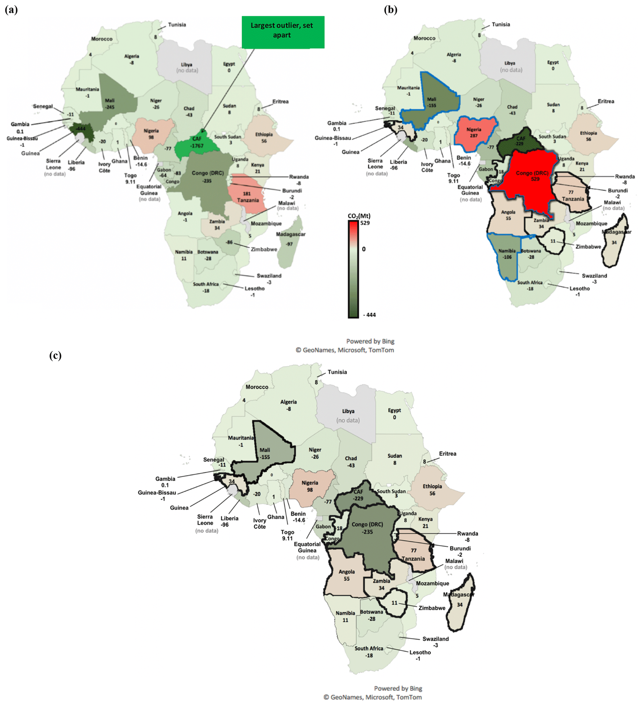
Figure 4 Map of national LULUCF CO₂ fluxes for 2001–2018 (Mt CO₂ yr⁻¹). (a) Before outlier removal. (b) After outlier removal according to Grassi et al. (2022). (c) After the outlier removal (DRC, Namibia and Nigeria) from this study. Positive values represent a net C loss by ecosystems.

3.2 LULUCF CO₂ fluxes

3.2.1 Outlier corrections

In this section, we analyze CO₂ fluxes from the LULUCF sector based on UNFCCC data (Sect. 1.1), which include forest lands, grasslands, croplands and all possible conversions between them (IPCC, 2003). As shown in Sect. 1.2 and Table S4, we found that some countries' reports are outliers with biophysically implausible CO₂ sinks and/or sudden unexplained very large changes between successive reports. Due to scarce data over 1990–1998, we focus on the period 2001–2018. In the following paragraph, we discuss four approaches to including UNFCCC data: (a) uncorrected data, (b) corrections following Grassi et al. (2022) for all countries, (c) corrections following Grassi et al. (2022) except for the DRC, Namibia and Nigeria and (d) corrections following Grassi et al. (2022) except for the DRC.

Figure 4a shows UNFCCC data without correcting for outliers, based on BUR and NC data accessed in May 2022. The majority of the countries are sinks or small sources, except Tanzania and Nigeria, which are large sources. Very large (implausible) sinks are seen in Guinea and CAF. The continent is a CO₂ sink of −3309 Mt CO₂ yr⁻¹ during the period 2001–2018.

Figure 4b shows the corrected fluxes according to Grassi et al. (2022), who excluded implausible large sink rates and used NDC and REDD+ reports instead of NC data for the DRC, Congo, CAF, Guinea and Madagascar and the most recent BUR, NC and inventory data for Namibia, Angola, Zimbabwe and Nigeria (see their Table 7). Africa as a whole is a CO₂ source of 265 Mt CO₂ yr⁻¹. At a regional scale, the mean CO₂ sources are distributed as follows in four regions: sub-Sahelian western Africa (235 Mt CO₂ yr⁻¹) > Horn of Africa (153 Mt CO₂ yr⁻¹) > central Africa (144 Mt CO₂ yr⁻¹) > southern Africa (14 Mt CO₂ yr⁻¹). The two sink regions are northern Africa (−259 Mt CO₂ yr⁻¹) and South Africa (−23 Mt CO₂ yr⁻¹). At the country scale, after the corrections of Grassi et al. (2022), the four countries with the larger sinks are CAF (−229 Mt CO₂ yr⁻¹) > Mali (−155 Mt CO₂ yr⁻¹) > Namibia (−106 Mt CO₂ yr⁻¹) > Cameroon (−77 Mt CO₂ yr⁻¹). The four countries with the largest sources are the DRC (529 Mt CO₂ yr⁻¹) > Nigeria (287 Mt CO₂ yr⁻¹) > Tanzania (77 Mt CO₂ yr⁻¹) > Ethiopia (56 Mt CO₂ yr⁻¹). The main issue with the correction from Grassi is that it reports no sink in the DRC, which has an important forest coverage representing 68 % of the country's area (FAO, 2020) and for which a sink was consistently reported in previous NCs.

Figure 4c shows LULUCF CO₂ in African countries that is consistent with Grassi et al. (2022) except for three countries: Namibia (we used 2000 NC3 instead of NIR2019), Nigeria (we used 2014 NC2 instead of 2017 BUR2) and the DRC (we used 2015 NC3 instead of 2021 NDC). In that approach, Africa becomes a net CO₂ sink of −589 Mt yr⁻¹ over 2001–2018. At the regional scale, the region of central Africa (−620 Mt CO₂) remains the main sink. However, the values and ranking of the top sources are Horn of Africa (153 Mt CO₂) > southern Africa (141 Mt CO₂) > sub-Sahelian western Africa (19 Mt CO₂). At the country scale with this correction choice, the top sinks are the DRC (−235 Mt CO₂) > CAF (−229 Mt CO₂) > Mali (−155 Mt CO₂), and the top three sources are Nigeria (98 Mt CO₂) > Tanzania (77 Mt CO₂) > Ethiopia (56 Mt CO₂).

In the fourth approach, where we use the corrections of Grassi et al. (2022) except for the DRC and where we kept the latest national communication instead of the most recent NDC, the continent is a net sink of −504 Mt CO₂ yr⁻¹ over 2001–2018. At the regional scale, central Africa is a large CO₂ sink, and the ranking of the sink regions is the central African group (−620 Mt CO₂ yr⁻¹) > northern Africa (−259 Mt CO₂ yr⁻¹) > South Africa (−23 Mt CO₂ yr⁻¹). The ranking of the source regions stays unchanged. At the country scale, the main sink is the DRC (−235 Mt CO₂ yr⁻¹). In this paper, we will mainly use data corrected following Grassi et al. (2022), but we want to raise a cautionary flag that adopting their correction for the DRC had an enormous effect on the CO₂ budget of the continent, which becomes a source. Using the original latest national communication of the DRC instead of the NDC used by Grassi et al. (2022) and our own corrections for Namibia and Nigeria instead of those of Grassi et al. (2022) increased the continental CO₂ uptake.

3.2.2 Comparison of UNFCCC-managed land area and FAO forest and other wooded land areas

Figure S10 shows a comparison of land areas in the NC, BUR and REDD+ reports (https://redd.unfccc.int/submissions.html?mode=browse-bycountry, last access: 24 June 2022) with FAO forest land areas (2015) and FAO forest land and other woodland areas for the year 2015 (see Table S9). Consistent with Grassi et al. (2022), all forest lands in Africa are considered to be managed. We found that FAO forest land areas are closer to UNFCCC estimates than the sum of FAO forest and other woodland areas, except for the DRC, Sudan, Senegal, Niger and Mauritania (Table S9). Forest areas in UNFCCC data using the IPCC default method do not exactly match FAO data estimates of forest areas.

3.2.3 LULUCF CO₂ fluxes from UNFCCC vs. DGVMs and inversions

A comparison between LULUCF CO₂ fluxes from UNFCCC, FAO, DGVMs and inversions is shown in Fig. 5 at the scale of the continent and for the six regions. The period of overlapping time series is 2001–2018. For the continent, DGVMs give a mean sink of −232 Mt CO₂ yr⁻¹ with a huge range from −1977 to 2095 Mt CO₂ yr⁻¹. The years with the biggest sinks for DGVMs (from the median of all the models) are 2006 and 2018, and the years with the smallest sinks are 2005 and 2016, which seem to be related to widespread drought years across Africa. A key result shown by this figure is that the DGVMs and inversions show a huge spread, making them of little value for “verifying” inventories for LULUCF CO₂ fluxes in Africa. However, we observed that the medians of all the DGVMs point to a sink for Africa, unlike the UNFCCC data with the correction from Grassi et al. (2022).

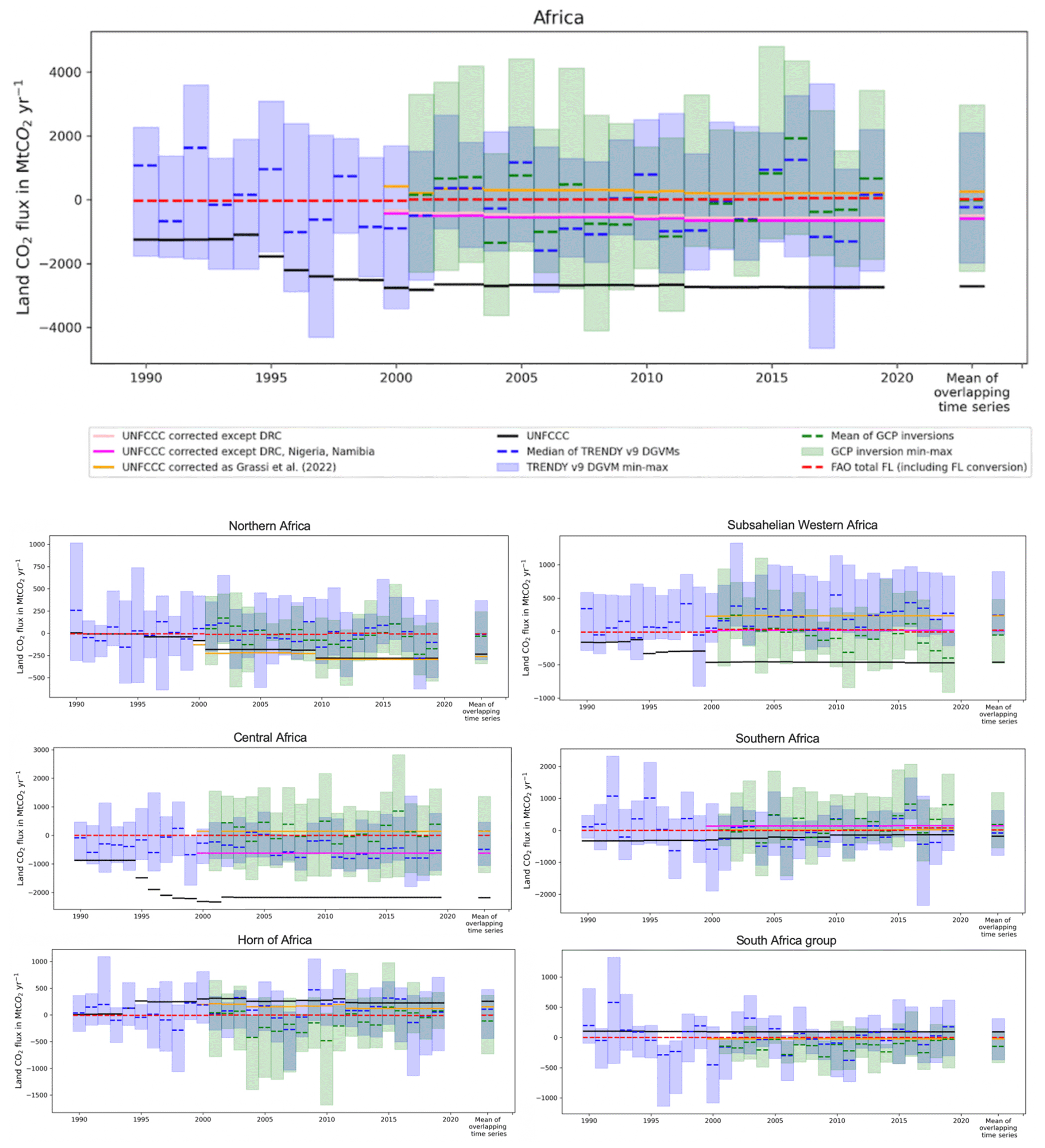
Figure 5 LULUCF CO₂ emissions and sinks: comparison between UNFCCC national greenhouse gas inventories, TRENDY version 9 DGVMs and inversions for the whole of Africa and for each of the six African subregions, and country details for the three main outliers (MtCO₂ yr⁻¹). Shaded green areas represent the minimum and maximum ranges from the inversions. Shaded blue represents the minimum and maximum ranges for TRENDY version 9 DGVMs. Green dashes denote the mean of the inversions, blue dashes denote the median of TRENDY version 9 DGVMs and green dashes denote the median of the inversions. Positive values represent a source, while negative values refer to a sink.

For three large countries, corrected UNFCCC values from Grassi et al. (2022) show a bigger discrepancy with other BU and TD methods than uncorrected ones (Fig. S9). In Namibia the corrected value gives a larger sink compared to other methods, while the uncorrected value is comparable. In the DRC, the corrected value, which was a source, seems a high overestimation compared to the other methods, while the uncorrected UNFCCC value is close to median values from inversions and to the FAO. In Nigeria, the corrected value seems to be a high overestimation of a net source compared to the other methods, pointing to either a smaller source (FAO, inversions) or even a sink (DGVMs).

The data in Fig. 5 show that most of the methods agree on a small net sink for African LULUCF CO₂ fluxes, except for corrections following Grassi et al. (2022). However, disagreements exist among the different methods. Inversions give a smaller net sink (${\mathrm{mean}}_{\min }^{\max }$) of $-{\mathrm{14}}_{-\mathrm{2248}}^{\mathrm{2966}}$ Mt CO₂ yr⁻¹ than DGVMs ($-{\mathrm{232}}_{-\mathrm{1978}}^{\mathrm{2095}}$ Mt CO₂ yr⁻¹). The median value of the inversions is nevertheless within the range of the DGVMs. At the scale of Africa, the inversions' mean sink is ∼12 times smaller than the median from the DGVMs. The min–max range of the inversions (5216 Mt CO₂ yr⁻¹) is larger than the range of the DGVMs by 17 %. The DGVMs and inversions show a positive temporal correlation coefficient (r=0.7) for annual trends (linear fit to the time series).

UNFCCC values with the fourth approach point to a net sink (−503 Mt CO₂ yr⁻¹), similar to the third one. Corrected values as in Grassi et al. (2022) give a net source estimate of 265 Mt CO₂ yr⁻¹. FAO net emissions and removals represent a small net source (18 Mt CO₂ yr⁻¹). Differences between FAO and UNFCCC, as explained in Grassi et al. (2022), could be due to the fact that FAO estimates of CO₂ fluxes for forest remaining forest can be set to zero in the absence of any national stock change inventory (Table 3).

Table 3 Mean net LULUCF CO₂ (emissions and removals) over the overlapping period of the different datasets (2001–2018) (MtCO₂ yr⁻¹).

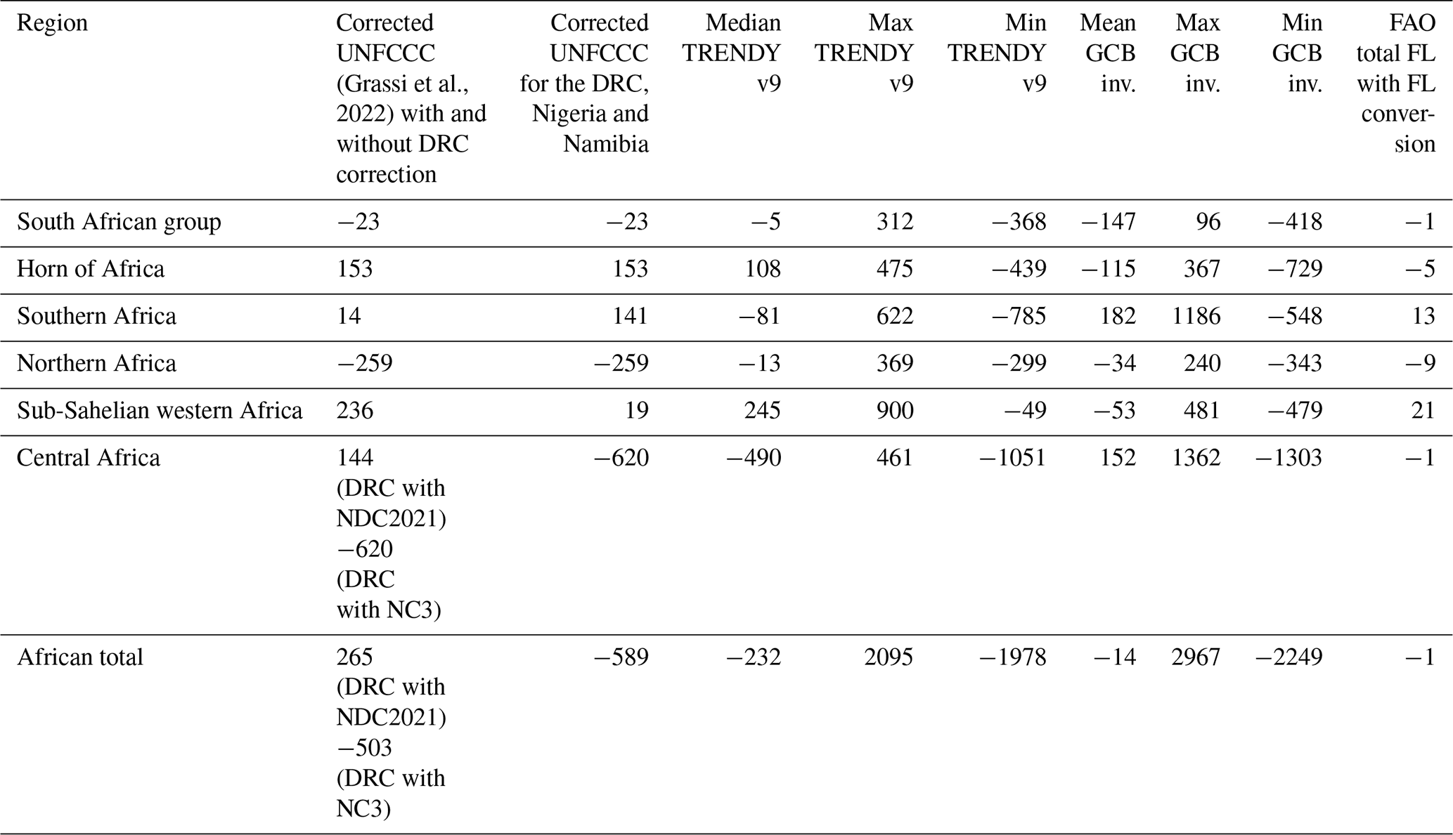
At the regional scale, we note some agreement between the different BU approaches. First, for the South African region, the mean of the DGVM medians during the overlapping period 2001–2018 (−5 Mt CO₂ yr⁻¹) and the FAO estimate (−1 Mt CO₂ yr⁻¹) are comparable and not too far from Grassi et al. (2022) (−23 Mt CO₂ yr⁻¹). Second, for northern Africa, the DGVM median (−13 Mt CO₂ yr⁻¹) and the FAO mean estimate over the same period (−9 Mt CO₂ yr⁻¹) are comparable. Finally, in sub-Sahelian western Africa, the DGVM (236 Mt CO₂ yr⁻¹) and UNFCCC corrected following Grassi et al. (2022) (245 Mt CO₂ yr⁻¹) are also close to each other.

Northern Africa is the group where DGVMs and inversions point to the closest values in terms of both signs (sinks) and magnitudes with small sinks of $-{\mathrm{13}}_{-\mathrm{299}}^{\mathrm{369}}$ and $-{\mathrm{34}}_{-\mathrm{343}}^{\mathrm{240}}$ Mt CO₂ yr⁻¹, respectively.

Looking at DGVMs and inversions in the region of South Africa, we found that both DGVMs and inversions point to a sink ($-{\mathrm{5}}_{-\mathrm{368}}^{\mathrm{312}}$ and $-{\mathrm{147}}_{-\mathrm{418}}^{\mathrm{96}}$ Mt CO₂ yr⁻¹, respectively), with however a different magnitude. The region showing the highest discrepancies between inversions and DGVM values is central Africa with a source for inversions (${\mathrm{152}}_{-\mathrm{1303}}^{\mathrm{1362}}$ Mt CO₂ yr⁻¹) and a sink for DGVMs ($-{\mathrm{490}}_{-\mathrm{1051}}^{\mathrm{461}}$ Mt CO₂ yr⁻¹). Sub-Sahelian western Africa also shows discrepancies in both sign and magnitude with ${\mathrm{245}}_{-\mathrm{49}}^{\mathrm{900}}$ Mt CO₂ yr⁻¹ for DGVMs and $-{\mathrm{53}}_{-\mathrm{479}}^{\mathrm{481}}$ Mt CO₂ yr⁻¹ for inversions. The same is true for southern Africa with $-{\mathrm{81}}_{-\mathrm{785}}^{\mathrm{622}}$ Mt CO₂ yr⁻¹ for DGMVs and ${\mathrm{182}}_{-\mathrm{548}}^{\mathrm{1186}}$ Mt CO₂ yr⁻¹ for inversions as well as the Horn of Africa with ${\mathrm{108}}_{-\mathrm{439}}^{\mathrm{475}}$ Mt CO₂ yr⁻¹ for DGVMs and $-{\mathrm{115}}_{-\mathrm{729}}^{\mathrm{367}}$ Mt CO₂ yr⁻¹ for inversions. At the regional scale, the inversions systematically give smaller sinks than DGVMs in the regions of central Africa, sub-Sahelian western Africa and northern Africa after 2010 (Fig. 5).

We also computed the correlation coefficient at the regional level between DGVM and inversion trends for each region. The highest correlation coefficients are in the South African region (r=0.7), followed by northern Africa (r=0.6) and southern Africa (r=0.5). The lowest correlation coefficients are for the group of central African countries (r=0.3), sub-Sahelian western African countries (r=0.2) and the Horn of Africa (r=0.1).

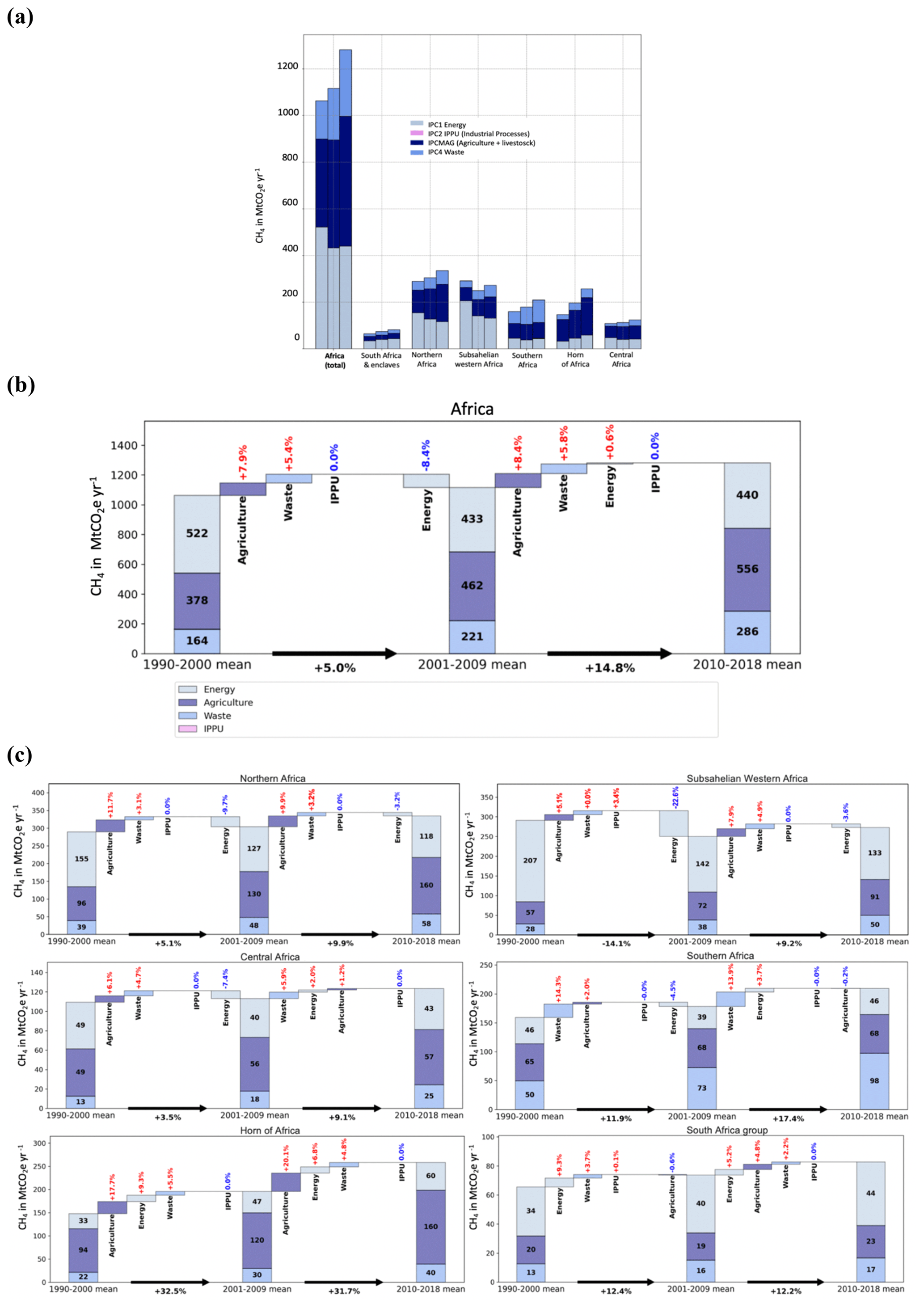
Figure 6 (a) African mean anthropogenic CH₄ emissions (MtCO₂e yr⁻¹) over 3 decades (1990–1998, 1999–2008 and 2010–2018). (b) The contributions of each sector to the change in African emissions in the last 3 decades. (c) The same for different regions, regrouping several countries. Data are from PRIMAP-hist (2021).

3.3 CH₄ anthropogenic emissions

3.3.1 Total and sectoral bottom-up CH₄ anthropogenic emissions and decadal changes

Figure 6 shows anthropogenic CH₄ emissions from PRIMAP-hist grouped into four super-sectors (see Sect. 1). A map of CH₄ emissions and their trends per country is given in Fig. 3c–d. LULUCF CH₄ emissions are not considered in PRIMAP-hist. African anthropogenic CH₄ emissions sum up to 1154 Mt CO₂ eq. yr⁻¹ over the last 3 decades. They increased from 1064 Mt CO₂ eq. yr⁻¹ in 1990–2000 to 1116 Mt CO₂ eq. yr⁻¹ in 2001–2009 and further to 1282 Mt CO₂ eq. yr⁻¹ over 2010–2018 (Fig. 6a). Over the last 3 decades, the main African CH₄-emitting super-sectors shifted from Energy (49 % over 1990–2000) to Agriculture, mainly due to a northern African contribution. At the regional level, the main contributing region to the total emissions shifted over the last 30 years from sub-Sahelian western Africa (297 Mt CO₂ eq. yr⁻¹ for all sectors in 1990–2000) to northern Africa (333 Mt CO₂ eq. yr⁻¹ for all sectors in 2010–2018).

Northern African emissions increased from 290 Mt CO₂ eq. yr⁻¹ in 1990–2000 to 305 Mt CO₂eq yr⁻¹ in 2001–2009 and further to 333 Mt CO₂ eq. yr⁻¹ in 2010–2018. Sub-Sahelian emissions decreased from 297 Mt CO₂ eq. yr⁻¹ in 1990–2000 to 252 Mt CO₂ eq. yr⁻¹ in 2001–2009 and re-increased to 274 Mt CO₂ eq. yr⁻¹ in 2010–2018, a level lower than in the first decade (Fig. 6b). The Horn of Africa emissions increased from 149 Mt CO₂ eq. yr⁻¹ over 1990–2000 to 197 Mt CO₂ eq. yr⁻¹ over 2001–2009 and further to 260 Mt CO₂ eq. yr⁻¹ over 2010–2018. The emissions from southern Africa increased from 184 Mt CO₂ eq. yr⁻¹ in 1990–2000 to 180 Mt CO₂ eq. yr⁻¹ in 2001–2009 and further to 212 Mt CO₂ eq. yr⁻¹ in 2010–2018. Emissions from the central African region increased from 111 Mt CO₂ eq. yr⁻¹ in 1990–2000 to 114 Mt CO₂ eq. yr⁻¹ in 2001–2009 and further to 125 Mt CO₂ eq. yr⁻¹ in 2010–2018. We also computed the Gini indices of African countries' anthropogenic CH₄ per capita emissions and obtained the following values: 0.6 in 1990–1998, 0.5 in 1999–2008 and 0.5 in 2009–2018, i.e., with a trend of increasing “inequality” between countries. As compared to per capita FCO₂ emissions, more homogeneity is observed for CH₄ per capita emissions. Similar to FCO₂ emissions, the Gini values remained stable over the 3 decades, showing a similar level of inequality over time.

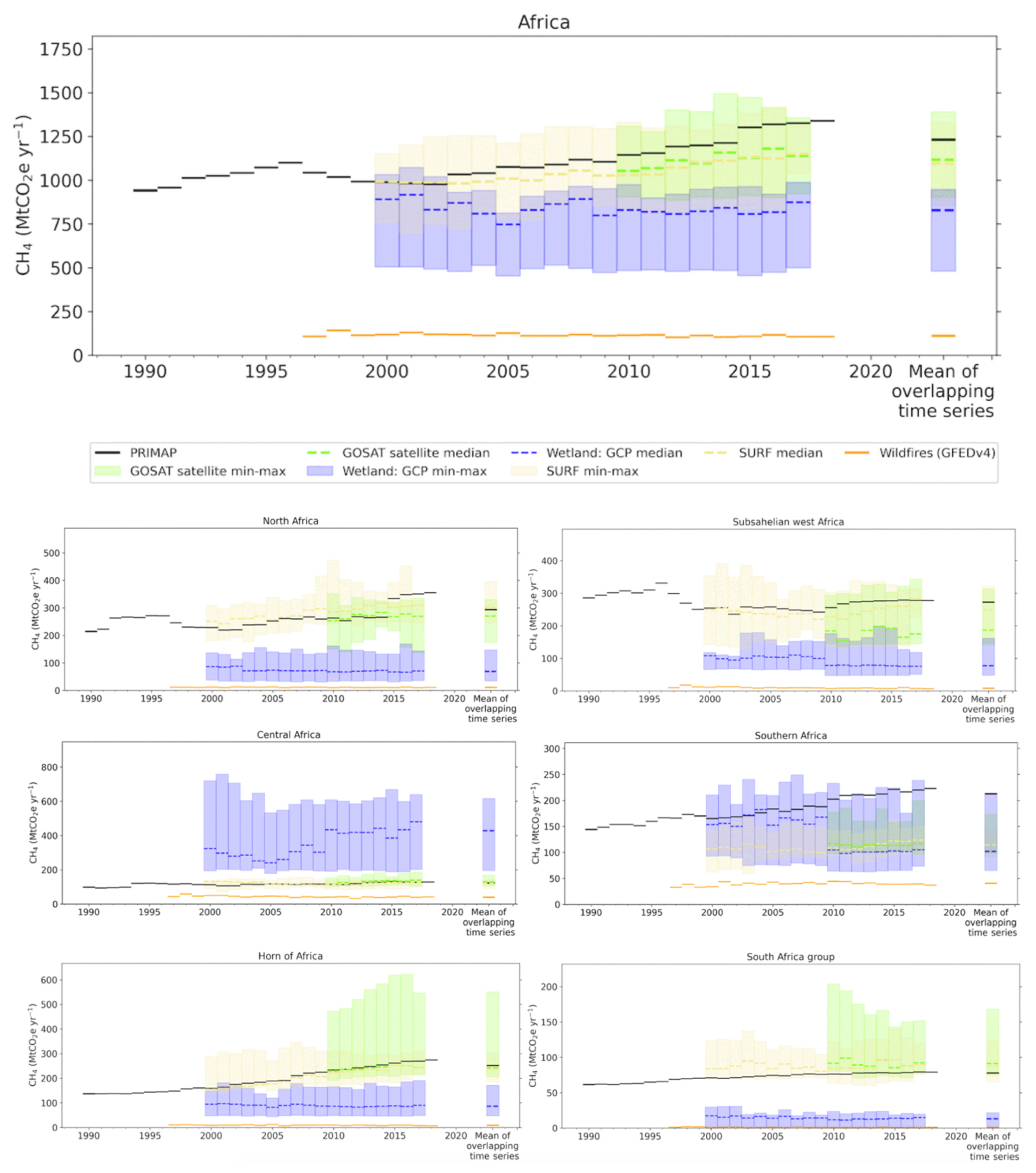
Figure 7 Comparison of the total anthropogenic CH₄ emissions (MtCO₂e yr⁻¹) from the PRIMAP-hist inventory (black) and global inversions. The shaded green and yellow areas represent the minimum and maximum range from GOSAT satellite and surface inversions, respectively. The shaded blue areas represent the minimum and maximum range of wetland natural emissions from inversions. The orange lines represent wildfire emissions from GFED version 4.

3.3.2 BU vs. inversions for total and anthropogenic CH₄ emissions

Figure 7 compares BU anthropogenic emissions from PRIMAP-hist for the period 2000–2018 with the inversions' anthropogenic emissions (see Sect. 1). Wetland natural emissions are shown in the figure only for information from the median and range of the inversions. Over the overlapping time period, medians of both GOSAT and surface inversions are always smaller than PRIMAP-hist emissions at the continental and regional levels, except for the central African region. For the African continent, the mean, minimum and maximum of GOSAT inversions for anthropogenic CH₄ emissions over 2000–2018 are ${\mathrm{1117}}_{\mathrm{903}}^{\mathrm{1390}}$ Mt CO₂ eq. yr⁻¹, very close to the mean of surface inversions of ${\mathrm{1094}}_{\mathrm{853}}^{\mathrm{1330}}$ Mt CO₂ eq. yr⁻¹. Good agreement between GOSAT and surface inversions was also found in other high-emitting countries (Deng et al., 2022). In contrast, PRIMAP-hist gives a mean of CH₄ anthropogenic emissions of 1231 Mt CO₂ eq. yr⁻¹ over the period 2010–2017. The mean wetland flux from inversions over 2010–2017 is ${\mathrm{827}}_{\mathrm{481}}^{\mathrm{946}}$ Mt CO₂ eq. yr⁻¹. Methane emissions from wildfires over Africa for the same period are less important, with a mean of 110 Mt CO₂ eq. yr⁻¹.

The regional emissions from PRIMAP-hist ranked in decreasing order are northern Africa (293 Mt CO₂ eq. yr⁻¹) > sub-Sahelian western Africa (272 Mt CO₂ eq. yr⁻¹) > Horn of Africa (252 Mt CO₂ eq. yr⁻¹) > southern Africa (212 Mt CO₂ eq. yr⁻¹) > central Africa (123 Mt CO₂ eq. yr⁻¹) > South Africa (78 Mt CO₂ eq. yr⁻¹). For both GOSAT and surface inversions, the ranking of the regions (Table S11) is almost the same for surface inversions and PRIMAP-hist, with the exception of central Africa and southern Africa.

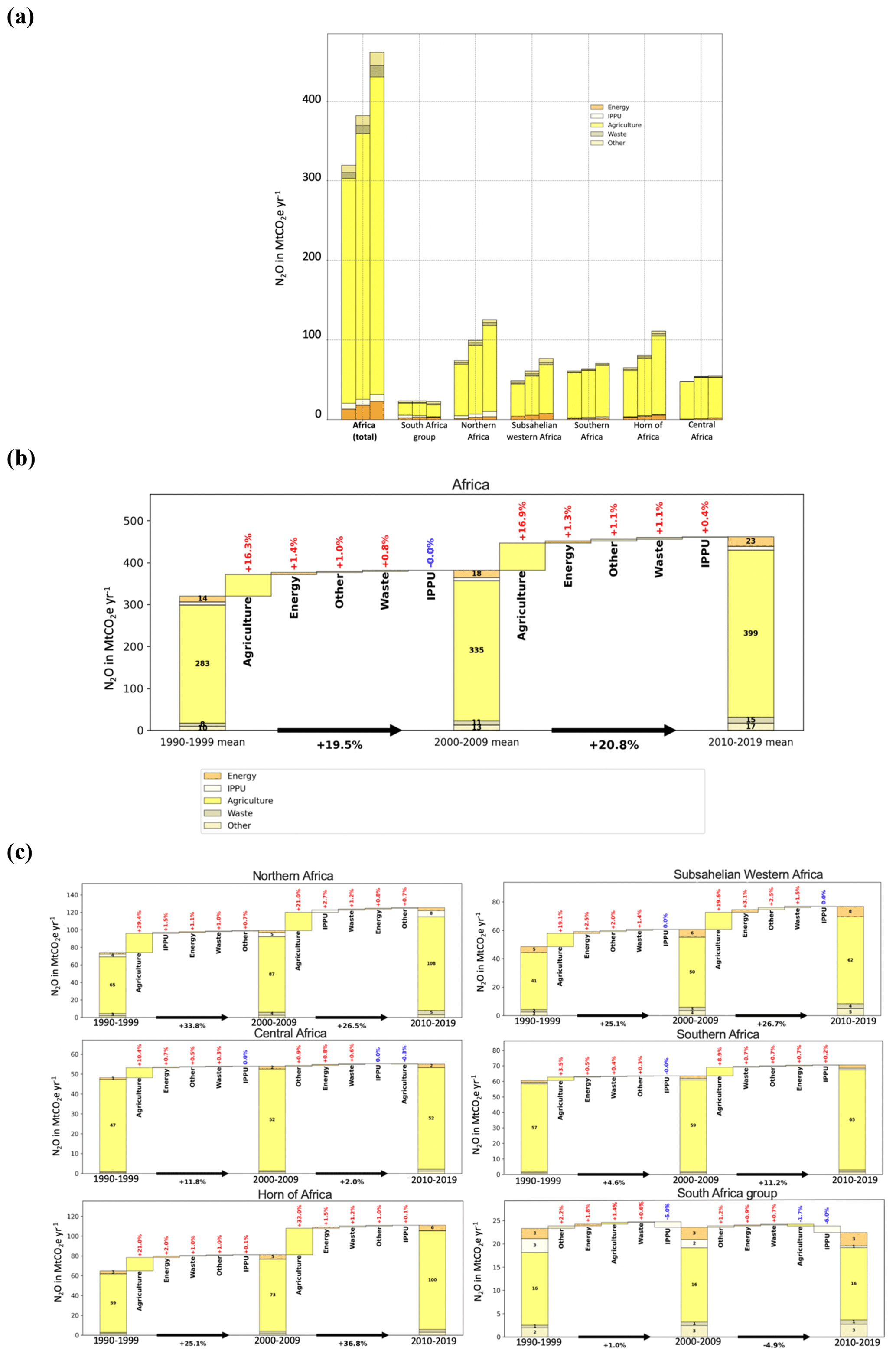
Figure 8 (a) African anthropogenic N₂O emissions (MtCO₂e yr⁻¹) over 3 decades: 1990–1998, 1999–2008 and 2009–2019. Data are from PRIMAP-hist (2021). (b) Contribution of each sector to the change in African N₂O emissions between the last 3 decades. (c) The same for different regions, regrouping several countries. Data are from PRIMAP-hist (2021).

3.4 Results for N₂O emissions

3.4.1 N₂O PRIMAP-hist vs. atmospheric inversions (total flux)

Total and sectoral N₂O anthropogenic emissions (PRIMAP-hist)

Figure 8 presents anthropogenic N₂O emissions from PRIMAP-hist for five sectors (for the country values, see Fig. 4). Over the last 3 decades, the mean African emissions are 378 Mt CO₂ eq. yr⁻¹, 3 times less than CH₄ emissions. The mean decadal N₂O emissions increased from 319 Mt CO₂ eq. yr⁻¹ in 1990–1999 to 382 Mt CO₂ eq. yr⁻¹ in 2000–2009 (+20 %) and further to 431 Mt CO₂ eq. yr⁻¹ in 2010–2018. Over the last 3 decades, the main emitting sector remained Agriculture. The N₂O emission increase also originates from Agriculture, with an increase from 283 to 335 Mt CO₂ eq. yr⁻¹ between 1990–1999 and 2000–2009, i.e., +16.3 % compared to the total emission increase of +19.5 %. The three other sectors show a smaller contribution to the emission increase: Energy (+1.4 %), Other (+1 %) and Waste (+0.8 %). The Industrial Processes and Product Use (IPPU) sector shows no change. Similarly, between 2000–2009 and 2010–2019, the N₂O emission increase also came from the Agriculture sector, with an increase from 335 to 399 Mt CO₂ eq. yr⁻¹ between 1990–1999 and 2000–2009.

The main contributing regions to the continental emissions are northern Africa and the Horn of Africa (Fig. 8a). Between 2000–2009 and 2010–2019, the northern African contribution increased from 99 to 125 Mt CO₂ eq. yr⁻¹ (+27 %). The main sectoral contribution is always Agriculture, which increased in that region from 86 to 107 Mt CO₂ eq. yr⁻¹ (+21 %). Emissions from the second largest emitting region, the Horn of Africa, increased from 81.19 Mt CO₂ eq. yr⁻¹ in 2000–2009 to 111 Mt CO₂ eq. yr⁻¹ in 2010–2019 (+37 %), mainly from Agriculture. In the third most emitting region, sub-Sahelian Africa, emissions increased from 61 Mt CO₂ eq. yr⁻¹ in 2000–2009 to 77 Mt CO₂ eq. yr⁻¹ in 2010–2019 (+27 %), also from Agriculture. The least contributing region to the increase in the total N₂O emissions from 2000–2009 to 2010–2019 is South Africa, which had a very small decrease, mainly from IPPU (−6 %), followed by Agriculture (−2 %). By contrast, there is a slight increase in N₂O emissions for the group of South Africa for the Other (+1 %), Energy (+1 %) and Waste (+1 %) sectors.

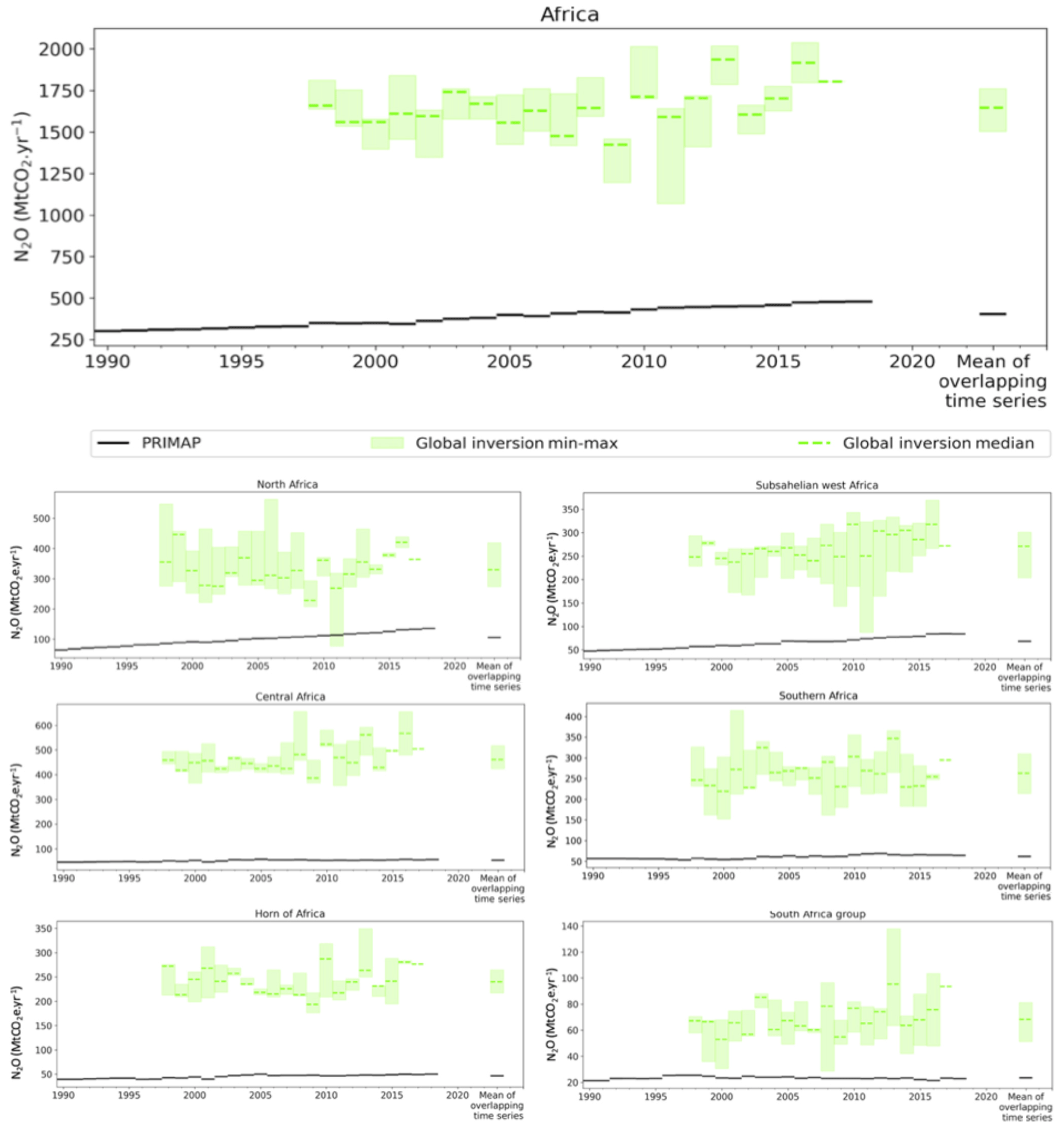
Figure 9 Total N₂O emissions from PRIMAP-hist (MtCO₂e yr⁻¹) (black line) from three GCP atmospheric inversions for the entire African continent and for six African subregions. The green line is the median of the three inversions, and the light green areas show the maximum–minimum range.

Figure 9 compares N₂O emissions from PRIMAP-hist and the inversions. For all of Africa, the mean of inversion emissions over the overlapping time period 1998–2017 is ${\mathrm{1647}}_{\mathrm{1502}}^{\mathrm{1760}}$ Mt CO₂ eq. yr⁻¹, much larger than the PRIMAP-hist estimate of 360 Mt CO₂ eq. yr⁻¹. According to PRIMAP-hist, the total African emissions increased by 28 % between 1998 and 2017, while the trend of emissions from the inversions is 16±8 %. At the regional scale, the emissions from the inversions ranked in decreasing order are central Africa (${\mathrm{461}}_{\mathrm{424}}^{\mathrm{517}}$ Mt CO₂ eq. yr⁻¹ Mt CO₂ eq. yr⁻¹) > northern Africa (${\mathrm{330}}_{\mathrm{274}}^{\mathrm{419}}$ Mt CO₂ eq. yr⁻¹) > sub-Sahelian western Africa (${\mathrm{271}}_{\mathrm{68}}^{\mathrm{330}}$ Mt CO₂ eq. yr⁻¹) > southern Africa (${\mathrm{263}}_{\mathrm{214}}^{\mathrm{310}}$ Mt CO₂ eq. yr⁻¹ > Horn of Africa ${\mathrm{240}}_{\mathrm{217}}^{\mathrm{265}}$ Mt CO₂ eq. yr⁻¹ > South Africa (${\mathrm{68}}_{\mathrm{51}}^{\mathrm{81}}$ Mt CO₂ eq. yr⁻¹). According to PRIMAP-hist, the ranking is northern Africa (106 Mt CO₂ eq. yr⁻¹) > sub-Sahelian western Africa (68 Mt CO₂ eq. yr⁻¹) > southern Africa (62 Mt CO₂ eq. yr⁻¹) > central Africa (54 Mt CO₂ eq. yr⁻¹)> Horn of Africa (46 Mt CO₂ eq. yr⁻¹) > South Africa (24 Mt CO₂ eq. yr⁻¹) (see also Table S13). Emissions from PRIMAP-hist are smaller than the inversions by a factor of 16. This is likely due to the fact that we did not attempt to separate natural and anthropogenic emissions in the inversions. Other studies (Deng et al., 2022; Petrescu et al., 2021, in Europe) showed that, even after subtracting N₂O natural estimates, the inversions always point to higher estimates than the BU methods.

4 Discussion: uncertainties, comparison between BU and TD methods as well as synthesis for the three main GHGs

4.1 Uncertainties specific to DGVMs and inversions for LULUCF CO₂

In Fig. 5, we showed important disagreements among models regarding LULUCF CO₂ on whether Africa has been a small source over the last 20 years (as shown by inversions) or a net sink (as shown by DGVMs and UNFCCC except with the Grassi correction). There is also more interannual variability in the DGVMs results, mainly from climate variability, which is absent from UNFCCC as inventories provide only decadal smoothed flux estimates. The larger sink in the DGVMs compared to the corrected UNFCCC estimates using the method of Grassi et al. (2022) may be due to the fact that non-Annex I UNFCCC estimates generally do not include dead biomass or harvested wood products. If forest biomass is estimated by a stock change approach, therefore, changes in living biomass due to transfer to dead biomass and harvested wood products will be considered emitted in that year, while in the DGVMs it will decay more slowly over time. Another difference is the treatment of land use change emissions based on historical global land use change maps for the DGVMs, which can significantly differ from national land use datasets. On the other hand, DGVMs do not represent forestry and may underestimate sinks in intensively managed young forests. DGVMs do not distinguish between unmanaged and managed lands, while UNFCCC inventories only account for managed land but include conservation areas and indigenous territories. Grassi et al. (2022) showed that the difference between the global UNFCCC sink (1100 Mt CO₂ yr⁻¹) and the global land carbon sink (4767 Mt CO₂ eq. yr⁻¹) must be explained by the contribution of non-managed lands. However, in the case of Africa, it was not possible to extract from UNFCCC reports the national areas of unmanaged land, and we also had to look at the UNFCCC Technical Assessment Reports (TARs) as well as REDD+ reports to extract information. Methods of assessment have not been fully standardized since 1990, and they differ depending on the countries analyzed and on the emission categories considered. In this context, when comparing UNFCCC estimates with data from DGVMs and inversion models, different layers of aggregated uncertainties affect the analysis (Deng et al., 2022; Petrescu et al., 2021; Grassi et al., 2018). The fact that LULUCF CO₂ fluxes have the greatest uncertainties is true globally.

4.2 Differences and sources of uncertainties between BU and TD CH₄ emissions

The methodology used to remove natural CH₄ emissions from inversions is key to comparing them with BU estimates of anthropogenic emissions only. In this paper, we used a separation based on the natural emissions solved by each inversion (Sect. 2.3, Method 1). Using an alternative method from Deng et al. (2022) based on natural emissions from the median of all the inversions gives smaller anthropogenic emissions than PRIMAP-hist (Fig. S10).

4.3 Differences and sources of uncertainties between BU and TD N₂O emissions

For N₂O emissions, discrepancies between inventories and inversions are very high, especially for the group of central African countries where the vegetation covers an important land area with likely high natural N₂O (Deng et al., 2022). We can suppose that, more broadly for all African groups, the lack of accounting for natural emissions is the main reason why PRIMAP-hist estimates are much smaller than those of inversions. All the African countries used Tier 1 emission factors and include only direct N₂O emissions. The study by Deng et al. (2022) underlined that indirect anthropogenic emissions notably coming from “atmospheric nitrogen deposition and leaching from anthropogenic nitrogen additions to aquifers and inland water are usually not reported by non-Annex I countries” and that this underreported source of anthropogenic emissions tends to represent about 5 % to 10 % of anthropogenic N₂O. According to Deng et al. (2022), the global situation from inversions for the main emitters is similarly affected by the potential contribution of natural sources as well, which is difficult to estimate and separate. Figure 11 from Deng et al. (2022) shows that, even when removing “intact/non-managed lands” from inversions, in many countries, especially tropical countries, the inversions give a systematically much higher anthropogenic level of N₂O than the inventories, suggesting that there are either missing anthropogenic sources or some “natural” sources (e.g., conservation areas) in managed lands that are underestimated by inventories.

4.4 Synthesis of the steps for assessing net GHG trends over Africa

Here, we propose a first step towards the elaboration of what could become a more systematic method for a scientific benchmark of non-Annex I national inventories: (1) correct outliers, (2) check the plausibility of estimates, (3) have an independent evaluation of inventory data by experts, (4) compare UNFCCC data corrected thanks to expert judgment and other BU and TD methods, (5) compute the mean of all the BU and TD methods, (6) compute “best-fitted BU values” (meaning best-fitted BU values excluding uncorrected UNFCCC data) and “TD values” (meaning “best-fitted TD values” without considering N₂O inversions replaced with PRIMAP-hist values), and (7) identify ranking anomalies.

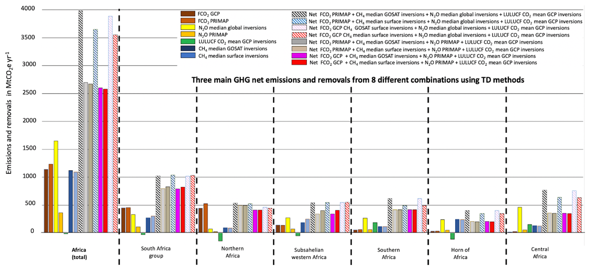
Figure 10 Synthesis for the three main GHGs with net African budget computation by all the TD methods for Africa as a whole and for six subgroups of African countries across overlapping time series (2001–2017). Following the atmospheric convention, positive numbers represent an emission into the atmosphere and negative values represent a sink. The CO₂ emissions and sinks from LULUCF are represented in green; they are taken from the GCP 2020 dataset (MtCO₂e yr⁻¹).

4.5 Net GHG budget from inversions

Figure 10 shows different combinations of inversion GHG budgets and individual gas contributions.

For the African total, the mean net GHG budget from the inversions where N₂O inversions are replaced by PRIMAP-hist is ${\mathrm{2638}}_{\mathrm{1761}}^{\mathrm{5873}}$ Mt CO₂ eq. yr⁻¹. The regional GHG budgets in decreasing order are northern Africa (${\mathrm{810}}_{\mathrm{279}}^{\mathrm{1170}}$ Mt CO₂ eq. yr⁻¹) > South African group (${\mathrm{452}}_{\mathrm{161}}^{\mathrm{751}}$ Mt CO₂ eq. yr⁻¹) > southern Africa $({\mathrm{416}}_{-\mathrm{334}}^{\mathrm{1465}}$ Mt CO₂ eq. yr⁻¹) > sub-Sahelian western Africa (${\mathrm{373}}_{\mathrm{36}}^{\mathrm{1051}}$ Mt CO₂ eq. yr⁻¹) > central Africa (${\mathrm{352}}_{-\mathrm{1133}}^{\mathrm{1592}}$ Mt CO₂ eq. yr⁻¹) > Horn of Africa $({\mathrm{204}}_{-\mathrm{456}}^{\mathrm{873}}$ Mt CO₂ eq. yr⁻¹) (Table S17). The mean net of inversions including N₂O inversions is substantially higher, ${\mathrm{3879}}_{\mathrm{1320}}^{\mathrm{7341}}$ Mt CO₂ eq. yr⁻¹. The regional GHG budgets in decreasing order are northern Africa $({\mathrm{1034}}_{\mathrm{600}}^{\mathrm{1475}}$ Mt CO₂ eq. yr⁻¹) > central Africa (${\mathrm{759}}_{-\mathrm{763}}^{\mathrm{2054}}$ Mt CO₂ eq. yr⁻¹) > southern Africa (${\mathrm{616}}_{-\mathrm{262}}^{\mathrm{1713}}$ Mt CO₂ eq. yr⁻¹) > sub-Sahelian western Africa (${\mathrm{576}}_{-\mathrm{61}}^{\mathrm{1313}}$ Mt CO₂ eq. yr⁻¹) > South African group $({\mathrm{496}}_{\mathrm{138}}^{\mathrm{814}}$ Mt CO₂ eq. yr⁻¹) (Table S17).

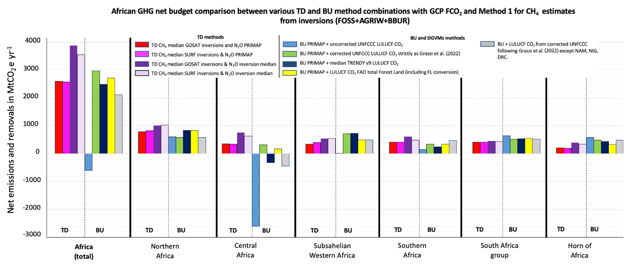
Figure 11 Synthesis for the three main GHG net African budgets from the TD and BU methods, using Method 1 for separating anthropogenic CH₄ emissions from inversions (FOSS + AGRIW + BBUR) during 2001–2017. FCO₂ data are from GCP. The N₂O is from the global inversions and from PRIMAP-hist. For the TD method, anthropogenic CH₄ from both GOSAT and surface inversions is used, and LULUCF is from GCP inversions only. For the BU methods, anthropogenic CH₄ and N₂O from PRIMAP are used and with five different methods for assessing LULUCF CO₂: from uncorrected UNFCCC data; from corrected UNFCCC data according to Grassi et al. (2022); from corrected UNFCCC except for Namibia, Nigeria and the DRC; from TRENDY version 9; and from the FAO FL, including FL conversions. Following the atmospheric convention, positive numbers represent an emission into the atmosphere and the negative values represent a sink (MtCO₂e).

4.6 Comparison between the BU and TD methods

Figure 11 shows the GHG budgets from all the combinations of the BU and TD methods. The mean of all the methods after filtering outliers (Grassi et al. (2022) and UNFCCC corrections using PRIMAP instead of inversions for N₂O) is ${\mathrm{2630}}_{\mathrm{1974}}^{\mathrm{4557}}$ Mt CO₂ eq. yr⁻¹, which represents only 7.3 % of global FCO₂ emissions. The mean of all the estimates points to a source in the six African regions ranked in decreasing order as northern Africa $({\mathrm{761}}_{\mathrm{460}}^{\mathrm{988}}$ Mt CO₂ eq. yr${}^{-\mathrm{1}}({\mathrm{513}}_{\mathrm{161}}^{\mathrm{702}}$ Mt CO₂ eq. yr⁻¹) > Horn of Africa $({\mathrm{318}}_{-\mathrm{80}}^{\mathrm{699}}$ Mt CO₂ eq. yr⁻¹) > sub-Sahelian western Africa (${\mathrm{492}}_{\mathrm{286}}^{\mathrm{913}}$ Mt CO₂ eq. yr⁻¹) > southern Africa $({\mathrm{354}}_{-\mathrm{78}}^{\mathrm{998}}$ Mt CO₂ eq. yr⁻¹) > central Africa $({\mathrm{143}}_{-\mathrm{670}}^{\mathrm{882}}$ Mt CO₂ eq. yr⁻¹).

We initially did not make any assumption regarding which approach is “better” between the TD and BU methods, as this actually depends on the considered gas, sector and spatial scales. Comparability between TD and BU results is not completely obvious either, as they do not represent the same processes (the example of LULUCF CO₂ for DGVMs is explained in Sect. 3.1). For N₂O specifically, we highlighted in Sect. 3.3 the large uncertainty in the TD estimates, underlining the importance of separating natural N₂O emissions from total estimates in order to deliver appropriate anthropogenic assessments thanks to the inversions.

We showed in the results of this paper that inversions in general tend to have larger uncertainties than the inventories as well as large differences in terms of minima or maxima and at the annual scale, even among similar typologies of the methods. However, at the decadal scale, they show reliable overall trends (with good matches among the median values of various estimates in the overlapping time period), especially at the spatial scale of groups of countries and of a continent. Under such conditions, TD estimates help identify or confirm outliers or large uncertainties in inventories that may occur, especially for non-Annex I countries like in Africa.

Inversions therefore cannot be a substitute, but they are rather a complement to check trend consistencies in inventories and to help identify and correct the main outliers. That is why we chose BU estimates to deliver a final budget over Africa (with CO₂ LULUCF corrections) as synthesis figures (see Figs. 12 and 13 in the next paragraph). The possibilities for reducing the gap BU and TD estimates are the following. (1) For inversions, have a coarser network of surface stations and coarser spatial resolutions. (2) For DGVMs, see Sect. 3.1. (3) For national UNFCCC inventories, have regularly updated activity data, use country-specific emission data and include indirect emissions, which is not the case to date for African countries, and use expert judgment to correct outliers as done by Grassi et al. (2022) and in this study for CO₂ LULUCF emissions.

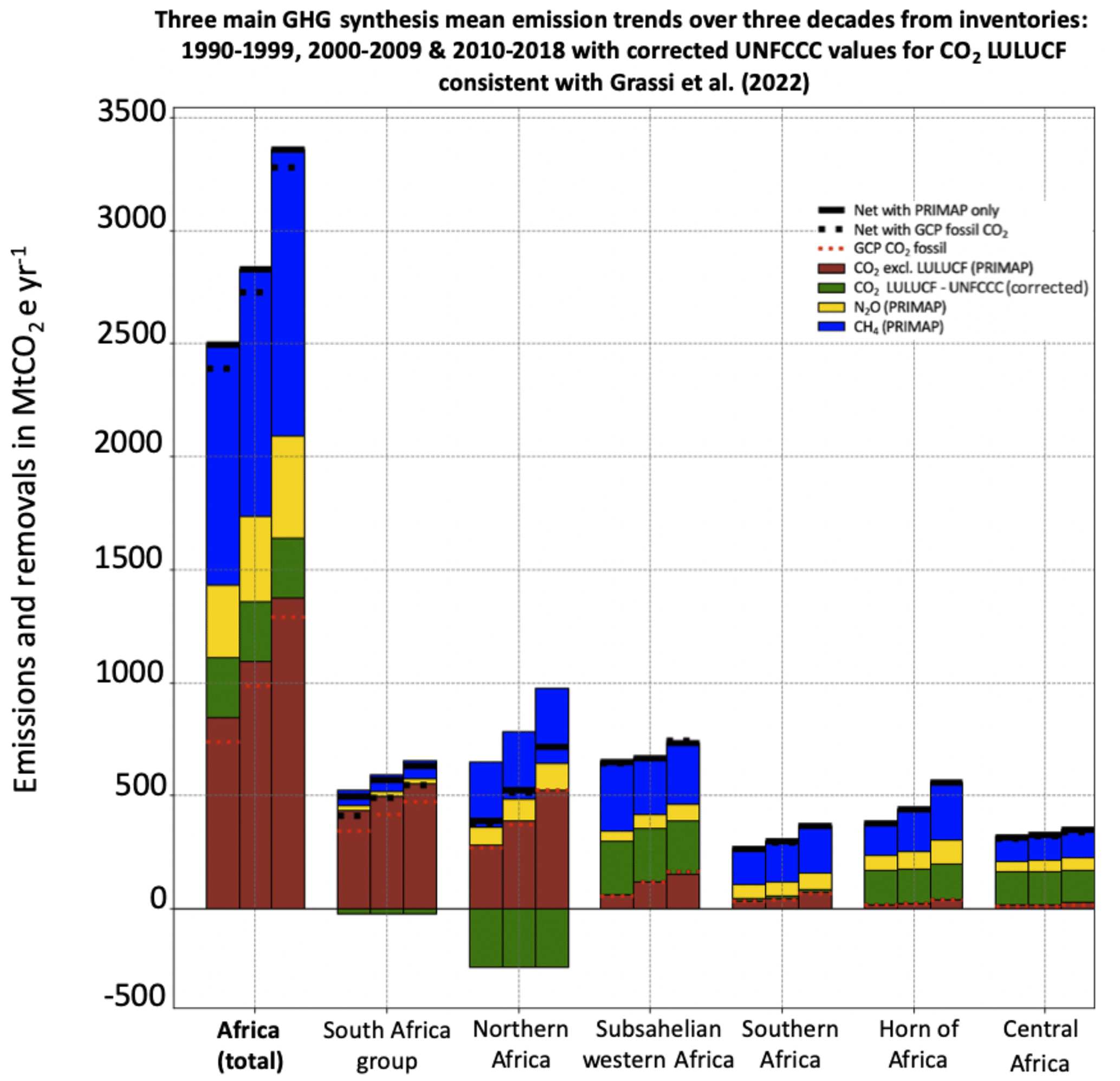
Figure 12 Synthesis for the three main GHGs from the inventories (after UNFCCC LULUCF CO₂ corrections consistent with Grassi et al., 2022) for the three main GHGs with net African budget computation by BU inventories for Africa as a whole and for six subgroups of African countries across 3 different decades (1990–1999, 2000–2010 and 2010–2018) using data and corrections from country inventories. Following the atmospheric convention, positive numbers represent an emission into the atmosphere and negative values represent a sink. Black horizontal lines represent a net flux resulting from the addition of the three main GHGs using PRIMAP-hist only, and dashed black horizontal lines also represent the net flux resulting from the addition of the three main GHGs but using the GCP dataset for FCO₂. Dashed red lines represent the fluxes from GCP FCO₂ available in the most recent GCP paper to compare them with PRIMAP-hist results, which are represented with the brown bar plots. The N₂O and CH₄ fluxes from PRIMAP-hist are represented with yellow and blue bars, respectively. CO₂ emissions and sinks from LULUCF are represented in green; they are taken from NC or BUR UNFCCC datasets with corrections applied (MtCO₂e yr⁻¹).

4.7 Net GHG budget from BU estimates

Figure 12 shows the budget for the three GHGs from UNFCCC data with LULUCF data corrected using the second approach. There is a clear increase in African total GHG emissions during the last 3 decades. The differences between the BU datasets are mainly due to different sectoral allocations. However, the trends are consistent and comparable, and differences among inventories tend to be less for the most recent decade.

Table 4 Mean net total African and regional group emissions and removals from BU methods using either GCP or PRIMAP-hist for FCO₂ over 2001–2017 (MtCO₂e yr⁻¹).

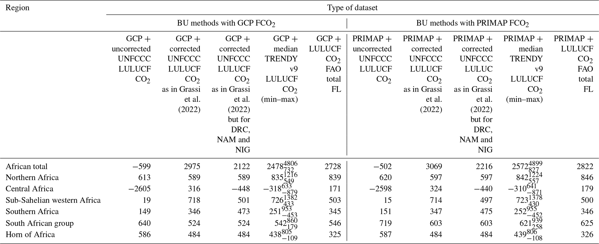
At the country level, a small number of countries showed an increasing difference between PRIMAP-hist and GCP estimates of fossil CO₂ emissions over time, but they are small FCO₂ emitters. The differences may also be partly explained by changes in accounting methods as mentioned in Gütschow et al. (2016). The biggest discrepancies are noticeable for Mali (64 %), Cameroon (−62 %) and the DRC (−38 %), but those three countries are not major FCO₂ emitters (Fig. 4a–b).

Table 4 shows the differences in the net African budget from various BU methods using GCP or PRIMAP-hist for FCO₂ over 2001–2017 that are also illustrated in Fig. 11.

4.7.1 BU LULUCF budget from UNFCCC corrected by Grassi et al. (2022)

Over 2001–2017, the net BU GHG budget is 2975 Mt CO₂ eq. yr⁻¹. Regionally, the ranking in decreasing order is sub-Sahelian western Africa (718 Mt CO₂ eq. yr⁻¹) > northern Africa (588 Mt CO₂ eq. yr⁻¹) > South African group (524 Mt CO₂ eq. yr⁻¹) > Horn of Africa (484 Mt CO₂ eq. yr⁻¹) > southern Africa (346 Mt CO₂ eq. yr⁻¹) > central Africa (316 Mt CO₂ eq. yr⁻¹).

4.7.2 BU LULUCF budget CO₂ from the FAO

The BU budget from the FAO data is 2728 Mt CO₂ eq. yr⁻¹, 8 % less than above. The ranking of the regions in decreasing order is northern Africa (838 Mt CO₂ eq. yr⁻¹) > South African group (546 Mt CO₂ eq. yr⁻¹) > sub-Sahelian western Africa (503 Mt CO₂ eq. yr⁻¹) > southern Africa (345 Mt CO₂ eq. yr⁻¹) > Horn of Africa (325 Mt CO₂ eq. yr⁻¹) > central Africa (171 Mt CO₂ eq. yr⁻¹).

4.7.3 BU LULUCF budget from DGVMs

The net GHG budget for Africa is ${\mathrm{2478}}_{\mathrm{733}}^{\mathrm{4806}}$ Mt CO₂ eq. yr⁻¹, 9 % less than with the FAO. The ranking of the regions in decreasing order is northern Africa (${\mathrm{835}}_{\mathrm{549}}^{\mathrm{1216}}$ Mt CO₂ eq. yr⁻¹) > sub-Sahelian western Africa (${\mathrm{726}}_{\mathrm{433}}^{\mathrm{1382}}$ Mt CO₂ eq. yr⁻¹) > South Africa (${\mathrm{542}}_{\mathrm{179}}^{\mathrm{859}}$ Mt CO₂ eq. yr⁻¹) > Horn of Africa (${\mathrm{438}}_{-\mathrm{109}}^{\mathrm{805}}$ Mt CO₂ eq. yr⁻¹) > southern Africa (${\mathrm{251}}_{-\mathrm{453}}^{\mathrm{953}}$ Mt CO₂ eq. yr⁻¹ > central Africa ($-{\mathrm{318}}_{-\mathrm{879}}^{\mathrm{633}}$ Mt CO₂ eq. yr⁻¹).

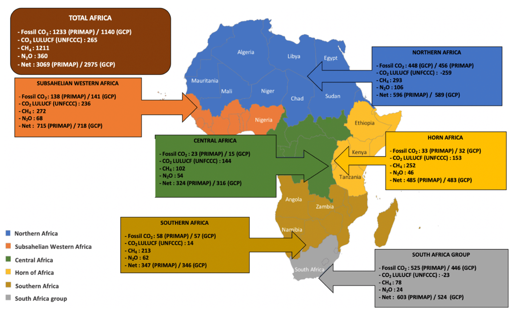
Figure 13 The 2001–2018 emissions (MtCO₂e yr⁻¹) for fossil CO₂ (GCP and PRIMAP-hist), LULUCF CO₂ (corrected UNFCCC data consistent with Grassi et al., 2022), CH₄ (PRIMAP-hist) and N₂O (PRIMAP-hist) for Africa and for the six regions.

For information, in the Supplement, Figs. S13 and S14 illustrate the differences (MtCO₂e and percentage) for CH₄, N₂O and the total net GHG budget that would result from the use of AR6 GWP100 compared to AR4 GWP100 currently in use by UNFCCC non-Annex I countries, for the six African regions considered in Fig. 13 as well as for the African total. The net difference in the total African budget for the use of GWP100 AR6 instead of AR4 is +4.6 %, which means a relatively small increasing impact on the net budget, with a prevailing effect of the slight increase in CH₄ GWP100 in AR6 as compared to AR4 over the strong decrease in N₂O GWP-100. The two African regions that are the most impacted in terms of net budget are the southern countries (+7.2 %) and the Horn of Africa (+6.3 %). The least impacted region in terms of overall net budget with an updated AR6 GWP-100 for CH₄ and N₂O is South Africa (+1.7 %).

5 Data availability

The datasets from the three main greenhouse gases used in this paper (CO₂, CH₄ and N₂O) from the various BU inventories, TD inversions and DGVMs over Africa will be made publicly available. This database is available from Zenodo at https://doi.org/10.5281/zenodo.7347077 (Mostefaoui et al., 2022).

This dataset contains 32 data files.

• CO₂ inversions (annual flux for LULUCF CO₂)

• African CO₂ TD inversions GCB2020 1990–2019: annual CO₂ flux from GCB inversion models

• African CO₂ lateral flux 2001–2019: annual CO₂ lateral flux including river transport, crop and wood product trade

• African CO₂ TRENDY version 9 1990–2019: annual CO₂ flux from 14 DGVMs

• FAO 1990–2019: annual emissions and removals from the FAO dataset

• Inventory IPCC 1990–2019: annual flux from inventory data collected from UNFCCC national inventories in the IPCC categories

• CH₄ inversions for 2000–2017 (annual flux)

• African CH₄ global inversion 2000–2017: CH₄ flux over 2000–2017 from 11 surface inversions and 11 satellite inversion models from four sectors. “Fossil” refers to emissions from the fossil sector. “Agriculture” and “Waste” refer to emissions from both the agriculture and waste sectors. “Biomass burning” refers to emissions from biomass burning.

• GFED version 4 1997–2016: wildfire emissions from GFED version 4

• N₂O inversions for 1998–2017 (annual flux)

• N₂O PYVAR 1998–2017: total N₂O emissions from PyVAR inversions

• N₂O TOMCAT-INVICAT 1998–2015: total N₂O emissions from the TOMCAT-INVICAT model

• N₂O MIROC4-ACTM 1998–2016: total N₂O emissions from the MIROC4-ACTM model

Data used in this study are also included in the Supplement (for example, from FAO data) and on public websites (CDIAC, PRIMAP-hist, World Bank data). Any other data that support the findings of this study are available from the corresponding author upon request.

6 Summary, concluding remarks and perspectives

Africa is a large continent with 56 countries, and some of the countries are major GHG emitters. Because of its rapidly growing population and high industrial potential, Africa has a critical geography regarding climate change mitigation and adaptation policy. Depending on the emission pathways, Africa, which is already a big emitting region, is expected to represent at least a bit more than 10 % of the global share by 2050, which could become as high as 18 % of global emissions by 2050 (van der Zwaan et al., 2018).

This paper presents both a continental view and a detailed analysis of the three main GHG trends during the last 30 years across this continent as a whole and across relevant groups of countries given the inversions' resolutions and also considering the countries' details. Thanks to the comparison of different methods and datasets, the uncertainty about the net emissions and removals of GHGs decreases. The interest in studying Africa is high not only from a scientific point of view but also from a climate-policy perspective, as under the UNFCCC principle of “common but differentiated responsibility” about global warming, the credibility of the PA lies in the effective participation and inclusiveness of all the parties, including non-Annex I countries. Our effort in comparing BU datasets and inversions and analyzing differences for African GHG emissions and removal assessment by looking at trends since 1990 will also be useful for future updates on a regular basis within the 2023 GST perspective.

At the scale of Africa, there is a rapid increase in FCO₂ emissions that has roughly doubled since 1990. This increase is dominated by coal emissions for the decade 1990–1998 compared to 1999–2008 (+9 %) and by oil for the decade 1999–2008 compared to the decade 2008–2017 (+16 %). As for CO₂ LULUCF, we found that BU estimates are characterized by important annual fluctuations, as opposed to periodic national inventory assessments, and the reconciliation between the sectoral classification for anthropogenic estimates between TD and BU has to be done “manually” and is not uniform to date, which does not facilitate the comparability of those different approaches. There are also differences between GCP inversions for CO₂ due to the fact that choices of model transport may differ among models, because prior fluxes can also differ between modeling teams and because the African GHG observation network is characterized by few stations and relatively scarce data. The lack of integration of CO₂ lateral anthropogenic and river fluxes is also an issue to be taken into account when trying to compare BU and TD methods (Ciais et al., 2022), and in the present study we did integrate those lateral fluxes. Anthropogenic CH₄ from PRIMAP-hist estimates indicates that, of the total African emission increase from 1064 to 1116 Mt CO₂ eq. yr⁻¹ between 1990–2000 and 2001–2009 (+5 %), only two sectors contributed: Agriculture, in a dominant way (+8 %), and Waste (+5 %). Energy contributes to emission decrease (−8 %), which is however too small to offset other sectors' CH₄ emissions that represent a net increase. The main regional contributions come from northern Africa and from the Agriculture sector (+12 %). Over the same period, the least contributing emitter is the group of South Africa (+12 %), with only one decreasing emission sector: Agriculture (−1 %). The mean 2001–2009 emissions increased by +15 % over 2010–2018, with contributions from all the sectors except for IPPU. This increase is dominated by Agriculture (+8 %) and Waste (+6 %). For 2010–2018, the two main contributing regions for CH₄ emissions are northern Africa and sub-Sahelian western Africa, Agriculture being the dominant emitting sector. From inversions, after withdrawing natural emissions and wildfires using the GFED dataset from the total CH₄ emissions, median values are almost always below PRIMAP-hist estimates. CH₄ natural emissions have an important impact in Africa, especially in the central African region as well as in the southern countries. N₂O TD estimates are always higher than the ones from PRIMAP-hist, underlining the importance of separating natural N₂O emissions from total estimates in order to deliver appropriate anthropogenic assessments thanks to the inversions.

To compute a net budget for the three main GHG emissions and removals, and for comparability, we used the Mt CO₂ eq. yr⁻¹ metric and the latest IPCC report-recommended GWP. The choice of a constructed GWP metric, however, creates additional associated uncertainties, notably due to the selected time horizon. By computing the mean of methods excluding uncorrected UNFCCC and N₂O inversion data from 20 different ways of assessing GHG emissions and removals in Africa, we found that the most recent net budget from the three main GHGs in Africa is a source of ${\mathrm{2630}}_{\mathrm{1974}}^{\mathrm{4557}}$ Mt CO₂ eq. yr⁻¹.

Our assessment of African GHG emission trends over 30 years through different methods can enable comparisons of ex post and ex ante pledges of the PA, whose baseline year is often 1990. However, given the global geopolitics to date characterized by the prevailing principle of national sovereignty, a scientific assessment of GHGs can only work as a supporting tool (Janssens-Maenhout et al., 2020) and cannot be directly policy-prescriptive. We note a relatively good match among the various types of estimates in terms of overall trends, especially at a regional level and on a decadal basis, but large differences exist in terms of minima and maxima and at the annual scale, even among similar typologies of the methods (TD or BU). The large discrepancies are a scientific limit to the possibility of precise verification of the African country-reported emissions, but they are good enough to indicate trends. To compute a net from the three main GHGs, no purely TD method is available due to the necessity to replace N₂O inversion data with BU data. An original result of this study is that we proposed at a small scale what may become a systematic formalized methodological protocol for independent verification of a net estimate using country-reported data to be possibly implemented at the UNFCCC secretariat scale in a centralized way. The African GHG increasing trend is not in line with the mitigation aims of the PA towards net-zero globally. Research teams focusing on inversion methods (Nickless et al., 2020) underline that uncertainties should not be above 15 % in order to deliver a reasonable verification support capacity. A major source of complexity for the evaluation of the respect of the Paris Agreement comes from the fact that national pledges generally fall below the discrepancies between different scientific independent estimates. This calls for investments not only in improvements of atmospheric measurement devices, but also in research efforts for standardizing verification methods. At the policy level, the extrapolation of this study to the climate policy field could also serve as a compelling argument for the creation of a global dedicated “climate inspection task force” of the UNFCCC.