The 2023 National Offshore Wind data set (NOW-23)

This article introduces the 2023 National Offshore Wind data set (NOW-23), which offers the latest wind resource information for offshore regions in the United States. NOW-23 supersedes, for its offshore component, the Wind Integration National Dataset (WIND) Toolkit, which was published a decade ago and is currently a primary resource for wind resource assessments and grid integration studies in the contiguous United States. By incorporating advancements in the Weather Research and Forecasting (WRF) model, NOW-23 delivers an updated and cutting-edge product to stakeholders. In this article, we present the new data set which underwent regional tuning and performance validation against available observations and has data available from 2000 through, depending on the region, 2019–2022. We also provide a summary of the uncertainty quantification in NOW-23, along with NOW-WAKES, a 1-year post-construction data set that quantifies expected offshore wake effects in the US Mid-Atlantic lease areas. Stakeholders can access the NOW-23 data set at https://doi.org/10.25984/1821404 (Bodini et al., 2020).

1 Introduction

In this article, we present the work done to create a state-of-the-art wind resource data set for all United States offshore regions (except for Alaska), called the 2023 National Offshore Wind data set (NOW-23). This work has been performed by the National Renewable Energy Laboratory (NREL) and its partners, the University of Colorado, Boulder, and Veer Renewables.

In 2015, NREL produced the Wind Integration National Dataset (WIND) Toolkit (Draxl et al., 2015), a 7-year wind resource data set (2007–2013) covering the contiguous United States. The WIND Toolkit was built using the Weather Research and Forecasting (WRF) mesoscale numerical weather prediction (NWP) model (Skamarock et al., 2021) and provided modeled variables up to 200 m above the surface. Since its creation, the WIND Toolkit has become one of the most comprehensive and commonly used data sets for wind resource assessment and grid integration studies in the United States, owing to the fact it has been publicly available at no cost through Amazon Web Services. A wide variety of stakeholders, ranging from wind energy developers and consultants, utilities, government organizations, and academic and research institutions, have taken advantage of the WIND Toolkit to foster wind energy development across the United States.

Since the release of the WIND Toolkit, extensive research in the field of NWP models has been completed, and many advancements have been proposed and tested by the global atmospheric science community. Several field campaigns (e.g., Wilczak et al., 2015; Shaw et al., 2019; Fernando et al., 2019) have been completed to collect observations useful to validate and improve the capabilities of the WRF model. Growing research has assessed the sensitivity in the modeled wind resource to different model inputs and parameterizations (e.g., Hahmann et al., 2020). Also, new state-of-the-art reanalysis products (namely ERA5; Hersbach et al., 2020) have been released and can now be used as boundary conditions to feed the WRF model. Finally, a broader scientific consensus agrees that data sets of at least 20 years are needed for a robust quantification of the long-term wind resource at the site of interest.

Given the extensive success of the WIND Toolkit, NREL and its partners are committed to ensuring that the latest advancements in the atmospheric modeling community are provided to stakeholders. As such, a next-generation product to replace the WIND Toolkit is needed to ensure that the most accurate wind resource data are given to the US wind energy community. Given the current and expected future sparsity of offshore hub height observations, a national state-of-the-art mesoscale modeled wind resource data set represents an even more critical need to support the breadth of offshore wind energy analyses and stakeholders that rely on such data.

Here, we present NOW-23, a validated national offshore wind resource data set for the United States. The main final product of this research effort is a WRF-based atlas of the offshore wind resource for all US offshore waters, covering at least 20 years, which is made available at no cost to the public, with data at 5 min temporal resolution, 2 km horizontal resolution, and up to 500 m above the surface. In Sect. 2, we present the general modeling approach used to develop the NOW-23 data set. Sections 3 through 10 describe the NOW-23 data set in each modeled offshore region. Section 11 describes our uncertainty quantification efforts. Section 12 introduces NOW-WAKES, a post-construction data set for the Mid-Atlantic domain. In Sect. 13, we provide instructions on how to access the NOW-23 data set, followed by our main conclusions. In the Appendix, we provide additional analyses on the seasonal and diurnal variability in the modeled wind resource, the variability in the mean wind speed at overlapping boundaries of neighboring regional domains, and a comparison of the mean wind speed predictions with what was modeled by the previous-generation WIND Toolkit.

2 Description of the WRF model simulations and general validation approach

To create the NOW-23 data set, we adopt a regional approach. For each offshore region, we perform a separate numerical simulation, whose setup is selected (in most regions) through validation against available observations, so that the model can be customized to account for regionally unique wind resource phenomena. Figure 1 shows the eight regional domains of the NOW-23 data set. We note that WRF model domains have a rectangular shape. However, to limit the storage requirements for the NOW-23 data files, most of the regional data sets are masked (after the WRF model simulations are done) based on the extension of the exclusive economic zone (EEZ), which is the area in which a country has jurisdiction over natural resources, including wind, roughly at 212 nmi from the coast.

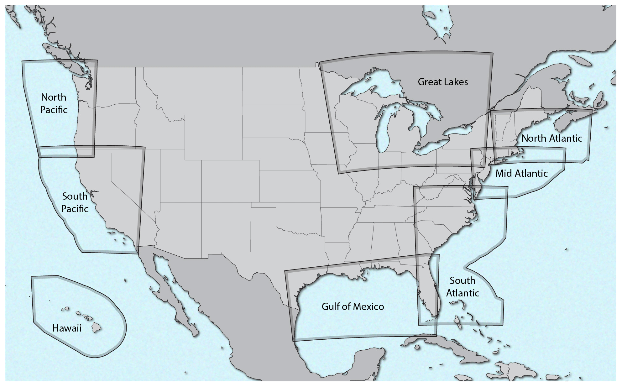
Figure 1 Map of the regional WRF model domains used to build the NOW-23 data sets masked at the limit of the exclusive economic zone of the countries with jurisdiction on the offshore regions being considered.

Table 1 summarizes the main attributes for the WRF model simulations used to build NOW-23 and compares them with those of the older WIND Toolkit. We run the simulations in 1-month segments and then concatenate them at each grid cell in the post-processing phase. In doing so, we consider a spin-up period of 2 d (for example, the May 2015 run actually starts on 29 April 2015) to let the model stabilize from the initial conditions imposed to the WRF model. The choice of using 1-month segments is dictated by the need to have a limited number of restart periods for grid applications, as every restart might create false ramps, and by the desire to reduce the overall time needed to run the simulations, given the parallel computing capabilities offered by NREL's supercomputer where the simulations are performed. As will be detailed in later sections, we do not observe degraded performance with time in each calendar month. The choice of the 5 min temporal resolution is also to accommodate needs the of the grid integration community.

Table 1 Main attributes of the NOW-23 data set compared to those used in the older WIND Toolkit. Attributes in bold are the result of a region-specific sensitivity analysis in NOW-23.

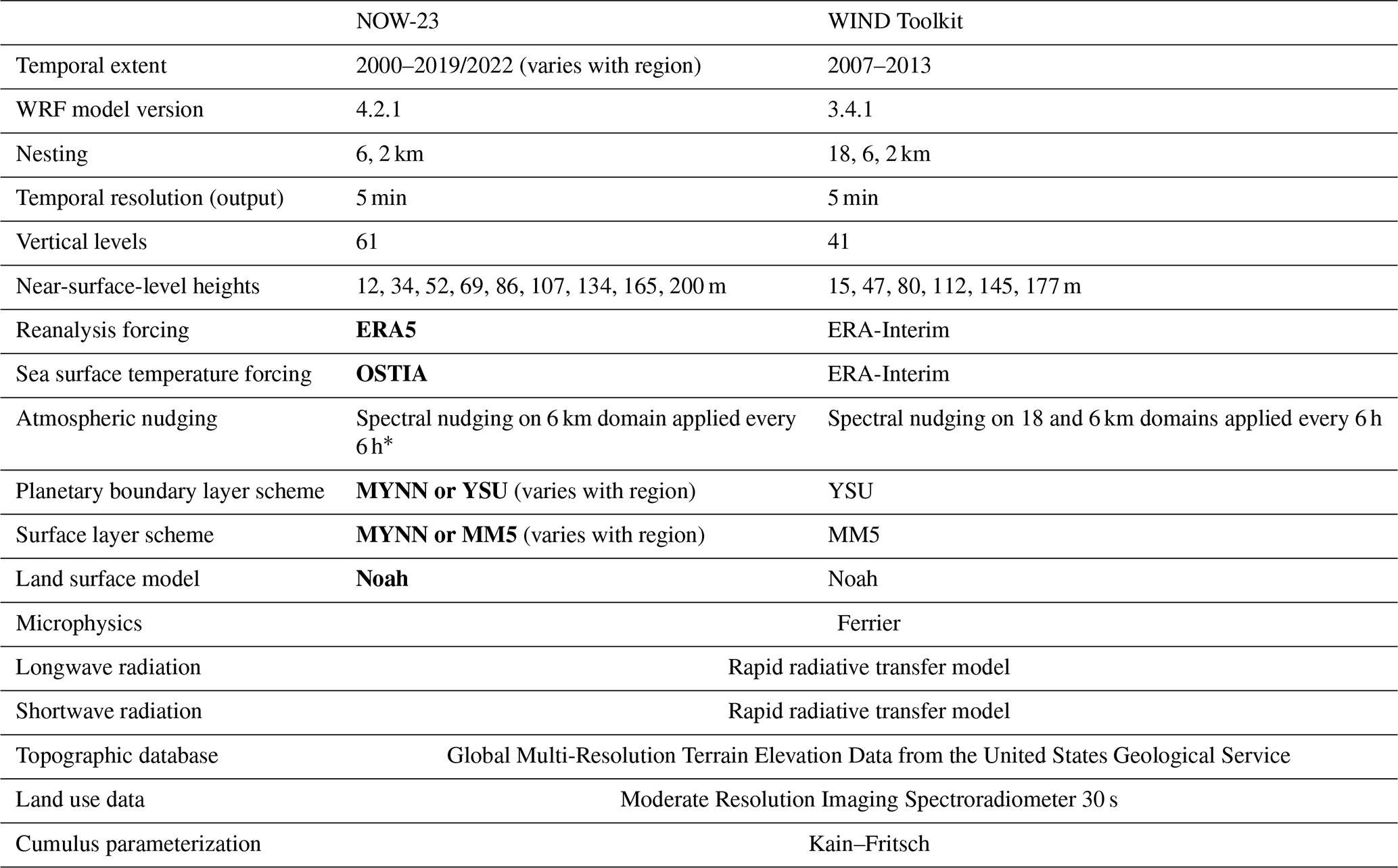
^* Nudging was not applied to the Mid-Atlantic, Great Lakes, North Pacific, and Hawaii regions. Tests showed that nudging does not have a significant impact for offshore regions when using regional domains and monthly runs.

Table 1 shows that some of the WRF model parameters were regionally tuned in NOW-23. In fact, many different setup choices need to be made before running a WRF model simulation so that multiple simulations run with different setups will lead to a range of modeled conditions. It is therefore essential to tune the WRF model setup to obtain accurate model predictions over the region of interest. For the majority of the regions modeled in this work, we considered and run multiple WRF model setups (i.e., a WRF model ensemble) over a 1-year period and validated them against available observations to select the configuration that is best suited for long-term offshore wind resource assessment in each region. To determine which set of WRF model setups to consider in our validation experiments, we leveraged recent research in the area to understand which choices strongly impact the WRF-modeled wind resource. A detailed list of the studies on the WRF-predicted wind speed sensitivity to the WRF model setup is included in Optis et al. (2020c). Here, we highlight the exhaustive effort by Hahmann et al. (2020) to develop the New European Wind Atlas (NEWA), as well as an offshore analysis of the WRF model sensitivity that NREL recently completed in partnership with Rutgers University Center for Ocean Observing Leadership (Optis et al., 2020b). Based on the findings from recent scientific literature on the topic, we identify the following five model setup choices as the most influential on the WRF-predicted wind resource: the reanalysis forcing product, the planetary boundary layer (PBL) scheme, the sea surface temperature (SST) product, the land surface model (LSM), and the surface layer scheme. For each region where we run a short-term WRF model ensemble, we consider a subset of setups resulting from the combination of the following choices:

• Reanalysis forcing product. Reanalysis products are used as boundary conditions for the WRF model. We consider the state-of-the-art ERA5 reanalysis product developed by the European Centre for Medium-Range Weather Forecasts (Hersbach et al., 2020) and the Modern-Era Retrospective analysis for Research and Applications, Version 2 (MERRA-2; Gelaro et al., 2017) developed by the National Aeronautics and Space Administration (NASA). Both of these reanalysis products have been widely used in wind-energy-related applications and represent some of the most advanced reanalysis products available to date. Data from ERA5 are provided at an hourly resolution and 0.25° × 0.25° horizontal resolution. MERRA-2 also provides data at an hourly resolution but at a coarser horizontal resolution of 0.50° × 0.625°.

• Planetary boundary layer scheme. The choice of the PBL scheme has critical consequences in terms of how the WRF model will model turbulent exchanges in the atmospheric boundary layer, and it is expected to have a significant impact on the wind speed predictions. Here, we consider the Mellor–Yamada–Nakanishi–Niino (MYNN; Nakanishi and Niino, 2009) and Yonsei University (YSU; Hong et al., 2006) PBL schemes. These parameterizations are widely considered the two most popular PBL schemes in the WRF model, especially when considering wind-related applications; YSU was used in the WIND Toolkit and MYNN in the NEWA (Dörenkämper et al., 2020).

• Sea surface temperature product. Because the focus of this research effort is on offshore wind, the choice of the sea surface temperature product, which acts as a lower boundary condition for the WRF model, should also be assessed in detail. We note that the same considerations apply to the Great Lakes too. The first SST product we consider is the Operational Sea Surface Temperature and Ice Analysis (OSTIA) data set produced by the UK Met Office (Donlon et al., 2012; Hirahara et al., 2016), which provides data at $\mathrm{1}/\mathrm{20}$° horizontal resolution and is the standard product included in both ERA5 and MERRA-2. Next, we consider the National Centers for Environmental Prediction (NCEP) real-time global SST product (Thiébaux et al., 2003) at $\mathrm{1}/\mathrm{12}$° horizontal resolution.

• Land surface model. The choice of the land surface model can have a significant impact on offshore waters near the coast, as the LSM regulates the exchange of energy and water fluxes between the land surface and the atmosphere. We consider the Noah LSM and the updated Noah multiparameterization (Noah-MP) LSM (Niu et al., 2011).

• Surface layer scheme. Finally, the surface layer scheme handles how fluxes of heat, momentum, and moisture move from the surface to the boundary layer above. We consider the MM5 (Grell et al., 1994; Jiménez et al., 2012) and MYNN (Olson et al., 2021) surface layer schemes. Both are built on the Monin–Obukhov similarity theory, but the MYNN parameterization has been designed to specifically interface with the MYNN PBL scheme.

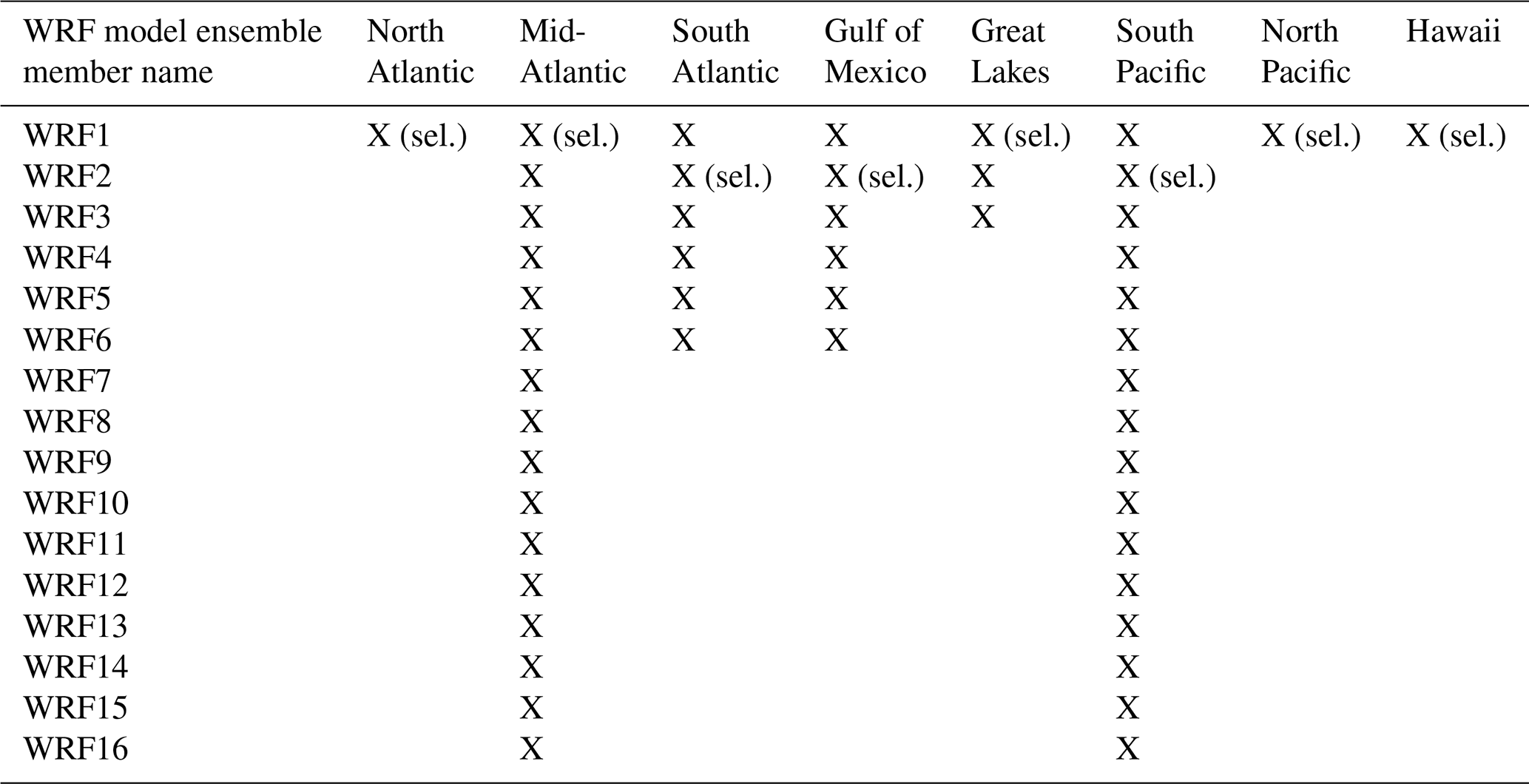
We consider up to 16 WRF model ensemble members resulting from a combination of the choices above, as detailed in Table 2. Table 3 summarizes the ensemble members that are considered for model setup selection and validation in each NOW-23 region, and the selected setup that is used for the long-term model run, as detailed in the next sections.

Table 2 List of the 16 WRF model ensemble members considered for NOW-23 setup selection and validation.

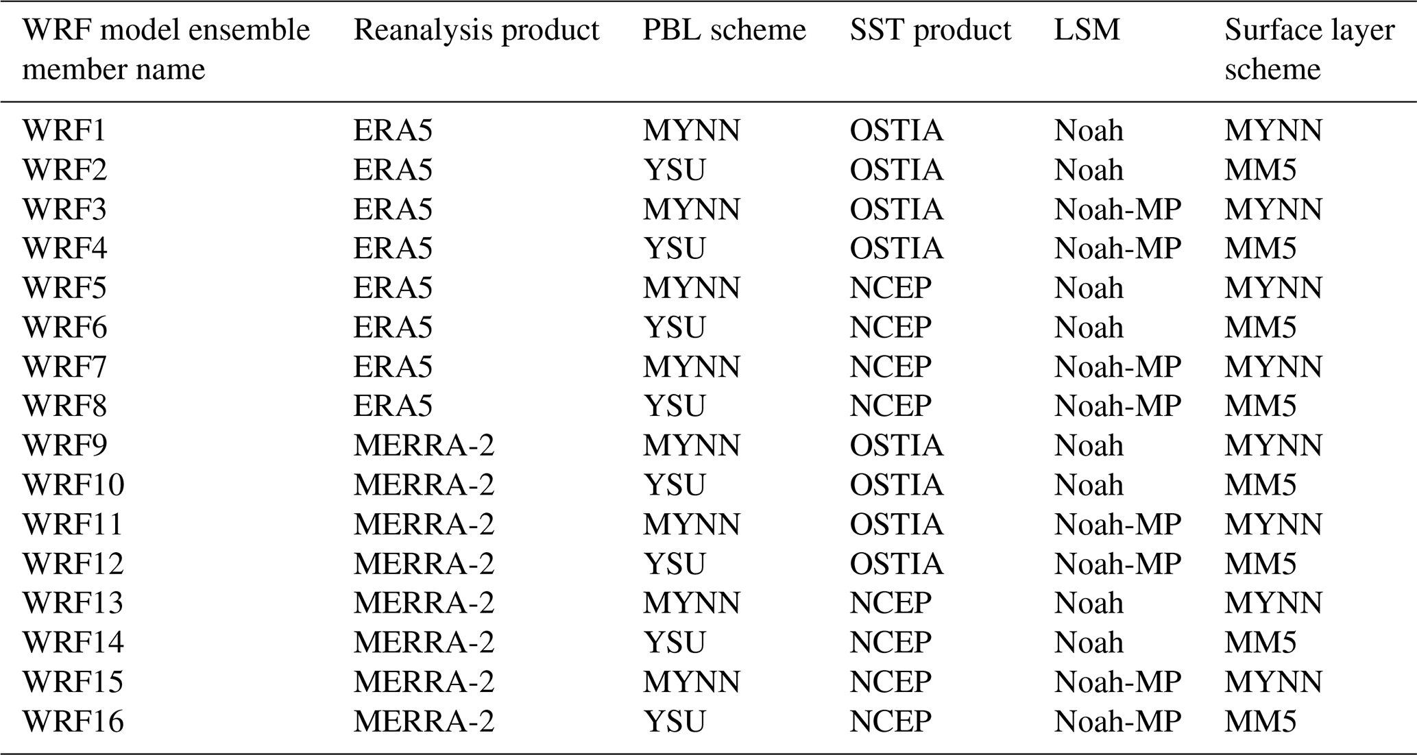
Table 3 WRF model ensemble members used for setup selection and validation in each NOW-23 region. The setup selected (sel.) and used for the long-term NOW-23 data set in each region is also highlighted.

In the majority of the offshore regions modeled in NOW-23, we leverage available offshore or coastal observations to determine the best-performing WRF model setup. All the observational data sets used in the development of NOW-23 are shown in the map in Fig. 2 and will be described in detail in the next sections for each offshore region. In general, we use data from all of the offshore lidars for which we have access. We also consider observations collected by near-surface buoys from the National Data Buoy Center (NDBC) and coastal radars, as resources allow.

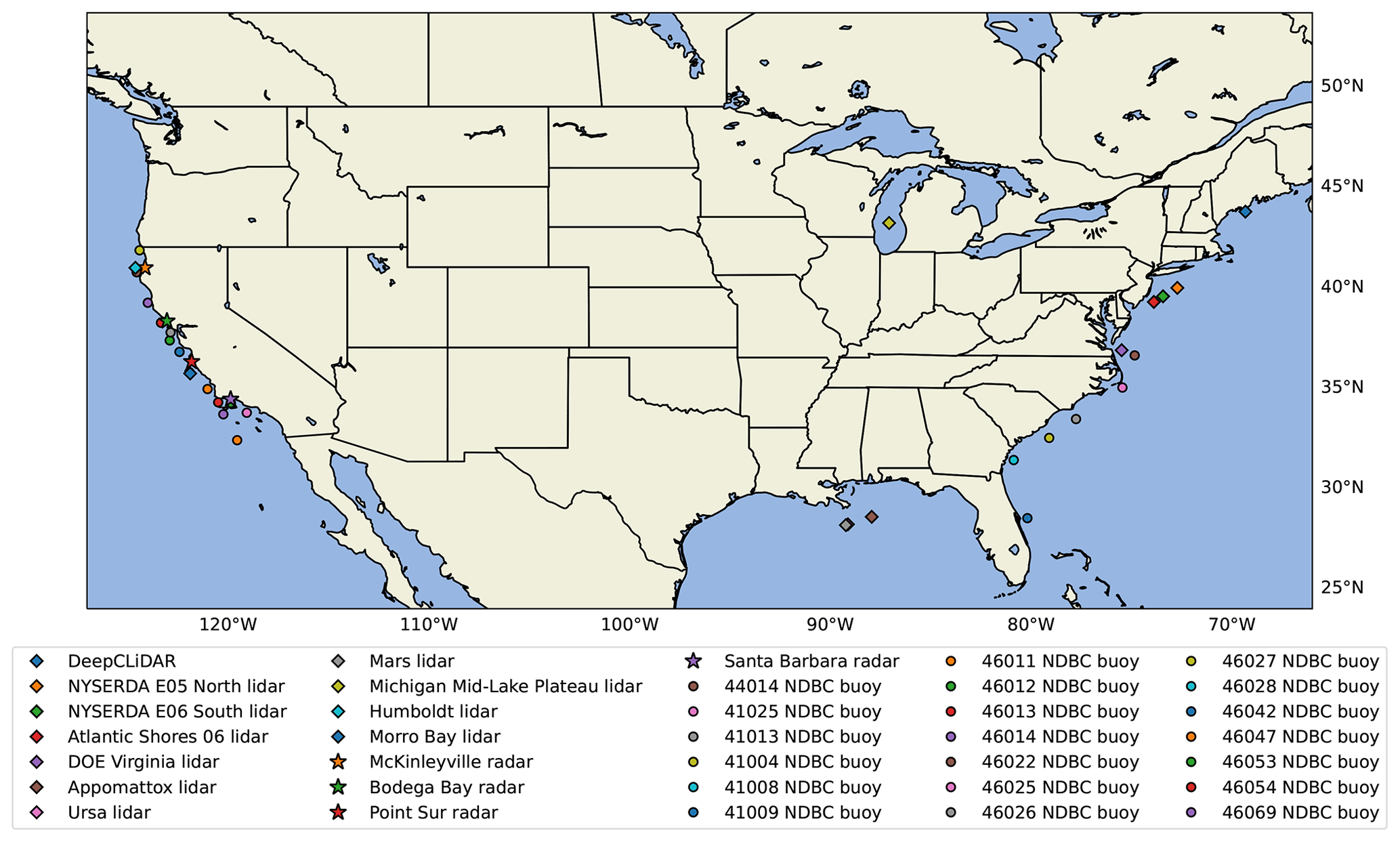
Figure 2 Map of the observational data sets used to validate the NOW-23 data set.

We base our validation approach on the best practices detailed in Optis et al. (2020a) and, whenever possible, use multiple error metrics between modeled and observed wind speed for our model validation and setup selection:

• bias,

• centered (or unbiased) root mean square error (cRMSE),

• Pearson's correlation coefficient (r), and

• a comparison between the standard deviation of modeled and observed wind speed.

A perfect model setup would have zero bias, zero cRMSE, r=1, and a modeled wind speed standard deviation equal to that of the observed wind. To summarize the latter three metrics, we adopt the Taylor diagram (Taylor, 2001), which is a mathematical diagram that graphically summarizes model skills in terms of cRMSE, r, and standard deviation on a single plot.

3 NOW-23 data set in the Mid-Atlantic region

We start the description of the NOW-23 data set with the Mid-Atlantic domain, an area with multiple publicly available observational data sets of hub height offshore wind and therefore an ideal region to detail the validation approach adopted to develop NOW-23.

For the Mid-Atlantic region, we consider all the combinations resulting from the choices of reanalysis product, SST product, PBL scheme, and LSM detailed in Sect. 2. We do not consider for this region the impact of the surface layer scheme due to computational limitations; we use the MYNN surface layer option when the MYNN PBL scheme is used and the MM5 option with the YSU PBL scheme. These combinations result in 16 different WRF model setups (Table 3) which are all run over 1 year (using the general approach described in Sect. 2) from 1 September 2019 to 31 August 2020.

To select the best-performing WRF model setup in the region, which will be used for the long-term NOW-23 data set, we compare modeled wind speed from the 16 WRF model setups against observations collected by the three ZephIR ZX300M floating lidars, as shown in the map in Fig. 2. Two of the three lidars were deployed by the New York State Energy Research and Development Authority (NYSERDA). The lidar on buoy E05 north is located at 39.97° N, 72.72° W; the buoy E06 south lidar is located at 39.55° N, 73.43° W. Wind speed and wind direction data for both lidars are available every 20 m from 20 to 200 m a.s.l. (above sea level) and are publicly distributed at 10 min resolution after proprietary quality checks have been applied to the data. For both lidars, we use observations collected between 4 September 2019 and 31 August 2020. The third lidar was deployed by Atlantic Shores Offshore Wind, LLC, closer to the coastline at 39.27° N, 73.88° W. This lidar measures wind speed every 20 m from 40 to 200 m above the surface. For this instrument, we leverage observations from 26 February 2020 (the start of its deployment) to 31 August 2020.

First, we assess the variability in the mean wind profiles across the 16 1-year WRF model ensembles (Fig. 3). We color code the mean wind profiles in terms of the PBL scheme used by the various ensemble members because, as will be detailed later, in some offshore regions we see a significant deviation in modeled wind speeds between the MYNN and YSU PBL schemes. In the Mid-Atlantic, the WRF model ensemble members that adopt the YSU PBL scheme model generally weaker wind speeds compared to MYNN at all three lidar locations, with the largest deviations occurring below 100 m a.s.l., with differences generally lower than 0.5 m s⁻¹ on average. While the MYNN generally slightly overestimates wind speeds below 50 m a.s.l., we find that all the considered setups underestimate wind shear, thus resulting in a slightly negative bias higher aloft.

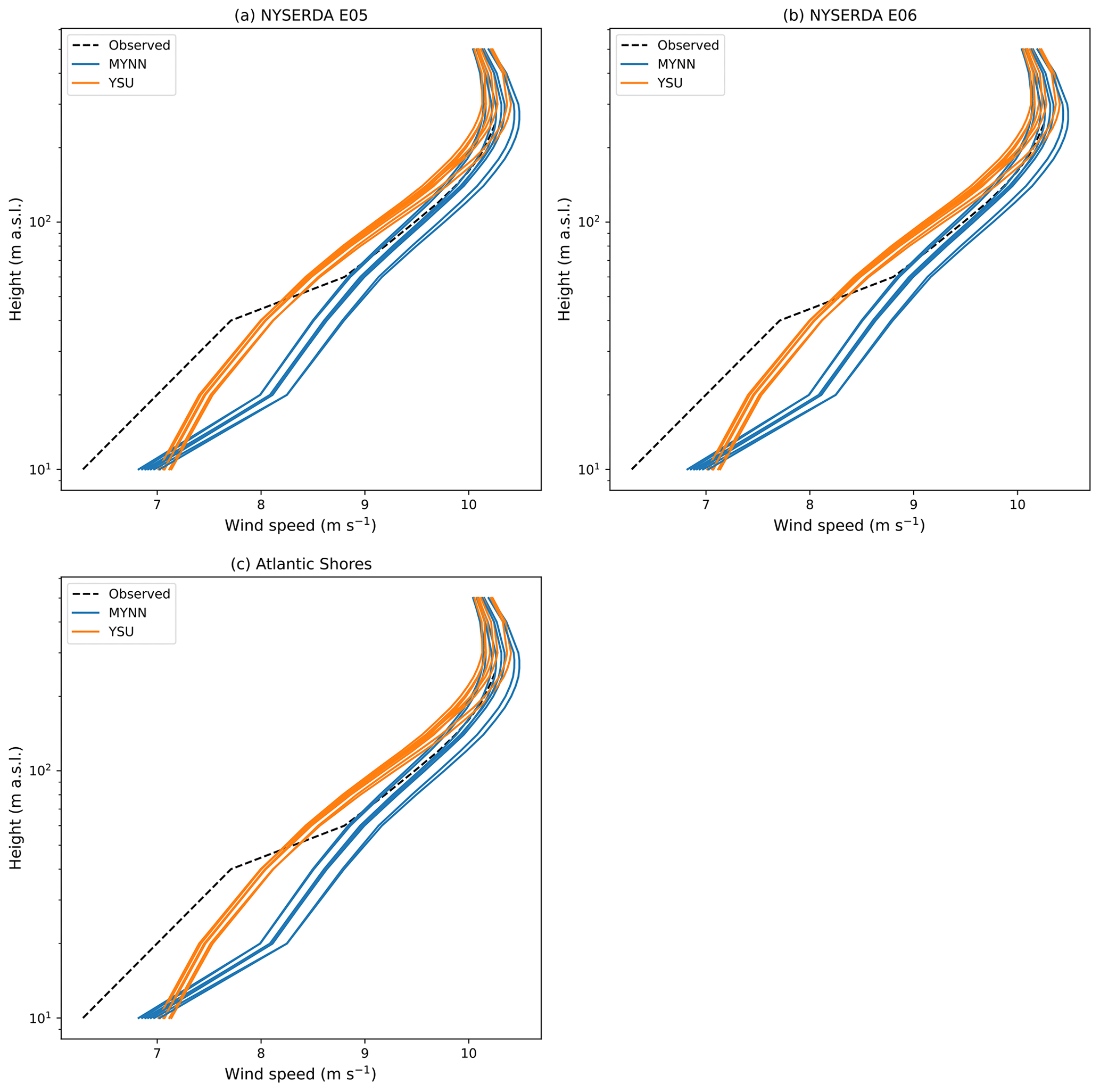
Figure 3 Mean wind speed profiles from the 16 WRF model ensemble members and observed values at the location of the (a) NYSERDA E05 north lidar (from 4 September 2019 to 31 August 2020), (b) NYSERDA E06 south lidar (from 4 September 2019 to 31 August 2020), and (c) Atlantic Shores lidar (from 26 February 2020 to 31 August 2020).

We now dive deeper into the validation by assessing more quantitative performance metrics. All three lidars in this region provide good measurements at a wide range of heights of interest for wind energy development. To capture the WRF model performance across all heights, we perform our model validation in terms of the rotor-equivalent wind speed (REWS), which is the wind speed corresponding to the kinetic energy flux through a turbine's swept-rotor area, when accounting for the vertical shear. The REWS is calculated as

$$\begin{array}{}\text{(1)}& \text{REWS}={\left(\sum _{i=\mathrm{1}}^n{\text{WS}}_i^{\mathrm{3}}{\displaystyle \frac{A_i}{A}}\right)}^{\mathrm{1}/\mathrm{3}},\end{array}$$

where WS_i is the wind speed at the height level i, n is the number of available heights across the wind turbine rotor disk, A is the whole area of the turbine rotor disk, and A_i is the area of the ith segment; i.e., the area for which WS_i is representative. Here, we consider the 10 MW turbine from Beiter et al. (2020) representative of a typical commercial offshore turbine, with a rotor diameter of 196 m and a hub height of 128 m. We consider horizontal layers in the turbine rotor disk to be equally spaced every 20 m from 30 to 190 m a.s.l., each associated with observed and modeled wind speed every 20 m from 40 to 180 m a.s.l. Finally, the top layer extends from 190 to 226 m and is associated with the 200 m wind speed, given the lack of lidar observations higher than 200 m a.s.l. While bigger turbines reaching higher heights are being installed in the region, the highest height of lidar observations at 200 m limits our ability to consider larger machines here.

We calculate bias, cRMSE, correlation, and standard deviation in terms of observed and modeled 10 min REWS from all 16 WRF model ensemble members and summarize results in the Taylor diagrams in Fig. 4. Ideally, a perfect member would be represented in the Taylor diagram by a point on top of the black star in each diagram, which represents the observed values. At all three lidars, we find that the WRF model ensemble members that use MERRA-2 as reanalysis forcing (WRF9 through WRF16 in red shades in the diagrams) show a significantly worse performance compared to the setups forced with ERA5, with larger cRMSE and lower correlation. Also, the setups that adopt the YSU PBL scheme (even numbers) have a slightly better match with the standard deviation of the observed wind resource but also a larger negative bias at all three offshore lidars compared to the MYNN setups (odd numbers), as already noticed from the mean wind profile comparison above. The use of the Noah LSM provides slightly better results than the Noah-MP LSM in terms of correlation and cRMSE. Finally, we see that the choice of the SST product does not have a significant impact on the validation metrics.

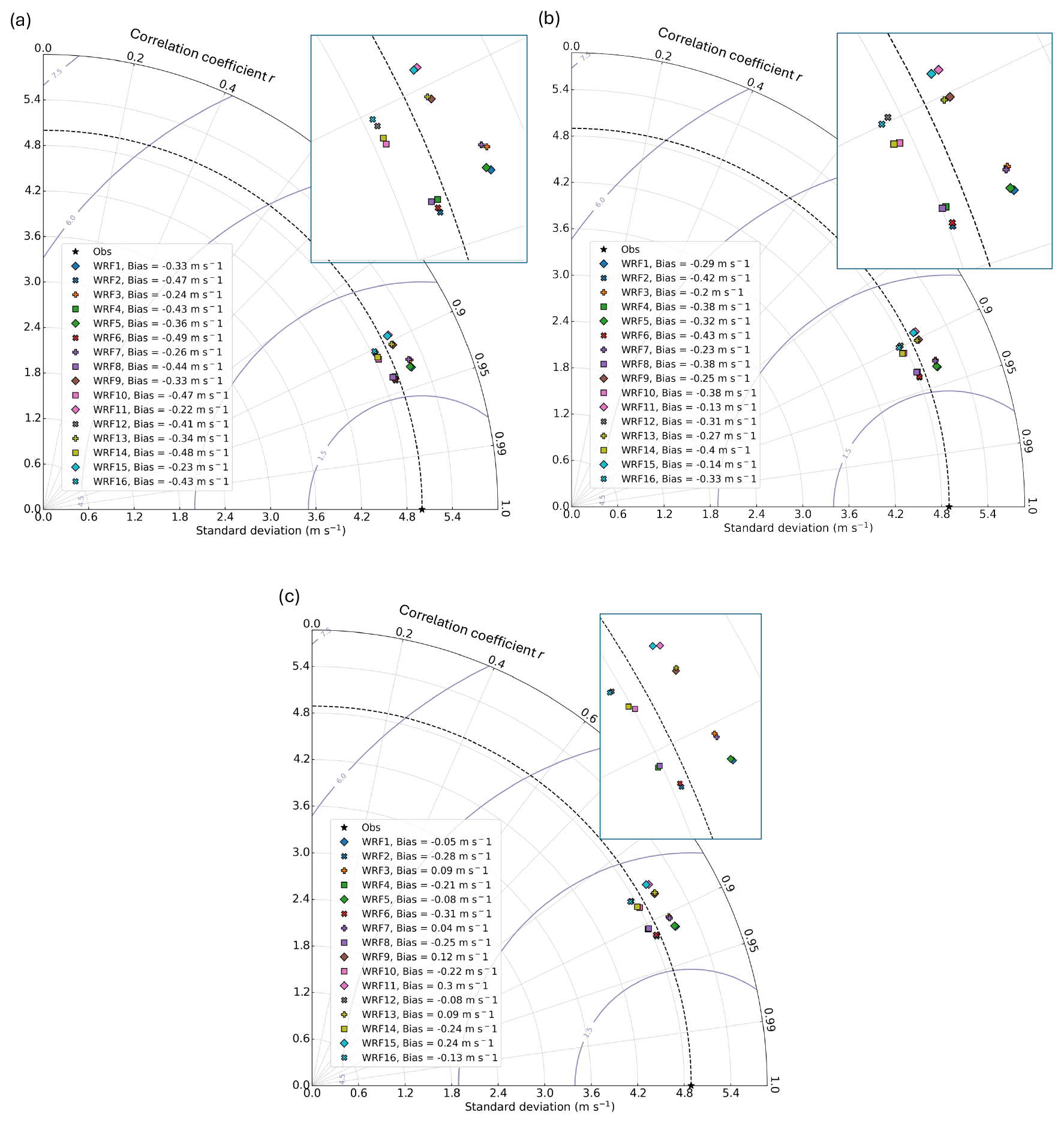
Figure 4 Taylor diagram of the 10 min REWS from the 16 WRF model ensemble setups at the location of the (a) NYSERDA E05 north lidar (from 4 September 2019 to 31 August 2020), (b) NYSERDA E06 south lidar (from 4 September 2019 to 31 August 2020), and (c) Atlantic Shores lidar (from 26 February 2020 to 31 August 2020). For each diagram, a zoomed-in inset is also included.

Finally, we evaluate whether our choice of using a 1-month WRF model re-initialization period has an impact on the model performance. To do so, we take the wind speed modeled by the 1-year WRF1 setup and check whether its performance against the observations from the two NYSERDA lidars gets worse in the latter part of each calendar month, again in terms of REWS. For all metrics, we report no sign of performance degradation with time (figure not shown), which confirms the solidity of the modeling approach used.

The validation results across all three lidars show that WRF1 and WRF3 are the best-performing setups in the region. While there is no clear winner between the two in terms of bias, WRF1 (i.e., the setup using the Noah LSM) provides lower cRMSE and higher correlation compared to WRF3 (i.e., the setup using the Noah-MP LSM), so we employ WRF1 for the long-term NOW-23 simulation (Table 3), which covers the period from 1 January 2000 to 31 December 2020. We note that additional details on the validation of the WRF1 model setup are provided in Pronk et al. (2022), where we assess the diurnal and annual variability in the WRF1 model setup performance, and compare it to the skills of the ERA5 reanalysis product used to force WRF.

The 21-year mean wind speed at 160 m a.s.l. for the Mid-Atlantic region is shown in Fig. 5. In Appendix A, we show the diurnal and seasonal variabilities in the long-term wind resource. The mean wind speed is stronger on the northeast portion of the domain, but the long-term averages are particularly good for offshore wind energy purposes in the whole extension of the domain.

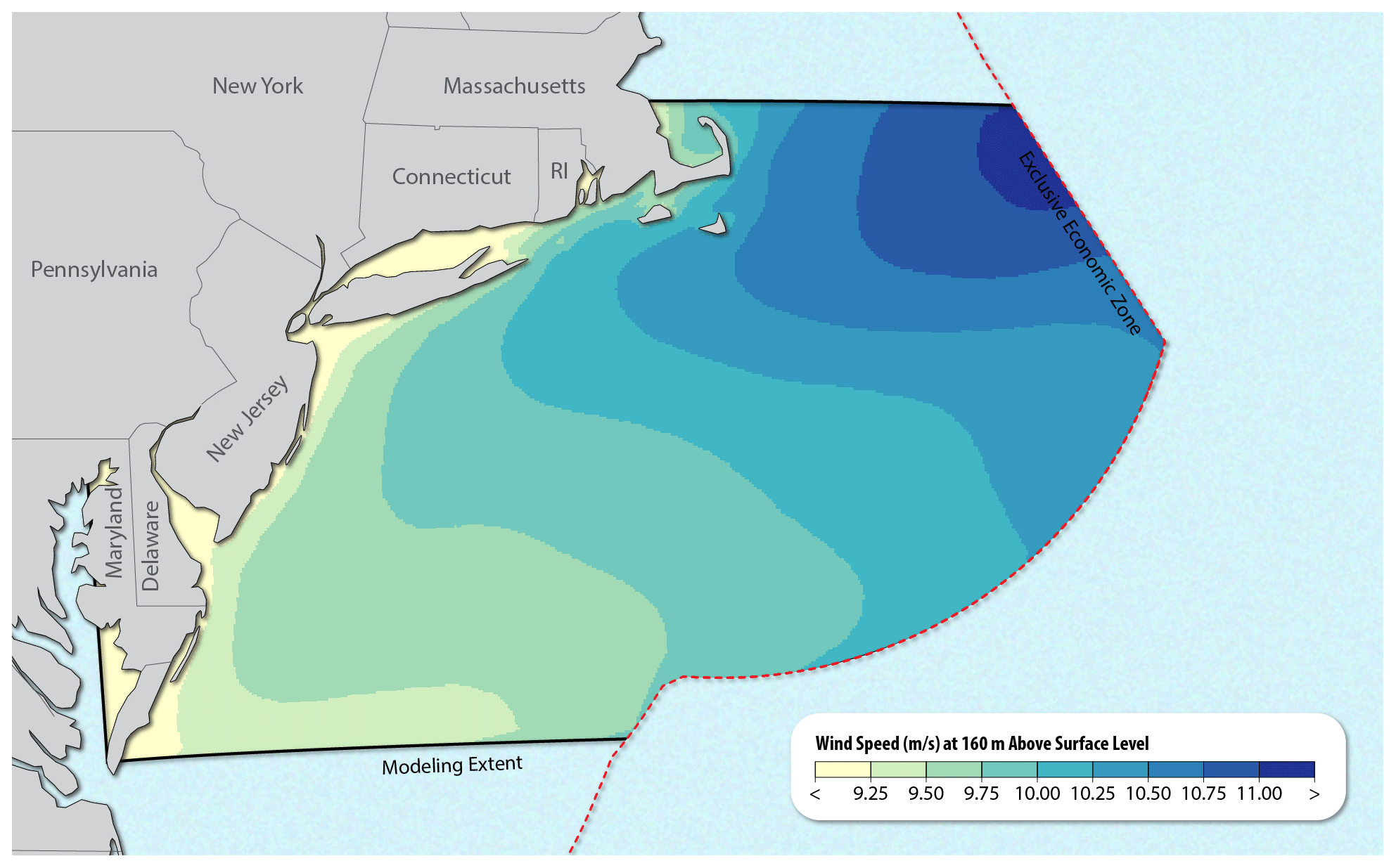
Figure 5 Map of the 21-year (2000–2020) mean wind speed at 160 m a.s.l. for the Mid-Atlantic region. The dashed red line represents the limit of the US EEZ. The continuous black line, where not overlaid with the EEZ boundary, shows the limit of the NOW-23 WRF model domain.

4 NOW-23 data set in the North Atlantic region

We leverage the validation results from the Mid-Atlantic region to infer conclusions about the WRF model setup to use for the long-term wind resource modeling in the adjacent North Atlantic region, where we only have access to very limited hub height observations of wind speed. Given this scenario, and considering the limited computational resources available, in this region we consider a single WRF model setup, using the same choices selected for the creation of the NOW-23 data set in the Mid-Atlantic region.

No hub height observational data sets are publicly available for this region. So, our model validation is constrained to values of mean 40 and 100 m wind speeds taken from 19 February 2016 through 28 October 2016 at the DeepCLiDAR off the Maine coast (43.77° N, 69.33° W; Fig. 2), 1.26 km west of Monhegan island (Viselli et al., 2019, 2022). This floating lidar is a WindCube v2 offshore unit owned and operated by the University of Maine and samples wind speeds between 40 and 200 m at 1 Hz resolution. The NOW-23 research team was not able to secure access to the raw lidar observations, so our validation is limited to the mean wind speed values, as published in Viselli et al. (2022).

Due to the particularly small sample size of available observations, we only compare the observed and modeled mean 40 and 100 m wind speed at the DeepCLiDAR location over the deployment period of the lidar. We find good agreement between modeled and observed data at 100 m a.s.l., whereas the model slightly overestimates wind speed at 40 m a.s.l. (Fig. 6).

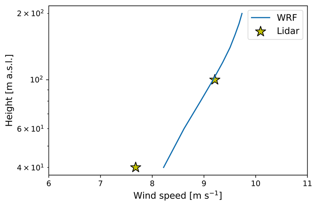
Figure 6 Mean wind speed profiles from the WRF model run (WRF1 setup) and observed mean wind speed at 40 and 100 m a.s.l. at the location of the DeepCLiDAR buoy from 19 February 2016 through 28 October 2016.

The limited validation confirms that the chosen WRF model setup has good agreement with the mean observations from the lidar at the considered location, so we use the WRF1 setup to create the NOW-23 simulation in this region (Table 3), which covers the period from 1 January 2000 to 31 December 2020.

The 21-year mean wind speed at 160 m a.s.l. for the North Atlantic region is shown in Fig. 7. Its seasonal and diurnal variabilities are shown in Appendix A. In this region, we find that the dominant gradient in mean wind speed is aligned with the east–west direction, with stronger wind speeds observed further offshore. As observed in the Mid-Atlantic region, the large mean wind speed values make this region well suited for offshore wind energy.

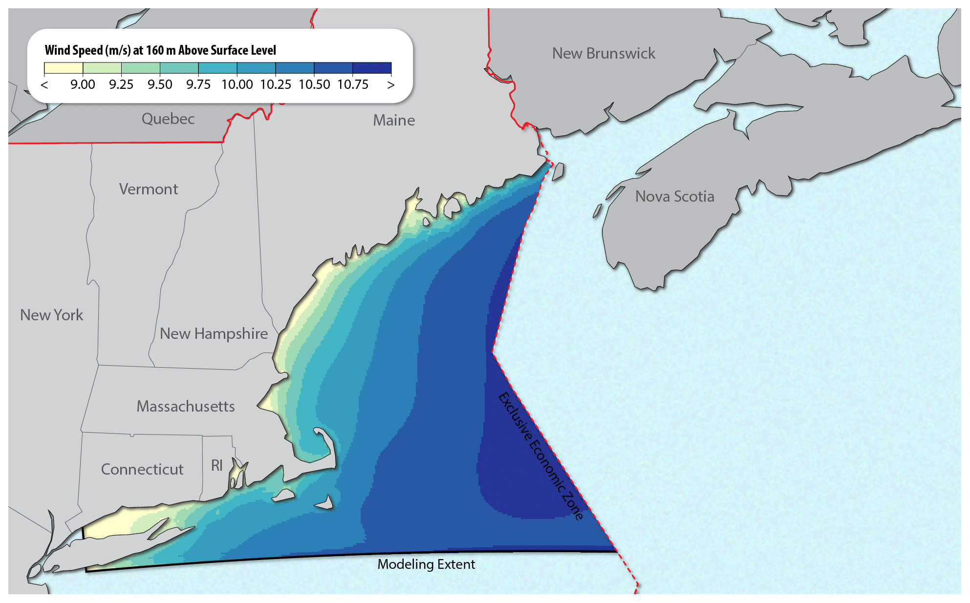
Figure 7 Map of the 21-year (2000–2020) mean wind speed at 160 m a.s.l. for the North Atlantic region. The dashed red line represents the limit of the US EEZ. The continuous black line, where not overlaid with the EEZ boundary, shows the limit of the NOW-23 WRF model domain.

5 NOW-23 data set in the South Atlantic region

For the South Atlantic region, we consider six WRF model setup combinations resulting from the choices of PBL scheme, surface layer scheme, and LSM, as detailed in Sect. 2. We do not consider for this region the impact of the SST (we only consider the OSTIA product, which has shown larger accuracy than the NCEP product based on the sensitivity analysis in the Mid-Atlantic region) and of the reanalysis product (because we found that ERA5 has significantly better performance than MERRA-2 in the Mid-Atlantic region). We run all six setups (Table 3) across two sets of simulations (using the general approach described in Sect. 2), with one covering the whole year of 2015 and one covering the period from 1 June 2020 to 31 December 2020.

The main validation data set we use in this region is represented by observations collected by the U.S. Department of Energy (DOE) lidar located off the Virginia coast (36.87° N, 75.49° W) (Shaw et al., 2020). This lidar recorded observations from 11 December 2014 to 31 May 2016. For our validation, we use data from the whole year of 2015 to ensure all seasons are equally represented. Conversations with the instrument mentors at Pacific Northwest National Laboratory (PNNL) revealed that only the lidar measurements at 90 m are unaffected by biases, so we limit the NOW-23 model validation to that height. Whereas algorithms to bias-correct the lidar measurements at other heights have been developed, we prefer not to use them here to avoid introducing additional uncertainty in the validation. Additionally, the Avangrid company performed a validation using proprietary data from their Kitty Hawk north lidar, covering the period from 1 June to 31 December 2020. Finally, we note how both the Virginia and Kitty Hawk north lidars are near the northern edge of our regional domain. Therefore, to improve the spatial coverage of the NOW-23 validation in the region, we leverage observations from six NDBC buoys across the domain to validate modeled near-surface atmospheric stability, quantified in terms of the difference between air temperature and sea surface temperature, over 2015.

Figure 8 shows the mean modeled wind profiles over 2015 at the location of the Virginia lidar for the six WRF model setups, as well as the mean 90 m wind speed from the DOE Virginia lidar over the same year. In general, a limited spread between the different WRF model setups appears, and all setups provide a limited overestimation of mean wind speed at 90 m a.s.l. compared to the lidar observations.

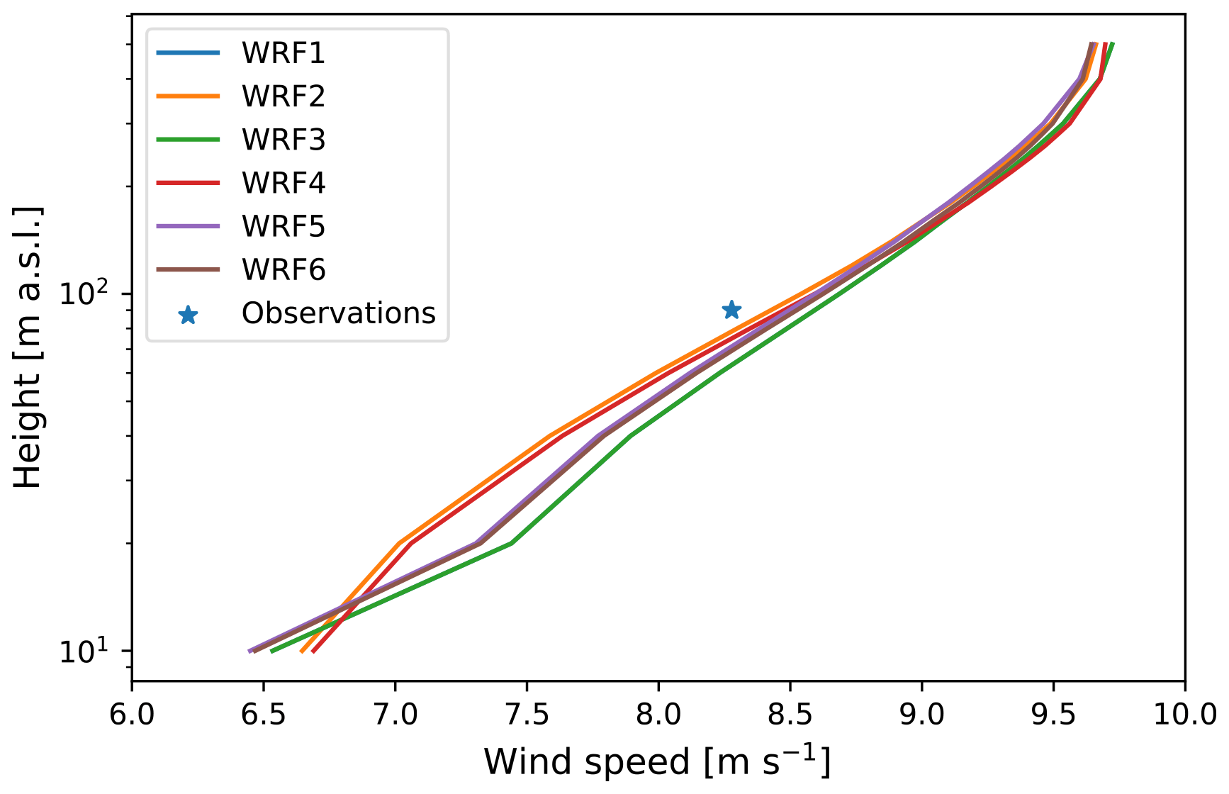
Figure 8 Mean modeled wind speed profiles from 1 January 2015 to 31 December 2015 from the six WRF model setups considered for the sensitivity analysis and mean observed winds at 90 m from the DOE Virginia lidar.

We formalize the regional validation with the Taylor diagram in Fig. 9, again at 90 m a.s.l., using wind speed at 10 min resolution. The diagram reveals that the WRF2 setup performs best in the South Atlantic domain, with a low bias of +0.11 m s⁻¹, the highest Pearson’s correlation coefficient (r=0.83), the lowest cRMSE (2.44 m s⁻¹), and the best match with observed wind speed standard deviation across all the WRF model ensemble members.

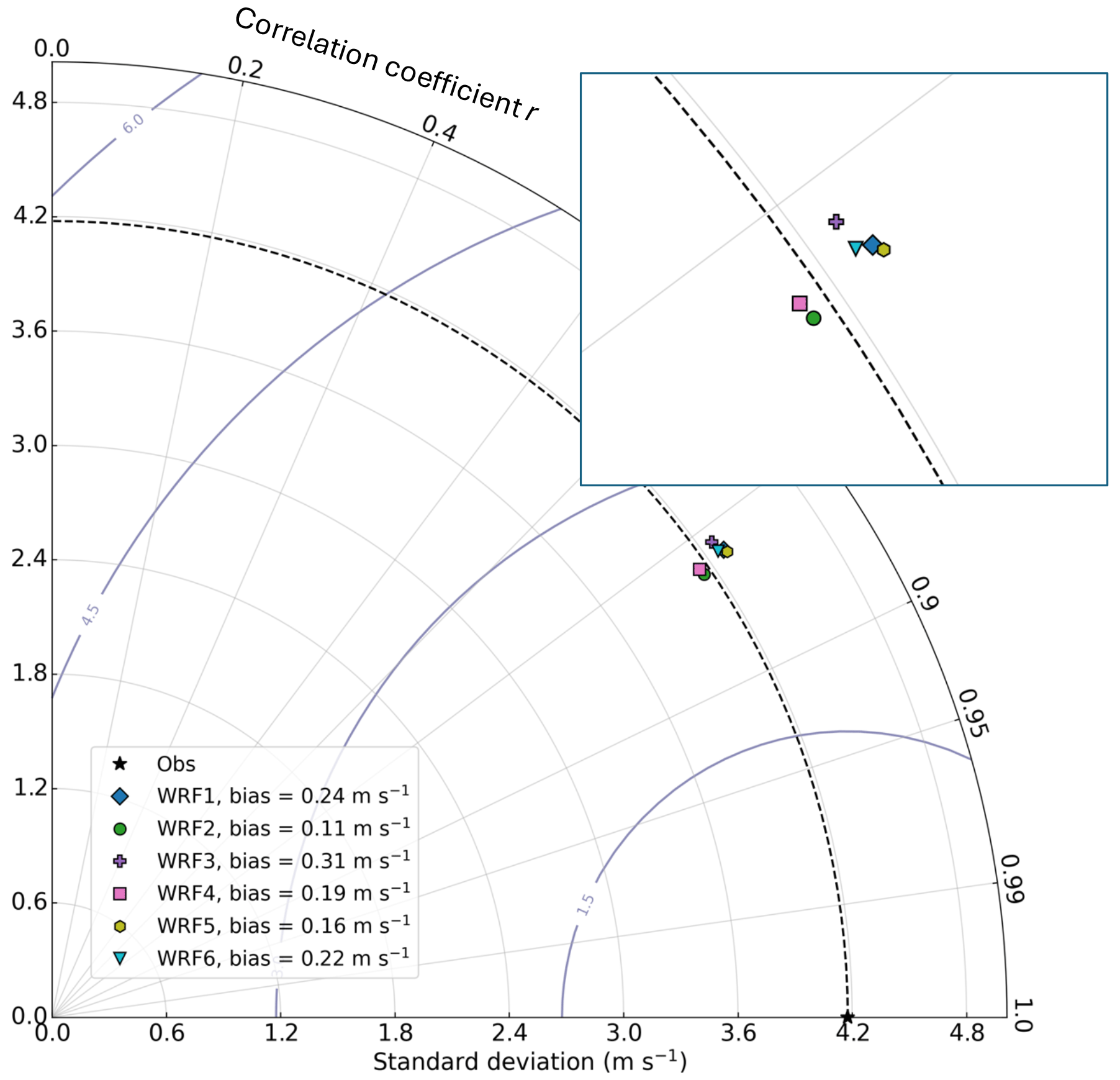
Figure 9 Taylor diagram of the 90 m wind speed from the six WRF model ensemble setups at the location of the DOE Virginia lidar using 10 min data. Data from 1 January 2015 to 31 December 2015. A zoomed-in inset is also included.

Avangrid's Kitty Hawk north lidar data are proprietary, and therefore only the following qualitative results were shared with the NOW-23 team after the company compared the six WRF model setups against their lidar observations over the last 7 months of 2020:

• All WRF model ensemble members performed well in terms of their wind rose.

• Overall, ensemble members WRF2 and WRF4 performed the best for both wind speed and wind shear profiles.

• Some specific months were challenging to model for all considered ensemble members.

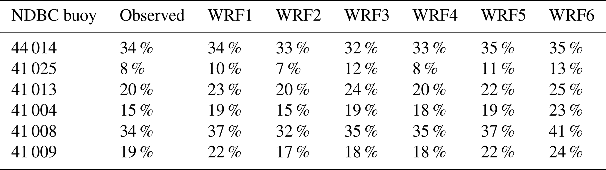
Next, we leverage the more extensive spatial coverage of the NDBC buoys in the region to validate modeled atmospheric stability near the surface, and we summarize these results in Table 4. We consider a positive difference between air temperature (at ∼ 4 m a.s.l. for the NDBC buoys; 2 m a.s.l. for the WRF model simulations) and sea surface temperature as a proxy for stable conditions and report its observed and modeled temporal frequency over 2015 in the table. The WRF model setups that use MYNN as a PBL scheme (WRF1, WRF3, WRF5, and WRF6) overestimate atmospheric stability. On the other hand, YSU-modeled stability (WRF2 and WRF4) is generally more aligned with observations across the whole region. This result, if confirmed at hub heights, is consistent with the larger wind speed bias that the MYNN setups have in the Taylor diagram. In fact, under stable conditions, winds aloft can decouple from surface effects and greatly accelerate.

Table 4 Frequency of near-surface stable conditions from NDBC buoy observations and the six WRF model ensemble members over 2015.

Finally, as done in the Mid-Atlantic domain, we check for an impact of using a 1-month WRF model re-initialization period in our simulations. To do so, we take the WRF2 setup for 2015 and check whether its performance against the DOE Virginia lidar observations gets worse in the latter part of each calendar month. For all metrics, we see no sign of performance degradation with time (figure not shown), as already observed further north along the Mid-Atlantic coast.

Our validation analysis across all considered instruments and atmospheric variables reveals that the WRF2 setup is the best-performing one in this region, and therefore we use this setup for the NOW-23 long-term simulation, which covers the period from 1 January 2000 to 31 December 2020. We note that this setup differs from the setup used in the adjacent Mid-Atlantic region so that some discontinuity at the interface between the two domains is expected. Such a difference should, however, be limited in magnitude given the minimal difference between the mean wind profiles near the northern edge of the domain in Fig. 8. This discrepancy is described in further detail in Appendix B.

The 21-year mean wind speed at 160 m a.s.l. for the South Atlantic region is shown in Fig. 10. Wind speed is, on average, stronger in the northern half of the domain, with a clear north–south gradient that leads to mean differences of more than 2 m s⁻¹ between the northern and southern edges of the modeled region. We note that we had to limit the extent of the WRF model domain for this large region to reduce computational requirements so that the northern portion of the domain does not reach the limit of the US EEZ. Appendix A shows the diurnal and seasonal variability in the 160 m wind resource.

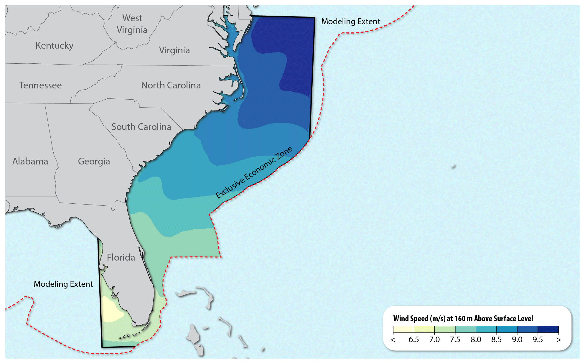
Figure 10 Map of the 21-year (2000–2020) mean wind speed at 160 m a.s.l. for the South Atlantic region. The dashed red line represents the limit of the US EEZ. The continuous black line, where not overlaid with the EEZ boundary, shows the limit of the NOW-23 WRF model domain.

6 NOW-23 data set in the Gulf of Mexico

For the Gulf of Mexico, we consider six ensemble members (Table 3). We only consider ERA5 as reanalysis forcing and OSTIA as SST product for the same considerations listed for the South Atlantic domain. We test both the MYNN and YSU PBL schemes, each associated with the MYNN and MM5 surface layer scheme, respectively. We also consider the impact of the Noah and Noah-MP LSMs. We run the six ensemble members over the year 2020.

Observational wind speed data needed for model setup choice and validation were provided by Shell at three different ZX300 lidars south of the Louisiana coast (Fig. 2). These lidars, named Mars, Ursa, and Appomattox, are located on separate floating oil platforms ∼ 50 m above the ocean and sample winds up through ∼ 150 m above the ocean surface. Data are available from Mars and Ursa for all of 2020, whereas measurements at Appomattox are only available from January through August 2020.

Several buildings and structures are present on the Shell oil platforms. To minimize their wake impacts on the lidar observations, we perform our validation at 140 m a.s.l. (i.e., the maximum common height between the lidars and the WRF model simulations). Figure 11 shows the Taylor diagrams at the three lidars using 10 min data. At all three locations, the WRF2 setup outperforms the other five simulation setups as it has the smallest bias (still with a limited tendency to under-forecast wind speeds), the smallest cRMSE, and the highest correlation (between 0.7 and 0.8 at each lidar).

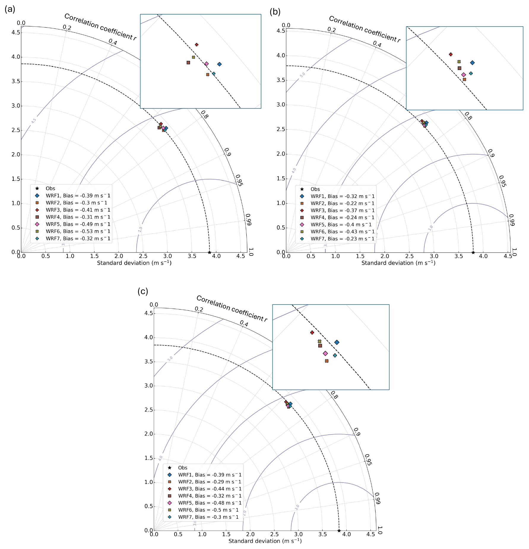
Figure 11 Taylor diagram of the 140 m wind speed from the six WRF model ensemble setups at the location of the (a) Appomattox (from January through August 2020), (b) Ursa (whole year of 2020), and (c) Mars (whole year of 2020) lidars, using 10 min data. For each diagram, a zoomed-in inset is also included.

Our validation analysis shows that the WRF2 setup is the best-performing configuration in this region, and therefore we use this setup for the long-term NOW-23 simulation which covers the period from 1 January 2000 to 31 December 2020.

The 21-year mean wind speed at 160 m a.s.l. for the Gulf of Mexico region is shown in Fig. 12, and Appendix A shows the diurnal and seasonal variability in the modeled wind resource. We observe a clear east–west gradient, with faster winds on the western side of the Gulf and slower winds on the eastern side. This general pattern has also been observed in other studies (de Velasco and Winant, 1996; Zavala-Hidalgo et al., 2014).

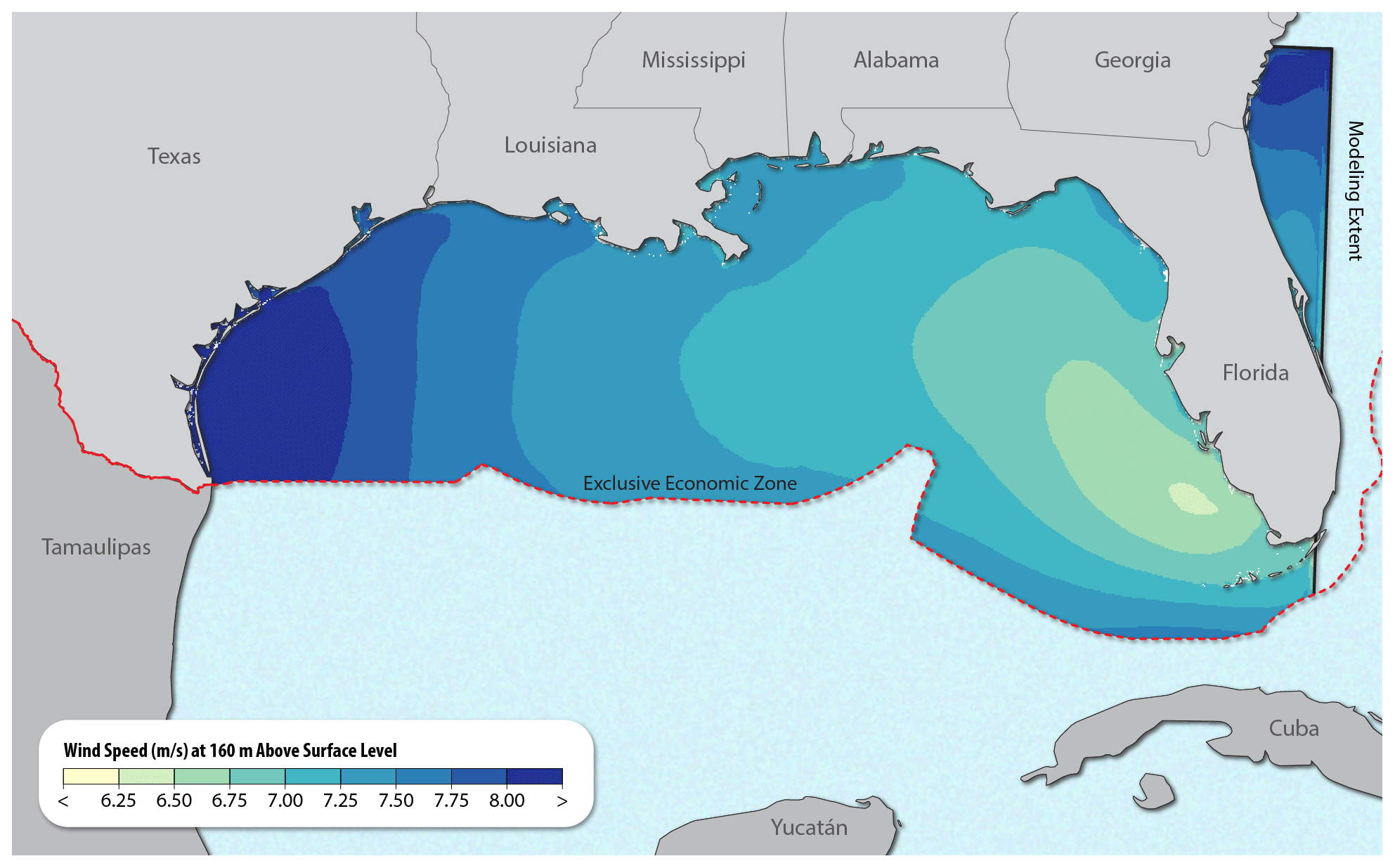
Figure 12 Map of the 21-year (2000–2020) mean wind speed at 160 m a.s.l. for the Gulf of Mexico region. The dashed red line represents the limit of the US EEZ. The continuous black line, where not overlaid with the EEZ boundary, shows the limit of the NOW-23 WRF model domain.

7 NOW-23 data set in the Great Lakes

For the Great Lakes, we only consider three ensemble members (Table 3) by leveraging the results of the model validation in the other offshore regions. Therefore, we only consider ERA5 to be reanalysis forcing and OSTIA to be a SST product. We test both the MYNN and YSU PBL schemes, each associated with the MYNN and MM5 surface layer scheme, respectively. We also consider the impact of the Noah and Noah-MP LSMs. We run the three ensemble members for the year 2012.

To select the best-performing model setup in this region, we leverage observations from one lidar, whose location is shown in the map in Fig. 2. The lidar was deployed in the middle of Lake Michigan and measured wind speed at 75, 90, 105, 125, 150, and 175 m above the surface. For this instrument, we use 10 min average observations from 8 May 2012 to 17 December 2012. We discard data at 175 m as they are deemed unrealistic.

Figure 13 shows the mean wind profiles from the three WRF model ensemble members and the Lake Michigan lidar during the period of record of the lidar observations. All three WRF model setups underestimate wind speed compared to the lidar observations. The setup using the MYNN PBL scheme predicts higher wind speeds compared to the YSU setups in the lowest 200 m, whereas YSU models stronger winds higher aloft. In any case, the difference between all models is rather limited at all heights. We see slight differences between the WRF2 and WRF3 setups, which is an additional indication that using the Noah or Noah-MP LSMs has a limited impact on the mean wind speed profiles, as observed for the other offshore regions.

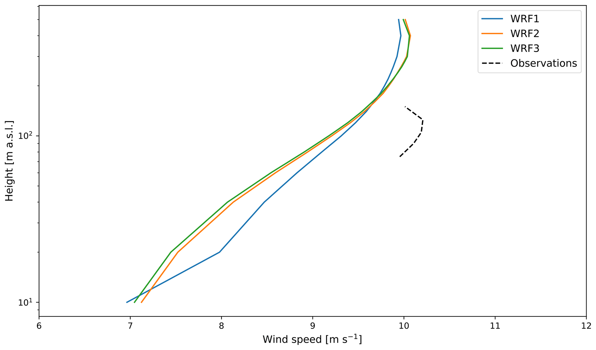
Figure 13 Mean wind speed profiles over the period from 8 May 2012 to 17 December 2012 from the three WRF model ensemble members and lidar observations at the location of the Lake Michigan lidar.

We next consider the Taylor diagram (Fig. 14) at 105 m, using 10 min data. For the modeled data, we linearly interpolate wind speed at 100 and 120 m to allow for a direct comparison with the lidar observations. All three considered WRF model setups show similar performance in terms of bias, correlation, and cRMSE, but the WRF1 setup shows significantly better results in terms of the comparison with the standard deviation of the observed wind speed.

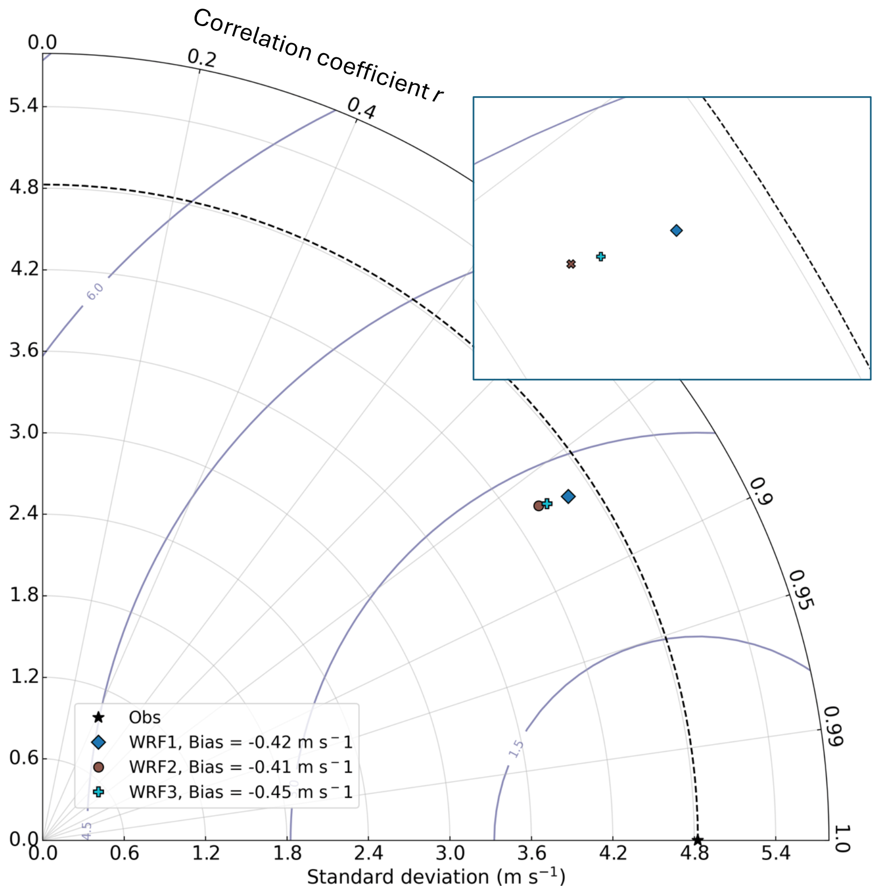
Figure 14 Taylor diagram of the 105 m wind speed from the three WRF model ensemble setups at the location of the Lake Michigan lidar at 10 min resolution. Data from 8 May 2012 to 17 December 2012. A zoomed-in inset is also included.

Our validation analysis shows that the WRF1 setup is the best-performing configuration in this region, and therefore we use this setup for the NOW-23 long-term simulation, which covers the period from 1 January 2000 to 31 December 2020.

The 21-year mean wind speed at 160 m a.s.l. for the Great Lakes region is shown in Fig. 15. Wind speed gets stronger near the center of the lakes, especially for the larger lakes (Michigan, Superior, and Huron). The magnitude of the mean wind speed across the domain is similar to what is found in the northern portion of the US East Coast. Appendix A describes the diurnal and seasonal variability in the long-term modeled wind resource.

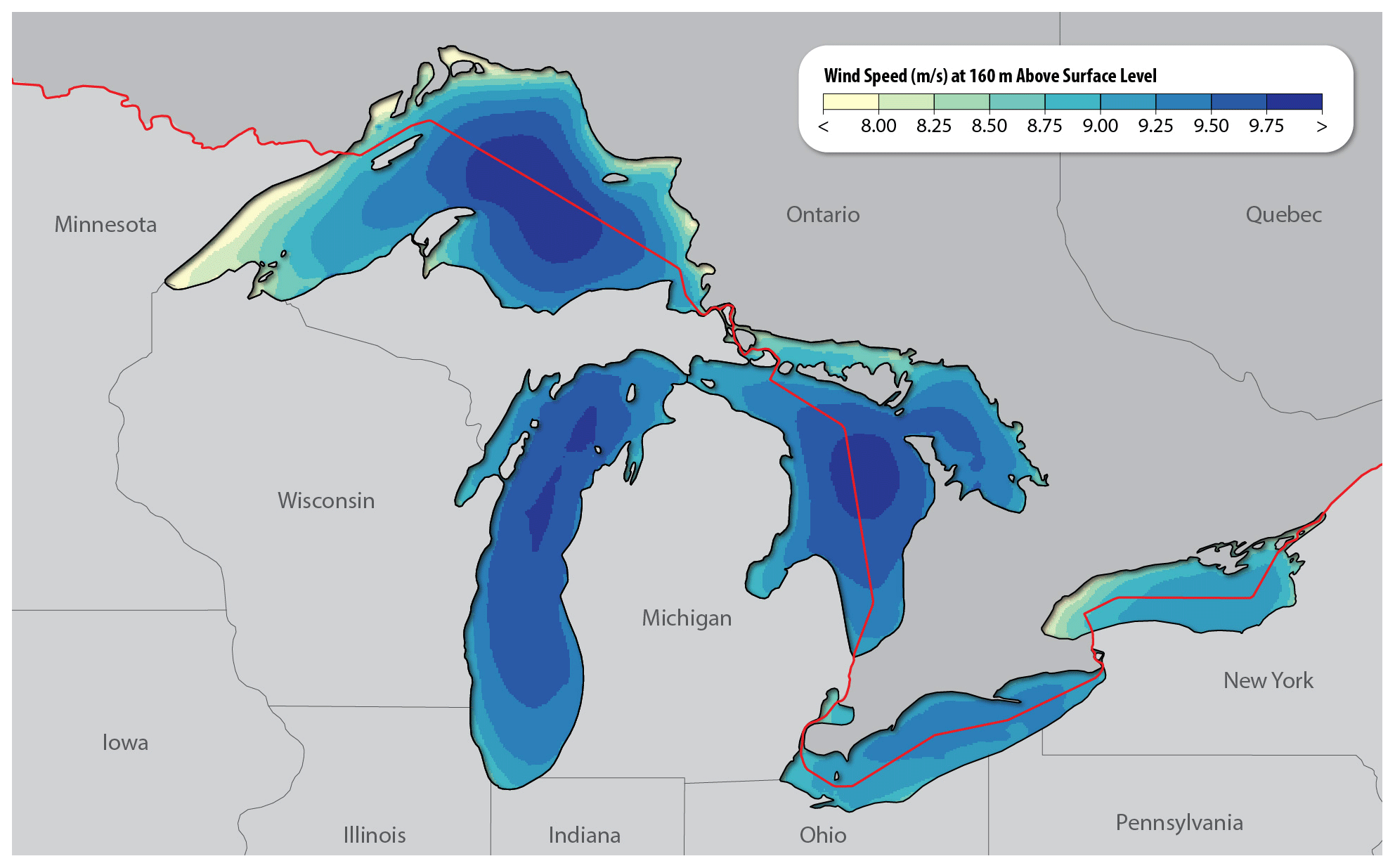
Figure 15 Map of the 21-year (2000–2020) mean wind speed at 160 m a.s.l. for the Great Lakes region. The dashed red line represents the limit of the US EEZ.

8 NOW-23 data set in the South Pacific region

The South Pacific (offshore California) was the first region to be considered for the development of this long-term wind resource data set as part of a Bureau of Ocean Energy Management (BOEM)-funded pilot project, and the development of the data set has been subject to revisions. The development of the first version of a 20-year data set for the California Outer Continental Shelf (OCS), called “CA20”, is described in Optis et al. (2020d). As detailed in the report, 16 WRF model ensemble members (Table 3) were considered by tweaking the reanalysis forcing, PBL scheme, SST product, and LSM. The WRF model setup employed for the long-term CA20 data set was selected based on a validation against available observations at that time (an array of near-surface NDBC buoys and coastal radars) and based on the validation results obtained in the Mid-Atlantic region. As a result of this validation, a 20-year data set (1 January 2000–31 December 2019) was run using the ERA5 reanalysis product, the MYNN PBL scheme, the OSTIA SST product, the Noah LSM, and the MYNN surface layer scheme.

The available measurements used to validate the CA20 model are less than ideal. In fact, the NDBC buoys only provide measurements close to the surface, which are insufficient to determine the wind resource at the relevant heights for wind energy purposes. Coastal radars provide measurements at heights of interest, but the WRF model validation at their locations becomes uncertain due to large meteorological gradients at the land–ocean interface. Also, results from the Mid-Atlantic validation cannot be directly applied to the US West Coast, given the different domain-specific processes and features that might determine a different optimal WRF model setup. When the CA20 data set was developed, the absence of floating lidar observations in the California OCS was recognized as a significant limitation to the analysis and initial validation of CA20.

Two floating lidars were deployed in the region in late 2020 – one near the Humboldt wind energy lease area in the northern part of the domain and one near the Morro Bay wind energy lease area further south (Krishnamurthy et al., 2023). The WRF model setup originally used in the CA20 data set was then run over the October 2020–September 2021 period and compared against the concurrent observations collected by the two lidars. This comparison revealed a significant bias in the CA20 modeled data, especially at the Humboldt lidar location. This bias and its impact on energy assessments in the California OCS are described in Bodini et al. (2022).

Additional analysis (Bodini et al., 2024) has shown that the choice of the PBL scheme is responsible for the vast majority of the bias in the CA20 data set. The MYNN PBL scheme overestimates the frequency of stable conditions, especially at Humboldt, resulting in reduced vertical turbulent mixing and allowing the acceleration of hub height winds, more intense low-level jets, and higher-amplitude inertial oscillations. Also, during synoptic-scale northerly flows driven by the North Pacific high and inland thermal low, simulations using the MYNN PBL scheme show a coastal warm bias in selected case studies, which contributes to the modeled wind speed bias by altering the boundary layer thermodynamics via a thermal wind mechanism. Furthermore, we found that the YSU PBL scheme strongly reduces the bias at both Humboldt and Morro Bay. Given the strong performance of the YSU-based runs in the South Pacific region, we reran the full long-term simulation in the region using the YSU PBL scheme, and this version is the one included in the NOW-23 data set. The results of this in-depth analysis, additional validation against floating lidars and coastal radars, and description of the updated data set is presented in Bodini et al. (2024). Here, we present a short summary of the main characteristics of the final NOW-23 data set for the South Pacific region for consistency with what is described for the other offshore regions in the NOW-23 data set.

For the validation of the NOW-23 data set in this region, we leveraged the two floating lidars at Humboldt and Morro Bay (Krishnamurthy et al., 2023), as well as the coastal wind profilers at McKinleyville and Bodega Bay (Fig. 2). Details about the instruments can be found in the reports that describe the validation efforts, as listed at the beginning of this section. We refer to the reports listed above for a comprehensive description of the results of the validation performed at the various stages of the development of the South Pacific data set. Here, we only include in Fig. 16 the vertical profiles of bias, cRMSE, and r for the WRF2 setup, which is chosen for the final NOW-23 data set, at the locations of the Humboldt and Morro Bay lidars. The setup shows a near-zero bias at all considered heights, which represents a great improvement compared to the bias found in the CA20 data set. Also, as done for the Mid-Atlantic and South Atlantic domains along the US East Coast, we verified that using a 1-month WRF model re-initialization period in our simulations does not impact the validation metrics as time goes by in each calendar month (figure not shown).

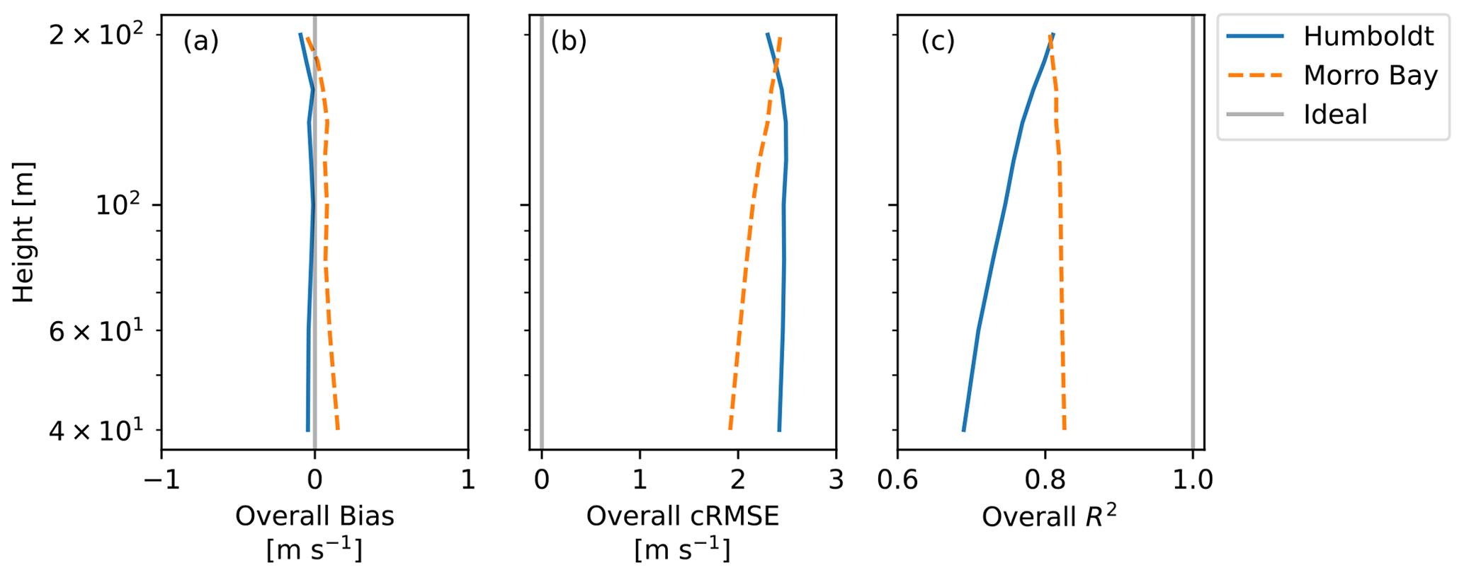
Figure 16 Vertical profiles of bias, cRMSE, and r for the WRF2 setup at the locations of the Humboldt and Morro Bay lidars calculated from October 2020 through September 2021.

Table 3 details the WRF model setup that we select and use for the NOW-23 long-term WRF model simulation in the South Pacific region, which covers the period from 1 January 2000 to 31 December 2022. The 23-year mean wind speed at 160 m a.s.l. for the South Pacific region is shown in Fig. 17, and its seasonal and diurnal variabilities are described in Appendix A. Additionally, we show in Fig. 18 the difference in mean wind speed at 160 m a.s.l. between NOW-23 (2000–2022) and the now-deprecated CA20 data set (2000–2019). We observe that NOW-23 models, on average, weaker wind speed across the whole region, with the largest difference (close to 1.5 m s⁻¹), in northern California, near the Humboldt wind energy lease area.

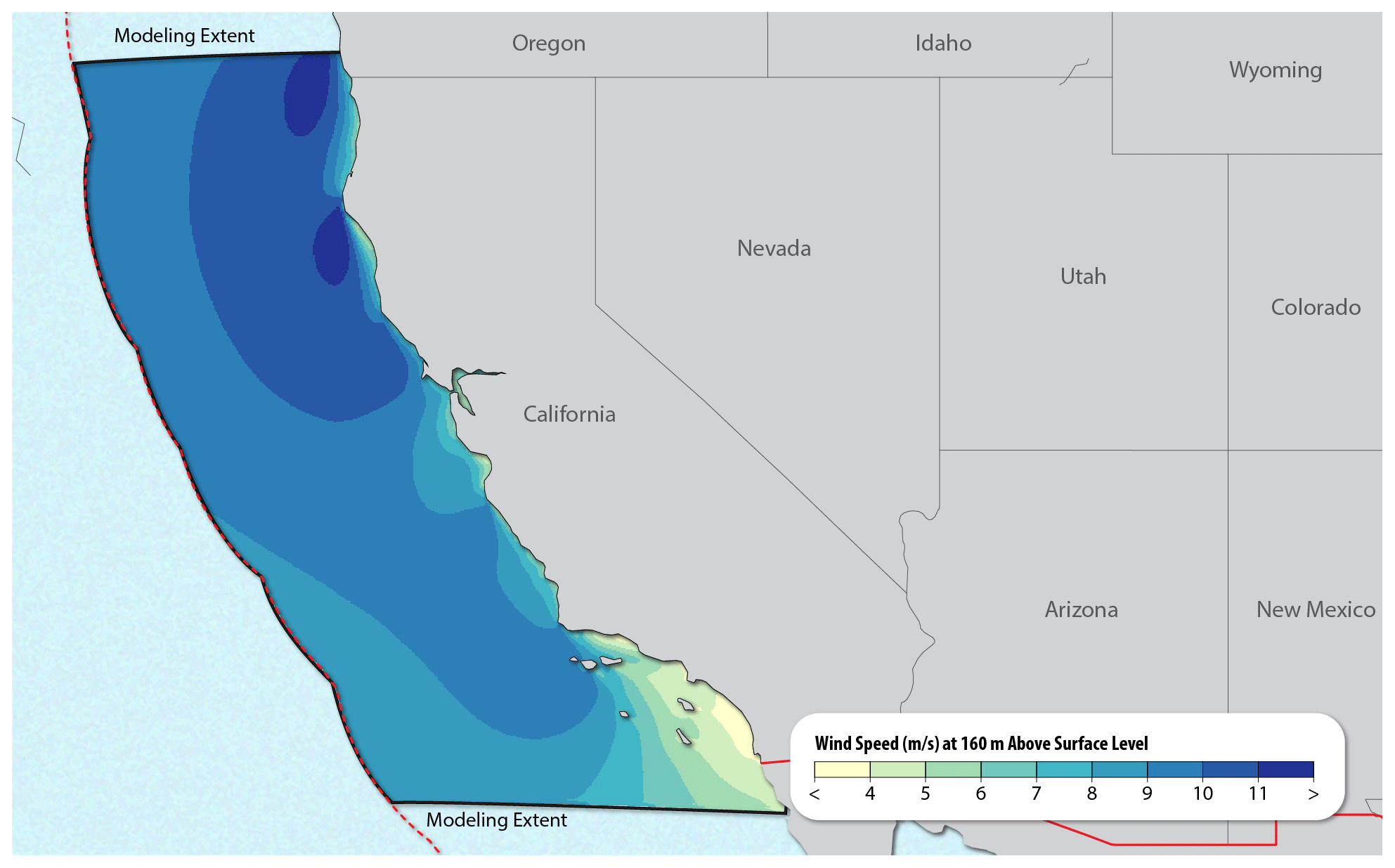
Figure 17 Map of the 22-year (2000–2022) mean wind speed at 160 m a.s.l. for the South Pacific region. The dashed red line represents the limit of the US EEZ. The continuous black line, where not overlaid with the EEZ boundary, shows the limit of the NOW-23 WRF model domain.

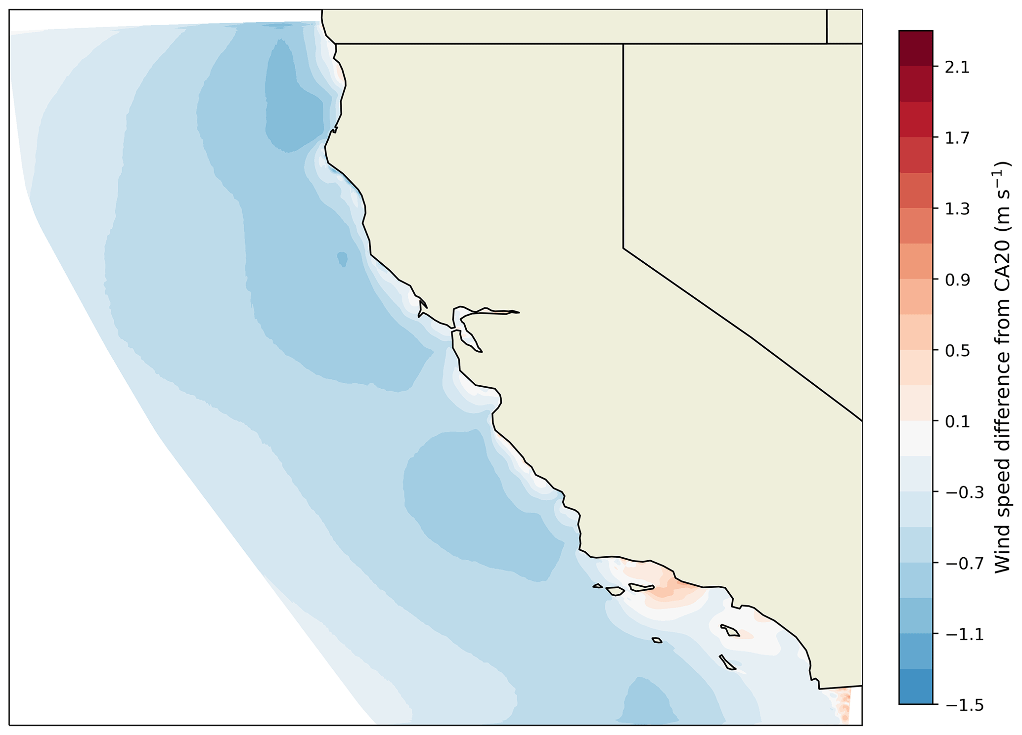
Figure 18 Map showing the difference in mean 160 m wind speed between the NOW-23 data set and the CA20 data set calculated using the full temporal extent of each data set (2000–2022 for NOW-23; 2000–2019 for CA20).

9 NOW-23 data set in the North Pacific region

No publicly available hub height offshore wind speed observations exist in the North Pacific domain. Therefore, the WRF model setup chosen for this region is based on the results obtained in the early stages of the NOW-23 development, when both the sensitivity analyses in the South Pacific (for the CA20 data set) and Mid-Atlantic domains pointed toward using a MYNN-based WRF model setup. Thus, this setup (Table 3) is selected in the North Pacific region with no additional validation against observations. In this region, NOW-23 covers the period from 1 January 2000 to 31 December 2019. The 20-year mean wind speed at 160 m a.s.l. for the North Pacific region is shown in Fig. 19.

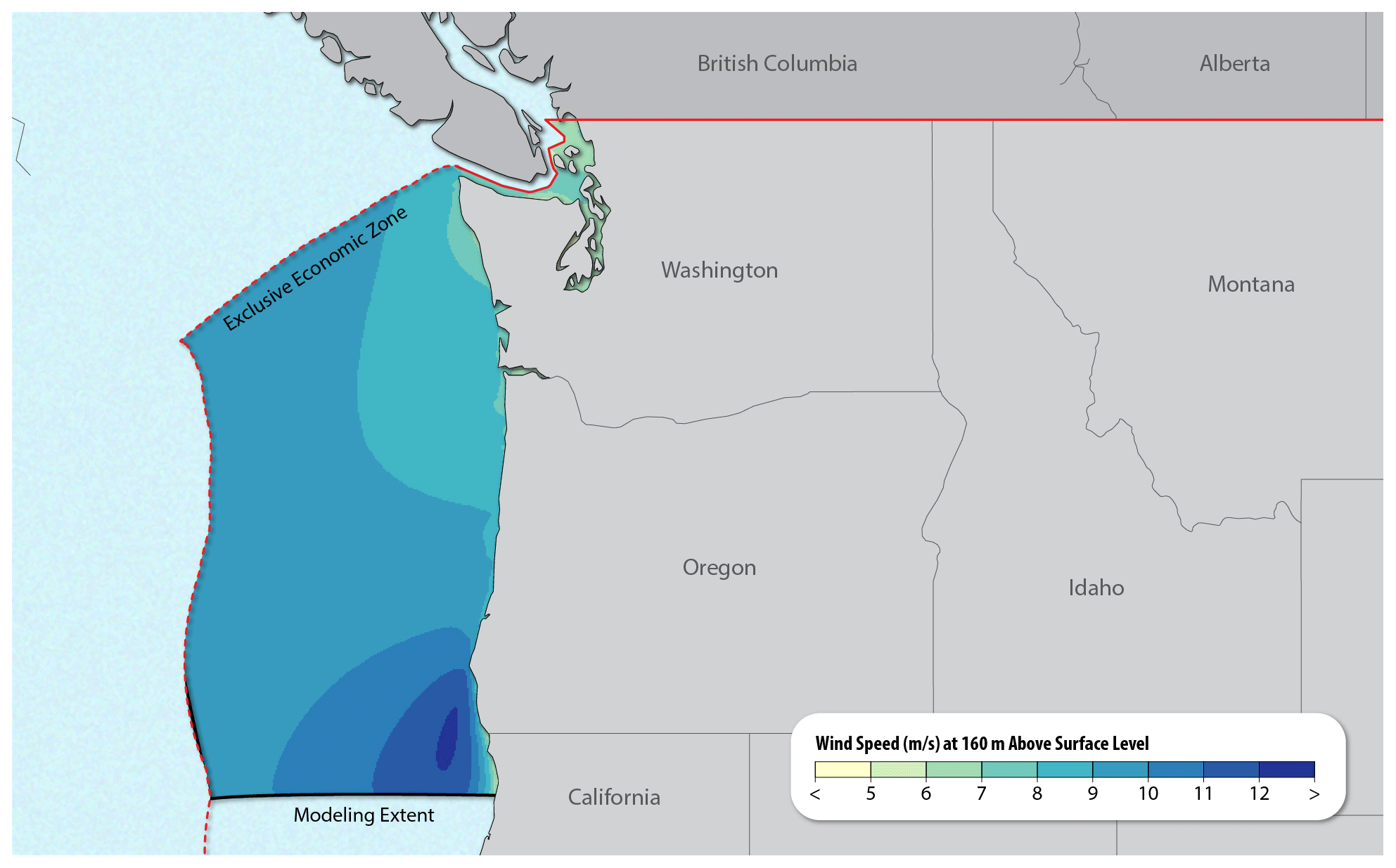
Figure 19 Map of the 20-year (2000–2019) mean wind speed at 160 m a.s.l. for the North Pacific region. The dashed red line represents the limit of the US EEZ. The continuous black line, where not overlaid with the EEZ boundary, shows the limit of the NOW-23 WRF model domain.

Because the review of the first-generation CA20 South Pacific data set, generated using the MYNN PBL parameterization, revealed a significant wind speed bias, we extend the review northward through the North Pacific coast. This preliminary examination consists of a comparison between two WRF model simulations with different physics configurations run for the year 2020. The first simulation mimics the setup of the main 20-year run for this region, and we compare that with a second simulation that uses the YSU PBL scheme and the MM5 surface layer parameterization. We find that the mean wind speed findings are consistent with those in the South Pacific data set, with stronger wind speeds off the coast resulting from the MYNN/MYNN (PBL scheme/surface layer parameterization) setup compared with that of YSU/MM5. Differences are larger (>0.5 m s⁻¹) off the southern coast of Oregon and decrease in magnitude in the northern half of the regional domain and in the open ocean.

While no hub height observations of offshore wind in the region are available, model validation can be performed using near-surface buoy data, as well as coastal observations. Leveraging available observations will be essential to assess the accuracy of the chosen WRF model setup in the region and will be subject to future work, pending funding availability. In the meantime, NREL and its project partners warrant caution for the stakeholders interested in using the NOW-23 data set in this region.

10 NOW-23 data set in Hawaii

Similar to the North Pacific region, we conduct no validation for the Hawaii domain, where no observations of hub height offshore wind were publicly available when this regional analysis was initiated at the early stages of the project. The WRF model setup used in the NOW-23 Hawaii data set is based on the results obtained in the South Pacific (for its now-deprecated CA20 data set) and the Mid-Atlantic domains. Table 3 details the WRF model setup that we select and use for the long-term WRF model simulation in the Hawaii region, which covers the period from 1 January 2000 to 31 December 2019. The 20-year mean wind speed at 160 m a.s.l. for the Hawaii region is shown in Fig. 20. We find a larger spatial variability in the mean offshore wind speed compared to the other offshore regions. In general, mean winds are stronger south of the Hawaii islands and on the northern side of the archipelago. A strong wind resource is also observed in the channel between the islands of Hawaii and Maui. Appendix A shows the variability in the long-term wind resource.

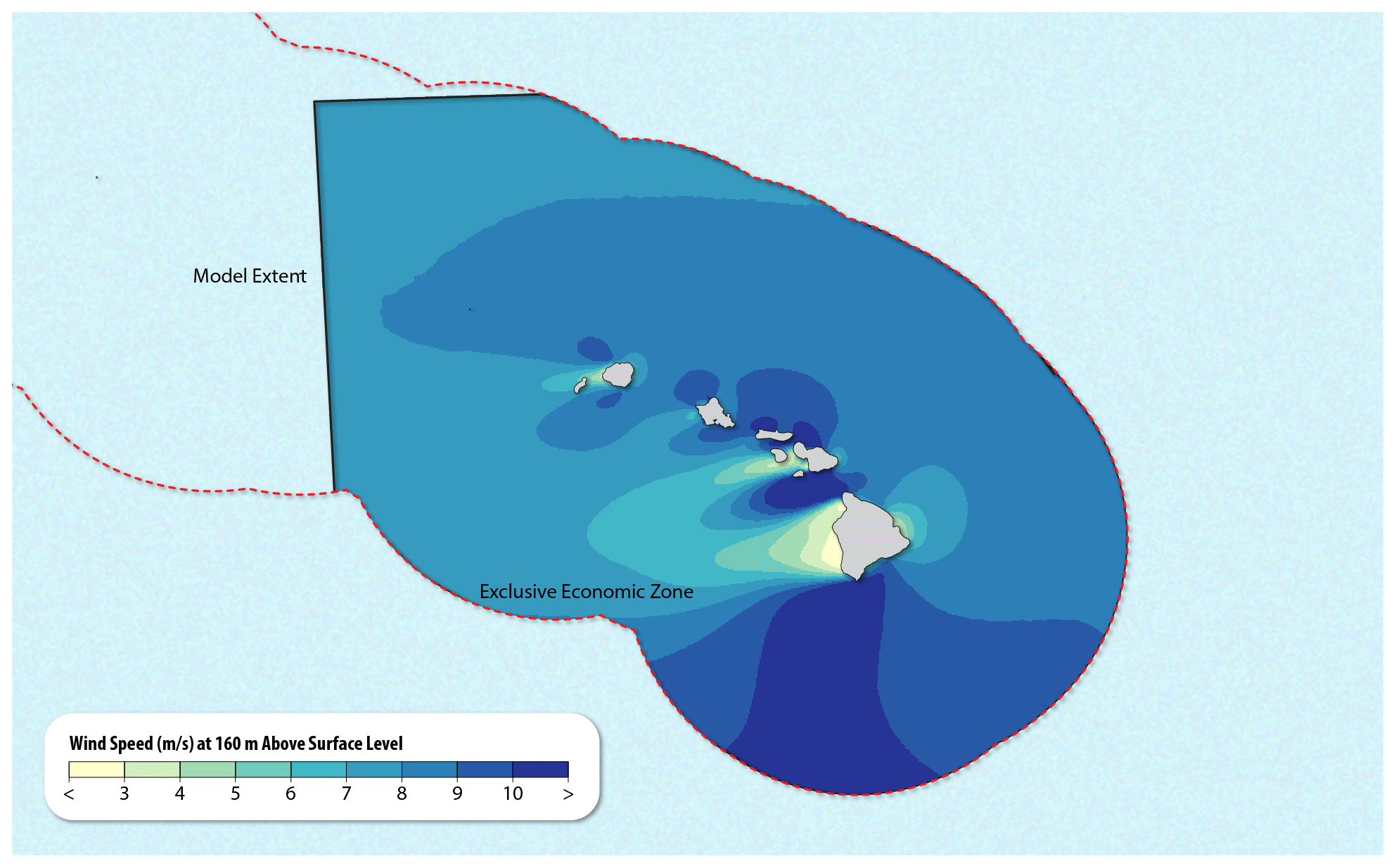
Figure 20 Map of the 20-year (2000–2019) mean wind speed at 160 m a.s.l. for the Hawaii region. The dashed red line represents the limit of the US EEZ. The continuous black line, where not overlaid with the EEZ boundary, shows the limit of the NOW-23 WRF model domain.

A floating lidar was deployed in the Hawaii region by PNNL in December 2022, and its data are publicly available. The observations collected by this instrument, together with other near-surface and onshore data sets, will be essential in assessing the accuracy of the chosen WRF model setup in the region, and will be subject to future work, pending funding availability. In the meantime, NREL warrants caution for the stakeholders interested in using this data set in this region.

11 Uncertainty quantification

NOW-23 is a modeled data set, and, as such, it comes with inherent, unavoidable uncertainty. Ideally, a modeled data set would come with full uncertainty information so that each user can make informed decisions on whether the level of uncertainty in a given region is acceptable for their specific application. As part of the NOW-23 development, significant effort was undertaken to provide stakeholders with this uncertainty information. We tackle this aspect from different points of view which are briefly summarized in the next paragraphs. For each topic listed below, we refer to other peer-reviewed publications for a detailed description of the analyses performed.

11.1 Ensemble-based uncertainty

First, we focus on the characterization of what we call the ensemble-based uncertainty, or boundary condition and parametric uncertainty, in modeled wind speed. When considering NWP models, the choices of the model setup and inputs have a direct impact on the model wind speed prediction and therefore on its uncertainty. Estimating the boundary condition and parametric uncertainty associated with modeled wind speed requires running a model ensemble which can be computationally intensive for producing long-term data over large regions as for the NOW-23 data set. Therefore, we propose two alternative approaches that use a short-term mesoscale ensemble (i.e., the 1-year WRF model ensemble we use for model setup selection in several offshore regions) alongside a single model run for the desired long-term period (i.e., the 20+-year NOW-23 run). We quantify hub height wind speed boundary condition and parametric uncertainty from the short-term model ensemble as its normalized across-ensemble standard deviation. Then, we use a gradient-boosting model and an analog ensemble approach to extrapolate the uncertainty to the full 20+-year period.

We test our proposed methods in the South Pacific domain (using the now-deprecated MYNN-based CA20 data set) and find that both approaches provide accurate estimates of long-term wind speed boundary condition and parametric uncertainty (r²>0.75), with the gradient-boosting model performing slightly better than the analog ensemble. We also assess the physical variability in the uncertainty estimates and find that wind speed uncertainty increases closer to land, stable and unstable cases have larger uncertainty than neutral conditions, and winter has a smaller boundary condition and parametric sensitivity than summer. Finally, we report a median hourly uncertainty between 10 % and 14 % of the mean 100 m wind speed values across the offshore wind energy lease areas in the region. The results of this analysis are described in detail in Bodini et al. (2021).

11.2 Model uncertainty compared to observations

While helpful from a modeling point of view, the assessment of the boundary condition and parametric uncertainty presents several limitations. In fact, the magnitude of this ensemble-based uncertainty is strictly connected to the (limited) number of choices sampled within the considered model setups so that only a limited component of the actual wind speed error with respect to observations (our best proxy for the true wind speed) can be quantified from it. The full uncertainty in NWP-model-predicted wind speed can be quantified only when direct observations of the wind resource are available. In this scenario, the residuals between modeled and observed wind speed can be calculated, and the model error is quantified in terms of its bias (i.e., the mean of the residuals) and uncertainty (i.e., the standard deviation of the residuals). The obtained model uncertainty would then be added to the inherent uncertainty in the wind speed measurements.

We apply this approach in the Mid-Atlantic region. Given the lack of long-term (20+-year) hub height offshore wind speed observations in the region (the same applies to all the US offshore regions), we propose a methodological framework to leverage both floating lidar and near-surface buoy observations to quantify uncertainty in the long-term modeled hub height wind resource. We train and validate a machine learning technique to vertically extrapolate near-surface wind speed to hub height using the available short-term lidar data sets in the region. We then apply this model to vertically extrapolate the long-term near-surface buoy wind speed observations to hub height for comparison to the long-term NOW-23 data set. Using this comprehensive approach, we find that the mean 20-year uncertainty (including the uncertainty coming from the observations and from the application of the machine learning approach) in 140 m wind speed is slightly lower than 3 m s⁻¹ across the considered region, with larger uncertainty in stable conditions. The results of this analysis are described in detail in Bodini et al. (2023).

12 NOW-WAKES: a post-construction data set for the Mid-Atlantic wind energy areas

A promising offshore wind resource is often located near large population centers so that a rapid wind plant development is expected. However, wind turbines and wind plants generate wakes, which are regions of reduced wind speed that may negatively impact downwind turbines and plants. As part of the NOW-23 data set, we developed NOW-WAKES, a 1-year post-construction data set to model and assess the impact of offshore wakes from the upcoming wind plants in some of the lease and call areas (as of 2019) in the Mid-Atlantic region. We use WRF model and its Fitch wind farm parameterization (Fitch et al., 2012) to calculate wake effects and distinguish between wakes generated within one plant and those generated externally between plants. The strongest wakes, propagating 55 km, occur during stable stratification in summer, which coincides with peak grid demand in New England. The mean year-long wake impacts reduce power output by roughly 35 %, with internal wakes causing greater power losses (27 % on average) than external wakes (14 % on average). The results of this analysis are described in detail in Rosencrans et al. (2023).

As part of the NOW-WAKES effort, we also investigate the uncertainty connected to some of the modeling choices made in this 1-year analysis using two different PBL schemes for these simulations, namely the MYNN PBL scheme and the new National Center for Atmospheric Research (NCAR) 3DPBL scheme (Kosović et al., 2020; Juliano et al., 2022). The average losses in hub height wind speeds within an ideal plant differ between the two schemes by up to −0.20 to 0.22 m s⁻¹, and correspondingly, capacity factors range from 39.5 % to 53.8 %. These results suggest that the choice of the PBL scheme can also contribute to uncertainty in modeled wakes, and therefore we recommend including PBL variability in wind plant planning sensitivity and forecasting studies. The results of this analysis are described in detail in Rybchuk et al. (2022).

Viselli et al. (2022)

Table 5 Data availability for the observational data sets used for NOW-23 validation.

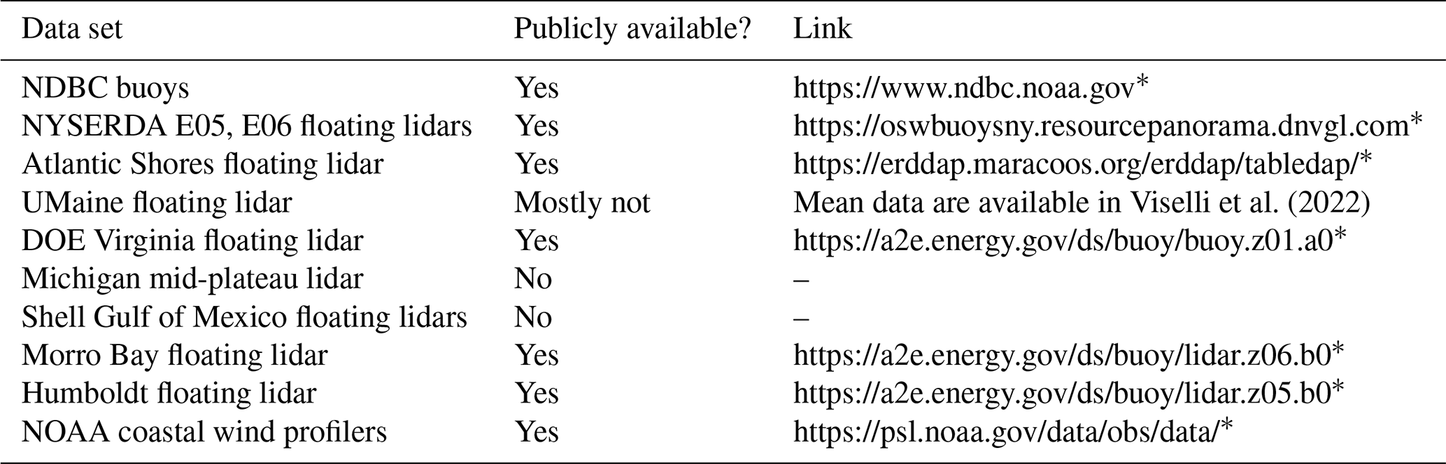
^* Last access: 22 April 2024.

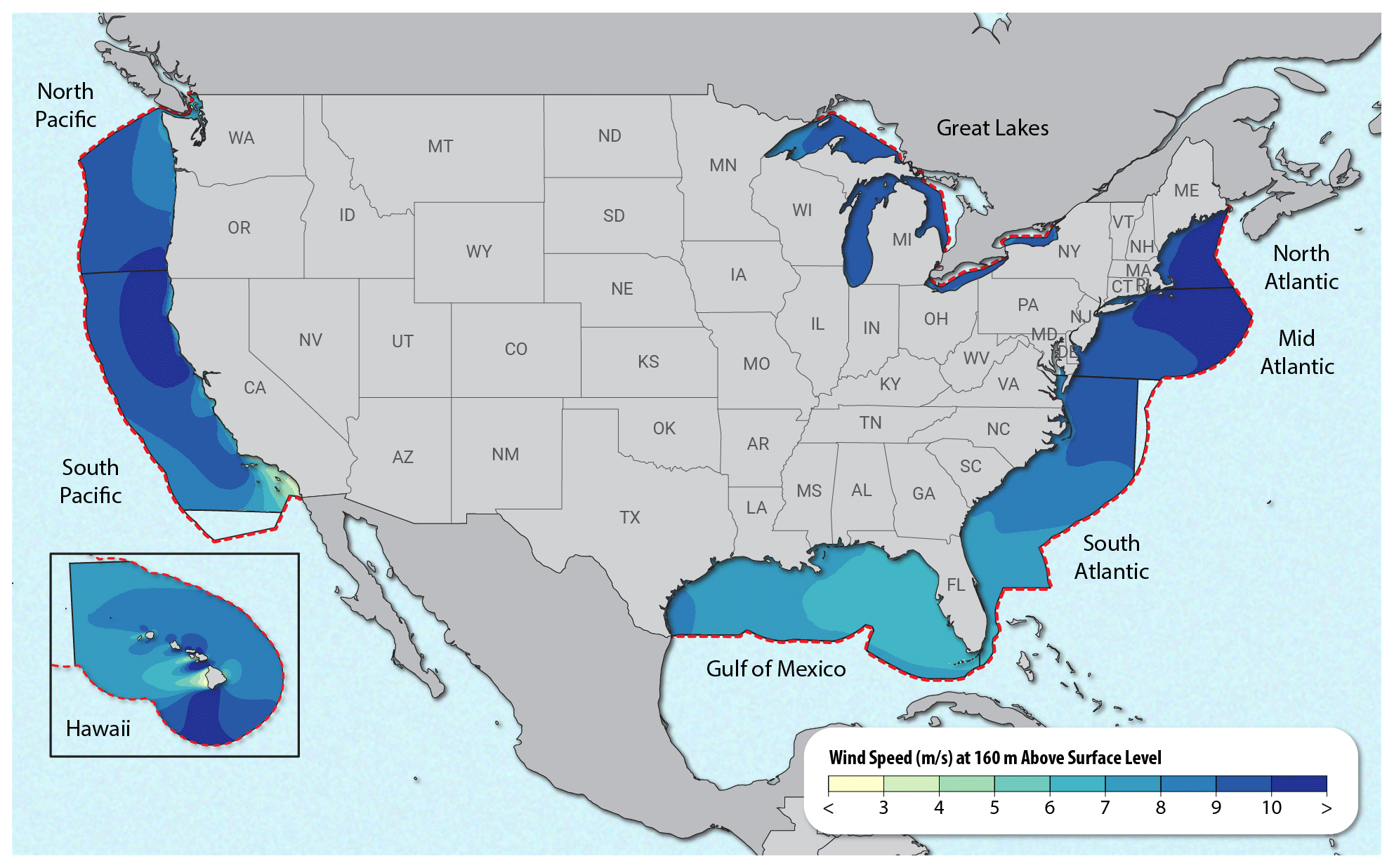
Figure 21 Mean long-term wind speed at 160 m from the NOW-23 data set for all US offshore regions (except for Alaska). The dashed red lines represent the limit of the US EEZ. The continuous black lines show where data from the regional domains were cut to create this national-scale map.

13 Code and data availability

The whole NOW-23 data set is publicly available at no cost through Amazon Web Services (AWS) at https://doi.org/10.25984/1821404 (Bodini et al., 2020). The data are stored as both HDF5 and WRG files. The same page also includes a link to the NOW-23 WRF model namelists.

The HDF5 files are available for each offshore region at both 5 min resolution and as hourly averages. The following variables are available in the HDF5 files:

• wind speed at 10 and 20 m intervals between 20 and 300, 400, and 500 m (m s⁻¹);

• wind direction at 10 and 20 m intervals between 20 and 300, 400, and 500 m (° from N);

• planetary boundary layer height (m);

• pressure at 0, 100, 200, and 300 m (Pa);

• temperature at 2, 10, and 20 m intervals between 20 and 300, 400, and 500 m (°C);

• friction velocity at 2 m (m s⁻¹);

• surface heat flux (W m⁻²);

• inverse Monin–Obukhov length at 2 m (m⁻¹);

• sea surface temperature (°C);

• skin temperature (°C);

• relative humidity at 2 m (%); and

• roughness length (m).

To facilitate accessing, extracting, and manipulating data from the NOW-23 large files, NREL has developed the REsource eXtraction (rex) tool. Instructions on how to install rex, as well as examples of its usage, can be found at https://nrel.github.io/rex (last access: 25 April 2024; DOI: https://doi.org/10.5281/zenodo.4499033, Rossol and Buster, 2021​​​​​​). We note that rex allows, among others, the extraction of a subset of variables over a single location, a customized region, and an automatic interpolation of the wind speed data to an arbitrary height.

The WRG file format is an industry standard format for publishing modeled wind resource data sets. In general, WRG files provide wind rose information at a specific height at each modeled grid cell. This information is specified in a WRG by providing Weibull fit parameters for reported wind speeds in a given sector. Considerable information is lost when pivoting to a WRG from the HDF5 format. Specifically, all temporal information (e.g., seasonal and diurnal trends) and other relevant atmospheric parameters are discarded, with only wind speed and direction being preserved. Regardless, the WRG format has been the industry standard for decades and is still actively used for offshore wind resource assessment. For the NOW-23 data sets, NREL has provided WRG files calculated at 160 m and at 30° wind direction sector bins. An open-source codebase has also been publicly released (https://github.com/NREL/wrg_maker, last access: 25 April 2024; DOI: https://doi.org/10.5281/zenodo.11040122, Optis and Bodini, 2024) so that stakeholders can produce additional WRG files from the NOW-23 data set if desired.

To further facilitate access to the NOW-23 data, Bodini et al. (2020) also includes sample data (in an easily accessible .csv format) at the locations of the lidars used to validate the NOW-23 data set (locations in Fig. 2).

The NOW-23 data set can also be visualized and accessed through NREL's Wind Resource Database (https://wrdb.nrel.gov/, National Renewable Energy Laboratory, 2024). Any request for technical support on the NOW-23 data set can be directed to wrdb@nrel.gov.

Some of the observations used for model validation are also publicly available. Details about the observational data sets used are included in Table 5.

14 Conclusions

The NOW-23 data set is a cutting-edge, offshore-focused wind resource assessment data set that aims to support the growth of the offshore wind energy sector in the United States. This comprehensive overview paper outlines the approach employed to generate and validate the data set for each US offshore region (with the exception of Alaska). The national mean long-term wind speed, depicted in Fig. 21, is derived by amalgamating all the regional domains.

Anticipated to replace NREL's WIND Toolkit and become one of the most widely utilized data sets for offshore wind resource assessment in the United States, the NOW-23 data set showcases the significance of conducting regionally focused validation and selecting appropriate model setups based on multiple observational data sets. The analysis underscores the symbiotic relationship between NWP models and observations, emphasizing their interconnectedness. To mitigate the inherent uncertainty in numerical models, an increased quantity of long-term observations is required, which can be facilitated through the sharing of proprietary observational data sets. In assessing the costs and benefits of data-sharing initiatives, it is essential for stakeholders to consider the long-term advantages that the access to additional observational data sets can offer in terms of enhanced numerical modeling.

Further analysis and validation are needed for the NOW-23 data set in Hawaii and the North Pacific, subject to future work contingent on funding availability. As more offshore observations become accessible, the current validation efforts can be expanded to ensure the NOW-23 model setup is validated in regions of interest for present and future offshore wind energy lease areas. Additionally, regular updates to the NOW-23 data set (pending funding availability) are desirable, enabling stakeholders to employ the industry standard measure–correlate–predict approach as they collect short-term observations in the future. Also, an analysis similar to what was done to create NOW-WAKES can be replicated in different offshore regions. As offshore wind turbines are built in the US, the simulated wake effects can and should be validated against any available observations. Last, given the unsatisfactory performance of the MYNN PBL scheme on the US West Coast, further analysis is warranted to investigate the causes of its failure in the region and propose and implement offshore-focused improvements to the parameterization scheme.

Appendix A: Seasonal and diurnal variability in long-term offshore wind speed in the NOW-23 data set

In all offshore regions modeled in NOW-23, we observe distinct seasonal and diurnal patterns in hub height wind speed.

On the US East Coast, we observe consistent seasonal and diurnal cycles in hub height wind speed. During the winter months, winds are at their strongest, gradually weakening as we move into summer. The seasonal differences in wind speed become more pronounced further offshore. A comparison of the month of January, which typically experiences the highest average wind speed, with August, when wind speed is at its lowest, reveals differences sometimes exceeding 6 m s⁻¹ (Figs. A1, A3, and A5). Additionally, a diurnal cycle is evident, with variations closer to the shore being more pronounced, likely because of sea breeze effects. In the evenings, we observe stronger winds, while the morning hours tend to have weaker wind speeds (Figs. A2, A4, and A6).

We find similar results in the Gulf region, where winter months have the strongest winds, and summer months have the weakest wind speeds. The area with the largest deviation from the annual mean varies throughout the year, with the eastern side of the Gulf experiencing the largest deviation in early winter and the western side experiencing it later in the season. A similar transition occurs from east to west during the summer months (Fig. A7). On a diurnal basis, we observe stronger winds at night and weaker winds during the day, with the most significant deviations once again near the coast (Fig. A8).

When considering the Great Lakes region, we observe the same seasonal and diurnal cycles in hub height wind speed as on the US East Coast; the strongest winds occur in winter and early spring, while the weakest winds occur in summer, with greater seasonal differences in lakes more to the south (Fig. A9). The diurnal cycle in this region is slightly delayed compared to the US East Coast, with stronger winds in the late evening and weaker winds around midnight (Fig. A10).

In the North Pacific, we find consistent seasonal and diurnal cycles in hub height wind speed. Once again, winter months have the strongest winds, while summer months have the weakest winds, except for the southern part of the ocean west of the Oregon coast where the annual cycle is opposite (Fig. A11). On a diurnal basis, we observe stronger winds in the afternoon and early night, and weaker winds in the late nights and early mornings, with the largest deviations near the coast (Fig. A12).

In the South Pacific, a different annual cycle emerges (Fig. A13) with strongest winds observed in the spring and early summer, with the southern portion of the domain experiencing stronger winds earlier than northern California. On a diurnal basis, we find similar results to what was observed in the adjacent North Pacific region, with stronger winds in the afternoon and early night (Fig. A14).

For Hawaii, the seasonal and diurnal cycles in hub height wind speed are not as clear as in the other offshore regions. Winds close to the islands are stronger in the summer and weaker in the winter. Further offshore, the seasonal variability becomes less clear (Fig. A11). On a diurnal basis, we find stronger winds closer to the islands in the afternoon and early night, and weaker winds in the late night and early morning, with the largest deviations near the coast (Fig. A16).

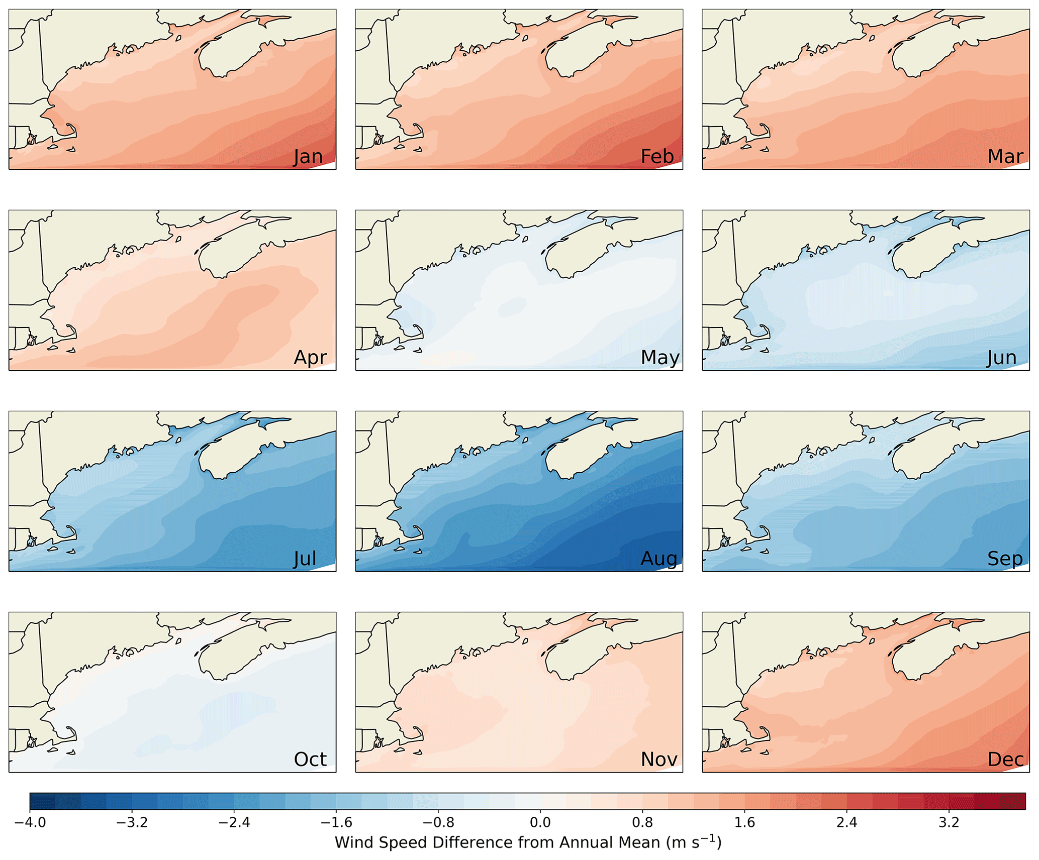
Figure A1 Maps showing the annual cycle in 160 m wind speed expressed in terms of the difference for each month's mean wind speed from the overall mean for the North Atlantic region.

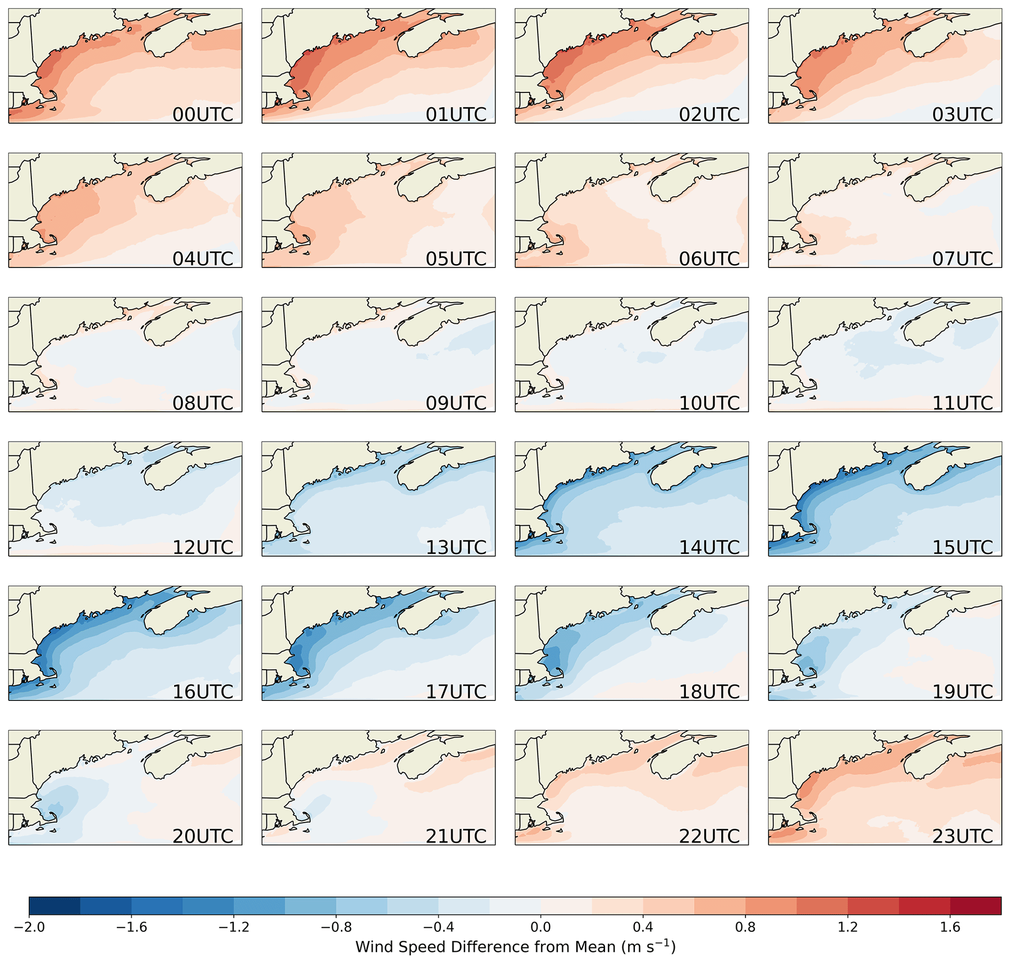
Figure A2 Maps showing the diurnal cycle in 160 m wind speed expressed in terms of the difference for each (UTC) hour's mean wind speed from the overall mean for the North Atlantic region.

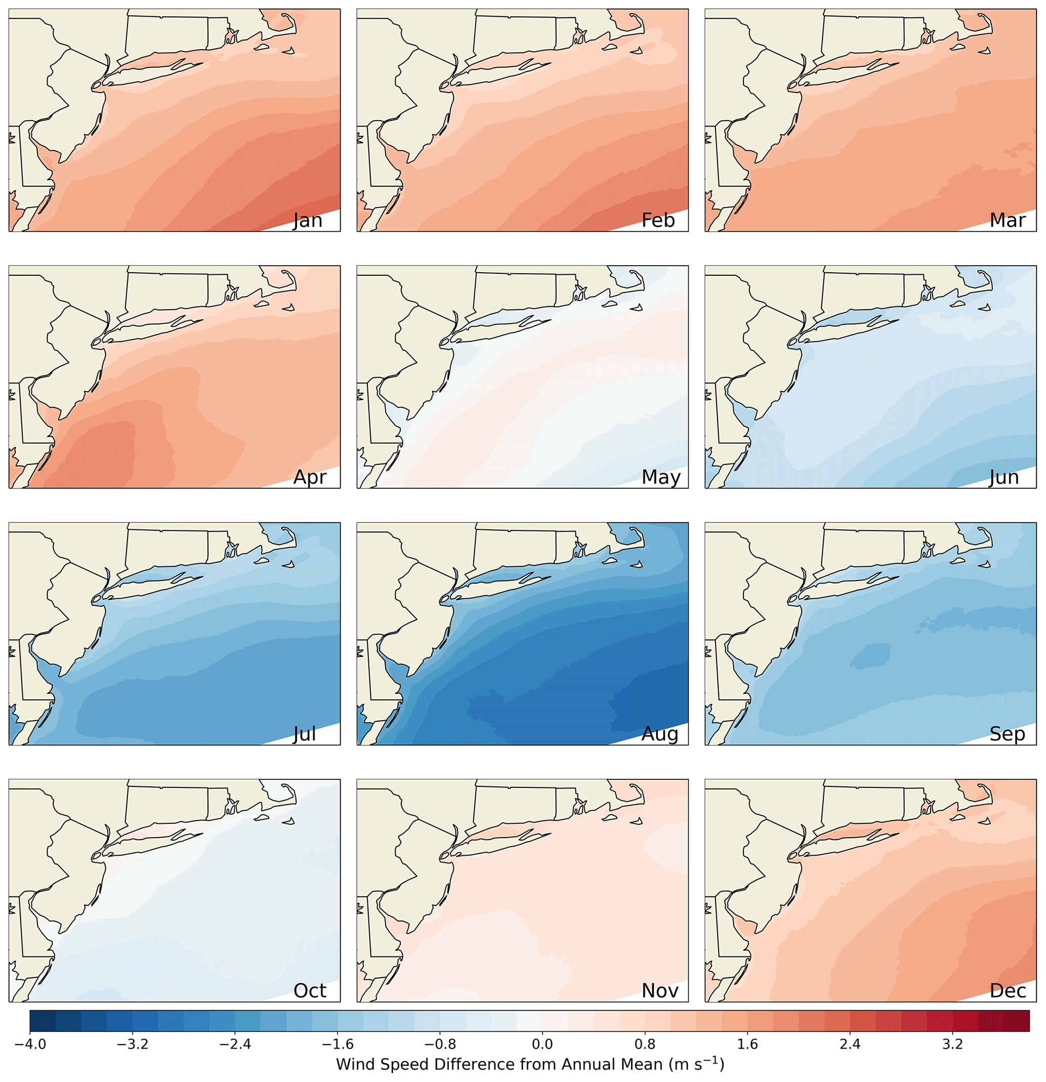
Figure A3 Maps showing the annual cycle in 160 m wind speed expressed in terms of the difference for each month's mean wind speed from the overall mean for the Mid-Atlantic region.

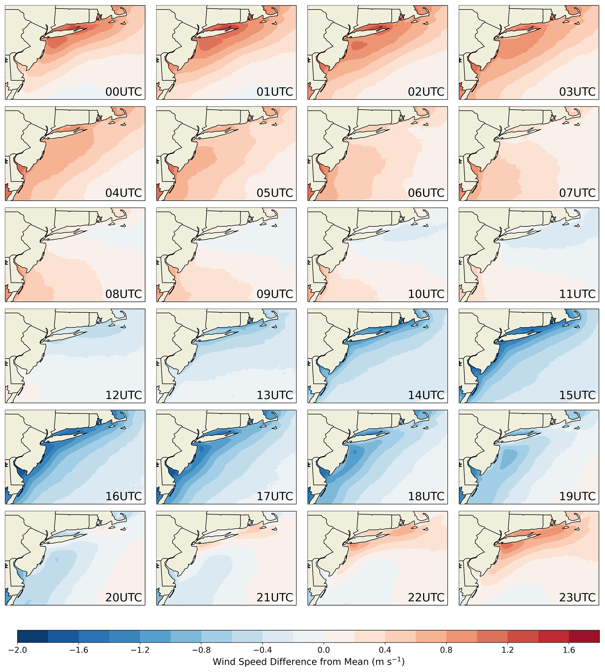
Figure A4 Maps showing the diurnal cycle in 160 m wind speed expressed in terms of the difference for each (UTC) hour's mean wind speed from the overall mean for the Mid-Atlantic region.

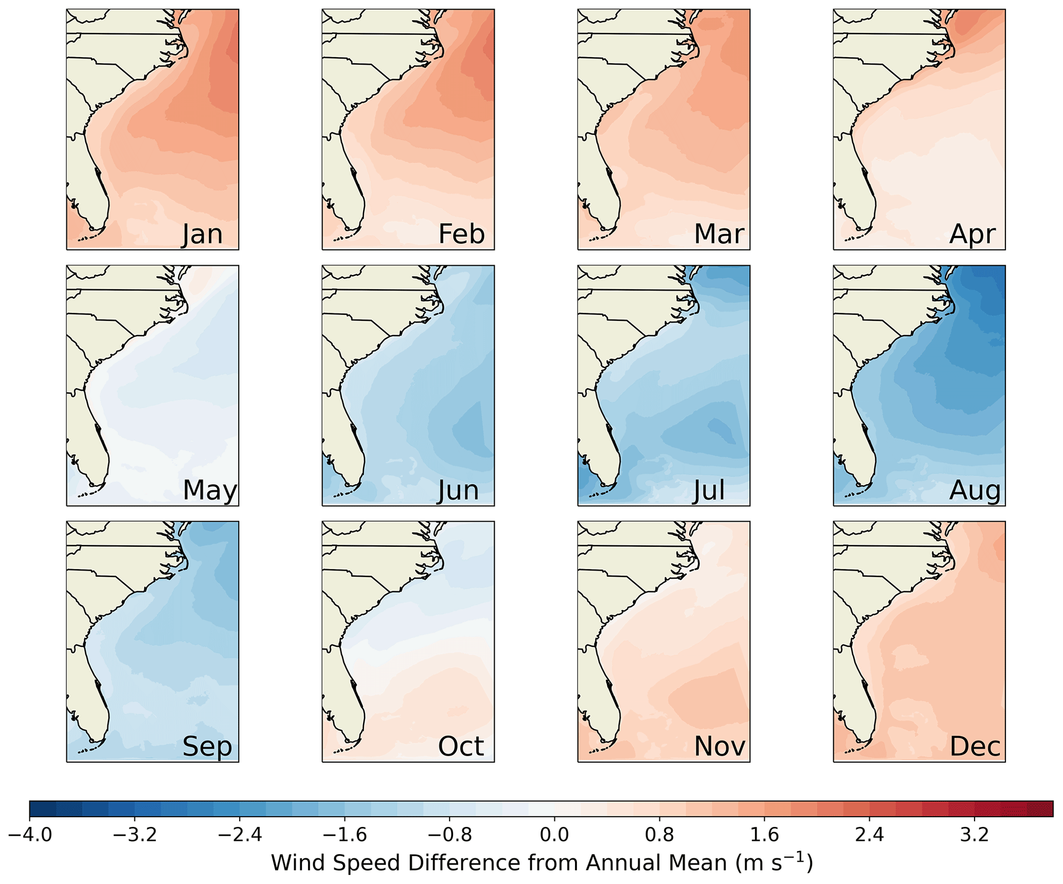
Figure A5 Maps showing the annual cycle in 160 m wind speed expressed in terms of the difference for each month's mean wind speed from the overall mean for the South Atlantic region.

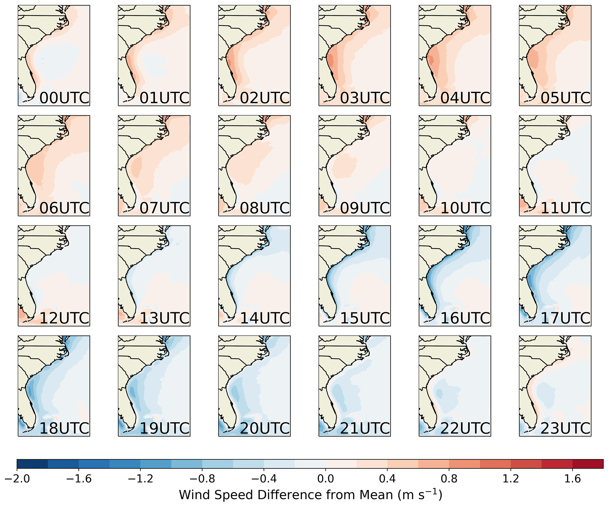
Figure A6 Maps showing the diurnal cycle in 160 m wind speed expressed in terms of the difference for each (UTC) hour's mean wind speed from the overall mean for the South Atlantic region.

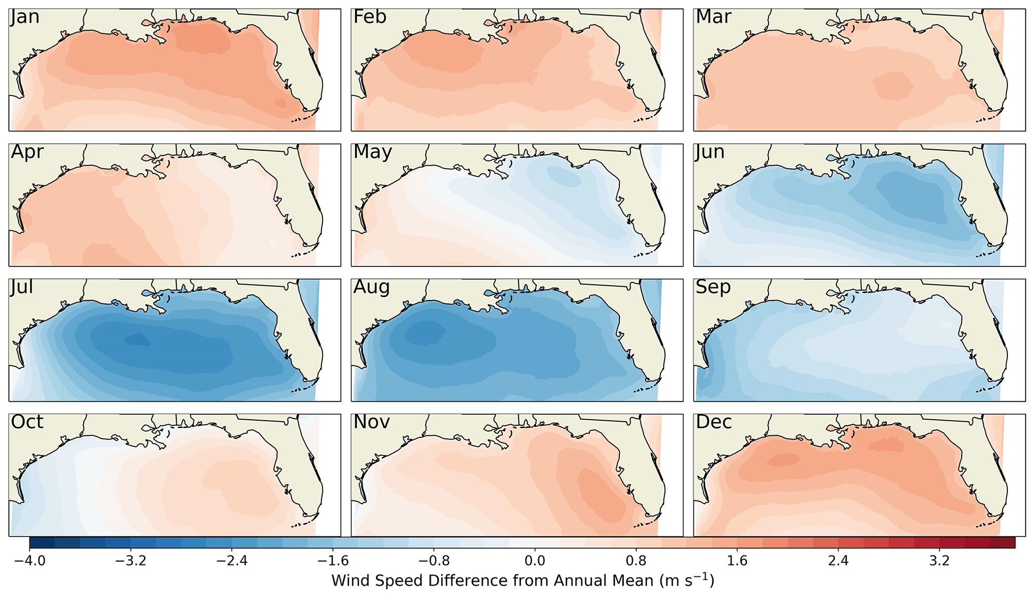
Figure A7 Maps showing the annual cycle in 160 m wind speed expressed in terms of the difference for each month's mean wind speed from the overall mean for the Gulf of Mexico region.

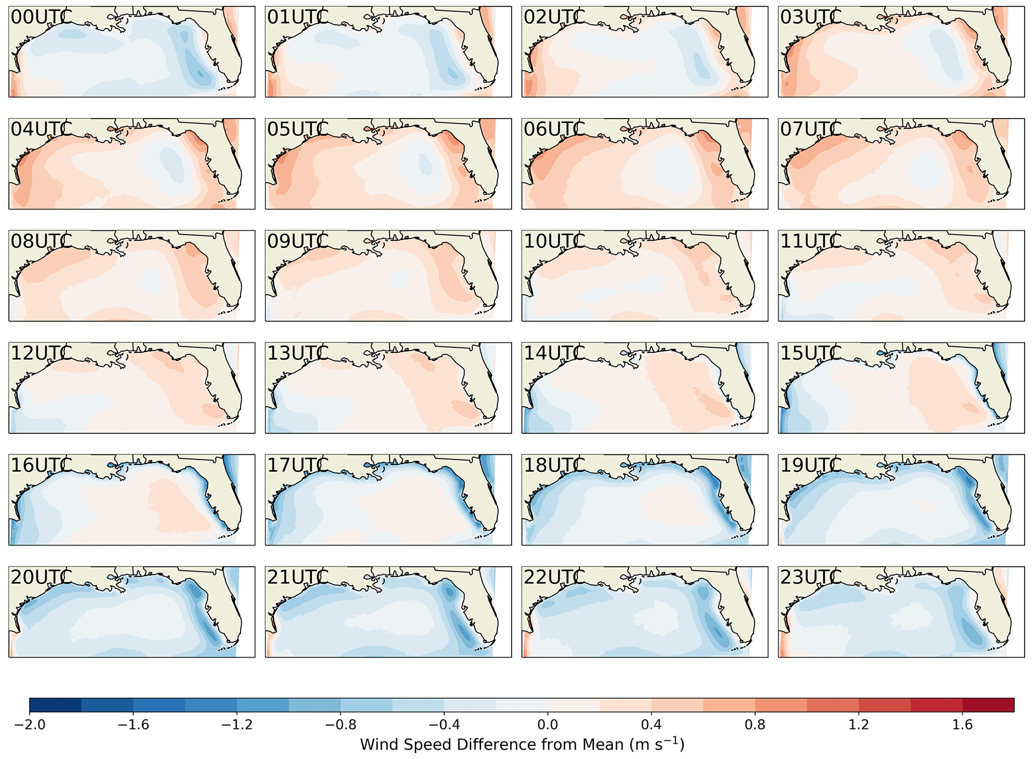
Figure A8 Maps showing the diurnal cycle in 160 m wind speed expressed in terms of the difference for each (UTC) hour's mean wind speed from the overall mean for the Gulf of Mexico region.

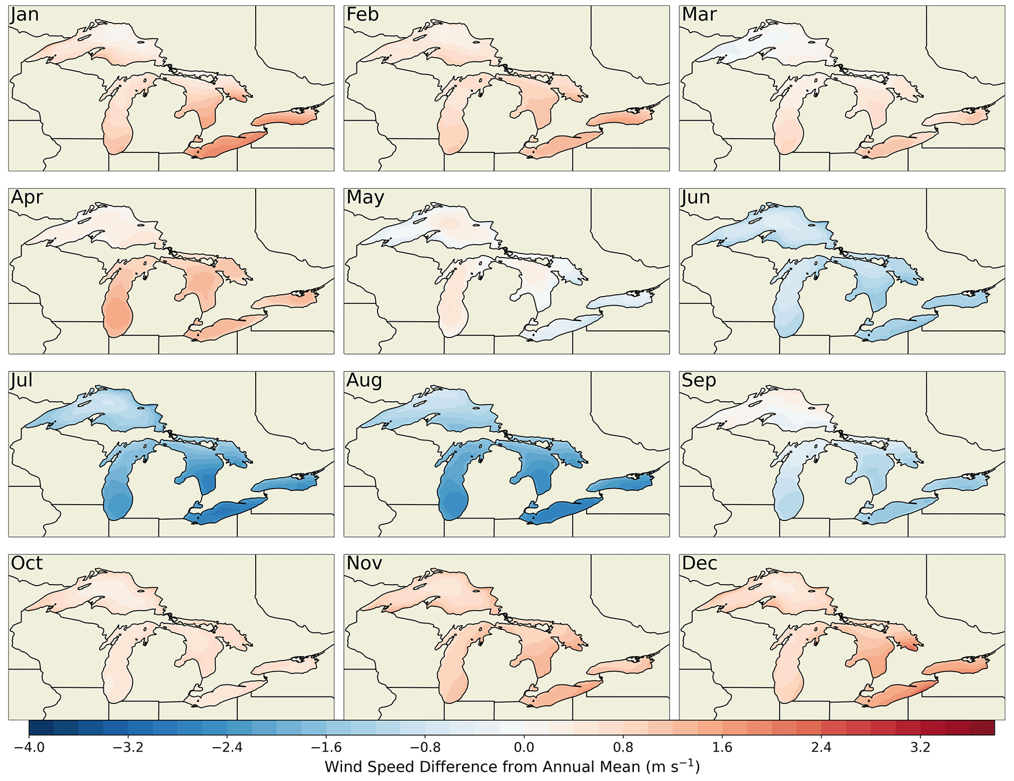
Figure A9 Maps showing the annual cycle in 160 m wind speed expressed in terms of the difference for each month's mean wind speed from the overall mean for the Great Lakes region.

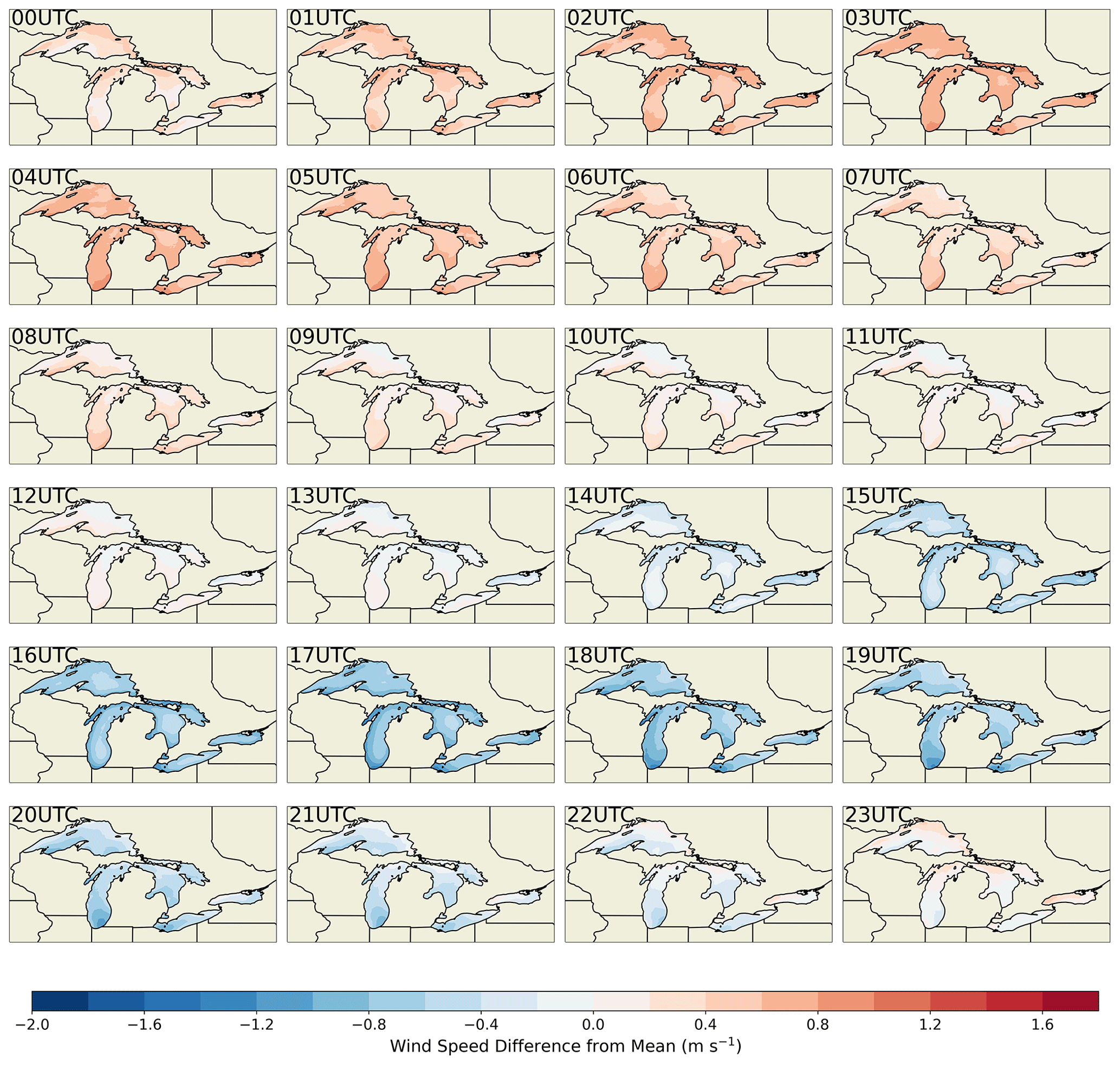
Figure A10 Maps showing the diurnal cycle in 160 m wind speed expressed in terms of the difference for each (UTC) hour's mean wind speed from the overall mean for the Great Lakes region.

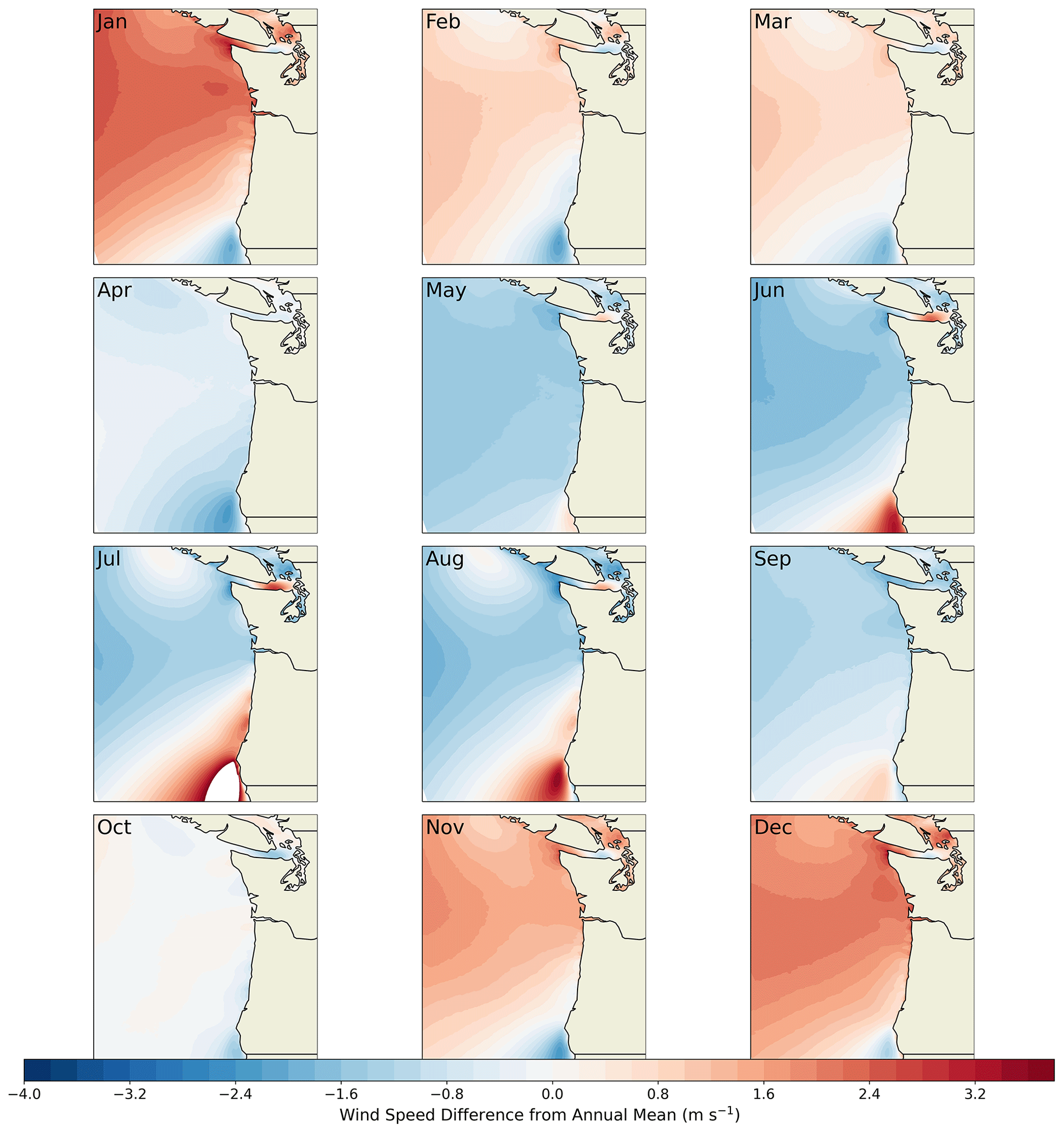
Figure A11 Maps showing the annual cycle in 160 m wind speed expressed in terms of the difference for each month's mean wind speed from the overall mean for the North Pacific region.

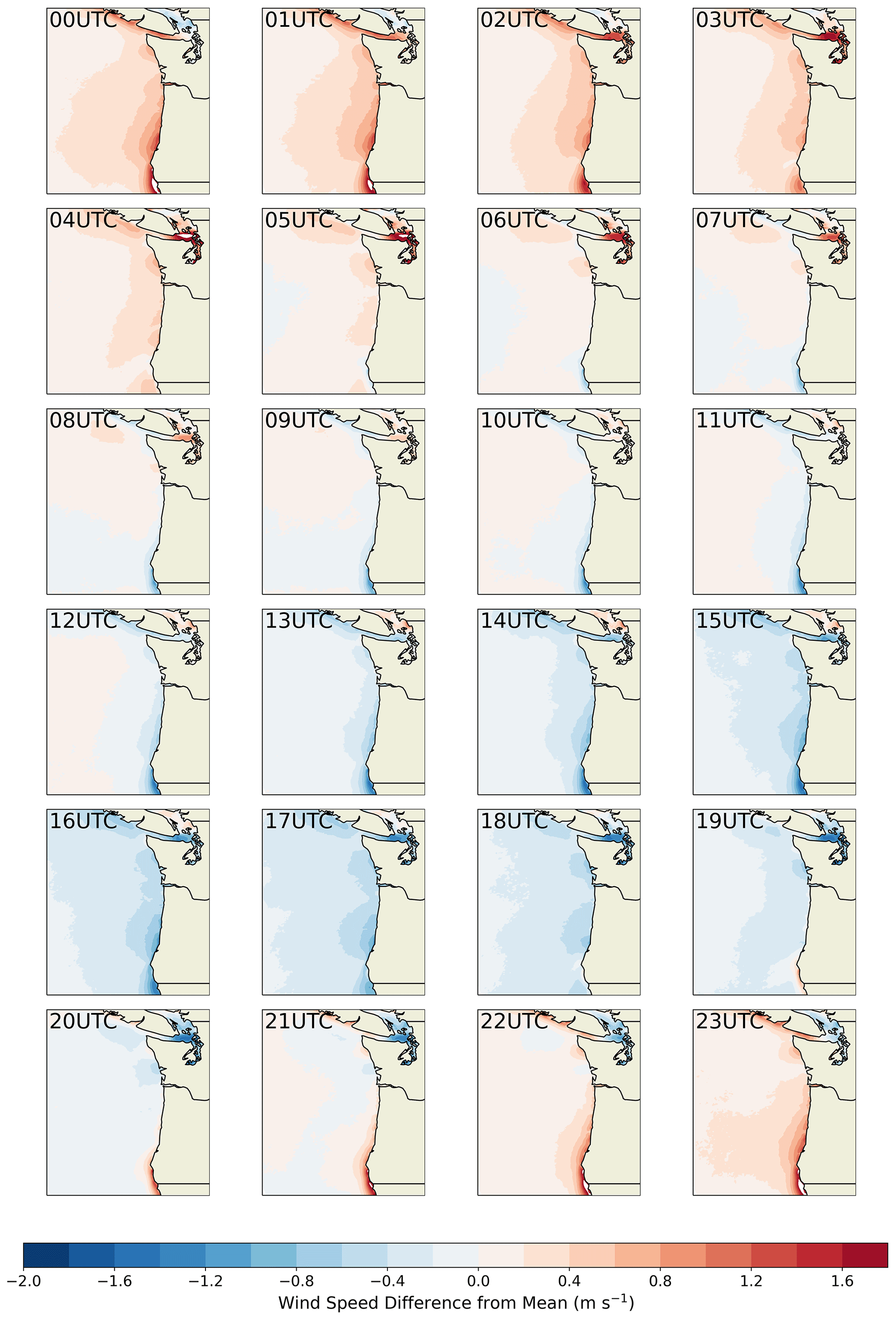
Figure A12 Maps showing the diurnal cycle in 160 m wind speed expressed in terms of the difference for each (UTC) hour's mean wind speed from the overall mean for the North Pacific region.

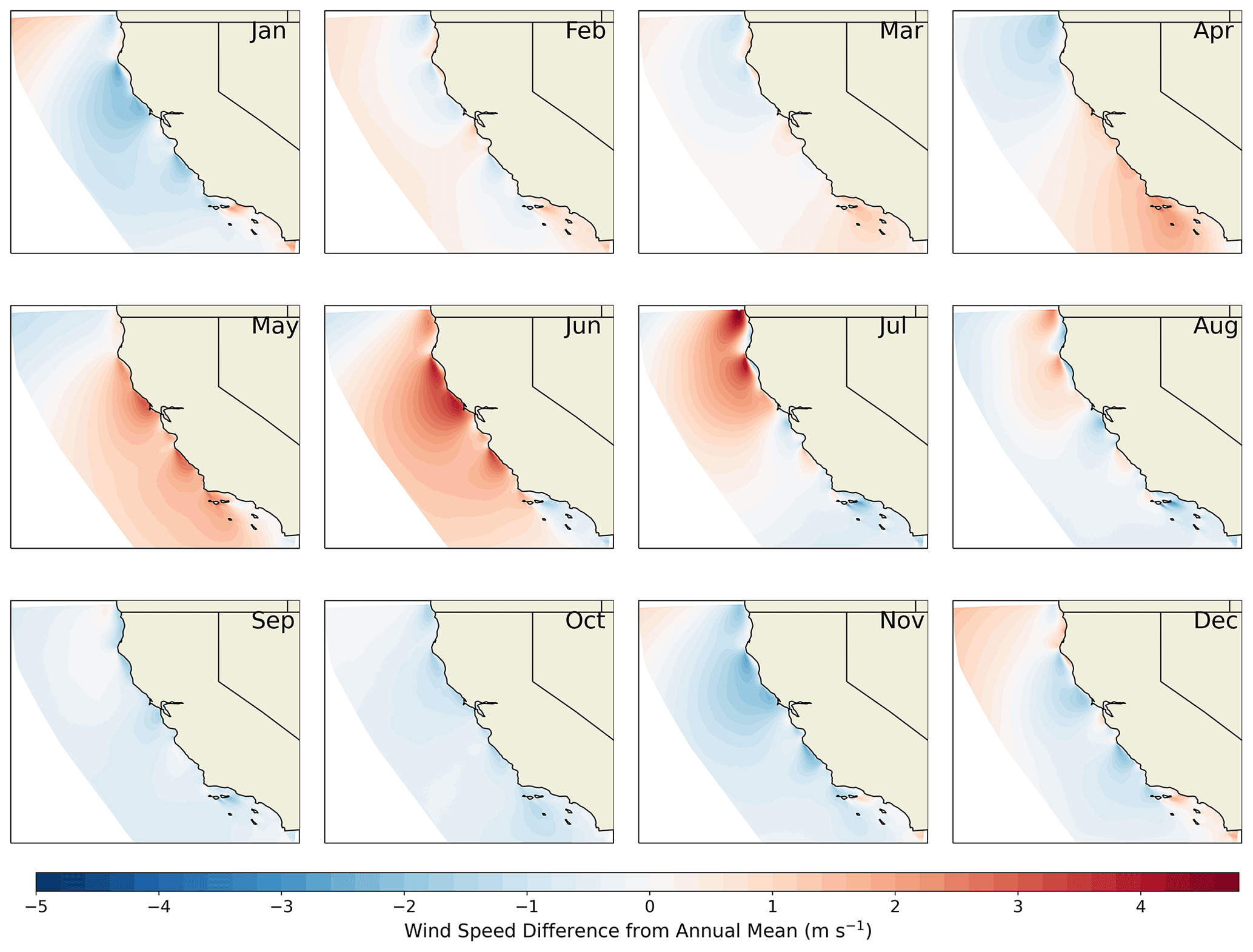
Figure A13 Maps showing the annual cycle in 160 m wind speed expressed in terms of the difference for each month's mean wind speed from the overall mean for the South Pacific region.

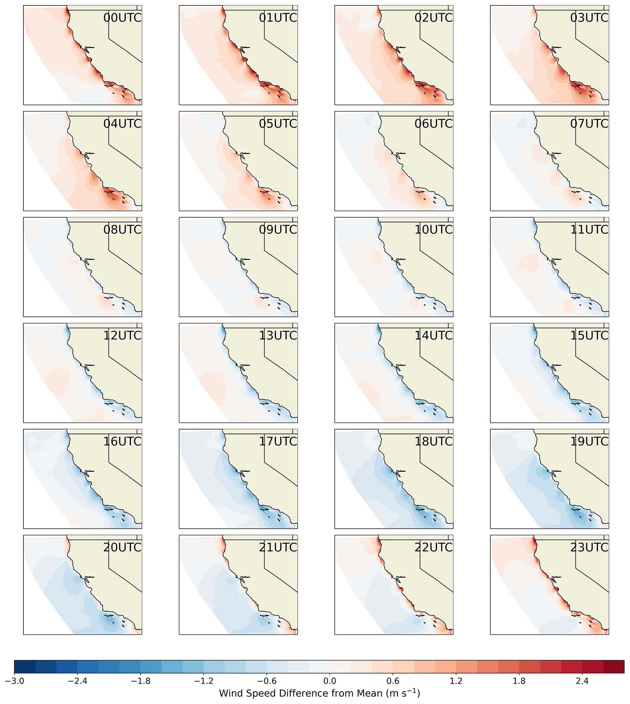
Figure A14 Maps showing the diurnal cycle in 160 m wind speed expressed in terms of the difference for each (UTC) hour's mean wind speed from the overall mean for the South Pacific region.

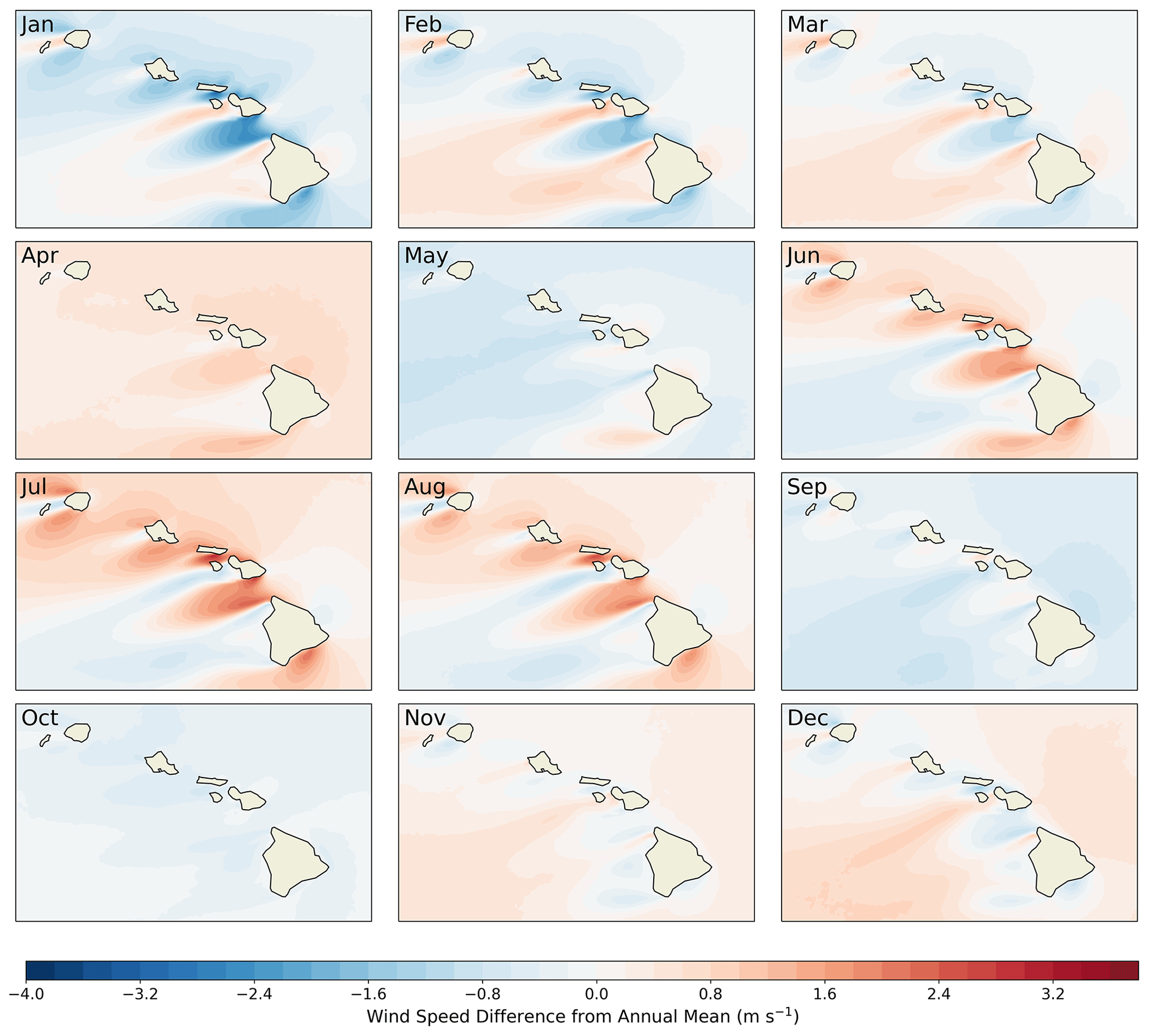
Figure A15 Maps showing the annual cycle in 160 m wind speed expressed in terms of the difference for each month's mean wind speed from the overall mean for the Hawaii region.

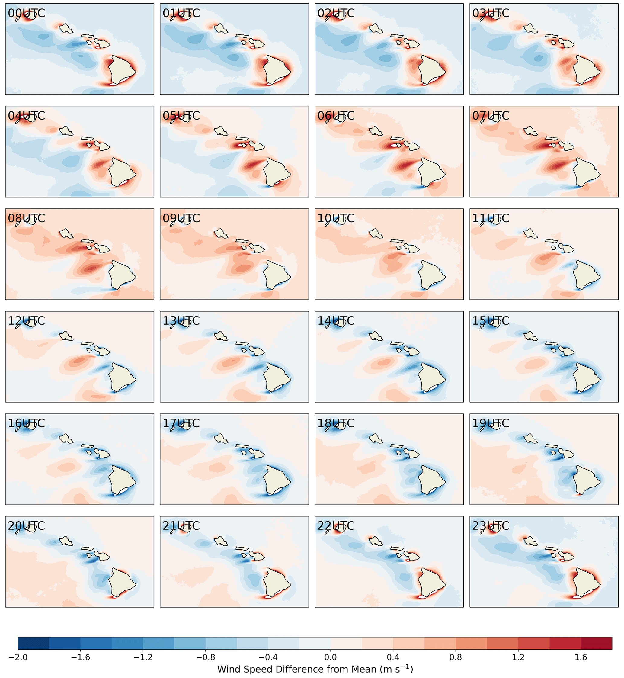
Figure A16 Maps showing the diurnal cycle in 160 m wind speed expressed in terms of the difference for each (UTC) hour's mean wind speed from the overall mean for the Hawaii region.

Appendix B: Wind speed differences between NOW-23 overlapping regional domain boundaries

When two NOW-23 WRF model domains are adjacent (North Atlantic and Mid-Atlantic, Mid-Atlantic and South Atlantic, South Atlantic and Gulf of Mexico, and North Pacific and South Pacific), there is some limited spatial overlap. In this section, we compare the mean 160 m wind speed from neighboring domains in these limited overlapping regions to quantify the deviation between regional data sets and provide guidance to NOW-23 stakeholders.

In most cases, we find minimal differences between the NOW-23 regional data sets when they overlap consistently well within the model uncertainty. The deviation between the overlapping area from the Mid-Atlantic and the North Atlantic regional data sets (Fig. B1), which both use the same WRF model setup (with the MYNN PBL scheme), is smaller than 0.2 m s⁻¹ in either direction. Similarly, we observe limited differences in the overlapping region between the South Atlantic and the Mid-Atlantic domains (Fig. B2), which employ different WRF model setups. Near the coast, the difference is smaller than 0.2 m s⁻¹ in either direction. The mean difference increases in the open ocean in areas not directly relevant for offshore wind energy purposes. Additionally, the South Atlantic data set slightly (<0.2 m s⁻¹) models stronger wind speed compared to the Gulf of Mexico domain (Fig. B3), with some larger differences near the south edge of Florida.

On the US West Coast, a major difference appears, with the North Pacific data set modeling significantly stronger wind speed compared to the South Pacific one (Fig. B4). This difference is mainly due to the fact that the two regional data sets adopt different PBL schemes which have been shown to produce significantly different results on the US West Coast, as detailed in the previous sections.

For these limited areas where the WRF model domains overlap, stakeholders can access NOW-23 data from both neighboring regions for download. For all cases where mean differences are limited, the data from either region can be used with confidence. Considering the overlap between the South Atlantic and Gulf of Mexico domains, it is reasonable to expect that the Gulf of Mexico regional data set provides the most accurate data in the overlapping area south of Florida, as it captures all the metocean dynamics in the rest of the Gulf. Similarly, the South Atlantic domain is expected to be more accurate in the small region north of Florida where its WRF model domain overlaps with the Gulf of Mexico. Cape Cod could also be considered a natural barrier influencing somewhat different metocean conditions to the north and south, suggesting that the North Atlantic data set may be better suited for the region north of the Cape, while the Mid-Atlantic domain could be preferred for the region south of the Cape. It is important to note, however, that we did not validate these scientific speculations by comparing the NOW-23 modeled data in the overlapping regions against observations, given the limited differences between the regional data sets. For the overlap between the North Pacific and South Pacific domains, we would like to remind users that only the South Pacific domain (and its WRF model configuration) underwent a regional tuning and validation, and therefore, that setup should be preferred for the region of overlap.

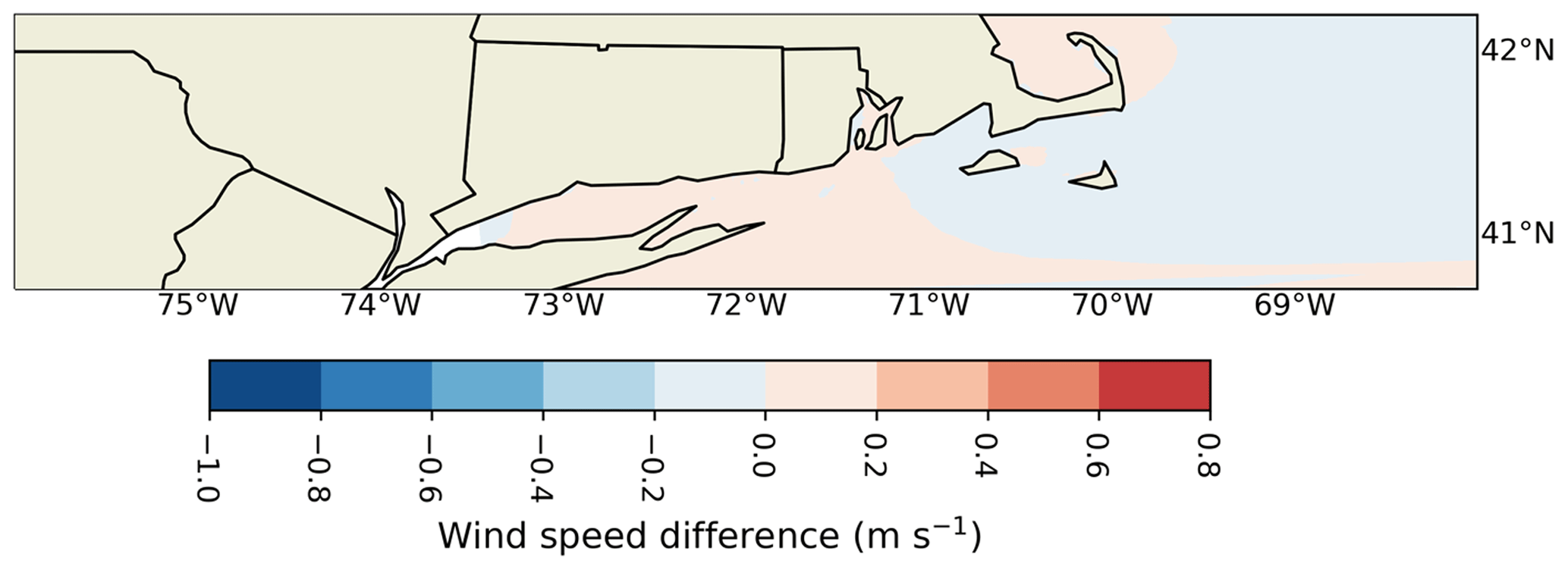
Figure B1 Map showing the difference in mean 160 m wind speed between the North Atlantic regional data set and the Mid-Atlantic one in the region where their WRF model domains overlap.

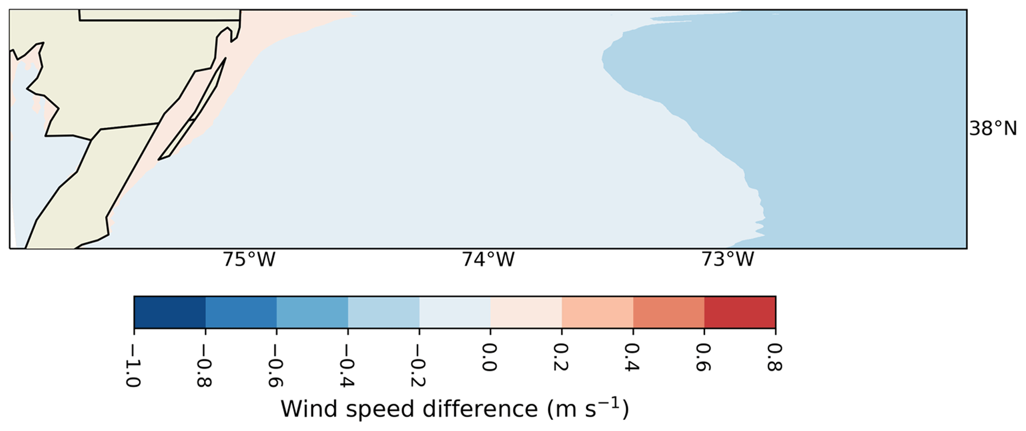
Figure B2 Map showing the difference in mean 160 m wind speed between the Mid-Atlantic regional data set and the South Atlantic one in the region where their WRF model domains overlap.

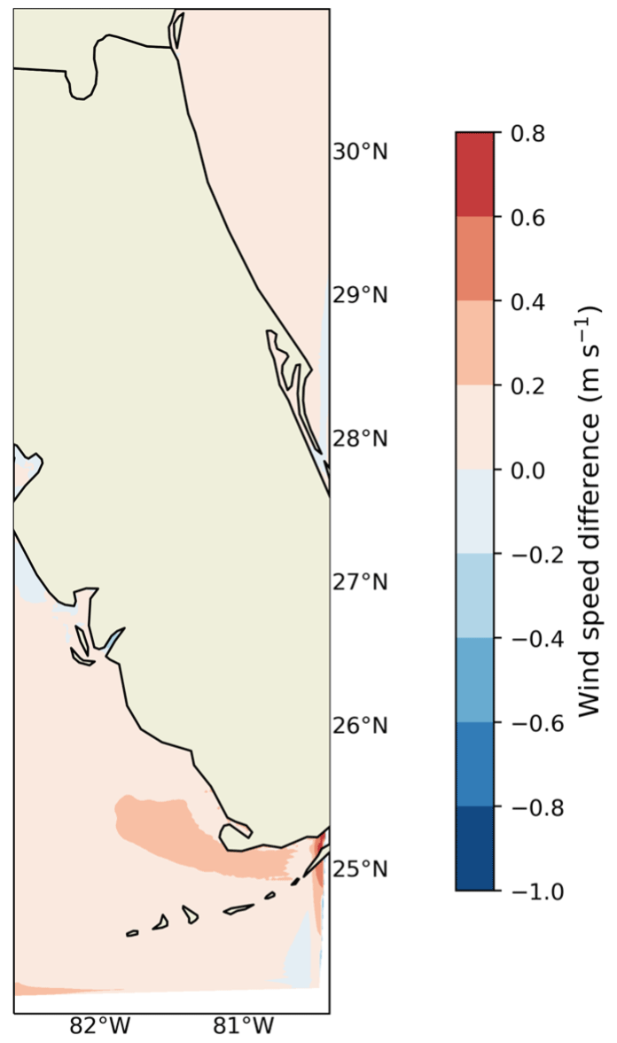
Figure B3 Map showing the difference in mean 160 m wind speed between the South Atlantic regional data set and the Gulf of Mexico one in the region where their WRF model domains overlap.

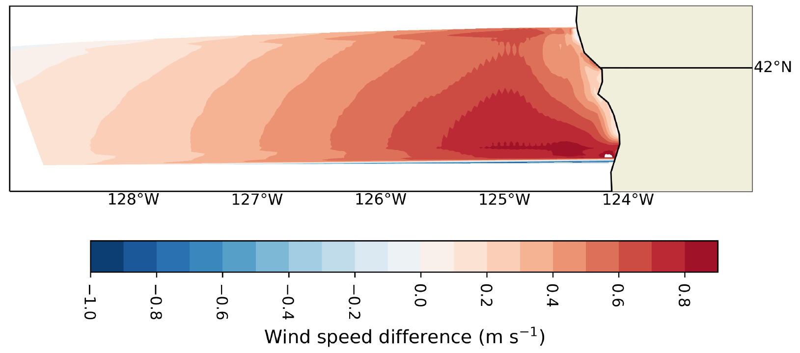
Figure B4 Map showing the difference in mean 160 m wind speed between the North Pacific regional data set and the South Pacific one in the region where their WRF model domains overlap.

Appendix C: Comparison between NOW-23 and the WIND Toolkit

Figure C1 presents a comparison of mean wind speeds between the NOW-23 data set and the 7-year (2007–2013) WIND Toolkit for the offshore regions in the contiguous United States. We note that Hawaii was not part of the WIND Toolkit domain, so a direct comparison between the NOW-23 data set and the WIND Toolkit for this region is not possible. NOW-23 and the WIND Toolkit have many differences (e.g., different length of the period of record, different reanalysis forcing, and different WRF model version). However, the magnitude of the differences in mean wind speed between the two data sets seems largely connected, in most regions, to the PBL schemes being adopted in the two data sets. The WIND Toolkit used the YSU PBL scheme across all regions, whereas, as described in this paper, NOW-23 uses either the MYNN or the YSU PBL scheme based on the results of a region-specific validation. For the Mid-Atlantic, North Atlantic, Great Lakes, and North Pacific regions, the NOW-23 data set (with the MYNN PBL scheme) consistently models stronger wind speeds compared to the WIND Toolkit, with differences larger than 0.5 m s⁻¹ in the Mid-Atlantic and North Pacific domains and even larger in the North Atlantic and Great Lakes regions. In the South Atlantic and Gulf of Mexico regions, the wind speeds between the NOW-23 data set (with the YSU PBL scheme) and the WIND Toolkit are similar across the majority of the domains. We note how, off the coast of Florida, the NOW-23 data set exhibits stronger hub height wind speeds, with differences larger than 0.5 m s⁻¹ compared to the WIND Toolkit. For the South Pacific region, despite both NOW-23 and the WIND Toolkit using the same PBL scheme (YSU), NOW-23 models stronger hub height winds off the coast of central and southern California, with some local differences on the order of 1 m s⁻¹.

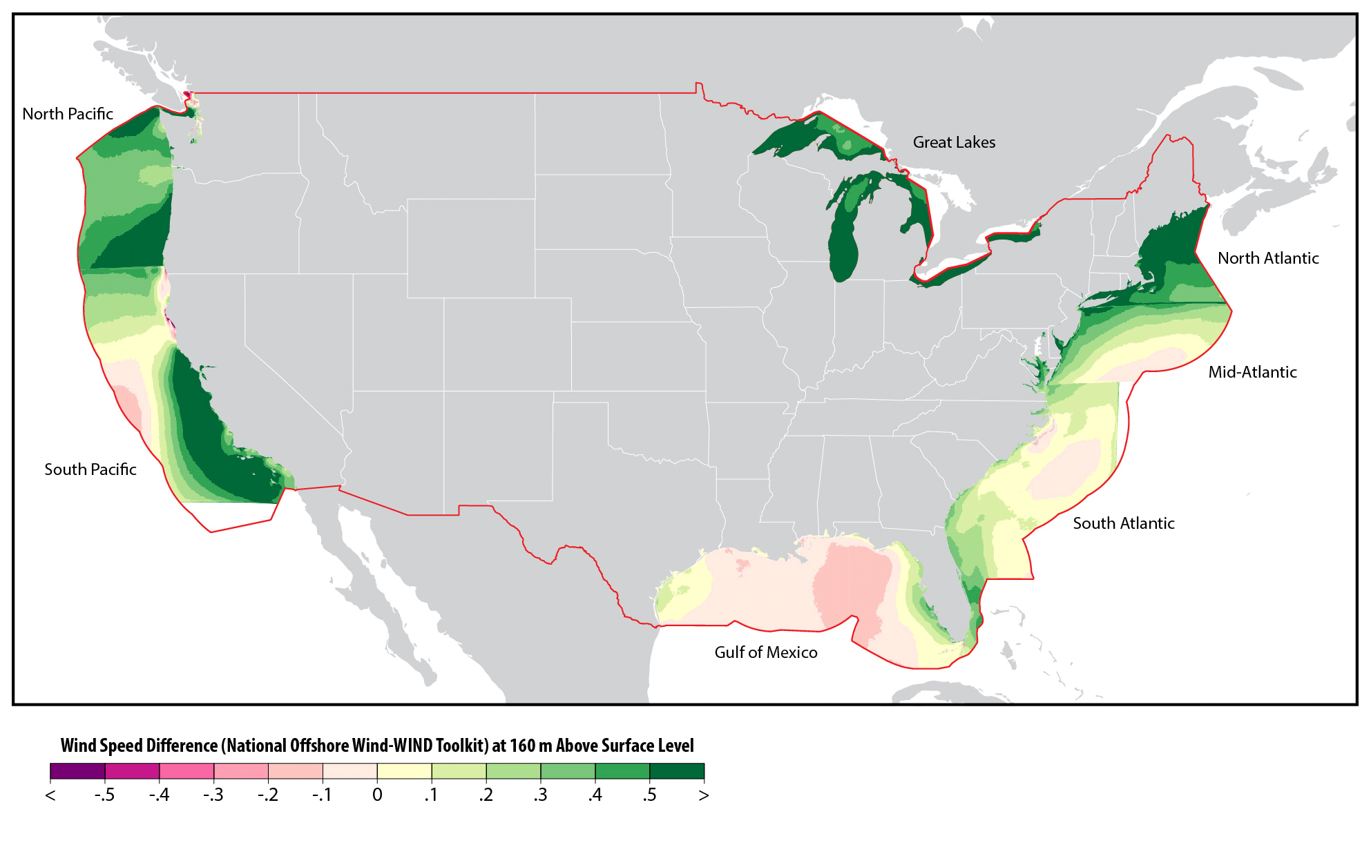
Figure C1 Map showing the difference in mean 160 m wind speed between the NOW-23 data set and the WIND Toolkit for the EEZ in the contiguous US where the two data sets overlap. The difference is calculated using the full temporal extent of each data set (2000–2019/2022 for NOW-23; 2007–2013 for the WIND Toolkit).