the Creative Commons Attribution 4.0 License.
the Creative Commons Attribution 4.0 License.
 | 16 Apr 2024
Synthesis Product for Ocean Time Series (SPOTS) – a ship-based biogeochemical pilot
Nico Lange
Björn Fiedler
Marta Álvarez
Alice Benoit-Cattin
Heather Benway
Pier Luigi Buttigieg
Laurent Coppola
Kim Currie
Susana Flecha
Dana S. Gerlach
Makio Honda
I. Emma Huertas
Siv K. Lauvset
Frank Muller-Karger
Arne Körtzinger
Kevin M. O'Brien
Sólveig R. Ólafsdóttir
Fernando C. Pacheco
Digna Rueda-Roa
Ingunn Skjelvan
Masahide Wakita
Angelicque White
The presented pilot for the Synthesis Product for Ocean Time Series (SPOTS) includes data from 12 fixed ship-based time-series programs. The related stations represent unique open-ocean and coastal marine environments within the Atlantic Ocean, Pacific Ocean, Mediterranean Sea, Nordic Seas, and Caribbean Sea. The focus of the pilot has been placed on biogeochemical essential ocean variables: dissolved oxygen, dissolved inorganic nutrients, inorganic carbon (pH, total alkalinity, dissolved inorganic carbon, and partial pressure of CO2), particulate matter, and dissolved organic carbon. The time series used include a variety of temporal resolutions (monthly, seasonal, or irregular), time ranges (10–36 years), and bottom depths (80–6000 m), with the oldest samples dating back to 1983 and the most recent one corresponding to 2021. Besides having been harmonized into the same format (semantics, ancillary data, units), the data were subjected to a qualitative assessment in which the applied methods were evaluated and categorized. The most recently applied methods of the time-series programs usually follow the recommendations outlined by the Bermuda Time Series Workshop report (Lorenzoni and Benway, 2013), which is used as the main reference for “method recommendations by prevalent initiatives in the field”. However, measurements of dissolved oxygen and pH, in particular, still show room for improvement. Additional data quality descriptors include precision and accuracy estimates, indicators for data variability, and offsets compared to a reference and widely recognized data product for the global ocean: the GLobal Ocean Data Analysis Project (GLODAP). Generally, these descriptors indicate a high level of continuity in measurement quality within time-series programs and a good consistency with the GLODAP data product, even though robust comparisons to the latter are limited. The data are available as (i) a merged comma-separated file that is compliant with the World Ocean Circulation Experiment (WOCE) exchange format and (ii) a format dependent on user queries via the Environmental Research Division's Data Access Program (ERDDAP) server of the Global Ocean Observing System (GOOS). The pilot increases the data utility, findability, accessibility, interoperability, and reusability following the FAIR philosophy, enhancing the readiness of biogeochemical time series. It facilitates a variety of applications that benefit from the collective value of biogeochemical time-series observations and forms the basis for a sustained time-series living data product, SPOTS, complementing relevant products for the global interior ocean carbon data (GLobal Ocean Data Analysis Project), global surface ocean carbon data (Surface Ocean CO2 Atlas; SOCAT), and global interior and surface methane and nitrous oxide data (MarinE MethanE and NiTrous Oxide product).
Aside from the actual data compilation, the pilot project produced suggestions for reporting metadata, implementing quality control measures, and making estimations about uncertainty. These recommendations aim to encourage the community to adopt more consistent and uniform practices for analysis and reporting and to update these practices regularly. The detailed recommendations, links to the original time-series programs, the original data, their documentation, and related efforts are available on the SPOTS website. This site also provides access to the data product (DOI: https://doi.org/10.26008/1912/bco-dmo.896862.2, Lange et al., 2024) and ancillary data.
- Article
(2063 KB) - Full-text XML
-
Supplement
(659 KB) - BibTeX
- EndNote


Continuing global anthropogenic carbon dioxide emissions in combination with increasing nutrient inputs into the ocean over the past decades have resulted in unprecedented changes in the ocean biogeochemistry (O'Brien et al., 2017; Friedlingstein et al., 2022) and marine ecosystem states (e.g., Edwards et al., 2013; Barton et al., 2016). As climate change progresses, these complex changes will be aggravated (Bopp et al., 2013; Cooley et al., 2022).
To disentangle natural variability, occurring on a range of temporal and spatial scales (Valdés and Lomas, 2017), and human-induced changes in marine ecosystems (Henson et al., 2016; Benway et al., 2019), decades of sustained fixed-location time-series observations are required. Following recommendations from international programs such as the Joint Global Ocean Flux Study (JGOFS, 1990) and Global Ocean Ecosystem Dynamics (GLOBEC, 1997), only a few ship-based fixed ocean time-series programs have been established around the globe since the late 1980s. The ongoing observations of these programs have captured the evolving changes in ocean biogeochemistry and the associated impacts on marine food webs, marine biodiversity, and ecosystems. Examples of observed changes include changes in the ocean's anthropogenic carbon inventory, oxygen levels, seawater pH, ventilation rates, and vertical nutrient transports (e.g., Bates et al., 2014; Tanhua et al., 2015; Neuer et al., 2017). Even though the collective value of multiple time-series data is greater than that provided by each individual time series, ship-based time-series programs have primarily been launched to support the specific goals of individual programs and ancillary projects. The International Group of Marine Ecological Time Series (IGMETS, O'Brien et al., 2017) demonstrated the collective value by performing an integrative and collective assessment of over 340 ship-based time series, thereby increasing the range of spatial and temporal scales that can be addressed and highlighting the importance of joint and multidisciplinary time-series observation programs (Valdés and Lomas, 2017).
Despite their indisputable importance and the wealth of ship-based time-series data, difficulties in data discoverability, accessibility, and interoperability presently limit ship-based time-series data utilization, the realization of their full scientific potential, and the overall recognition of the programs (Benway et al., 2019; Tanhua et al., 2019). Moreover, these challenges have prevented shipboard time series from becoming a more formalized and endorsed component of the Global Ocean Observing System (GOOS, Moltmann et al., 2019). In addition to the lack of a community-agreed time-series data public-release agreement, which leads to free sharing of time-series data being uncommon, the lack of standardized formats, semantics, units, scales, standards, quality assurance and control, metadata reporting, and user interfaces across and within time-series sites represents the main data challenge. The usage of different measurement protocols, sometimes without comprehensive reporting of the corresponding variable-inherent uncertainties, and the time-consuming manual data retrieval at multiple access points are further prone to data-handling errors. Existing biogeochemical (BGC) data synthesis products have already tackled these challenges for other observation types and have increased the utility of large amounts of individual datasets, e.g., the MarinE MethanE and NiTrous Oxide product (MEMENTO, Kock and Bange, 2015), the Global Ocean Data Analysis Project (GLODAP, Lauvset et al., 2022) and the Surface Ocean CO2 Atlas (SOCAT, Bakker et al., 2016a). However, neither IGMETS (O'Brien et al., 2017) nor OceanSites (Weller et al., 2016), a global network of long-term autonomous open-ocean reference stations, has generated a global data synthesis product of time-series data that would complement existing BGC data synthesis products.
To address these shortcomings and to follow up on the Bermuda Time Series workshop from 2013 (Lorenzoni et al., 2013), both the Ocean Carbon and Biogeochemistry program and the EU Horizon 2020 project EuroSea convened in workshops with several time-series operators. Resulting from these workshops, a call was formulated for a pilot data synthesis product of well-established time-series programs that focuses on a limited set of variables. Further, a roadmap was created to develop a pilot product that aims to establish a findable, accessible, interoperable, and reusable (FAIR, Wilkinson et al., 2016) data management plan for shipboard ocean time series (Benway et al., 2020). This goes hand in hand with the GOOS Implementation Roadmap (GOOS, 2020), calling for more systematic and sustainable approaches for climate-relevant observations across ocean data platforms and networks (Belward et al., 2016), especially regarding the GOOS-defined scientific applications: the ocean carbon content (Q1.1), ocean dead zones (Q2.1), rates of acidification (Q2.2), and ocean productivity (Q3.2).
Following these calls, here, we describe the resultant Synthesis Product for Ocean Time Series (SPOTS) pilot, synthesizing high-quality data from 12 global ship-based time-series sites with a focus on BGC essential ocean variables (EOVs). This paper briefly presents the included time-series programs (Sect. 2), describes the methods applied to compile and assess the product (Sect. 3) and to conduct data quality assessment (Sect. 4), describes the final product (Sect. 5), elaborates on the stakeholder usability (Sect. 6), and describes the data access (Sect. 7). Finally, the main findings of the effort are presented (Sect. 8), and next steps to guarantee the continuity and success of SPOTS are identified (Sect. 9).
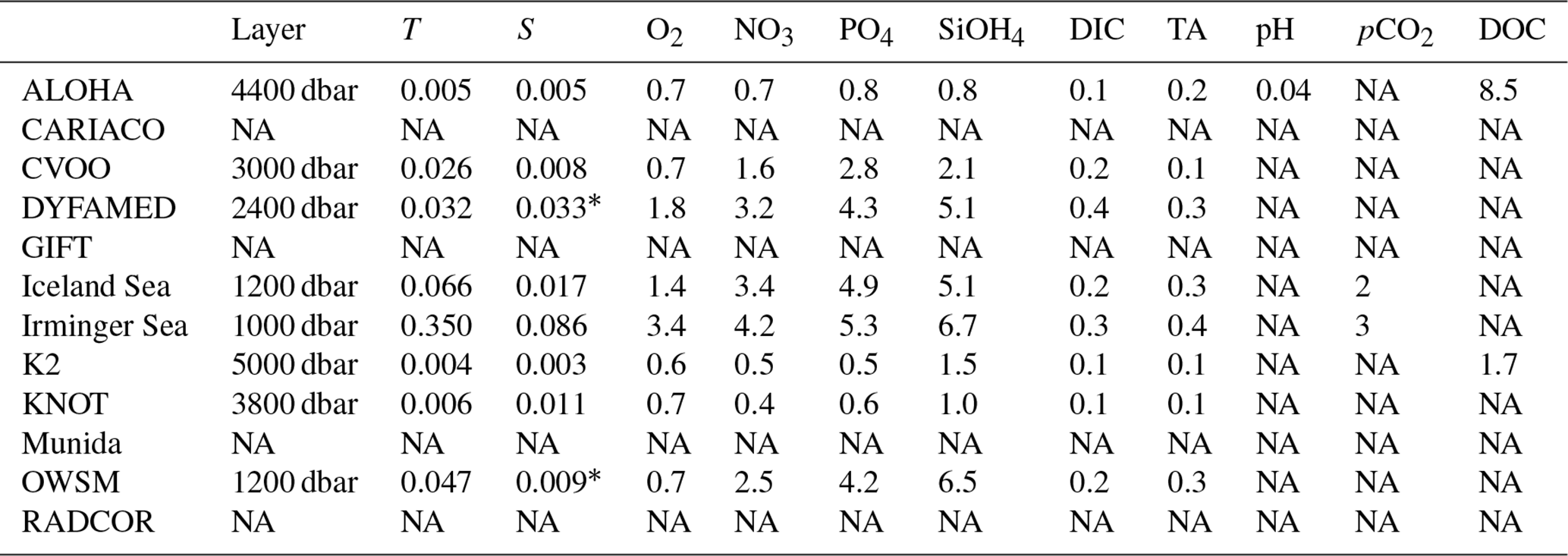
The SPOTS pilot includes data from 12 fixed ship-based time-series programs (Fig. 1), all of which routinely measure BGC EOVs. All major climate zones are covered, although not all ocean biogeochemical zones are (Reygondeau et al., 2013). Existing datasets were extended whenever possible by publicly available and more recent data (Table S1 in the Supplement). In addition to capturing different marine environments (Sect. 2.1), the characteristics of the time-series programs also differ in terms of the station visit frequency, i.e., the temporal resolution (monthly, seasonal, or irregular); the time range of the observational period; the bottom depth; and whether a dedicated research vessel is used (Table 1). If a time-series program consists of two or more related stations, usually the deepest station was selected. The included data from the Gibraltar Fixed Time series (GIFT) and the RADIALES A Coruña (RADCOR) program display exceptions to this rule as, for both sites, data from three related stations were selected.
Table 1Key metadata of participating time-series programs. Ordered according to ocean basin: Pacific (4), Atlantic (3), marginal seas (2), Nordic Seas (3). T refers to temperature (CTD), S refers to salinity (either bottle or CTD data; the asterisk denotes if more than 50 % of station visits are CTD data only), O2 refers to oxygen, NO3 refers to dissolved nitrate, NO2 refers to dissolved nitrite, PO4 refers to dissolved phosphate, SiOH4 refers to dissolved silicate, NH4 refers to dissolved ammonium, DIC refers to dissolved inorganic carbon, TA refers to total alkalinity, pCO2 refers to partial pressure of carbon dioxide, POC refers to particulate organic carbon, PON refers to particulate organic nitrogen, POP refers to particulate organic phosphorus, TPC refers to total particulate carbon, TPN refers to total particulate nitrogen, TPP refers to total particulate phosphorus, DOC refers to dissolved organic carbon, and NA denotes not available.
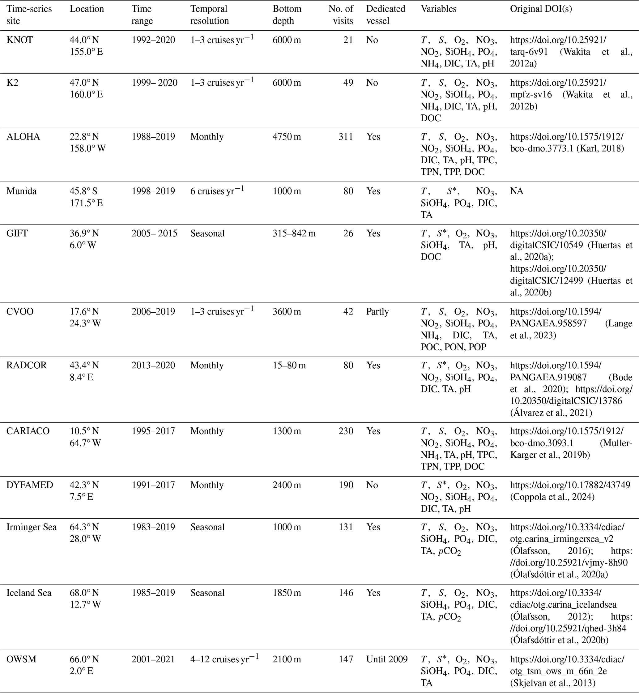
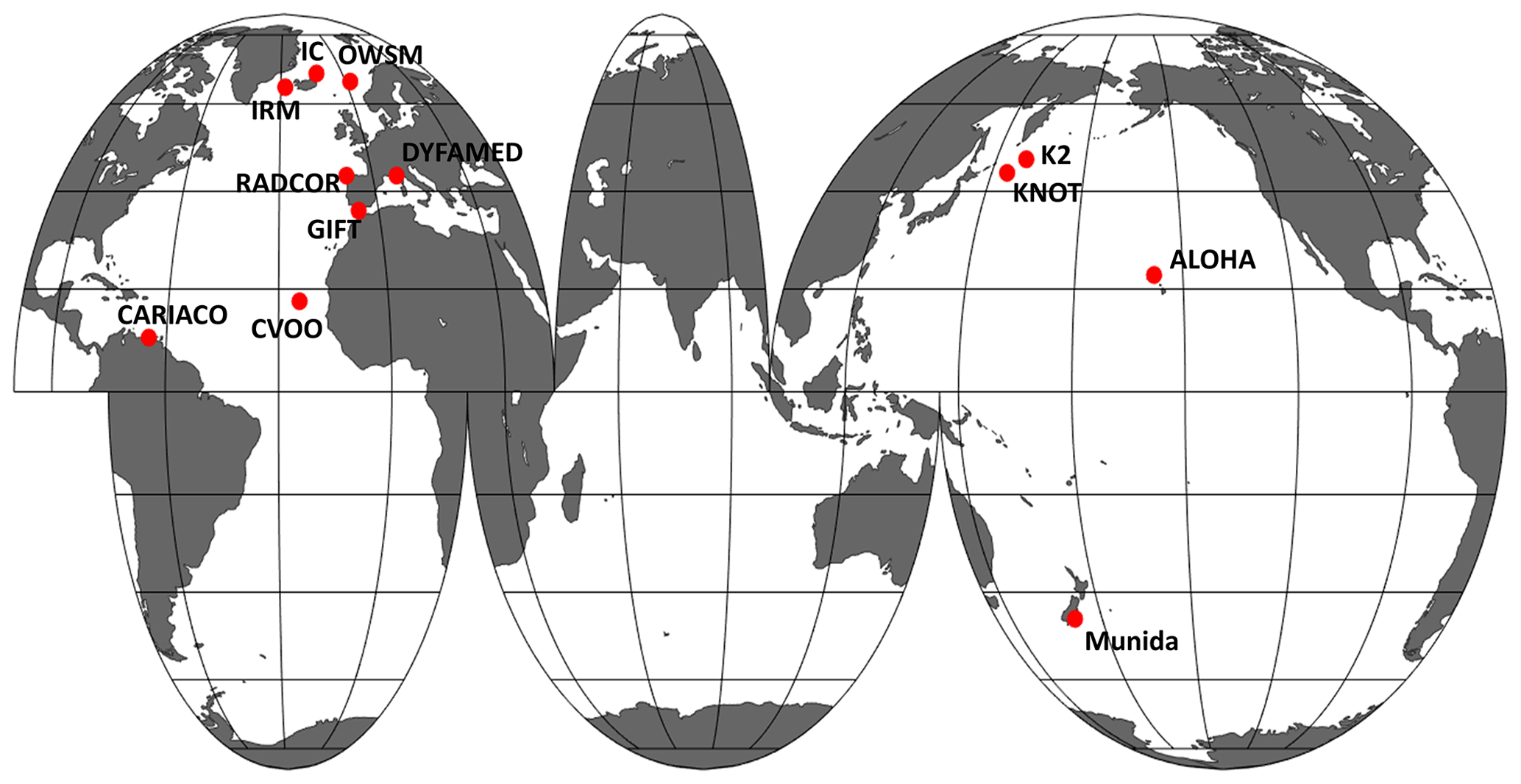
Figure 1Locations of participating ship-based time-series stations.
2.1 Marine environment of time series sites
2.1.1 A Long-term Oligotrophic Habitat Assessment (ALOHA)
The deep-water (∼ 4750 m) time-series station of the Hawaii Ocean Time Series program (HOT), ALOHA (A Long-term Oligotrophic Habitat Assessment; Karl and Church, 2019), is located 100 km north of Oahu, Hawaii, more than 1 Rossby radius (50 km) away from the steep topography associated with the Hawaiian Ridge. ALOHA serves as an open-ocean benchmark, and its research goals are aligned with the main objectives of the JGOFS and the World Ocean Circulation Experiment (WOCE). One of the principles of the HOT program is to observe seasonal and interannual variations in water mass characteristics and BGC variables. The monthly measurements since 1988 are representative of the oligotrophic North Pacific eastern subtropical gyre, with station ALOHA lying in the center of the North Pacific and North Equatorial Current. Typically, the site is characterized by a relatively deep permanent pycnocline (and nutricline) and a shallow mixed-layer depth. Intermittent local wind forcing caused by extratropical cyclones' cold fronts impacts the annual cycle of the surface waters (Karl et al., 1996).
2.1.2 CArbon Retention In A Colored Ocean (CARIACO)
The station of the CARIACO (CArbon Retention In A Colored Ocean) oceanographic time series program (Muller-Karger et al., 2019a) is located in the Cariaco Basin, a semi-enclosed tectonic depression located on the continental shelf off northern Venezuela in the southern Caribbean Sea. The Cariaco Basin is composed of two sub-basins approximately 1400 m in depth that are connected to the Caribbean Sea by two shallow (140 m deep) channels. These channels allow for the open exchange of near-surface water. The restricted circulation below the 140 m sills, coupled with highly productive surface waters due to seasonal wind-driven coastal upwelling (around 450 g C m−2 yr−1; Muller-Karger et al., 2010), has led to sustained anoxia below around 250 m. The goal of the near-monthly measurements at CARIACO between 1995 and 2017 was to observe linkages between oceanographic processes and the production, remineralization, and sinking flux of particulate matter in the Cariaco Basin and how these change over time. It also aimed to understand climatic changes in the region.
2.1.3 Cape Verde Ocean Observatory (CVOO)
The Cape Verde Ocean Observatory (CVOO) is located in the eastern tropical North Atlantic, about 800 km from the west coast of Africa, which is influenced by the seasonal eastern boundary upwelling system, high Saharan dust deposition rates, and frequently passing eddies (Schütte et al., 2016). It is part of the Cape Verde Observatory, which also includes an operational atmospheric monitoring site. The combined observations aim to investigate long-term changes in greenhouse gas concentrations in the atmosphere and in the ocean in a key region for air–sea interactions. The irregular measurements of BGC variables at CVOO started in 2006 and are still ongoing, and the project is striving toward more regular measurements in the future by having a dedicated vessel available. The station has a bottom depth of 3600 m and lies in the center of the Cape Verde Fontal Zone, resulting in large variations in the present oligotrophic water masses. The frontal zone separates most of the eastern tropical North Atlantic from the anticyclonic subtropical gyre system in the North Atlantic (Stramma et al., 2005). This further results in an ocean shadow zone and an oxygen-poor layer between 400 to 500 m (Stramma et al., 2008), which is being sampled at CVOO. Below the mixed layer, subtropical underwater from the subtropical gyre system, as well as North Atlantic Central Water and South Atlantic Central Water, can be present (Tomczak, 1981; Pastor et al., 2008).
2.1.4 DYFAMED
DYFAMED (DYnamique des Flux Atmosphériques en MEDiterranée et leur évolution dans la colonne d'eau; i.e., DYnamics of Atmospheric Fluxes in the Mediterranean Sea) is located in the central part of the Ligurian Sea, about 50 km off Nice, on the Nice Corsica transect, and is representative of open-sea western Mediterranean basin waters. Ongoing multidisciplinary monthly measurements at DYFAMED have been performed since 1991, observing the following: (i) the evolution of the water mass properties, (ii) the carbon export change, and (iii) the variability in the biological species relative to climate forcing. The water column can be divided into three principal layers: deep, intermediate, and surface. The latter, typically for the Mediterranean trophic environment, experiences large seasonal variability. Further, the Northern Current front acts as a barrier to exchanges with the coastal zone of the Ligurian Sea and prevents DYFAMED from experiencing lateral inputs (Vescovali et al., 1998). Consequently, the primary production depends on inputs of nutrients from deeper waters and atmospheric inputs of nitrogen and some trace metals, particularly during summer (Miquel, 2011). The DYFAMED site is characterized by intermediate water (300–400 m) that is lower in oxygen concentrations (Levantine Intermediate Water) and deep water that is richer in oxygen, primarily induced by vertical mixing occurring in winter during intense and cold winds (convection processes; Coppola et al., 2018).
2.1.5 Gibraltar Fixed Time series (GIFT)
Seasonal measurements at the GIFT sites were established in 2005 to quantify the exchange of carbon between the Mediterranean Sea and the adjacent Atlantic Ocean and to assess the temporal evolution of BGC fluxes. The three GIFT time-series stations (Flecha et al., 2019) are located along the longitudinal axis of the Strait of Gibraltar, which connects the two basins. The Strait is surrounded by the Gulf of Cádiz (west) and the Alboran Sea (east). Water circulation in the channel can be described as a bi-layer system characterized by an inward (eastward) flow of the North Atlantic Central Water in the upper layer and an outward (westward) flow of Mediterranean waters (predominantly formed by a mixture of the Levantine Intermediate Water and the Western Mediterranean Deep Water) at the bottom layer. The depth and thickness of each water mass vary along the Strait due to topography in the channel and the influence of physical mechanisms. In particular, the Espartel sill (358 m depth) and the Camarinal sill (285 m depth) lead to large variability in the proportion of the water flows' position. Therefore, sampling depths vary from one campaign to another due to the instant position of the incoming and outcoming flows that are identified by their thermohaline properties through the conductivity–temperature–depth (CTD) casts.
2.1.6 Irminger Sea station (IRM-TS) and Iceland Sea station (IC-TS)
In 1983, seasonal measurements at the IRM-TS and the IC-TS (Olafsson et al., 2010) were initiated to observe the seasonal variability in carbon–nutrient chemistry in the North Atlantic off the Iceland shelf. The stations are located in two hydrographically different regions to the north and southwest of Iceland (Takahashi et al., 1985; Peng et al., 1987). The station in the northern Irminger Sea (IRM-TS) is characterized by relatively warm and saline (S>35) Modified North Atlantic Water derived from the North Atlantic Drift. Winter mixing is induced by strong winds and loss of heat to the atmosphere. This location may also be described as representing the subpolar gyre (Hatún et al., 2005). The IC-TS is located in the central Iceland Sea north of the Greenland–Scotland Ridge. At the IC-TS, cold Arctic Intermediate Water, formed from Atlantic Water and low-salinity Polar Water, usually predominates and overlays Arctic Deep Water (Olafsson et al., 2009). The Polar Water influence in the surface layers is variable (Stefansson, 1962; Hansen and Østerhus, 2000). Both regions are important sources of North Atlantic Deep Water.
2.1.7 K2 and KNOT
The K2 and KNOT stations (Wakita et al., 2017) are located approximately 400 km northeast of Hokkaido Island, Japan, in the subarctic western North Pacific. Since 1999 and 1992, respectively, irregular field observations have been conducted at these stations to investigate the inorganic carbon system dynamics in response to variations in hydrography and biological processes. The overarching goal is to investigate the response of the biological pump to climate forcing in the western subarctic Pacific gyre. The region is characterized by high primary productivity and abundant marine resources (FAO, 2016) and might be the first region of the ocean to become undersaturated with respect to calcium carbonate during winter (Orr et al., 2005). The sites are representative of the southwestern subarctic gyre, with both stations lying offshore of the Oyashio Current and just north of the subpolar front. Seasonal cycles are present (e.g., Takahashi et al., 2006; Tsurushima et al., 2002; Wakita et al., 2013), with a highly productive biological pump from spring to fall and strong vertical mixing of deep waters that are rich in dissolved inorganic carbon (DIC) in winter.
2.1.8 Munida
This deep-water station is located in the Southwest Pacific Ocean, 65 km off the southeast coast of New Zealand, and is part the Munida Time Series Transect, which is sampled every 2 months. Measurements at Munida were established in 1998 to study the role of these waters in the uptake of atmospheric carbon dioxide and the seasonal, interannual, and long-term changes in the carbonate chemistry. The subantarctic waters are a sink for atmospheric carbon dioxide (Currie et al., 2011), and the seasonal cycles of DIC are primarily driven by net community production (Brix et al., 2013; Jones et al., 2013), with modification by the annual cycle of sea surface temperature.
2.1.9 Ocean Weather Station Mike (OWSM)
Ocean Weather Station Mike (OWSM) is located in the Norwegian Sea at the western baroclinic branch of the northward-flowing Norwegian Atlantic Current, where the water depth is 2100 m (Skjelvan et al., 2008, 2022). Hydrographic measurements date back to 1948, while carbonate chemistry measurements started in 2001 to monitor long-term changes in the biogeochemistry. Between 2001 and 2009, the station was sampled monthly, and since 2010, the sampling frequency has been four to six times per year. The site encompasses the cold Norwegian Sea Deep Water and the Arctic Intermediate Water in addition to the relatively warm and saline Atlantic Water. Occasionally, during late summer, fresh Norwegian Coastal Current Water meanders all the way out to OWSM, influencing the surface water at the station. Seasonal variability is observed in the uppermost ∼ 200 m, and long-term trends of carbonate variables are observed at all water depths. Over time, the surface water CO2 content at OWSM has increased at a faster rate than atmospheric pCO2 at this site (Skjelvan et al., 2022).
2.1.10 RADIALES A Coruña (RADCOR)
The RADIALES program started in 1989, aiming to obtain reliable baselines for long-term studies on climate change and ecosystem dynamics in times of increasing anthropogenic disturbances along the northern and northwestern Spanish coasts (Valdés et al., 2021). The program consists of monthly multidisciplinary perpendicular sections covering the Cantabrian Sea and the northwest coastal and neritic Spanish ocean. The A Coruña (NW Galician coast) section (RADIALES A Coruña, RADCOR) started in 1990 (Bode et al., 2020), and CO2 variables have been incorporated since 2013 in two stations, E2CO and E4CO. RADCOR is located on the northern edge of the Iberian Upwelling Region. Here, the classical pattern of seasonal stratification of the water column in temperate regions is masked by upwelling events from May to September. These upwelling events provide nutrients to support both primary and secondary production in summer. Nevertheless, upwelling is highly variable in intensity and frequency, demonstrating substantial interannual variability, mostly affecting the E2CO station (80 m), while the station closest to the shore, E4CO (15 m), is more impacted by estuarine and benthic processes. The CO2 chemistry and ancillary data were partially published in Guallart et al. (2022) to assess the reliability of directly measuring, with a spectrophotometric method, seawater ion carbonate in time series.
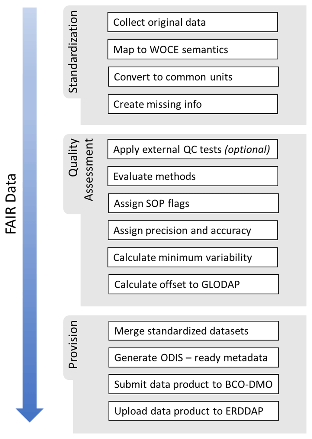
The data flow of the SPOTS pilot, depicting the main steps of the synthesis, is schematically illustrated in Fig. 2. In the following, the individual components of this data flow are described in detail.
3.1 Data collection
The data from the 12 participating time-series programs were retrieved from (multiple) data centers or were directly obtained from the responsible principal investigator (or using a combination of both) (Table S1 in the Supplement). In the latter case, merging, formatting, additional quality controlling (QC), and archiving of existing data were carried out. Only bottle data for BGC EOVs that had been measured by at least two of the participating programs were included in the pilot project, along with accompanying ancillary pressure, salinity, and temperature data. We have also developed a metadata template for BGC EOV ship-based time-series data (Table S2). The template has subsequently been used to collect all relevant metadata information from each participating time-series program. The collected metadata include general information about the program, such as information about the principal investigator and the location and timeframe of related station(s). The metadata also include detailed information on the measured variables – e.g., units; sampling and analytical methods and associated instrumentation; calculation, calibration, and quality control procedures; and standards or (certified) reference materials used. The latter not only vary among the time-series programs but can also vary within a time-series program over time.
3.2 Data assembly
The SPOTS pilot was created by standardizing data format, units, header names, primary QC flags, times, locations, and filling values and subsequently merging the individual datasets of each time-series program into one file. Only data that received a WOCE quality flag 2 (Table S3) were included in the product. Existing data were altered as little as possible without interpolation or calculation of “missing” variables. Similarly, original station, cast, and bottle numbers were kept or created artificially if non-existent to ensure consistency. The headers, units, and flags of the individual time-series datasets were standardized (Table S4) to conform with the WOCE exchange bottle data format (Swift and Diggs, 2008), a comma-delimited ASCII format for bottle data from hydrographic cruises. To enable an automated mapping to other existing vocabularies, we also mapped the WOCE headers to the Natural Environment Research Council (NERC) British Oceanographic Data Centre P01 vocabulary collection, as well as to the newly proposed BGC bottle standard by Jiang et al. (2022). We did not use the latter as “central” semantics due to the restrictions of existing QC tools, e.g., AtlantOS QC (Velo et al., 2021) and the crossover toolbox (Tanhua et al., 2010; Lauvset and Tanhua, 2015), in relation to WOCE semantics.
The standardization process also entailed unit conversions, most frequently from micromoles per liter (µmol L−1; nutrients and dissolved organic carbon (DOC)) or from micrograms per kilogram (µg kg−1; particulate matter) to micromoles per kilogram of seawater (µmol kg−1). The default procedure to convert from volumetric to gravimetric units was to use seawater density at an in situ salinity, reported laboratory temperature (otherwise assuming 20 °C as laboratory conditions), and pressure of 1 atm (following recommendations from Jiang et al., 2022). For some time-series datasets, the combined concentration of nitrate and nitrite was reported (Table S4). If explicit nitrite concentrations were provided, these were subtracted to obtain the nitrate values. If not, the combined concentration was renamed to nitrate assuming that the relative nitrite amount is negligible. For the HOT program specifically, low-level, high-sensitivity measurements of macronutrients (phosphate and nitrate) were available but not included in the pilot product. For total particulate carbon and total particulate nitrogen, the factors and (inverse standard atomic masses) were used, respectively, for the unit conversion to micromoles per kilogram. If neither temperature nor pressure was provided, all corresponding data entries were excluded from the product. The potential density anomaly1 is the only calculated variable. Missing and excluded values were set to −999.
3.3 Qualitative assessment of data
3.3.1 Internally applied quality control (QC)
The majority of the programs have established their own routines for QC and correspondingly flag their data using different flagging schemes. We did not double-check the applied flags, and we did not run additional QC checks. The applied QC for the collected stations includes statistical outlier checks of routinely measured pressure intervals using either a seasonal two- or three-sigma criterion , visual inspections of property–property plots (PPP), and application of crossovers using reference layers (Table S5). For example, K2 and KNOT used North Pacific Deep Water (NPDW), defined as the water mass between 27.69σθ (around 2000 dbar) and 27.77σθ (around 3500 dbar) (Wakita et al., 2017), as the reference layer for their internal crossover checks. For CVOO and Munida, we performed QC by applying a seasonal two-sigma criterion to the data, and for CVOO, we made additional use of comparisons to CANYON-B (Bittig et al., 2018) and crossovers. Since the QC procedures differ from program to program, we have provided recommendations for the QC of future data so that the flags are applied more consistently across different programs (Sect. 6.3). Further, the standardization of the SPOTS pilot also entailed mapping to a central flagging scheme. We chose the WOCE bottle flag scheme (Table S3). Flags indicating replicate measurements (WOCE flag of 6) were set to 2, whereas all other flags were set to 9, and the corresponding values were set to −999.
3.3.2 Method assessment
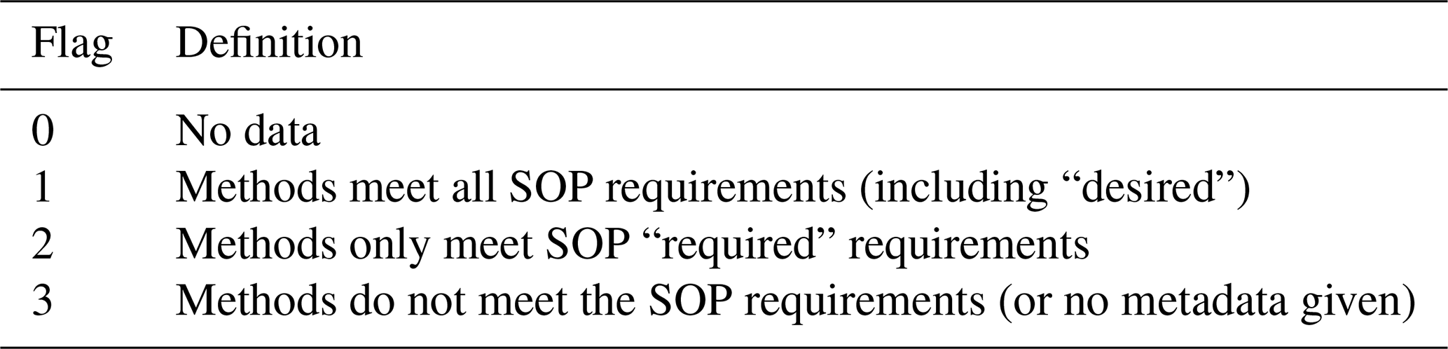
Given the inconsistencies in the applied internal quality checks and the fact that bias corrections following crossover analyses are presently impossible to apply to all included time-series datasets2, the comparability of the data for the SPOTS pilot was qualitatively assessed. The information on the applied methods of each time-series program, as provided through the metadata collection, was evaluated against methods recommended by prevalent initiatives in the field, i.e., known standard operating procedures (SOPs). SOP flags were assigned accordingly to each cruise of a time-series program (Table 2).
The majority of the defined SOP requirements used for the evaluation are based on the Bermuda Time Series Workshop report (Lorenzoni and Benway, 2013), with additional implementation of the following: GO-SHIP manuals (Langdon et al., 2010; Becker et al., 2019); the CARIACO Methods Manual (Astor et al., 2013); HOT analytical methods (https://hahana.soest.hawaii.edu/hot/protocols/protocols.html, last access: 3 April 2024), which are based on the Joint Global Ocean Flux Study protocols (IOC, 1994); the guide to BPs for ocean CO2 measurements (Dickson et al., 2007); results from the Scientific Committee on Research Working Group 147 “Towards comparability of global oceanic nutrient data” (Bakker et al., 2016b, c; Aoyama et al., 2010); and studies on preservation techniques for nutrients (e.g. Dore et al., 1996). The requirements were grouped into “required” and “desired” SOPs; see Table 3. To fulfill all requirements, i.e., to receive a SOP flag of 1, the metadata must show that the methods also met the corresponding desired requirements. Only time-series programs that provided granular metadata, i.e., metadata differentiating between different methods applied in time, could obtain a SOP flag of 1.
Using the example of total alkalinity (TA), we briefly explain the assessment method and related recommendations. For TA, two different methodologies meet our defined required recommendations: (i) potentiometric titration (Dickson et al., 2007), a procedure in which a seawater sample is placed in a cell (open or closed) where it is titrated with a solution of hydrochloric acid, following which TA is computed from the titrant volume and electromotive force (EMF) measurements (non-linear least-squares approach or a modified Gran approach), and (ii) the more recently emerging method where a spectrophotometric system is used to estimate TA by measuring the difference in absorbance at three wavelengths before injecting an acid with indicator solution to the seawater sample and after its injection (Yao and Byrne, 1998). If the TA data from a particular cruise of a time-series station were not estimated by either one of these two methods (or no metadata exist), a SOP flag 3 is assigned. The additional desired recommendations related to potentiometric titrations are that the potentiometric measurements were either executed using an open-cell titration (two-stage titration: total dissolved inorganic carbon is approximately zero in the pH region of 3.0 to 3.5 following SOP3b from Dickson et al., 2007) or that the corresponding curve-fitting method was documented (e.g., non-linear least-squares approach). Ideally, both of these recommendations are met, but for the pilot, and considering historical data with little metadata, meeting one of these desired recommendations was sufficient. For spectrophotometric measurements, the desired recommendation is that the indicator dye must be documented (e.g., bromocresol green). In addition, for both method types, the desired recommendations entail that measurements must have been calibrated using certified reference materials, and, if the samples were stored, the samples must have been poisoned and kept in a dark and cool location. If the TA data from a particular cruise of a time-series stations also meet these desired recommendations, a SOP flag 1 is assigned, otherwise a SOP flag 2 is given.
Table 3Recommendations by prevalent initiatives in the field with regard to the requirements for the method evaluation.
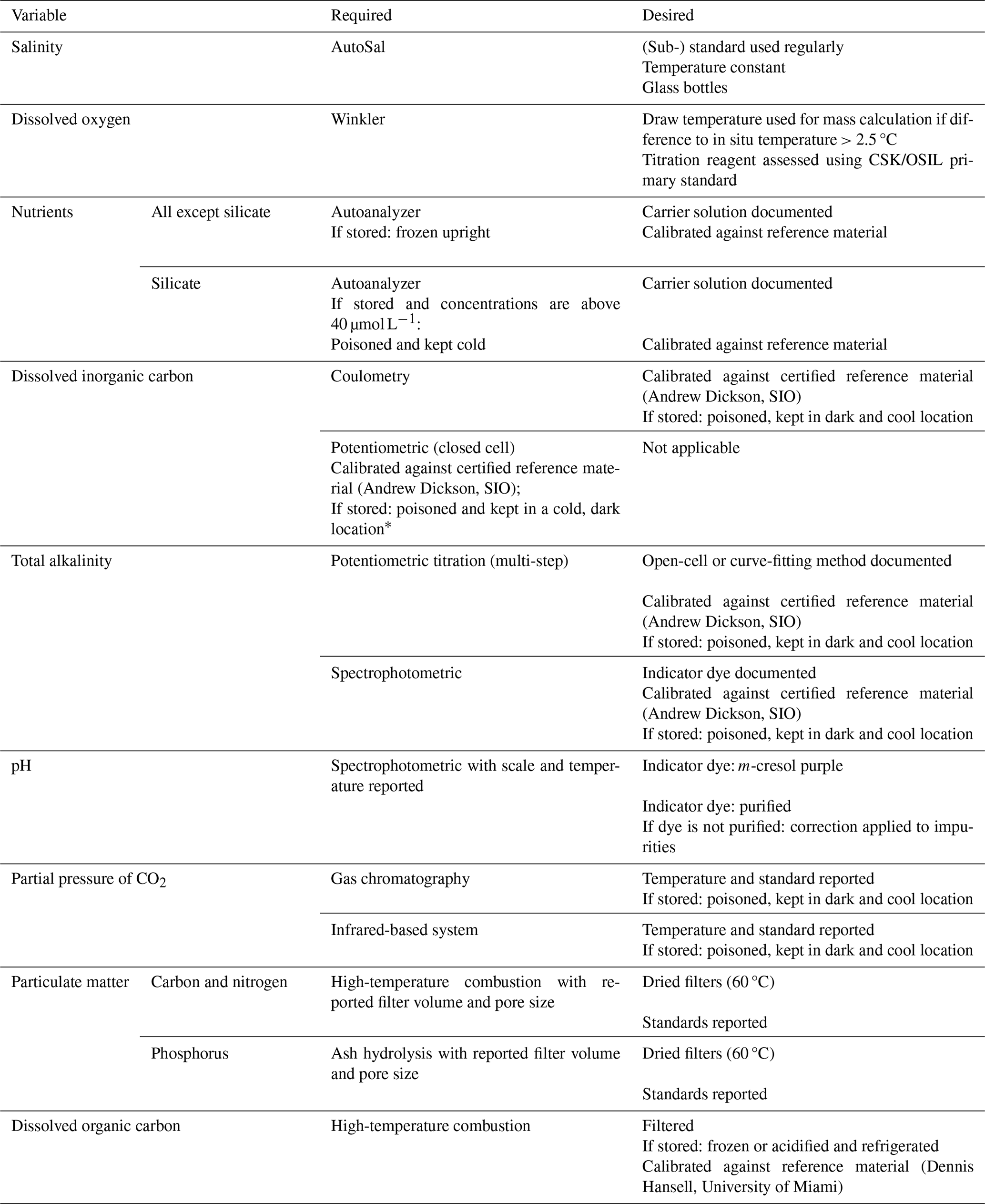
* Capped at a SOP flag 2.
3.4 Quantitative assessment of data
In addition to the qualitative method assessment (Sect. 3.3), the bottle data of the time series are described by our quantitative descriptors: (1) precision, (2) accuracy, (3) variability in the most consistent depth layer, and (4) consistency with GLODAP (Lauvset et al., 2022).
3.4.1 Precision and accuracy
Precision and accuracy estimates, as provided by each time-series program's primary quality assurance procedure, were assigned to the bottle data. The temporal resolution of these estimates varies from estimates given for each cruise, i.e., on a cruise-to-cruise basis, to estimates given for longer time periods (covering multiple cruises) without recorded changes in the applied methodology (Table S6), depending on the individual time series' internal procedure. If only one estimate was given for a variable for the entire time series, that estimate was only assigned to the most recently applied method. The units correspond to the units of the respective variable.
Precision estimates are based on replicate samples and are expressed as 1 standard deviation of the replicate measurements3. For the inorganic carbon variables, the assigned accuracy estimates represent the deviation from certified reference materials from the A. Dickson Laboratory (Scripps Institution of Oceanography). The pH accuracies of RADCOR are an exception, representing the difference from the theoretical TRIS buffer value at 25 °C. For oxygen concentrations, the assigned accuracy estimates represent the accuracy of the KIO3 primary standard normality assessed using a certified reference standard from either Ocean Scientific International Ltd (OSIL) or Wako Pure Chemical Industries (WAKO). For nutrient concentrations, the assigned accuracy estimates represent the deviation from the reference material from either OSIL, WAKO, or QUASIMEME (Wells and Cofino, 1997) or from the certified reference material from Kanso Technos Co., Ltd (KANSO). For total particulate phosphorus concentrations, the assigned accuracy estimates represent deviations from National Institute of Science and Technology (NIST) apple leaves (0.159 % P by weight). For DOC, the accuracy estimates represent deviations from deep seawater reference material from Dennis Hansell (RSMAS, University of Miami). The exact calculations to express the above deviations from reference materials differ slightly across the time-series programs (Table S7), thereby preventing combined precision and accuracy estimates to calculate a total uncertainty in a consistent manner. The estimates should not be confused with values provided by instrument manufacturers, which are ideal values and are usually well below real-world uncertainties.
3.4.2 Minimum variability
To provide an internal consistency measure of measurement quality, we determined the minimum variability of each BGC variable for each time-series station on the pressure surface (±100 dbar) with the least oxygen variability, i.e., the layer on which oxygen has the lowest coefficient of variation. We chose oxygen as natural variability in oxygen can be linked to either variations in ventilation, water mass changes, or changes in consumption and production by biological activity4 (Sarmiento and Gruber, 2006; Keeling et al., 2010; Stramma and Schmidtko, 2019). As these natural oxygen changes are likely to be accompanied by changes in other BGC variables, we used the layer that is closest to an oxygen equilibrium as an approximation for the least natural variability in ocean BGC. In addition, this choice allowed us to use the salinity variability as an independent indicator of natural variability. For (i) CARIACO, (ii) GIFT, (iii) Munida, and (iv) RADCOR, this layer could not be determined properly, respectively, due to (i) anoxic water masses below the mixed layer, (ii) varying measurement depths, (iii) no oxygen data, and (iv) a shallow bottom depth of 80 m. The minimum variabilities of the other variables were subsequently determined by calculating the coefficient of variation of all samples on the identified pressure surface. A minimum of 10 samples on the pressure surface was required.
3.4.3 Comparisons to GLODAP
The final quantitative descriptor indicates how well the time-series data compare to the GLODAP dataset (GLODAPv2.2021, Lauvset et al., 2021) and vice versa, with no a priori assumption as to which is “correct”. To this end, we applied an adapted version of the GLODAP crossover routine to all individual cruises of the time-series programs. Generally, the crossover routine calculates a depth-independent offset between a cruise and a reference dataset based on multiple crossing cruises, i.e., crossover pairs. The secondary quality control of GLODAP depends heavily on this routine to determine and correct for biases of new cruises, which results in the high internal consistency of the core GLODAP variables. In the following, we first describe the crossover routine of GLODAP in detail and subsequently highlight the modifications applied to the routine so that it fits our pilot product's needs.
For a given variable, the depth-independent offset of a new cruise against GLODAP is calculated using the following steps:
-
Step (1). Detect all GLODAP cruises that cross the to-be-compared cruise (denoted as cruise A in the following), i.e., find all crossover pairs of cruise A in GLODAP. In the second QC of GLODAP, a crossover pair is defined by two cruises that have (at least) three stations within a 2° radius that include (at least) three samples below a minimum of 1500 dbar. These requirements ensure that the influence of natural signals on the calculated offsets is limited. That becomes especially important if the time period between cruise A and a crossing GLODAP cruise (denoted as cruise B in the following) is large.
-
Step (2). Interpolate the samples of cruise A and cruise B to the same standard depths. Usually, the concentrations are compared on sigma-4 surfaces5. Samples above the chosen minimum depth are ignored to exclude layers that are influenced by daily to interannual variability.
-
Step (3). Compare all existing samples of cruises A and B that are at the same depth surface and from stations within 2°. For each depth surface, the individual offsets are averaged to obtain depth-dependent mean offsets and standard deviations. For nutrients and oxygen, the offsets are multiplicative, and for the carbon variables and salinity, the offsets are additive.
-
Step (4). Calculate the constant offset of cruise A against cruise B by inverse variance weighting all depth-dependent offsets. The resultant depth-independent offset is also known as the crossover-pair offset.
-
Step (5). Calculate the standard deviation of the crossover-pair offset by inverse variance weighting all depth-dependent standard deviations. This crossover-pair standard deviation reflects the similarity of the offsets within one depth surface and across all depth surfaces. The lower it is, the higher the confidence in the crossover-pair offset.
-
Step (6). Repeat steps (2) to (5) for all identified crossover pairs.
-
Step (7). Calculate the total offset of cruise A against GLODAP by inverse variance weighting all calculated crossover-pair offsets. The resultant standard deviation describes the overall uncertainty in the total offset.
For our purposes, we applied an adapted version of the above-described crossover routine using GLODAP as the “reference dataset” against which each time-series station is compared. The term reference dataset does not imply that the quality of GLODAP is higher than the quality of the time-series programs, only that it represents a dataset with known consistency in time and space. Each cruise of a time-series station, i.e., station visit, represents another cruise A in the above-outlined crossover steps.
For a given time-series station and variable, our adapted crossover routine starts with the identification of crossover pairs for each station visit, similarly to step 1. However, since multiple time-series cruises only take one profile with fewer than three samples below 1500 dbar, we could not apply the same crossover-pair requirements. We kept the distance requirement of 2° and added a new temporal requirement that only crossover cruises within ±45 d were included in the routine. That permitted relaxing the minimum depth requirement and dropping the requirement of the minimum number of profiles. Table 5 lists the corresponding layer depths (for the samples being used in the crossover analysis) for each time-series site. Note that we excluded crossover pairs of cruises that are included in both products (parts of IC-TS, IRM-TS, and OWSM). Steps 2 to 6 of the routine are identical and repeated for all time-series station cruises. In the next step, all crossover-pair offsets against the same GLODAP cruise, i.e., a particular cruise B, are averaged. This step was necessary when multiple time-series cruises took place within 90 d and were all compared to the same cruise B. Consequently, we obtained one depth-independent offset (and standard deviation) of the time-series station against each GLODAP cruise that meets the crossing requirements. In a final calculation, we determine the total offset of the time-series station against GLODAP by inverse variance weighting all obtained time-series station offsets. If the standard deviation of the time-series station offset against a particular cruise B was below the consistency estimates of GLODAPv2 (see Table 11 in Olsen et al., 2016), the latter ones were used as standard deviations (for example, only one crossover pair exists between the entire time series and a particular cruise B). The routine was only applied to variables defined as core variables6 in GLODAP. Negative (or lower-than-unity) offsets indicate lower values compared to GLODAP and vice versa.
4.1 Method evaluation
The results of the method assessment indicate that the time-series programs have documented their methodology well and that the most recent methods generally follow recommendations by prevalent initiatives in the field (Fig. 3 and Table 3). The proportion of data allocated a SOP flag 1 is strongly dependent on the variable and program assessed. The assigned flags partly reflect that, over the 40 years, multiple method changes occurred (Fig. 4). Method changes are even more pronounced in programs without a dedicated vessel (Table 1). However, not all changes are captured by the assigned SOP flags, e.g., instrument changes (Table S6). Note that the overall percentages in Fig. 3 are skewed towards ALOHA as the number of ALOHA samples makes up around 60 % of all samples of the product (Sect. 5).
Further, note that SOPs are constantly evolving, and, consequently, this assessment must be seen as dynamical. In some cases, programs explicitly choose to not follow the most recent recommendations in favor of method consistency. For example, unpublished internal analyses and discussions in the HOT program about possible advantages and disadvantages of a purified dye for the pH measurements (recommended following the Bermuda Time Series Workshop report) resulted in not changing their dye. These additional analyses demonstrate the difficulties in determining SOPs, but the knowledge is often not shared with the wider community. Hence, regular time-series workshops that discuss currently applied methodologies, achieve community consensus, and result in method recommendations that are implemented accordingly in the here-applied assessment should take place regularly.
In the following, the results will briefly be presented for each assessed variable.
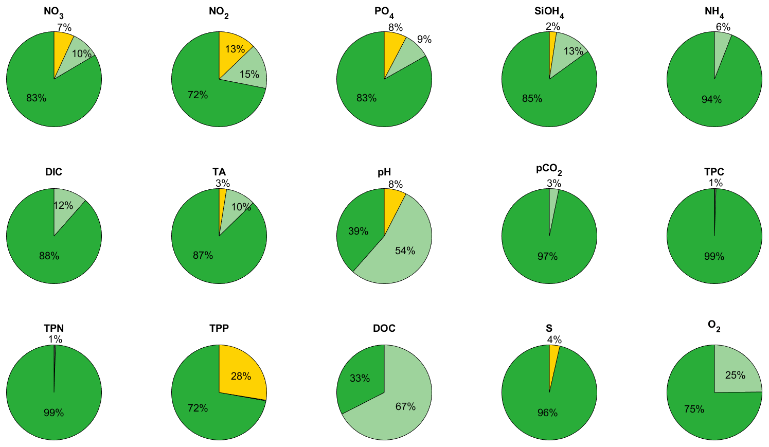
Figure 3Overview of assigned SOP flags. Percentages correspond to the number of samples in the combined dataset. Dark-green colors indicate samples that have been measured according to all (including desired) SOP requirements, i.e., a SOP flag 1 (Table 2). Light-green colors indicate samples that have been measured meeting the required SOP requirements only, i.e., a SOP flag 2. Orange colors indicate samples for which the methods do not meet the SOP requirements, i.e., a SOP flag 3. Variable synonyms correspond to the product header names (Table 1). Note that total particulate matter includes the exclusively organic particulate matter measurements from CVOO.
4.1.1 Salinity
For salinity, 96 % of the bottle samples meet all SOP criteria. DYFAMED, GIFT, Munida, and RADCOR only provided CTD salinity values and are not included in this statistic. The remaining 4 % of bottle salinity samples with a SOP flag 3 are from a few cruises of ALOHA and CVOO. Salinity samples of the first 26 cruises of ALOHA were measured using an AGE Minisal 2100 salinometer. Also, the first 23 cruises of ALOHA used plastic bottles (instead of glass bottles) to sample salinity, which made them more prone to evaporation. Note that the data were corrected for it. Further, measurements taken on CVOO's research vessel Islandia used a Micro-Salinometer MS-310 (RBR Ltd, Canada) instead of the up-to-now-required AutoSal (Guideline Instruments, Canada).
4.1.2 Oxygen
Even though the overall statistics show that 75 % of all bottle oxygen samples were measured according to the required SOPs, 6 out of the 11 programs (Munida time-series program does not measure oxygen) did not regularly use certified reference KIO3 (CSK, WAKO, OSIL) to assess the accuracy of the Winkler titration measurements. ALOHA, DYFAMED, GIFT, K2, KNOT, and RADCOR (as well as very few cruises from CVOO) used standard reference iodate. Further, note that, during the first 10 HOT cruises, the in situ temperature was used to calculate the mass rather than the sample draw temperature, resulting in a slightly negative bias which is reflected in a SOP flag 2 for the concerned oxygen samples. The Winkler end-point detection method was either visual (using starch as a color indicator) or computer-controlled potentiometric detection, both of which are accommodated in the applied method assessment.
4.1.3 Nutrients
In most cases, all nutrient variables were measured simultaneously using one water sample (and/or with replicates at a single depth sampled), and the applied methods were identical. This is represented in similar SOP flags of the nitrate, phosphate, and silicate samples. For these three variables, around 95 % of the applied methods met either all SOP requirements or the required requirements. The most restricting SOP requirement is the comparison to reference materials, which, especially for older datasets, was not met. The remaining data with a SOP flag 3 correspond to 2 % of the silicate, 7 % of the nitrate, and up to 8 % of the phosphate samples. These flags are linked to the preservation technique applied (poisoned instead of frozen for nitrate and phosphate), which particularly explains the lower fraction of silicate samples that do not fulfill the required criteria (DYFAMED, OWSM). Note that internal analyses at DYFAMED resulted in favoring poisoning nutrients for conservation over storing them frozen and that DYFAMED reversed back to the former method in 2012, as reflected in the large percentage of SOP flag 3. However, such insights were not integrated into this assessment and underpin the need for regular workshops discussing and updating SOP recommendations for ship-based time series. In this context, we want to mention the recently started Euro GO-SHIP project (https://eurogo-ship.eu/, last access: 3 April 2024) and, in particular, the related comparability assessment of different nutrient preservation protocols.
Nitrite and ammonium samples show slightly different patterns because the number of measured samples deviates from the above-described nutrients; i.e., the influence of the ALOHA nutrient samples is smaller.
Differences in the type of autoanalyzer (rapid-flow analyzer or continuous segmented flow), storage duration and temperature, defrost procedure, carrier solution (in-house artificial seawater that resembles the nutrient concentrations of the region, in-house low-nutrient seawater, or commercially available OSIL standard), reference material (WAKO, OSIL, KANSO), and sample filtering were not considered in the evaluation. Such differences can also occur in time within a time-series program, as shown for nitrate in Fig. 4. Note that the dependency of the CVOO time series on research vessels of opportunity results in multiple small methodological changes – e.g., to the instrument and sample volume and to whether the sample is analyzed at sea or stored frozen.
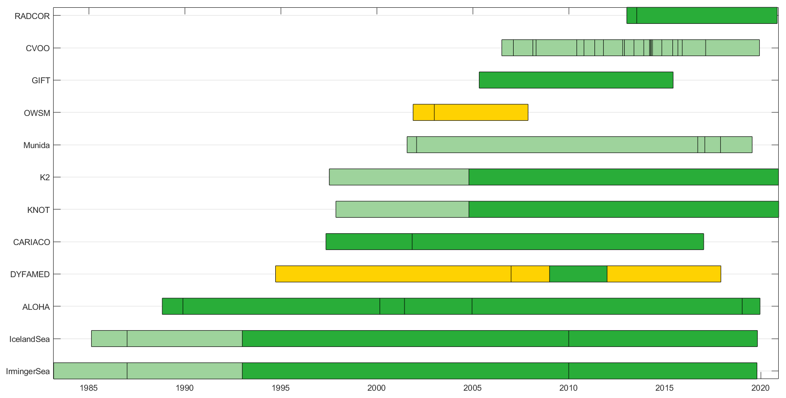
Figure 4Time dependency of assigned SOP flag of each time-series program exemplarily shown for nitrate. Vertical black lines indicate method changes both captured and not captured (e.g., instrument change) by the SOP flags. The color scheme used is identical to that in Fig. 3. Note that DYFAMED changed back to poisoning the samples for conservation based on internal analyses of conservation methods.
4.1.4 Dissolved inorganic carbon
For DIC, 88 % of the samples were measured according to all method recommendations. DYFAMED is the only time-series program that measures DIC potentiometrically in a closed cell. Even though DYFAMED has made use of Dickson's certified reference materials (CRMs) since 1999, closed-cell potentiometric measurements of DIC alone have an offset (1 %–2 % lower) (Bradshaw et al., 1981, and Millero et al., 1993), resulting in a SOP flag 2. The remaining samples that do not meet the desired SOP requirements are pre-1991 samples from ALOHA, IRM-TS, and IC-TS, for which certified reference material was unavailable, also resulting in a SOP flag 2.
Differences in sample storage duration and coulometer calibration methods (gas loop calibration or sodium carbonate solutions) were not considered in the evaluation. Very few samples for DIC are taken on the RADCOR cruises.
4.1.5 Total alkalinity
TA is one of the few variables measured by all participating time-series programs; 87 % of the samples met all SOP requirements, 10 % met the required requirements only, and 3 % did not meet the required recommendations. The latter correspond to cruises for which metadata on TA are not present (ALOHA cruises 1–22) and to cruises where TA was measured using a single-point titration (only a few cruises at DYFAMED, K2, and KNOT sites) (Fig. 5). The SOP flags of 2 are either linked to (i) missing information on the indicator, cell type, and/or curve-fitting method used or (ii) non-application of certified reference materials. Differences in storage duration, cell type, end-point, and curve-fitting method (least-squares or modified Gran functions) were not considered in the evaluation.
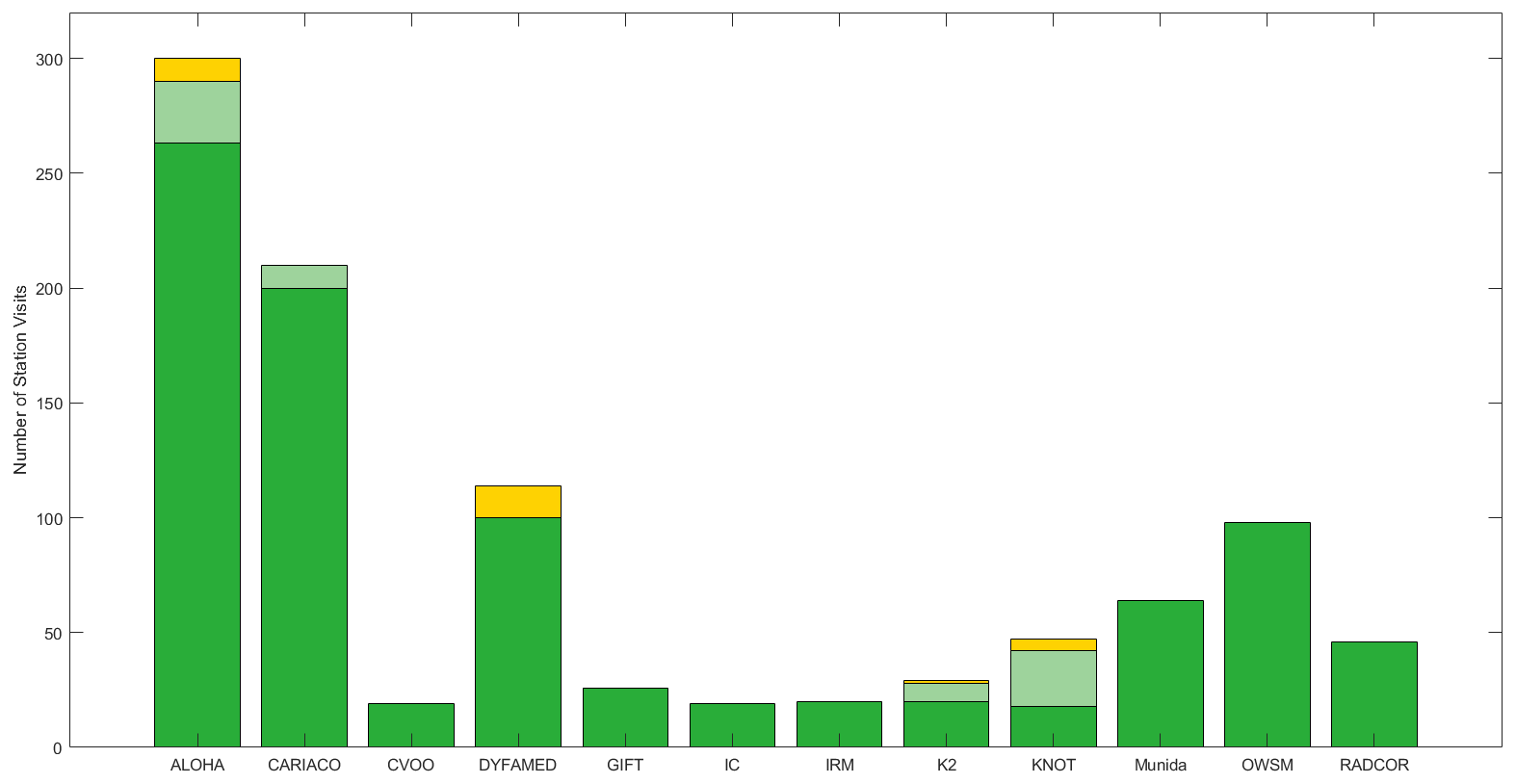
Figure 5Assigned SOP flags per station exemplarily shown for TA. Flags have been assigned on a cruise-per-cruise basis, i.e., per station visit. The color scheme used is identical to that in Fig. 3.
4.1.6 pH
Even though most programs which analyze pH follow the methodology of Clayton and Byrne (1993), pH has the lowest number of programs with methods meeting all the SOP requirements. CARIACO's protocol is the only one which meets all pH SOP requirements, as reflected in the overall percentage of samples with a SOP flag of 1 being only 39 %. ALOHA, GIFT, and RADCOR reported pH on the total scale at 25 °C and 0 dbar and analyzed pH using unpurified m-cresol purple. But none of these programs corrected for the impurities of the dye (54 % of the samples), thereby not meeting the SOP flag 1 criteria. A few cruises of DYFAMED, K2, and KNOT measured pH, but pH was measured potentiometrically (less stable and accurate; Lorenzoni and Benway, 2013).
Differences in the storage duration and, more importantly, whether an additional correction for pK* of the indicator dye m-cresol purple was applied (suggested by DelValls and Dickson, 1998) were not part of the SOP flag evaluation. The latter correction has been applied by GIFT and CARIACO.
4.1.7 Partial pressure of CO2
The only two time-series programs that measure partial pressure of CO2 (pCO2) are the IRM-TS and IC-TS, both being measured by the same personnel using identical protocols. The presently applied protocol meets all SOP requirements. Before mid-1993, the samples (3 % of the total) were not poisoned for storage, but, instead, equilibrated gas was isolated and sealed in a 300 mL glass flask. Further temporal changes in the methodology are explained in Olafsson et al. (2010).
4.1.8 Particulate matter
Particulate matter concentrations are only measured at ALOHA, CARIACO, and CVOO, with CVOO being the only station that fumes the dried particulate matter filters with concentrated hydrochloric acid, thereby removing the inorganic carbon components; i.e., CVOO is the only station that measures particulate organic matter only. Note, however, that, at CARIACO, inorganic components of carbon (nitrogen) particulate matter are assumed to contribute insignificantly to the overall total concentrations. ALOHA and CARIACO meet all SOP requirements for total particulate carbon and nitrogen, whereas CVOO (< 1 % of all samples) is missing information on the standards used. ALOHA's total particulate phosphorus measurements (75 % of all samples) also meet all SOP requirements, but CARIACO's metadata do not include details on the filter used for these measurements. CVOO also lacks detailed metadata for particulate organic phosphorus.
Differences in storage duration and, more importantly, filter sizes and types, heating temperature and duration, and leaching time were not part of the evaluation. According to ALOHA's protocols, differences in the latter resulted in large variations in the measured total particulate phosphorus content. ALOHA total particulate phosphorus samples pre-2012 are biased low.
4.1.9 Dissolved organic carbon (DOC)
ALOHA, CARIACO, GIFT, and K2 have measured DOC, and the samples of CARIACO, GIFT, and K2 have been filtered. Thus, 33 % of the DOC samples have a SOP flag 1, and all samples from ALOHA (67 %) received a SOP flag 2.
4.2 Minimum variability
The layers with the lowest oxygen variability (0.7 %–3.4 %) are all located below 1000 dbar and represent the bottom layer in the cases of ALOHA, DYFAMED, and the IRM-TS (Table 4). For CVOO, IC-TS, K2, and OWSM, the determined layers are near-bottom to intermediate layers, probably reflecting that oxygen concentrations at the bottom are more prone to boundary layer effects in these regions. At KNOT, we can link this layer to the continual influx of NPDW.
Salinity shows the lowest variability for all time-series stations, ranging from 0.003 % to 0.086 %. The higher values indicate that natural variability likely had a strong influence on the calculated numbers. Silicate is generally the nutrient with the highest variability within and across the time-series programs, with the IRM-TS experiencing the highest variability (6.7 %). Such a high coefficient of variation cannot solely be linked to large uncertainties in the measurements (silicate accuracies (Vcrm) at the IRM-TS are around 3.5 %). Hence, natural variabilities in the nutrients are very high in this region in the determined layer, which also corresponds with the upper end of the salinity (and temperature) variability. Nonetheless, silicate, having the highest of all nutrient variabilities, fits well to the assigned accuracy values and also to previous findings of rather high uncertainties in silicate concentrations (e.g., inter-laboratory studies described in Bakker et al., 2016b) and experiences from the GLODAP quality control (Olsen et al., 2016). The coefficients of variation of DIC and TA are below 0.5 % for all time-series stations, with a maximum of 0.4 % (around 9 µmol kg−1) at DYFAMED and a minimum of 0.1 % (around 2 µmol kg−1) at ALOHA, K2, KNOT, and CVOO. The latter are within the provided accuracy estimates and indicate very constant DIC and TA data quality. Minimum pH variability could only be calculated for ALOHA (0.04 %), which is in the range of the provided pH precision values at ALOHA. DOC variabilities could be calculated for ALOHA and K2. For the former, it is 8.5 % and thus around twice as large as the given accuracy and precision values. For the latter, it is 1.7 % and fits very well with the provided precision values. For the IRM-TS and IC-TS pCO2 data, the determined coefficients of variation are 2 to 3 times as large as the stated precision (Olafsson et al., 2010), which again can be linked to the rather high natural variability of all variables at these stations. No minimum consistencies could be calculated for particulate matter.
The obtained minimum variabilities can, in some cases (e.g., ALOHA), be cautiously interpreted as an inter-consistency determination of the measurement quality. In these cases, low variability indicates a consistent level of data quality throughout the measurement period. A high variability then likely indicates a variable level of data quality. Here, the determined layers can also be used to detect suspicious samples. However, some sites are characterized by large natural variability on all depth surfaces (on several timescales), likely accompanied and recognizable by high salinity and temperature variability. For these stations (IRM-TS, IC-TS, DYFAMED), the high variability estimates should not be confused with a high variability in measurement quality.
Table 4Minimum variability expressed as the coefficient of variation (%), except for temperature. Here, the standard deviations is given instead (in °C) as mean temperatures being very close to zero and/or negative resulted in misleading coefficients of variation. The corresponding layer depth of the layer with the least oxygen variability (±100 dbar), on which the variabilities have been calculated, is shown too. The variable abbreviations are the same as in Table 1. The asterisk denotes that CTD salinity values have been used for the calculation. NA denotes not available.
4.3 Comparison to GLODAP
The relaxation of the crossover analysis (Sect. 3.4.3) enabled the determination of the offsets between GLODAP and the time-series stations of ALOHA, CVOO, IC-TS, IRM-TS, KNOT, K2, and OWSM (Table 5). Generally, the analysis indicates a very good fit between the SPOTS pilot and GLODAP at these sites. Significant offsets suggest the potential for bias in either the SPOTS pilot or GLODAP, but further analysis of both products is required to assess the source of the bias. In the following, the results are presented for each time-series program individually.
Table 5Mean offsets (rounded) of the SPOTS pilot against GLODAP core variables. The first number in parentheses shows the number of cruises from the time-series program compared to GLODAP. The second number in the parentheses shows the total number of cruises from GLODAP to which the time-series cruises are compared. The variable abbreviations are the same as in Table 1. a denotes whenever the crossover analyses have been performed on pressure surfaces. b denotes that CTD values have been used for the calculation. NPDW stands for North Pacific Deep Water. NA denotes not available.
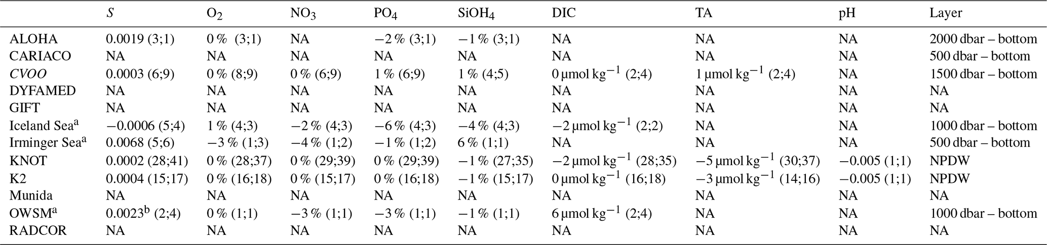
4.3.1 ALOHA
For ALOHA, all calculated crossover offsets fall within the provided GLODAP consistencies (Lauvset et al., 2021), indicating a good fit between the two products. There are no crossover cruises for nitrate and carbon variables. Further, only three ALOHA cruises (HOT174–HOT176) are compared against only one GLODAP cruise (49NZ20051031) as these are the only crossover pairs that meet the crossover criteria. Note that 49NZ20051031 has passed the full second QC of GLODAP and that the individual crossover-pair offsets are similar. Nonetheless, the small number of underlying data strongly reduces the confidence in the results.
4.3.2 CVOO
Crossover offsets could be calculated for all GLODAP core variables which were measured at CVOO. All analyzed variables fall clearly within the provided GLODAP consistencies, indicating a good fit between the two products at CVOO. The results are robust, given the number of CVOO cruises compared to GLODAP. Further, there is very good agreement between the individual crossovers, i.e., low standard deviations of the individual offset between one cruise and GLODAP, and consistency among all CVOO cruise offsets, with no large outliers. Data from a few cruises are present in both products.
4.3.3 Iceland Sea
The crossover offsets of the IC-TS of salinity, oxygen, nitrate, and DIC against GLODAP are within the consistency limits of GLODAP; i.e., no significant offset is remarkable between the two products. For nitrate, the variability between the individual offsets is large, which reduces confidence in the analysis. For phosphate, the SPOTS pilot has 6 % lower concentrations than GLODAP based upon four cruises from the IC-TS (B17-94, B9-96, B12-96, and B5-2002) and three GLODAP cruises (58JH19941028, 58JH19961030, and 316N20020530), which all passed GLODAP's second QC. This large offset mainly originates from the 2002 cruise, while cruises from 1996 indicate a good fit. The same cruises show a −4 % offset for silicate, and the underlying data show a similar pattern. However, the relatively large minimum variability of salinity (Sect. 4.2) demonstrates that the Iceland Sea is a dynamically active region with deep open-ocean convection and complex seasonally varying currents; this high natural variability reduces confidence in the crossover analysis for the Iceland Sea region.
4.3.4 Irminger Sea
All crossover offsets of the IRM-TS against GLODAP are above GLODAP's consistency limits, except for phosphate. However, given (i) that the minimum depth had to be set to only 500 m in a deep-water-formation area and (ii) the relatively large minimum variability of salinity (Sect. 4.2), the larger offsets were expected and are likely attributable to the inherent natural variability of this region. Further, the relatively small number of crossovers does not allow for a more in-depth investigation of the offsets.
4.3.5 KNOT
Crossover offsets could be calculated for all GLODAP core variables. The calculations were performed on the NPDW, which has a residence time of about 500 years (Stuiver et al., 1983). Following the definition from Wakita et al. (2010), we used 27.69σ (around 2000 dbar) and 27.77σ (around 3500 dbar) as limits. All of the so-calculated offsets of KNOT against GLODAP are clearly within the consistency limits, except for TA (−5 µmol kg−1). Confidence in the analysis is provided through a large number of crossover cruises and consistency in the calculated offsets. Data from a few cruises are present in both products.
4.3.6 K2
Crossover offsets could be calculated for all GLODAP core variables. The calculations were again performed on the NPDW using limits identical to those of KNOT. All of the so-calculated offsets of K2 against GLODAP are clearly within the consistency limits. Confidence in the analysis is provided through a large number of crossover cruises and consistency in the calculated offsets, as exemplarily shown for nitrate (Fig. 6). Data from a few cruises are present in both products.
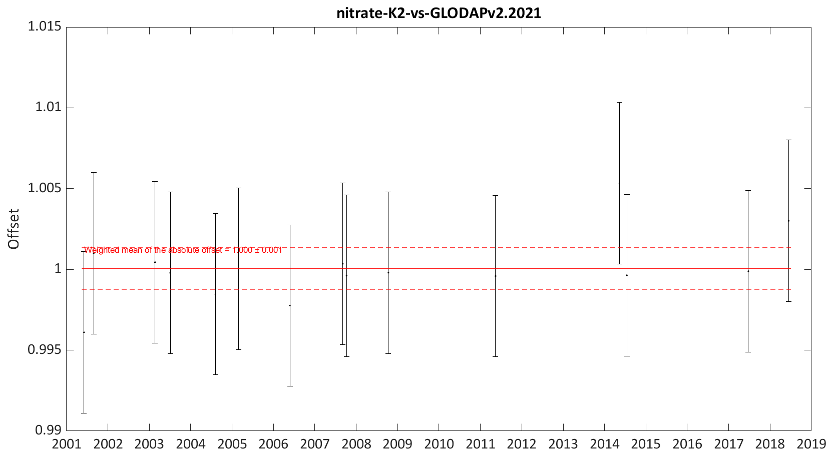
Figure 6Total weighted offset of the SPOTS pilot nitrate data against GLODAPv2.2021 at station K2 in the North Pacific Deep Water (NPDW) layer. The total weighted offset is multiplicative and illustrated by the red line (here equal to 1.00, i.e., no offset). The dashed red lines are the corresponding standard deviation. The black dots display the weighted offsets of individual K2 cruises against GLODAP cruises, with the corresponding error bars displaying their standard deviation. If the calculated standard deviation of the individual cruises is lower than GLODAP's nitrate consistency limit (2 %), it is set to the latter. The summary figure indicates a very good fit between the SPOTS pilot product and GLODAP at the K2 station for nitrate, with a total weighted offset of 0.0 %.
4.3.7 OWSM
Crossover offsets at OWSM indicate slight mismatches between the nitrate, phosphate, and DIC concentrations of the SPOTS pilot vs. GLODAP. The total weighted mean offsets are −3 %, −3 %, and 6 µmol kg−1, respectively. The former two offsets are only based upon a comparison between the OWSM cruise from 15 April 2002 (no CRUISE ID present) and 316N20020530. Three more recent OWSM cruises from 2019 are additionally checked against 58JH20190515. Both GLODAP cruises passed GLODAP's second QC. However, the DIC offsets are very dependent on the crossover pair, and the final offset should be treated with caution. The small number of crossovers does not allow for a more in-depth investigation of the relatively small offsets.
The product file variable names are described in Table S8. Each fixed-location time-series station is identified by the entry under TimeSeriesSite, and individual cruises are identified by CRUISE. Station, cast, and bottle numbers are linked to the original cruise campaign numbering (if provided). In some cases, station number duplicates within the same time-series program exist as the data originate from different research vessels of opportunity (Table 1). Nitrate values can contain nitrite concentrations (Table S4). Since all pH values were reported on the total scale at 25 °C, no additional pH temperature entry is provided. Conversely, for pCO2, corresponding temperature measurements are given. In addition to the WOCE flags, each bottle variable is further accompanied by the assigned SOP Flag (Sect. 4.1) and by the provided precision and accuracy estimates (Sect. 3.4.1). The last column lists the digital object identifier (DOI) of the original dataset. All missing entries are indicated by −999.
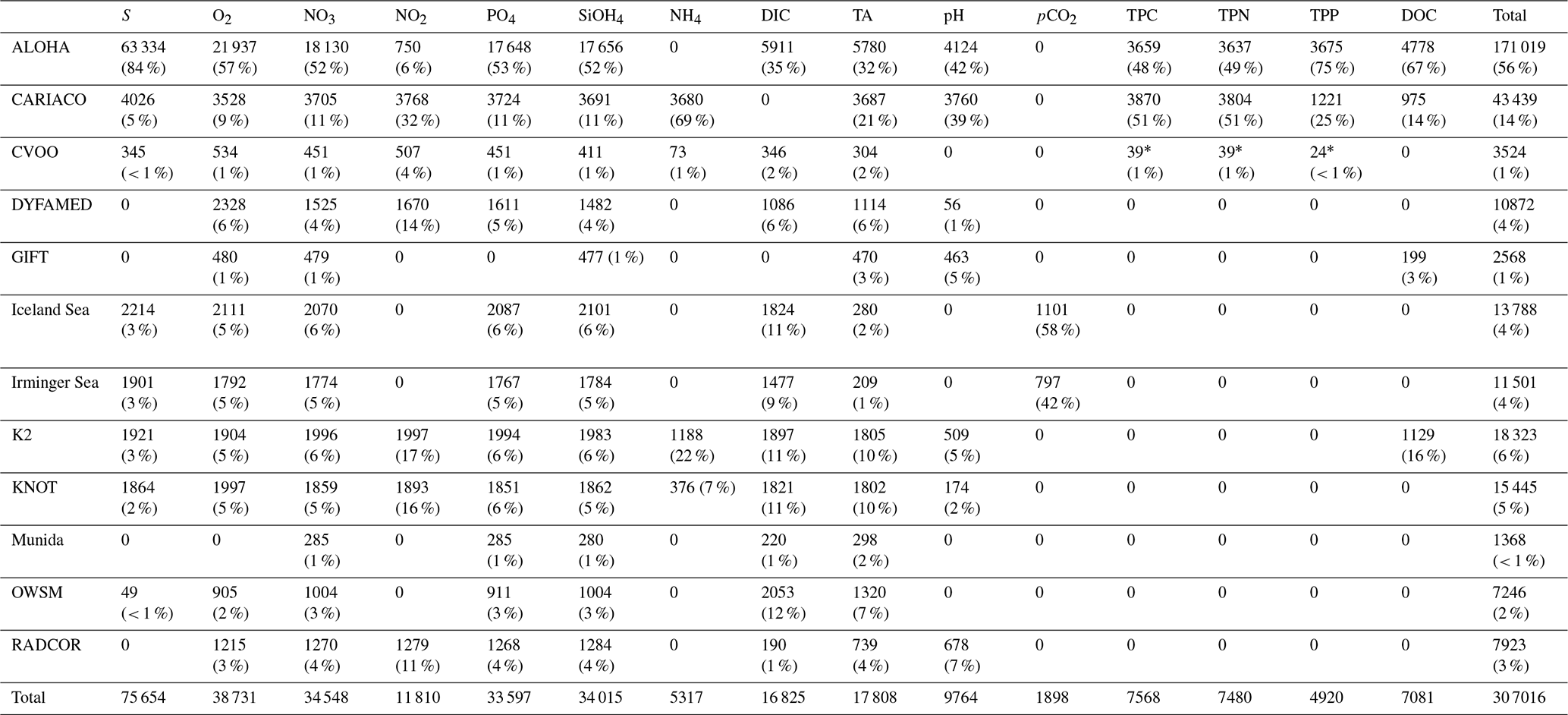
A total of 108 332 water samples are included in the product. Bottle salinity with 75 654 measurements is the variable with the most abundant data (Table 6). The number of bottle salinity samples is about twice the number of bottle oxygen and nutrient (excluding ammonium and nitrite) samples and almost 5 times the number of included DIC and TA samples; pH and nitrite have around 10 000 samples, and the product includes between 4900 and 7600 samples of particulate matter, DOC, and ammonium. With 1898 samples from the IRM-TS and the IC-TS, pCO2 is the variable with the fewest measurements. Silicate, nitrate, and TA are the only variables measured at all sites. Around 56 % of all bottle data values originate from ALOHA (Table 6), and 14 % originate from CARIACO. The remaining 25 % are distributed rather equally across the different programs. ALOHA's large percentage can be explained by measurements at ALOHA (i) having taken place consistently on a monthly basis for ≥ 30 years, (ii) including up to 30 hydrocasts per station visit, and (iii) including all but two of the product's bottle variables. The dominance of ALOHA's measurements is most pronounced for salinity, total particulate phosphate, and DOC (around 70 %–80 % of the samples are measured at ALOHA). For oxygen and nutrients, ALOHA's samples represent around 52 % of all samples, and for the inorganic carbon variables (DIC, TA, and pH), they represent between 32 %–42 %.
Table 6Summary statistics showing the total number of samples per variable included in the SPOTS pilot of each time-series site. Percentages in brackets show fractions in comparison to the total number per variable, except for the last column. Percentages are rounded; thus, the sum is not always equal to exactly 100 %. Variable abbreviations are identical to Table 1. The asterisk denotes that CVOO measures particulate organic matter only even though, here, these were counted towards total particulate matter measurements for a better overview.
The main stakeholder groups of SPOTS are the data providers on the upstream end, i.e., the individual time-series programs (Sect. 2), and users of time-series data on the downstream end. Regarding the latter, the SPOTS pilot is intended to be applied in different ocean BGC fields: evaluations of ocean BGC; neural networks such as CANYON-B (Bittig et al., 2018), CANYON-MED (Fourrier et al. 2020), or ESPER (Carter et al., 2021); regional ocean BGC models (e.g., models participating in RECCAP, such as that of Ishii et al., 2014); 1D model applications (e.g., Mamnun et al., 2022, using REcoM2); global ocean BGC models participating in model intercomparison projects (e.g., Coupled Model Intercomparison Project – Orr et al., 2017); evaluations of autonomous BGC observing networks such as BGC Argo (Bittig et al., 2019); global scientific assessments such as the Global Carbon Budget (Friedlingstein et al., 2022); or multi-time-series studies and analyses (e.g., Bates et al., 2014; O'Brien et al., 2017). These time series can also contribute ocean carbonate chemistry data to the United Nations Sustainable Development Goals, especially target 14.3 (to minimize and address the impacts of ocean acidification).
6.1 Benefits
The main goal of SPOTS is that both stakeholder groups benefit from the product. Through a use case, the benefits for the users are demonstrated in Sect. 6.2.
Upstream, data providers benefit from the product through (1) increased impact of individual ship-based time-series programs and (2) increased visibility and discoverability, particularly of smaller and less well-known time-series programs. Here, two “pull factors” contribute: (i) the linking of all time-series data with the data of larger time-series programs and (ii) being exposed to global data systems through the Ocean Data and Information System (ODIS), coordinated by IOC-UNESCO (https://book.oceaninfohub.org, last access 3 April 2024) (Sect. 7.2). The larger sites also benefit from the latter, but the impact of larger time-series programs is, in particular, increased through enhanced usability of their data. Here, the proverb “the whole is greater than the sum of its parts” perfectly describes the benefits of SPOTS. The envisioned (non-exhaustive) list of users underscores the idea that consistent and inter-comparable data from multiple time-series programs (i.e., the whole) lead to an extended range of applications relative to the data of a single time-series program. The data being automatically uploaded to ERDDAP (Environmental Research Division's Data Access Program), which increases the accessibility, interoperability, and machine-readability (Sect. 7.2), also becomes important in broadening the users and applications of data from these time-series programs.
Further, participating time-series programs benefit from optional data management support for formatting, QC, and data archival. This support aims to reduce the data management workload of individual programs and being directly ascribed to the FAIR data practices. Regarding guidelines and SOPs, the participating time-series programs also benefit from the product fostering collaborations across several programs, which is especially relevant for emerging time-series programs.
The product contributes to the development of a sustained, globally distributed network of time-series observatories that sample a core set of biogeochemical and ecological variables guided by common SOPs (methodological, FAIR data, etc.). These are required attributes of a GOOS observing network, and achieving this status (possibly as a sub-network of OceanSites) would ultimately help position ship-based time-series programs for expansion under the United Nations Decade of Ocean Science umbrella. In addition, the product links individual time-series efforts to larger policy directives such as the Marine Strategy Directive Framework in Europe with respect to, e.g., ocean monitoring indicators.
6.2 Use case
As an example to demonstrate both the utility and potential misuses of the SPOTS pilot, we applied the recently developed Trends of Ocean Acidification Time Series software (TOATS, https://github.com/NOAA-PMEL/TOATS, last access 3 April 2024) to the mixed-layer TA data included in the product (Fig. 7). The TOATS software is a supplement to the recently published best practices for assessing trends of ocean acidification time series and provides a Python-based Jupyter Notebook to compare trends across different (BGC) time-series datasets (Sutton et al., 2022). It was developed based on several published trend analysis techniques to standardize estimating and reporting trends from ocean carbon time-series datasets. Following a strict methodological analysis7, TOATS estimates (i) the linear trend, (ii) its uncertainties, and (iii) the trend detection time of the assessed time-series data. The latter indicates the minimum observational period needed to statistically distinguish between natural variability (noise) and anthropogenic forcing. This method requires time series with a sub-seasonal sampling frequency to constrain the seasonal variability of surface ocean carbonate chemistry; however, for the purpose of this example, we assessed all time-series programs rather than restricting the assessment to time-series datasets with regular monthly measurements. The only non-trivial calculation step we applied before running TOATS was to calculate the surface mixed-layer depth for each cruise (defined using a 0.3 potential density anomaly criteria, following de Boyer Montégut et al., 2004) and to average TA concentrations within the estimated mixed layers. The results of our use case (Fig. 7) show trends in alkalinity for all time series (seven of them with significant trends).
The ease of use in applying TOATS to multiple time series simultaneously demonstrates the main benefits and potential misuse of the SPOTS pilot. Concerning the benefits, the combination of the SPOTS pilot and TOATS enables any user to perform joint time-series studies that follow published SOPs without requiring any in-depth digital knowledge. The need to, a priori, know about existing time-series program data and to subsequently mine, format, and QC the data is either mitigated or removed for all time-series datasets included in SPOTS. The required input format of TOATS is also readily available by accessing the time-series product data through ERDDAP (Sect. 7.2). Further, the linked open data structure of the data product allows detailed information on methods and their changes over time to be readily exposed through systems such as ODIS and to be delivered to users through portals such as IODE's Ocean InfoHub (2022, https://oceaninfohub.org/, last access 3 April 2024). This will enable a sophisticated information-driven data selection of (subsets of) time-series data to analyze the effects of method changes on detected trends without having to study multiple cruise reports. A similar advantage is provided through the possibility of selecting subsets of data based on the assigned SOP flags (Sect. 4.1). Lastly, the estimates of precision and accuracy included in the SPOTS pilot (Sect. 3.4) additionally enable confident uncertainty estimations of the trend analyses (uncertainties of the observations being a mandatory input in TOATS).
Regarding the potential misuse of the SPOTS pilot, caution must be applied in interpreting the results, particularly because the use-case analysis includes values accompanied by SOP flags 2 and 3. Simply assuming that the determined trends (Fig. 7) are valid and interpreting differences across time-series programs could lead to false conclusions. Robust trend analysis also requires the user to acknowledge the impact of large data gaps in time series that inhibit the ability to constrain seasonal variability in many of the included datasets (e.g., CVOO) and make it impossible to remove periodic signals with confidence (second step of TOATS trend analysis). Following TOATS guidelines, we recommend applying TOATS to surface ocean biogeochemical data with at least regular seasonal measurements or to restrict the trend analysis to specific seasons. Increasing the number of samples using additional interpolation and computational techniques could relax this restriction (e.g., multivariate linear regression; Vance et al., 2022), but computations accompanied by large uncertainties might also harm the robustness of the trend analyses. Note that, in the case of interpolating concentrations of single variables vertically, we recommend using a quasi-Hermitian piecewise polynomial (Key et al., 2010). And if techniques to increase the data coverage involve using CO2SYS (van Heuven et al., 2011), we recommend explicitly stating the used carbonate dissociation constants, the bisulfate dissociation constant, and the borate-to-salinity ratio.
Another large pitfall is neglecting the provided metadata and assuming that restricting the analyses to time-series data with a SOP flag 1 erases all artifacts in the trend analyses. Such a restriction would increase the robustness of the analysis, but unaccounted differences within the SOP flag 1 (Sect. 4.1) would still bias the results. For example, ALOHA total particulate phosphorus samples analyzed before 2012 are biased low but still fulfill all assessed SOP requirements (Sect. 4.1). Similarly, some standardizations of the product resulted in the neglect of valuable time-series details (e.g., information on ventilation events provided through the unique QC flags of CARIACO (Sect. 3.2)). We included all information in the additional metadata, made it easily accessible, and encourage users consult it, particularly to check for any correlations of the trend analyses to method changes (Table S6) and/or specific time-series events.
Even though this example highlights a multiple-time-series study use case, it depicts the benefits and, especially, the potential misuses for other applications of the SPOTS pilot. If the limitations of the product (e.g., data gaps and varying baselines) are acknowledged, quality descriptors are utilized, and the data are used in conjunction with the supporting metadata, multiple applications can benefit from this time-series product.
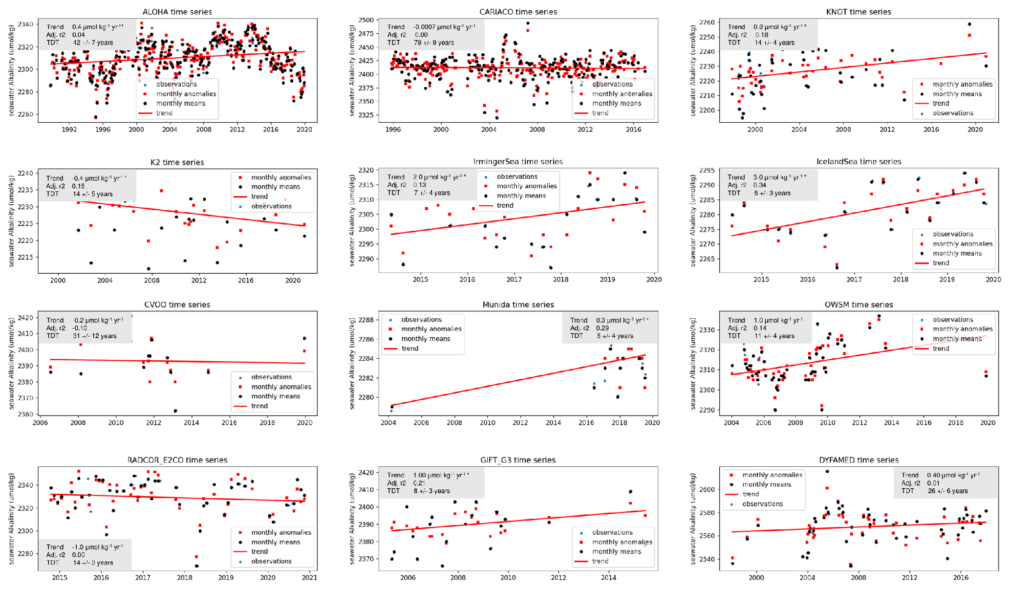
Figure 7Trend analysis of TA in the mixed layer using TOATS. Data symbols show the original time-series observations (blue circles), the time series of monthly means (black circles), the de-seasoned monthly means (red squares), and the trend of the de-seasoned monthly means (red line) (From Sutton et al., 2022). The monthly anomalies (red squares) that are used for the trend analyses are shown as de-seasoned monthly means. The gray boxes include the yearly trend, adjusted R2, and the minimum trend detection time (TDT). An asterisk next to the yearly trend number indicates that the result is significant (two-sided t-test p value < 0.05). Note that the x and y axes are not in sync among the different time-series subplots.
6.3 Recommended standard operating procedures (SOPs) for ship-based time series programs
The process of generating the SPOTS pilot resulted in the formulation and recommendation of SOPs regarding metadata documentation, internal QC, and uncertainty estimation. These are directed at the data providers, i.e., those who help run the ship-based time-series programs. The proposed SOPs are briefly presented here, and the full guidelines can be accessed at https://www2.whoi.edu/site/mets-rcn/ (last access: 3 April 2024).
-
Metadata documentation. The first SOP is the recommended metadata template (Table S2), which provides a structure for time-series programs to uniformly document the applied methodologies, thereby ensuring that relevant information, including differences between individual cruises, is recorded. It should be filled out for each cruise individually. The metadata enable detailed method comparisons of ship-based BGC EOV data, such as the method assessment of the participating sites of the data product. We recommend that the metadata template be updated as the community re-determines, expands, and specifies the SOPs for BGC EOV ship-based time-series data.
-
Consistent QC routine. The second SOP recommendation involves the use of a consistent routine to QC time-series data. The main goal is that scientists follow consistent criteria to flag single samples. Different characteristics of time-series programs – e.g., location (depth and seasonal influence), funding opportunities (duration and frequency of visits), and scientific goals (variables measured) – preclude a “one-size-fits-all” QC method. Thus, a decision tree approach guides the user in choosing the appropriate type of QC for their dataset. All suggested semi-automated checks make particular use of comparisons with historical time-series data. To evaluate the flagging results, the SOP is accompanied by a comparison to the well-established HOT QC results.
-
Calculating uncertainty. The third SOP has been developed by the Oslo and Paris Conventions Commission (OSPAR) Hazardous Substances and Eutrophication Committee (OSPAR, 2011) and was originally intended for assessments of contaminants in biota and sediment done in OSPAR areas. It can also be applied to BGC EOV ship-based data. It provides detailed recommendations for a consistent estimation of one total measure of uncertainty, including exact formulas that combine the information obtained through duplicate measurements (precision) and comparisons to reference material (accuracy).
7.1 METS-RCN website
All information regarding the SPOTS pilot and the collaborative NSF EarthCube-funded Marine Ecological Time Series Research Coordination Network (METS-RCN) can be accessed at https://www2.whoi.edu/site/mets-rcn/ (METS-RCN, METS-RCN, 2024). The SPOTS web page (https://www2.whoi.edu/site/mets-rcn/ts-data-product/, METS-RCN, 2024) includes detailed information on the participating time-series programs, including
-
contact person(s)
-
time-series website URL
-
relevant data repositories
-
cruise reports and papers
-
detailed metadata on the BGC EOVs measured
-
recommended SOPs (Sect. 6.3) and in-depth information on the assigned SOP flags
-
links to AtlantOS QC software and crossover toolbox used.
The website also provides several options for users to download the SPOTS pilot (DOI: https://doi.org/10.26008/1912/bco-dmo.896862.2, Lange et al., 2024), including
-
comma-separated value (CVS) format (directly from the website)
-
link to the BCO-DMO repository (https://www.bco-dmo.org/dataset/896862, last access: 3 April 2024, Lange et al., 2024)
-
GOOS-relevant ERDDAP server (https://data.pmel.noaa.gov/generic/erddap/tabledap/spots_bgc_ts.html, NOAA, ERDDAP, 2024).
7.2 Environmental Research Division's Data Access Program (ERDDAP)
Providing the data through ERDDAP enables FAIR-compliant data access services and gives users significantly enhanced capabilities compared to than just downloading the dataset directly from the website. Optional constraints within the ERDDAP dataset enable downloading subsets of the dataset. The constraint options include, amongst others, variable, station, and time selections. ERDDAP also enables downloading the dataset in several formats, such as tab-separated or netCDF. The latter format also entails additional metadata attributes, including alternative variable names (NERC P01 or following the recommendations from Jiang et al. (2022)). On the ERDDAP server, users find a link labeled “Make a graph” (https://data.pmel.noaa.gov/generic/erddap/tabledap/spots_bgc_ts.graph, last access: 3 April 2024), which enables plotting of the data using the web-based ERDDAP tool. In addition to giving the users more degrees of freedom, hosting the dataset on the ERDDAP server has two important benefits. First, the dataset is machine-readable, enabling an automated transfer to other repositories and higher-level infrastructures (e.g., SeaDataNet, Copernicus Marine Environment Monitoring Service). Second, ERDDAP data managers are working to provide the capability to push any metadata stored in an ERDDAP system to ODIS (Sect. 7.3), which will significantly improve global metadata discoverability and interoperability.
7.3 Interfacing with the Ocean Data and Information System (ODIS)
As noted above, we took particular measures to ensure that the (meta)data composing and associated with the SPOTS data product were aligned with an impactful and globally relevant implementation of the FAIR Principles.
Thus, in collaboration with ODIS and Ocean InfoHub, we co-developed two JSON-LD templates to publish time-series program metadata using schema.org semantics, as documented in the ODIS Architecture (https://book.oceaninfohub.org/, last access: 3 April 2024; inspired by Science on Schema, Shepherd et al., 2022). The first template (leveraging the schema.org type EventSeries) is designed to capture the general information about the time-series programs themselves (e.g., location, time, principal investigators, funding, and related datasets). One or more Event types are then listed in the sub-event property associated with this type to provide more detail on, e.g., an individual cruise's location, time, personnel, and vessel. Each sub-event also includes details on what methods were used during each cruise and provides links to cruise reports. The second template (based on the schema.org type Dataset) captures (meta)data about the BGC discrete bottle datasets associated with each sub-event. Among other metadata, information on which variables are present in each dataset – marked up with permanent identifiers to semantic qualifiers where possible – is included to support automated discovery and reuse. Sharing and using linked open data approaches to represent each participating site, we have considerably enhanced the availability of ecological time-series data in global, federated data systems while advancing ODIS' ability to represent time-series activities in general. Presently, these JSON-LD files are hosted on the METS-RCN GitHub repository (https://github.com/earthcube/METS-RCN, last access: 3 April 2024). Eventually, the individual time-series program's data centers will be able host (and update) these files and assign unique identifiers. The constituent links in these files will remain the same, preserving their validity even if and/or when moved to other repositories. The metadata of the SPOTS pilot itself (a schema: Dataset) are also exposed to the ODIS federation, clearly linking all related metadata to the data synthesis product and facilitating its discovery and (re)use by a broad range of stakeholders, in compliance with the UN Decade of Ocean Science for Sustainable Development's Data and Information Strategy (UNESCO-IOC, 2023).
7.4 FAIR data usage agreement
While the SPOTS pilot is made available without any restrictions (Creative Commons Attribution 4.0.), users of the data should adhere to FAIR data use principles: for investigations that rely on data from a particular time-series program, principal investigators should be contacted to explore opportunities for collaboration and co-authorship and to establish whether there are any uncertainties regarding methodological details or interpretation of datasets. The original dataset DOI and any articles where the data are described should be cited. Contacting principal investigators comes with the additional benefit of expert insight into the specific site under investigation. This paper should be cited in any scientific publications that result from the usage of the SPOTS pilot.
The SPOTS (Synthesis Product for Ocean Time Series) pilot synthesized data from 12 ship-based ocean time-series programs, each representative of a unique marine environment. Time-series data and metadata were compiled and assessed to provide an internally consistent data product. As a pilot study, for feasibility, the focus of this initial ship-based time-series data product was biogeochemical essential ocean variable data (BGC EOV), which served as a use case for the METS RCN (EarthCube Research Coordination Network for Marine Ecological Time Series) and provided a template for a sustained living data product for ocean time series.
Through an external qualitative assessment of the applied methodologies, flags were assigned that reflect the degree to which methods follow recommendations by prevalent initiatives in the field, which determines the comparability of the data. The most recently applied methods typically met the required recommendations, but measurements of oxygen and pH still show room for improvement. Though the methods are adequately documented by many time-series programs, several others need to document their methods more thoroughly. The assessment also revealed the need to determine the level of granularity of both the required documentation and the required method recommendations for fully comparable data. The importance of inter-laboratory comparison studies (e.g., WEPAL-QUASIMEME) must be highlighted in this context. In addition to the included precision and accuracy estimates, quantitative assessments yielded additional indicators that describe the consistency within and across the time-series programs. For time-series stations dominated by water masses that contribute negligible natural variability, the calculated minimum variabilities demonstrate a high continuity in measurement quality. Reasonable fits between the Global Ocean Data Analysis Project (GLODAP) and the majority of the time-series programs further increase the confidence in the data quality.
By making BGC EOV datasets from multiple sources consistent and ready to use, the SPOTS pilot facilitates an improved understanding of the variability and trends of ocean biogeochemistry. It represents an important and necessary step forward in broadening our view of a changing ocean and in maximizing the return on our continued investment in ship-based ocean time-series programs. It also enhances data readiness (Lindstrom et al., 2012) by implementing FAIR data practices for all included data. In particular, the implementation of ERDDAP (Environmental Research Division's Data Access Program, Sect. 7.2) and ODIS (Ocean Data and Information System, Sect. 7.3) enables easy data integration into, e.g., OceanOPS and the Copernicus Marine Environment Monitoring Service. On a higher level, this effort facilitates the consolidation of the international ship-based time-series network by collaborating closely with the participating time-series programs, developing and recommending standard operating procedures (SOPs), and supporting the network in becoming more fit for purpose.
We envision the SPOTS pilot to be the basis for a sustained living data product of time-series data that supports the timely delivery of scientific information on ocean biogeochemistry trends and variability across the main bio–eco domains of the world ocean: a product that complements SOCAT, GLODAP, and MEMENTO, which together form the primary source of EOV data for global marine BGC research and assessment. Three related near-term goals would be to (i) regularly update the data of the already included sites to extend the data coverage in time; (ii) extend the product by attracting further ship-based time-series programs measuring BGC EOVs, linking to the more than 340 sites identified by IGMETS and particularly closing the gap in the Indian and Southern oceans to extend the data coverage in space; and (iii) promote further development and adoption of SOPs and the proposed SOPs by the ship-based ocean time-series community. In the long term, the product could extend the pilot's scope beyond BGC EOV bottle data and include biological EOVs, routinely measured bottle BGC non-EOVs (e.g., dissolved organic nitrogen), and measurements from moorings and data from sediment traps (e.g., sediment trap particle fluxes of POC). Work towards a “bio use case”, initiated by METS RCN, has already started and was leveraged from the knowledge and methods developed by this pilot effort. Including time-series data from moorings is far beyond our current capabilities though. More generally, we hope that this effort contributes to increasing the recognition of the utility and value of ship-based BGC time-series data. A (ship-based) time-series BGC observing network that collaborates with the observing programs of the Surface Ocean CO2 Reference Observing Network (SOCONET) and Global Ocean Ship-based Hydrographic Investigations Program (GO-SHIP) and that complies with the requirements of an ocean observing network, as articulated by the GOOS Observations Coordination Group, needs to be established accordingly. This network should govern the product using an integrated approach with the existing BGC data synthesis products SOCAT and GLODAP.
The supplement related to this article is available online at: https://doi.org/10.5194/essd-16-1901-2024-supplement.
NL, TT, and BF led the team that produced the SPOTS pilot. ABC, AW, BF, DRR, EH, FMK, FP, IS, KC, LC, MA, MH, MW, NL, SF, and SRO compiled and/or provided original datasets and metadata. FMK, DRR, KC, NL, SL, and TT developed the BGC EOV metadata template. NL, TT, and BF developed the recommended QC guidelines for BGC EOV time-series programs. NL conducted additional QC analyses on a few original datasets, executed the assessments (method evaluation, minimum variability, GLODAP offset), merged the SPOTS pilot, and applied the TOATS notebook to the data. PLB and NL generated machine-readable metadata (ODIS) for all time-series programs and the SPOTS pilot itself. PLB manages the inclusion of the data product and individual time-series programs into the ODIS catalog and ODIS user interface. KMO uploaded the data product to ERDDAP and implemented all related functionalities. DG archived the dataset at BCO-DMO and generated the corresponding metadata landing page. HB coordinates METS RCN and related activities (website, workshops). All the authors contributed to the paper.
The contact author has declared that none of the authors has any competing interests.
Publisher's note: Copernicus Publications remains neutral with regard to jurisdictional claims made in the text, published maps, institutional affiliations, or any other geographical representation in this paper. While Copernicus Publications makes every effort to include appropriate place names, the final responsibility lies with the authors.
The SPOTS pilot would not have been possible without the efforts of the many scientists who secured funding, dedicated time to collecting data, and shared the data that are included. Principal investigators of the different stations are listed on the METS RCN website. The authors acknowledge funding from the United States National Science Foundation (grant no. OCE-2140395) to the Scientific Committee on Oceanic Research (SCOR, United States) for the International Ocean Carbon Coordination Project (IOCCP). The development of this pilot product was supported by the IOCCP through valuable input from its scientific steering group members, as well as from the OCB Time Series Panel. Further, we want to acknowledge Adrienne Sutton for leading the development of TOATS and contributing to Sect. 6.2.
Nico Lange was funded by EU Horizon 2020 through the EuroSea Innovation Action (grant agreement no. 862626) and by iAtlantic (grant agreement no. 818123). Björn Fiedler was funded by the WASCAL MRP-CCMS project from the German Federal Ministry of Education and Research (BMBF; grant agreement no. 01LG1805A). The work of Sólveig R. Ólafsdóttir was supported by the European Union's Horizon 2020 research and innovation program under grant agreement no. 820989 (COMFORT). Frank Muller-Karger and Digna Rueda-Roa from the CARIACO time-series project were supported financially by the National Science Foundation (grant no. OCE-1259043). The work of Ingunn Skjelvan was supported by the Norwegian Environment Agency under grant agreement nos. 14078029, 15078033, 16078007, 17018007, and 21087110. The work of K2 and KNOT was partly supported by a Grant-in-Aid for Scientific Research (grant no. 20H04349) from the Ministry of Education, Culture, Sports, Science, and Technology (MEXT) KAKENHI. The DYFAMED ship-based time series is supported by the MOOSE program (Mediterranean Ocean Observing System for the Environment) coordinated by CNRS-INSU and the Research Infrastructure ILICO (CNRS-IFREMER). GIFT has been supported by the European projects CARBOOCEAN, CARBOCHANGE, SESAME, PERSEUS, and COMFORT, the Spanish Ministry of Science, through the grant nos. CTM2005/01091-MAR and CTM2008-05680-C02-01 and the Junta de Andalucia through the TECADE project (grant no. PY20_00293). The work of HOT is supported by the NSF (grant no. OCE-0926766). The METS RCN is supported by grant no. NSF 2028291. The RADIALES program is a structural program funded by Centro Nacional Instituto Español de Oceanografía (IEO-CSIC).
The article processing charges for this open-access publication were covered by the GEOMAR Helmholtz Centre for Ocean Research Kiel.
This paper was edited by Xingchen (Tony) Wang and reviewed by two anonymous referees.
Álvarez, A., Pérez, F. F., Guallart, E. F., Castaño-Carrera, M., Fajar, N. M., García-Ibáñez, M. I., Santiago-Domenech, R., and El Rahman Hassoun, A.: Ten years of Spanish ion carbonate data in the North Atlantic Ocean and Mediterranean Sea, Digital.CSIC [data set], https://doi.org/10.20350/digitalCSIC/13786, 2021.
Astor, Y. M., Lorenzoni, L., and Scranton, M. (Eds): Handbook of Methods for the Analysis of Oceanographic Parameters at the CARIACO Time-series Station: Cariaco Time Series Study, Caracas, Venezuela, Fundación La Salle de Ciencias Naturales, Serie Ciencia y Tecnología No. 12, 178 pp., https://doi.org/10.25607/OBP-1543, 2013.
Aoyama, M., Dickson, A. G., Hydes, D. J., Murata, A., Oh, J. R., Roose, P., and Woodward, E. M. S. (Eds.): Comparability of nutrients in the world's ocean, Tsukuba, Japan, Mother Tank, 11–30, 2010.
Bakker, D. C. E., Pfeil, B., Landa, C. S., Metzl, N., O'Brien, K. M., Olsen, A., Smith, K., Cosca, C., Harasawa, S., Jones, S. D., Nakaoka, S., Nojiri, Y., Schuster, U., Steinhoff, T., Sweeney, C., Takahashi, T., Tilbrook, B., Wada, C., Wanninkhof, R., Alin, S. R., Balestrini, C. F., Barbero, L., Bates, N. R., Bianchi, A. A., Bonou, F., Boutin, J., Bozec, Y., Burger, E. F., Cai, W.-J., Castle, R. D., Chen, L., Chierici, M., Currie, K., Evans, W., Featherstone, C., Feely, R. A., Fransson, A., Goyet, C., Greenwood, N., Gregor, L., Hankin, S., Hardman-Mountford, N. J., Harlay, J., Hauck, J., Hoppema, M., Humphreys, M. P., Hunt, C. W., Huss, B., Ibánhez, J. S. P., Johannessen, T., Keeling, R., Kitidis, V., Körtzinger, A., Kozyr, A., Krasakopoulou, E., Kuwata, A., Landschützer, P., Lauvset, S. K., Lefèvre, N., Lo Monaco, C., Manke, A., Mathis, J. T., Merlivat, L., Millero, F. J., Monteiro, P. M. S., Munro, D. R., Murata, A., Newberger, T., Omar, A. M., Ono, T., Paterson, K., Pearce, D., Pierrot, D., Robbins, L. L., Saito, S., Salisbury, J., Schlitzer, R., Schneider, B., Schweitzer, R., Sieger, R., Skjelvan, I., Sullivan, K. F., Sutherland, S. C., Sutton, A. J., Tadokoro, K., Telszewski, M., Tuma, M., van Heuven, S. M. A. C., Vandemark, D., Ward, B., Watson, A. J., and Xu, S.: A multi-decade record of high-quality fCO2 data in version 3 of the Surface Ocean CO2 Atlas (SOCAT), Earth Syst. Sci. Data, 8, 383–413, https://doi.org/10.5194/essd-8-383-2016, 2016a.
Bakker, K., Aoyama, M., Woodward, E. M. S., Ossebaar, S., and van Ooijen, J.: Comparability of Oceanic Nutrient data: Report from an International Nutrient Workshop Focusing on Phosphate (PO4) Analysis, Poster CLIVAR Open Science Conference, Qingdao, China, 18–25 September 2016b.
Bakker, K., Ossebaar, S., and van Ooijen, J.: Comparability of Oceanic Nutrient Data: Using an Approved Silicate Standard and Good Lab Practice doesn't Automatically Imply Good Inter-Comparison Results, Poster CLIVAR Open Science Conference, Qingdao, China, 18–25 September 2016c.
Barton, A. D., Irwin, A. J., Finkel, Z. V., and Stock, C. A.: Anthropogenic climate change drives shift and shuffle in North Atlantic phytoplankton communities, P. Natl. Acad. Sci. USA, 113, 2964–2969, https://doi.org/10.1073/pnas.1519080113, 2016.
Bates, N. R., Astor, Y. M., Church, M. J., Currie, K., Dore, J. E., González-Dávila, M., Lorenzoni, L., Muller-Karger, F., Olafsson, J., and Santana-Casiano, J. M.: A time-series view of changing ocean chemistry due to ocean uptake of anthropogenic CO2 and ocean acidification, Oceanography, 27, 126–141, https://doi.org/10.5670/oceanog.2014.16, 2014.
Becker, S., Aoyama, M., Woodward, E. M. S., Bakker, K., Coverly. S., Mahaffey, C., and Tanhua, T.: GO-SHIP Repeat Hydrography Nutrient Manual: The precise and accurate determination of dissolved inorganic nutrients in seawater, using Continuous Flow Analysis methods, in: GO-SHIP Repeat Hydrography Manual: A Collection of Expert Reports and Guidelines, Version 1.1, 56 pp., https://doi.org/10.25607/OBP-555, 2019.
Belward, A., Bourassa, M., Dowell, M., Briggs, S., Dolman, H. A. J., Holmlund, K., Husband, R., Quegan, S., Simmons, A., Sloyan, B., Stammer, D., Steffen, K., Tanhua, T., Verstraete, M., Richter, C., Eggleston, S., Hill, K., Tassone, C., Mora, B., and Saatchi, S.: The Global Observing System for Climate: Implementation Needs, GCOS-200, 342, 2016.
Benway, H., Buck, J., Fujieki, L., Kinkade, D., Lorenzoni, L., Schildhauer, M., Shepherd, A., and White, A.: NSF EarthCube Workshop for Shipboard Ocean Time Series Data Meeting Report, 59 pp., https://doi.org/10.1575/1912/25480, 2020.
Benway, H. M., Lorenzoni, L., White, A. E., Fiedler, B., Levine, N. M., Nicholson, D. P., DeGrandpre, M. D., Sosik, H. M., Church, M. J., O'Brien, T. D., Leinen, M., Weller, R. A., Karl, D. M., Henson, S. A., and Letelierm, R. M.: Ocean Time Series Observations of Changing Marine Ecosystems: An Era of Integration, Synthesis, and Societal Applications, Front. Mar. Sci., 6, 393, https://doi.org/10.3389/fmars.2019.00393, 2019.
Bittig, H. C., Steinhoff, T., Claustre, H., Fiedler, B., Williams, N. L., Sauzède, R., Körtzinger, A., and Gattuso, J.: An alternative to static climatologies: Robust estimation of open ocean CO2 variables and nutrient concentrations from T, S, and O2 data using Bayesian Neural Networks, Front. Mar. Sci., 5, 328, https://doi.org/10.3389/fmars.2018.00328, 2018.
Bittig, H. C., Maurer, T. L., Plant, J. N., Wong, A. P., Schmechtig, C., Claustre, H., Trull, T. W., Udaya Bhaskar, T. V. S., Boss, E., and Dall'Olmo, G.: A BGC-Argo guide: Planning, deployment, data handling and usage, Front. Mar. Sci., 6, 502, https://doi.org/10.3389/fmars.2019.00502, 2019.
Bode, A., Álvarez, M., García, L., Louro, M. Á., Nieto-Cid, M., Ruiz-Villarreal, M., and Varela, M. M.: Time series of hydrographic, biogeochemical and plankton variables for a shelf station off A Coruña (NW Spain): 1990–2018, PANGAEA [data set], https://doi.org/10.1594/PANGAEA.919087, 2020.
Bopp, L., Resplandy, L., Orr, J. C., Doney, S. C., Dunne, J. P., Gehlen, M., Halloran, P., Heinze, C., Ilyina, T., Séférian, R., Tjiputra, J., and Vichi, M.: Multiple stressors of ocean ecosystems in the 21st century: projections with CMIP5 models, Biogeosciences, 10, 6225–6245, https://doi.org/10.5194/bg-10-6225-2013, 2013.
Bradshaw, A. L., Brewer, P. G., Shafer, D. K., and Williams, R. T.: Measurements of total carbon dioxide and alkalinity by potentiometric titration in the GEOSECS program, Earth Planet. Sc. Lett., 55, 99–115, 1981.
Brix, H., Currie, K. I., and Fletcher, S. E. M.: Seasonal variability of the carbon cycle in subantarctic surface water in the South West Pacific, Global Biogeochem. Cy., 27, 1–12, https://doi.org/10.1002/gbc.20023, 2013.
Carter, B. R., Bittig, H. C., Fassbender, A. J., Sharp, J. D., Takeshita, Y., Xu, Y. Y., Álvarez, M., Wanninkhof, R., Feely, R. A., and Barbero, L.: New and updated global empirical seawater property estimation routines, Limnol. Ocean. Meth., 19, 785–809, https://doi.org/10.1002/lom3.10461, 2021.
Clayton, T. D. and Byrne, R. H.: Spectrophotometric seawater pH measurements: total hydrogen ion concentration scale calibration of m-cresol purple and at-sea results, Deep-Sea Res., 40, 2315–2329, 1993.
Cooley, S., Schoeman, D., Bopp, L., Boyd, P., Donner, S., Ghebrehiwet, D. Y., Ito, S. I., Kiessling, W., Martinetto, P., Ojea, E., Racault, M. F., Rost, B., and Skern-Mauritzen, M.: Oceans and Coastal Ecosystems and Their Services, in: Climate Change 2022: Impacts, Adaptation and Vulnerability, Contribution of Working Group II to the Sixth Assessment Report of the Intergovernmental Panel on Climate Change, edited by: Pörtner, H.-O., Roberts, D. C., Tignor, M., Poloczanska, E. S., Mintenbeck, K., Alegría, A., Craig, M., Langsdorf, S., Löschke, S., Möller, V., Okem, A., and Rama, B., Cambridge University Press, Cambridge, UK and New York, NY, USA, 379–550, https://doi.org/10.1017/9781009325844.005, 2022.
Coppola, L., Legendre, L., Lefevre, D., Prieur, L., Taillandier, V., and Diamond Riquier, E.: Seasonal and inter-annual variations of dissolved oxygen in the northwestern Mediterranean Sea (DYFAMED site), Prog. Oceanogr., 162, 187–201, https://doi.org/10.1016/j.pocean.2018.03.001, 2018.
Coppola L., Diamond R. E., Carval T., Irisson J., and Desnos C.: Dyfamed observatory data, SEANOE [data set], https://doi.org/10.17882/43749, 2024.
Currie, K. I., Reid, M. R., and Hunter, K. A.: Interannual variability of carbon dioxide draw-down by subantarctic surface water near New Zealand, Biogeochemistry, 104, 23–34, https://doi.org/10.1007/s10533-009-9355-3, 2011.
de Boyer Montégut, C., Madec, G., Fischer, A. S., Lazar, A., and Iudicone, D.: Mixed layer depth over the global ocean: An examination of profile data and a profile-based climatology, J. Geophys. Res., 109, C12003, https://doi.org/10.1029/2004JC002378, 2004.
DelValls, T. A. and Dickson, A. G.: The pH of buffers based on 2-amino-2-hydroxymethyl1,3-propanediol (“tris”) in synthetic sea water, Deep-Sea Res. Pt. I, 45, 1541–1554, 1998.
Dickson, A. G., Sabine, C. L., and Christian, J. R. (Eds.): Guide to best practices for ocean CO2 measurements, PICES Special Publication 3, 191 pp., https://doi.org/10.25607/OBP-1342, 2007.
Dore, J. E., Houlihan, T., Hebel, D. V., Tien, G., Tupas, L., and Karl, D. M.: Freezing as a method of sample preservation for the analysis of dissolved inorganic nutrients in seawater, Mar. Chem., 53, 173–185, https://doi.org/10.1016/0304-4203(96)00004-7, 1996.
Edwards, K. F., Litchman, E., and Klausmeier, C. A.: Functional traits explain phytoplankton community structure and seasonal dynamics in a marine ecosystem, Ecol. Lett., 16, 56–63, https://doi.org/10.1111/ele.12012, 2013.
FAO: The State of World Fisheries and Aquaculture, Food and Agric. Organ. of the U. N., Rome, http://www.fao.org/3/a-i5555e.pdf (last access: 3 April 2024), 2016.
Flecha, S., Pérez, F. F., Murata, A., Makaoui, A., and Huertas, I. E.: Decadal acidification in Atlantic and Mediterranean water masses exchanging at the strait of Gibraltar, Sci. Rep., 9, 15533, https://doi.org/10.1038/s41598-019-52084-x, 2019.
Fourrier, M., Coppola, L., Claustre, H., D'Ortenzio, F., Sauzède, R., and Gattuso, J. P.: A Regional Neural Network Approach to Estimate Water-Column Nutrient Concentrations and Carbonate System Variables in the Mediterranean Sea: CANYON-MED, Front. Mar. Sci., 7, 620, https://doi.org/10.3389/fmars.2020.00620, 2020.
Friedlingstein, P., Jones, M. W., O'Sullivan, M., Andrew, R. M., Bakker, D. C. E., Hauck, J., Le Quéré, C., Peters, G. P., Peters, W., Pongratz, J., Sitch, S., Canadell, J. G., Ciais, P., Jackson, R. B., Alin, S. R., Anthoni, P., Bates, N. R., Becker, M., Bellouin, N., Bopp, L., Chau, T. T. T., Chevallier, F., Chini, L. P., Cronin, M., Currie, K. I., Decharme, B., Djeutchouang, L. M., Dou, X., Evans, W., Feely, R. A., Feng, L., Gasser, T., Gilfillan, D., Gkritzalis, T., Grassi, G., Gregor, L., Gruber, N., Gürses, Ö., Harris, I., Houghton, R. A., Hurtt, G. C., Iida, Y., Ilyina, T., Luijkx, I. T., Jain, A., Jones, S. D., Kato, E., Kennedy, D., Klein Goldewijk, K., Knauer, J., Korsbakken, J. I., Körtzinger, A., Landschützer, P., Lauvset, S. K., Lefèvre, N., Lienert, S., Liu, J., Marland, G., McGuire, P. C., Melton, J. R., Munro, D. R., Nabel, J. E. M. S., Nakaoka, S.-I., Niwa, Y., Ono, T., Pierrot, D., Poulter, B., Rehder, G., Resplandy, L., Robertson, E., Rödenbeck, C., Rosan, T. M., Schwinger, J., Schwingshackl, C., Séférian, R., Sutton, A. J., Sweeney, C., Tanhua, T., Tans, P. P., Tian, H., Tilbrook, B., Tubiello, F., van der Werf, G. R., Vuichard, N., Wada, C., Wanninkhof, R., Watson, A. J., Willis, D., Wiltshire, A. J., Yuan, W., Yue, C., Yue, X., Zaehle, S., and Zeng, J.: Global Carbon Budget 2021, Earth Syst. Sci. Data, 14, 1917–2005, https://doi.org/10.5194/essd-14-1917-2022, 2022.
GLOBEC: Global Ocean Ecosystem Dynamics Science Plan. GLOBEC Report No. 9, GLOBEC International Project Office, Plymouth Marine Laboratory, Plymouth, UK, 83 pp., 1997.
GOOS: A Roadmap for the Implementation of the Global Ocean Observing System, 2030 Strategy, IOC, Paris, GOOS Report No. 249, 2020.
Guallart, E., Fajar, N. M., García-Ibáñez, M. I., Castaño-Carrera, M., Santiago-Doménech, R., Hassoun, A. E. R., Pérez, F., Easley, R. A., and Álvarez, M.: Spectrophotometric Measurement of Carbonate Ion in Seawater over a Decade: Dealing with Inconsistencies, Environ. Sci. Technol., 21, 7381–7395, https://doi.org/10.1021/acs.est.1c06083, 2022.
Hansen, B. and Østerhus, S.: North Atlantic-Nordic Seas exchanges, Prog. Oceanogr., 45, 109–208, 2000.
Hátún, H., Sandø, A. B., Drange, H., Hansen, B., and Valdimarsson, H.: Influence of the Atlantic Subpolar Gyre on the thermohaline circulation, Science, 309, 1841–1844, 2005.
Hawaii Ocean Time-series: Analytical Methods, https://hahana.soest.hawaii.edu/hot/protocols/protocols.html, last access: 19 April 2023.
Henson, S. A., Beaulieu, C., and Lampitt, R.: Observing climate change trends in ocean biogeochemistry: when and where, Glob. Change Biol., 22, 1561–1571, https://doi.org/10.1111/gcb.13152, 2016.
Huertas, I. E., Flecha, S., Makaoui, A., and Pérez, F. F.: GIFT database (2005–2015): Hydrographic and carbon system parameters in the Strait of Gibraltar, DIGITAL.CSIC [data set], https://doi.org/10.20350/digitalCSIC/10549, 2020a.
Huertas, I. E., Flecha, S., Otero, J., and Álvarez-Salgado, X. A.: Dissolved organic carbon in the water column of the Strait of Gibraltar over 2008–2015: database generated at the GIFT (Gibraltar Fixed Time Series), DIGITAL.CSIC [data set], https://doi.org/10.20350/digitalCSIC/12499, 2020.
Intergovernmental Oceanographic Commission (IOC): Protocols for the Joint Global Ocean Flux Study (JGOFS) Core Measurements, Paris, France, UNESCO-IOC, Intergovernmental Oceanographic Commission Manuals and Guides: 29, JGOFS Report, 19, 170 pp., https://doi.org/10.25607/OBP-1409, 1994.
International Oceanographic Data and Information Exchange: The Ocean InfoHub Project, https://book.oceaninfohub.org/ (last access: 19 April 2023), 2022.
Ishii, M., Feely, R. A., Rodgers, K. B., Park, G.-H., Wanninkhof, R., Sasano, D., Sugimoto, H., Cosca, C. E., Nakaoka, S., Telszewski, M., Nojiri, Y., Mikaloff Fletcher, S. E., Niwa, Y., Patra, P. K., Valsala, V., Nakano, H., Lima, I., Doney, S. C., Buitenhuis, E. T., Aumont, O., Dunne, J. P., Lenton, A., and Takahashi, T.: Air–sea CO2 flux in the Pacific Ocean for the period 1990–2009, Biogeosciences, 11, 709–734, https://doi.org/10.5194/bg-11-709-2014, 2014.
JGOFS: U.S. Joint Global Ocean Flux Study Long Range Plan: The Role of Ocean Biogeochemical Cycles in Climate Change, U.S. JGOFS Steering Committee, 1990, Box: 23, Folder: 2. U.S. JGOFS collection, AC-63, Woods Hole Oceanographic Institution, Data Library and Archives, http://archives.mblwhoilibrary.org:8081/repositories/2/archival_objects/20804 (last access: 3 April 2024), 1990.
Jiang, L., Pierrot, D., Wanninkhof, R., Feely, R. A., Tilbrook, B., Alin, S., Barbero, L., Byrne, R. H., Carter, B. R., Dickson, A. G., Gattuso, J., Greeley, D., Hoppema, M., Humphreys, M. P., Karstensen, J., Lange, N., Lauvset, S. K., Lewis, E. R., Olsen, A., Pérez, F. F., Sabine, C., Sharp, J. D., Tanhua, T., Trull, T. W., Velo, A., Allegra, A. J., Barker, P., Burger, E., Cai, W., Chen, C., Cross, J., Garcia, H., Hernandez-Ayon, J. M., Hu, X., Kozyr, A., Langdon, C., Lee, K., Salisbury, J., Wang, Z. A., and Xue, L.: Best Practice Data Standards for Discrete Chemical Oceanographic Observations, Front. Mar. Sci., 8, 705638, https://doi.org/10.3389/fmars.2021.705638, 2022.
Jones, K., Currie, K. I., McGraw, C. M., and Hunter, K. A.: The effect of coastal processes on phytoplankton biomass and primary production within the near-shore Subtropical Frontal Zone, Estuar. Coast. Shelf S., 124, 44–55, https://doi.org/10.1016/j.ecss.2013.03.003, 2013.
Karl, D: Niskin bottle water samples and CTD measurements from the Hawaii Ocean Time-Series cruises from 1988-2016 (HOT project), Biological and Chemical Oceanography Data Management Office [data set], https://doi.org/10.1575/1912/bco-dmo.3773.1, 2018.
Karl, D. K. and Church, M. J.: Station ALOHA: A Gathering Place for Discovery, Education, and Scientific Collaboration, Limnol Oceanogr. Bull., 28, 10–12, https://doi.org/10.1002/lob.10285, 2019.
Karl, D. M., Christian, J. R., Dore, J. E., Hebel, D. V., Letelier, R. M., Tupas, L. M., and Winn, C. D.: Seasonal and interannual variability in primary production and particle flux at Station ALOHA, Deep-Sea Res. Pt II, 43, 539–568, https://doi.org/10.1016/0967-0645(96)00002-1, 1996.
Keeling, R. F., Körtzinger, A., and Gruber, N.: Ocean Deoxygenation in a Warming World, Annu. Rev. Mar. Sci., 2, 199–229, https://doi.org/10.1146/annurev.marine.010908.163855, 2010.
Key, R. M., Tanhua, T., Olsen, A., Hoppema, M., Jutterström, S., Schirnick, C., van Heuven, S., Kozyr, A., Lin, X., Velo, A., Wallace, D. W. R., and Mintrop, L.: The CARINA data synthesis project: introduction and overview, Earth Syst. Sci. Data, 2, 105–121, https://doi.org/10.5194/essd-2-105-2010, 2010.
Kock, A. and Bange, H. W.: Counting the ocean's greenhouse gas emissions, Eos Earth Space Science News, 96, 10–13, https://doi.org/10.1029/2015EO023665, 2015.
Langdon, C.: Determination of Dissolved Oxygen in Seaweater By Winkler Titration using Amperometric Technique, in: The GO-SHIP Repeat Hydrography Manual: A Collection of Expert Reports and Guidelines, Version 1, edited by: Hood, E. M., Sabine, C. L., and Sloyan, B. M., IOCCP Report Number 14; ICPO Publication Series Number 134, 18 pp., https://doi.org/10.25607/OBP-1350, 2010.
Lange, N., Fiedler, B., Silva, P., Vieira, N., Tanhua, T., and Körtzinger, A.: Ship-based biogeochemical bottle data from the CVOO time series (2006–2019) in the Eastern Tropical North Atlantic, PANGAEA [data set], https://doi.org/10.1594/PANGAEA.958597, 2020.
Lange, N., Fiedler, B., Tanhua, T., Körtzinger, A., Benway, H., White, A. E., Muller-Karger, F., Wakita, M., Skjelvan, I., Ólafsdóttir, S., Álvarez, M., Currie, K. I., Coppola, L., and Huertas, E. I.: Synthesis Product for Time-Series (SPOTS) – A ship-based biogeochemical pilot, Biological and Chemical Oceanography Data Management Office (BCO-DMO) (Version 2) [data set], https://doi.org/10.26008/1912/bco-dmo.896862.2, 2024.
Lauvset, S. K. and Tanhua, T.: A toolbox for secondary quality control on ocean chemistry and hydrographic data, Limnol. Oceanogr. Meth., 13, 601–608, https://doi.org/10.1002/lom3.10050, 2015.
Lauvset, S. K., Lange, N., Tanhua, T., Bittig, H. C., Olsen, A., Kozyr, A., Álvarez, M., Becker, S., Brown, P. J., Carter, B. R., Cotrim da Cunha, L., Feely, R. A., van Heuven, S., Hoppema, M., Ishii, M., Jeansson, E., Jutterström, S., Jones, S. D., Karlsen, M. K., Lo Monaco, C., Michaelis, P., Murata, A., Pérez, F. F., Pfeil, B., Schirnick, C., Steinfeldt, R., Suzuki, T., Tilbrook, B., Velo, A., Wanninkhof, R., Woosley, R. J., and Key, R. M.: An updated version of the global interior ocean biogeochemical data product, GLODAPv2.2021, Earth Syst. Sci. Data, 13, 5565–5589, https://doi.org/10.5194/essd-13-5565-2021, 2021.
Lauvset, S. K., Lange, N., Tanhua, T., Bittig, H. C., Olsen, A., Kozyr, A., Alin, S., Álvarez, M., Azetsu-Scott, K., Barbero, L., Becker, S., Brown, P. J., Carter, B. R., da Cunha, L. C., Feely, R. A., Hoppema, M., Humphreys, M. P., Ishii, M., Jeansson, E., Jiang, L.-Q., Jones, S. D., Lo Monaco, C., Murata, A., Müller, J. D., Pérez, F. F., Pfeil, B., Schirnick, C., Steinfeldt, R., Suzuki, T., Tilbrook, B., Ulfsbo, A., Velo, A., Woosley, R. J., and Key, R. M.: GLODAPv2.2022: the latest version of the global interior ocean biogeochemical data product, Earth Syst. Sci. Data, 14, 5543–5572, https://doi.org/10.5194/essd-14-5543-2022, 2022.
Lindstrom, E., Gunn, J., Fischer, A., McCurdy, A., Glover, L., Alverson, K., Berx, B., Burkill, P., Chavez, F., Checkley, D., Clark, C., Fabry, V., Fischer, A., Gunn, J., Hall, J., Lindstrom, E., Masumoto, Y., Meldrum, D., Meredith, M., Monteiro, P., Mulbert, J., Pouliquen, S., Richter, C., Song, S., Tanner, M., Koopman, R., Cripe, D., Visbeck, M., and Wilson, S.: A Framework for Ocean Observing. By the Task Team for an Integrated Framework for Sustained Ocean Observing, Paris, UNESCO, https://doi.org/10.5270/OceanObs09-FOO, 2012.
Lorenzoni, L. and Benway, H. M. (Eds.): “Report of Global intercomparability in a changing ocean,” in: Proceedings of the international time series methods workshop, 2012, Ocean Carbon and Biogeochemistry (OCB) Program and International Ocean Carbon Coordination Project (IOCCP), St. George's: Bermuda Institute of Ocean Sciences, 61, 2013.
Mamnun, N., Völker, C., Vrekoussis, M., and Nerger, L.: Uncertainties in ocean biogeochemical simulations: Application of ensemble data assimilation to a one-dimensional model, Front. Mar. Sci., 9, 984236, https://doi.org/10.3389/fmars.2022.984236, 2022.
Masahide, W., Watanabe, S., Murata, A., Honda, M., and Tsurushima, N.: Dissolved inorganic carbon, total alkalinity, temperature, salinity and other variables collected via time series monitoring from BOSEI MARU NO. 2, HAKUREI MARU and others in the North Pacific Ocean from 1992-06-23 to 2008-10-31 (NCEI Accession 0100219), NOAA National Centers for Environmental Information [data set], https://doi.org/10.25921/tarq-6v91, 2012a.
Masahide, W., Watanabe, S., Murata, A., and Honda, M.: Carbon dioxide, temperature, salinity and other variables collected via time series profile monitoring from Kairei, MIRAI and NATSUSHIMA in the North Pacific Ocean from 1999-05-28 to 2008-10-26 (NCEI Accession 0100115), NOAA National Centers for Environmental Information [data set], https://doi.org/10.25921/mpfz-sv16, 2012b.
METS-RCN: About the Synthesis Product for Ocean Time-Series (SPOTS), https://www2.whoi.edu/site/mets-rcn/ts-data-product/, last access: 3 April 2024.
METS-RCN, METS-RCN: EarthCube RCN for Marine Ecological Time Series, https://www2.whoi.edu/site/mets-rcn/, last access: 3 April 2024.
Millero, F. J., Zhang, J. Z., Lee, K., and Campbell, D. M.: Titration alkalinity of seawater, Mar. Chem., 44, 153–165, 1993.
Miquel, J. C., Martín, J., Gasser, B., Rodriguez-y-Baena, A., Toubal, T., and Fowler, S. W.: Dynamics of particle flux and carbon export in the northwestern Mediterranean Sea: A two decade time-series study at the DYFAMED site, Prog. Oceanogr., 73, 461–481, https://doi.org/10.1016/j.pocean.2011.07.018, 2011.
Moltmann, T., Turton, J., Zhang, H., Nolan, G., Gouldman, C., Griesbauer, L., Willis, Z., Muñiz P.Á., Barrell, S., Andersson, E., Gallage, C., Charpentier, E., Belbéoch, M., Poli, P., Rea, A., Burger, E., Legler, D., Lumpkin, R., Meinig, C., and Zhang, Y.: A Global Ocean Observing System (GOOS), Delivered Through Enhanced Collaboration Across Regions, Communities, and New Technologies, Front. Mar. Sci., 6, 291, https://doi.org/10.3389/fmars.2019.00291, 2019.
Morgan, P. P.: SEAWATER: A Library of MATLAB Computational Routines for the Properties of Sea Water, CSIRO Marine Laboratories Report 222, 29 pp., ISBN 9780643056220, 1994.
Muller-Karger, F. E., Astor, Y. M., Benitez-Nelson, C. R., Buck, K. N., Fanning, K. A., Lorenzoni, L., Montes, E., Rueda-Roa, D. T., Scranton, M. I., Tappa, E., Taylor, G. T., Thunell, R. C., Troccoli, L., and Varela, R.: The scientific legacy of the CARIACO Ocean time-series program, Annu. Rev. Mar. Sci., 11, 413– 437, https://doi.org/10.1146/annurev-marine-010318-095150, 2019a.
Muller-Karger, F., Astor, Y., Scranton, M., Taylor, G., Thunell, R., Varela, R., Benitez-Nelson, C., Buck, K., Fanning, K., Capelo, J., Gutierrez, J., Guzman, L., Lorenzoni, L., Montes, E., Rojas, J., Rondon, A., Rueda-Roa, D., andTappa, E.: Time-series Niskin-bottle sample data from R/V Hermano Gines cruises in the Cariaco Basin from 1995 through 2017 (CARIACO Ocean Time-Series Program), Biological and Chemical Oceanography Data Management Office [data set], https://doi.org/10.1575/1912/bco-dmo.3093.1, 2019b.
Neuer, S., Benway, H., Bates, N., Carlson, C., Church, M., and DeGrandpre, M.: Monitoring ocean change in the 21st Century, Eos, 98, https://doi.org/10.1029/2017EO080045, 2017.
NOAA, ERDDAP: Easier access to scientific data, https://data.pmel.noaa.gov/generic/erddap/tabledap/spots_bgc_ts.html, last access: 3 April 2024.
O'Brien, T. D., Lorenzoni, L., Isensee, K., and Valdés, L. (Eds.): What are Marine Ecological Time Series telling us about the ocean? A status report, IOC-UNESCO, IOC Technical Series, No. 129, Paris, IOC-UNESCO, 297 pp., ISSN 0074-1175, 2017.
Ólafsdóttir, S. R., Benoit-Cattin, A., and Danielsen, M.: Dissolved inorganic carbon (DIC), total alkalinity, temperature, salinity, nutrients and dissolved oxygen collected from discrete samples and profile observations during the R/Vs Arni Fridriksson and Bjarni Saemundsson Irminger Sea (FX9) time series cruises in the North Atlantic Ocean in from 2014-02-11 to 2022-08-09 (NCEI Accession 0209072), NOAA National Centers for Environmental Information [data set], https://doi.org/10.25921/vjmy-8h90, 2020a.
Ólafsdóttir, S. R., Benoit-Cattin, A., and Danielsen, M., Dissolved inorganic carbon (DIC), total alkalinity, temperature, salinity, nutrients and dissolved oxygen collected from discrete samples and profile observations during the R/Vs Arni Fridriksson and Bjarni Saemundsson time series IcelandSea (LN6) cruises in the North Atlantic Ocean from 2014-02-18 to 2022-08-16 (NCEI Accession 0209074), NOAA National Centers for Environmental Information [data set], https://doi.org/10.25921/qhed-3h84, 2020b.
Ólafsson, J.: Partial pressure (or fugacity) of carbon dioxide, dissolved inorganic carbon, temperature, salinity and other variables collected from discrete samples, profile and time series profile observations during the R/Vs Arni Fridriksson and Bjarni Saemundsson time series IcelandSea (LN6) cruises in the North Atlantic Ocean from 1985-02-22 to 2013-11-26 (NCEI Accession 0100063). NOAA National Centers for Environmental Information [data set], https://doi.org/10.3334/cdiac/otg.carina_icelandsea, 2012.
Ólafsson, J.: Partial pressure (or fugacity) of carbon dioxide, dissolved inorganic carbon, temperature, salinity and other variables collected from discrete sample and profile observations using CTD, bottle and other instruments from ARNI FRIDRIKSSON and BJARNI SAEMUNDSSON in the North Atlantic Ocean from 1983-03-05 to 2013-11-13 (NCEI Accession 0149098), NOAA National Centers for Environmental Information [data set], https://doi.org/10.3334/cdiac/otg.carina_irmingersea_v2, 2016.
Olafsson, J., Olafsdottir, S. R., Benoit-Cattin, A., Danielsen, M., Arnarson, T. S., and Takahashi, T.: Rate of Iceland Sea acidification from time series measurements, Biogeosciences, 6, 2661–2668, https://doi.org/10.5194/bg-6-2661-2009, 2009.
Olafsson, J., Olafsdottir, S. R., Benoit-Cattin, A., and Takahashi, T.: The Irminger Sea and the Iceland Sea time series measurements of sea water carbon and nutrient chemistry 1983–2008, Earth Syst. Sci. Data, 2, 99–104, https://doi.org/10.5194/essd-2-99-2010, 2010.
Olsen, A., Key, R. M., van Heuven, S., Lauvset, S. K., Velo, A., Lin, X., Schirnick, C., Kozyr, A., Tanhua, T., Hoppema, M., Jutterström, S., Steinfeldt, R., Jeansson, E., Ishii, M., Pérez, F. F., and Suzuki, T.: The Global Ocean Data Analysis Project version 2 (GLODAPv2) – an internally consistent data product for the world ocean, Earth Syst. Sci. Data, 8, 297–323, https://doi.org/10.5194/essd-8-297-2016, 2016.
Orr, J. C., Fabry, V. J., Aumont, O., Bopp, L., Doney, S. C., Feely, R. A., Gnanadesikan, A., Gruber, N., Ishida, A., Joos, F., Key, R. M., Lindsay, K., Maier-Reimer, E., Matear, R., Monfray, P., Mouchet, A., Najjar, R. G., Plattner, G.-K., Rodgers, K. B., Sabine, C. L., Sarmiento, J. L., Schlitzer, R., Slater, R. D., Totterdell, I. J., Weirig, M.-F., Yamanaka, Y., and Yool, A.: Anthropogenic ocean acidification over the twenty-first century and its impact on calcifying organisms, Nature, 437, 681–686, https://doi.org/10.1038/nature04095, 2005.
Orr, J. C., Najjar, R. G., Aumont, O., Bopp, L., Bullister, J. L., Danabasoglu, G., Doney, S. C., Dunne, J. P., Dutay, J.-C., Graven, H., Griffies, S. M., John, J. G., Joos, F., Levin, I., Lindsay, K., Matear, R. J., McKinley, G. A., Mouchet, A., Oschlies, A., Romanou, A., Schlitzer, R., Tagliabue, A., Tanhua, T., and Yool, A.: Biogeochemical protocols and diagnostics for the CMIP6 Ocean Model Intercomparison Project (OMIP), Geosci. Model Dev., 10, 2169–2199, https://doi.org/10.5194/gmd-10-2169-2017, 2017.
OSPAR commission: JAMP Guidelines for estimation of a measure for uncertainty in OSPAR monitoring, Agreement 2011-3, HASEC 11/12/1, Annex 5, 2011.
Pastor, M., Pelegri, J., Hernandezguerra, A., Font, J., Salat, J., and Emelianov, M.: Water and nutrient fluxes off Northwest Africa, Cont. Shelf Res., 28, 915–936, https://doi.org/10.1016/j.csr.2008.01.011, 2008.
Peng, T., Takahashi, T., Broecker, W. S., and Olafsson, J.: Seasonal variability of carbon dioxide, nutrients and oxygen in the northern North Atlantic surface water: Observations and a model, Tellus, 39B, 439–458, https://doi.org/10.3402/tellusb.v39i5.15361, 1987.
Reygondeau, G., Longhurst, A., Martinez, E., Beaugrand, G., Antoine, D., and Maury, O.: Dynamic biogeochemical provinces in the global ocean, Global Biogeochem. Cy., 27, 1046–1058, https://doi.org/10.1002/gbc.20089, 2013.
Sarmiento, J. L. and Gruber, N.: OceanBiogeochemical Dynamics, Princeton University Press, xiii 503 pp., Princeton, Woodstock: Princeton University Press, Geol. Mag., 144, 1034–1034, https://doi.org/10.1017/S0016756807003755, 2006.
Schütte, F., Brandt, P., and Karstensen, J.: Occurrence and characteristics of mesoscale eddies in the tropical northeastern Atlantic Ocean, Ocean Sci., 12, 663–685, https://doi.org/10.5194/os-12-663-2016, 2016.
Shepherd, A., Jones, M.B., Richard, S., Jarboe, N., Vieglais, D., Fils, D., Duerr, R., Verhey, C., Minch, M., Mecum, B., Bentley, N.: Science-on-Schema.org v1.3.1, Zenodo [data set], https://doi.org/10.5281/zenodo.7872383, 2022.
Skjelvan, I.: Dissolved inorganic carbon, alkalinity, and associated variables collected from Ocean Weather Station M (OWSM) at 66° N, 2° E in the Norwegian Sea from 2001-10-31 to 2021-07-30 (NCEI Accession 0112884), NOAA National Centers for Environmental Information [data set], https://doi.org/10.3334/cdiac/otg_tsm_ows_m_66n_2e, 2013.
Skjelvan, I., Falck, E., Rey, F., and Kringstad, S. B.: Inorganic carbon time series at Ocean Weather Station M in the Norwegian Sea, Biogeosciences, 5, 549–560, https://doi.org/10.5194/bg-5-549-2008, 2008.
Skjelvan, I., Lauvset, S. K., Johannessen, T., Gundersen, K., and Skagseth, Ø.: Decadal trends in Ocean Acidification from the Ocean Weather Station M in the Norwegian Sea, J. Marine Syst., 234, 103775, https://doi.org/10.1016/j.jmarsys.2022.103775, 2022.
Stefansson, U.: North Icelandic Waters, Rit Fiskideildar, 3, 1–269, 1962.
Stramma, L. and Schmidtko, S.: Global Evidence of Ocean Deoxygenation. Ocean Deoxygenation: Everyone's Problem: Causes, Impacts, Consequences and Solutions, edited by: Laffoley, D. and Baxter, J. M., Gland, Switzerland, IUCN, 25–36, 2019.
Stramma, L., Hüttl, S., and Schafstall, J.: Water masses and currents in the upper tropical northeast Atlantic off northwest Africa, J. Geophys. Res., 110, C12006, https://doi.org/10.1029/2005JC002939, 2005.
Stramma, L., Johnson, G. C., Sprintall, J., and Mohrholz, V. Expanding Oxygen-Minimum Zones in the Tropical Oceans, Science, 320, 655–658, https://doi.org/10.1126/science.1153847, 2008.
Stuiver, M., Quay, P. D., and Ostlund, H. G.: Abyssal water carbon-14 distribution and the age of the world oceans, Science, 219, 849–851, https://doi.org/10.1126/science.219.4586.849, 1983.
Sutton, A. J., Roman, B., Brendan, C., Wiley, E., Newton, J., Simone, A., Bates, N. R., Wei-Jun, C., Currie, K., Feely, R. A., Sabine, C., Tanhua, T., Tilbrook, B., and Wanninkhof, R.: Advancing best practices for assessing trends of ocean acidification time series, Front. Mar. Sci., 9, 1–14, https://doi.org/10.3389/fmars.2022.1045667, 2022.
Swift, J. and Diggs, S. C.: Description of WHP exchange format for CTD/Hydrographic data, CLIVAR and Carbon Hydrographic Data Office, UCSD Scripps Institution of Oceanography, San Diego, Ca, US, 2008.
Takahashi, T., Olafsson, J., Broecker, W. S., Goddard, J., Chipman, D. W., and White, J.: Seasonal variability of the carbon-nutrient chemistry in the ocean areas west and north of Iceland, Rit Fiskideildar, 9, 20–36, 1985.
Takahashi, T., Sutherland, S. C., Feely, R. A., and Wanninkhof, R.: Decadal change of the surface water pCO2 in the North Pacific: A synthesis of 35 years of observations, J. Geophys. Res., 111, C07S05, https://doi.org/10.1029/2005JC003074, 2006.
Tanhua, T., van Heuven, S., Key, R. M., Velo, A., Olsen, A., and Schirnick, C.: Quality control procedures and methods of the CARINA database, Earth Syst. Sci. Data, 2, 35–49, https://doi.org/10.5194/essd-2-35-2010, 2010.
Tanhua, T., Orr, J. C., Lorenzoni, L., and Hansson, L.: Increasing ocean carbon and ocean acidification, WMO Bull., 64, 48–51, 2015.
Tanhua, T., McCurdy, A., Fischer, A., Appeltans, W., Bax, N., Currie, K., DeYoung, B., Dunn, D., Heslop, E., Glover, L.K., Gunn, J., Hill, K., Ishii, M., Legler, D., Lindstrom, E., Miloslavich, P., Moltmann, T., Nolan, G., Palacz, A., Simmons, S., Sloyan, B., Smith, L.M., Smith, N., Telszewski, M., Visbeck, M., and Wilkin, J.: What We Have Learned From the Framework for Ocean Observing: Evolution of the Global Ocean Observing System, Front. Mar. Sci., 6, 471, https://doi.org/10.3389/fmars.2019.00471, 2019.
Tomczak, M.: An analysis of mixing in the frontal zone of South and North Atlantic Central Water off North-West Africa, Prog. Oceanogr., 10, 173–192, https://doi.org/10.1016/0079-6611(81)90011-2, 1981.
Tsurushima, N., Nojiri, Y., Imai, K., and Watanabe, S.: Seasonal variations of carbon dioxide system and nutrients in the surface mixed layer at Station KNOT (44° N, 155° E) in the subarctic North Pacific- Deep-Sea Res. Pt. II, 49, 5377–5394, https://doi.org/10.1016/S0967-0645(02)00197-2, 2002.
UNESCO-IOC: Ocean Decade Data and Information Strategy, Paris, France, UNESCO, 31 pp., The Ocean Decade Series, 45, https://doi.org/10.25607/OBP-1912, 2023.
Uppstrom, L. R.: The boron/chlorinity ratio of deep-sea water from the Pacific Ocean, Deep-Sea Res. Oceanogr. Abstr., 21, 161–162, https://doi.org/10.1016/0011-7471(74)90074-6, 1974.
Valdés, L. and Lomas, M. W.: New light for ship-based time series, in: What are Marine Ecological Time Series telling us about the ocean? A status report, edited by: O'Brien, T. D., Lorenzoni, L., Isensee, K., and Valdés, L., IOC UNESCO, IOC Technical Series, No. 129, 297 pp., 2017.
Valdés, L., Bode, A., Latasa, M., Nogueira, E., Somavilla, R., Varela, M. M., González-Pola, C., and Casas, G.: Three decades of continuous ocean observations in North Atlantic Spanish waters: The RADIALES time series project, context, achievements and challenges, Prog. Oceanogr., 198, 102671, https://doi.org/10.1016/j.pocean.2021.102671, 2021.
Vance, J. M., Currie, K., Zeldis, J., Dillingham, P. W., and Law, C. S.: An empirical MLR for estimating surface layer DIC and a comparative assessment to other gap-filling techniques for ocean carbon time series, Biogeosciences, 19, 241–269, https://doi.org/10.5194/bg-19-241-2022, 2022.
van Heuven, S., Pierrot, D., Rae, J. W. B., Lewis, E., and Wallace, D. W. R.: MATLAB Program Developed for CO2 System Calculations. ORNL/CDIAC-105b, Carbon Dioxide Information Analysis Center, Oak Ridge National Laboratory, U.S.Department of Energy, Oak Ridge, Tennessee, https://doi.org/10.3334/CDIAC/otg.CO2SYS_MATLAB_v1.1, 2011.
Velo, A., Cacabelos, J., Pérez, F. P., Tanhua, T., and Lange, N.: AtlantOS Ocean Data QC: Software packages and best practice manuals and knowledge transfer for sustained quality control of hydrographic sections, Zenodo [code], https://doi.org/10.5281/zenodo.4532402, 2021.
Vescovali, I., Oubelkheir, K., Chiaverini, J., Pizay, M. D., Stock, A., and Marty, I. C.: The Dyfamed time-series station: a reference to coastal studies in the Mediterranean sea. IEEE Oceanic Engineering Society, OCEANS'98, Conference Proceedings, Cat. No.98CH36259, Nice, France, 1998, Vol. 3, 1785–1789, https://doi.org/10.1109/OCEANS.1998.726393, 1998.
Wakita, M., Watanabe, S., Murata, A., Honda, M., and Tsurushima, N.: Dissolved inorganic carbon, total alkalinity, temperature, salinity and other variables collected via time series monitoring from BOSEI MARU NO. 2, HAKUREI MARU and others in the North Pacific Ocean from 1992-06-23 to 2008-10-31 (NCEI Accession 0100219), NOAA National Centers for Environmental Information [data set], https://doi.org/10.25921/tarq-6v91, 2012a.
Wakita, M., Watanabe, S., Murata, A., and Honda, M.: Carbon dioxide, temperature, salinity and other variables collected via time series profile monitoring from Kairei, MIRAI and NATSUSHIMA in the North Pacific Ocean from 1999-05-28 to 2008-10-26 (NCEI Accession 0100115), NOAA National Centers for Environmental Information [data set], https://doi.org/10.25921/mpfz-sv16, 2012.
Wakita, M., Watanabe, S., Honda, M., Nagano, A., Kimoto, K., Matsumoto, K., Kitamura, M., Sasaki, K., Kawakami, H., Fujiki, T., Sasaoka, K., Nakano, Y., and Murata, A.: Ocean acidification from 1997 to 2011 in the subarctic western North Pacific Ocean, Biogeosciences, 10, 7817–7827, https://doi.org/10.5194/bg-10-7817-2013, 2013.
Wakita, M., Nagano, A., Fujiki, T., and Watanabe, S.: Slow acidification of the winter mixed layer in the subarctic western North Pacific, J. Geophys. Res.-Oceans, 122, 6923–6935, https://doi.org/10.1002/2017JC013002, 2017.
Weller, R. A., Gallage, C., Send, U., Lampitt, R. S., and Lukas, R.: OceanSITES: Sustained Ocean Time Series Observations in the Global Ocean, American Geophysical Union, Ocean Sciences Meeting, 2016.
Wells, D. E. and Cofino, W. P.: The assessment of the QUASIMEME laboratory performance studies data: Techniques and approach, Mar. Poll. Bull., 35, 18–27, https://doi.org/10.1016/S0025-326X(97)00120-3, 1997.
Wilkinson, M. D., Dumontier, M., Aalbersberg, I. J. J., Appleton, G., Axton, M., Baak, A., Blomberg, N., Boiten, J.-W., Santos, L. B. D. S., Bourne, P. E., Bouwman, J., Brookes, A. J., Clark, T., Crosas, M., Dillo, I., Dumon, O., Edmunds, S., Evelo, C. T., Finkers, R., Gonzalez-Beltran, A., Gray, A. J. G., Groth, P., Goble, C., Grethe, J. S., Heringa, J., 't Hoen, P. A. C., Hooft, R., Kuhn, T., Kok, R., Kok, J., Lusher, S. J., Martone, M. E., Mons, A., Packer, A. L., Persson, B., Rocca-Serra, P., Roos, M., van Schaik, R., Sansone, S.-A., Schultes, E., Sengstag, T., Slater, T., Strawn, G., Swertz, M. A., Thompson, M., van der Lei, J., van Mulligen, E., Velterop, J., Waagmeester, A., Wittenburg, P., Wolstencroft, K., Zhao, J., and Mons, B.: The FAIR Guiding Principles for scientific data management and stewardship, Sci. Data, 3, 160018, https://doi.org/10.1038/sdata.2016.18, 2016.
Yao, W. and Byrne, R. H.: Simplified seawater alkalinity analysis: Use of linear array spectrometers, Deep-Sea Res. Pt. I, 45, 1383–1392, https://doi.org/10.1016/S0967-0637(98)00018-1, 1998.
Calculated using the MATLAB seawater toolbox (Morgan, 1994).
Crossovers require a “constant” reference layer over the entire span of measurements. Especially in coastal and shallow-water-formation regions, this layer is nonexistent. Detrending might make this criterion redundant. However, detrending techniques rely on regular measurement intervals, which is not the case for most ship-based time-series sites.
An exception is constituted by the IRM-TS and the IC-TS using Vdub⋅Cmean (following OSPAR, 2011), where Vdub is the coefficient of variation calculated from duplicates, and Cmean is the mean of the concentration measured.
Not represented in the variability of salinity.
In regions with a high probability of internal waves and in upwelling and water formation regions, the offsets are calculated on pressure surfaces.
Salinity, oxygen, nitrate, phosphate, silicate, DIC, TA, and pH.
(1) Assess data gaps in the time series; (2) remove periodic signals (i.e., normally occurring variations due to predictable cycles) from the time series; (3) assess a linear fit to the data with the periodic signal(s) removed; (4) estimate whether a statistically significant trend can be detected from the time series; (5) consider uncertainty in the measurements and reported trends; and (6) present trend analysis results in the context of natural variability and uncertainty.