Spatial mapping of key plant functional traits in terrestrial ecosystems across China

Trait-based approaches are of increasing concern in predicting vegetation changes and linking ecosystem structures to functions at large scales. However, a critical challenge for such approaches is acquiring spatially continuous plant functional trait maps. Here, six key plant functional traits were selected as they can reflect plant resource acquisition strategies and ecosystem functions, including specific leaf area (SLA), leaf dry matter content (LDMC), leaf N concentration (LNC), leaf P concentration (LPC), leaf area (LA) and wood density (WD). A total of 34 589 in situ trait measurements of 3447 seed plant species were collected from 1430 sampling sites in China and were used to generate spatial plant functional trait maps (∼1 km), together with environmental variables and vegetation indices based on two machine learning models (random forest and boosted regression trees). To obtain the optimal estimates, a weighted average algorithm was further applied to merge the predictions of the two models to derive the final spatial plant functional trait maps. The models showed good accuracy in estimating WD, LPC and SLA, with average R² values ranging from 0.48 to 0.68. In contrast, both the models had weak performance in estimating LDMC, with average R² values less than 0.30. Meanwhile, LA showed considerable differences between the two models in some regions. Climatic effects were more important than those of edaphic factors in predicting the spatial distributions of plant functional traits. Estimates of plant functional traits in northeastern China and the Qinghai–Tibetan Plateau had relatively high uncertainties due to sparse samplings, implying a need for more observations in these regions in the future. Our spatial trait maps could provide critical support for trait-based vegetation models and allow exploration of the relationships between vegetation characteristics and ecosystem functions at large scales. The six plant functional trait maps for China with 1 km spatial resolution are now available at https://doi.org/10.6084/m9.figshare.22351498 (An et al., 2023).

1 Introduction

Climate change has been affecting vegetation distributions and biogeochemical cycling globally and altering their feedbacks to the climate system (Kirilenko et al., 2000; Finzi et al., 2011; Jónsdóttir et al., 2022). Dynamic global vegetation models (DGVMs) are powerful tools for predicting changes in vegetation and ecosystem–atmosphere exchanges (e.g., water, carbon and nutrient cycling) in a changing climate (Foley et al., 1996; Peng, 2000). However, conventional DGVMs are still insufficiently realistic, largely due to their dependence on the plant functional type (PFT) assumption (Sitch et al., 2008; Yurova and Volodin, 2011; Scheiter et al., 2013). PFTs in conventional DGVMs commonly have fixed attributes (mostly trait values) (van Bodegom et al., 2012; Wullschleger et al., 2014) that do not reflect plant adaptation to environments, limiting the quantification of carbon–water–nutrient feedbacks between terrestrial ecosystems and the atmosphere (Zaehle and Friend, 2010; Liu and Yin, 2013). Trait-based approaches can provide a robust theoretical basis for developing the next generation of DGVMs (van Bodegom et al., 2012; Sakschewski et al., 2015; Matheny et al., 2017). Plant functional traits, which are closely associated with ecosystem functions (Diaz et al., 2004; Yan et al., 2023), can effectively reflect the response and adaptation of plants to environmental conditions (Myers-Smith et al., 2019; Qiao et al., 2023).

Attempts to predict spatially continuous trait maps have been made at regional to global scales (e.g., Madani et al., 2018; Moreno-Martínez et al., 2018; Boonman et al., 2020; Loozen et al., 2020; Dong et al., 2023). Webb et al. (2010) proposed that the environment creates a filtered trait distribution along an environmental gradient, and such trait–environment relationships offer fundamental support to predict the spatial distributions of plant functional traits by extrapolating local trait measurements. Boonman et al. (2020) mapped the global patterns of specific leaf area (SLA), leaf N concentration (LNC) and wood density (WD) based on a set of climate and soil variables. As the number of available regional and global trait databases increases (Wang et al., 2018; Kattge et al., 2020), trait–environment relationships are becoming increasingly quantitative and accurate (Bruelheide et al., 2018; Myers-Smith et al., 2019). Alternatively, remote sensing approaches, such as empirical methods and physical radiative transfer models (e.g., partial least-squares regression and the PROSPECT model), have been developed to estimate plant physiological, morphological and chemical traits (e.g., leaf chlorophyll content, SLA, LNC and leaf dry matter content – LDMC) (Darvishzadeh et al., 2008; Romero et al., 2012; Ali et al., 2016). Vegetation indices, such as the normalized difference vegetation index and the enhanced vegetation index (EVI), have been successful in estimating plant functional traits of croplands, grasslands and forests (Clevers and Gitelson, 2013; Li et al., 2018; Loozen et al., 2018). Loozen et al. (2020) demonstrated that the EVI was the most important predictor for mapping the spatial pattern of canopy nitrogen in European forests. Admittedly, a recent study has suggested that combining environmental variables and vegetation indices can improve the predictive accuracy of canopy nitrogen compared to those based on vegetation indices alone (Loozen et al., 2020).

Although there have been reports on plant functional trait distributions in China in some global or regional studies (e.g., Yang et al., 2016; Butler et al., 2017; Madani et al., 2018; Moreno-Martínez et al., 2018; Boonman et al., 2020), there are still large uncertainties in characterizing the spatial distributions of plant functional traits in China. First, global studies generally have relatively few and unevenly distributed sampling sites across China (Butler et al., 2017; Madani et al., 2018; Boonman et al., 2020), impeding our understanding of the true spatial characteristics of trait variability. Second, the spatial patterns of traits among these studies are usually inconsistent. For example, Moreno-Martínez et al. (2018) and Madani et al. (2018) demonstrated that SLA values were low in the southeastern areas but high in the southwestern areas of China, whereas Boonman et al. (2020) found the opposite. Third, most studies focused on leaf traits (Yang et al., 2016; Loozen et al., 2018; Moreno-Martínez et al., 2018), whereas traits associated with the whole-plant strategies, such as WD, were ignored. Therefore, mapping and verifying the spatial patterns of key functional traits that reflect the whole-plant economics spectrum in China is a top priority.

In this study, our main objective was to generate spatial maps for several key plant functional traits by combining field measurements, environmental variables and vegetation indices. We selected six plant functional traits, i.e., SLA, LDMC, LNC, LPC, LA and WD. As key leaf economics traits, SLA, LDMC, LNC and LPC were selected because they are closely linked to plant growth rate, resource acquisition and ecosystem functions (Wright et al., 2004; Diaz et al., 2016). LA is indicative of the trade-off between carbon assimilation and water use efficiency (Wright et al., 2017), and WD reflects the trade-off between plant growth rate and support cost, with a higher WD linked to a lower growth rate, a higher survival rate and a higher biomass support cost (King et al., 2006). For each plant functional trait, we predicted a spatial pattern at 1 km resolution using an ensemble modeling algorithm based on two machine learning methods (i.e., random forest and boosted regression trees).

2 Materials and methods

2.1 Overview

The spatial maps of plant functional traits in China were generated based on machine learning methods trained by a large dataset of in situ field measurements, environmental variables and vegetation indices in three steps (Fig. 1). First, in situ field measurements of six plant functional traits were collected from TRY and Chinese databases as well as the published literature, and the PFTs of plant species were classified based on plant growth form, leaf type and leaf phenology. Multiple gridded predictors of climate, soil, topography and vegetation indices were used after avoiding the collinearity among them. Second, random forest and boosted regression trees were used to train the relationships between plant functional traits and predictors for each PFT individually. Third, the spatial abundance of each PFT within a 1 km grid cell was calculated using a land cover map (100 m). A community-weighted trait value within a 1 km grid cell was calculated based on the abundance of each PFT and their predicted trait values in Step 2. To reduce the variability of different single models, we derived the final spatial maps of plant functional traits using an ensemble model algorithm to merge the predictions of random forest and boosted regression trees according to their cross-validated R² values.

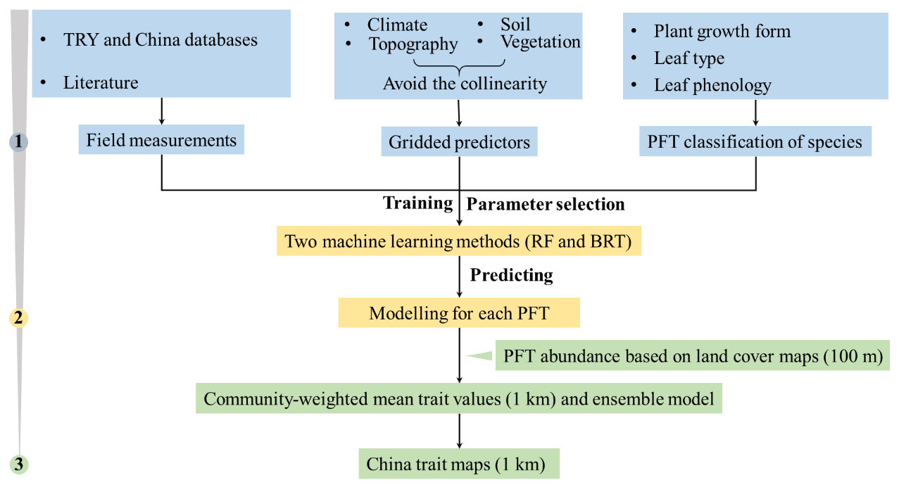
Figure 1 Methodological workflow for spatial mapping of plant functional traits. Trait mapping is performed in three steps. Step 1: in situ field measurements of plant functional traits, PFT classification of plant species and gridded predictors were collected. Step 2: two machine learning methods were used to predict trait values by training field measurements and predictors for each PFT. Step 3: spatialization of trait maps by calculating the abundance of each PFT using a 100 m land cover map and predicted trait values within a 1 km grid cell.

2.2 Plant functional trait collection and data processing

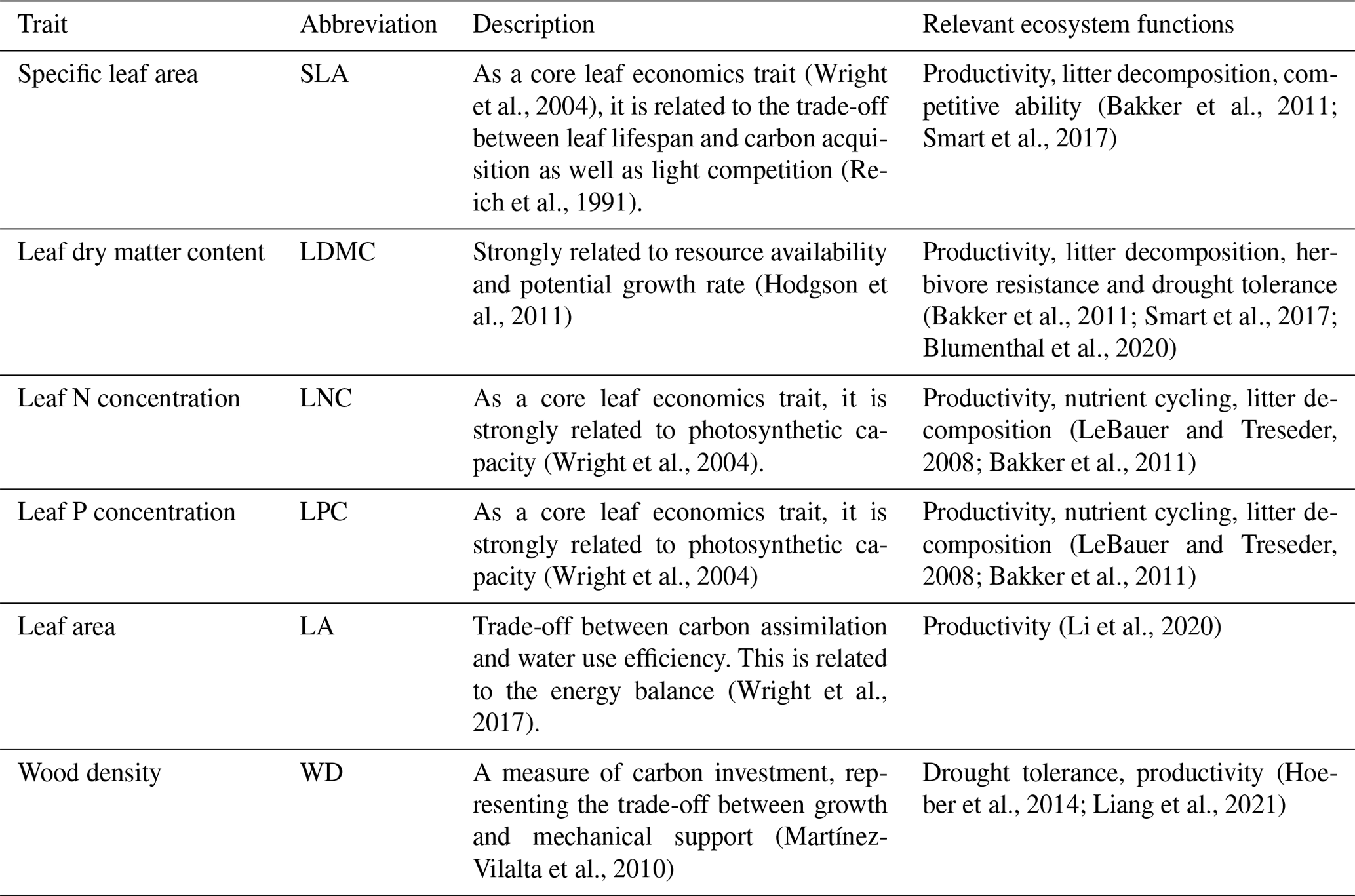
The information on the six plant functional traits and their ecological meanings are shown in Table 1. Plant trait data were obtained and collected via two main sources. The first source was public trait databases, including the TRY database (Kattge et al., 2020) and the China Plant Trait Database (Wang et al., 2018). The second source was from the literature (listed in the Supplement). To ensure data quality and comparability, we only included trait observations that met the following five criteria. (1) Measurements must be obtained from natural terrestrial fields in order to minimize the influence of management disturbance, and observations from croplands, aquatic habitats, control experiments and gardens were excluded. (2) According to the mass ratio hypothesis, the effect of plant species on ecosystem functioning is determined to an overwhelming extent by the traits and functional diversity of the dominant species and is relatively insensitive to the richness of subordinate species (Grime, 1998). Thus, we only included studies that measured plant trait observations from all the species or dominant species within a community. (3) In order to consider the intraspecific trait variation, when the same species occurred at the same sampling site from different studies, we included all the original observed data from different studies rather than averaging the values at the species level (Jung et al., 2010; Siefert et al., 2015). (4) Plant trait observations must be made on mature and healthy plant individuals, so some specific growth stages (e.g., seedling) and size classes (e.g., sapling) were excluded to reduce the confounding effect of ontogeny (Thomas, 2010). (5) We only included studies with clear geographical coordinates to match predictor variables. The sampling location and sampling time were also included in the dataset. The sampling time mostly focused on the growing season of a year (i.e., May–October), which can ensure the relative consistency of the sampling time to minimize the effects of seasonality. Plant functional traits must be sampled and measured according to standardized measurement procedures (Perez-Harguindeguy et al., 2013) to reduce the variation and uncertainty among different data sources. In this study, we included SLA measurements on sun leaves and WD measurements on the main stems of woody species.

Table 1 Description of the plant functional traits selected in this study and their relevant ecosystem functions.

The plant trait data were checked for possible errors and corrected in three steps as follows. First, species name and taxonomic nomenclature were corrected and standardized according to the Plant List (http://www.theplantlist.org/, last access: 10 March 2021) using the plantlist package. Second, illogical values, repeated values and outliers were removed, which were defined by observations exceeding 1.5 standard deviations from the mean trait value for a given species (Kattge et al., 2011). Third, we appended information on plant growth form, leaf type and leaf phenology from the TRY categorical traits database (https://www.try-db.org/TryWeb/Data.php#3, last access: 10 March 2021) and Flora Reipublicae Popularis Sinicae (http://www.iplant.cn/frps, last access: 10 May 2021), which were used to match species names to PFTs. We associated each species with a corresponding PFT based on plant growth form (tree, shrub and grass), leaf type (broadleaf and needleleaf) and leaf phenology (evergreen and deciduous). For example, the information on Salix matsudana is tree, deciduous and broadleaf, and thus we were able to associate the PFT of deciduous broadleaf forest (DBF) with this species. The species that did not correspond to any PFT were discarded. After these treatments, we collected a total of 34 589 trait measurements from 1430 sampling sites for our database, representing 3447 species from 195 families and 1066 genera (Fig. 2). Information on the statistics for the six plant functional traits collected in this study is shown in Table A1 in Appendix A.

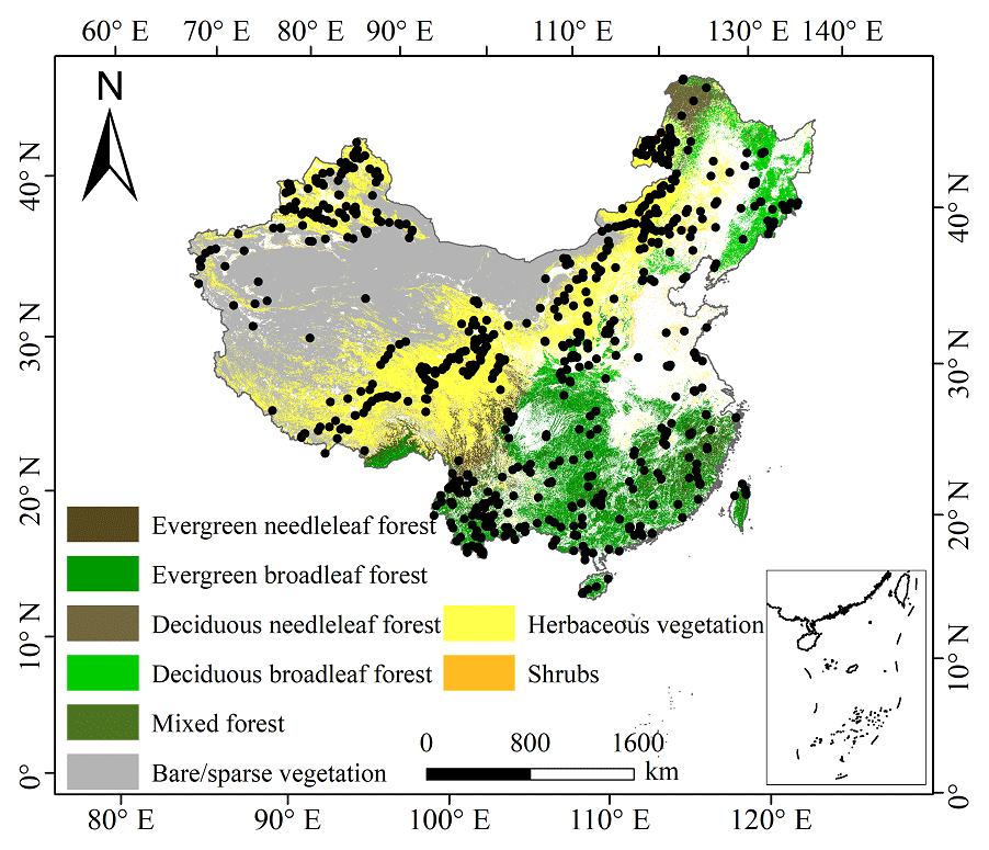
Figure 2 The spatial distribution of sample sites across different ecosystems in China. The white areas represent artificial land cover types.

2.3 Preparing predictor variables

2.3.1 Climate data

Twenty-one climate variables were used in this study, including 19 bioclimate variables, solar radiation (RAD) and aridity index (AI) (Table A2 in Appendix A). The 19 bioclimate variables and RAD were obtained from WorldClim version 2.1 for the period from 1970 to 2000 (https://www.worldclim.org/data/worldclim21.html, last access: 16 March 2021). The AI data were extracted from the CGIAR Consortium of Spatial Information (CGIAR-CSI) for the period from 1970 to 2000 (http://www.csi.cgiar.org, last access: 18 March 2021) (Trabucco and Zomer, 2018). The spatial resolution of the climate data is 1 km.

2.3.2 Soil data

Twelve soil variables were included in this study, representing different aspects of soil properties, i.e., soil texture, bulk density (BD), pH and soil nutrients (Table A2 in Appendix A). All the soil variables were extracted from the Soil Database of China for Land Surface Modeling (http://globalchange.bnu.edu.cn/research/soil2, last access: 13 June 2021) (Shangguan et al., 2013). Given the importance of topsoil properties for community composition (Bohner, 2005), we averaged the first four layers to represent the topsoil properties (∼30 cm) in our study. The spatial resolution is 1 km.

2.3.3 Topography

The topographic variable was elevation. Elevation data were extracted from the STRM 90m dataset in China based on the SRTM V4.1 database (https://www.resdc.cn/data.aspx?DATAID=123, last access: 13 April 2021). The spatial resolution is 1 km.

Given the collinearity among climate and soil variables, we reduced the dimensionality of these predictors based on Pearson's correlation coefficient (r) (Figs. A1 and A2 in Appendix A). Among a set of highly correlated variables (r>0.75), only one variable was retained in subsequent analysis to ensure a combination of different environmental variables. The final selection of environment predictors included 20 variables: mean annual temperature (MAT), mean diurnal range (MDR), minimum temperature of the coldest quarter (T_min), maximum temperature of the warmest quarter (T_max), temperature seasonality (TS), mean annual precipitation (MAP), precipitation seasonality (PS), precipitation of the wettest quarter (PEQ), precipitation of the driest quarter (PDQ), AI, RAD, elevation, soil sand content (SAND), pH, BD, soil total N (STN), soil total P (STP), soil available P (SAP), soil alkali-hydrolyzable N (SAN) and cation exchange capacity (CEC).

2.3.4 Vegetation indices

Three categories of vegetation indices were included in this study (Table A2 in Appendix A). First, the EVI was extracted from the MOD13A3 V006 product (https://lpdaac.usgs.gov/products/mod13a3v006/, last access: 28 May 2021). This product is available as a monthly average with a spatial resolution of 1 km, ranging from January 2000 to December 2018. Second, MODIS reflectance data were also extracted from the MOD13A3 V006 product, including MIR reflectance, NIR reflectance, red reflectance and blue reflectance. Third, the MERIS terrestrial chlorophyll index (MTCI) was extracted from the Natural Environment Research Council Earth Observation Data Centre (NEODC, 2005) (https://data.ceda.ac.uk/, last access: 28 May 2021). MTCI data are available globally as a monthly average at 4.63 km spatial resolution and range from June 2002 to December 2011. It is noted that valid MTCI values should be greater than 1, so our study deleted any values less than 1.

To avoid collinearity, we also reduced the dimensionality of vegetation indices based on r values (Fig. A3 in Appendix A). Most selected variables were related to the growing season due to plant functional traits being measured during the growing season. Furthermore, based on the results of Pearson's correlation analysis, the MTCI, MIR, NIR, red and blue in January showed low correlations with those in the growing season, and thus they were included in the subsequent analysis. The final selection included 36 variables: the annual EVI and monthly EVI (May, June, July, August and September) together with the monthly MTCI, MIR, NIR, red and blue (all for January, June, July, August and September).

Both environmental variables and vegetation indices were resampled to a consistent spatial resolution of 1 km using the nearest-neighborhood method.

PFT is also an important factor in influencing the variation of plant functional traits (Verheijen et al., 2016; Loozen et al., 2020), and thus the trait predictions were performed for each PFT individually. We used the 2015 land cover map at 100 m spatial resolution to calculate the relative abundance of each PFT within a 1 km grid cell, which was extracted from the Copernicus Global Land Service (CGLS-LC100, Version 3) (https://land.copernicus.eu/global/products/lc, last access: 24 May 2021) (Buchhorn et al., 2020). We focused on natural terrestrial vegetation, so all artificial land cover types (e.g., croplands) were eliminated in our dataset. Seven categories were included: evergreen needleleaf forest (ENF), evergreen broadleaf forest (EBF), deciduous needleleaf forest (DNF), deciduous broadleaf forest (DBF), shrubland (SHL), grassland (GRL) and bare or sparse vegetation.

2.4 Model fitting and validation

To predict the spatial patterns of plant functional traits, we used two machine learning models, i.e., random forest and boosted regression trees.

Random forest is an ensemble machine learning method based on classification and regression trees using collections of regression trees to classify observations according to a set of predictive variables (Breiman, 2001). This method repeatedly constructs a set of trees from random samples of training data, and the final prediction is produced by integrating the results of all individual trees, which makes it a robust method. The model is controlled by two main parameters: the number of sampled variables (mtry) and the number of trees (ntree). The mtry was set to range from 1 to 57 (at an interval of 1), and the ntree was set to 500, 1000, 2000, 5000 and 10 000 in subsequent runs. This analysis was performed using the randomForest function in the randomForest package (Liaw and Wiener, 2002).

Boosted regression trees are machine learning methods based on generalized boosted regression models using a boosting algorithm to combine many sample tree models to optimize predictive performance (Elith et al., 2006). There is no need for prior data transformation or the elimination of outliers, and this method can fit complex nonlinear relationships while automatically handling interaction effects between predictors (Elith et al., 2008). The four parameters to optimize in these models are the number of trees, interaction depth, learning rate and bag fractions. We varied the parameter settings to find the optimal parameter combination that achieves minimum predictive error. The number of trees was set to 3000; the interaction depth varied from 1 to 7 (at an interval of 1); the learning rate was set to 0.001, 0.01, 0.05 and 0.1; and the bag fraction was set to 0.5, 0.6, 0.7 and 0.75. PFT was used as a dummy variable in the boosted regression tree models. This analysis was conducted using the gbm function in the gbm package (Ridgeway, 2006).

We built a separate predictive model for each plant functional trait. To select the optimal parameter combination and to evaluate the final model performance for each trait, we calibrated the models 10 times using a randomly selected 80 % of the data for training models and validating against the remaining 20 % based on cross-validation (Table A3 in Appendix A). The predictive performance was evaluated by regressing the predicted and observed trait values from all repetitions of the cross-validation. The fitting performance of the random forest and boosted regression trees was evaluated using a determinate coefficient (R²), a normalized root-mean-square error (NRMSE) and a mean absolute error (MAE). These scores are calculated following Eqs. (1), (2) and (3):

$$\begin{array}{}\text{(1)}& {\displaystyle }{R}^{\mathrm{2}}=\mathrm{1}-{\displaystyle \frac{\sum _{i=\mathrm{1}}^n(p_i-o_i{)}^{\mathrm{2}}}{\sum _{i=\mathrm{1}}^n(p_{i-}\widehat{o_i}{)}^{\mathrm{2}}}},\text{(2)}& {\displaystyle }\mathrm{NRMSE}={\displaystyle \frac{\sqrt{\frac{\mathrm{1}}{n}\sum _{i=\mathrm{1}}^n(p_i-o_i{)}^{\mathrm{2}}}}{p_{\max }-p_{\min }}},\text{(3)}& {\displaystyle }\text{MAE}={\displaystyle \frac{\mathrm{1}}{n}}\sum _{i=\mathrm{1}}^n\mathrm{|}{o}_i-p_i\mathrm{|},\end{array}$$

where p_i and o_i are the predictive values and observed values, respectively; $\widehat{o_i}$ is the mean of the observed values.

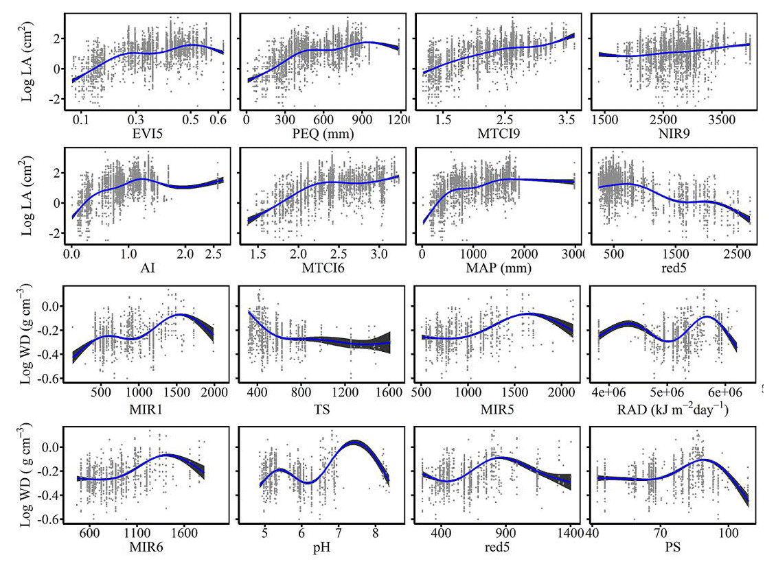
To quantify the relative importance of each predictor across the two models consistently, we used the method proposed by Thuiller et al. (2009). This method applies correlation between the standard predictions fitted with the original data and predictions where the variable under investigation has been randomly permutated. If the correlation is high, which indicates little difference between the two predictions, the variable permutated is considered unimportant for the model. This step was repeated multiple times for each predictor, and the mean correlation coefficient over runs was recorded. Then the relative importance of each predictor was quantified as 1 minus the Spearman rank correlation coefficient (see Boonman et al., 2020). In addition, we used generalized additive models to fit the relationships between plant functional traits and the most important variables using the gam function in the mgcv package.

2.5 Generation of plant functional trait maps and model performance

The generation of spatial maps of plant functional traits was performed in three steps. First, we predicted trait values separately for each natural PFT (i.e., EBF, ENF, DBF, DNF, SHL and GRL) within a 1 km grid cell. Second, the abundance of individual natural PFTs within a 1 km grid cell was estimated using a land cover map with a spatial resolution of 100 m. Third, refer to Eq. (4), which has been widely applied in the community (Garnier et al., 2004), and the final trait value in a given 1 km grid cell is calculated as the sum of the predicted trait values multiplied by the corresponding abundance of each natural PFT.

$$\begin{array}{}\text{(4)}& \mathrm{CWM}={\sum }_{i=\mathrm{1}}^n{W}_i{X}_i\end{array}$$

n is the total number of PFTs in a given grid, W_i is the relative abundance of the ith natural PFT, and X_i is the predicted trait value of the ith natural PFT.

To reduce the variability of different single models and to construct a more stable and accurate model, the ensemble model was further applied to merge the predictions of random forest and boosted regression trees according to their cross-validated R² values. The predicted value of the ensemble model was calculated in a given grid cell as described by Eq. (5) (Marmion et al., 2009). The model accuracy was calculated by regressing the predicted values of the ensemble model against the observed trait values.

$$\begin{array}{}\text{(5)}& \mathrm{Pred}\mathrm{\_}{\mathrm{EM}}_t={\displaystyle \frac{{\sum }_{m=\mathrm{1}}^{\mathrm{2}}({\text{pred}}_{m,t}\times r_{m,t}^{\mathrm{2}})}{{\sum }_{m=\mathrm{1}}^{\mathrm{2}}{r}_{m,t}^{\mathrm{2}}}}\end{array}$$

Pred_EM_t is the predicted value of the t trait in the ensemble model. pred_m,t is the predicted value of the t trait in the m model. $r_{m,t}^{\mathrm{2}}$ is the cross-validated R² of the t trait in the m model.

To evaluate the model performance (i.e., the variability in the prediction across the models), the coefficient of variation (CV) was calculated as the difference between the predictions of random forest and boosted regression tree methods and the ensemble model. The CV is calculated following Eq. (6):

$$\begin{array}{}\text{(6)}& {\text{CV}}_t={\displaystyle \frac{\frac{\sqrt{{\sum }_{m=\mathrm{1}}^{\mathrm{2}}({\text{pred}}_{m,t}-{\text{obs}}_t{)}^{\mathrm{2}}\cdot r_{m,t}^{\mathrm{2}}}}{{\sum }_{m=\mathrm{1}}^{\mathrm{2}}{r}_{m,t}^{\mathrm{2}}}}{{\text{obs}}_t}},\end{array}$$

where pred_m,t is the predicted value of the t trait in the m model, obs_t is the value of the t trait in the ensemble model, and $r_{m,t}^{\mathrm{2}}$ is the cross-validated R² of the t trait in the m model.

2.6 Uncertainty assessments

Multivariate environmental similarity surface analysis (MESS) was used to identify the range of extrapolated predictor values across the locations in the plant trait dataset (Elith et al., 2010). This method is often used to evaluate the extent of the extrapolation and the applicability domain. If the value is negative, this indicates that, at a given grid cell, at least one predictor variable is outside the extent of the referenced predictor layer. This analysis was conducted using the mess function in the dismo package.

All analyses were performed in R 4.0.2 (R Core Team, 2020).

3 Results

3.1 Performance of the prediction models

Cross-validation showed that the performance of the predictive models differed greatly among the plant functional traits (Tables 2, B1 and B2). WD had the best performance in all three models, with R² values of 0.64, 0.68 and 0.67 for the random forest, boosted regression trees and ensemble model, respectively. SLA and LPC had R² values greater than 0.45, while LDMC performed the worst, with R² values below 0.30.

Table 2 Results of plant functional traits for cross-validated R², NRMSE and MAE for random forest, boosted regression trees and the ensemble model.

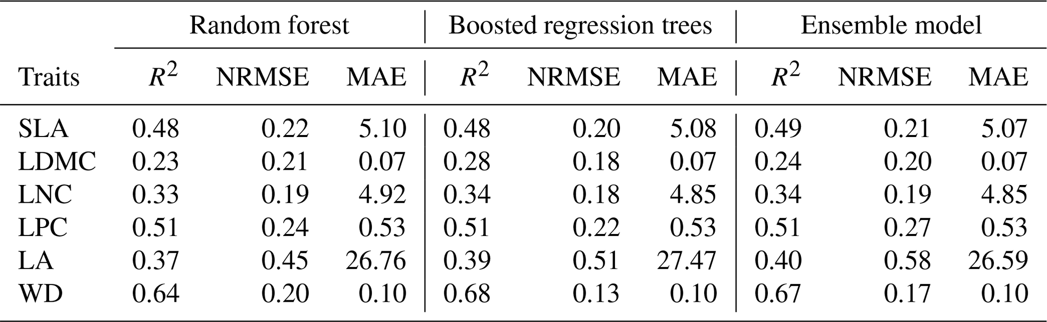
SLA: specific leaf area (m² kg⁻¹); LDMC: leaf dry matter content (g g⁻¹); LNC: leaf N concentration (mg g⁻¹); LPC: leaf P concentration (mg g⁻¹); LA: leaf area (cm²); WD: wood density (g cm⁻³); R²: determinate coefficient; NRMSE: normalized root-mean-square error; MAE: mean absolute error.

3.2 Spatial patterns of predicted plant functional traits

There were relatively consistent spatial patterns for SLA, LNC and LPC, with high values in northeastern and northwestern China and the southeastern Qinghai–Tibetan Plateau, together with low values in southwestern China (Figs. 3a, c, d, C1, C2, C3, C5 and C6). SLA and LPC increased with latitude, while LNC did not vary significantly along the latitudinal gradient. For SLA, LNC and LPC, the variability was low among random forest, boosted regression trees and ensemble model, with an overall CV of less than 0.30 (Fig. 4a, c and d). LDMC values were relatively high in most regions of China, and the low values were mainly located in eastern Yunnan Province and the Loess Plateau (Figs. 3b, C1, C2 and C4). LA showed high values in the northeastern and southern regions (except for the Sichuan Basin) and the southeastern Qinghai–Tibetan Plateau (Figs. 3e, C1, C2 and C7). The strong latitudinal gradient was observed in LA, where the values decreased with latitude.

The CV values of LPC decreased with latitude, but other traits did not show latitudinal patterns (Fig. 4). The CV values of LA were relatively high, especially in northwestern China and the Inner Mongolia–Loess Plateau region (Fig. 4e). WD had high values in the northeastern and southern regions (Figs. 2f, C1, C2 and C8), while the CV values for WD were low throughout China (Fig. 4f).

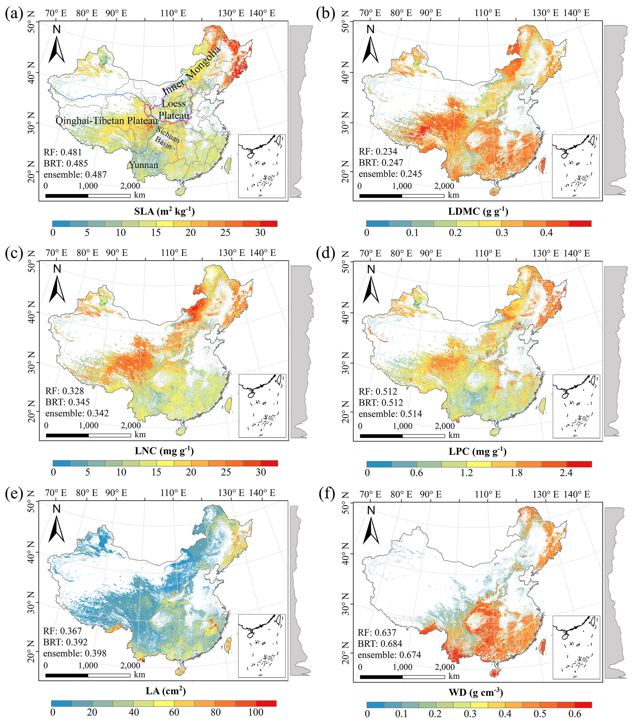
Figure 3 Spatial patterns of predicted plant functional traits in China based on the ensemble model. The grey curves to the right of the maps display the trait distribution along with the latitude. The white areas represent artificial land cover types and bare vegetation. The lines in grey, blue and purple represent the boundaries of the provinces, the Qinghai–Tibetan Plateau and the Loess Plateau, respectively. RF: random forest; BRT: boosted regression trees; ensemble: ensemble model; SLA: specific leaf area; LDMC: leaf dry matter content; LNC: leaf N concentration; LPC: leaf P concentration; LA: leaf area; WD: wood density.

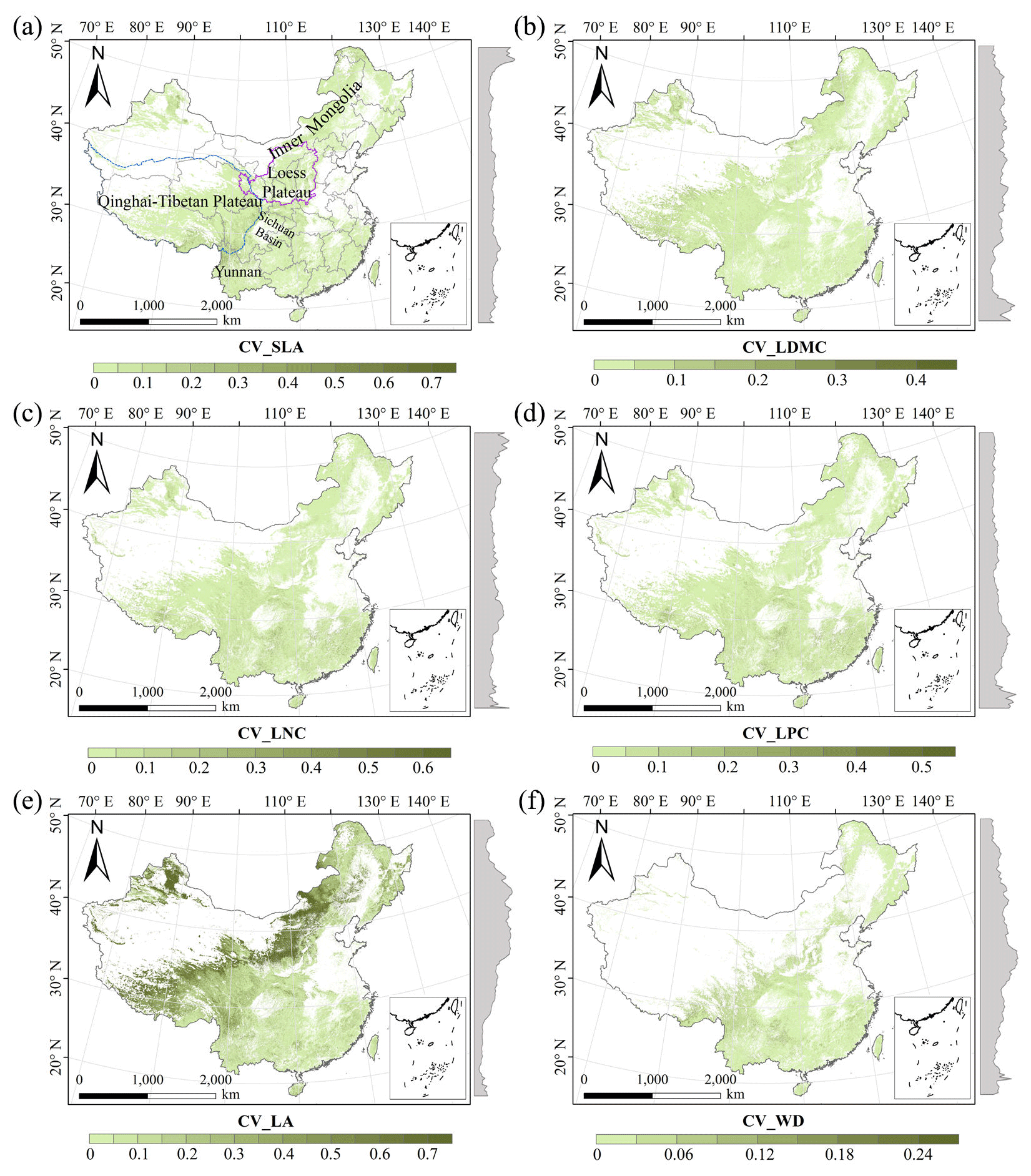
Figure 4 The variability in plant functional trait predictions among the random forest, boosted regression trees and ensemble model. The grey curves to the right of the maps display the coefficient of variation along with the latitude. The white areas represent artificial land cover types and bare vegetation. The lines in grey, blue and purple represent the boundaries of the provinces, the Qinghai–Tibetan Plateau and the Loess Plateau, respectively.

3.3 Relative importance of predictive variables

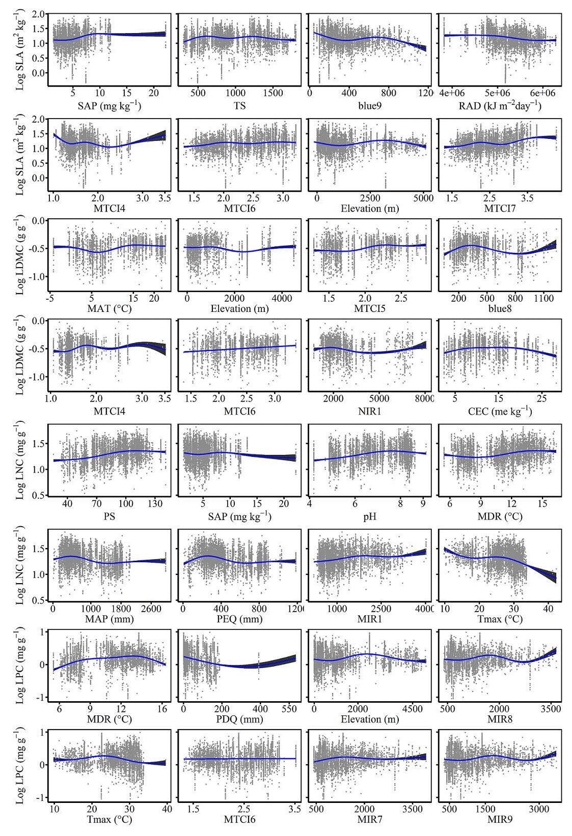
The dominant factors explaining spatial variation differed greatly among plant functional traits (Table 3). Overall, climate variables were more important for predicting plant functional traits than were soil variables. Temperature variables (i.e., MAT, MDR and TS) showed close relationships with SLA, LDMC, LPC and WD, while precipitation variables (i.e., PS, PEQ, MAP and PDQ) were more important for predicting the spatial patterns of LNC, LPC and LA. RAD was the fourth most dominant factor in predicting the spatial patterns of SLA and WD. Elevation also played an important role in LDMC and LPC predictions. Within soil variables, soil nutrients (i.e., pH and SAP) showed close associations with SLA and LNC. In addition to the environmental variables, MTCI emerged as an important predictor for explaining SLA, LDMC and LA. Finally, the EVI was the most important predictor for LA, and MIR values in January and May were the primary predictors of WD. The relationships between plant functional traits and the most important variables are shown in Figs. D1 and D2 in Appendix D.

Table 3 List of the eight most important variables for plant functional trait predictions.

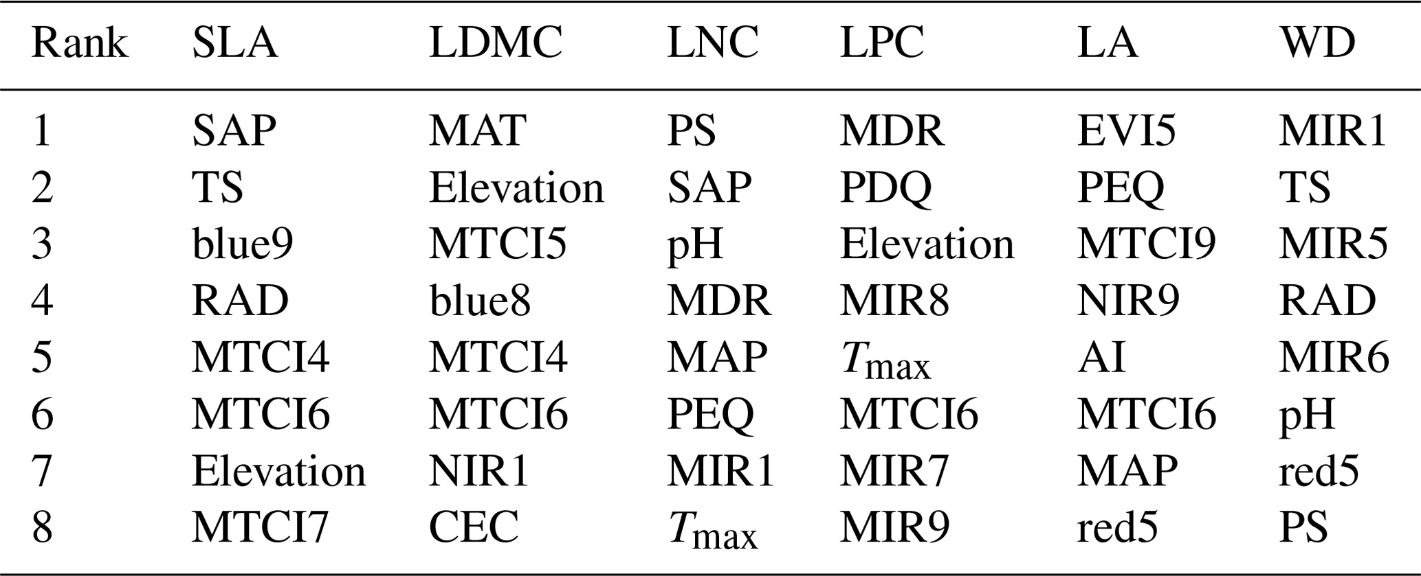
SLA: specific leaf area (m² kg⁻¹); LDMC: leaf dry matter content (g g⁻¹); LNC: leaf N concentration (mg g⁻¹); LPC: leaf P concentration (mg g⁻¹); LA: leaf area (cm²); WD: wood density (g cm⁻³); SAP: soil available P; TS: temperature seasonality; blue: blue reflectance; RAD: solar radiation; MTCI: MERIS terrestrial chlorophyll index; MAT: mean annual temperature; NIR: near-infrared reflectance; CEC: cation exchange capacity; PS: precipitation seasonality; MDR: mean diurnal range; MAP: mean annual precipitation; PEQ: precipitation of the wettest quarter of a year; MIR: middle infrared reflectance; T_max: maximum temperature of the warmest month of a year; PDQ: precipitation of the driest quarter of a year; EVI: enhanced vegetation index; AI: aridity index; red: red reflectance.

3.4 Model performance

The distributions of the predicted values based on random forest, boosted regression trees and ensemble model were consistent with the original observations, especially the peak values (Fig. 5). The mean values of the trait observations were relatively higher than those of the predicted values.

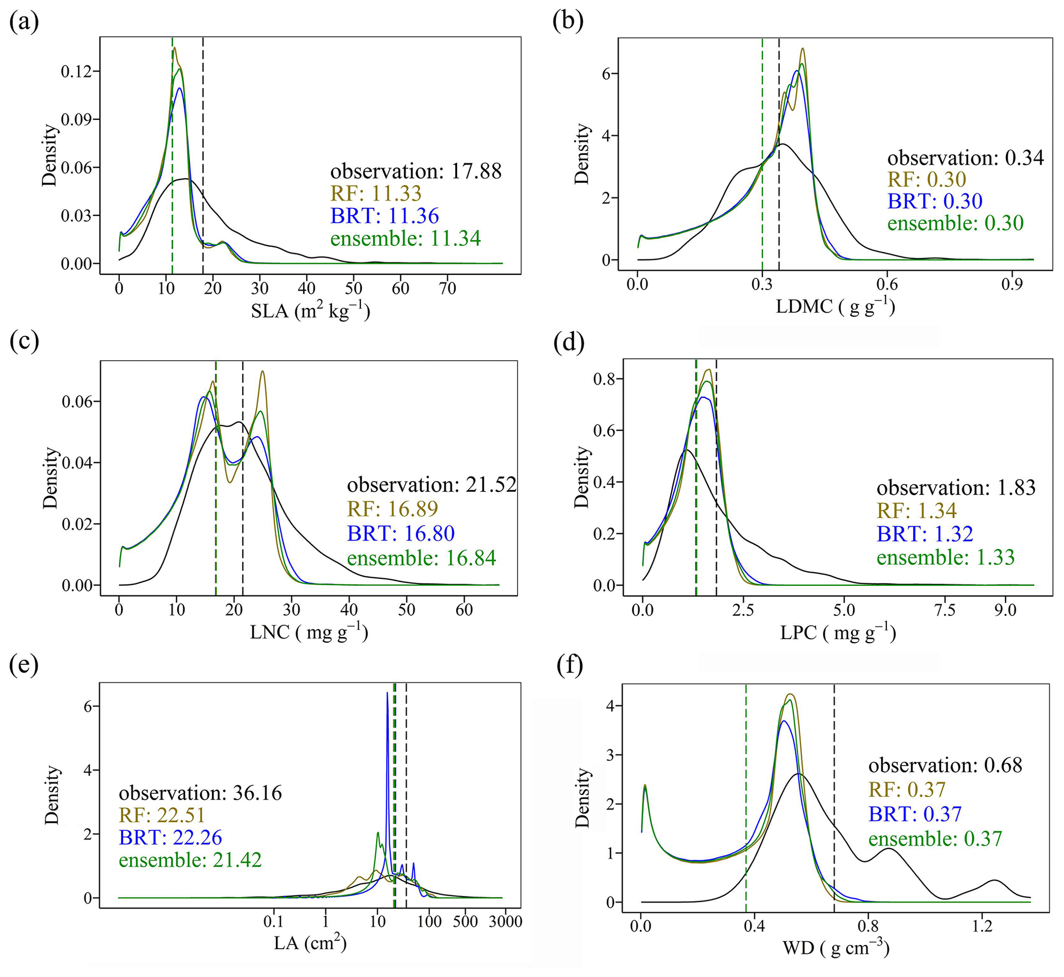
Figure 5 Comparison of trait distribution between observations and predictions in the three models. Each panel depicts the distribution of observations in solid black, of the RF in yellow, of the BRT in blue, and of the ensemble model in green. The dashed vertical lines indicate mean values.

3.5 Uncertainty assessments

The MESS values of all plant functional traits were positive in most regions, indicating a wide applicability domain of our models (Fig. 6). Nevertheless, trait predictions should be interpreted carefully for northeastern China and the Qinghai–Tibetan Plateau due to sparse samplings in these regions.

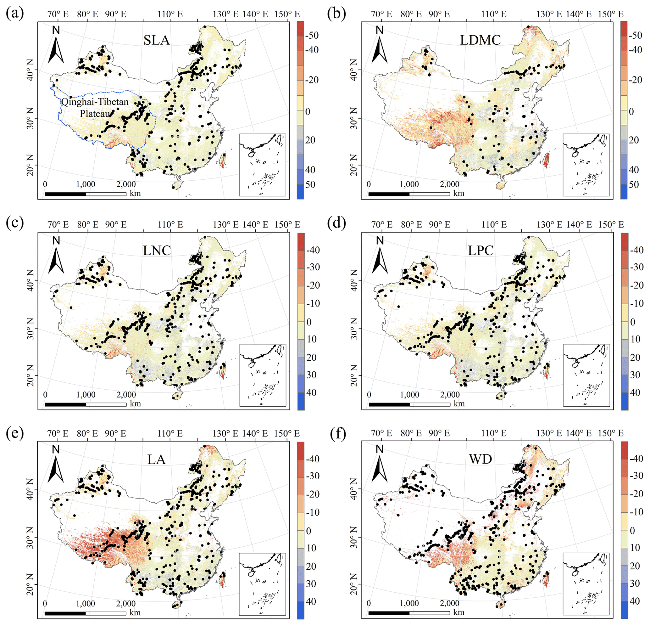
Figure 6 Multivariate environmental similarity surface (MESS) assessments for the six plant functional traits. The blue line represents the boundary of the Qinghai–Tibetan Plateau. The black dots represent the locations of the trait observations. More intense shades indicate a greater similarity (blue) or difference (red) in the environmental conditions of the location compared to the predictive factors covered by the training dataset. The white areas represent artificial land cover types and bare vegetation.

4 Discussion

4.1 Comparison with previous work

Our study predicted the spatial patterns of six key plant functional traits across China using machine learning methods and identified the applicability domain of the models. WD had the highest precision with an average of R² of 0.66, which was higher than the global WD prediction (Boonman et al., 2020). This improvement in precision may be attributed to the large number and dense occurrence of sample sites as well as the inclusion of vegetation indices in our study. In addition, SLA and LPC showed good accuracy with an R² value of 0.50, which was higher than that of Boonman et al. (2020) and consistent with that of Moreno-Martínez et al. (2018). However, LNC and LA showed relatively poor performance, which may be related to the reason that the two traits were more influenced by phylogeny than environmental variables (Yang et al., 2017; An et al., 2021). In addition, we found that mean values of trait predictions were lower than those of observations, which may be attributable to the reason that the mean values of trait observations were from the individual level, while the mean values of predicted values were based on the relative abundance of PFTs and the corresponding predicted values within a 1 km grid cell.

The frequency distributions of plant functional traits in China differed between our study and previous studies (Figs. 7 and E1, Table E1). Given that the spatial resolution of trait maps in most previous studies was 0.5° (except for Moreno-Martínez et al., 2018, and Vallicrosa et al., 2022), we resampled the data products of previous studies and our study to 0.5° spatial resolution. The distributions in our study contained more predictions at lower values of SLA, LNC and LPC and were broader than those for SLA and LNC in previous global studies. However, the distribution of LNC in our study was consistent with that in the study of Vallicrosa et al. (2022) with 1 km spatial resolution (Fig. E1 in Appendix E). LA in our study contained more predictions at higher values and was also broader than those in previous global studies. WD did not show lower and higher predicted values in this study. However, the WD values in the studies of Boonman et al. (2020) and Schiller et al. (2021) had more predictions at higher values and no lower values (<0.30 g cm⁻³). Our predicted values of SLA showed the highest spatial correlation with those of Dong et al. (2023), and LNC showed the strongest spatial correlation with those of Butler et al. (2017) (Table 4). LA and WD showed the best spatial correlation with those of Schiller et al. (2021), but LPC showed a relatively weak spatial correlation with those of published studies.

In addition, we compared our results with other studies focused on China. Yang et al. (2016) predicted the spatial distributions of leaf mass per area (i.e., 1 / SLA) and LNC based on trait–environment relationships in China and had R² values of 0.13–0.16. The lower predictive precision may be because Yang et al. (2016) only used MAT, MAP and RAD as predictors in estimating the spatial patterns of leaf mass per area and LNC, which likely led to poor performance and low heterogeneity. These results also demonstrated the advantage of our methods in mapping the spatial patterns of plant functional traits at a regional scale.

Table 4 Spatial correlations for SLA, LNC, LPC, LA and WD between this study and previous trait maps, labeled by the first author of the corresponding publication (see Table E1 in Appendix E for citations).

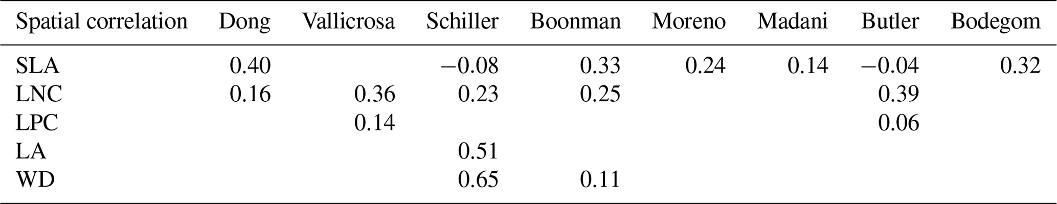
The spatial correlation of leaf dry matter content (LDMC) between our study and previous studies was not included, as the LDMC maps were not available. SLA: specific leaf area (m² kg⁻¹); LNC: leaf N concentration (mg g⁻¹); LPC: leaf P concentration (mg g⁻¹); LA: leaf area (cm²); WD: wood density (g cm⁻³).

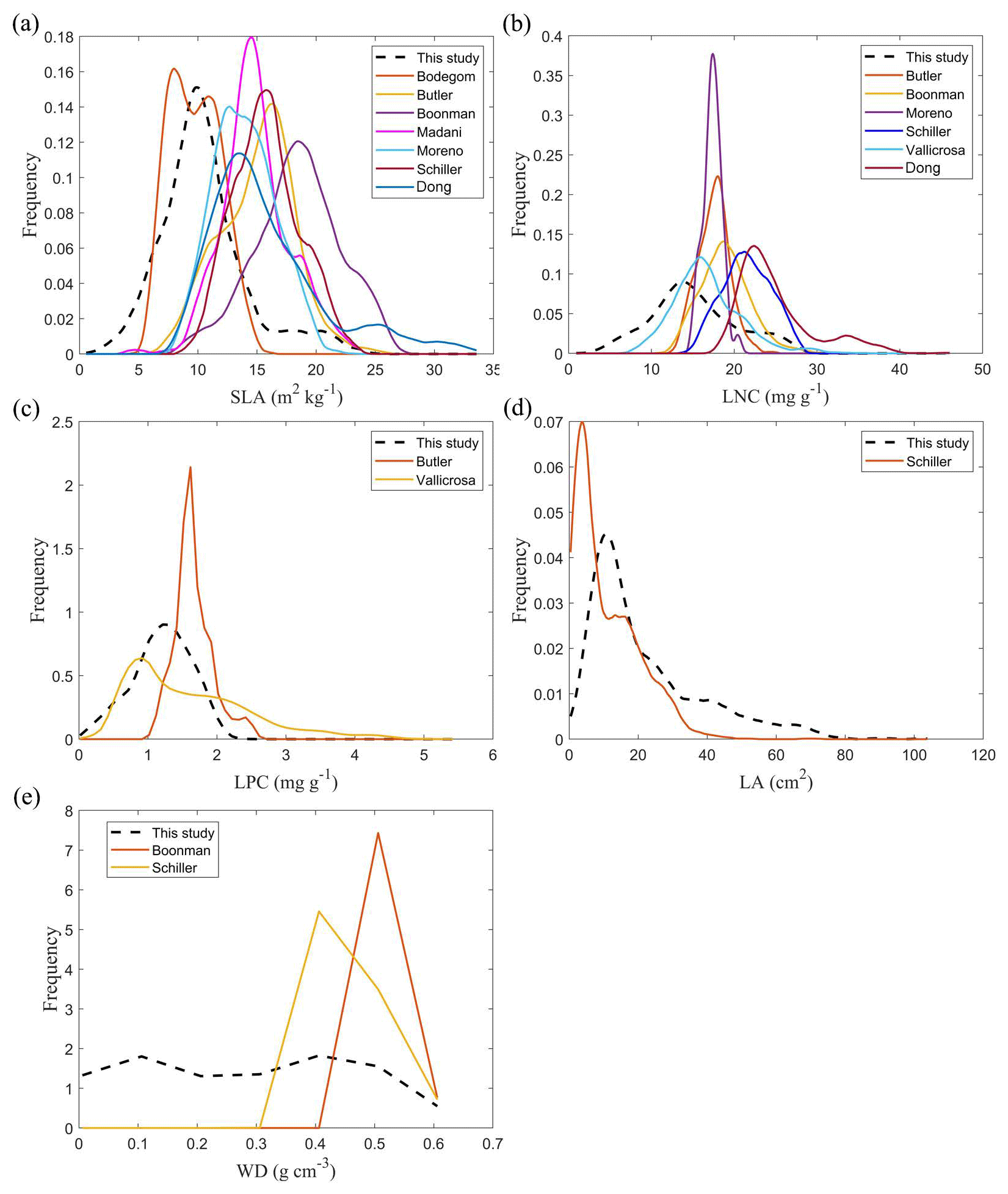
Figure 7 Frequency distributions of plant functional traits in our study (“This study”, dashed black lines) and other trait maps identified by the first author of the corresponding publication (see Table E1 for citations).

4.2 Spatial patterns of plant functional traits in China

Our study revealed the spatial patterns of different plant functional traits across China, and the variability among the two machine learning methods was relatively low. We compared the spatial differences of trait maps between our study and previous studies at the global scale (Figs. E2–E6 in Appendix E). For example, our study showed high SLA values in the southeastern Qinghai–Tibetan Plateau, which concurred with the global study of Boonman et al. (2020). The spatial difference of SLA between our study and van Bodegom et al. (2014) was relatively low, and the predicted values in most regions were slightly lower in our study than those in van Bodegom et al. (2014). The spatial pattern of the difference in SLA between our study and Moreno et al. (2018), Butler et al. (2017) and van Bodegom et al. (2014) was consistent, and the values were higher in northeastern China and the southwestern Qinghai–Tibetan Plateau in our study than those studies. Our study showed higher LNC values in northern Inner Mongolia, the Loess Plateau, the eastern Qinghai–Tibetan Plateau and northwestern China than those global studies (Butler et al., 2017; Moreno-Martínez et al., 2018; Boonman et al., 2020; Vallicrosa et al., 2022; Dong et al., 2023), reflecting the consistent spatial pattern among these studies. However, Yang et al. (2016) predicted high LNC values in northeastern and northwestern China, northern Inner Mongolia and the entire Qinghai–Tibetan Plateau, and SLA and LNC had low heterogeneity overall. The discrepancy with Yang et al. (2016) may be attributed to spatial extrapolation based on trait–climate relationships with a low predictive precision. There was no consistent spatial pattern in LPC between our study and previous studies. Consistent with the global pattern (Wright et al., 2017), LA was larger in the southern regions than in the northern regions and showed a decreasing trend with latitude. In addition, LA and WD values in our study were lower in most regions than those at the global scale. These discrepancies between our study and previous studies at the global scale may be related to three reasons. First, there is bias in the available in situ field measurement data from China in global studies, with a large gap in western China for SLA and no data in China for WD (Boonman et al., 2020). Second, some trait–environment relationships may be scale-dependent (Bruelheide et al., 2018), and these studies we compared are from the global scale because the trait maps in China are not available. Third, the methods used for trait mapping were different among studies, including eco-evolutionary optimality models (Dong et al., 2023), convolutional neural networks based on RGB photographs (Schiller et al., 2021), machine learning algorithms (Vallicrosa et al., 2022; Boonman et al., 2020) and multiple regression analysis (van Bodegom et al., 2014).

Moreover, our study also identified the applicability domain of our models for predicting the spatial patterns of plant functional traits across China. Five leaf traits and WD appeared to have poor applicability in northeastern China and the Qinghai–Tibetan Plateau, primarily due to sparse samplings. Future studies predicting plant functional traits across a large scale through remote sensing observations or other supplementary data will be needed to re-evaluate our results.

4.3 The role of predictive variables

Our study indicated that environmental variables were important for predicting the spatial patterns of plant functional traits, especially climate variables. Temperature variables were primary predictors for SLA, LDMC, LPC and WD. The relationships between leaf traits and temperature have been widely discussed in global and regional studies (Reich and Oleksyn, 2004; Bruelheide et al., 2018). The positive linkage between WD and temperature may be driven by changes in water viscosity. Plants can adapt to low water viscosity at high temperatures by reducing the diameter and density of their vessels and thickening cell walls (Roderick and Berry, 2002; Thomas et al., 2004). Precipitation variables were important predictors for leaf nutrient traits and LA. For example, precipitation of the wettest quarter of a year was the factor that most influenced LA variation, which has been confirmed by a previous study (An et al., 2021). A smaller LA could be an adaptive strategy to decrease water loss by reducing the surface area for transpiration under dry environmental conditions (Du et al., 2019). Although the effects of soil on trait predictions were relatively weak, we found that SAP and pH played key roles in SLA and LNC predictions. These results were similar to those of the previous studies reporting that soil pH was an important driver of trait variation at the global scale and in tundra regions (Maire et al., 2015; Kemppinen et al., 2021). Additionally, from the perspective of cost-efficient theory, the strong effects of SAP reflected the fact that high SLA may be an adaptation for facilitating soil exploration more efficiently in fertile soils (Freschet et al., 2010).

Vegetation indices were recently proposed as important predictors of spatial patterns of plant functional traits (Loozen et al., 2018). Our results corroborated these findings and further suggested that EVI, MTCI and MIR reflectances were important predictors in models. Here, the underlying mechanisms between vegetation indices and plant functional traits were not further discussed due to their complexity. However, our results indicated that vegetation indices and NIR reflectance were not key predictors of LNC estimation, which contrasted with the findings from global and regional studies (Wang et al., 2016; Loozen et al., 2018; Moreno-Martínez et al., 2018). This may be related to the multitude of factors that influence the relationships between LNC and vegetation indices and NIR reflectance, such as forest type and canopy structure (Dahlin et al., 2013).

4.4 Uncertainties

Although our study mapped the spatial patterns of key functional traits in terrestrial ecosystems across China through large-scale field investigations and compared the predictions with previous studies at global and regional scales, there persisted some uncertainties in the interpretation of these results. First, the predictive ability of models was relatively worse for certain traits, especially LDMC. Beyond the environmental effects, the variation in plant functional traits is also regulated by the phylogenetic structure among plant species (e.g., family, order or phylogenetic clade) (Li et al., 2017). Consequently, incorporating phylogenetic information will be a promising avenue for further improving the accuracy of spatial predictions of plant functional traits (Butler et al., 2017). A second potential issue is sampling bias; there are major spatial gaps in field investigations in northeastern China and the Qinghai–Tibetan Plateau. Due to the few measurements for shrubs and herbs, WD data are mainly confined to eastern forests, and the overall quantity of the WD data is much lower than that of leaf traits, even in the TRY database. The environmental information of the sampling sites was not always obtained from the original literature, and thus using the public environmental products is a common resolution in large-scale plant trait studies (Boonman et al., 2020; Vallicrosa et al., 2022). Such a mismatch between in situ trait measurements and predictors should be resolved in further work. Finally, an additional key challenge in data availability must be resolved to scale up from the species to community levels, in particular with data surrounding species co-occurrence and their relative cover or abundance in ecological communities (He et al., 2023). For example, global biodiversity data (e.g., the sPlot and Global Biodiversity Information Agency databases) that contain information on species occurrence or the proportion of species in a community have the potential to enable the calculation of community-weighted trait values and the re-evaluation of our results in future work (Telenius, 2011; Bruelheide et al., 2019). The lack of a consistent time period and spatial resolution of predictors due to limitation of data availability is a key challenge in the spatial mapping of plant functional traits. In addition, although the WorldClim version 2.1 product has high spatial resolution and includes various aspects of climatic parameters, there exist a certain limitation and uncertainty in predicting trait maps. Therefore, integrating satellite remote sensing monitoring methods with in situ trait data can also provide an effective way of estimating and assessing species diversity at large scales (Cavender-Bares et al., 2022).

4.5 Potential applications

Maps of these key functional traits in terrestrial ecosystems highlighted large-scale variability in space, which will significantly advance ecological analyses and future interdisciplinary research. First, using the spatially continuous trait maps, one can optimize and develop trait-flexible vegetation models to reduce the uncertainty of conventional vegetation models based on PFTs, which allows for exploration of the community assembly rules based on how plants with different trait combinations perform under a given set of environmental conditions (Berzaghi et al., 2020). When trait-flexible vegetation models are available, incorporating trait maps into models will bridge the gap for vegetation classifications and predictions of vegetation distribution under global change (van Bodegom et al., 2012; Yang et al., 2019). Second, most studies focused on the effects of plant functional traits on ecosystem carbon processes at individual, species and community scales, while how such effects scale up to regional or larger scales remains challenging. In addition, the assessments of China's terrestrial ecosystem carbon sink have large uncertainties (Piao et al., 2022). The spatial continuous trait maps will provide an effective way of linking ecosystem characteristics to ecosystem carbon sink estimates in China (Madani et al., 2018; Šímová et al., 2019). These analyses will help shed light on the mechanisms underlying plant functional traits and terrestrial ecosystem carbon storage at a large scale.

5 Data availability

The original plant functional trait data collected in this study that were used for machine learning models (named by the data file used for machine learning models.csv) and the final maps of plant functional traits in GeoTIFF format (named by the plant functional trait category) are available at https://doi.org/10.6084/m9.figshare.22351498 (An et al., 2023).

6 Conclusions

We generated a set of spatial continuous trait maps at 1 km spatial resolution using machine learning methods in combination with field measurements, environmental variables and vegetation indices. Models for leaf traits (except for LDMC) and WD showed good accuracy and robustness, whereas models of LDMC had relatively poor precision and robustness. Temperature variables were the most important predictors for leaf traits (except for LA) and WD, and precipitation variables were the most important predictors for leaf nutrient traits and LA. We caution that plant functional trait predictions should be interpreted carefully for northeastern China and the Qinghai–Tibetan Plateau. The spatial continuous trait maps generated in our study are complementary to current terrestrial in situ observations and offer new avenues for predicting large-scale changes in vegetation and ecosystem functions under climate scenarios in China.

Appendix A

Table A1 Summary of statistics in the plant functional traits, environmental variables and geographical distribution in China.

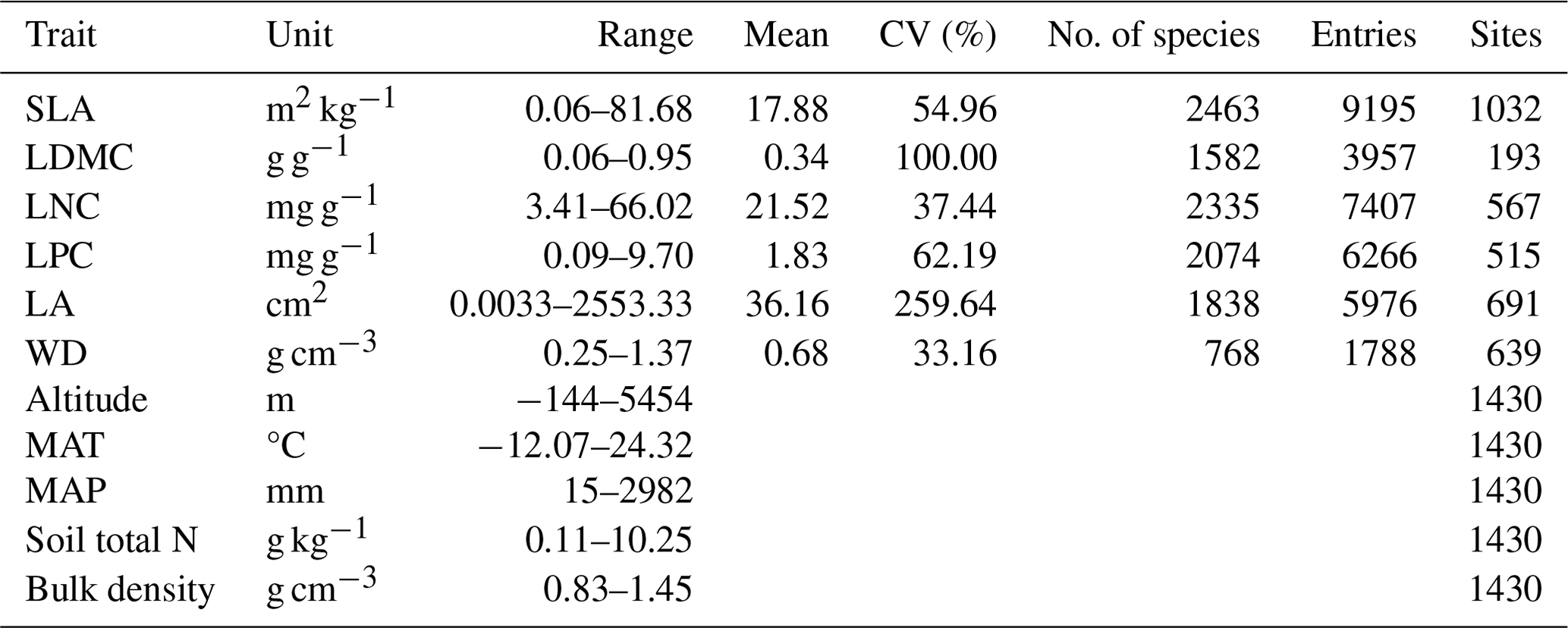
SLA: specific leaf area; LDMC: leaf dry matter content; LNC: leaf N concentration; LPC: leaf P concentration; LA: leaf area; WD: wood density; MAT: mean annual temperature; MAP: mean annual precipitation.

Table A2 List of all the predictors, including the environment and remote sensing variables used in this study.

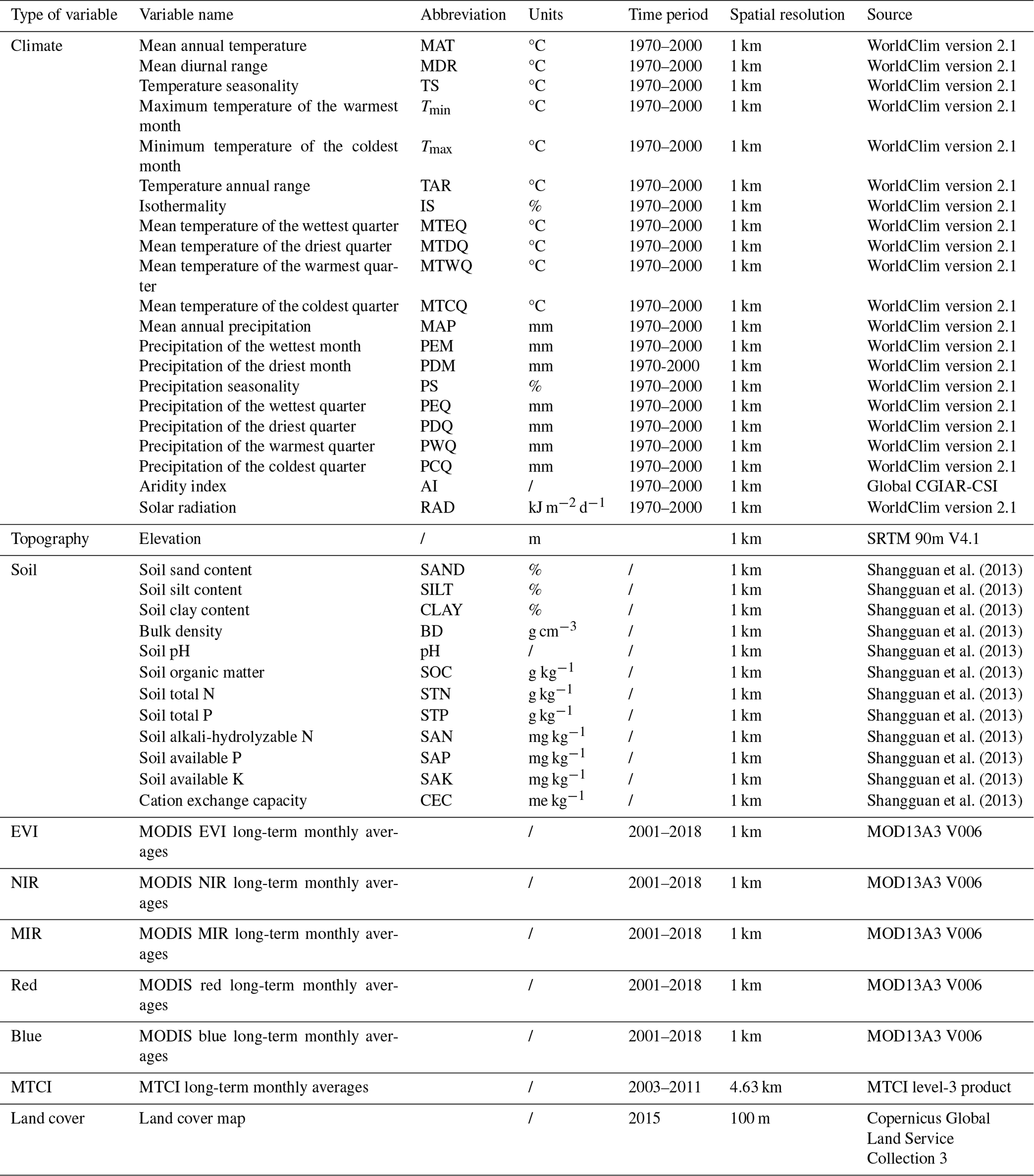
The vegetation indices are calculated as long-term monthly averages from 2001 to 2018. Thus, 12 variables of each vegetation index category are obtained.

Table A3 The number of samples of the six plant functional traits used for model training (80 %) and validation (20 %).

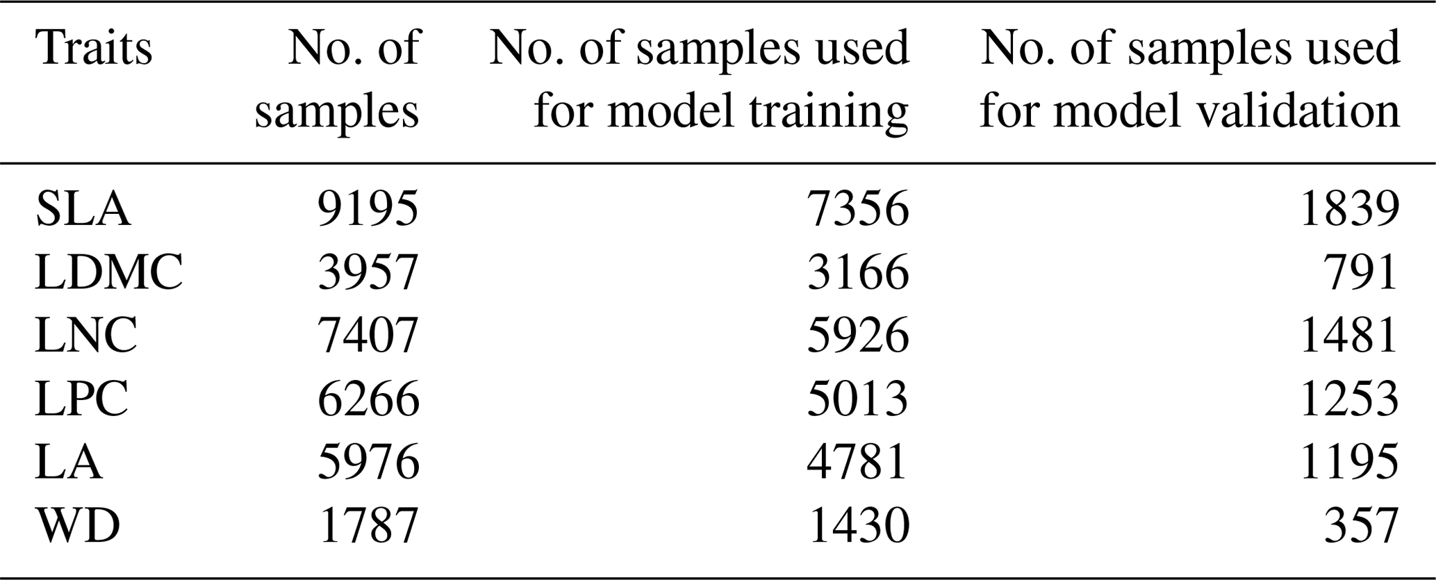
SLA: specific leaf area (m² kg⁻¹); LDMC: leaf dry matter content (g g⁻¹); LNC: leaf N concentration (mg g⁻¹); LPC: leaf P concentration (mg g⁻¹); LA: leaf area (cm²); WD: wood density (g cm⁻³).

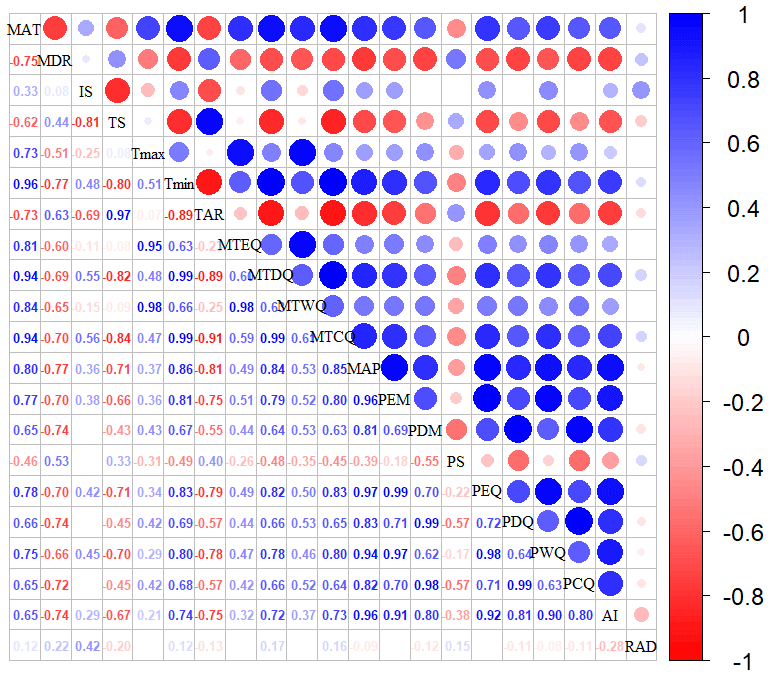
Figure A1 Correlations among climate variables. The blank indicates that the correlations are not significant (P>0.05). The size of the circles is proportional to the correlation coefficient. The abbreviations of the climate variables are seen in Table A2.

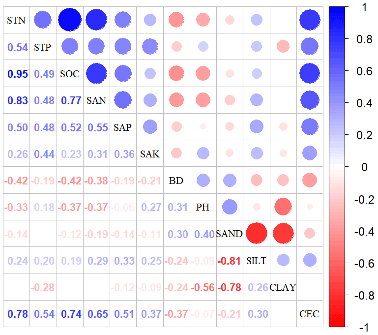
Figure A2 Correlations among soil variables. The blank indicates that the correlations are not significant (P>0.05). The size of the circles is proportional to the correlation coefficient. The abbreviations of the soil variables are seen in Table A2.

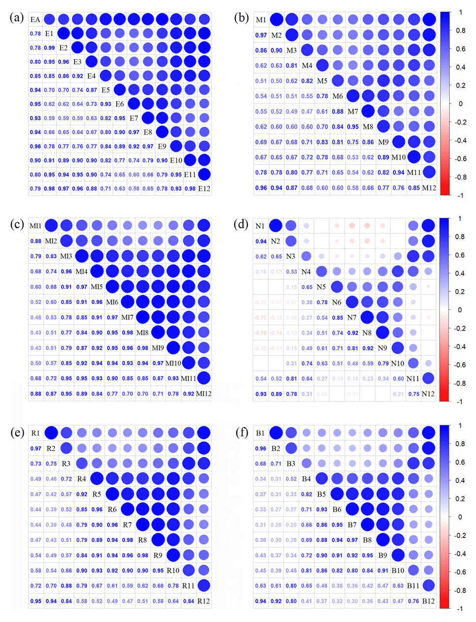
Figure A3 Correlations among monthly vegetation index variables. The blank indicates that the correlations are not significant (P>0.05). The size of the circles is proportional to the correlation coefficient. (a) Enhanced vegetation index (EVI); (b) MERIS terrestrial chlorophyll index (MTCI); (c) MIR reflectance; (d) NIR reflectance; (e) red reflectance; (f) blue reflectance.

Appendix B

Table B1 Optimal parameter combination and model performance of random forest for plant functional traits.

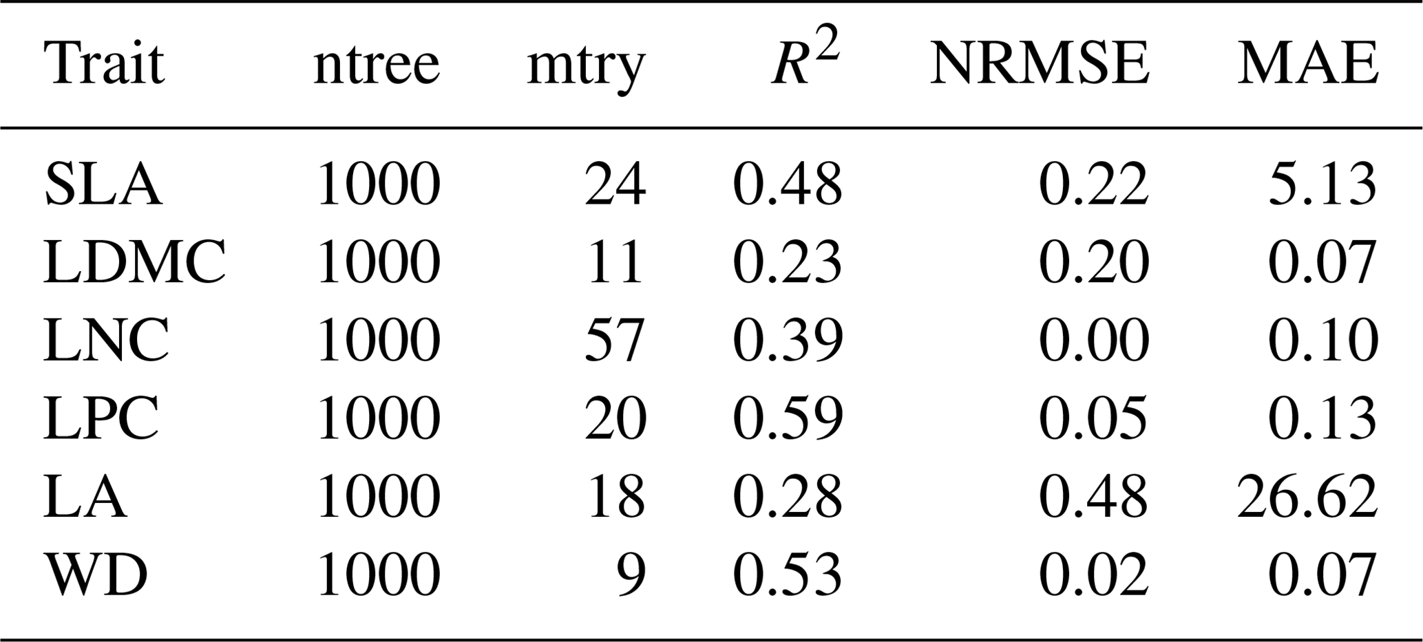
SLA: specific leaf area; LDMC: leaf dry matter content; LNC: leaf N concentration; LPC: leaf P concentration; LA: leaf area; WD: wood density; R²: determinate coefficient; NRMSE: normalized root-mean-square error; MAE: mean absolute error.

Table B2 Optimal parameter combination and model performance of boosted regression trees for plant functional traits.

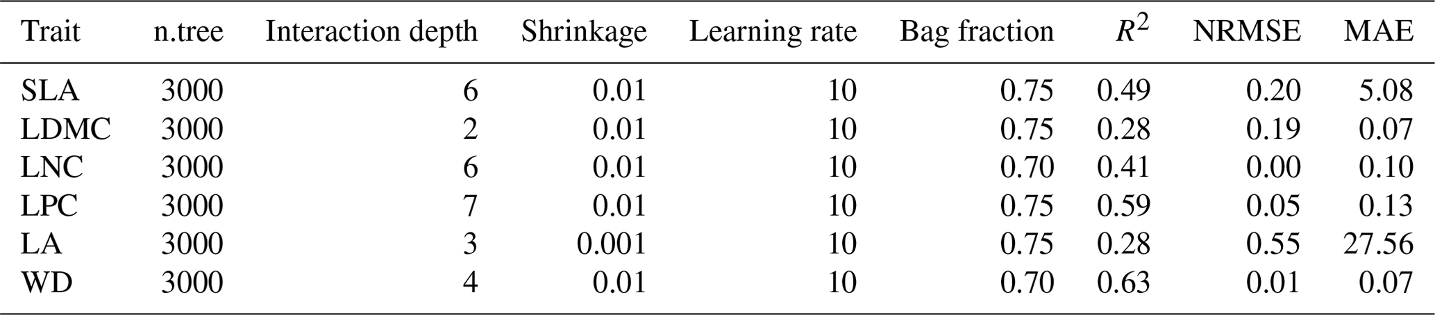
SLA: specific leaf area; LDMC: leaf dry matter content; LNC: leaf N concentration; LPC: leaf P concentration; LA: leaf area; WD: wood density; R²: determinate coefficient; NRMSE: normalized root-mean-square error; MAE: mean absolute error.

Appendix C

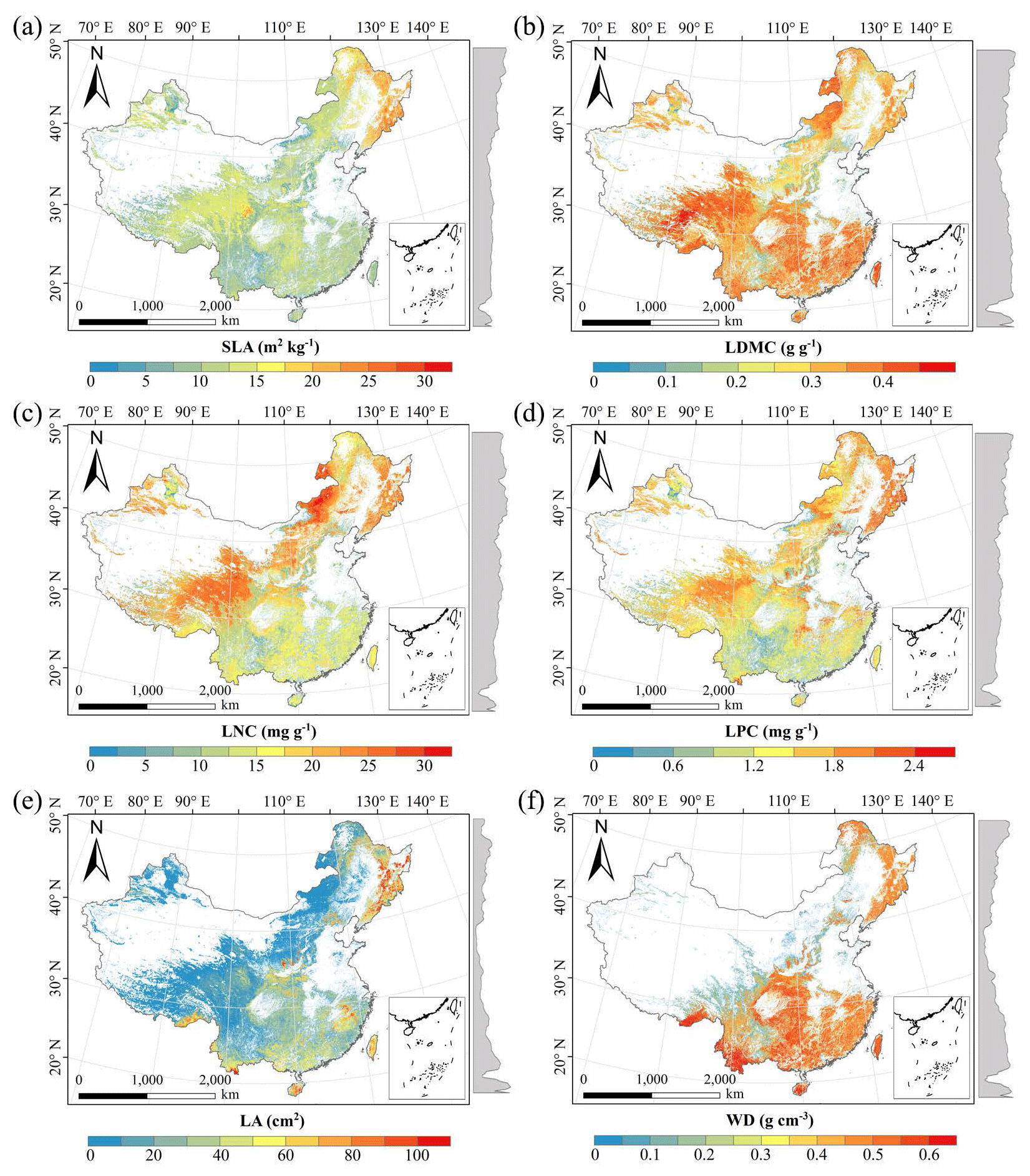
Figure C1 Spatial distributions of plant functional traits based on random forest. The grey curves on the right of the maps are the trait distribution along with the latitude. The white areas represent artificial land cover types and bare vegetation.

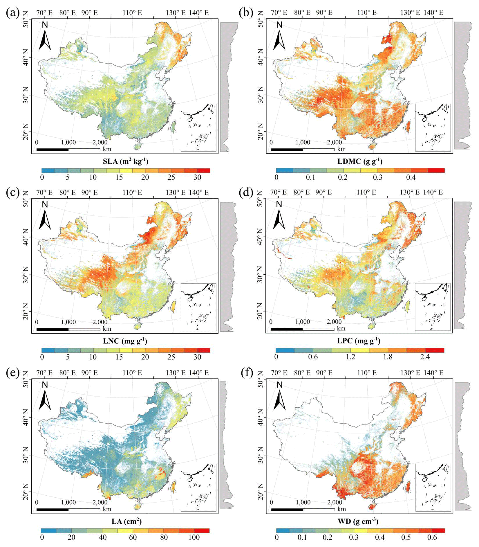
Figure C2 Spatial distributions of plant functional traits based on boosted regression trees. The grey curves on the right of the maps are the trait distribution along with the latitude. The white areas represent the artificial land cover types and bare vegetation.

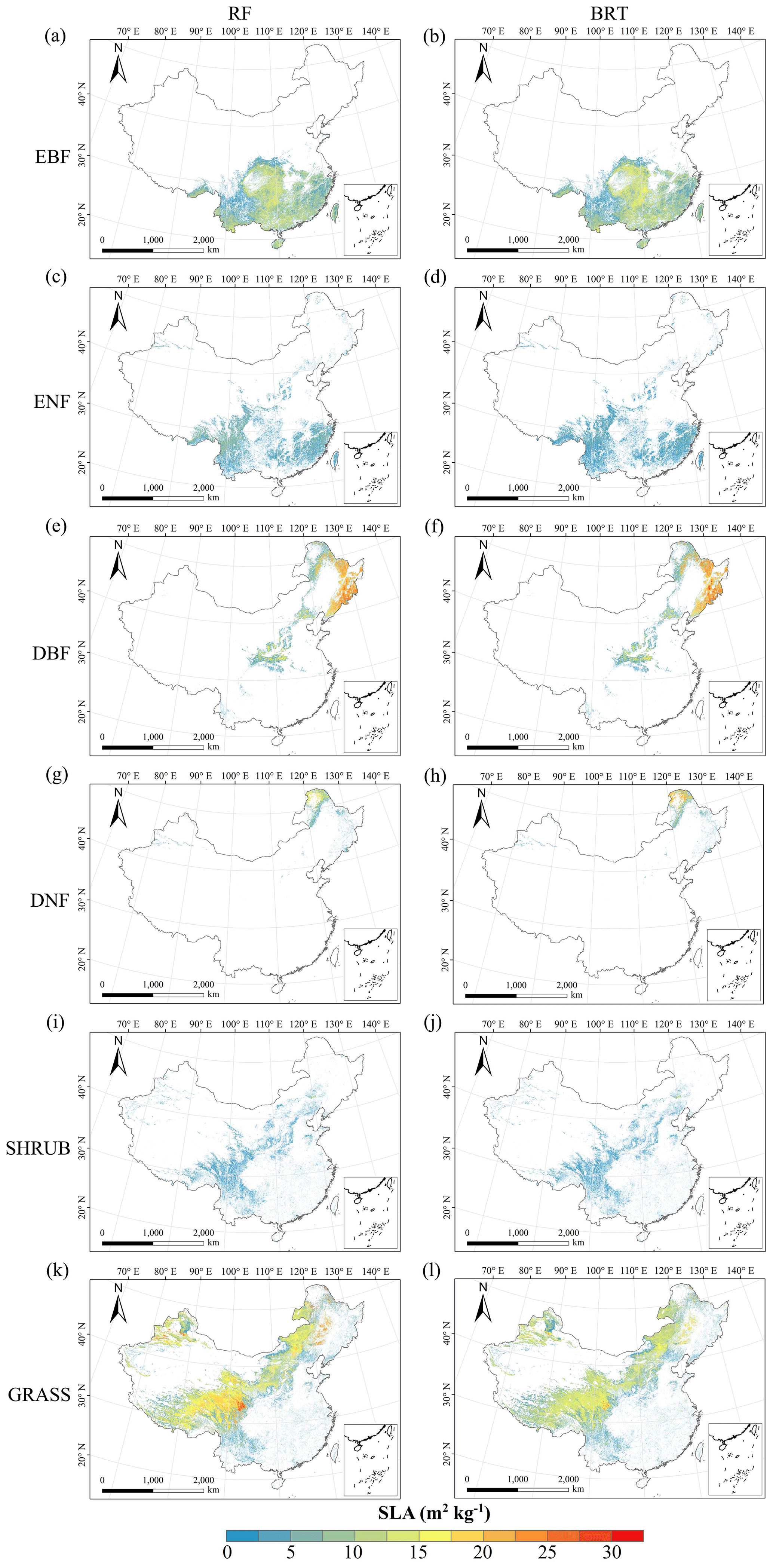
Figure C3 Spatial distribution of the SLA for each plant functional type. The left column is obtained with the RF method, and the right column is obtained with the BRT method. The white areas represent other natural vegetation types and artificial land cover types. EBF: evergreen broadleaf forest; ENF: evergreen needleleaf forest; DBF: deciduous broadleaf forest; DNF: deciduous needleleaf forest; SHRUB: shrubland; GRASS: grassland.

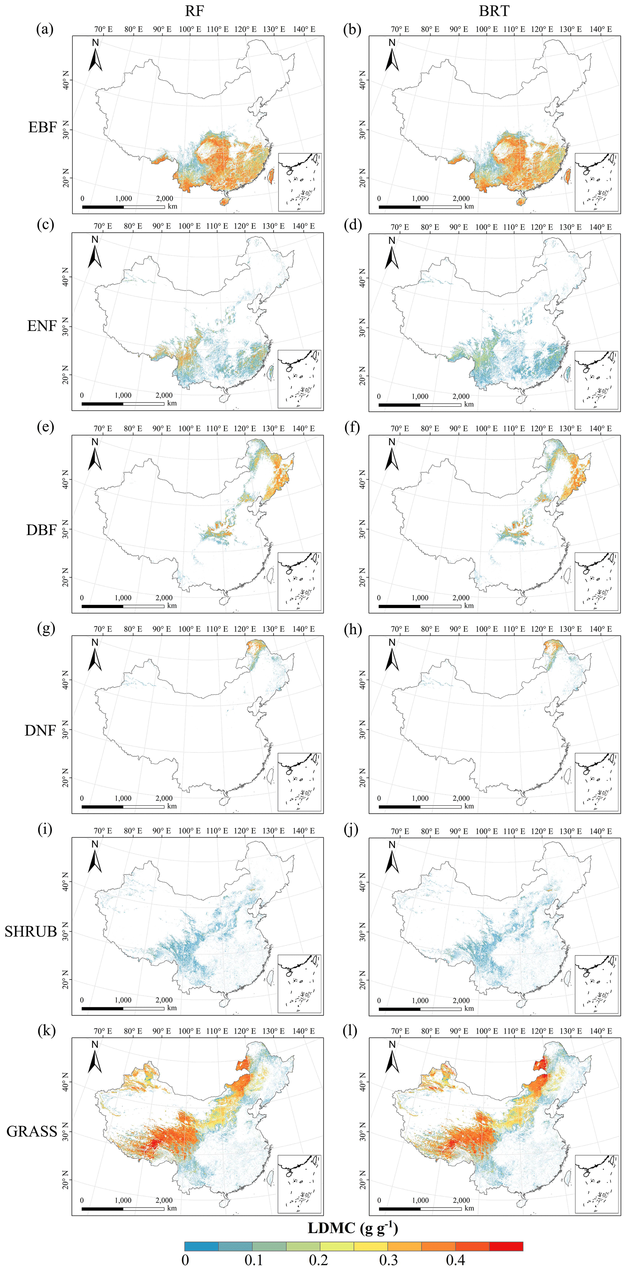
Figure C4 Spatial distribution of the leaf dry matter content (LDMC) for each plant functional type. The left column is obtained with the RF method, and the right column is obtained with the BRT method. The white areas represent other natural vegetation types and artificial land cover types.

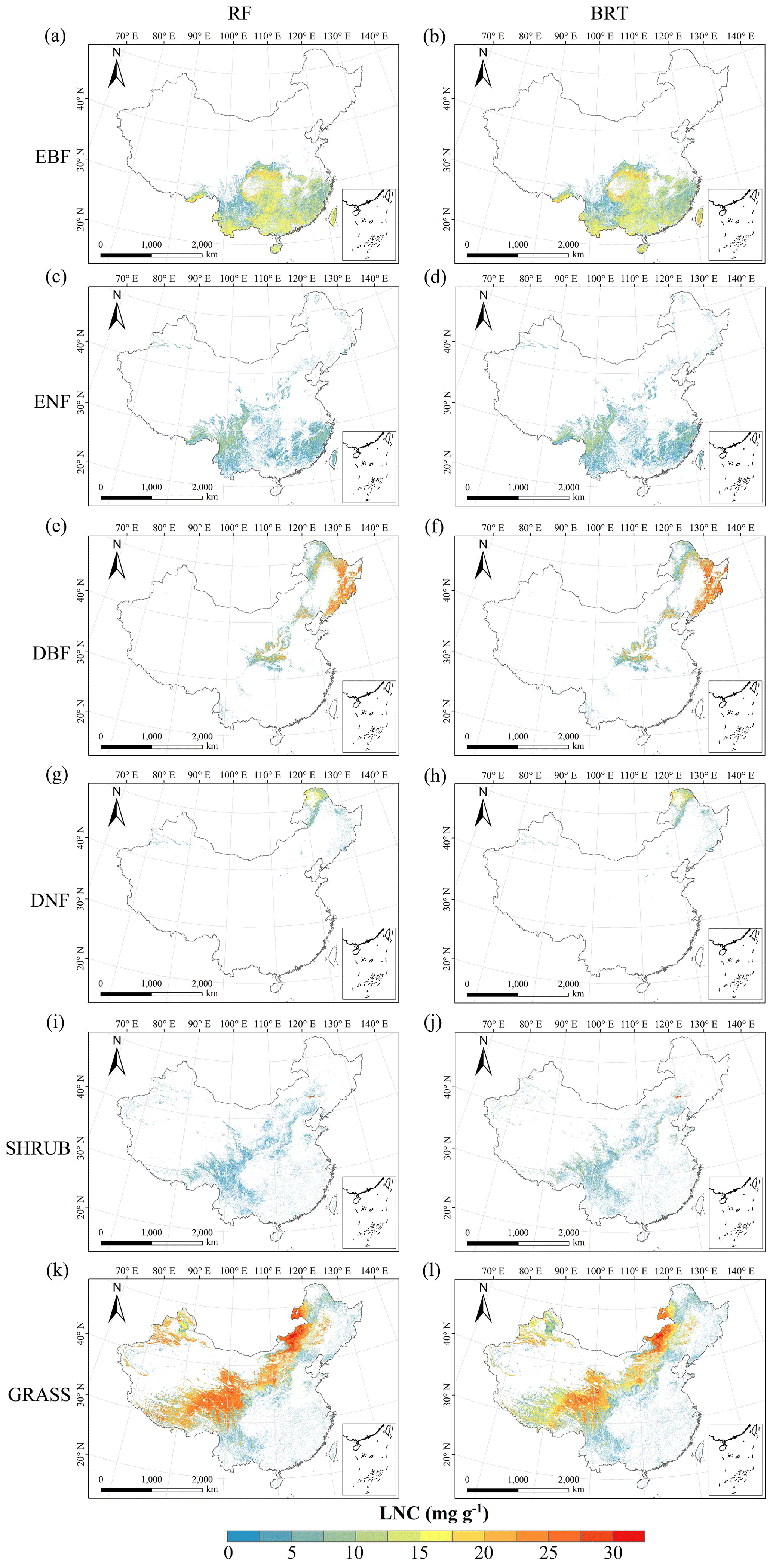
Figure C5 Spatial distribution of the leaf N concentration (LNC) for each plant functional type. The left column is obtained with the RF method, and the right column is obtained with the BRT method. The white areas represent other natural vegetation types and artificial land cover types.

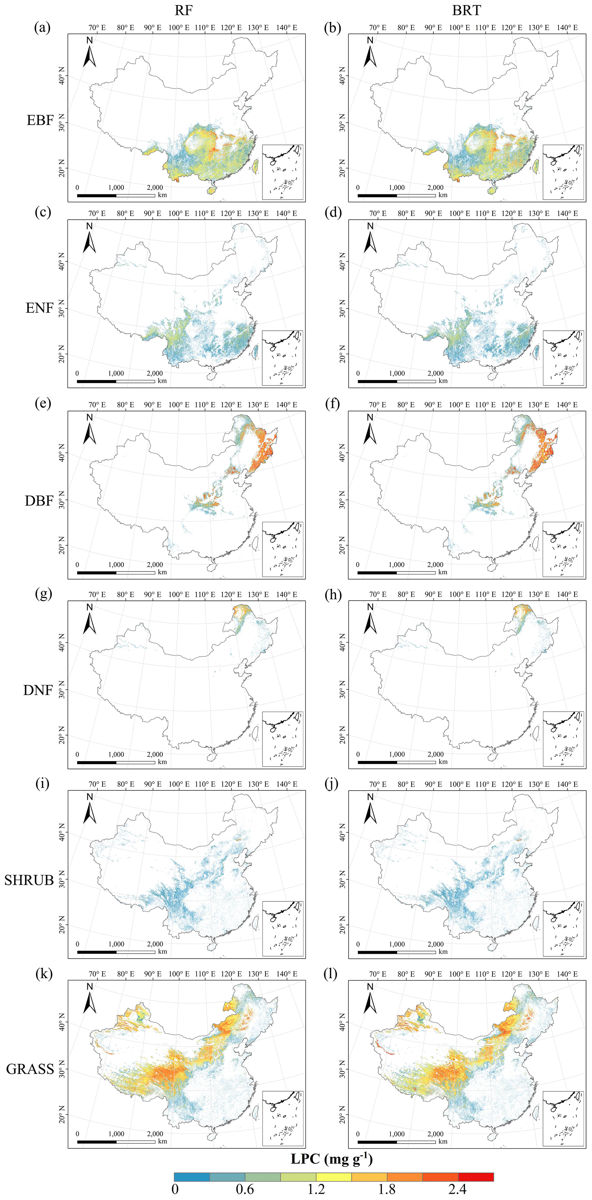
Figure C6 Spatial distribution of the leaf P concentration (LPC) for each plant functional type. The left column is obtained with the RF method, and the right column is obtained with the BRT method. The white areas represent other natural vegetation types and artificial land cover types.

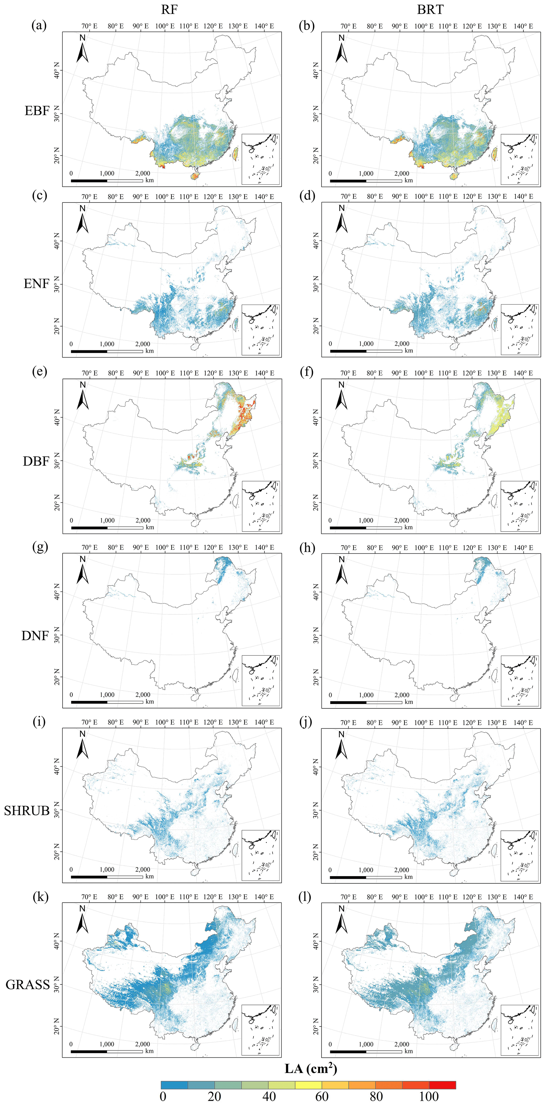
Figure C7 Spatial distribution of the leaf area (LA) for each plant functional type. The left column is obtained with the RF method, and the right column is obtained with the BRT method. The white areas represent other natural vegetation types and artificial land cover types.

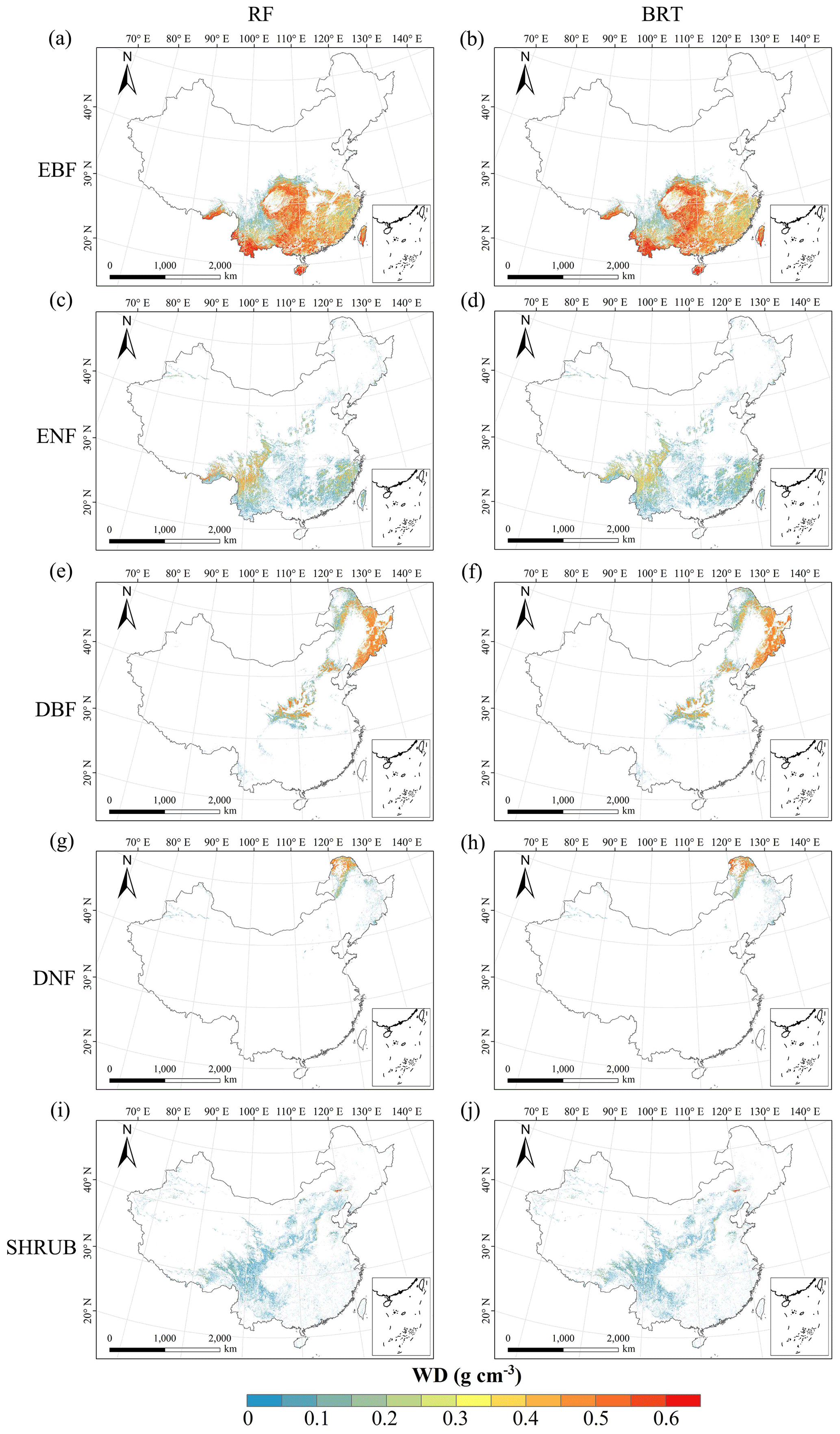
Figure C8 Spatial distribution of the wood density (WD) for each plant functional type. The left column is obtained with the RF method, and the right column is obtained with the BRT method. The white areas represent other natural vegetation types and artificial land cover types.

Appendix D

Figure D1 The relationships between SLA, LDMC, LNC, LPC and their eight most important predictors.

Figure D2 The relationships between LA, WD and their eight most important predictors.

Appendix E: Comparisons between our study and trait maps from previous studies

Given that the trait maps predicted for China were not available from the literature and their authors, we compared our study with those studies performed at the global scale (Table E1). Thus, we extracted the data in China from global trait maps. Before the quantitative comparisons with previous studies, we performed two steps to make the data products as comparable as possible and to improve the consistency between different studies. First, due to the different spatial resolutions of the global trait maps (mainly 0.5°) and our study, we resampled the data products of previous studies and our maps to 0.5° spatial resolution. In addition to Vallicrosa et al. (2022) generating the global maps of LNC and LPC with 1 km spatial resolution, we also compared the frequency distribution of Vallicrosa et al. (2022) with that of our study at 1 km spatial resolution. Second, our study focused on natural vegetation, so the global trait maps were used to filter out nonnatural vegetation (e.g., croplands). For example, Madani et al. (2018) predicted the spatial distribution of SLA that included croplands. We quantitatively compared our maps with previous studies from two perspectives. The comparisons between trait maps were made using frequency plots and spatial correlation (Figs. 7 and E1, Table 4). The maps of the spatial differences between our study and previous studies are displayed as Figs. E2–E6 in Appendix E.

Table E1 Summary of the related trait maps of the previous studies used in this study.

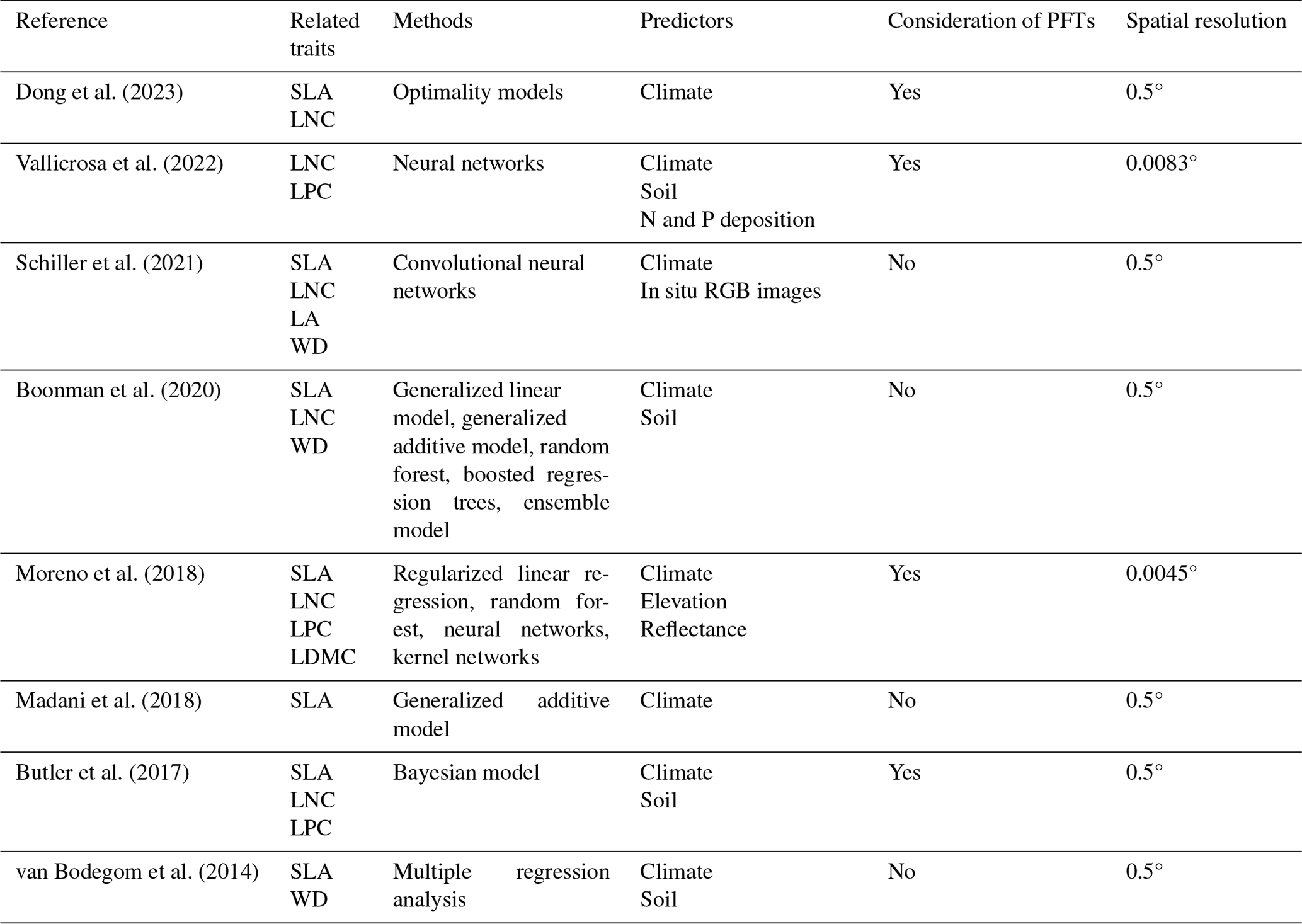
The resolutions 0.5, 0.0083 and 0.0045° correspond to square grid cell sizes of about 50 km, 1 km and 500 m at the Equator. PFT: plant functional type; SLA: specific leaf area; LDMC: leaf dry matter content; LNC: leaf N concentration; LPC: leaf P concentration; LA: leaf area; WD: wood density.

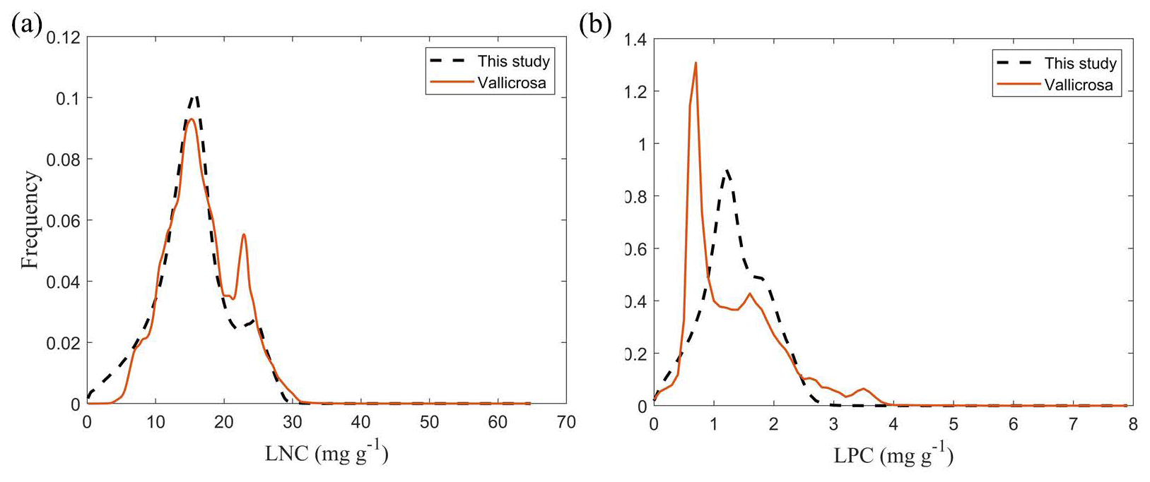
Figure E1 Frequency distributions of the plant functional traits in our study (“This study”, dashed black lines) and Vallicrosa et al. (2022) at 1 km spatial resolution. (a) LNC (mg g⁻¹); (b) LPC (mg g⁻¹).

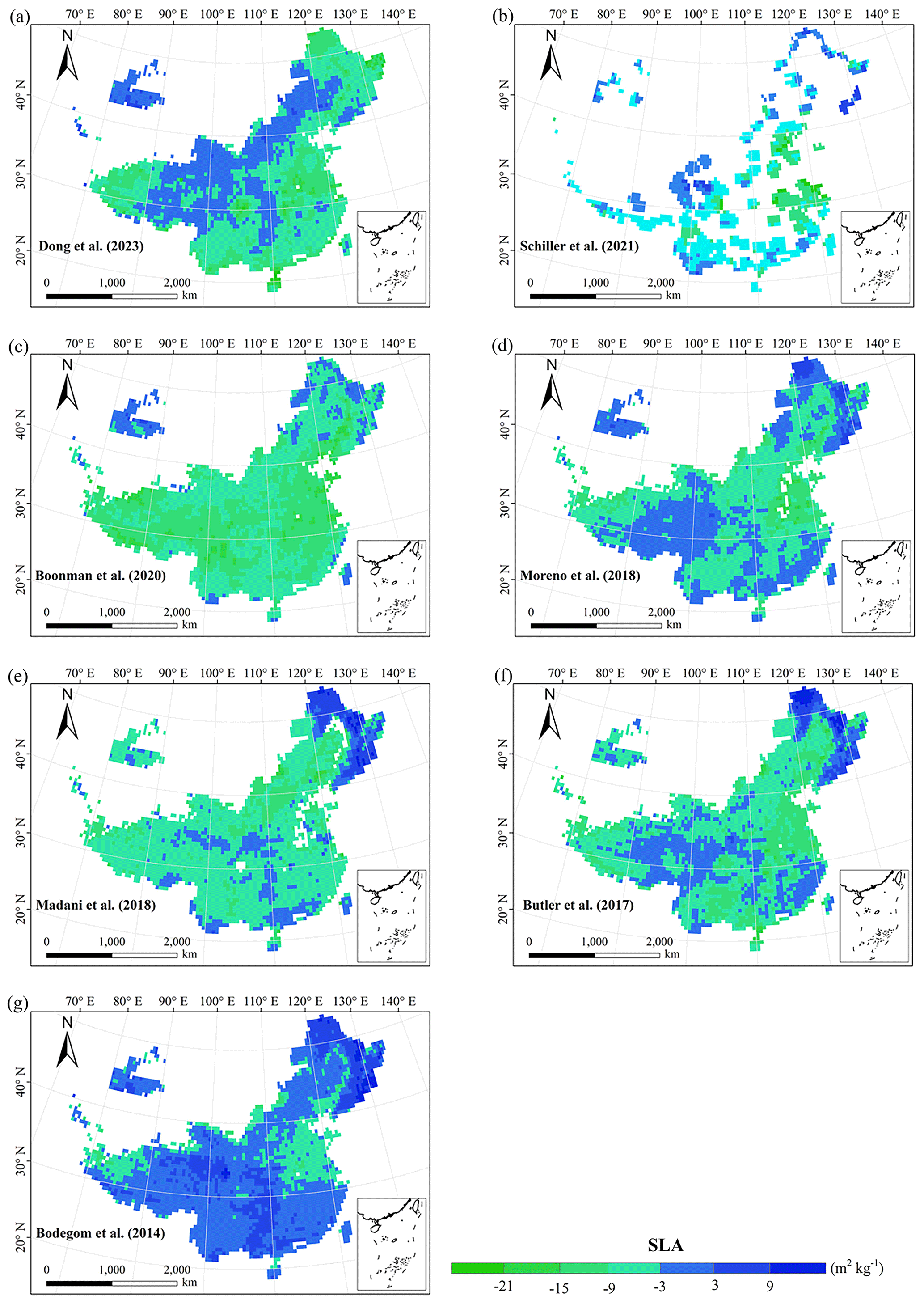
Figure E2 Spatial differences in SLA (m² kg⁻¹) between our study and trait maps from previous studies (see Table E1 for citations).

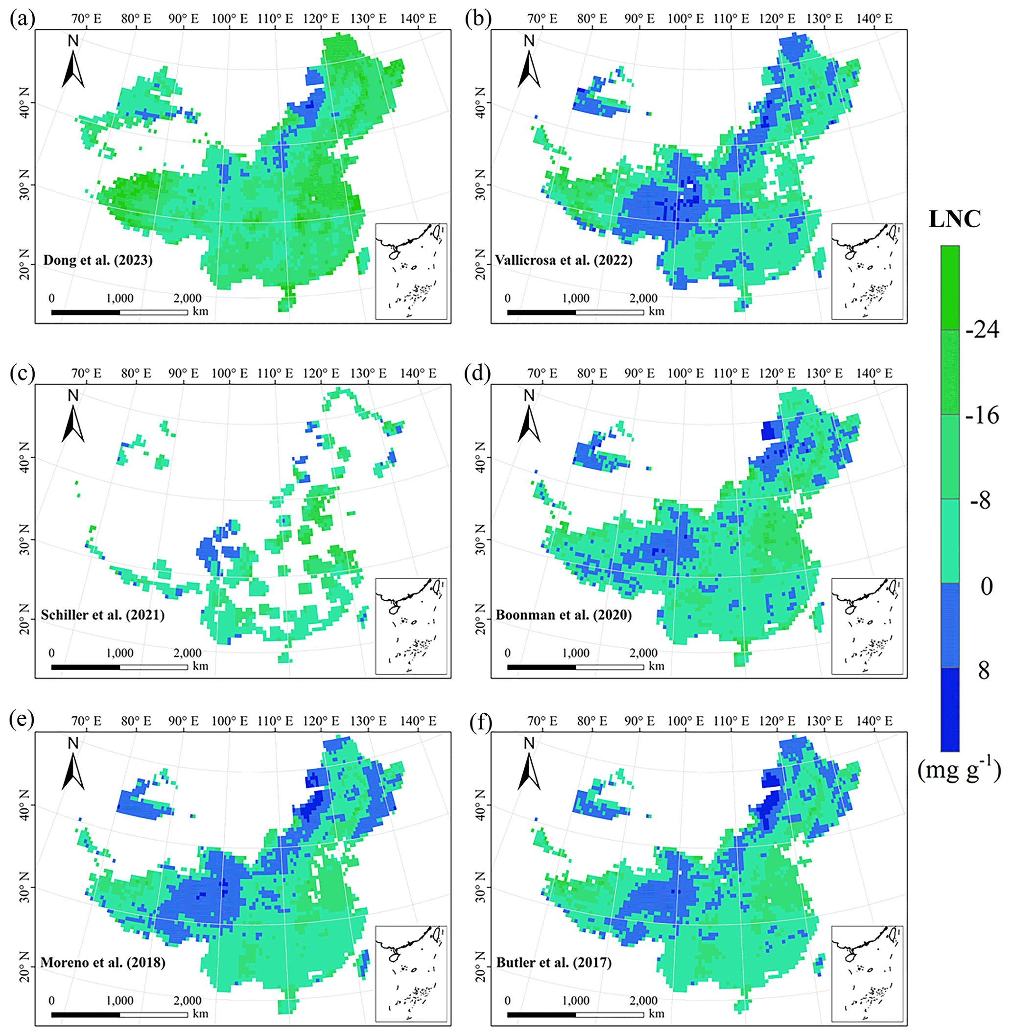
Figure E3 Spatial differences in LNC (mg g⁻¹) between our study and trait maps from previous studies (see Table E1 for citations).

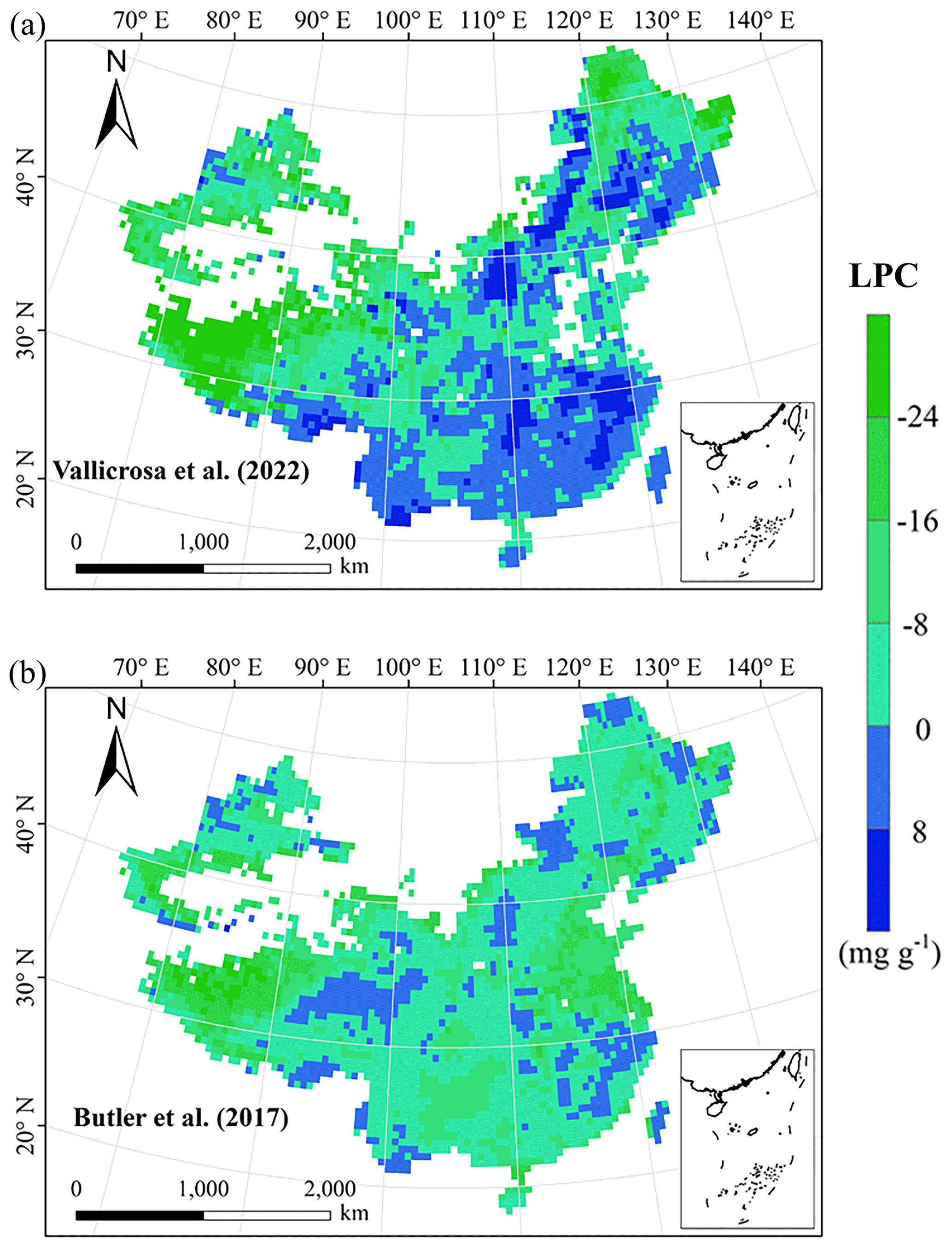
Figure E4 Spatial differences in LPC (mg g⁻¹) between our study and trait maps from previous studies (see Table E1 for citations).

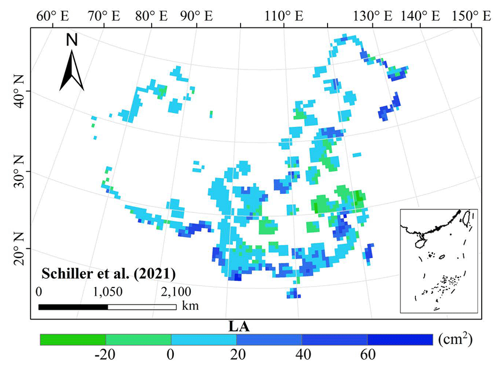
Figure E5 Spatial differences in LA (cm²) between our study and trait maps from previous studies (see Table E1 for citations).

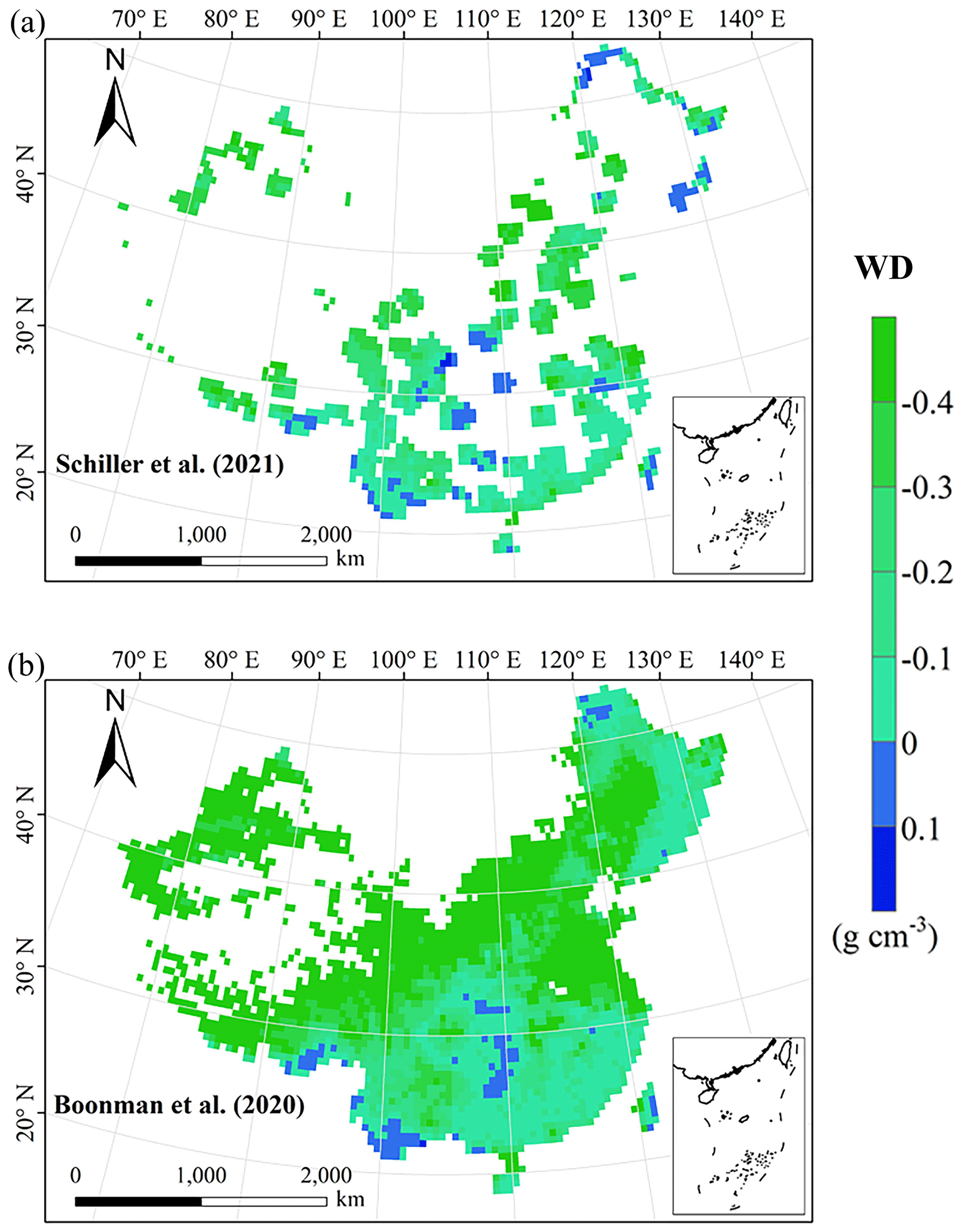
Figure E6 Spatial differences in WD (g cm⁻³) between our study and trait maps from previous studies (see Table E1 for citations).