Air pollution emission inventory using national high-resolution spatial parameters for the Nordic countries and analysis of PM_2.5 spatial distribution for road transport and machinery and off-road sectors

Air pollution is an important cause of adverse health effects, even in the Nordic countries, which have relatively good air quality. Modelling-based air quality assessment of the health impacts relies on reliable model estimates of ambient air pollution concentrations, which furthermore rely on good-quality spatially resolved emission data. While quantitative emission estimates are the cornerstone of good emission data, description of the spatial distribution of the emissions is especially important for local air quality modelling at high resolution. In this paper we present a new air pollution emission inventory for the Nordic countries with high-resolution spatial allocation (1 km × 1 km) covering the years 1990, 1995, 2000, 2005, 2010, 2012, and 2014. The inventory is available at https://doi.org/10.5281/zenodo.10571094 (Paunu et al., 2023). To study the impact of applying national data and methods to the spatial distribution of the emissions, we compared road transport and machinery and off-road sectors to CAMS-REGv4.2, which used a consistent spatial distribution method throughout Europe for each sector. Road transport is a sector with well-established proxies for spatial distribution, while for the machinery and off-road sector, the choice of proxies is not as straightforward as it includes a variety of different type of vehicles and machines operating in various environments. We found that CAMS-REGv4.2 was able to produce similar spatial patterns to our Nordic inventory for the selected sectors. However, the resolution of our Nordic inventory allows for more detailed impact assessment than CAMS-REGv4.2, which had a resolution of 0.1° × 0.05° (longitude–latitude, roughly 5.5 km × 3.5–6.5 km in the Nordic countries). The EMEP/EEA Guidebook chapter on spatial mapping of emissions has recommendations for the sectoral proxies. Based on our analysis we argue that the guidebook should have separate recommendations for proxies for several sub-categories of the machinery and off-road sectors, instead of including them within broader sectors. We suggest that land use data are the best starting point for proxies for many of the subsectors, and they can be combined with other suitable data to enhance the spatial distribution. For road transport, measured traffic flow data should be utilized where possible, to support modelled data in the proxies.

1 Introduction

Air pollution persists as one of the major environmental challenges in the world (Landrigan et al., 2018). Even in the Nordic countries (Denmark, Finland, Iceland, Norway, and Sweden), where the air is considered relatively clean, air pollution causes adverse health effects (Brandt et al., 2013; European Environment Agency (EEA), 2021; Geels et al., 2021; Lehtomäki et al., 2020).

While transboundary air pollution contributes heavily to air quality in the Nordic countries (Im et al., 2019), emissions from low emission height sources often have a large impact on local air quality, especially in the urban areas (Kukkonen et al., 2020; Pisoni et al., 2022). Therefore, when calculating population exposure, the correct representation of local emissions on national or European-scale emission inventories is crucial. There are two important aspects of this: quantitative emission estimates for different emission sources and their spatial distribution. The quality of emission estimates depends on the uncertainties of activity data and emission factors for the different emission sources (European Environment Agency, 2019). For spatial distribution, the ability to represent the location of the emissions is not the only essential issue, but the resolution with which the assessment is carried out is also important (Karvosenoja et al., 2011; Korhonen et al., 2019; Maes et al., 2009; Schaap et al., 2015; Thunis, 2018; Zheng et al., 2017). This study focuses on the spatial distribution of the emissions.

There are few emission sources that can be described with an actual, specific location. Large power and industrial plants have known locations and often significant emissions and can be included in the inventories as point sources with exact coordinates. There are also special cases such as marine traffic, which can be located using tracking systems of actual movement and technical details of the source, for example, the AIS (Automatic Identification System) data (Jalkanen et al., 2009, 2012; Johansson et al., 2017). However, source locations in many cases need to be described using proxies, as the data on the locations of individual sources might not be available, or they do not include enough relevant technical details or other information to estimate the emissions for each source.

Commonly used data for proxies include land cover, road network, and population density data (Geng et al., 2017; Trombetti et al., 2018). Other data sources include satellite observations, for example, for flaring or wildfire emissions, where the emission calculation can also be based on the same data (Böttcher et al., 2021; McCarty et al., 2012). Other, less common, data are also used, such as night-time lights (Zheng et al., 2017). The distribution can be based on single attribute, such as area of the land cover class. Often several spatial datasets are combined to create the proxy, and other data can be used to develop the proxy further. For example, agricultural areas, such as fields, can be combined with animal numbers to distribute emissions from agriculture (Plejdrup et al., 2018). The EMEP/EEA Guidebook chapter on spatial mapping of emissions (European Environment Agency, 2019) proposes three quality levels for spatial proxies for each sector (Tier 3 being most closely related to the spatial activity and Tier 1 the simplest method, the latter only to be used for sources which are relatively unimportant for overall emissions).

Some sectors have more established spatial distribution methods than others. Road transport is an example of such a sector. Road network data, either open source (such as OpenStreetMap) or commercially available, are often used as the basis for the proxy (Kuenen et al., 2022; Li et al., 2017; Romero et al., 2020; Trombetti et al., 2018). Road and street classes can be used to weight the activity on different road types (Zheng et al., 2014). Additional data on, for example, traffic volumes, either measured or based on traffic models, average driving speed, driving patterns, or information on the vehicle fleet composition (Jensen et al., 2008, 2019) allow more detailed weighting. These can help with creating separate proxies for exhaust and dust (resuspension) emissions. The proxy can also be based on bottom-up emission calculation (Andersson et al., 2019; Grythe et al., 2022); i.e. the emissions are calculated on street or even single vehicle level and then aggregated to a grid. It is also possible to calculate the emissions (and, consequently, their spatial distribution) completely by bottom-up methods (Breuer et al., 2020, 2021). For road transport, the EMEP/EEA Guidebook recommends traffic flows, separately per vehicle type, as the Tier 3 level proxy.

Mobile machinery and off-road mobile sources constitute a sector with more complex spatial distribution question as they include a vast number of different types of vehicles and machines that operate in various environments. For example, railways; air traffic landing and take-off (LTO) cycles; and machinery used in agriculture, industry, construction, or maintenance all need very different data to represent the activity spatially. For some of the activities, the choice of proxy data is relatively straightforward. For example, railway emissions can be distributed to a non-electrified railway network or air traffic LTO to airports (and their surroundings). However, for some other types of machinery, for example, the ones used in construction, it is more difficult, as the locations of construction sites change regularly, and GIS data of such activities might not be easily available in consistent forms. A proxy that would represent the activity over several years is hard to develop and would require detailed information on the construction activity over time and data that define the energy used associated with the different phases of the construction project (Lopez-Aparicio and Grythe, 2022).

For different types of machinery, population density is often used as a proxy (Geng et al., 2017), sometimes separated between urban and rural population to cover the differences between those area types (Zheng et al., 2017). However, population data have been shown to be inadequate proxy data for most of the off-road and machinery emissions (Karvosenoja et al., 2020). In general, land use data are often a good starting point for the proxy (for example, fields for agricultural machinery and industrial areas for industrial machinery). Other options include night lights (Zheng et al., 2017) or gross domestic product (Li et al., 2017).

In the EMEP/EEA Guidebook (European Environment Agency, 2019), recommendations for spatial proxies for machinery and off-road sectors are divided between several sectors. Some have their distinct recommendations, such as aviation (airport locations combined with take-off and landing statistics or detailed estimation of emissions by aircraft) and railways (rail network weighted with population or, preferably, diesel rail traffic). Others are combined with stationary combustion (manufacturing industries and construction, commercial, residential, agriculture, other). For all of these, the Tier 1 recommendation is land cover data (or population for manufacturing industries and construction). For industrial and commercial machinery, the guidebook Tier 3 recommendation is related point source data. For residential (household and gardening) and agriculture/forestry, Tier 3 is detailed fuel deliveries accompanied with modelled fuel use estimates based on “population density and/or household numbers and types” and employment data, respectively.

Emissions from the Nordic countries have been assessed nationally and reported as a part of continental-scale emission inventories. The Nordic countries report their official emission inventories according to the United Nations Economic Commission for Europe (UNECE) Convention on Long-range Transboundary Air Pollution (CLRTAP). These inventories are reported as national totals annually and as gridded emissions every 4 years on a 0.1° × 0.1° resolution (approx. 4–6 km (east–west) × 11 km (north–south) for the Nordic area).

The emissions of the Nordic countries are also included in several independent emission inventories. The main examples of global inventories which include spatial distributions of the emissions are the Greenhouse gas – Air pollution Interactions and Synergies (GAINS) model (Klimont et al., 2017) and Emissions Database for Global Atmospheric Research (EDGAR) (Crippa et al., 2018, 2019). Important inventories with regional and global coverage are the CAMS regional and global inventories (CAMS-REG (Kuenen et al., 2022) and CAMS-GLOB-ANT (Doumbia et al., 2021)). Since all these inventories are for either the European or global domain, the spatial distribution is typically based on a more generic methodology which does not take specific Nordic characteristics into account. In the emission estimates themselves however, these can and have been considered as some of these inventories are either built on the national reported emission inventories (CAMS) or actively compared to them (GAINS). The inventories have been used extensively in air pollution impact assessments. The GAMS-REG inventory (and its predecessor TNO MACC-III) has been used in European (Kioutsioukis et al., 2016) and regional-level studies (Belis et al., 2020), as well as in metropolitan regions (Kuik et al., 2016) and for city-scale (Ramacher et al., 2021) modelling. Therefore, the GAMS-REG inventory is a good comparison dataset for more detailed and regionally specific inventories.

A larger-scale inventory can also be comprised of several independent inventories. Li et al. (2017) describe a mosaic approach, in which several national and/or regional-level inventories are combined into one. The source sectors, pollutants, and spatial and temporal resolutions are normalized to create a harmonized dataset. The strength of such an inventory is the possibility of using state-of-the-art available data for each region included in the dataset. HTAP_v3 mosaic (Crippa et al., 2022) is an example of such an inventory, combining national and independent inventories to create a global emission dataset.

In this paper we present a new air pollution emission inventory for the Nordic countries with high-resolution spatial allocation (1 km × 1 km). The country total emissions are based on official national inventories, and the spatial allocation was done separately for each country, and combined into a single, mosaic inventory. The final inventory is compared to a European-scale emission inventory to study how national assessment affects the spatial distribution of the emissions. The comparison is done for two major area source sectors with low emission height, i.e. road transport and machinery and off-road mobile sources. The third major sector, residential wood combustion, was analysed in a separate paper (Paunu et al., 2021). The research questions of this paper are as follows:

1. How does a European level inventory describe emissions in the Nordic countries for road transport and machinery and off-road sectors compared to our more detailed national level inventory?

2. What data are needed for high-quality spatial distribution of air pollution emissions of road transport and machinery and off-road, and how does the EMEP/EEA Guidebook cover them?

2 Methods

Our common Nordic (Denmark, Finland, Iceland, Norway, and Sweden) inventory (Paunu et al., 2023) was compiled using country total emissions from national emission inventories that the countries submit to the CLRTAP. Our inventory was based on the 2016–2018 submissions. Two modifications were made: (1) road transport non-exhaust PM emissions were adjusted to better conform with Nordic traffic dust assessments (Denby et al., 2013; Norman et al., 2016); and (2) for organic carbon (OC) emissions, that are not included in the inventories, rough estimates were calculated based on expert estimates on OC $/$ PM_2.5 ratios on main SNAP (Selected Nomenclature for Air Pollution) levels. The inventory contains annual emissions for 1990, 1995, 2000, 2005, 2010, 2012, and 2014. Components included in the inventory are particulate matter (PM₁₀ and PM_2.5), black carbon (BC), OC, sulfur oxides (SO_x), nitrogen oxides (NO_x), carbon monoxide (CO), non-methane volatile organic compounds (NMVOCs), and ammonia (NH₃). The gridding was done separately for each country, using national data and gridding methods (details are given below). The spatial proxies used in the two studied sectors, road transport and machinery and off-road mobile sources, are presented in Tables 1 and 2, respectively. Spatial proxies for other SNAP sectors are presented in Table S1 in the Supplement. The emissions were harmonized to the same sector nomenclature, i.e. SNAP, and to the EEA reference grid. Spatial resolution for the inventory is 1 km × 1 km in the European grid, ETRS89-LAEA (EPSG: 3035). Large point source emissions are provided with locations and stack heights included. The inventory was originally created for the NordicWelfAir project (Frohn et al., 2022; Lehtomäki et al., 2020), which determined the years and pollutants included. The main aim of developing this new inventory was to provide air pollution modellers and health scientists a harmonized dataset to be used in studies on the link between air pollution exposure and negative impacts on human health.

Table 1 Spatial proxies used for road transport emissions in the Nordic countries.

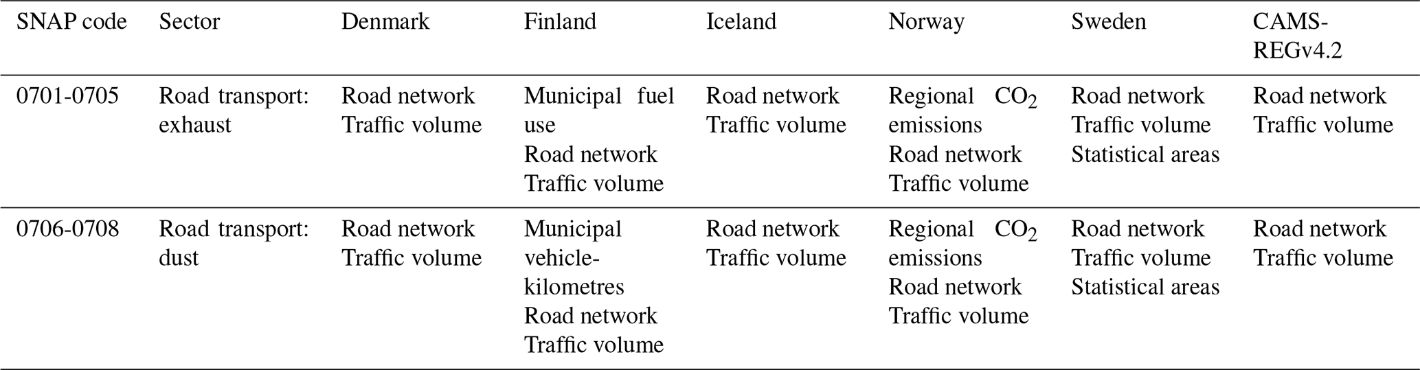
Table 2 Spatial proxies used for machinery and off-road emissions in the Nordic countries. NA – not available

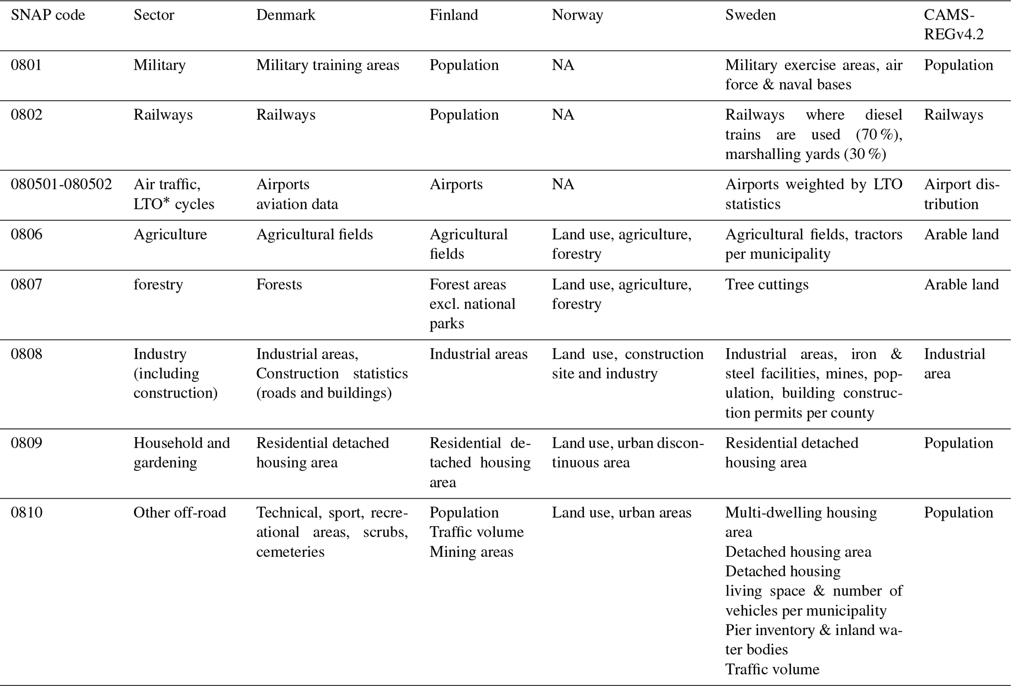
^* Landing and take-off.

Table 3 PM_2.5 emissions and share of national sectoral total for road transport and machinery and off-road subsectors in the Nordic inventory for 2014.

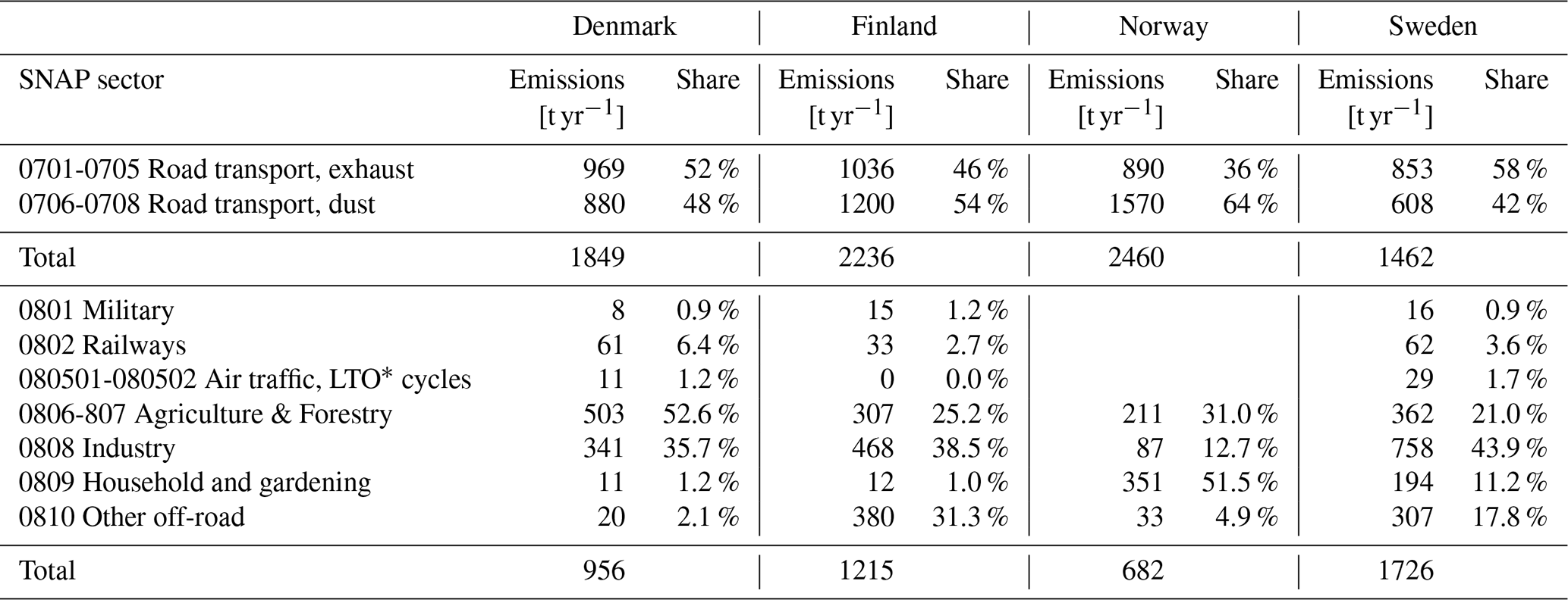
^* LTO: landing and take-off.

2.1 National emissions

2.1.1 Denmark

The spatial distribution of the emission inventory for Denmark was based on the Danish model system SPREAD (Plejdrup et al., 2021). The SPREAD model uses an orthogonal grid with a spatial resolution of 1 km × 1 km covering the Danish area defined by the national border on land and the exclusive economic zone (EEZ) on sea. The model includes spatial distribution keys (GeoKeys) for emissions sources on the most disaggregated sectoral level possible. The GeoKeys are based on plant-specific data when available and otherwise on proxy data.

The main data sources for the GeoKeys are the building and dwelling register (BBR); the Central Husbandry Register (CHR); the fertilizer accounts; the General Agricultural Register (GLR); data from the Danish Association of Chimneysweepers (SFL); the national topographic object oriented map KORT10; the GIS-based National Road and Traffic Database (NRTD); and national statistics including a spatial element, for example, municipality. All GeoKeys are described in Plejdrup et al. (2021).

The distribution of emissions from small combustion plants is based on detailed data from the SFL, including number and type of installation on address level. For residential wood combustion (RWC), this has been combined with information from local studies to apply weighting factors for appliance types (stove and boiler) and building type (permanent residence, apartment, and holiday house). The methodology is described in Plejdrup et al. (2016).

The NRTD includes mileage data per road segment for the Danish road network collected from a large number of local data (Jensen et al., 2019). The model includes five road types and four vehicle types, which are aggregated to three road types and three vehicle types in SPREAD to match the categorization in the emission reporting. Data are included for every fifth year during 1960–2020.

Machinery and off-road emissions comprise a number of sources with separate spatial distributions and proxy data. Emissions from military machinery are allocated to training areas for land-based machinery and to the Danish territory for military aviation. Railway lines are used as a proxy for rail transport, and a 5 km buffer zone around the major airports is used as a proxy for LTO. The distribution for machinery in agriculture and forestry is based on the Danish land use matrix. Land use data are used as a proxy for commercial/institutional, residential, and industrial machinery based on KORT10. For residential machinery, the land use category “residential detached housing area” is used.

The distribution for the agricultural sector is based on detailed data from different agricultural registers. The number of animals by type per farm from the CHR is used for GeoKeys for manure management. The GLR holds information about the fields that are applied for subsidies, the location and size of the fields, and the crops grown on the specific field. These data, in combination with information on the use of fertilizers (animal manure, inorganic fertilizer and other N-containing materials, for example, sludge) from the fertilizer reports, are used to prepare GeoKeys for agricultural soils.

All emissions included as large point sources in the Danish emission inventory, and point sources where plant-specific data are available, are treated as point sources in the SPREAD model, and the emissions are allocated to the exact location. Among the data sources for point sources are EU-ETS reports, annual accounts for individual companies and plants, and the annual database from the Danish Energy Agency (DEA), holding fuel consumption and technology information separately for each district heating or power production plant.

2.1.2 Finland

The spatial distribution of the emission of Finland was based on the Finnish Regional Emission Scenario (FRES) model (Karvosenoja, 2008). Spatial resolution of the FRES model is 250 m × 250 m, from which the emissions were aggregated to the 1 km × 1 km resolution for the Nordic inventory.

Main data sources for spatial proxies for the Finnish emissions are CORINE Land Cover (CLC) 2012 data (European Union, 2012), the Finnish Building and Dwelling Register (BDR), and the national road and street database Digiroad. Spatial distribution of residential wood combustion is presented in Paunu et al. (2021). For road transport (Table 1), national emissions are first distributed to municipalities with municipal fuel use data (for exhaust emissions) and vehicle-kilometre data (for non-exhaust, i.e. traffic dust). Distribution is done separately for trucks, buses, vans, and passenger cars using vehicle-type-specific data. From municipal emissions to grid, road locations from Digiroad are combined with measured traffic volume from Digiroad (for highways) or relative street-class-specific traffic volumes based on municipal traffic counts (for streets). For agriculture, emissions from animals are distributed to municipalities according to animal numbers and to the grid according to field area. Other agriculture emissions are distributed by field area. Emissions from peat production are distributed according to peat production area.

Emissions from the machinery sector are a combination from several subsectors (Karvosenoja et al., 2020). For spatial distribution, the emissions were compiled into 11 subsectors. SNAP sectors 0808 and 0810 for industrial and other off-road sources, respectively, were regrouped into industrial machinery, other off-road, street maintenance machinery, road maintenance machinery, and mining machinery. Proxies used are presented in Table 2. Most subsectors were distributed with land use data using the area of the land use class as the proxy. Street and road machinery used roads and traffic volumes, the same data as the road transport sector. Few subsectors were distributed with population data, as other suitable proxy data were not identified at the time.

Point source emissions for Finland were calculated using the FRES model. The calculation was based on the average annual fuel use or production of the power and industrial plants. The annual value was defined individually for each year, based on the 3-year annual average. The total sectoral emissions were compared to the official national inventory, and remaining emissions were divided into municipalities according to fuel use of small municipal energy production facilities and treated as point sources in the centre of the municipality.

2.1.3 Iceland

The emission inventory for Iceland covers road transport (exhaust and road wear) and point source emissions. Road transport represents the main air pollution source for the capital area and point sources such as aluminium smelters and geothermal power plants for the whole country. In contrast to other Nordic countries, residential wood combustion is rare, and mainly occurs to create a cosy atmosphere (“hygge”) in some recreational houses. Data on machinery and construction sites were lacking and were thus not included.

Road transport exhaust emissions were based on the national inventory, except for PM emissions, which were based on Emissions Database for Global Atmospheric Research (EDGAR) (Crippa et al., 2018) for the year 2008. Non-exhaust emissions were calculated by weighting results from SIMAIR tool for Sweden. The SIMAIR is an online tool for assessing air pollution for Swedish municipalities (Gidhagen et al., 2009). The spatial distribution of the road transport emissions was based on traffic modelling (Hreggviðsson, 2012).

2.1.4 Norway

The emission inventory for Norway was developed specifically for this study, and we prioritized the most relevant sectors for air pollution and population exposure. The selected sectors were combustion in energy and transformation industries (SNAP1); combustion in manufacturing industry (SNAP3); production processes (SNAP4); residential heating (SNAP2) focusing on wood burning emissions, solvent, and other product use (SNAP6); road transport (SNAP7); agriculture (SNAP10); and other mobile sources and machinery (SNAP8), focusing on mobile combustion machinery in manufacturing industries and construction, commercial/institutional, household and gardening, and agriculture/forestry/fishing.

Emissions from SNAP1, SNAP3, and SNAP4 were obtained from the Norwegian Pollutant Release and Transfer Register (NO PRTR) and were spatially distributed based on the exact location of the large point sources provided by the Norwegian Environment Agency. Emissions from residential heating (SNAP2) are largely dominated by wood burning in small-scale combustion for residential heating. Emissions were estimated based on wood consumption data per type of technology (i.e. open fireplace, closed wood stove produced before 1998, and closed wood stove produced after 1998) at county level from Statistics Norway for each year, emission factors developed for Norwegian conditions (Seljeskog et al., 2013), and a dwelling number at 250 m resolution for each emission year (for more details, see Paunu et al., 2021).

National emissions from on-road transport (SNAP7) were spatially distributed on the road network using data from the Norwegian Road Administration and were gridded at 1 km × 1 km. The spatial distribution was based on (1) CO₂ emissions at a regional level, (2) the ratio of the pollutant of interest to CO₂ at a national level for heavy- and light-duty vehicles (HDVs and LDVs), and (3) the amount of traffic at the road links expressed as average daily traffic along with the share of HDVs. The CO₂ emission data at a regional level were used as a proxy to account for the heterogeneous distribution of technological vehicle class in the Norwegian geography, and thereafter the emissions were distributed on the road network based on the average daily traffic. Based on the ratio of CO₂ to the pollutant of interest determined at a national level for HDVs and LDVs, weighted by the kilometres driven by passenger cars and other LDVs, we spatially distribute the emissions. In the case of non-exhaust emissions, the same procedure was followed.

Emissions from agriculture (SNAP10) were distributed using land use data classified as agriculture in CORINE Land Cover 2006 (European Union, 2006). Emissions from other mobile sources and machinery (SNAP8), officially reported under the obligations of CLRTAP, were distributed based on land use classifications: corresponding CORINE land cover classes in the case of construction and industry, urban areas in the case of emissions from commercial/institutional mobile sources, discontinuous urban areas in the case of household and gardening, and agriculture forestry in the case of mobile machinery in agriculture/forestry/finishing.

2.1.5 Sweden

Details of the spatial allocation of Swedish emissions are described in Andersson et al. (2019). For small-scale residential heating, the methodology is also described in Paunu et al. (2021). In general, spatial allocation is made at a low level of aggregation, allowing spatial proxies to be as specific as possible. The spatial resolution or the spatial proxies is 1 km × 1 km, and the spatial reference system is SWEREF99 TM. For use in the Nordic inventory, reprojection was required, resulting in a slightly reduced spatial precision (an increased spatial uncertainty in the range 0–500 m). In total around 60 spatial proxies are combined with statistics at the lowest applicable level of aggregation generating around 100 unique spatial distributions for around 190 emission sectors. In short, road transport emissions have been distributed based on a national bottom-up emission calculation. Traffic flow is based on measurements and a national traffic model provided by the Swedish Road Administration. The composition of the vehicle fleet on each road is based on national statistics from the Swedish Transport Administration and is assigned to each road based on road type, if it is an urban or rural area, and using share of heavy vehicles as described by the national traffic model. Emission factors from HBEFA 3.2 have been used. A minor share of the emissions has not been allocated to individual roads but is instead described for statistical areas employed by the Swedish Road Administration. The bottom-up estimates are updated less frequently than national total emissions. To ensure consistency, the bottom-up estimates for different substances have been gridded at 1 km × 1 km resolution and are used as spatial proxies.

A refined split has been made of total emissions for different types of machinery, allowing separate proxies to be used for each type. For example, for construction machinery, the area of building permits per year is used to distribute emissions between municipalities, and population density within each municipality. For the mining industry, emissions are allocated to mines based on statistics on the total amount of extracted ore. For forestry machinery, a yearly gridded description of the volume of logged wood based on a remote sensing analysis provided by the Swedish Forest Administration is used to allocate the emissions. For agricultural machinery, tractors are distributed between municipalities based on statistics and then allocated to farmland. Machinery used at harbours and airports is distributed between individual locations based on statistics of activity (arrivals or departures). Emissions from road construction machinery are distributed using gridded road work as a proxy.

Trend analysis is carried out for each sector on a regional level to ensure consistency over time in the spatial distribution of emissions. Due to statistical confidentiality, the majority of the point sources are not represented as individual sources but instead included in the gridded emissions. For the point sources that are provided individually, the stack height is estimated based on the size of the emissions.

2.2 Shipping emissions

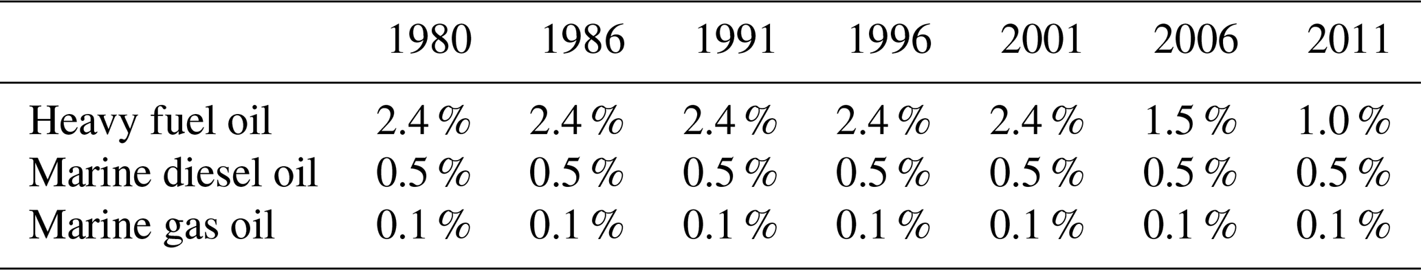
Shipping emissions included in the Nordic inventory were calculated using the Ship Traffic Emission Assessment Model (STEAM) v2 (Jalkanen et al., 2012; Johansson et al., 2013). STEAM describes shipping activity/distribution using positioning data from the AIS (Automatic Identification System). Use of the AIS has increased gradually since its development in the 1990s. Since 2002, the AIS has been required for ships over 300 GT according to IMO (the International Maritime Organization) regulations. The emissions from ships are based on the European 2011 AIS data described in Jalkanen et al. (2016). The 2011 data were used as a starting point (Table 4), and annual emissions were scaled to reflect 1 % growth in CO₂ emissions each year when applied for past years (decreasing future trend run backwards). When fuel sulfur regulations changed in 2010 (Sulfur Directive (EU) 2016/802, IMO MARPOL Annex VI) and the SO_x Emission Control Areas (North Sea (2007), Baltic Sea (2006)) became effective, these impacted SO_x and PM emissions. In the calculations, the fuel type assignment (residuals, distillates) was kept constant, and fuel sulfur content was changed to mimic the effect of sulfur emission control areas (SECAs) (Table 5). Fuel-based emission factors were from the third IMO GHG study, Annex 6, Table 22 (Smith et al., 2014) (assuming an average specific fuel oil consumption of 200 g kWh⁻¹). The fuel mix is assumed constant over the whole time period, with 75 % HFO (heavy fuel oil), 24 % MDO (marine diesel oil), and 1 % MGO (marine gas oil). Before the year 2000, no changes in average sulfur content were assumed. It should be noted that using 2011 ship activity data for Europe and scaling emission totals without considering dedicated sea-area-specific calculations may lead to uncertainties in the emissions. Also, projections of the past, as distant as 30 years, are also prone to significant uncertainty. Our approach aimed to describe the SECA zones more accurately than the non-SECAs.

Changes in NO_x emission factors due to fleet renewal were included by a linear interpolation of NO_x emission factors of old engines to emission factors of new engines. There were large uncertainties in VOC emissions. Assuming gradual technology improvements, estimates in the upper end of the range found in the literature have been applied for older ship engines (0.0023 g g⁻¹ (Entec UK Limited, 2002) and estimates from the lower end for newer engines (0.00045 g g⁻¹ (Cooper, 2001)). Annual growth is assumed to be 1 % yr⁻¹ before year 2000.

Table 4 CO₂-content of different fuel grades applied in estimations for the years 1990–2000 using year 2011 as baseline.

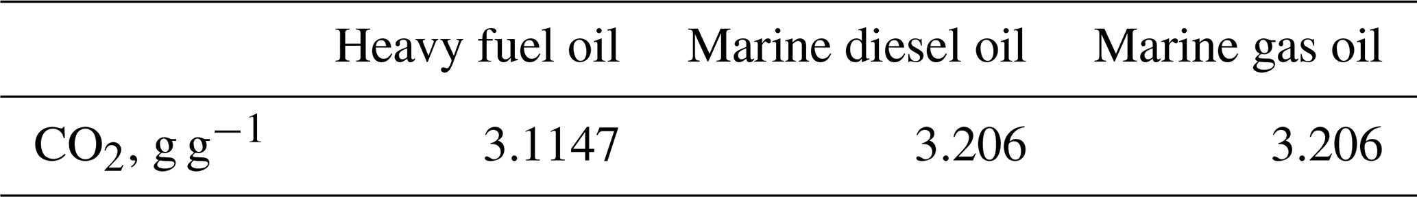
Table 5 Fuel sulfur content applied in estimations of emissions for years 1990–2000 using year 2011 as baseline.

2.3 CAMS-REG v4.2 inventory

CAMS-REGv4.2 is a European-scale emission inventory to support air quality modelling exercises, and version 4.2 covers the years 2000–2017. This inventory is described in detail in Kuenen et al. (2022). To support the policy applications, the inventory relies where possible on the official reported emission data to the Convention on Long-Range Transboundary Air Pollution (LRTAP) as well as the EU National Emission Ceilings Directive (NECD), based on the 2019 submissions. These official reported data are collected from the national reporting of air pollutants and checked for inconsistencies, gaps, and errors. In those cases where for a specific country and pollutant the reported data were found unfit for use, these were replaced with other emission estimates, most notably from the IIASA GAINS model (Amann et al., 2011). The spatial resolution of the inventory is 0.1° × 0.05° (longitude–latitude, roughly 5.5 km × 3.5–6.5 km in the Nordic countries).

The CAMS-REGv4.2 inventory uses the country reported data of the sectoral emissions at a national level, while the spatial distribution is performed using an independent and consistent approach over Europe. This implies that for each sector, a relevant distribution parameter is chosen. For road transport, the spatial distribution of emissions is based on a combination of OpenStreetMap for the road network and Open Transport Map for information on the traffic volumes. The spatial distribution parameters for each detailed sector in the inventory are described in Kuenen et al. (2022) and the supplementary information therein. Shipping emissions at sea in CAMS-REGv4.2 are based on the STEAM model approach (described in Sect. 2.2). CAMS-REGv4.2 uses a more recent version of STEAM (v3.5) than the Nordic inventory introduced in this paper, with more complete AIS datasets and more detailed consideration of regional sulfur rules. For other non-road transport, railway emissions are allocated to a map of the rail lines, whereas airports are assigned to the location of main airports weighted by the number of flights per airport. This is done for each individual year to reflect opening and closure of specific airport sites. For mobile machinery used in industry, emissions are assigned to industrial areas from the Corine Land Cover dataset (CLC2012) (European Union, 2012), whereas for the agriculture sector, the arable land classification from the same dataset is used to spatially disaggregate emissions. Remaining “other” sources are spatially distributed using population density.

2.4 Comparison methods

A statistical comparison between the Nordic and CAMS-REGv4.2 inventories was carried out using the index of agreement developed by Duveiller et al. (2016). The index is non-dimensional, bounded, and symmetric. The index (λ) is calculated as

$$\begin{array}{}\text{(1)}& \mathit{\lambda }=\mathit{\alpha }\cdot r={\displaystyle \frac{\mathrm{2}}{{\mathit{\sigma }}_X/{\mathit{\sigma }}_Y+{\mathit{\sigma }}_Y/{\mathit{\sigma }}_X+{\left(\overline{X}-\overline{Y}\right)}^{\mathrm{2}}/{\mathit{\sigma }}_X{\mathit{\sigma }}_Y}}\cdot r,\end{array}$$

where $\overline{X}$ and $\overline{Y}$ are the mean values of the datasets X and Y, σ_X and σ_Y are their standard deviations, and r is the Pearson product-moment correlation coefficient. α represents how much the index of agreement deviates from the Pearson correlation coefficient. The index also enables the separation of unsystematic and systematic differences, represented by unsystematic index λ_u and systematic noise f_sys. The unsystematic index λ_u represents the value the index λ would take if there was no systematic bias between the datasets (for example one dataset having systematically higher values than the other). The systematic noise f_sys represents the proportion of total deviation caused by the systematic bias. The details of the method and the mathematics can be found in the reference. The index of agreement was calculated with those cells that had non-zero values in either dataset. This reduced the number of no-data cells and highlighted the differences between the datasets.

The spatial comparison was carried for two sectors, road transport and machinery and off-road sectors. The road transport sector is a good example of sector in which the spatial distribution methods are well established, and data are readily available (Table 1). In contrast, the machinery and off-road sector is more difficult due to its heterogeneity and less obvious suitable proxies (Table 2). For the comparison, the Nordic inventory was aggregated to the same resolution as the CAMS-REGv4.2 inventory (0.1° × 0.05°). The comparison was done separately for each country. Furthermore, a visual comparison was done to complement the analysis. The PM_2.5 emissions were compared to assess their role in the analysis of the differences in the spatial distribution. Finally, differences in normalized proxy weight maps were visually analysed. The emissions were normalized separately within each country by dividing the cell values by the total country emission of the sector. The difference maps were then calculated for each country raster.

3 Results

In the following we first present the total emissions and the spatial distributions of road transport and machinery and off-road emissions in the Nordic inventory and thereafter the comparison to the European dataset.

Total Nordic emissions for all pollutants are presented in Fig. 1 (shipping not included). Shipping emissions are presented in Fig. 2. Figure 3 presents the spatial distribution of the total PM_2.5 emissions for 2014 and also shows the spatial coverage of the shipping emissions in the inventory. Spatial distributions of emissions of other pollutants are presented in the Supplement (Figs. S1–S9). Sectoral emissions per country are presented in the Supplement.

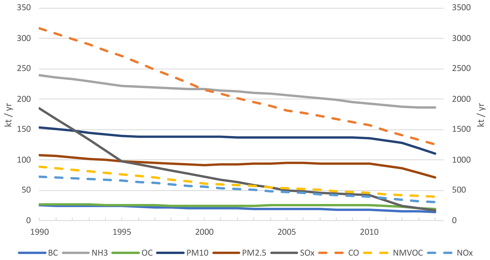
Figure 1 Total Nordic emissions for 1990–2014 (shipping excluded). CO, NMVOC, and NO_x emissions (dashed lines) use the right y axis (which is 10 times the left axis).

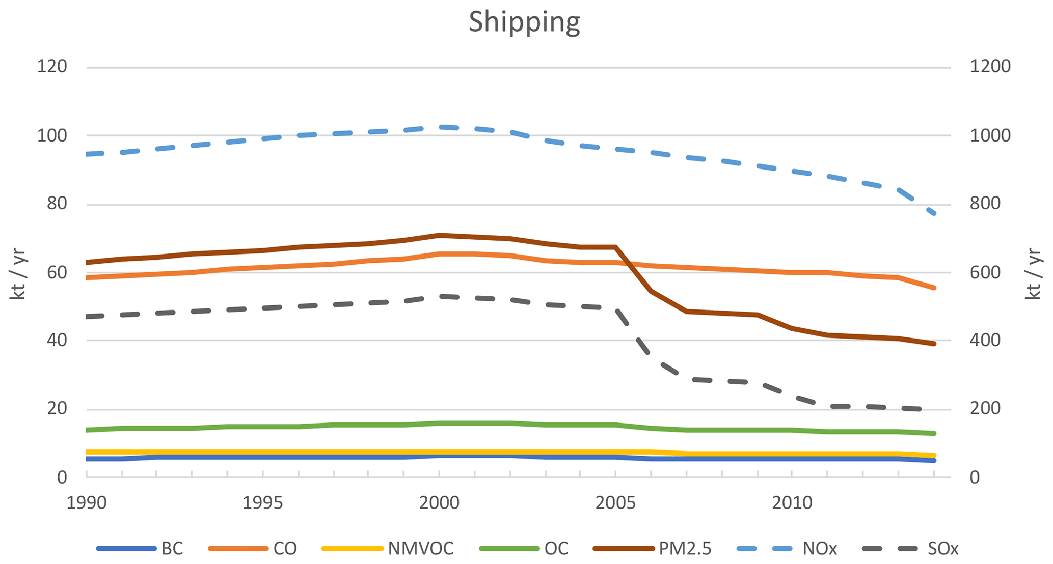
Figure 2 Shipping emissions in the Nordic inventory for 1990–2014. NO_x and SO_x emissions (dashed lines) use the right y axis (which is 10 times the left axis). For spatial extent of the shipping emissions, see Fig. 3.

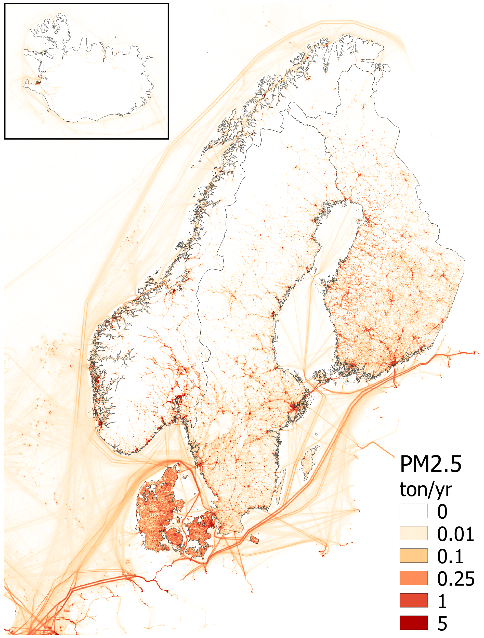
Figure 3 Total PM_2.5 emissions in the Nordic countries in 2014 (except shipping around Iceland in 2010) in 1 km × 1 km resolution. The map also shows the spatial extent of shipping emissions in the Nordic inventory. The legend shows the colours at the exact emissions values, and colours between these values are interpolated.

3.1 Spatial distribution of road transport emissions

Spatial distribution of PM_2.5 emissions from road transport is presented in Fig. 4. The methods and spatial distributions were well aligned between the countries, but there were still differences in the details on how some factors were considered. All countries used road network data and traffic volumes as proxy data. Each country also took the distribution between heavy- and light-duty vehicles into account. Sweden and Norway had two vehicle categories, Denmark used three, and Finland separated the vehicles into four categories (two heavy and two light duty). The countries had separate proxy data for each category. The traffic volume data were measured where possible and modelled to fill the gaps. Often the roads were divided into several types, which then were assigned with relative traffic volumes. Finland and Norway used a two-step process, in which the emissions were first distributed to regional or municipal level and then to the road network within those areas. Finland took the vehicle categories into account on a municipal level, whereas Norway did it on a national and again on a road level. Sweden allocated a minor part of the emissions to larger statistical areas instead of roads, creating large areas with uniform, small emissions. In each country the emissions were concentrated to larger cities and busiest highways, as can be expected. Denmark had the most evenly distributed emissions due to a higher population density, and, thus, higher density of roads, than the other Nordic countries. In all countries the highest emissions were weighted to the capital cities. However, Norway had few high emission cells in all largest cities and the least emissions weighted to roads between cities, leading to higher difference between urban areas and highways. Spatial distributions for road transport exhaust and dust emissions were similar in each country. Finland had different municipal-level proxies for exhaust and dust emissions, the former being based on fuel use and latter on kilometres driven. In practice, the two distributions were very similar.

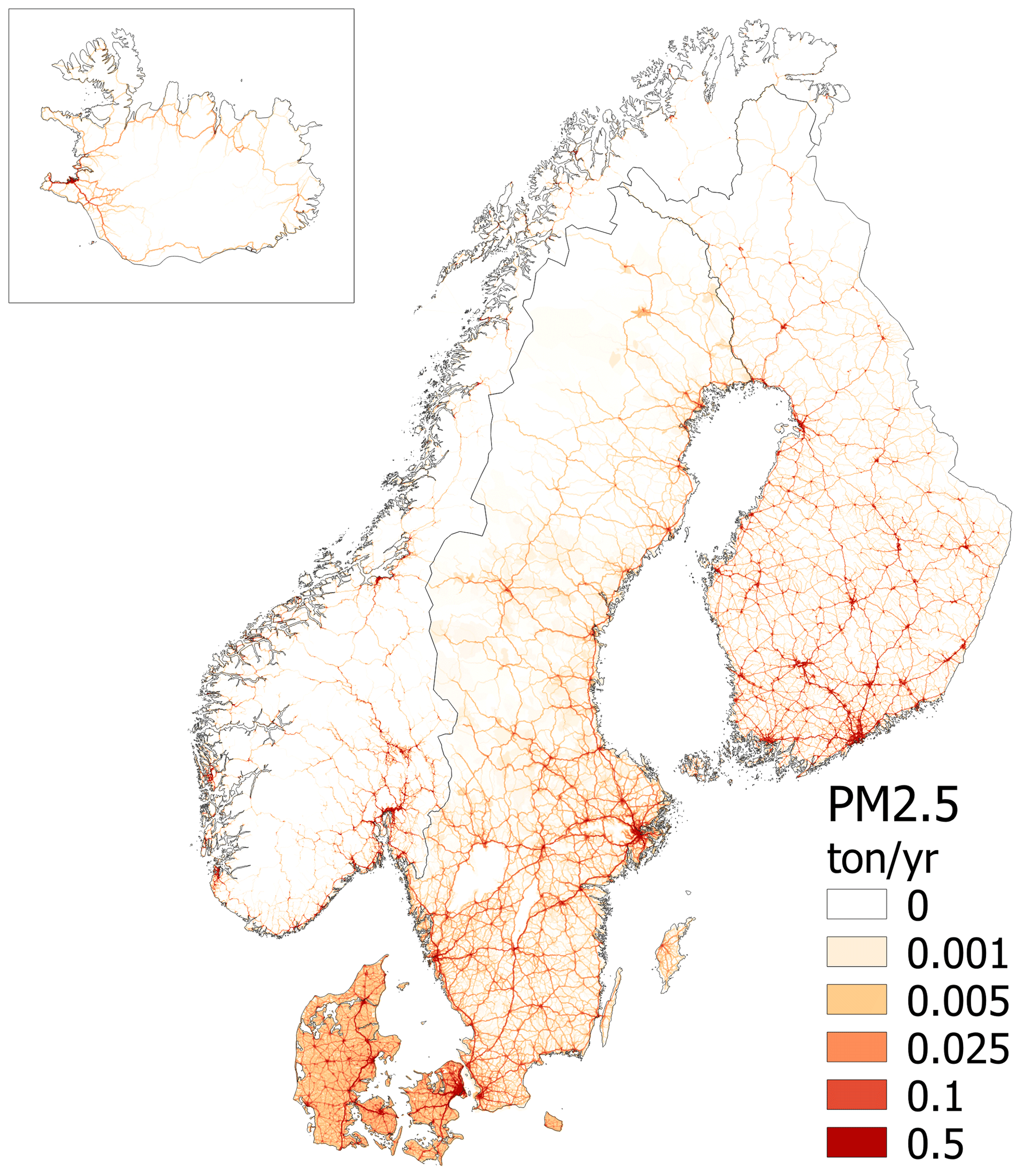
Figure 4 Road transport (SNAP 7) PM_2.5 emissions in the Nordic countries in 2014 in 1 km × 1 km resolution. The legend shows the colours at the exact emissions values, and colours between these values are interpolated.

3.2 Spatial distribution of machinery and off-road emissions

Spatial distribution of PM_2.5 emissions from machinery and off-road is presented in Fig. 5. Table 3 shows the subsectoral emissions and their share of the national total of the sector. Spatial distributions for machinery emissions showed more intricate differences between the countries than road transport emissions. One reason for this was that the machinery and off-road sector that was considered here consists of several heterogenous subsectors and, therefore, contains a multitude of proxies. The proxies used are presented in Table 2. The emission shares of the subsectors were variable between the countries. In 2014, in Denmark, the highest shares of machinery emissions were agriculture and forestry (53 %) and industry (36 %). In Finland, the highest shares were industry (39 %), other off-road (31 %), and agriculture and forestry (25 %). In Sweden, the order was industry (44 %), agriculture and forestry (21 %), and other off-road (18 %). Norway was the only one with the highest share in household and gardening (52 %), followed by agriculture and forestry (31 %). However, there were some differences in the allocation of construction and road maintenance emissions regarding the subsectors (presented in the Table 2). Denmark allocated all of them under industry, but Sweden and Finland included road construction and maintenance under the other off-road sector. While this is mainly a technical detail, it highlights the complexity of the machinery and off-road sector. Even with some differences in the allocation, the shares indicate how the countries differed from each other regarding the estimation of the underlying activities and their emissions.

In all countries the most emissions were weighted to cities. In addition, in Finland roads stood out, and a few mines had high emissions. In Sweden, notable areas were large railway stations and their surroundings, airports, and some mines. In Norway, there were little emissions outside the population centres. Denmark had the most even distribution. Some larger roads, especially in the east, had high emissions on highways due to road construction.

Land use was the most common proxy data used in machinery and off-road. In some cases, statistical data were used to weight the emissions with more than just the area of the land use class. For example, Sweden combined registered tractors per municipality with agricultural field area, and Denmark used construction statistics of roads and buildings. One of the most prominent differences was how roads were used for proxies. Norway did not use road data for machinery, and Finland had the most weight on them of the four countries, apart from a few road segments in Denmark. It is notable that population was used very little as a proxy. Only Finland distributed some maintenance and construction machinery that way.

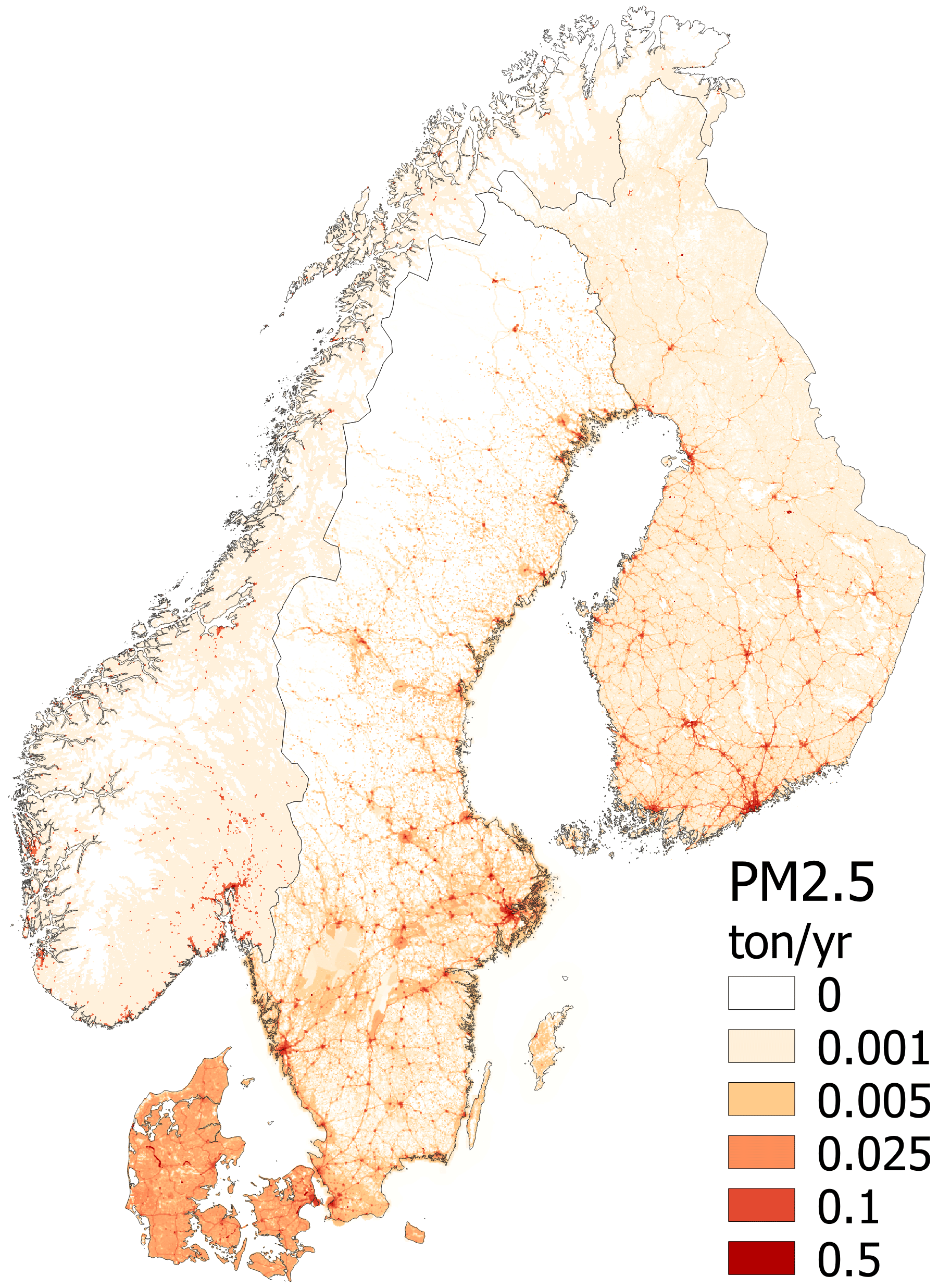
Figure 5 Machinery and off-road (SNAP 8) PM_2.5 emissions in the Nordic countries in 2014 in 1 km × 1 km resolution. The legend shows the colours at the exact emissions values, and colours between these values are interpolated.

3.3 Comparison to CAMS-REGv4.2

3.3.1 Country total emissions

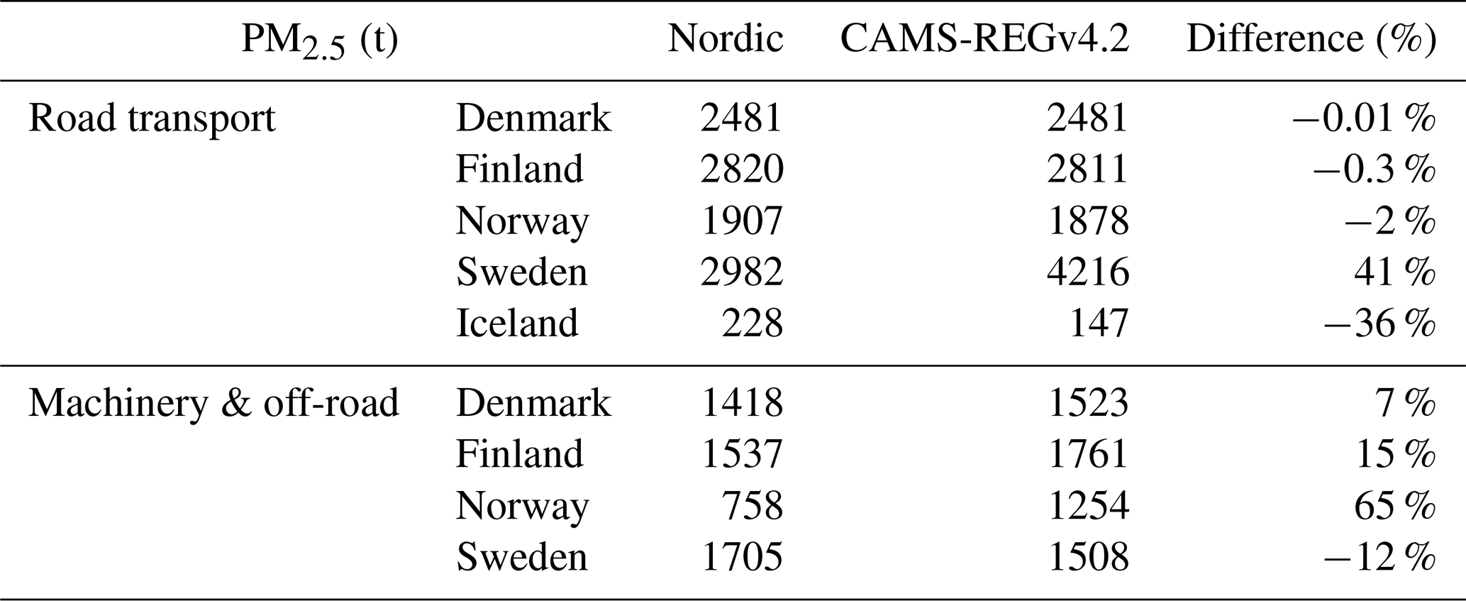
The total national PM_2.5 emissions from road transport and machinery and off-road sectors for 2010 in the Nordic and CAMS-REGv4.2 inventories are presented in Table 6. For road transport, the emissions were similar, except for Iceland and Sweden. In Iceland, the significant difference was related to the use of EDGAR emissions for PM emissions from road transport in the Nordic inventory, whereas the CAMS-REG inventory used the official national inventory results from Iceland. For Sweden, the difference came from traffic dust emissions. These emissions were adjusted in the Nordic inventory from the official reported emissions (as explained in the methods section), and CAMS-REGv4.2 follows the official reported numbers, so the difference came from estimation methods. In this paper we will not go into further details on this, as we focus on the spatial distribution of the emissions.

For machinery the emissions were similar, except for Norway. In Norway, the Nordic inventory focused on the main subsectors and, therefore, lacks emissions from some less significant subsectors. CAMS-REGv4.2 also had higher emission estimates in the household and gardening subsector, where the estimate was as large as the whole sector estimate for Norway in the Nordic inventory.

Table 6 PM_2.5 emissions from road transport and machinery and off-road sectors in the Nordic and CAMS-REGv4.2 inventories for 2010.

3.3.2 Spatial distribution of emissions

The spatial distributions of road transport emissions in the two inventories are presented in Fig. 6 and index of agreement results for the spatial distributions in Fig. 7. Differences in the normalized proxy weights are presented in Fig. 8. The spatial distributions of machinery and off-road emissions are presented in Fig. 9 and index of agreement results for the spatial distributions in Fig. 10.

The index of agreement λ indicated that for road transport, the distributions were similar in Finland, Iceland, and Norway, whereas Denmark had the lowest index of agreement. In Sweden there were two cells which had high emissions but only in one of the inventories. Also, the cells were not close to each other, as in the Nordic inventory the high emission cell was in the centre on Stockholm, and in CAMS-REGv4.2 it was in the centre of Malmö. Without these two cells, the index of agreement results would have been nearly as good as for Finland (with λ=0.724 and λ_u=0.810). These were also the cells with largest differences in the proxy weights between the two inventories in Sweden. The Copenhagen area in Denmark was another region with differences of similar magnitude. In Iceland, the differences were even bigger in Reykjavik (Nordic inventory having higher weight), in Akureyri, and next to Keflavik airport (in both CAMS-REGv4.2 had higher weight).

In all countries, the Nordic inventory had more emissions weighted to the capital areas and highways, while CAMS-REGv4.2 had more weight in other cities and non-urban areas without highways. In Copenhagen this can especially be seen, as the Nordic inventory has more emissions in the city, and CAMS-REGv4.2 on the outskirts. Helsinki had few exceptions, as there, the CAMS-REGv4.2 inventory had much higher weight in the cell containing the city centre and also in one cell in the east (containing a large harbour), and the Nordic inventory had higher weight in the cells containing ring roads. In Finland, and to a lesser degree in Sweden, CAMS-REGv4.2 had more weight in city centres outside the capital metropolitan area. In general, in the continental Nordics, the highest proxy weight differences were in cities and a few busiest highways in Finland and Denmark. Finally, there was a clear difference in the Gotland, where CAMS-REGv4.2 had higher proxy weight and emissions throughout the island.

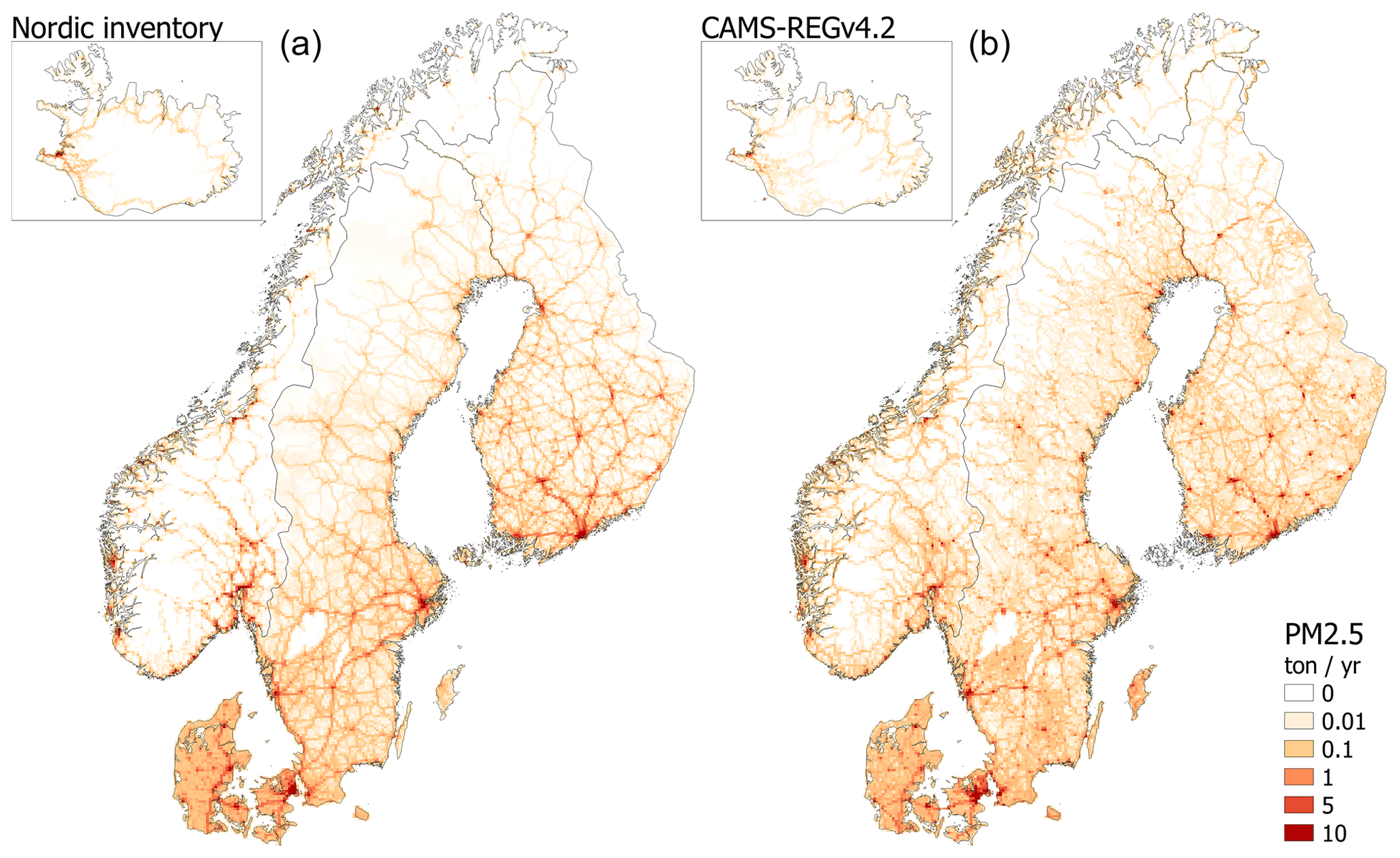
Figure 6 Spatial distribution of road transport PM_2.5 emissions in the Nordic inventory in (a) and CAMS-REGv4.2 in (b). The legend shows the colours at the exact emissions values, and colours between these values are interpolated.

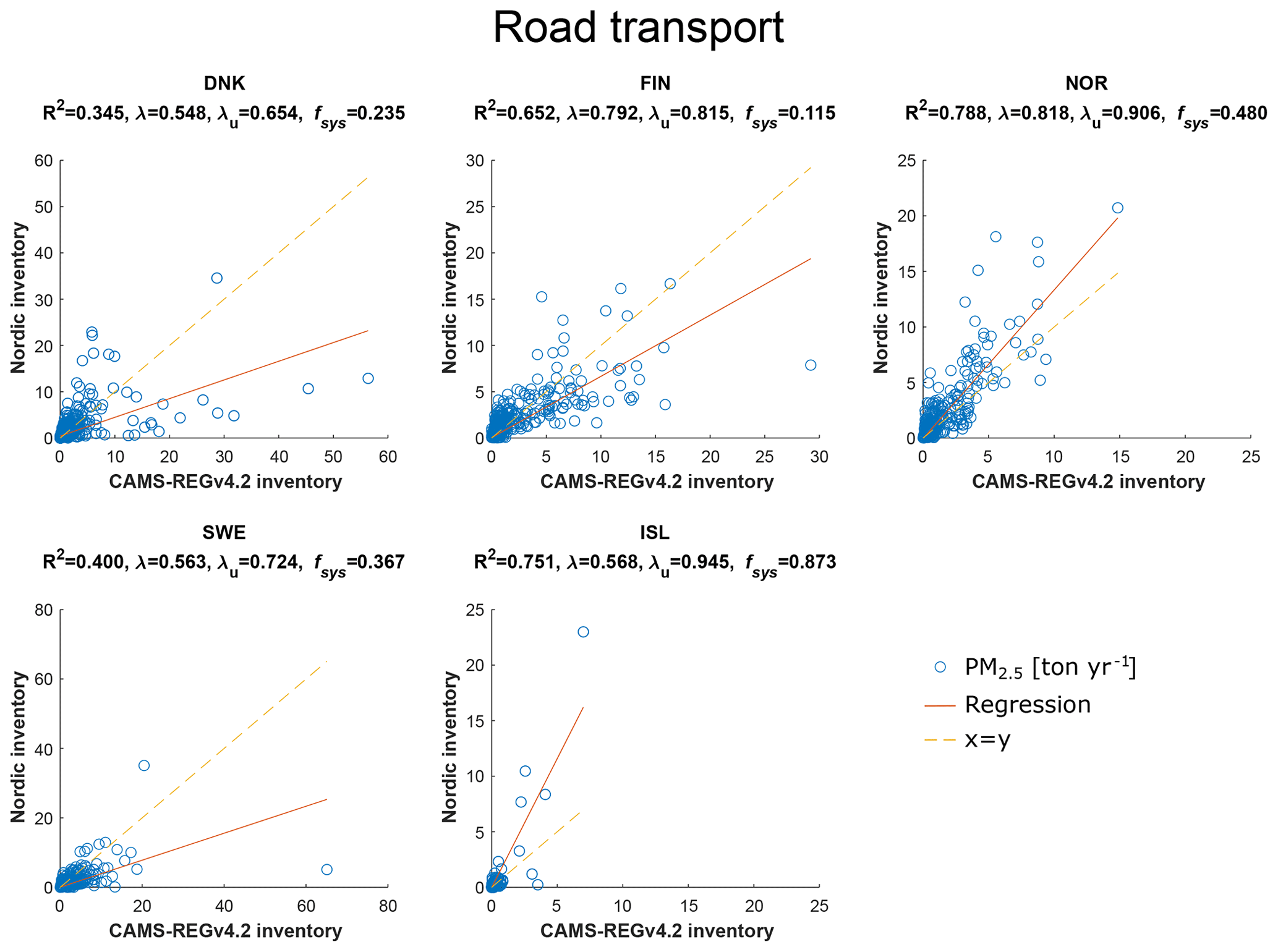
Figure 7 Scatter plots and index of agreement results for road transport sector between our Nordic inventory and the CAMS-REGv4.2 inventory. The circles represent emissions PM_2.5 of a single cell. Orange line is the regression and dashed yellow the y=x line. R² – coefficient of determination, λ – index of agreement, λ_u – unsystematic index, and f_sys – systematic noise.

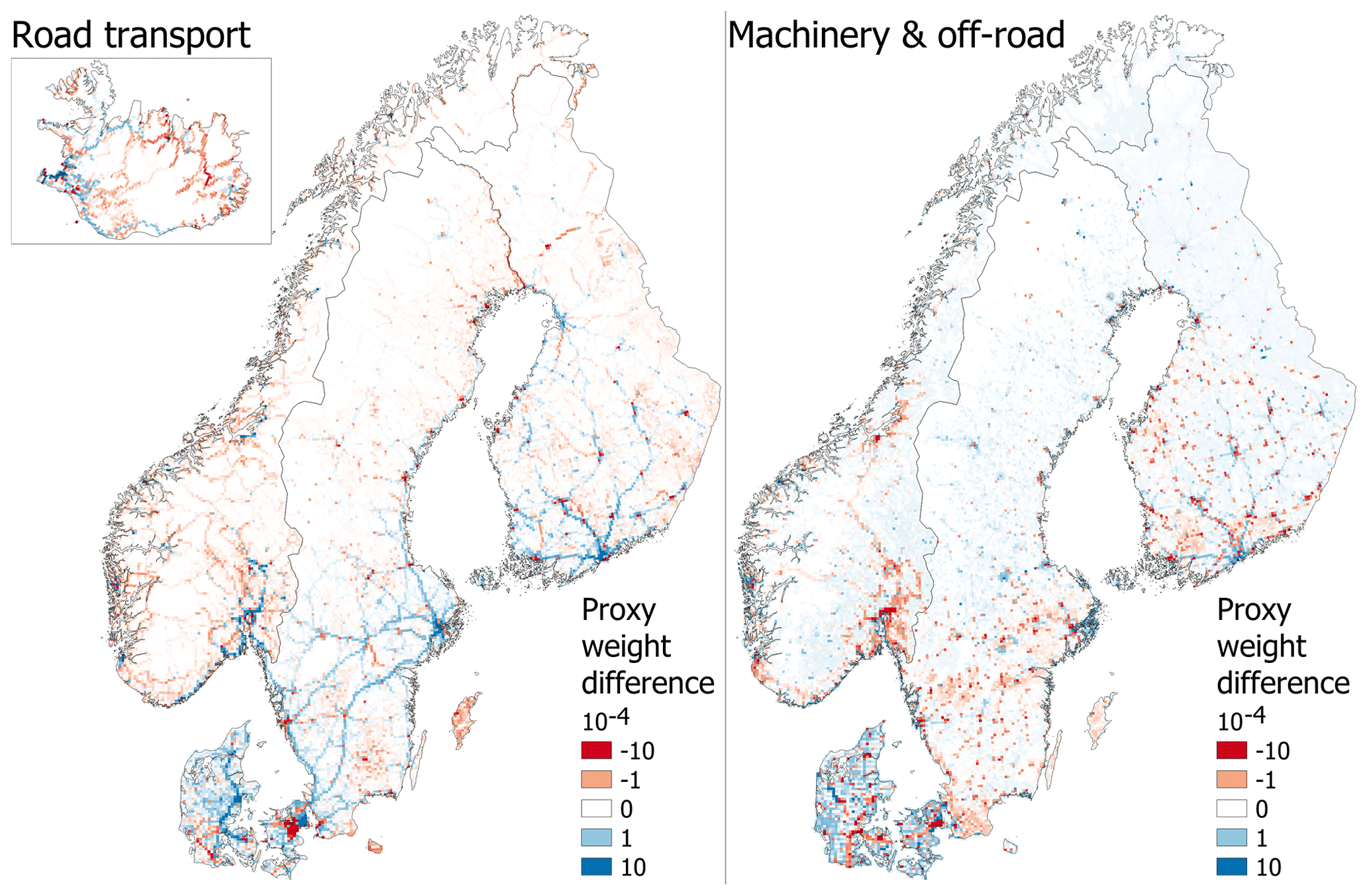
Figure 8 Differences in the PM_2.5 emission proxy weights between the Nordic and CAMS-REGv4.2 inventories. Positive (blue) values indicate cells where the Nordic inventory had higher weight and negative (red) values where the CAMS-REGv4.2 inventory did. The weights have been normalized separately within each country. The legend shows the colours at the exact values, and colours between these values are interpolated.

For machinery, the index of agreement results were poor for Denmark and Norway. For Finland and Sweden they were higher, almost as good as the best values for road transport. For Norway, the main reason was the difference in the total emissions, as seen by f_sys, which indicates the portion of systematic difference in the index. If the emissions were similar, the index would be the highest from all the Nordic countries.

In Finland, Norway, and Sweden, both inventories weighted most emissions to cities. The CAMS-REGv4.2 inventory had more weight in most cities, except Helsinki and a few cells in Stockholm. It also had more weight in agriculture land in all countries but Denmark. Outside city centres and agricultural fields, CAMS-REGv4.2 had small emissions. The Nordic inventory had not only more emissions but also more cells with emissions (albeit low) in non-agricultural rural areas. Also, the Nordic inventory had a higher weight on highways and mines in Finland and in a few railroad stations and their surroundings and mines in Sweden. In Denmark, the Nordic inventory had more even distribution with a higher weight in the rural, agricultural areas and on a few highways (due to the construction of them). CAMS-REGv4.2 had a higher weight on main highways and cities, especially in the Copenhagen area. In general, CAMS-REGv4.2 used population as a proxy much more than the Nordic inventory.

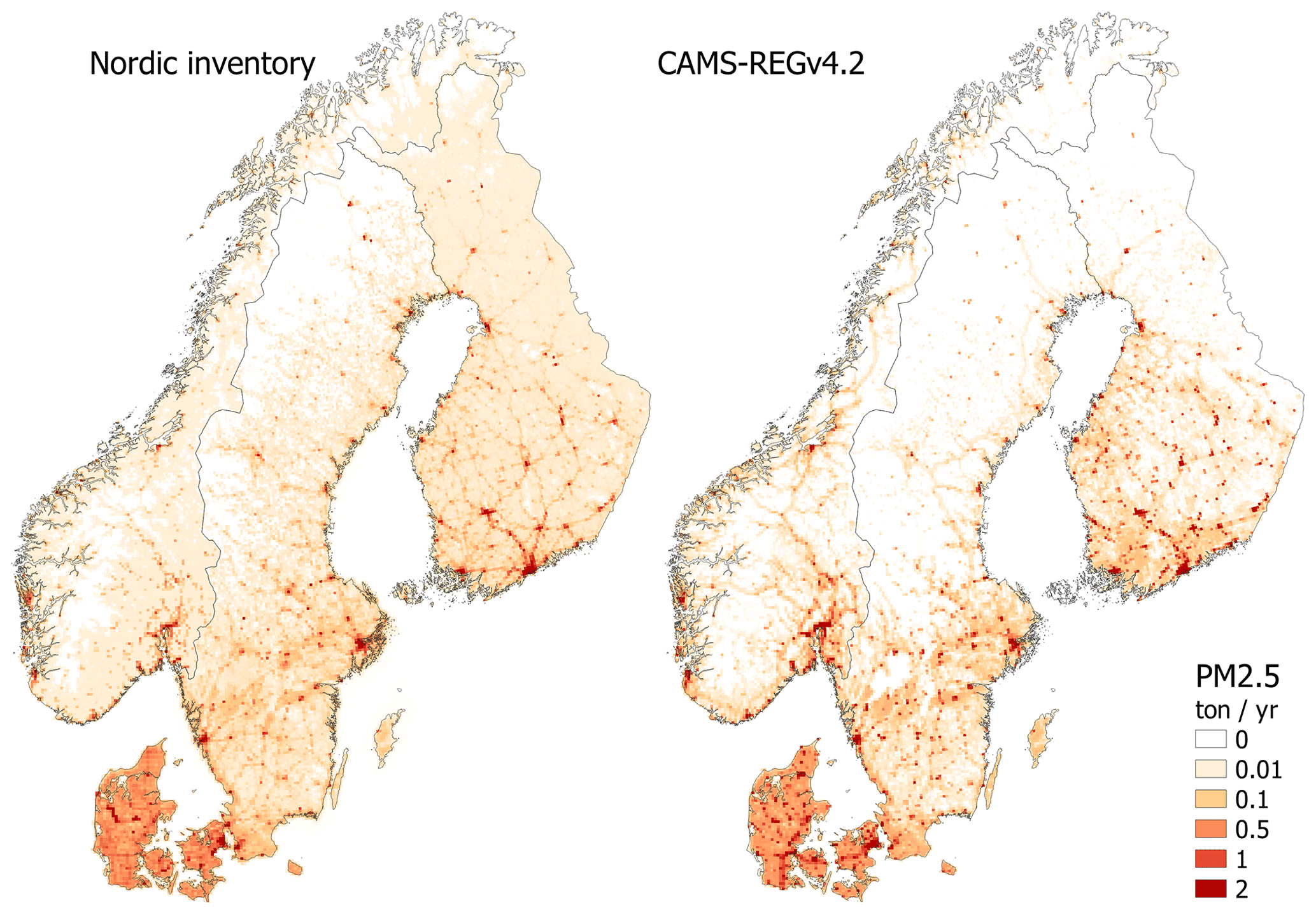
Figure 9 Spatial distribution of machinery and off-road PM_2.5 emissions in the Nordic inventory on the left and CAMS-REGv4.2 on the right. The legend shows the colours at the exact emissions values, and colours between these values are interpolated.

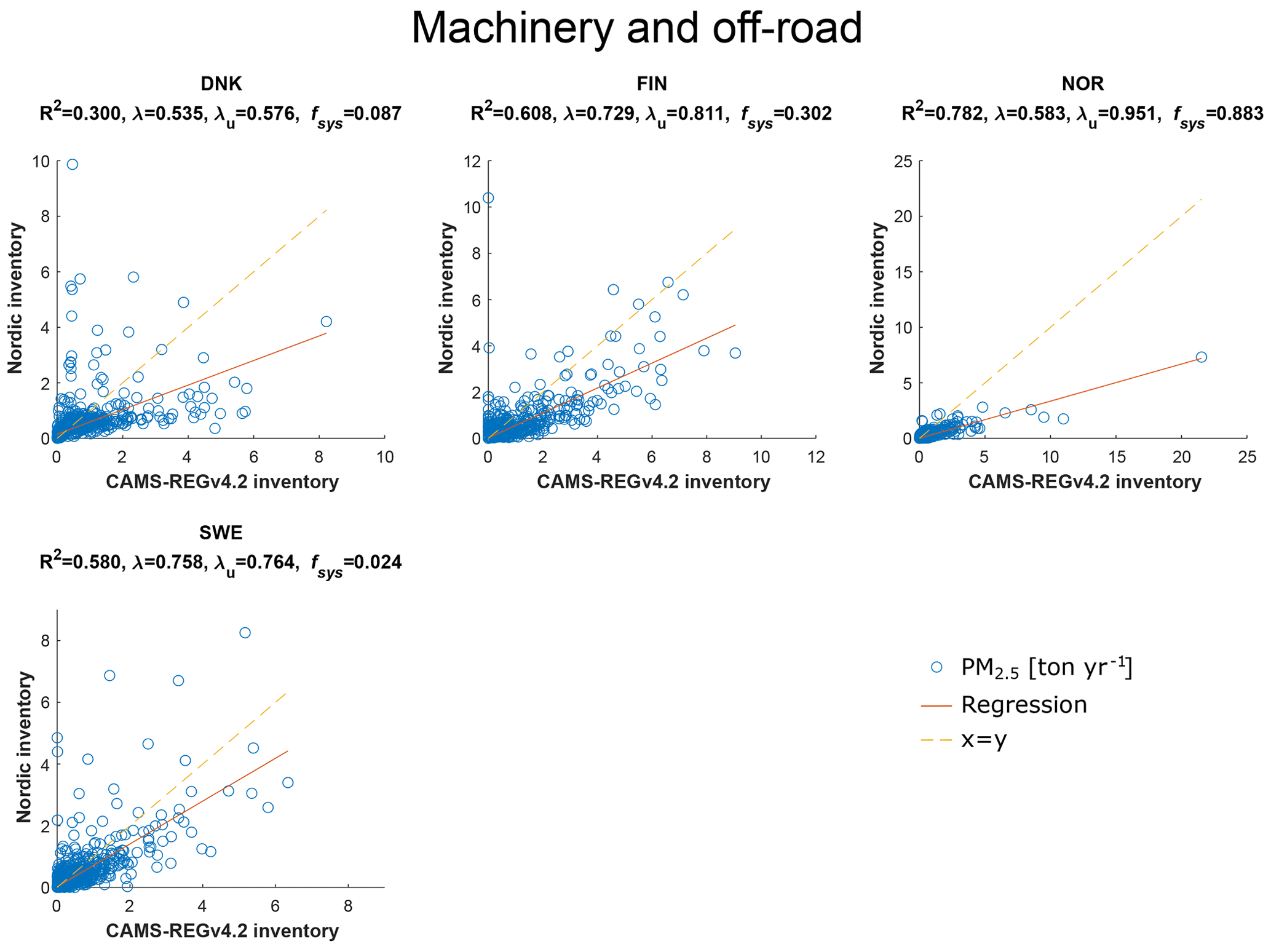
Figure 10 Scatter plots and index of agreement results for the machinery and off-road sector between our Nordic and the CAMS-REGv4.2 inventory. The circles represent PM_2.5 emissions of a single cell. Orange line is the regression and dashed yellow the y=x-line. R²= coefficient of determination, λ – index of agreement, λ_u – unsystematic index, and f_sys – systematic noise.

4 Discussion

Our paper describes how the Nordic countries spatially distribute the air pollution emissions of road transport and machinery and off-road sectors. While we have considered the spatial distributions of PM_2.5 emissions, the conclusions hold for other pollutants as well. This is because the spatial proxies are developed for each (sub)sector, instead of being pollutant specific. Furthermore, we chose PM_2.5 since it causes largest part of adverse health effects from air pollution, and primary PM_2.5 emissions has the greatest impact on local air quality. Therefore, a high resolution and a detailed spatial distribution of emissions are especially important for PM_2.5. In the following we will discuss the similarities and differences in methods and data that can be used to do this.

4.1 Road transport

The EMEP/EEA Guidebook (European Environment Agency, 2019) uses the nomenclature for reporting (NFR) format, which differs somewhat from the SNAP nomenclature used in our Nordic inventory. For road transport, the guidebook recommends traffic flows and types of vehicles as the best-tier spatial proxy. In each country of our Nordic inventory, either measured or estimated traffic flow was used, and vehicle categories were separated at least between heavy- and light-duty transport. Therefore, our inventory complies with the Tier 3 recommendation. The main differences between the countries were the number of vehicle categories (from two in Norway and Sweden to four in Finland) and how many measured traffic flow data were available (and how much modelled traffic was needed to complete the proxies).

The EMEP/EEA Guidebook does not have separate recommendations for traffic dust emissions (brake and tyre wear, road abrasion, resuspension (not required for reporting and not included in the guidebook)). However, due to climate conditions, traffic dust is an important emission category in the Nordic countries. The emissions spike in spring, when snow melts, and (studded) winter tyres wear the road surface, and also, accumulated dust is resuspended into the air. The traffic exhaust and dust emissions were mostly distributed with the same proxies in the Nordic countries, although Finland had separate municipal level proxy for them. However, regional weather conditions, which have strong impact on the dust emissions, could be taken into account within each country. The NORTRIP (NOn-exhaust Road TRaffic Induced Particle) road dust emission model (Denby et al., 2013) contains the effect of weather to the emissions and could be used to create regional weights for dust emissions. It should be noted that Denmark differs from the rest of the Nordics, as its climate resembles central Europe more than the other Nordic countries. This highlights that the spatial weights should be determined regionally within each country with local weather parameters.

The comparison of our Nordic inventory to CAMS-REGv4.2 shows how the combination of locally measured and modelled traffic volume data compares to more general modelled data. Overall, the spatial distribution with the more general data was similar to the more detailed results in the Nordic inventory. It seems that highways were more weighted in the Nordic inventory, suggesting that the traffic modelling used in the Open Transport Map, which CAMS-REG is based on, does not catch the traffic volumes on busy, large roads well enough. Interestingly, CAMS-REG also had lower weight in capital city centres than the Nordic inventory but higher weights in the outskirts of the capitals and smaller cities. An exception was Helsinki, where the CAMS-REGv4.2 inventory had higher weight in the cell covering the city centre. The Nordic inventory weighted more traffic and emissions on the ring roads of the Helsinki metropolitan area. It seems that the Open Transport Map traffic modelling creates activity based on population density and around transport hubs such airports and harbours. However, it does not allocate high traffic activity to the capital cities (except in the centre of Helsinki). All these factors could affect air pollution health impact modelling results, as densely populated areas are most important for exposure modelling results.

4.2 Machinery and off-road

For the machinery and off-road sector, the EMEP/EEA Guidebook includes recommendations within broader sectors. For example, industrial machinery is in the same group as “Stationary combustion in manufacturing industries and construction: Other”. The recommended proxies are often grouped in the same way and not necessarily specific to machinery and off-road activities. It should be noted that we have used higher resolution (1 km × 1 km) than in the official gridded emission data reporting (0.1° × 0.1°) targeted by the guidebook chapter on spatial emissions mapping. The resolution will affect what type of data can represent the activities on the chosen scale.

For industrial and commercial machinery, the guidebook recommends using point source data where possible. For industry, our inventory mainly uses industrial areas from land cover data, which are Tier 1 in the guidebook. We argue that land cover is more suitable than point sources for industrial machinery, as the area where the machinery is used is better covered with such data. Point-source-specific production numbers, for example, could be included in the proxy to weight the emissions between the industrial areas, but to enhance the spatial distribution, this would need information on industry-specific use of the machinery.

Similarly, for agriculture, forestry, and residential machinery sources, we used corresponding land use data, which are Tier 1 in the guidebook. Tier 3 suggests detailed fuel deliveries with employment data for forestry and agriculture and detailed fuel deliveries with population density and/or household numbers and types for residential. Fuel deliveries could possibly be found on, for example, a regional level, possibly enhancing the spatial distribution between regions. Increasing the detail beyond land use on forestry and agriculture is difficult. From an air quality point of view, these sources are not the most important, as, especially in the Nordic countries, the activities mostly take place far away from population centres (with possible exception the more densely populated Denmark). Therefore, the land use as a proxy is sufficient to get the emissions away from cities.

Roads were used very differently in the countries as a proxy for machinery. Finland weighted them most, allocating road maintenance to them, while Norway did not use road information for machinery. Denmark had much weight on the roads like Finland but also had high emissions on a few highways due to their construction. This highlights the differences in the spatial distribution methods between the Nordic countries and how there is still room for development and learning from each other.

In the machinery and off-road sector, the CAMS-REGv4.2 inventory's spatial distribution was mainly driven by population and secondarily by agriculture land. In the Nordic inventory, only Finland used population as proxy data and only for part of the other machinery subsector. Furthermore, the Nordic inventory utilized the variety of other proxy data more than the CAMS-REGv4.2 inventory, distributing more emissions to other areas than city centres and fields. Despite the different weighting, most emissions were in same areas in all countries, except Denmark, in the two inventories. Therefore, the main characteristics of the sector were captured on the spatial resolution that the CAMS-REGv4.2 inventory had. With the Nordic inventory's higher spatial resolution, more details can be seen within the high emission areas, which would impact health impact assessment results.

4.3 Other factors relating to spatial distribution

While the countries use the same sector nomenclature, subsectors for which the proxies have been applied are not necessarily the same. In particular, the machinery and off-road sector can be divided into different subsectors, depending on the data available for activity and suitable proxies. For example, emissions can be calculated for excavators and those emissions divided to several subsectors such as construction and industry, with specific proxies. But this is only one way to do the aggregation, and available proxies dictate the possibilities.

The impact of resolution on exposure assessment has been presented in Korhonen et al. (2019). They found that for Finland, going from 5 to 1 km in assessment resolution had a significant impact on the exposure results in urban areas. For road transport and machinery, the lower resolution of 5 km in the exposure modelling led to a mortality estimate about 25 %–30 % smaller in urban areas compared to the 1 km resolution. A decrease from 1 to 10 km resolution caused a mortality estimate that was over 40 % smaller. In rural areas the same resolution changes from 1 to 5 km and from 1 to 10 km caused a 10 % and 20 % drop in the mortality estimate, respectively. Therefore, even though the Nordic and CAMS-REGv4.2 inventories give similar results on CAMS-REGv4.2's resolution (5.5 km × 3.5–6.5 km, with the north–south length being shorter in north), the Nordic inventory allows more detailed health impact assessments with its higher resolution.

One aspect to consider regarding the time series of the Nordic inventory is that Finland and Norway have unchanging proxies between the years; i.e. the same spatial distribution is used for all years for a specific subsector. In Denmark some proxies are updated annually, and subsectors can have year-specific proxies. Sweden does the same for proxies for national to municipal/county level. Year-specific proxies can reduce the uncertainty of the spatial distribution, but they are also dependent on appropriate data. The spatial distributions do not necessarily change drastically from year to year, making static proxies more justified. However, as our inventory spans 1990 to 2014, it is reasonable to assume that there have been changes which would affect the results in significant way. Furthermore, although beyond the scope of our inventory in this paper, the COVID pandemic clearly has affected the activities of people, meaning more attention needs to be given to dynamic proxies, as has been reported in Guevara et al. (2022).

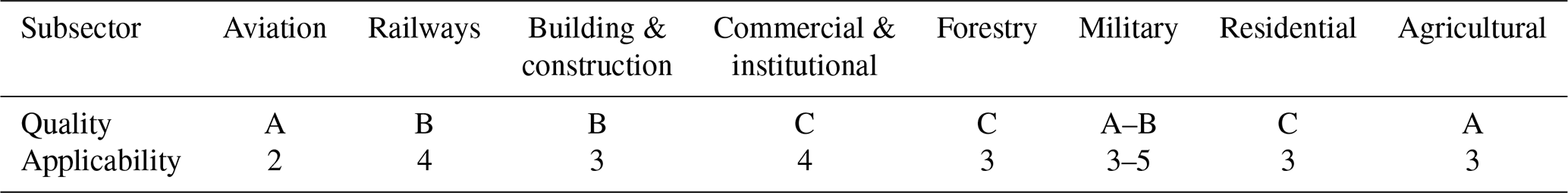
Uncertainties associated with the proxies were not analysed in this work. Some assessments have previously been made. Plejdrup et al. (2021) describe the assessed quality of a dataset (A to E, A being the highest) and applicability as a proxy (1–5, 1 being the highest) for proxies used in Denmark, both with a five-step classification. For road transport, they assess their proxies as low uncertainty in the dataset (B; second-best certainty class) and as “Good correlated proxy” (2; second-best applicability class), as a vast amount of traffic data is used for the proxy. For the machinery and off-road sector, the assessed ratings are presented in Table 7. In general, the quality of the datasets is considered to be better than the applicability. The main problem in applicability is thought to be a lack of spatial activity data to accompany other, for example, land use, data. Therefore, according to the report, the datasets used for proxy development have medium to low uncertainty, and the main development need is finding appropriate data to describe the activities spatially within the identified areas, for example, land use classes.

Table 7 Assessed quality of dataset used and its applicability as a proxy for machinery and off-road sector proxies in Denmark (Plejdrup et al., 2021). Quality ranges from A–E (A being the highest) and applicability from 1–5 (1 being the highest).

The Nordic emission inventory has been used as input to the coupled DEHM/UBM air pollution model system setup for the continental Nordic area within the same spatial 1 km × 1 km grid. A decades-long simulation has been evaluated against observations representing both rural and urban conditions, showing that the model capture the main features in terms of spatial–temporal variability of air pollution across the Nordic (Frohn et al., 2022); the annual, country-level correlation coefficients were in the range from 0.7–0.9 for NO₂, 0.6–0.7 for O₃, and 0.4–0.9 for PM_2.5. This simulation has also been used for a study comparing different health assessment tools (Lehtomäki et al., 2020) and for several health studies based on detailed Nordic health data. The studies confirm that even low levels of air pollution can be associated with negative impacts on human health (Olsson et al., 2021; Raaschou-Nielsen et al., 2023; Sommar et al., 2021).

5 Data availability

The Nordic emission inventory (Paunu et al., 2023) is published as open-source data on Zenodo and can be accessed at https://doi.org/10.5281/zenodo.10571094.

6 Conclusions

In this paper we have presented our novel Nordic air pollution emission inventory and described how spatial distribution of road transport and machinery and off-road mobile source emissions is affected by the choice of proxy data. Our inventory contains annual air pollution emissions at a high spatial resolution (1 km × 1 km) from 1990–2014. The inventory is published as open-source data to be freely used in, for example, impact assessments (Paunu et al., 2023).

For road transport, all countries in our Nordic inventory complied with the Tier 3 recommendation of the EMEP/EEA Guidebook on spatial distribution of the emissions. There were different ways to categorize vehicle classes, and more detailed division could be applied in the countries, but most important was the distinction between heavy- and light-duty vehicles. Improvement possibilities were in replacing modelled traffic volume data with measured data where possible. Furthermore, traffic dust emissions did not have distinct proxies. Regional proxies, which would consider local (especially winter and spring) weather conditions, would be possible to develop and apply within each country. The issue is most relevant in northern Europe, and, therefore, a general EMEP/EEA Guidebook update might not be needed.

Comparison to the European-wide CAMS-REGv4.2 inventory showed that their proxy, based more on modelled traffic volumes, compared to the proxy in the Nordic inventory, based on a mix of locally measured and modelled traffic volumes, created lower emission weights on highways and capitals and higher weights in other cities and population centres. In other words, modelled traffic volumes based on population did not catch the extent of traffic on larger roads. This would have impact on population exposure and health impact assessments, as emissions close to population will increase the estimated impacts. Therefore, more attention should be focused on traffic volume modelling to improve the spatial proxies for road transport.

The proxies for machinery and off-road emissions in our Nordic inventory differed from the Tier 3 recommendations in the EMEP/EEA Guidebook. The guidebook recommendations for the machinery and off-road sector are included within broader sectors and suggest that point source and fuel delivery data are used. For many subsectors, our Nordic inventory utilizes land use data, which are Tier 1 (most simple tier) in the guidebook. However, we argue that for many machinery and off-road activities, the land use data are the best available starting point for the proxies, as explained in the Discussion section. From a health impact assessment point of view, for many emission sectors, such as agriculture and forestry, the main issue is to distribute the emissions away from population centres, which is easily achieved with suitable land use classes. The distribution can be enhanced using available data related to the activity, such as regional tractor distribution or annual loggings, or the suggested fuel deliveries. Our Nordic inventory could be developed further by including year-specific spatial proxies for Finland and Norway, as Denmark and Sweden have already done.

CAMS-REGv4.2, despite having less complex proxies for machinery and off-road, was able to produce similar spatial patterns for the emissions to our Nordic inventory in three of the four countries. The conclusion holds for the resolution of the CAMS-REGv4.2 inventory. Our Nordic inventory has higher native resolution (1 km × 1 km vs. 0.1° × 0.05° of CAMS-REGv4.2) and offers more details in the spatial pattern. This is especially important in cities, where both population density and emissions are highest. Therefore, the Nordic inventory allows for more detailed health impact assessments.

We suggest that the EMEP/EEA Guidebook should have separate recommendations for the machinery and off-road proxies instead of including them within more broad sector division. Furthermore, measured traffic flows should be utilized where possible in lieu of modelled data. Land use data are a good starting point for a proxy and can, with success, be combined with other activity-specific data to enhance the quality of the spatial distribution.