GLC_FCS30D: the first global 30 m land-cover dynamics monitoring product with a fine classification system for the period from 1985 to 2022 generated using dense-time-series Landsat imagery and the continuous change-detection method

Land-cover change has been identified as an important cause or driving force of global climate change and is a significant research topic. Over the past few decades, global land-cover mapping has progressed; however, long-time-series global land-cover-change monitoring data are still sparse, especially those at 30 m resolution. In this study, we describe GLC_FCS30D, a novel global 30 m land-cover dynamics monitoring dataset containing 35 land-cover subcategories and covering the period 1985–2022 in 26 time steps (maps were updated every 5 years before 2000 and annually after 2000). GLC_FCS30D has been developed using continuous change detection and all available Landsat imagery based on the Google Earth Engine platform. Specifically, we first take advantage of the continuous change-detection model and the full time series of Landsat observations to capture the time points of changed pixels and identify the temporally stable areas. Then, we apply a spatiotemporal refinement method to derive the globally distributed and high-confidence training samples from these temporally stable areas. Next, local adaptive classification models are used to update the land-cover information for the changed pixels, and a temporal-consistency optimization algorithm is adopted to improve their temporal stability and suppress some false changes. Further, the GLC_FCS30D product is validated using 84 526 globally distributed validation samples from 2020. It achieves an overall accuracy of 80.88 % (±0.27 %) for the basic classification system (10 major land-cover types) and 73.04 % (±0.30 %) for the LCCS (Land Cover Classification System) level-1 validation system (17 LCCS land-cover types). Meanwhile, two third-party time-series datasets used for validation from the United States and Europe Union are also collected for analyzing accuracy variations, and the results show that GLC_FCS30D offers significant stability in terms of variation across the accuracy time series and achieves mean accuracies of 79.50 % (±0.50 %) and 81.91 % (±0.09 %) over the two regions. Lastly, we draw conclusions about the global land-cover-change information from the GLC_FCS30D dataset; namely, that forest and cropland variations have dominated global land-cover change over past 37 years, the net loss of forests reached about 2.5 million km², and the net gain in cropland area is approximately 1.3 million km². Therefore, the novel dataset GLC_FCS30D is an accurate land-cover-dynamics time-series monitoring product that benefits from its diverse classification system, high spatial resolution, and long time span (1985–2022); thus, it will effectively support global climate change research and promote sustainable development analysis. The GLC_FCS30D dataset is available via https://doi.org/10.5281/zenodo.8239305 (Liu et al., 2023).

1 Introduction

Land-cover data are important and necessary for supporting sustainable development goals, maintaining biodiversity, and monitoring natural resources (L. Liu et al., 2021; Potapov et al., 2022). Land-cover changes directly or indirectly influence global climate patterns and the speed and magnitude of climate change (Song et al., 2018), and they increasingly affect biogeochemical cycles, the carbon cycle, and the Earth's energy balance (Foley et al., 2005; Hong et al., 2021; Winkler et al., 2021). Since the Industrial Revolution, under the dual pressure from global climate change and human activities, global land cover has undergone drastic changes. According to a Global Carbon Project report in 2020, since the industrialization period, land-cover and land-use changes have contributed to approximately 25 % of all global greenhouse gas emissions (Friedlingstein et al., 2020), and this trend is exacerbated by the ongoing increase in population and per capita energy consumption (Xian et al., 2022). Therefore, understanding and studying land-cover changes is of vital significance for addressing global environmental changes, promoting sustainable development, and safeguarding the Earth's ecological environment.

Remote-sensing techniques, with their periodic Earth observation capability and archived massive long-term observation data since 1972, provide the most cost-effective and practical solutions for long-time-series, large-area land-cover-change monitoring. In the past few decades, with the continuous improvement of remote sensing technology and storage and computing capabilities, global land-cover-change monitoring (GLCCM) has transitioned from 1 km spatial resolution to fine resolutions of 30 or 10 m and from single-phase mapping to long-term monitoring (Ban et al., 2015; Friedl et al., 2010, 2022; Giri et al., 2013). In its early stages, GLCCM mainly relied on time series of MODIS, AVHRR, and Project for Onboard Autonomy (PROBA)-V imagery (Buchhorn et al., 2020; Friedl et al., 2010); for example, Sulla-Menashe et al. (2019) generated a global 500 m annual land-cover product (MCD12Q1) covering the period from 2001 to the present using MODIS time-series imagery with an overall accuracy of 73.6 %. Defourny et al. (2018) integrated PROBA-V and Medium Resolution Imaging Spectrometer (MERIS) time-series observations to develop a global 300 m annual land-cover dynamics dataset (CCI_LC: Climate Change Initiative Global Land Cover) for the period from 1992 to 2020 with an overall accuracy of 71.5 %. These coarse land-cover-change products comprehensively captured the spatial patterns of various land-cover types and quantified the global land-cover changes caused by human and natural activities. However, they still had major limitations, especially in regions with intense human activity and high spatial heterogeneity, because these broken and heterogeneous land-cover changes cannot be captured by coarse-resolution satellite observations (Hansen et al., 2013; Herold et al., 2008; L. Liu et al., 2021; Y. Zhang et al., 2021).

Recently, benefiting from the free access to fine-resolution satellite imagery and powerful computing and storage capabilities and the rise of cloud computing (such as the Google Earth Engine (Gorelick et al., 2017) and Microsoft Planetary Computer) in particular, fine-resolution land-cover dynamics monitoring has been experiencing rapid development. Correspondingly, numerous national and global 30 m land-cover dynamics products have been developed (Chen et al., 2015; Homer et al., 2020; H. Liu et al., 2021; Potapov et al., 2022; Yang and Huang, 2021; Zhang et al., 2022). For example, Yang and Huang (2021) used China's land-use/cover datasets (CLUDs) as the prior dataset and then combined multitemporal classification and spatiotemporal consistency post-processing methods to develop an annual 30 m land-cover dataset (CLCD) for China from 1990 to 2019. Similarly, H. Liu et al. (2021) combined pixel-based classification and spatiotemporal consistency post-processing methods to generate the first global 30 m land-cover change products. However, many studies have demonstrated that multiperiod independent classifications lead to significant classification error accumulation in land-cover-change time-series monitoring (Sulla-Menashe et al., 2019; Zhu, 2017). For example, Xian et al. (2022) stated that the independent classification strategy suffered from the constraints of the post-processing requirements that ensure the temporal consistency of land-cover change maps. Therefore, although GLCCM has progressed significantly over the past few decades, an accurate global 30 m land-cover change-detection product generated by an efficient land-cover change method is still urgently required.

One of the greatest challenges in large-area land-cover change detection is to select the optimal algorithm to capture the land-cover changes from time-series observations (Healey et al., 2018; Zhu, 2017). Over the past few decades, a series of change-detection algorithms have been proposed for monitoring forest disturbance (Huang et al., 2009; Jin et al., 2023; Kennedy et al., 2007, 2010; Qin et al., 2021), urban expansion (Liu et al., 2019; X. Zhang et al., 2021a), cropland dynamics (Dong et al., 2015; Potapov et al., 2021), and land-cover changes (Bullock et al., 2019; Jin et al., 2017; Verbesselt et al., 2010; Zhu et al., 2019). However, most of them are only suitable for regional land-cover change monitoring, and some of the algorithms need prior knowledge (such as that for urban expansion). Zhu (2017) systematically reviewed the performance and limitations of various change-detection methods based on multitemporal satellite data and further explained that the high-temporal-frequency and multivariate change-detection algorithms are more suitable for a long time series of land-cover changes in a large area, provided that the problem of the huge amount of computation involved can be solved. Similarly, Xian et al. (2022) and Liu et al. (2019) concluded that dense and continuous change-detection methods provided higher accuracy and more robustness than traditional change-detection methods for capturing multiple, complicated changes.

The continuous change-detection and classification (CCDC) algorithm, a classical change-detection method based on dense time-series observations proposed by Zhu and Woodcock (2014b), is widely used for regional and national land-cover monitoring (Xian et al., 2022; Xie et al., 2022). It uses all available Landsat observations to build time-series regression models and then captures the outliers by analyzing the differences between the actual observations and model estimations. Zhu and Woodcock (2014b) demonstrated that the CCDC algorithm attained a general accuracy of 90 % and temporal accuracy of 80 % for capturing land-cover changes. Thus, it has been adopted by the United States Geological Survey (USGS) as the official algorithm for monitoring land-cover changes over the United States (Pengra et al., 2016). For example, Xian et al. (2022) implemented the CCDC algorithm and all available Landsat data to develop annual land-cover-change products that cover the contiguous United States (CONUS) for 1985–2017 with an overall accuracy of 82.5 %.

In summary, in recent decades, land-cover mapping and monitoring has made significant progress; however, global 30 m land-cover-dynamics time-series products derived from change-detection algorithms are still lacking. In this study, we had three aims: (1) to use the continuous change-detection algorithm and the full time series of Landsat observations to generate the first global 30 m land-cover dynamics product that covers the period from 1985 to 2022 and uses a fine classification system that contains 35 fine land-cover subcategories with 26 time steps (the maps are updated every 5 years before 2000 and annually after 2000), known as GLC_FCS30D (it should be noted that GLC_FCS30D is updated every 5 years before 2000 due to the sparse availability of Landsat 5 imagery; thus, we combine the satellite observations from 2 years before and after the nominal center year from 1985 to 1995 to ensure the mapping accuracy of GLC_FCS30D before 2000); (2) to quantify the land-cover changes and analyze the spatiotemporal change patterns of various land-cover types based on the developed GLC_FCS30D dataset; and (3) to quantitatively analyze the performance of the GLC_FCS30D product using multisourced validation datasets.

2 Datasets

2.1 Continuous Landsat imagery from 1984 to 2022

All available Landsat imagery from 1984 to 2022 – covering the Landsat 5 Thematic Mapper (TM), Landsat 7 Enhanced Thematic Mapper Plus (ETM+), Landsat 8 Operational Land Imager (OLI), and Landsat 9 OLI missions – were collected via the Google Earth Engine (GEE) cloud-computing platform. Specific measures were taken to build a high-quality, continuous Landsat time-series collection. First, all Landsat images underwent atmospheric correction to convert them to surface reflectance using the Landsat Ecosystem Disturbance Adaptive Processing System (LEDAPS) and Land Surface Reflectance Code (LaSRC) methods (Vermote, 2007; Vermote and Kotchenova, 2008). Then, although the Landsat 5, 7, 8, and 9 missions share similar spectral bands, the wavelength differences between the TM, ETM+, and OLI cannot be ignored. Relative radiometric normalization was applied to the TM and ETM+ imagery using the transformation coefficients suggested by Roy et al. (2016).

2.2 Global land-cover dataset at 30 m for the year 2020

The global 30 m land-cover product with a fine classification system for the year 2020 (GLC_FCS30-2020) is the baseline for generating training samples and identifying land-cover information in the temporally stable regions in Sect. 3. The GLC_FCS30 dataset was developed using local adaptive classifications and confident and globally distributed training samples, and then validated to reach an overall accuracy of 82.5 % with the basic validation system (X. Zhang et al., 2021b). Cross-comparisons with other land-cover products showed obvious advantages for GLC_FCS30 in terms of mapping accuracy and diversity of land-cover types. The GLC_FCS30-2020 dataset is freely available at https://doi.org/10.5281/zenodo.4280923 (Liu et al., 2020).

2.3 Global impervious surface dynamics dataset at 30 m from 1985 to 2022

Many studies found that high spatiotemporal heterogeneity of impervious surfaces and broken impervious surface constructions caused high uncertainty and difficulty when monitoring the dynamics of such surfaces (Gong et al., 2019a; Zhang et al., 2022), and issues with both missed detections and false alarms are encountered when change detection methods are applied to the dynamic monitoring of heterogeneous impervious surfaces. Thus, we independently produced a global impervious-surface-dynamics time-series dataset at 30 m (GISD30) for 1985–2022 and then overlaid this thematic dataset on the GLC_FCS30D dataset to ensure high confidence in the impervious surface dynamics. The GISD30 dataset was developed by combining the sample migration, spectral generalization, and local adaptive modeling methods and then optimized by the spatiotemporal-consistency correction method (Zhang et al., 2022). It was validated and found to attain a mean overall accuracy of 90.1 % around the globe and to perform better than other similar products in capturing the changes in impervious surfaces over time and across different types of landscapes. At the same time, third-party validation also indicated that GISD30 exhibited superior performance to similar global 30 m impervious surface products (Wang et al., 2022).

2.4 Global 30 m wetland datasets from 1985 to 2022

Like the impervious surface dataset, the global wetland dynamics dataset is independently produced because the reflectance spectra of the wetlands and phenological variations changed daily with the water levels. The continuous change-detection method would suffer from serious commission and omission errors if used for wetland dynamics monitoring (Gallant, 2015). In this study, the GWL_FCS30 (global 30 m wetland map with a fine classification system) wetland dataset from 1985 to 2022 – developed by integrating the automatic sample extraction method, a stratified classification strategy, and the time series of Landsat observations (Zhang et al., 2023) – is superimposed on the GLC_FCS30D land-cover dynamics dataset. GWL_FCS30 was quantitatively assessed as having a mean overall accuracy of 86.44 % using 25 708 validation points, and it demonstrated a higher level of performance than other wetland products when it came to capturing the spatial patterns of wetlands during cross-comparisons (Zhang et al., 2023). GWL_FCS30 further splits wetlands into seven wetland subcategories (four inland and three coastal subcategories) and is overlaid directly onto the GLC_FCS30D dataset to not only improve the monitoring accuracy for wetlands but also enrich the number of land-cover types (see Table 1).

2.5 Validation datasets

To comprehensively analyze the accuracy metrics for the GLC_FCS30D dataset, two types of validation datasets were collected: an independent global validation dataset from 2020 and two third-party time-series datasets used for validation for the United States and the European Union.

2.5.1 Global validation dataset

A total of 84 526 globally distributed validation samples are collected to analyze the accuracy metrics for the GLC_FCS30D dataset for 2020, and their spatial distribution is illustrated in Fig. 1. Intuitively, the spatial patterns of the global validation dataset are consistent with the actual global land-cover situation. Specifically, to ensure confidence in and the rationality of the validation datasets, several measures are taken, which were explained in detail in our previous work (Zhao et al., 2023). First, a stratified random sampling method is applied by combining the landscape heterogeneity, population density data, and Köppen climate groups, which effectively increases the sample size in the heterogeneous landscapes and for some rare land-cover types (such as impervious surfaces, permanent ice, and snow). Second, for each validation sample, the land-cover type is determined through independent interpretation by trained interpreters after combining high-resolution aerial photography, multitemporal Landsat images, and other relevant ancillary datasets (such as vegetation coverage, tree height, phenological curves, and terrain characteristics). Independent interpretation software based on the GEE platform (https://eliza-ting.users.earthengine.app/view/crd-vit, last access: 12 March 2024) for efficiently recognizing the land-cover types of each sample was also developed. Third, a quality-control operation based on duplicate interpretations is used to ensure the confidence level of each validation sample. Each sample is independently labeled by three junior interpreters and then double-checked by the senior experts, and validation samples with huge disparities are discarded. In addition, because the impervious-surface and wetland datasets were produced independently and were validated in our previous works (Zhang et al., 2023, 2022), the corresponding high-quality validation samples of these two thematic types are also imported into the global validation datasets.

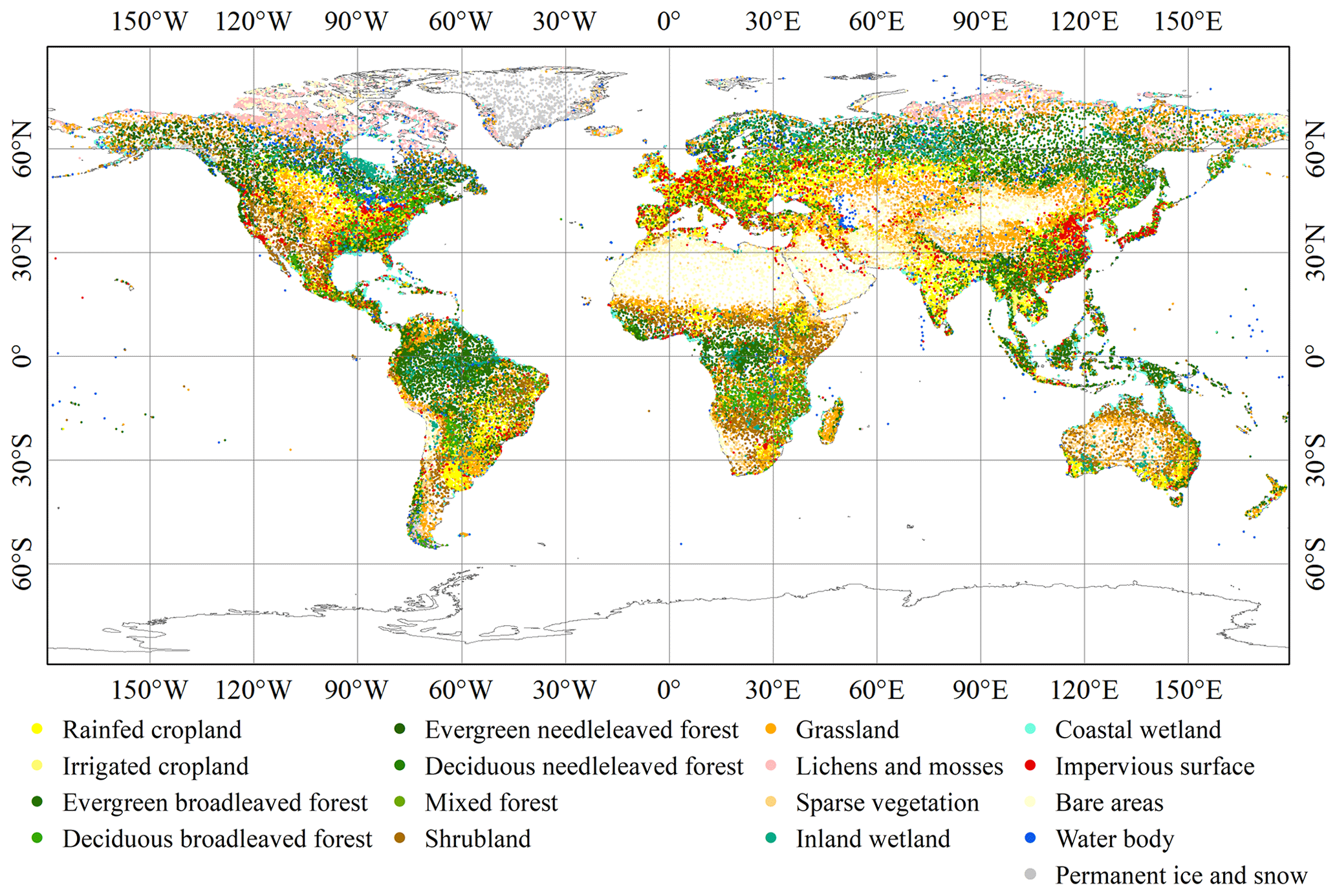
Figure 1 Spatial distribution of 84 526 global validation points relating to 17 fine land-cover types in the normal year of 2020.

2.5.2 Third-party regional time-series datasets used for validation

Due to the great difficulty in collecting global long time-series datasets used for validation, we used two third-party regional datasets for the CONUS and the European Union. The first time-series validation dataset assessed the performance of the Land Cover Monitoring, Assessment, and Projection (LCMAP) Collection 1.0 annual land-cover products (Stehman et al., 2021) (called LCMAP_Val, https://www.usgs.gov/special-topics/lcmap/validation-data, last access: 12 March 2024). LCMAP_Val consisted of 24 971 validation samples with 30 m spatial resolution and covered the time period of 1985 to 2017. It was developed by combining a simple random sampling method and visual interpretation from high-resolution aerial photography, multitemporal Landsat images, and other auxiliary datasets. Meanwhile, to guarantee the reliability of each validation sample, the TimeSync auxiliary tool was also adopted to capture the land-cover changes (Stehman et al., 2021). Quality control was implemented through duplicate interpretations (Xian et al., 2022).

The second regional validation dataset was the Land Use/Cover Area frame Survey (LUCAS), which is the most comprehensive and largest land-cover validation dataset for the European Union and is freely available at https://esdac.jrc.ec.europa.eu/projects/lucas (last access: 12 March 2024). It contains 1 090 863 validation points based on a systematic 2 km × 2 km grid and covers the period from 2006 to 2018 in intervals of 3 years (d'Andrimont et al., 2020). Five LUCAS surveys in 2006, 2009, 2012, 2015, and 2018 assessed the accuracies of the time series of GLC_FCS30D. LUCAS was developed from a combination of field observations and photo interpretation (Ballin et al., 2018); thus, it can be used with high confidence and also attracts widespread attention for land-cover validations (Gao et al., 2020; Venter et al., 2022).

3 Methods

Figure 2 presents a detailed flowchart for monitoring land-cover changes by combining the continuous change-detection (CCD) algorithm proposed by Zhu and Woodcock (2014b) with the local adaptive updating method. Specifically, the flowchart contains four main procedures: (1) detecting the temporally stable pixels and the time points of abrupt changes in the other land-cover pixels using the continuous change-detection model; (2) deriving the spatiotemporally stable training samples by using the spatiotemporal refinement method from the GLC_FCS30 land-cover product and temporally stable masks; (3) building the local adaptive classification models for each local region and then updating the land-cover information in the changed pixels; and (4) using the spatiotemporal consistency optimization method to improve the quality of land-cover change maps and suppress false changes.

Before detecting the changed land-cover pixels, all poor-quality pixels (cloud, shadow, and saturated pixels as well as the “scan line corrector off” pixels in Landsat 7) in the continuous-time-series Landsat imagery were first masked using the CFmask algorithm, which has been demonstrated to achieve an overall accuracy of 96.4 % and was adopted by the USGS as its official cloud and shadow detection algorithm (Zhu et al., 2015; Zhu and Woodcock, 2012). Then, in terms of these residual cloud pixels (i.e., those contaminated with light cloud and haze), the Tmask (multiTemporal mask) algorithm, which uses the temporal information from the clear-sky pixels to improve the cloud-detection capability (Zhu and Woodcock, 2014a), was used to mask the residual cloud pixels (note that Tmask is integrated into the CCD algorithm on the GEE platform as ee.Algorithms.TemporalSegmentation.Ccdc()). In other words, the effect of poor-quality pixels was minimized.

Figure 2 The flowchart of the proposed method combining the continuous change-detection (CCD) algorithm and a local adaptive updating algorithm.

3.1 The fine classification system used in GLC_FCS30D

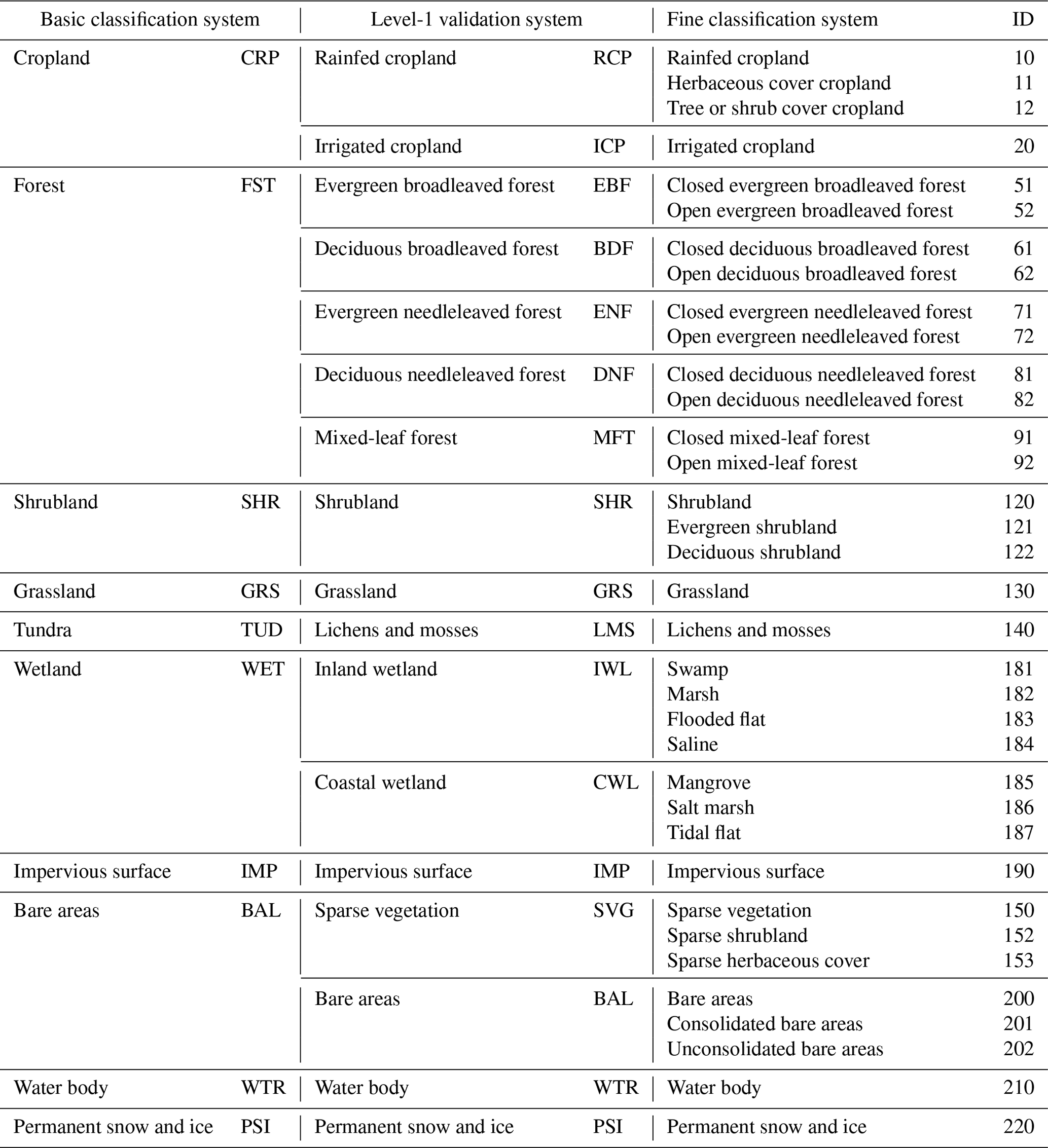
Determining the classification system is usually a prerequisite for land-cover mapping and monitoring. In this study, as we used GLC_FCS30-2020 as the baseline land-cover product and overlaid the GWL_FCS30 dataset on GLC_FCS30D to ensure high accuracy in the wetland areas, the fine classification system used in this study is inherited from those of GLC_FCS30-2020 and GWL_FCS30. Table 1 lists the details of the fine classification system. It contains 35 fine land-cover types and has obvious advantages when identifying forest and wetland subcategories.

Table 1 The details of the fine classification system used in the GLC_FCS30D land-cover dynamics dataset.

3.2 Detecting changes using the CCD algorithm and continuous Landsat imagery

In general, land-cover changes can be grouped into three categories: periodic changes caused by phenological variability, trend changes driven by natural behavior (such as vegetation growth), and abrupt changes caused by natural or human disturbances (such as deforestation or urban expansion). Thus, capturing these abrupt changes and simultaneously suppressing the periodic and trend changes is the key to land-cover monitoring. In this study, the CCD algorithm (Zhu and Woodcock, 2014b) was used to capture these abrupt changes. This algorithm uses Fourier transformation to fit the time-series observations with the trend term (estimating the trend changes) and harmonic terms (describing the periodic changes) in Eq. (1):

$$\begin{array}{}\text{(1)}& \begin{array}{rl}\widehat{\mathit{\rho }}\left(i,t\right)& =a_{\mathrm{0},i}+c_{\mathrm{1},i}\times t+{\sum }_{k=\mathrm{1}}^n\left(a_{k,i}\times \cos \left({\displaystyle \frac{\mathrm{2}k\mathit{\pi }}{T}}t\right)\right.\\ & \left.+b_{k,i}\times \sin \left({\displaystyle \frac{\mathrm{2}k\mathit{\pi }}{T}}t\right)\right),\end{array}\end{array}$$

where $\widehat{\mathit{\rho }}\left(i,t\right)$ represents the predicted value of the ith band on the tth Julian day; c_1,i and a_0,i are the regression slope and intercept of the ith band, respectively; a_k,i and b_k,i represent the coefficients of the kth-order harmonic term for the ith band; n denotes the number of harmonic terms; and T is the day number of the year (usually defined as 365). In relation to determining the value of n, Zhu and Woodcock (2014b) explained that higher-order harmonic terms provided better performance when capturing the periodic variability but caused overfitting in the time-series model and needed more clear-sky observations to initialize the coefficients a_k,i and b_k,i. After balancing the advantages and disadvantages of the higher-order harmonic terms, we finally set n to be 3, as suggested by other studies (Xian et al., 2022; Xie et al., 2022).

Then, as the CCD is a multivariate change-detection algorithm for capturing the changes in various land-cover types Zhu (2017), five Landsat spectral bands (excluding the blue band for minimizing the effects of the atmosphere and clouds) and three spectral indexes (NDVI (normalized difference vegetation index), NDWI (normalized difference water index), and NBR (normalized burn ratio), as given in Eq. 2) were combined to detect many kinds of changes in the Landsat time series.

$$\begin{array}{}\text{(2)}& \begin{array}{rl}& \text{NDVI}={\displaystyle \frac{{\mathit{\rho }}_{\mathrm{nir}}-{\mathit{\rho }}_{\mathrm{r}}}{{\mathit{\rho }}_{\mathrm{nir}}+{\mathit{\rho }}_{\mathrm{r}}}},\text{NDWI}={\displaystyle \frac{{\mathit{\rho }}_{\mathrm{green}}-{\mathit{\rho }}_{\mathrm{swir}\mathrm{1}}}{{\mathit{\rho }}_{\mathrm{green}}+{\mathit{\rho }}_{\mathrm{swir}\mathrm{1}}}},\\ & \text{NBR}={\displaystyle \frac{{\mathit{\rho }}_{\mathrm{nir}}-{\mathit{\rho }}_{\mathrm{swir}\mathrm{1}}}{{\mathit{\rho }}_{\mathrm{nir}}+{\mathit{\rho }}_{\mathrm{swir}\mathrm{1}}}},\end{array}\end{array}$$

where ρ_green, ρ_r, ρ_nir, and ρ_swir1 are the surface reflectance of green, red, NIR (near infrared) and SWIR1 (short-wave infrared 1) spectral bands in the Landsat imagery, respectively. Next, to determine the fitted coefficients of the kth-order harmonic term in Eq. (1), the least absolute shrinkage and selection operator (LASSO) regression algorithm was applied, which demonstrated better performance than the traditional ordinary least squares method in reducing the overfitting problem and dealing with unevenly distributed and sparse Landsat observations (Zhu and Woodcock (2014b).

Next, the CCD model is a multiparameter change detection model and has been demonstrated to be sensitive to the parameter settings (Xiao et al., 2023; Zhu and Woodcock, 2014b). The CCDC algorithm on the Google Earth Engine platform (ee.Algorithms.TemporalSegmentation.Ccdc) contains three key adjustable parameters: minObservations, chiSquareProbability, and minNumOfYearScaler. Zhu et al. (2019) analyzed the relationships of the omission error and commission error of land-cover changes with the variabilities of three parameters in the United States, and they found that the values of the three parameters affected the change detection accuracy. In this study, we also investigated the sensitivity of the change detection accuracy to the parameter settings in Fig. S1 (in the Supplement) using the time-series points from the LCMAP_Val and LUCAS datasets after partly sampling. Notably, the sensitivity analysis was implemented in two large areas to ensure the feasibility of using the optimized parameters for other areas in land-cover change detection. The results also showed that CCD is a parameter-sensitive algorithm and that the optimal parameter values were 5, 0.95, and 2 years for minObservations, chiSquareProbability, and minNumOfYearScaler, respectively.

After modeling the time-series observations using the CCD algorithm, we analyzed the land-cover changes based on the differences between the actual observations and the predicted values from the time-series fitting models. Figure 3 shows three typical scenarios in which the land-cover dynamics were modeled by the CCD algorithm. Specifically, Fig. 3a illustrates that there was no abrupt break during the whole period, and thus only a single time-series model was built and the pixel was usually labeled as temporally stable. Figure 3b indicates that the pixel underwent an abrupt change and the time-series observations were split into two segments. The time point of the abrupt change occurred around 1996. Figure 3c gives a complicated time-series disturbance example in which multiple abrupt changes were detected and the time-series observations were split into four segments. The time-series models for segments 1, 2, and 4 showed obvious trend changes.

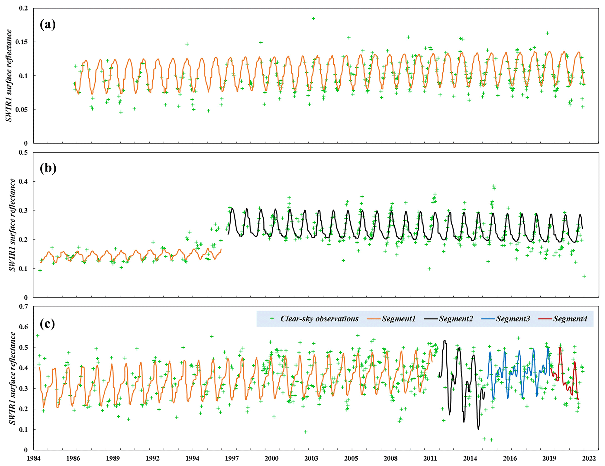
Figure 3 Three typical land-cover changes identified using the continuous change-detection (CCD) algorithm and continuous Landsat observations. The times series show (a) a stable land-cover condition, (b) a single abrupt change, and (c) multiple abrupt changes.

3.3 Updating changed areas using local adaptive classifications

Using the CCD algorithm and continuous Landsat imagery, we identified the temporally stable pixels and the time points of abrupt changes for the land-cover change pixels. Accurately determining the land-cover labels of the changed pixels (or understanding the “from–to” change process) is another key procedure for land-cover time-series monitoring. To achieve this goal, we derived spatiotemporally stable training samples (see Sect. 3.3.1), updated the changed pixels using multitemporal classifications, and finally minimized the cumulative error caused by independent classifications.

3.3.1 Deriving spatiotemporally stable training samples

Numerous studies have demonstrated that the accuracy of the training samples plays a critical role in accurate mapping (Foody and Arora, 2010; Zhang et al., 2020). Visual interpretation can ensure high-confidence samples, but it requires a lot of manual participation, so it is not suitable for collecting large-area training samples. An alternative option involves generating training samples by refining existing land-cover products through a series of improvement measures (X. Zhang et al., 2021b; Zhang et al., 2023). Inspired by the latter option, we combined the GLC_FCS30-2020 prior dataset and the change-detection mask (derived using the CCD algorithm described in Sect. 3.2) to obtain the spatiotemporally stable training samples. Specifically, temporally stable areas are known to have higher mapping accuracy (Yang and Huang, 2021; Zhang and Roy, 2017; Zhang et al., 2023); thus, we first used the aforementioned CCD mask to retain the areas that were temporally stable during 1985–2022, and then we overlapped them with the GLC_FCS30-2020 maps to determine their land-cover labels. Next, because Radoux et al. (2014) emphasized that land-cover transition areas are usually subject to more serious misclassification problems and that pixels with homogeneous land cover have a higher probability of achieving acceptable accuracy, we used a morphological erosion filter of 3 pixels × 3 pixels to refine these temporally stable areas into spatiotemporally homogeneous areas.

The spatiotemporally stable areas identified using the check for temporal stability during 1985–2022, spatial homogeneity analysis, and the GLC_FCS30-2020 product (which have an overall accuracy of 82.5 %) were retained to generate the training samples. It should be noted that these spatiotemporally stable areas are not guaranteed to be completely accurate; that is, a small number of the derived training samples may have been mislabeled. Fortunately, previous studies of large-area land-cover mapping demonstrated that the random forest classification model (adopted in this study; see Sect. 3.3.2) is highly robust to erroneous training samples (Gong et al., 2019b; Mellor et al., 2015; X. Zhang et al., 2021b). For example, Gong et al. (2019b) found that the overall accuracy remained relatively stable provided the proportion of erroneous training samples was within 20 %. This provides support for the use of the spatiotemporally stable areas to derive confident training samples and further ensures the quality of land-cover dynamics monitoring.

Numerous studies have highlighted the importance of the training sample balance and distribution, as they significantly influence the mapping performance (Foody, 2009; Jin et al., 2014; Millard and Richardson, 2015). First, there are two options for the training sample distribution: areal-proportional or equal allocation. The former was shown to achieve higher accuracy than the latter option in land-cover mapping, especially in complicated land-cover conditions (Jin et al., 2014). However, when using the areal-proportional sampling strategy, the rare land-cover types usually had small sample sizes and were sacrificed because the aim of land-cover mapping was to achieve a global optimum rather than a local optimum. Thus, the study of Zhu et al. (2016) suggested maximum and minimum sample sizes for abundant and rare land-cover types of 8000 and 600, respectively, to avoid the use of extremely large or small sample sizes. Thus, the GLC_FCS30-2020 product was then split into 961 5° × 5° geographical tiles, and we used the areal-proportional sampling strategy and two sample balancing thresholds to allocate the training samples from the spatiotemporally stable areas in each 5° × 5° geographical tile. Lastly, the impervious surface and wetland samples were excluded because both were independently developed as thematic datasets in Sects. 2.3 and 2.4.

3.3.2 Updating changed areas using local adaptive classifications

Before building the local adaptive classification models, we had to extract useful spectral features from the Landsat time-series observations. In this study, we used multitemporal phenological, texture, and topographical features. Specifically, the multitemporal phenological features were extracted by using the percentile-compositing method, which has fewer constraints than other compositing algorithms (such as the season-based compositing method) but achieves similar mapping accuracy (Azzari and Lobell, 2017). The spectral bands for the Landsat time series (five optical bands after excluding the atmospherically sensitive blue band) and the corresponding spectral indexes (NDVI, NDWI, and NBR in Eq. 2) were composited into five percentiles (10th, 25th, 50th, 75th, and 90th). Next, our previous study explained that the texture features made a positive contribution to land-cover mapping (X. Zhang et al., 2021b), so the gray-level co-occurrence matrix method was used for the 50th-percentile-composited NIR band to extract the homogeneity, entropy, dissimilarity, variance, contrast, and correlation. Lastly, since the land-cover distribution is usually related to the topographical environment (for example, croplands and water bodies are mainly distributed in flat areas), three topographical variables (elevation, slope, and aspect) calculated from a global 30 m DEM dataset named ASTER_GDEM (Tachikawa et al., 2011) were also imported. In addition, due to the limited storage capacity and satellite–ground data-transmission capacity of early satellites, the density of Landsat imagery is sparse before 2000 (only a single satellite, Landsat 5, acquired data) (Roy et al., 2014b). Thus, we chose a coarse temporal cycle of 5 years to ensure the mapping accuracy before 2000; that is, the satellite observations from 2 years before and after were used for the nominal center year. For example, we updated the land-cover maps in 1995 using all available imagery from 1993 to 1997. In total, there were 49 multisource features, including 40 phenological spectra features, 6 texture features, and 3 topographical variables.

There are two options for global land-cover mapping and updating: global modeling and local adaptive modeling, and our previous studies have found that local adaptive modeling yields superior results compared to global modeling. This is primarily due to the former's capability to take regional characteristics into account more effectively, leading to increased sensitivity in training samples and higher accuracy in land-cover classification (X. Zhang et al., 2021b, 2023, 2022). Thus, we first inherited the regional gridding style used in the GLC_FCS30 (X. Zhang et al., 2021b); namely, the global land was divided into 961 5° × 5° geographical tiles. Afterward, the local classification models were independently built to update the land cover in each tile using the corresponding training samples in the neighboring eight surrounding tiles in a 3×3 window. The adjacent training samples were imported to increase the continuity of the adjacent land-cover maps.

Lastly, in relation to the selection of the most suitable classification algorithm, the random forest (RF) classifier has significant advantages, including its capacity to accommodate high-dimensional training features and its better ability to deal with the overfitting problem and higher classification accuracy than other widely used classifiers (Belgiu and Drãguþ, 2016; Gislason et al., 2006). The RF algorithm was also integrated into the internal function library of the GEE cloud platform as ee.Classifier.smileRandomForest(). Thus, the RF algorithm was used to combine the training samples and multisourced features to update the changed pixels. The RF algorithm allows for the adjustment of two key parameters (the number of decision trees (Ntree) and the number of predicted variables (Mtry), and previous studies have quantitatively analyzed the relationships between classification accuracy and the values of these two parameters. Both theoretical and experimental results indicated that the selection of Mtry and Ntree had little influence on the classification accuracy (Belgiu and Drãguþ, 2016; Du et al., 2015). Thus, based on previous studies (Belgiu and Drãguþ, 2016; Zhang et al., 2019), the default recommended values of 500 for Ntree and the square of the total number of input features for Mtry were used.

3.3.3 Temporal-consistency optimization

To ensure the rationality and consistency of land-cover changes for long time series, the CCD algorithm was applied to capture the time points of land-cover changes, and then the changed pixels were updated using the local adaptive classifications. In this study, despite our best efforts, it was difficult to completely eliminate classification errors, particularly when dealing with changes over time. To address this issue and enhance accuracy in areas with temporal variations, we employed the temporal consistency optimization method described in Eq. (3). This approach incorporates both temporal and spatial neighboring information to assess homogeneity, thereby reducing potential misclassifications of changed areas in the time series.

$$\begin{array}{}\text{(3)}& \begin{array}{rl}{P}_{x,y,t}& ={\displaystyle \frac{\mathrm{1}}{N}}\left[{\sum }_{x^{\prime }=x-\mathrm{1}}^{x^{\prime }=x+\mathrm{1}}{\sum }_{y^{\prime }=y-\mathrm{1}}^{y^{\prime }=y+\mathrm{1}}{\sum }_{t^{\prime }=t-\mathrm{1}}^{t^{\prime }=t+\mathrm{1}}\right.\\ & \left.\cdot I\left(L_{x^{\prime },y^{\prime },t^{\prime }}=L_{x,y,t}\right)\right]\end{array}\end{array}$$

Here, $P_{x,y,t}$ is the homogeneity probability of the pixel at spatial location (xy) and time point t; usually, the higher the value of $P_{x,y,t}$, the weaker the classification error effect. $L_{x,y,t}$ and $L_{x^{\prime },y^{\prime },t^{\prime }}$ are, respectively, the land-cover labels of the central pixel and the corresponding spatiotemporally neighboring pixels in a local window of $\mathrm{3}\times \mathrm{3}\times \mathrm{3}$, and I() denotes the indicator function for the equation of the status between two pixels. Namely, if $L_{x^{\prime },y^{\prime },t^{\prime }}$ is equal to $L_{x,y,t}$, then the value of the indicator function is 1; otherwise, it is equal to 0 (Kenny, 2003). In this study, the homogeneity probability was calculated for each changed pixel, and a threshold of 0.5 (as suggested by and used in the studies of Li et al., 2015 and Zhang et al., 2022) was used to judge the rationality of land-cover changes; namely, when $P_{x,y,t}$ was less than the threshold, $L_{x,y,t}$ was modified according to the spatiotemporal pixels.

3.4 Accuracy assessment

The validation process for the GLC_FCS30D dataset followed the recommended guidelines proposed by Pontus Olofsson (2014). These guidelines encompass two key components: area estimation (non-site-specific accuracy) and accuracy assessment (site-specific accuracy). The site-specific accuracy assessment mainly focuses on estimating the confusion matrix and calculating some accuracy metrics, including overall accuracy (O.A.), producer's accuracy (P.A.), and user's accuracy (U.A.); and a poststratified estimator is used to calculate the corresponding standard errors (Pontus Olofsson, 2014).

$$\begin{array}{}\text{(4)}& \begin{array}{rl}& {\text{P.A.}}_k={\displaystyle \frac{p_{kk}}{\sum p_{k.}}}\\ & {\text{U.A.}}_k={\displaystyle \frac{p_{kk}}{\sum p_{.k}}}\\ & \text{O.A.}={\sum }_{k=\mathrm{1}}^m{p}_{kk}\end{array}\end{array}$$

Here, p_kk is the proportion of the area mapped as class k that had a reference class of k; $\sum p_{k.}$ and $\sum p_{.k}$ are the proportion of the area mapped as class k and the proportion of the reference area mapped as class k, respectively; and m denotes the number of land-cover types. Afterwards, because there is currently no global long-time-series validation dataset, we used 84 526 global validation points to assess the accuracy metrics of the GLC_FCS30D dataset in 2020 and used two third-party datasets to analyze the variation across the accuracy time series. GLC_FCS30D adopts a fine classification system containing 35 subcategories, for which we applied an analysis protocol to the basic classification system and the LCCS level-1 validation system, whose details are explained in the Table 1 and contained 10 major land-cover types and 17 fine land-cover types. Lastly, to quantify the performance of land-cover changed pixels, we followed the proposal of Stehman et al. (2021) for assessing the LCMAP annual land-cover products for 1985–2017; that is, the validation pixels were grouped into “changed” and “unchanged” categories and the corresponding confusion matrix was calculated. Meanwhile, to minimize the imbalance in sample size between the “change” and “no-change” samples, the F1 metric score was calculated as

$$\begin{array}{}\text{(5)}& \text{F1}={\displaystyle \frac{\text{P.A.}\times \text{U.A.}}{\text{P.A.}+\text{U.A.}}}\times \mathrm{2}\times \mathrm{100}\mathit{\%}.\end{array}$$

4 Results and discussion

4.1 Overview of the GLC_FCS30D maps and their changes

Figure 4 provides an overview of the GLC_FCS30D dataset for 2022 (an overview of GLC_FCS30D for 1985 is given in Fig. S3); overall, it aligns with the real-world land-cover patterns on a global scale. Forest, cropland, barren land, and grassland are the dominant land-cover types, and each of them is distributed in the corresponding ecology subregions. For example, needle-leaved forest is mainly concentrated in the high-latitude cold regions, while broad-leaved forests are mainly distributed in tropical regions; permanent ice and snow are mainly located in Greenland and high-altitude mountains. GLC_FCS30D has significant advantages over other global land-cover datasets in terms of land-cover type diversity: it contains 35 discrete land-cover types, among which forests and wetlands are subdivided into 10 and 7 land-cover subcategories, respectively.

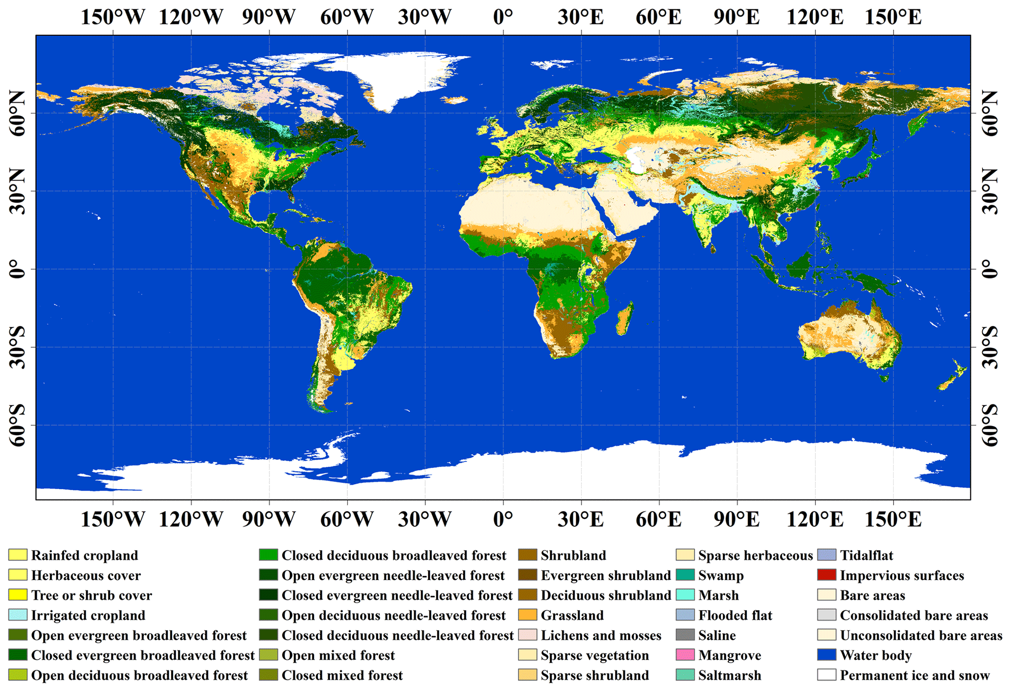
Figure 4 Overview of GLC_FCS30D for 2022; the color-coded legend is derived from the European Space Agency (ESA) Climate Change Initiative land-cover dataset (Defourny et al., 2018).

Figure 5a illustrates the spatial distribution of land-cover change intensity (measuring the proportions of changed pixels in the 0.05° grid) in GLC_FCS30D from 1985 to 2022 after upscaling to a resolution of 0.05°. Obviously, global land cover has experienced significant changes over the past 37 years, mainly in three areas: (1) areas on the periphery of tropical rainforests in South America and Southeast Asia, with deforestation the dominant cause; (2) areas where wetlands and water bodies intermingle (i.e., water bodies and wetlands transform into one another due to different annual water levels; note that the water body land-cover type in GLC_FCS30D represents permanent water during the year of interest, although the same area may be a wetland in other years), such as those in North America and northern Asia; and (3) semi-arid areas in Australia, Central Asia, and western Africa, where land cover (such as sparse vegetation or bare land) is directly affected by precipitation and temperature (for example, if there is sufficient precipitation in the year, the sparsely vegetated land and some of the bare land would be covered by grass in semi-arid areas; similarly, the work of Winkler et al., 2021 revealed that these semi-arid areas experienced serious and frequent land-cover changes). Figure 5b quantifies the changed area for 10 major land-cover types from 1985 to 2022. Forest and cropland variations dominated the global land-cover change. The net loss of forests over the past 37 years reached approximately 2.5 million km², and the decline has been steady over time. Conversely, cropland showed a stable increase, and the net gain in cropland area is approximately 1.3 million km². Shrubland, wetland, and impervious surface increased in area by 0.45 million, 0.40 million, and 0.37 million km², respectively. The increased shrubland resulted from the recovery of deforested land, and the wetland gains are due to increases in seasonal water bodies. The work of Pekel et al. (2016) emphasized that global seasonal water bodies (labeled “inland wetlands” in GLC_FCS30D) showed an overall increase.

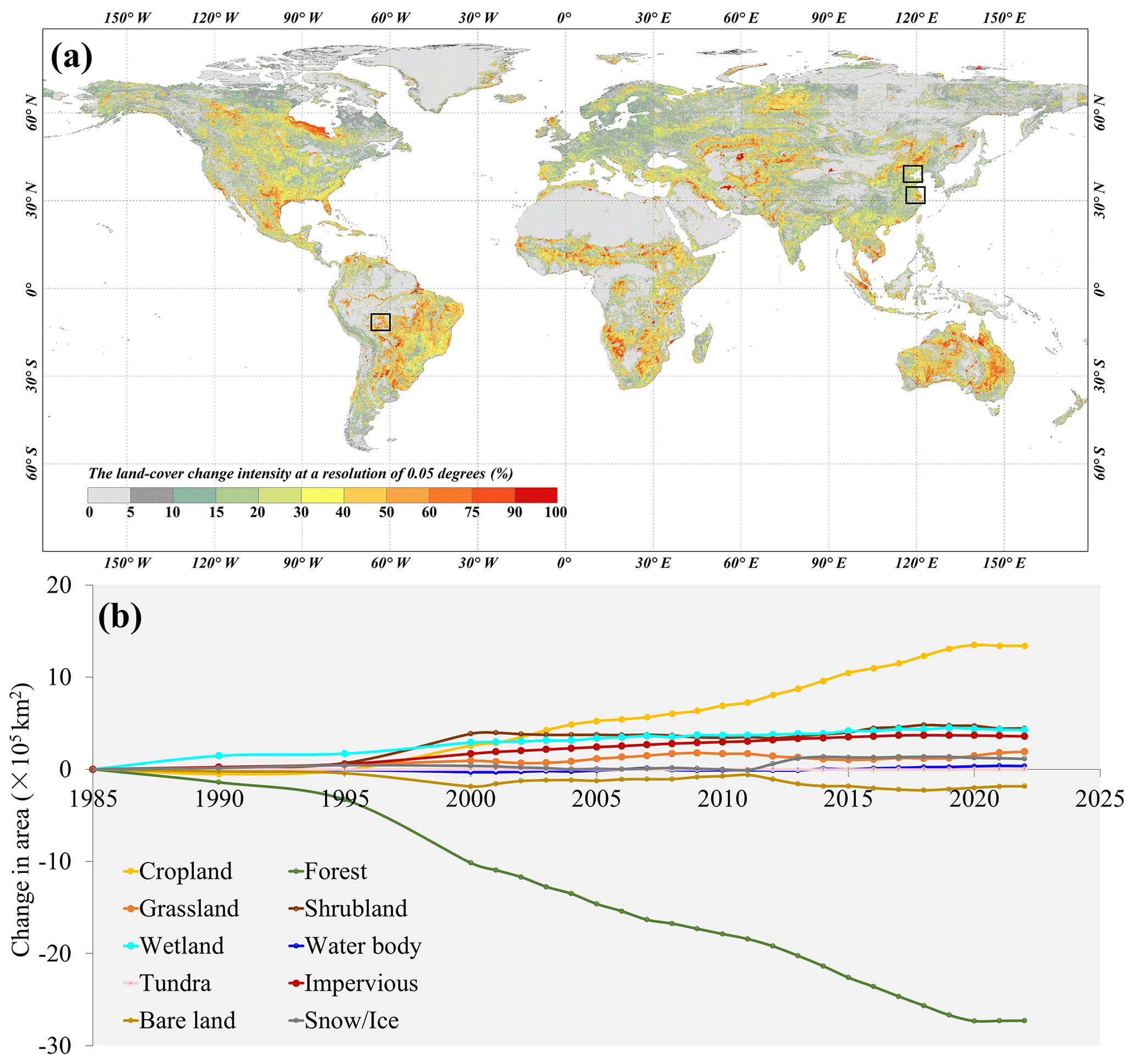
Figure 5 (a) The spatial distribution of global land-cover-change intensity from 1985 to 2022 after aggregation to a resolution of 0.05°. (b) The net changed area of 10 major land-cover types in GLC_FCS30D from 1985 to 2022.

Figure 6 further analyzes the net area variations of 10 major land-cover types on six continents. The six continents exhibit various land-cover change characteristics; for example, steady forest loss and cropland gain dominate land-cover change in South America, while the net area variations of most land-cover types fluctuate in Australia. North America has experienced obvious deforestation, and the area of forest loss reaches approximately 4.5×10⁵ km². In contrast, the shrubland, grassland, and impervious surface land-cover types show increasing trends overall, with increases of 1.4×10⁵ km², 0.8×10⁵ km², and 0.72×10⁵ km², respectively. Similarly, Xian et al. (2022) reported that forest losses and shrubland, grassland, and impervious surface gains were the dominant characteristics of the CONUS from 1985 to 2017. In Europe, the forest area continuously decreased, and the cropland area first decreased and then increased because of the collapse of the Soviet Union in 1990s. Abandoned croplands were transformed into pasture (which also belongs to the cropland land-cover type in GLC_FCS30D). Among the six continents, the increase in impervious surface is the most significant in Asia, with a net increase of 1.9×10⁵ km²; wetland also shows a large increase of 1.1×10⁵ km². The increased wetland coverage comes from the increase in seasonal water bodies. South America and Africa have experienced similar land-cover change characteristics: they show the most intense deforestation rates and the most significant increases in cropland. According to our statistics, the forest loss on these two continents amounts to 16.9×10⁵ km², and the corresponding increase in cropland is approximately 11.1×10⁵ km². Lastly, Oceania is more sensitive to climate change, especially in terms of precipitation, so fluctuations in shrubland, grassland, and bare land are evident there because the conversion relationship between the three land-cover types is related to annual precipitation.

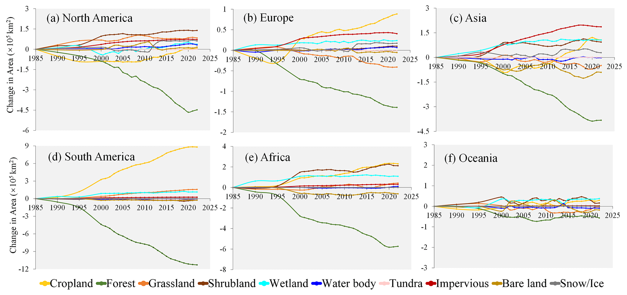
Figure 6 The net area variations of 10 major land-cover types on six continents from 1985 to 2022.

Figure 7 displays the land-cover transformation relationships from 1985 to 2022 in the GLC_FCS30D dataset using Sankey diagrams. Global cropland and forest show obvious area changes, with area proportions changing from 12.08 % and 38.26 %, respectively, in 1985 to 12.86 % and 36.48 %, respectively, in 2022. Shrubland changed from 8.70 % in 1985 to 9.03 % in 2022. We mainly focus on forest, cropland, shrubland, and impervious surface changes, which dominate the land-cover changes in Fig. 5. There are three main causes of forest loss over the past 37 years: (1) 37.58 % of the deforested land was converted to cropland (this transformation was more significant in tropical rainforest areas; Fig. 8a); (2) 26.92 % of the lost forest was regrown as shrubland, which is more common in mountainous areas affected by wildfires; and (3) 13.49 % of the deforested land was converted to grassland. Cropland is converted to forest, grassland, and impervious surfaces. A total of 26.29 % of the lost cropland is converted to grassland due to abandonment, 25.88 % of the lost cropland is covered by forests, and 21.01 % of the lost cropland resulted from urbanization. Lastly, regarding impervious surfaces, our primary focus was on identifying the sources contributing to their expansion. Our findings indicate that approximately 36.24 % of the impervious surface increase can be attributed to the conversion of cropland, while 13.49 % of the increase is a result of deforestation.

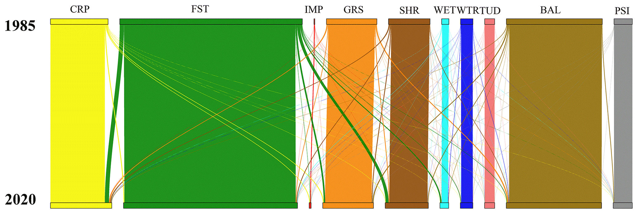
Figure 7 Sankey diagrams of the global land-cover changes during 1985–2022 in the GLC_FCS30D dataset.

To visually understand the land-cover change process captured by the GLC_FCS30D dataset over the past 37 years, Fig. 8 displays three typical enlargements (the spatial locations of the enlarged areas are illustrated as two black rectangles in Fig. 5a) of the Amazon rainforest (which experienced significant deforestation) and China's Yangtze River Delta (which underwent rapid urbanization) and Yellow River delta (which showed evident land-cover changes over coastal regions). These three typical areas experienced drastic land-cover changes, and GLC_FCS30D accurately captures those spatiotemporal changes. Specifically, the deforestation in South America is widely recognized, and GLC_FCS30D clearly reflects this trend. Namely, the early deforestation showed a grid distribution, and then each grid gradually extended outward and finally connected into patches. GLC_FCS30D also shows that deforestation has not stopped in the region in terms of the rate of forest loss, and these findings are in line with the results of earlier research (Harris et al., 2021; Potapov et al., 2022). In the Yangtze River Delta, GLC_FCS30D depicts that the dominant land-cover change over the enlargement is urbanization, and a large quantity of irrigated cropland has been converted to impervious surfaces. Meanwhile, urban expansion was significantly faster before 2010 than after 2010 according to GLC_FCS30D. Lastly, the Yellow River delta, a typical coastal region, was selected to assess the ability of GLC_FCS30D to capture these coastal land-cover changes. Obviously, the land-cover changes in GLC_FCS30D can be summarized as three aspects: (1) a large number of flooded flats and tidal flats were reclaimed as aquaculture ponds, especially after 2000; (2) the mouth of the Yellow River changed from a southerly orientation to a northerly one (black rectangle), i.e., there were large land-cover changes between tidal/flooded flats, water bodies, and salt marshes; and (3) a lot of impervious surfaces encroached on the coastal water bodies and flats. In short, by combining real remote-sensing observation time series data, GLC_FCS30D effectively captures the spatiotemporal changes of the land surface.

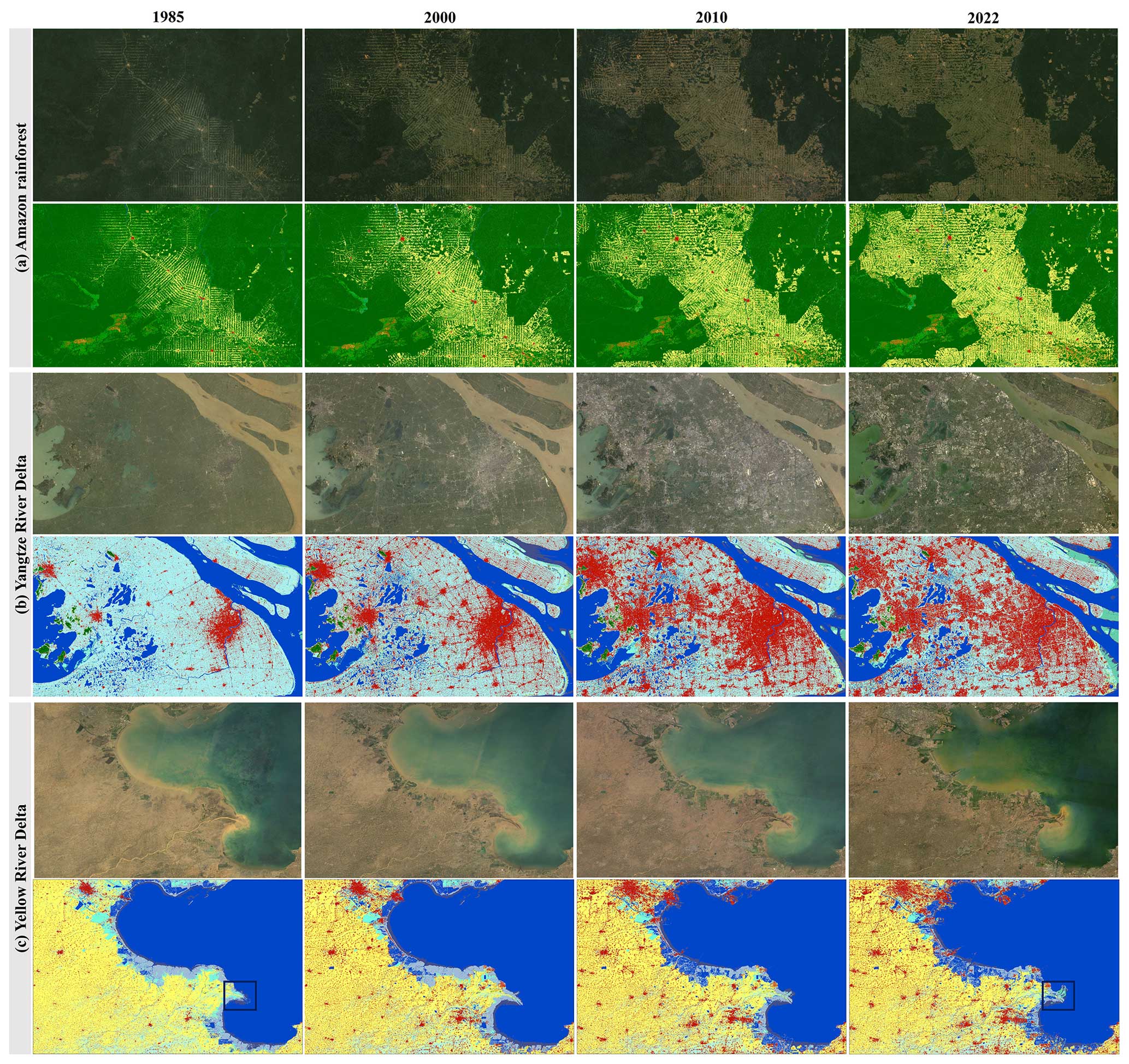
Figure 8 Three typical enlargements showing the land-cover changes according to GLC_FCS30D from 1985 to 2022 in (a) the Amazon rainforest, (b) the Yangtze River Delta in China, and (c) the Yellow River delta in China. The color coding is the same as that used for the global map in Fig. 4. In each case, the natural-color imagery from 1985 to 2022 are composites taken from Landsat imagery.

4.2 Accuracy assessment of GLC_FCS30D for 2020

Table 2 provides the error matrix and accuracy metrics for the GLC_FCS30D dataset in the basic classification system containing 10 major land-cover types. The novel GLC_FCS30D dataset attained an O.A. of 80.88 % (±0.27 %). Cropland, forest, impervious surface, water body, and permanent snow and ice perform better in terms of the P.A. and U.A. than the remaining land-cover types, with the corresponding accuracies exceeding 85 %. The impervious surface and wetland datasets are independently generated and then overlaid on GLC_FCS30D, helping these complicated land-cover types to achieve high accuracy metrics. Conversely, grassland, shrubland, and tundra have lower accuracies; for example, grassland had the lowest P.A. of 54.41 % and shrubland had the lowest U.A. of 57.63 %. The two reasons that they performed poorly were as follows: (1) these land-cover types usually reflected heterogeneous and varied spectral and spatial characteristics, e.g., the grassland showed similar spectra to cropland and sparse shrubland in the growing season but mimicked bare-land features in harvest season, and (2) all of them were distributed in climate-transition areas with complicated climate variations and landscapes.

Table 2 Error matrix of the GLC_FCS30D dataset for 2020 based on the basic classification system. The reported producer's accuracy (P.A.) and user's accuracy (U.A.) come with corresponding standard errors (SE) shown in parentheses.

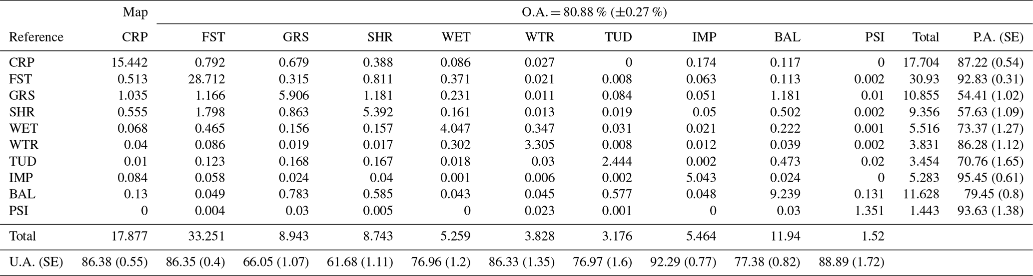
Note: the abbreviations correspond to the 10 categories of the basic classification system in Table 1.

Table 3 provides the error matrix of GLC_FCS30D for 2020 in the LCCS level-1 validation system with 17 land-cover types. The GLC_FCS30D-2020 dataset achieves an O.A. of 73.04 % (±0.30 %), which is lower than that achieved with the basic classification system because these similar land-cover subcategories suffer more easily from misclassification. For example, forest has a P.A. of 92.83 % (±0.31 %), but the P.A. rapidly decreases to the range of 58.29 % (±1.53 %) to 82.39 % (±0.98 %) when forest is split into five fine subcategories. Cropland, forest, and bare land, which are further divided into multiple subcategories, show obvious decreases in accuracy for their subcategories in terms of P.A. and U.A. Taking cropland and forest as examples, approximately 31.7 % of the irrigated cropland (ICP) is misclassified as rainfed cropland (RCP), and so the U.A. of ICP is only 59.92 %. More than 53.8 % of the mixed-leaf forests (MFT) are wrongly labeled as the other four forest subcategories, and so the `mixed-leaf forests have the lowest U.A. of 39.34 % (±1.38 %). Meanwhile, sparse vegetation has the second lowest U.A. of 50.63 % (±1.47 %) because of the confusion between sparse vegetation, grassland, and bare land. In the basic classification system (Table 1), sparse vegetation is grouped with bare land. A previous study in the European Union proposed grouping it with grassland (Gao et al., 2020). Wetland is further divided into coastal wetland (CWL) and inland wetland (IWL) in Table 3, and CWL has a higher U.A. than that of wetland in Table 2, which is primarily attributable to the significantly more accurate classification of wetland in the CWL subcategory (Zhang et al., 2023).

Table 3 Error matrix of the GLC_FCS30D dataset for 2020 based on the LCCS level-1 validation system. The reported producer's accuracy (P.A.) and user's accuracy (U.A.) come with corresponding standard errors (SE) shown in parentheses.

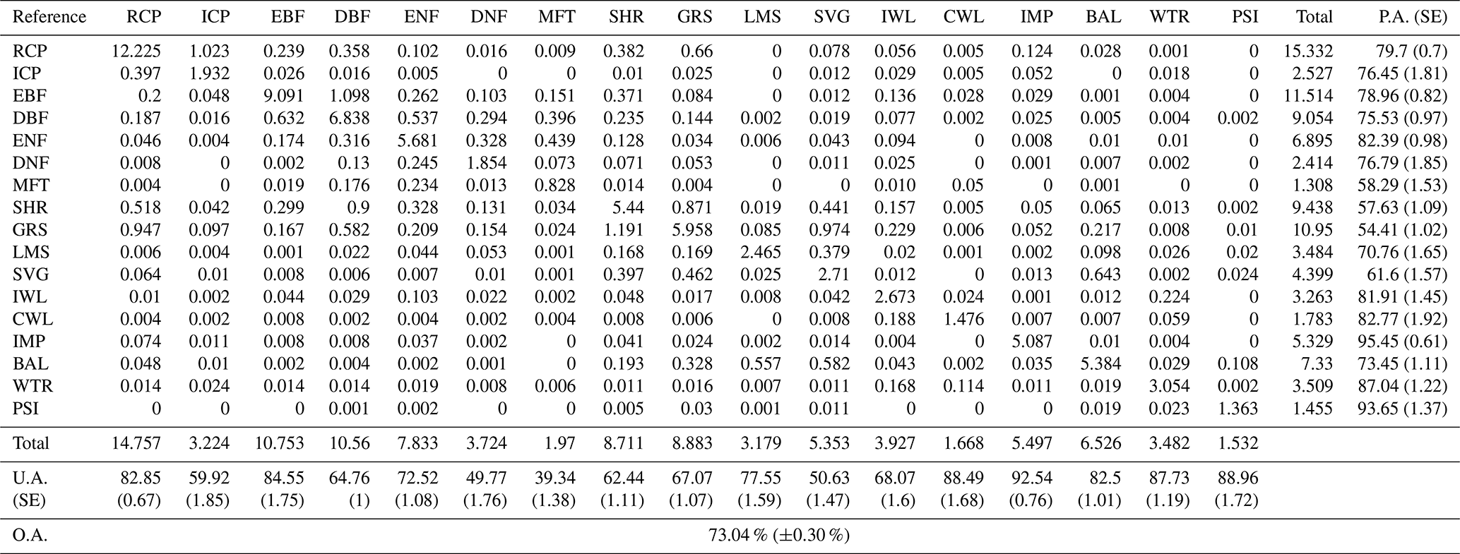
Note: the abbreviations correspond to the 17 categories of the LCCS validation system in Table 1.

4.3 Accuracy assessment based on two third-party regional validation datasets

4.3.1 Time series of accuracy metrics of GLC_FCS30D from the LCMAP_Val dataset

Figure 9 displays a time series of the overall accuracy of the GLC_FCS30D dataset using the LCMAP_Val annual validation dataset from 1985 to 2018 over the CONUS. GLC_FCS30D achieves a mean O.A. of 79.50 % (±0.50 %) and the O.A. varies from a high value of 80.04 % (±0.49 %) in 2015 to a low value of 78.91 % (±0.51 %) in 2000. The overall accuracy of GLC_FCS30D is slightly lower at the early stage, which might be related to the density of Landsat observations. The early Landsat missions had weaker satellite-to-ground transmission and onboard recording capabilities (Roy et al., 2014a), so the phenological variability and land-cover changes were more difficult to capture at the early stage.

Figure 9 Time series of the overall accuracy of the GLC_FCS30D dataset using the LCMAP_Val annual reference dataset across the contiguous United States (CONUS) from 1985 to 2018. The error bars on the graph show the uncertainty of the data points.

Figure 10 shows time series of the P.A. and U.A. for the GLC_FCS30D dataset in the CONUS. Visually, the P.A. and U.A. values of the 10 major land-cover types range from 45 % to 100 % and from 35 % to 100 %, respectively, and the time-series variations are stable. Among them, the water body land-cover type has the highest accuracy metrics, achieving mean P.A. and U.A. values of 95.31 % (±1.14 %) and 98.53 % (±0.66 %), respectively, which benefit from the unique spectral characteristics of this land-cover type. Cropland follows, with mean P.A. and U.A. values of 93.37 % (±0.74 %) and 87.70 % (±0.94 %), respectively. Forest ranks third, with a high P.A. of 97.75 % (±0.35 %) but a relatively low U.A. of 82.42 % (±0.82 %); the unbalanced metrics occur because GLC_FCS30D and LCMAP_Val have different definitions for forest. GLC_FCS30D defines a forest as having a tree cover greater than 15 %, while the threshold setting of LCMAP_Val is 10 %, so many of the shrublands in GLC_FCS30D are labeled as forests in LCMAP_Val. Wetland has a U.A. value of 90.47 % (±2.05 %) but a P.A. value of 57.07 % (±2.75 %), which is also caused by a discrepancy in the definition of wetland. GLC_FCS30D identifies seasonal water bodies as wetlands while LCMAP_Val classifies them as water bodies. Impervious surface has a P.A. lower than 60 %, mainly because the GLC_FCS30D and LCMAP_Val datasets have different definitions of impervious surface. LCMAP_Val defines buildings and the surrounding green areas as developed, while GLC_FCS30D only includes the artificial buildings (houses, roads, squares, and so on). Bare land and shrubland have the lowest U.A. values of 35.58 % (±4.39 %) and 47.29 % (±1.56 %), respectively, mainly because both of them are easily confused with grassland due to their complicated spectral characteristics and because they coexist in climate-sensitive semi-arid regions (e.g., the Midwestern United States). Xian et al. (2022) emphasized that long-term monitoring of shrubs and grasslands presents significant challenges in the CONUS. Permanent snow and ice, which is sparsely distributed in high-elevation mountainous areas of the United States, has unique and specific spectral characteristics, so it achieves a P.A. of 100 % in GLC_FCS30D. The large fluctuations in U.A. for ice and snow are attributed to (1) the small sample size for ice and snow in the LCMAP_Val dataset and (2) a few misclassified grass/bare land pixels that are correctly identified as snow and ice during 2005–2014.

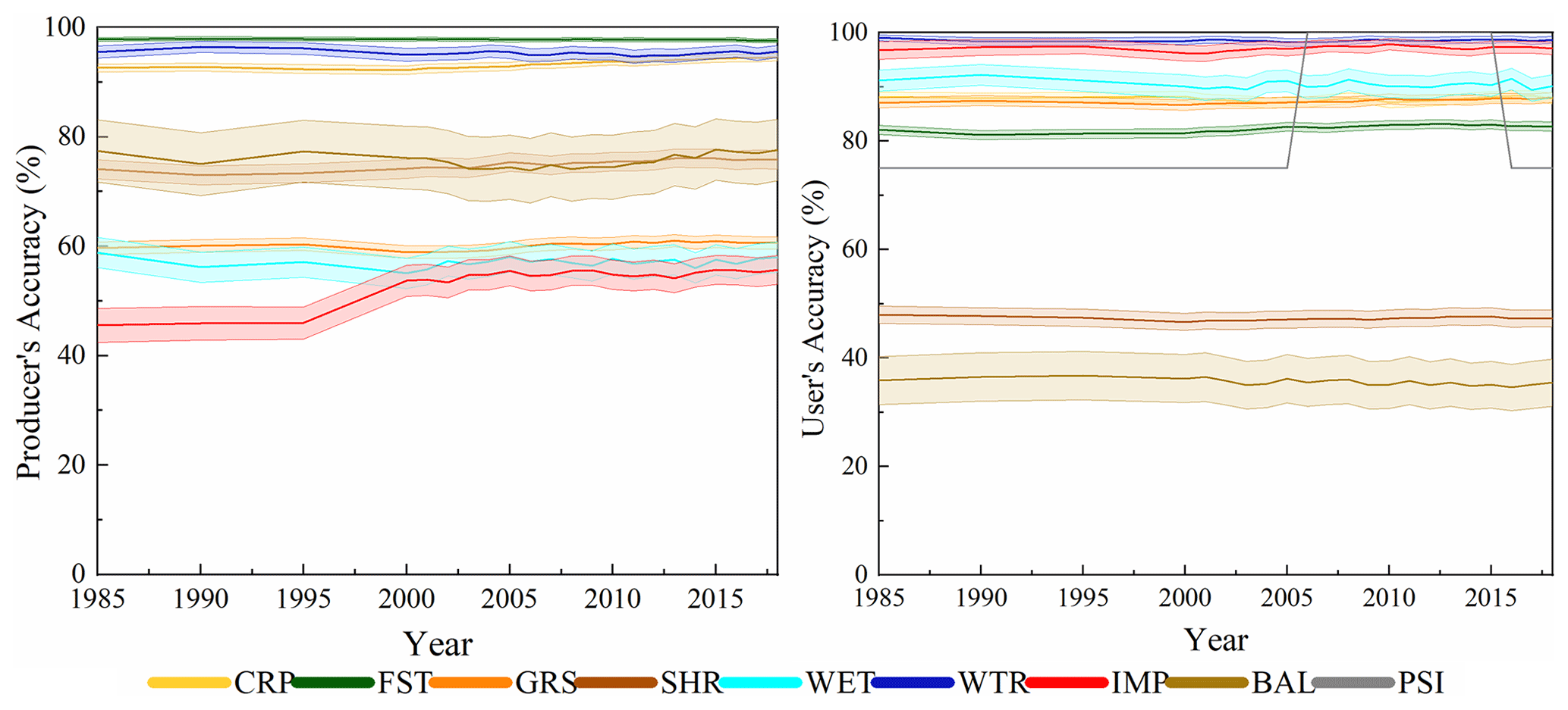
Figure 10 Time series of the producer's accuracy and user's accuracy of GLC_FCS30D based on the LCMAP_Val dataset from 1985 to 2018 in the contiguous United States (CONUS). The error bands represent ±1 standard error.

Figure 11 shows the area-bias percentages of eight land-cover types estimated by GLC_FCS30D and LCMAP_Val across the CONUS. Intuitively, GLC_FCS30D and LCMAP_Val share similar total areas for estimations of cropland, bare land, and water bodies but evident area deviations for estimations of forest, shrubland, and grassland. The deviations in shrubland and grassland occur mainly because these land-cover types coexist in the semi-arid regions of the central United States and share similar spectral characteristics and temporal variability; thus, some grasslands in LCMAP_Val are considered shrublands in GLC_FCS30D. Xian et al. (2022) also failed to distinguish grassland from shrubland and combined them into a group when generating LCMAP annual maps. LCMAP_Val has a broader definition of impervious surface, which results in negative bias, so the impervious surface area estimated in LCMAP_Val is larger than the assessment in the GLC_FCS30D dataset.

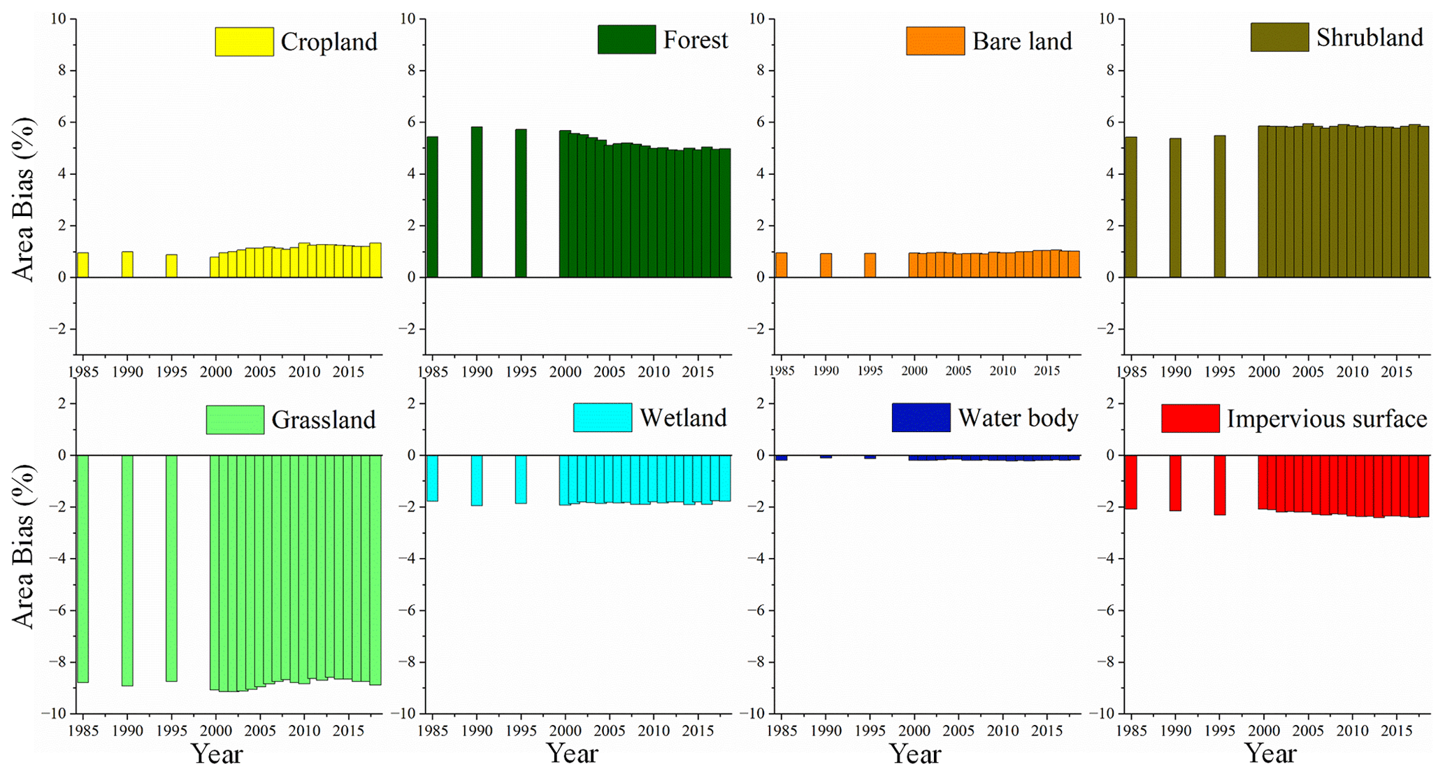
Figure 11 The area-bias percentages of eight land-cover types in the GLC_FCS30D and LCMAP_Val datasets from 1985 to 2017 in the contiguous United States (CONUS).

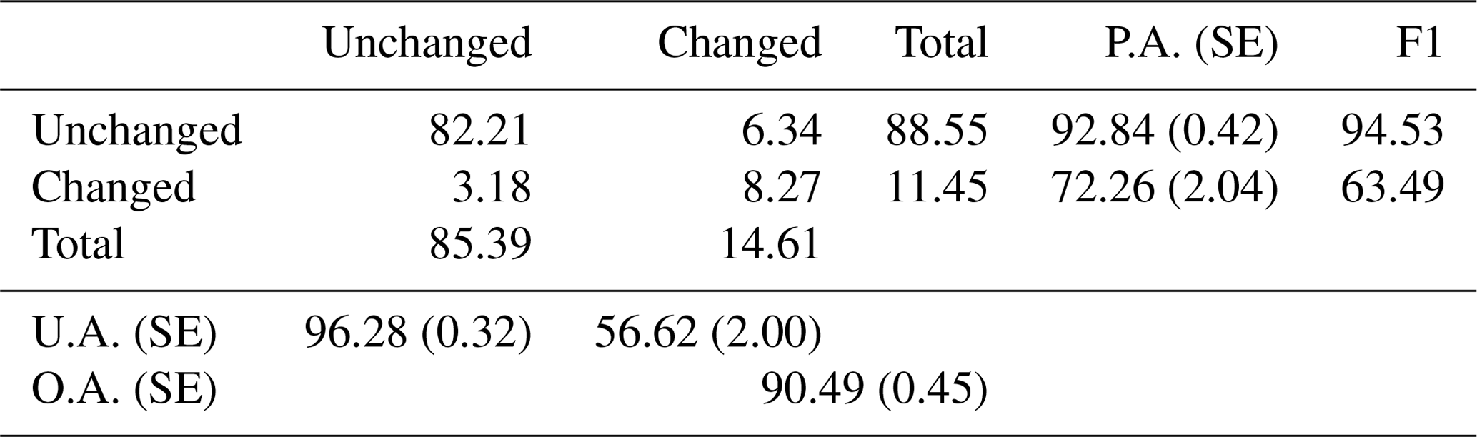
Table 4 analyzes the confusion matrix of changed and unchanged land-cover pixels in GLC_FCS30D using the LCMAP_Val dataset. It should be noted that the changed land-cover samples in LCMAP_Val were still sparse; that is, the size of the changed samples cannot support the analysis of specific land-cover changes. Similarly, Stehman et al. (2021) grouped the land-cover types into “no change” and “change” types for analyzing the land-cover changes. In this study, when using the “changed” and “unchanged” validation points in LCMAP_Val, the O.A. of GLC_FCS30D reached 90.49±0.45 %. In particular, the unchanged land-cover pixels played a dominant role and reached a high P.A. of 92.84 % and a high U.A. of 96.28 %. In contrast, the P.A. and U.A. of the changed land-cover pixels were 72.26±2.04 % and 56.62±2.00 %, and the F1 score was 63.49 %.

Table 4 The confusion matrix of changed and unchanged pixels in GLC_FCS30D when using the LCMAP_Val datasets.

4.3.2 Time series of accuracy metrics of GLC_FCS30D from the LUCAS dataset

Table 5 lists the time series of accuracy metrics of the GLC_FCS30D dataset across the European Union (EU) from 2006 to 2018 using the LUCAS dataset. The GLC_FCS30D dataset has a mean O.A. of 81.91 % (±0.09 %) and an O.A. range of 81.64 % (0.09 %) to 82.11 % (0.09 %) in the EU. The two dominant land-cover types (cropland and forest), which cover almost 70 % of the entire EU area (Gao et al., 2020), have higher P.A. and U.A. values than the other land-cover types. The P.A. and U.A. of cropland exceed 85 % and 93 %, respectively. Forest has unbalanced P.A. (approximately 95 %) and U.A. (approximately 76 %) values because the LUCAS dataset defines forest more broadly than the GLC_FCS30D dataset does. In particular, sparse vegetation associated with forest is grouped with forest in LUCAS but with bare land in GLC_FCS30D. Gao et al. (2020) explained the discrepancy in the definition of forest between LUCAS and GLC_FCS30. Shrubland, grassland, and bare land showed inferior performance in terms of both P.A. and U.A. because of their complicated spectral variability and spatial heterogeneity. Gao et al. (2020) also found that three global 30 m land-cover products (GlobeLand30, FROM_GLC, and GLC_FCS30) exhibited poor performance for these three land-cover types. Urban green space and discontinuous urban fabric, which are excluded from GLC_FCS30D, are grouped with impervious surface in LUCAS. Thus, impervious surface also has a low P.A. of approximately 59 %. Lastly, upon investigating the temporal variability of P.A. and U.A.  we find that permanent ice and snow and wetland show greater variability and that both are closely related to annual temperature and precipitation; i.e., their spatial distributions are affected by the natural environment.

Table 5 Time series of accuracy metrics of the GLC_FCS30D dataset using the LUCAS validation dataset across the European Union.

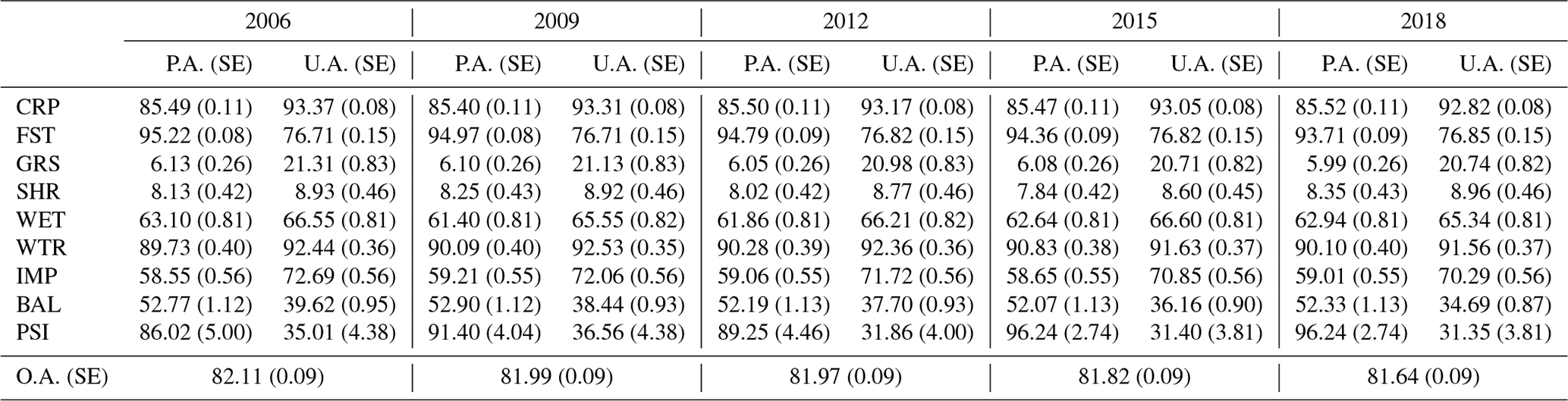
Table 6 shows the area proportions of 10 major land-cover types from both the GLC_FCS30D dataset (“Map”) and the LUCAS validation dataset (“Ref”). The area bias (“AB”) measures the area deviations between the two different datasets for the same land-cover type. Overall, GLC_FCS30D overestimates the total area assessments of forest, bare land, and ice and snow and underestimates the remaining land-cover types in comparison to the LUCAS estimations. In particular, according to its AB of +7.356 %, forest shows the most significant overestimation, while cropland shows the most underestimation (AB of −4.086 %). Cropland and forest cover together account for approximately 70 % of the total EU area (Gao et al., 2020)); as a result, the area bias (AB) values for these two land-cover types are more noticeable or pronounced compared to the AB values of the other land-cover types.

Table 6 The area proportions and area bias (AB) values of 10 major land-cover types from the GLC_FCS30D dataset (Map) and the LUCAS validation dataset (Ref).

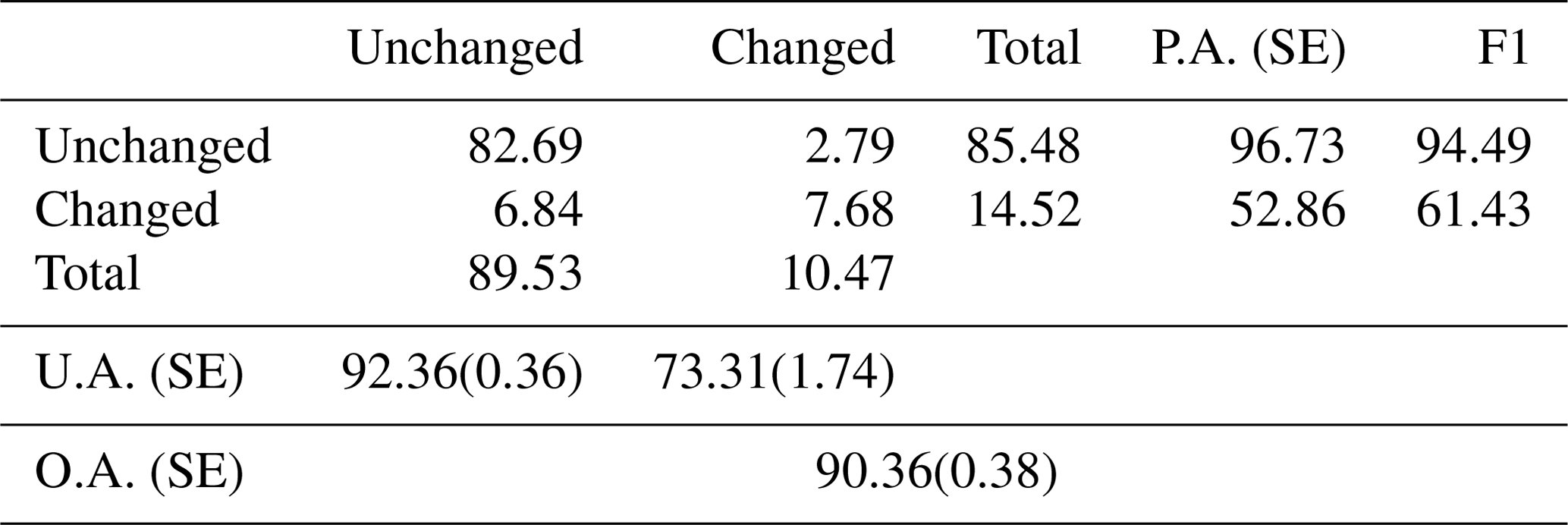
Table 7 presents the confusion matrix of changed and unchanged pixels obtained using the LUCAS validation datasets. The O.A. of GLC_FCS30D reached 90.36±0.38 %; the P.A. and U.A. of the changed pixels were 52.86±1.93 % and 73.31±1.74 %, respectively; and the corresponding F1 score was 61.43 %. In contrast, the unchanged land-cover pixels reached high P.A. and U.A. values, with both metrics exceeding 90 %. Thus, the changed land-cover pixels were more difficult to capture compared with these unchanged pixels. Similarly, Stehman et al. (2021) also found that the accuracy metrics of the changed pixels were far lower than those of the unchanged pixels: the producer's accuracy of the changed pixels and unchanged pixels was 16 % and 99 %, respectively.

Table 7 The confusion matrix of changed and unchanged pixels in GLC_FCS30D when using LUCAS time-series datasets across the Europe Union.

4.4 Comparisons with other global land-cover dynamics products

Figure 12 gives qualitative comparisons between our GLC_FCS30D and two widely used land-cover dynamics datasets (CCI_LC and MCD12Q1) for 2001–2020 in the Indo-China Peninsula, which experienced evident land-cover changes in terms of forest deforestation and urban expansion during that period. In terms of urban expansion, the three datasets revealed rapid urbanization in the megacity of Bangkok, while CCI_LC underestimated the impervious surface area in 2001 compared with the other two datasets. Meanwhile, GLC_FCS30D also captured more spatial detail (such as rural buildings and road networks) than CCI_LC and MCD12Q1 because of its high spatial resolution of 30 m.

In terms of the most significant deforestation, CCI_LC showed the worst performance because (1) it underestimated the forest cover in 2001 (rectangular region 1: R1), i.e., some forests were wrongly labeled croplands; (2) some deforested areas were not captured during the period 2001–2020 in rectangular region 2 (R2), so its deforested forest area was less than in GLC_FCS30D and MCD12Q1; and (3) there was an obvious problem with the misclassification of forest as wetland in 2001 (rectangular region 3: R3). MCD12Q1 also suffered from a forest omission error in R1; namely, the captured forest area in 2001 was lower than the actual forest area based on natural-color imagery. As for the evident deforestation in R2, we find that almost all forest pixels changed to the other land-cover types (savanna and grassland) in MCD12Q1, which obviously deviated from the actual situation; thus, MCD12Q1 overestimated the forest deforestation. Meanwhile, the MCD12Q1 time series showed various land-cover distributions in R3, which indicated that MCD12Q1 has lower mapping accuracy and temporal stability for these wetland areas. In comparison, GLC_FCS30D achieved the best performance in capturing the spatial distribution of forest in 2001, deforestation during 2001–2020, and wetland stability.

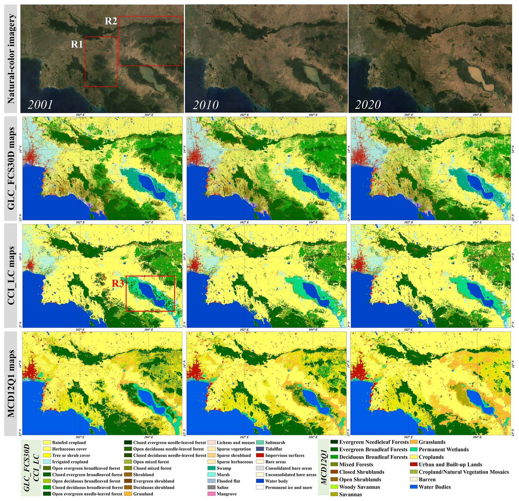
Figure 12 Comparisons of GLC_FCS30D with the CCI_LC and MCD12Q1 land-cover dynamics products for the Indo-China Peninsula during 2001–2020. The natural-color imagery were composited from the time-series Landsat imagery.

Figure 13 shows another comparison example for these three datasets, focusing instead on Paraguay, South America. The most evident land-cover changes were deforestation and increased cropland according to the time seriies of Landsat natural-color imagery. In terms of the spatial distribution, the consistency between GLC_FCS30D and CCI_LC was higher, while MCD12Q1 was obviously different from the other two datasets. A large number of deciduous broadleaved forests were labeled as savanna and woody savanna, and most croplands were identified as grasslands in MCD12Q1, mainly because of the difference in classification system. In terms of the changed-land-cover areas, the GLC_FCS30D showed the highest accuracy and captured richer spatial detail. For example, the deforestation intensity during 2010–2020 was significantly greater than that during 2001–2010, and GLC_FCS30D also revealed the regular deforestation caused by human factors. In contrast, CCI_LC and MCD12Q1 captured neither the deforestation during 2010–2020 nor the small and fragmented changes (caused by human activities).

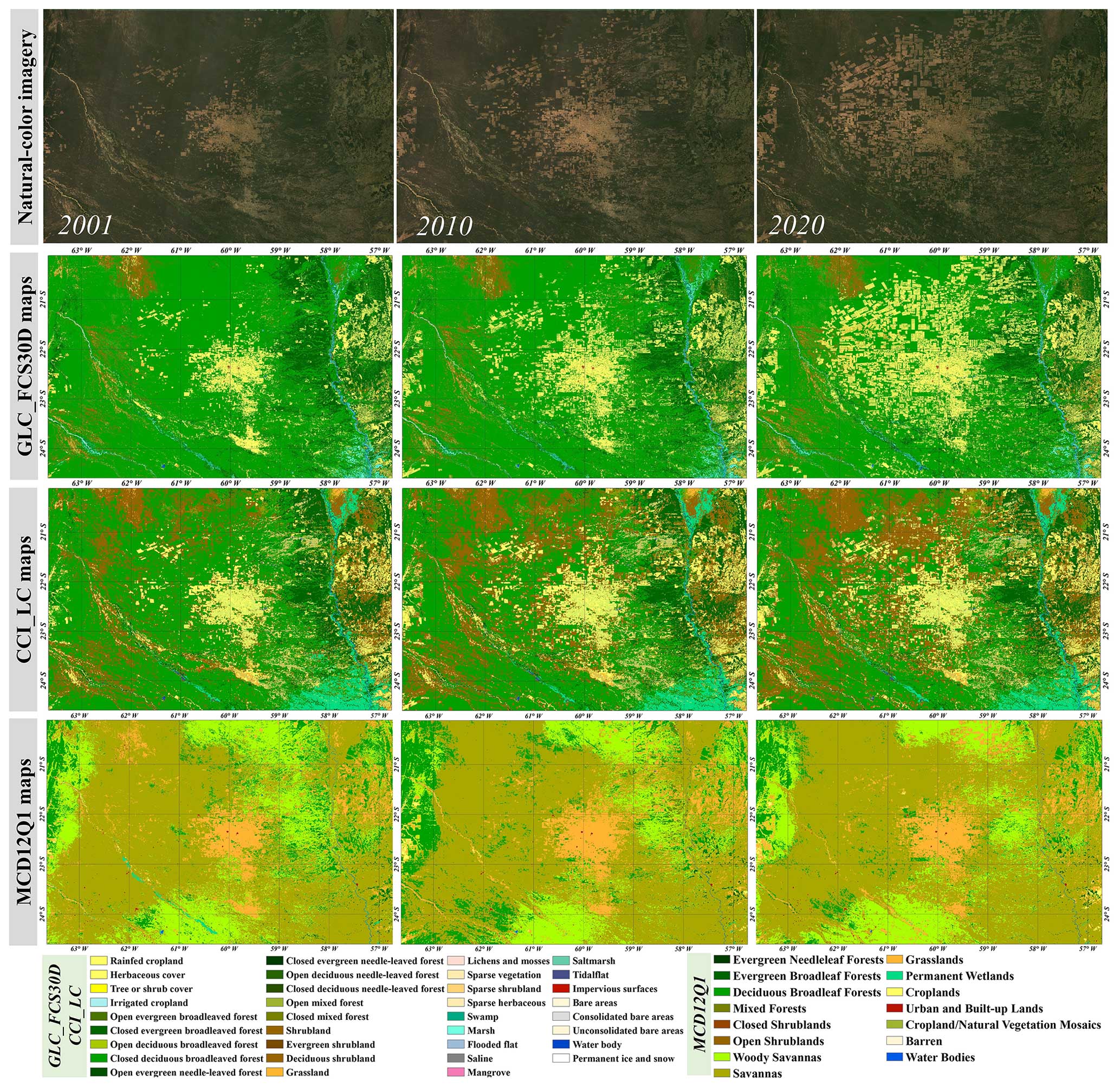
Figure 13 Comparisons of GLC_FCS30D with two land-cover-dynamics time-series datasets for Paraguay, South America, during 2001–2020. The natural-color imagery were composited from the time-series Landsat imagery.

4.5 Limitations of and perspectives on the GLC_FCS30D dataset

To achieve the goal of accurate and robust monitoring of global land-cover change, four steps are adopted: (1) the advantages of the CCD model and the full time series of Landsat observations are combined to capture the land-cover change time points for any changed pixels; (2) the temporally stable areas are used as prior knowledge to ensure the quality of training samples and local adaptive modeling is adopted to update the land-cover transitions of these changed pixels; (3) global thematic products for two complicated land-cover types (impervious surface and wetland) are independently developed to improve the reliability of GLC_FCS30D; and (4) the “spatiotemporal consistency checking” optimization in Sect. 3.3.3 is applied to further guarantee the stability and accuracy of GLC_FCS30D. The accuracy assessments performed using the developed global validation dataset and two third-party datasets demonstrate that GLC_FCS30D fulfills the accuracy requirements for a baseline year and for time-series variability at a global or national scale. Comparisons with other land-cover products also highlight the superiority of GLC_FCS30D in terms of classification system diversity and the monitoring accuracy of these changed areas. However, monitoring global land-cover change across a long time series is an extremely complex and difficult task (Hansen and Loveland, 2012; Song et al., 2018; Winkler et al., 2021; Xian et al., 2022). Although this study uses a series of measurements and methods to achieve global 30 m land-cover change monitoring for the past 37 years, there are still some uncertainties and limitations that need to be resolved in further work.

The CCD algorithm makes full use of dense satellite observations to capture land-cover changes robustly and accurately (Zhu and Woodcock, 2014b; Zhu et al., 2012). However, previous studies have demonstrated that their reliability is highly correlated to the density of valid satellite observations (Bullock et al., 2022; Ye et al., 2021; Zhu et al., 2019). Cloudy and snowy areas lead to greater uncertainty when capturing the time points of land-cover change (DeVries et al., 2015; Xian et al., 2022). Additionally, due to the limited storage capacity and satellite–ground data-transmission capacity of early satellites, the density of Landsat imagery is sparse before 2000 (only a single satellite, Landsat 5, acquired data) (Roy et al., 2014b). In this study, we combine the satellite observations from 2 years before and after the nominal center year from 1985 to 1995; for example, we update the land-cover maps in 1995 using all available imagery from 1993 to 1997. However, a previous study found that northeastern Asia did not have any valid Landsat observations before 2000 (Zhang et al., 2022), which means that some land-cover changes could not be captured in these areas before 2000 in GLC_FCS30D. To solve the problem of missing and sparse observations, a useful solution is to fuse multisourced remote-sensing imagery. For example, Y. Zhang et al. (2021) combined Landsat and Sentinel-2 imagery to track tropical forest disturbances with an overall accuracy of more than 87 %. Therefore, further work will investigate the feasibility of integrating Sentinel-1/2, SPOT, MODIS, and AVHRR imagery as auxiliary datasets to achieve annual land-cover monitoring before 2000 and further ensure land-cover monitoring quality.

To ensure the stability of GLC_FCS30D, a spatiotemporal consistency optimization algorithm that has been widely used in impervious surface change optimizations (Li et al., 2015; Zhang et al., 2022) was applied. This makes full use of spatiotemporally neighboring pixels to calculate the land-cover homogeneity and then remove the “salt and pepper” noise caused by the pixel-based classifications. Qualitative comparisons for deforested areas of the Amazon and areas of China that have undergone urban expansion (Fig. S2 in the Supplement) also showed that the spatiotemporal consistency optimization can improve the data quality of GLC_FCS30D by suppressing salt and pepper noise and optimizing the temporal consistency. Similarly, Yang and Huang (2021) used this algorithm to optimize China's annual land-cover products during 1990–2019, and found that it improved the mapping accuracy of the land-cover time-series dataset.

GLC_FCS30D reveals a large number of land-cover changes in the semi-arid regions illustrated in Fig. 5a; these land-cover changes are more influenced by climate factors. For example, the central region of Australia is a typical semi-arid region, and the dominant land-cover types are grassland, sparse vegetation, shrubland, and bare land. In general, if there is sufficient annual precipitation, the distributions of shrubland and grassland in the area will be more extensive; otherwise, the area will be dominated by bare land and sparse vegetation (Dong et al., 2020; Ge et al., 2022). Recently, some studies suggested suppressing these changes; for example, Bastos et al. (2022) chose to suppress these land-cover changes by fusing these four land-cover types into a single grassland land-cover type for Australia, and Xian et al. (2022) combined grassland and shrubland in the CONUS. Whether these frequent and climate-sensitive land-cover changes should be suppressed will be considered in our further work.

Although we used a global validation dataset to assess the capability of GLC_FCS30D in the baseline year of 2020 and two third-party regional datasets to assess its variability of the accuracy across the time series in the European Union and the CONUS, the accuracy assessment work should be strengthened. In particular, the classification system differences between GLC_FCS30D, LUCAS, and LCMAP_Val cannot be ignored. For example, the impervious surface land-cover type in LUCAS and LCMAP_Val contains artificial surfaces and their surroundings (such as city greenery) (Stehman et al., 2021; Xian et al., 2022), while GLC_FCS30D only includes artificial structures (Zhang et al., 2022), so the impervious surface in GLC_FCS30D had low P.A. when validated with the LUCAS and LCMAP_Val datasets in Sect. 4.3. The time-series accuracy variability was only analyzed in two regions, so its performance in more complex areas (such as Africa and Asia) needs to be further investigated. Thus, our future work will focus on creating long-term time-series datasets used for validation for more regions and on building a long-time-series global validation dataset based on the existing works in Sect. 2.5.1, after which the accuracy metrics of the pixels with changed land cover and their intra-annual variability will be analyzed for all land-cover types.

5 Data availability

The developed GLC_FCS30D dataset can be freely accessed via https://doi.org/10.5281/zenodo.8239305 (Liu et al., 2023). To help users to navigate this dataset, it is saved as 961 5° × 5° independent tiles. Each tile is named “GLC_FCS30D_yyyyYYYY_E/W**N/S**.tif”, where “E/W**N/S**” represents the longitude and latitude coordinates of the top-left corner and yyyy and YYYY are the start and end years of the land-cover change monitoring. GLC_FCS30D contains 26 maps for time steps from 1985 to 2022, updated every 5 years before 2000 and annually from 2000 to 2022. It should be noted that GLC_FCS30D adopted a 5-year cycle before 2000 because of the sparse availability of Landsat 5 imagery at this early stage; thus, we increased the temporal cycle length to guarantee land-cover mapping accuracy. The first three time steps are saved together and the following 23 time steps are saved separately. For example, GLC_FCS30D_ 19851995_E115N15.tif and GLC_FCS30D_20002022_E115N15.tif are, respectively, the data for the first three time steps and the data for the following 23 annual time steps from 1985 to 2022 for the region corresponding to 115–120° E, 10–15° N.

6 Conclusion

Land-cover change is the main cause or driving force of global climate change and has attracted increasing attention in recent decades. Long-time-series global land-cover dynamics monitoring is still a challenging task. In this study, the first global 30 m land-cover dynamics dataset that has a fine classification system (GLC_FCS30D) containing 35 fine land-cover subcategories and which covers the period from 1985 to 2022 in 26 time steps was generated on the GEE platform. Specifically, we took advantage of the full time series of Landsat observations and the CCD algorithm to capture the time points of changed areas, and then we updated and optimized the changed-land-cover areas based on the local adaptive modeling strategy and a temporal-consistency algorithm. The accuracy assessments indicate that the proposed method can achieve accurate and spatiotemporally consistent land-cover change monitoring and that GLC_FCS30D achieved an overall accuracy for 2020 of 80.88 % (±0.27 %) for the basic classification system's 10 major land-cover types and 73.04 % (±0.30 %) for the LCCS level-1 validation system's 17 land-cover types. Therefore, GLC_FCS30D is the first global land-cover dynamics monitoring product with a 37-year time span, and it has the most diverse classification system. It will be essential for sustainable development, environmental protection, and informed decision-making to address the challenges of a rapidly changing world.