A global estimate of monthly vegetation and soil fractions from spatiotemporally adaptive spectral mixture analysis during 2001–2022

Multifaceted regime shifts of Earth's surface are ongoing dramatically and – in turn – considerably alter the global carbon budget, energy balance and biogeochemical cycles. Sustainably managing terrestrial ecosystems necessitates a deeper comprehension of the diverse and dynamic nature of multicomponent information within these environments. However, comprehensive records of global-scale fractional vegetation and soil information that encompass these structural and functional complexities remain limited. Here, we provide a globally comprehensive record of monthly vegetation and soil fractions during the period 2001–2022 using a spatiotemporally adaptive spectral mixture analysis framework. This product is designed to continuously represent Earth's terrestrial surface as a percentage of five physically meaningful vegetation and soil endmembers, including photosynthetic vegetation (PV), nonphotosynthetic vegetation (NPV), bare soil (BS), ice or snow (IS) and dark surface (DA), with high accuracy and low uncertainty compared to the previous vegetation index and vegetation continuous-field product as well as traditional fully constrained linear spectral mixture models. We also adopt nonparametric seasonal Mann–Kendall tested fractional dynamics to identify shifts based on interactive changes in these fractions. Our results – superior to previous portrayals of the greening planet – not only report a +9.35 × 10⁵ km² change in photosynthetic vegetation, but also explore decreases in nonphotosynthetic vegetation (−2.19 × 10⁵ km²), bare soil (−5.14 × 10⁵ km²) and dark surfaces (−2.27 × 10⁵ km²). In addition, interactive changes in these fractions yield multifaceted regime shifts with important implications, such as a simultaneous increase in PV and NPV in central and southwestern China during afforestation activities, an increase in PV in cropland of China and India due to intensive agricultural development, a decrease in PV and an increase in BS in tropical zones resulting from deforestation. These advantages emphasize that our dataset provides locally relevant information on multifaceted regime shifts at the required scale, enabling scalable modeling and effective governance of future terrestrial ecosystems. The data about five fractional surface vegetation and soil components are available in the Science Data Bank (https://doi.org/10.57760/sciencedb.13287, Sun and Sun, 2023).

1 Introduction

Global terrestrial ecosystems are experiencing rapid and uncertain climate changes and anthropogenic impacts in the 21st century (Alkama and Cescatti, 2016; IPCC, 2013; Song et al., 2018), which have profound impacts on shifts in Earth's surface, such as greening of the planet (Chen et al., 2019; Piao et al., 2006; Zhu et al., 2016), afforestation (Chen et al., 2019; Tong et al., 2018), deforestation (Qin et al., 2019; Zhen et al., 2018), agricultural expansion (Chen et al., 2019; Zhen et al., 2018; Yu et al., 2021), glacier melting (Hugonnet et al., 2021; Zemp et al., 2019; Soheb et al., 2022) and urban sprawl (Kuang et al., 2020; X. Liu et al., 2020; Zhang et al., 2022). These land surface shifts inversely play a fundamental role in affecting climate change by considerably altering Earth's carbon budget, energy balance and biogeochemical cycles (Lawrence and Vandecar, 2015; Qin et al., 2021). Increased understanding of these land cover changes is an urgent requirement (Réjou-Méchain et al., 2021; H. Liu et al., 2020) for supporting the scientific, legislative and land management communities who strive to understand locally relevant knowledge and to further protect, restore and promote the sustainable use of terrestrial ecosystems under sustainable development goals.

However, land surface interpretation is obstructed by extensive existence of mixed pixels in satellite imagery, especially in heterogeneous landscapes (Roberts et al., 1993). Continuous vegetation indexes (e.g., normalized difference vegetation index, NDVI, or enhanced vegetation index, EVI) provide limited information on surface composition, which hinders our ability to understand an ecosystem's structurally and functionally multifaceted shifts (Smith et al., 2019; Sun, 2015; Zeng et al., 2023). In recent years, there have been significant advancements in fractional vegetation cover within the fields of remote sensing and environmental science. This progress has led to the development of various products at multiple resolutions, such as the long-term Global LAnd Surface Satellite (GLASS), GEOV FCover and the Multi-source data SYnergized Quantitative remote sensing production system (MuSyQ) fractional vegetation cover (Baret et al., 2013; Jia et al., 2015; Mu et al., 2017; Zhao et al., 2023). These products primarily integrate and utilize data from different spectral bands and sensors, employing methods including machine learning, radiative transfer models and dimidiate pixel models (Baret et al., 2013; Yan et al., 2021; Zhao et al., 2023). However, these data primarily focus on green vegetation, posing significant limitations in capturing information regarding nonphotosynthetic vegetation and bare soil. In ecological studies and remote sensing, nonphotosynthetic vegetation including stems, branches and other plant structures primarily serves functions other than photosynthesis, such as support and storage. Therefore, understanding the distribution and characteristics of nonphotosynthetic vegetation is important for a comprehensive analysis of ecosystems and land cover, especially in drylands (Guerschman et al., 2009). Some initiatives and products focused on multi-element fractions, such as MOD44B and the Global Vegetation Fractional Cover Product (DiMiceli et al., 2015; Guerschman et al., 2015). For instance, the Global Vegetation Fractional Cover Product primarily targets arid regions, particularly Australia, focusing on photosynthetic vegetation, nonphotosynthetic vegetation and bare soil. Meanwhile, MOD44B achieves global-scale acquisition of trees, non-trees and non-vegetative cover. There is a lack of unified classification systems among these products across the global scale.

Previous advances in the spectral mixture analysis method have facilitated the investigation of estimating physically fractional vegetation and soil information in the mixed pixels with relatively few field points (Roberts et al., 1993; Small, 2004; Smith et al., 1990). These unmixed endmember fractions provide multicomponent time series of information on surface heterogeneous composition and interactive evolution rather than individual vegetation indexes (Elmore et al., 2000; Franke et al., 2009; Small and Milesi, 2013; Sun, 2015) and have been adopted to reveal the temporally dynamical systems under the influence of a changing environment and human activity (Lewińska et al., 2020; Suess et al., 2018; Sun et al., 2021). Recent studies have proven that the spectral mixture analysis model has the advantage of providing a more accurate and physically based representation of a fraction vegetation–soil continuous field at the subpixel level without training samples (Daldegan et al., 2019; Smith et al., 2007). This measurement offers a continuous, quantitative portrayal of land surface properties instead of discrete land cover classes that is superior to many of the spectral indexes (e.g., the vegetation index) (Rogan et al., 2002; Sun et al., 2019, 2020). Despite extensive validation and application of this method at the regional scale, there remains a lack of global records of unmixed fractional vegetation and soil information, which may have resulted from the temporal and spatial variability of global intra-class and inter-class endmember spectra (Wang et al., 2021).

A recent advance in endmember variability verified that multiple endmember spectral mixture analysis (MESMA) was recommended for use in most applications considering its robustness in mitigating the endmember variability (Zhang et al., 2019). Such an approach is well suited for heterogeneous landscapes because it allows an optimized model with varying numbers and types of endmembers within each pixel (Roberts et al., 1998; Franke et al., 2009). However, considering worldwide landscapes with enormous heterogeneity under the climate fluctuations and human activities, the paradox of fine-grained spatial representation and challenged data processing for large-scale and long time series characterization of land surfaces has not been fully solved yet.

Here, we create a unified monthly fractional vegetation–soil nexus product for the period 2001 to 2021, with a spatiotemporally adaptive MESMA method on the powerful Google Earth Engine (GEE) platform that provides powerful computational processing to realize planetary-scale analysis of geospatial data at the same scale as monthly composites of MOD43A4 images (500 × 500 m spatial resolution). This product is designed to continuously represent Earth's terrestrial surface as a percentage of surface endmembers with standard endmember spectra globally, providing a gradation of five surface vegetation and soil components: photosynthetic vegetation (PV), nonphotosynthetic vegetation (NPV), bare soil (BS), ice or snow (IS) and dark surface (DA). We use a nonparametric seasonal Mann–Kendall test to quantify global trends and their interactive shifts in fractional vegetation–soil nexuses over the full period.

2 Materials and methods

2.1 Dataset

The MCD43A4 Version 6 Nadir Bidirectional Reflectance Distribution Function Adjusted Reflectance (NBAR) product is selected in this study (Schaaf and Wang, 2015). Since the view angle effects have been removed from the directional reflectance, this dataset is provided as more stable and consistent daily surface reflectance images (bands 1–7) using the best representative pixel of the 16 d retrieval period of the Terra and Aqua spacecraft at 500 m sinusoidal projection. The MCD43A4 dataset was then temporally aggregated to produce a monthly composited dataset by taking the median of all the valid reflectances in the GEE platform during 2001–2022.

The Köppen–Geiger climate classification is a reasonable approach to aggregate complex climate gradients into a simple but ecologically meaningful classification scheme (Beck et al., 2018). This dataset presents their widespread acceptance and usage within the scientific community. This classification scheme includes five main classes and 30 subtypes (Beck et al., 2018). We thus selected recently developed global Köppen–Geiger climate classification maps at a 1 km resolution for the present day (1980–2016). We initially used the 30-subtype classification for the selection of typical regions for the endmember collection. Meanwhile, we aggregated 30 subtypes to five main classes (i.e., tropical, arid, temperate, cold and polar) according to the classification scheme criteria to represent a static climate condition in this study.

The land cover datasets are provided by the collection 6 MODIS land cover products (MCD12Q1) with 500 m spatial resolution in 2001 and 2022 (Friedl and Sulla-Menashe, 2015). MCD12Q1 utilizes multiple datasets and robust algorithms and provides detailed and reliable land cover information. It has proven advantageous in representing the global land cover structure, patterns and dynamics, aligning well with the requirements of our study for endmember selection. We aggregate the International Geosphere-Biosphere Programme (IGBP) classification types of these datasets into three regions – the ecological zone, agricultural zone and urbanized zone. We define the ecological zone as a combination of evergreen needleleaf forest, evergreen broadleaf forest, deciduous needleleaf forest, deciduous broadleaf forest and mixed forest, closed shrublands, open shrublands, woody savannahs, savannahs, grasslands, permanent wetlands, permanent snow and ice as well as barren; define the agricultural zone as an aggregation of cropland or natural vegetation mosaics; and represent the urbanized zone with urban and built-up lands.

2.2 Spatiotemporally adaptive spectral mixture analysis

Recent advances in spectral mixture analysis methods have facilitated investigation of estimating fractional endmember abundances in the mixed pixels (Meyer and Okin, 2015; Okin, 2007; Roberts et al., 1993). This method assumes that the reflectance of a target mixing pixel is a linear combination of the weighting coefficients (proportional endmembers) and associated pure spectra:

$$\begin{array}{}\text{(1)}& R_i=\sum _{j=\mathrm{1}}^m{F}_j{E}_{i,j}+{\mathit{\epsilon }}_i,\end{array}$$

where R_i is the actual reflectance for band i, E_i,j is the reflectance of a given endmember $j(\mathrm{1}\le j\le m)$ for a specific band i, m is the number of endmembers, F_j is the fractional abundance of this endmember j and ε_i is the residual error for a specific band i. The fully constrained least-squares spectral mixture analysis model, including the abundance sum-to-one constraint and the abundance non-negativity constraint, is commonly applied for estimation of fractional endmembers to guarantee physically meaningful results (Heinz and Chang, 2002). The spectral mixture analysis model is assessed by the model residual error (ε_i) reported as the root-mean-square error (RMSE_sma), which can be expressed as Eq. (2):

$$\begin{array}{}\text{(2)}& {\mathrm{RMSE}}_{\mathrm{sma}}=\sqrt{{\displaystyle \frac{\sum _{i=\mathrm{1}}^n{\mathit{\epsilon }}_i^{\mathrm{2}}}{n}}}.\end{array}$$

The spectral mixture analysis model includes three processes: endmember selection, fraction estimation and evaluation.

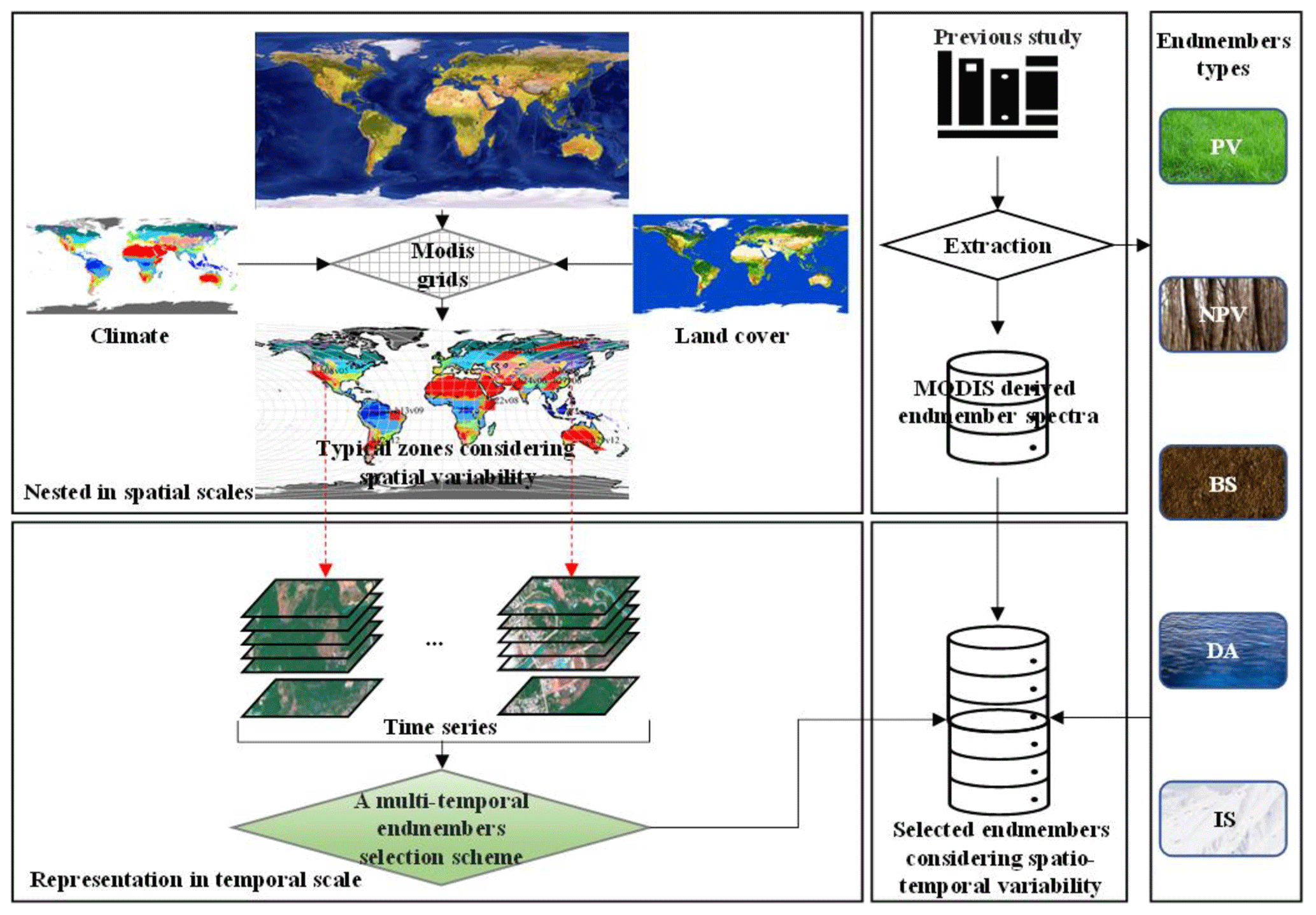
Figure 1 A framework for endmember selection considering spatial and temporal variability.

2.2.1 Nested endmember selection considering spatiotemporal variability

The quality of spectral mixture analysis is significantly dependent on the representativeness of the endmembers selected. Endmember spectra used in spectral mixture analysis, in general, can be derived from either a measured field spectral library or images (Franke et al., 2009; Sonnentag et al., 2007). The image-based endmember selection method is a more practical way because the advantage of image endmembers is that they can be collected at the same scale as the image and are relatively easy to associate with image features (Rashed et al., 2003). Given that such endmember selection would be hampered by the temporal and spatial variability of global intra-class and inter-class endmember spectra, we develop a nested framework for endmember selection considering spatial and temporal variability (Fig. 1).

1. Recent studies have proposed various compositional endmember frameworks in different application contexts. For example, a framework including substrate, vegetation, dark and ice or snow was proposed and verified globally for both Landsat and MODIS to allow estimated fractions. This framework ensures consistent comparison of estimated fractions across diverse climate patterns and land cover types (Small and Milesi, 2013; Sousa and Small, 2019). Another framework includes photosynthetic vegetation, nonphotosynthetic vegetation, soil and shade (Roberts et al., 1993). This framework was widely adopted for a presentation surface structure worldwide, particularly in tropical rainforest and dryland ecosystems (Guerschman et al., 2015). These elements can characterize the fundamental composition of Earth's surface. Thus, we use five endmembers to represent surface units, and these five endmembers include PV, NPV, BS, DA and IS. Concretely, PV refers to green photosynthetic foliage characterized by chlorophyll absorptions in the visible and high reflectance in the near-infrared bands; NPV represents non-tilled cropland or grassland and tree litters; and BS contains soil, rock and sediment. DA represents a fundamental ambiguity; thus, it may be either an absorptive (e.g., black lava), transmissive (e.g., deep clear water) or non-illuminated (shadow) surface. IS represents permanent glaciers and snow that are widespread in the polar regions and high mountains.

2. Considering both climate patterns and land cover types, the typical sites employed for standardized endmember selection were chosen based on the global MODIS sinusoidal grid (10° × 10° intervals). The Köppen–Geiger climate classification zones are adopted as the dominant criterion for undertaking full coverage of climate types (Beck et al., 2018). Meanwhile, we also examine the land cover diversity, characterized by Simpson's diversity index (D) of the recent MCD12Q1 Version 6 product in 2020 in each MODIS grid.

   $$\begin{array}{}\text{(3)}& D=\mathrm{1}-\sum _{i=\mathrm{1}}^m{\left(P_i\right)}^{\mathrm{2}}\end{array}$$

   P_i is the percentage of type i land use and cover in the grid, and m is the number of the land use and cover in the grid. Finally, we selected the top 10 grids (i.e., h08v05, h12v12, h13v09, h16v01, h21v03, h22v02, h22v08, h24v06, h26v05, h27v06 and h29v12) in terms of D among all the MODIS grids (Fig. S1a, b in the Supplement) and containing all the Köppen–Geiger climate types (Fig. S1c). These were selected for generation of the standardized endmember spectrum.

3. The representativeness of endmembers always shifts with the time variation. A multitemporal endmember selection scheme has been validated for various time series images (Sun and Liu, 2015; Sun et al., 2018). This process of utilization of both spatially and temporally mixed image collections for endmember selection can consider both spatial and temporal variability. Therefore, the multitemporal standardized endmember selection scheme is adopted in 10 typical zones that consider both climate and land cover diversity. Principal component (PC) transformation-derived eigenvectors and the associated PC images were utilized as criteria for determination of endmember types. Specifically, the eigenvector of the PC, displaying remarkable differences between shortwave infrared bands with other visible and near-infrared bands, is obviously able to highlight characteristics of IS. The PC eigenvector with a relatively high contrast between the near-infrared band and other bands primarily captures information related to PV, particularly during vegetation growing seasons. The BS and NPV will be boosted with the PC when the corresponding eigenvector emerges in the same direction. Even though there is no obvious regular pattern of the eigenvector for DA determination, the PC images can provide adequate information coupled with high-resolution images from Google Earth. After the determination of the endmember types and their PCs in each grid, we ranked these PCs by descending order of the variance contribution and selected PC images of the first three timings for endmember selection. We have listed the endmember types and their highlighted timings for each selected grid in Table S1 in the Supplement. The image endmembers can be acquired from the vertex's pixels (200–400 pixels) of the scatter plot formed by the PC images at their corresponding timings in each grid. We then exported these acquired pure pixels as regions of interest to compute the original MODIS reflectance as endmember spectra. These selected pure pixels for each endmember are validated by the high-spatial-resolution remote sensing imagery of Google Earth (Fig. S2).

4. In addition, we collect the MODIS-derived endmember spectra used in the previous study to complement and enrich the diversity of the spectral library (Okin et al., 2013; Daldegan et al., 2019; Meyer and Okin, 2015; Sousa and Small, 2019). We gather seven PV, five NPV, five BS and one DA endmember spectra through such a literature search method. Finally, we establish a library of endmember spectra considering spatiotemporal variability: this library includes 35 PV spectra, 40 BS spectra, 25 NPV spectra, 16 DA spectra and 15 IS spectra.

5. To ensure the feasibility of pixel-by-pixel operations in GEE, we also consider the similarity between the spectral curves. The hierarchical clustering method is selected to aggregate these spectra of each endmember as subgroups, and we input all spectral curves per endmember, grouping similar curves to compute their mean – a representative typical spectral curve for each cluster. Such hierarchical clustering boasts strong interpretability and adaptability for clustering at diverse scales within data analysis. Finally, we obtain four PV spectra, four BS spectra, three NPV spectra, two DA spectra and two IS spectra to estimate vegetation and soil fractions at the global scale from 2001 to 2020 (Fig. 2).

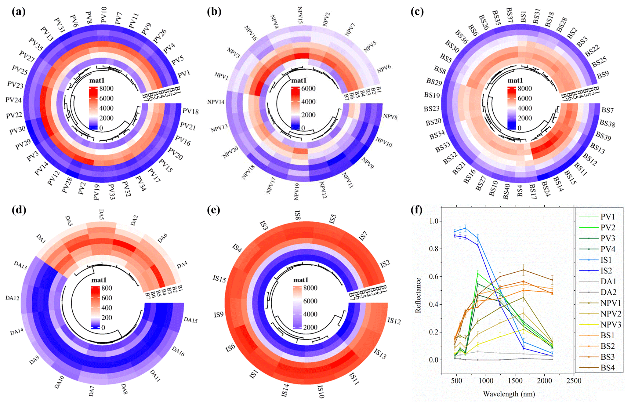
Figure 2 Endmember spectra. (a–e) Hierarchical clusters of the endmember spectra of PV, NPV, BS, DA and IS. (f) The averaged final endmember spectra, including four PV spectra, four BS spectra, three NPV spectra, two DA spectra and two IS spectra. B1–B7 represent MODIS spectral bands, including 459–479, 545–565, 620–670, 841–876, 1230–1250, 1628–1652 and 2105–2155 nm.

2.2.2 Multiple endmember spectral mixture analysis

MESMA has been used to estimate fractional vegetation–soil nexuses based on selected endmember spectra. According to the convex geometry concepts, the number of endmembers (n+1) in the model should be equal to the intrinsic dimensionality of the spectral space (n) plus 1 (Boardman, 1993). We found that the cumulative contribution of the top three PCs has exceeded 99 % (Fig. S3): this three-dimensional PC space allows four-endmember models. We initially generate multiple endmember combinations based on selected endmember spectra and achieve 692 combination models, including a two-endmember model (88), three-endmember model (252) and four-endmember model (352) (Table S2). The fully constrained least-squares spectral mixture analysis model is selected to estimate the fractions and count RMSE_sma for each endmember combination on the GEE platform. We finally search a specific endmember combination with the smallest RMSE_sma and achieve the estimated endmember fractions of this combination as the final fractions.

2.3 Direct validation of the dataset

The smallest RMSE_sma of 692 combination models is adopted as a criterion to assess the suitability and uncertainty of the model. The model suggests a generally good fit when the mean RMSE_sma over the image is less than 0.02 (Wu and Murray, 2003). Moreover, due to challenges in conducting fraction estimation validation through field surveys, we employ reference data obtained from high-spatial-resolution images as the validation set. We thus select for two sets of reference data where their land cover classification systems are closely related to our five endmembers. The Global Land Cover Validation Reference Dataset (GLCVRD) is provided with a 2 m reference dataset from very high-resolution commercial remote sensing data within 5 × 5 km blocks from 2003 to 2012 (Olofsson et al., 2012; Pengra et al., 2015; Stehman et al., 2012). These datasets support global estimates of the classification accuracy for the major land cover classes: tree, water, barren, other vegetation, cloud, shadow, ice and snow. Various recent studies have selected this dataset to evaluate the continuous fields of land cover types (Baumann et al., 2018; Qin et al., 2019; Song et al., 2018). We use all the GLCVRD reference datasets (Fig. 3a) to assess the accuracy of globally fractional vegetation and soil estimates from MESMA. Firstly, we filter the estimated fractions based on the corresponding year and month obtained from the reference data. Simultaneously, aligning the interpretations of land cover types with our endmembers, we pair them accordingly; i.e., tree and other vegetation represent PV and NPV, barren stands for BS, water and shadow correspond to DA, and ice and snow denote IS. Subsequently, we reclassify these paired land cover types and calculate their percentage within 5 × 5 km blocks, in which we exclude cloud coverage (named “no data”). Additionally, utilizing these cloud-free pixels in each block, we compute the mean of the fractional values for each endmember and then compare these estimated fractions with the measured percentage of paired reclassified land cover types to validate the reliability of our product (Fig. S4). Based on the paired measured fractions and our estimated fractions within blocks, we adopt four accuracy metrics, i.e., mean error (ME), mean absolute error (MAE), root-mean-square error (RMSE) and R² for accuracy assessment. ME measures the average of all the errors in the dataset where errors are the differences between predicted and actual values, MAE calculates the average of the absolute differences between predicted and actual values, RMSE provides a measure of the prediction error, and R² offers insight into the amount of variability in the dependent variable that the model explains. These metrics provide a more comprehensive assessment of the model's accuracy, helping to understand different facets of its performance, such as bias, variability and overall predictive power (James et al., 2013).

$$\begin{array}{}\text{(4)}& {\displaystyle }\mathrm{ME}={\displaystyle \frac{\sum _{i=\mathrm{1}}^n\left(p_i-r_i\right)}{n}}\text{(5)}& {\displaystyle }\mathrm{MAE}={\displaystyle \frac{\sum _{i=\mathrm{1}}^n\left|p_i-r_i\right|}{n}}\text{(6)}& {\displaystyle }\mathrm{RMSE}=\sqrt{{\displaystyle \frac{\sum _{i=\mathrm{1}}^n{\left(p_i-r_i\right)}^{\mathrm{2}}}{n}}}\text{(7)}& {\displaystyle }{R}^{\mathrm{2}}=\mathrm{1}-{\displaystyle \frac{\sum _{i=\mathrm{1}}^n{\left(p_i-r_i\right)}^{\mathrm{2}}}{\sum _{i=\mathrm{1}}^n{\left(p_i-\overline{r}\right)}^{\mathrm{2}}}}\end{array}$$

p_i and r_i are the estimated endmember fractions and reference endmember fractions at the ith block, n is the sample size (n=474), and $\overline{r}$ is the mean of the reference endmember fractions of all the blocks.

In addition, we also authenticate our product by incorporating comprehensive global land cover and land use reference data (Fritz et al., 2017), which were obtained from the Geo-Wiki crowdsourcing platform across four campaigns: human impact, wilderness, reference and disagreement. Over 150 000 samples of land cover and land use were acquired in these reference data. To effectively validate our product, we need to filter the reference data, considering aspects such as data acquisition time, measurement methods and credibility. We select the first three campaigns, which have a good match with MODIS pixels (size 1 × 1 km) and were observed from 2001 to 2022. High-feasibility reference data are then selected through the confidence information of land cover estimates and the status of use of high-spatial-resolution imagery provided by the metadata. Similarly to the procedural description used for fractional vegetation and soil compared with GLCVRD, we reclassify 10 classes of this dataset into our four groups of endmembers, i.e., (1) tree cover, shrub cover, herbaceous vegetation and grassland, cultivated and managed as well as the mosaic of cultivated and managed or natural vegetation to PV and NPV; (2) flooded land and wetland and open water to DA; (3) urban and barren to BS; and (4) snow and ice to IS. This involves comparing the measured percent of land cover with the mean of endmember fractions within the corresponding 1 × 1 km pixels.

2.4 Comparisons and uncertainty analysis

To verify the consistency and merits of our dataset against existing ones, we conducted comparisons with four distinct pre-existing datasets: the NDVI, the leaf area index (LAI), the MOD44B vegetation continuous-field product, the GLASS fractional vegetation cover dataset and the GEOV FCover dataset. The NDVI is derived from monthly synthesized MCD43A4 images. The LAI is derived from a 8 d composite MOD15A2H V6 dataset at 500 m resolution. Both mean values of the NDVI and LAI and our estimated fractional PV across all the years are considered for comparison. The MOD44B vegetation continuous-field product provides annual information about the percent tree cover, percent non-tree cover and percent non-vegetated within each 250 m pixel globally (DiMiceli et al., 2015). Consequently, we compare vegetation cover proportions – the sum of the percent tree cover and the percent non-tree cover – with the sum of the fractional PV and NPV. To align the spatial and temporal resolutions, we aggregated the sum of the percent tree cover and percent non-tree cover to a 500 m scale. Simultaneously, we computed the monthly fractional PV and NPV as annual averages. The GLASS fractional vegetation cover dataset, offering an 8 d temporal frequency and dual spatial resolutions of 0.05° and 500 m, was generated using a machine learning approach correlating MODIS reflectance with fractional vegetation cover (Jia et al., 2015). In our study, the 500 m GLASS data were utilized to validate our estimated fractions. We computed annual averages from all the GLASS fractional vegetation cover data within a year and compared them with the annual averages of the fractional PV and NPV. GEOV FCover is a 10 d product estimated through the neural network using the visible, near-infrared and shortwave infrared at 1 km resolution (Baret et al., 2013). We aggregate our product to a 1 km spatial resolution and compare their annual averages with the annual averages of GEOV FCover.

Moreover, we also carry out a comparison with traditional linear spectral mixture analysis to demonstrate the advantages of our spatiotemporally adaptive spectral mixture analysis. Such a comparison is performed using the average of the monthly RMSE_sma of the fully constrained framework based on two fixed endmember spectral curves: (1) the average of all the spectral spectra for each endmember and (2) the existing spectral spectra from Small and Sousa (2019).

Furthermore, to validate the uncertainties of the hierarchical clustering, we select a spectral spectrum from selected endmember spectra that exhibit the largest mean squared error from the mean of the cluster for each cluster. These selected spectral spectra were then used to reconstruct an extreme library of endmember spectra and were used to estimate the fractional vegetation and soil using MESMA.

2.5 Change in vegetation and soil fractions

A Mann–Kendall test is commonly referred to as a nonparametric test method, which is a procedure that detects monotonic trends of sequences over time (Kendall, 1975; Mann, 1945; Bradley, 1968). When seasonal environmental data of interest are available as time series for which the time intervals between adjacent observations are less than 1 year (i.e., daily, weekly and monthly sequences), a multivariate extension of the Mann–Kendall test has been advanced to handle seasonal sequences. In addition, the seasonal Sen slopes (change per unit of time) are commonly chosen to express this magnitude (Hirsch et al., 1982; Sen, 1968). Therefore, we impose the seasonal Mann–Kendall test and seasonal Sen method to define the trend and slope (annual change) of endmember fractions at the pixel level. The detailed information about the seasonal Mann–Kendall test and the seasonal Sen method can be found in the Supplement. If the Mann–Kendall test is not statistically significant (p≥0.05), we define the net change as 0. If the trend test is significant (p<0.05), we apply the seasonal Sen method to estimate the per-pixel net change between 2001 and 2022 (i.e., slope times of 22 years). In addition, we aggregate the per-pixel net change in endmember fractions to spatial scales (such as country, biome or climate zone) to obtain the total area change estimates at these aggregated scales from 2001–2022 as

$$\begin{array}{}\text{(8)}& \text{Net area change}=\sum _{i=\mathrm{1}}^n{T}_i{A}_{i}N,\end{array}$$

where T_i is Sen's slope of the endmember fraction for a statistically significant pixel i, A_i represents the area of pixel i, n is the total number of such pixels in the region, and N is the length of the study period (N=22).

3 Results

3.1 Evaluation of monthly estimates of vegetation and soil fractions

We utilize standard endmember spectra globally to estimate fractional vegetation–soil nexuses via MESMA. The simulated results elucidate that the MESMA model performs well with an ideal model RMSE_sma over the globe (0.018 ± 0.022, Fig. 3a–c). We find that the regions with RMSE_sma above 0.02 account for less than one-fifth of the global area and are mainly distributed in barren areas such as the Sahara and polar regions. This exceptional performance demonstrates the superiority and low uncertainty of the model. This performance is also evidenced by evaluation results from GLCVRD (Fig. 3e–h, Table S3). Specifically, the performance of PV + NPV, BS and IS endmember estimates have an MAE of less than 0.118, an RMSE of less than 0.149 and an R² of greater than 0.592. Although the MAE (0.050) and RMSE (0.065) perform well, the R² of the estimated DA against the measured DA represents only 0.156, largely attributed to the absence of estimations for shadows cast by smaller vegetation within the validation dataset. In blocks with a DA greater than 0.2, the estimated DA and measured DA present better consistency, in which the shadows of hills are well measured by GLCVRD. Moreover, we simultaneously select another set of land cover reference data as validation samples (Fig. S5). The validation results demonstrate the superiority of our estimation products, with the MAEs for PV, NPV, DA, BS and IS abundances all less than 0.099, the RMSEs all less than 0.129, and the R² values all greater than 0.57. However, this set of validation data is also not ideal as it fails to accurately estimate small-scale vegetation shadows and bare soil in highly vegetated areas, resulting in a slight overestimation of our DA and BS estimates near zero, accompanied by an underestimation of PV and NPV in high-value areas.

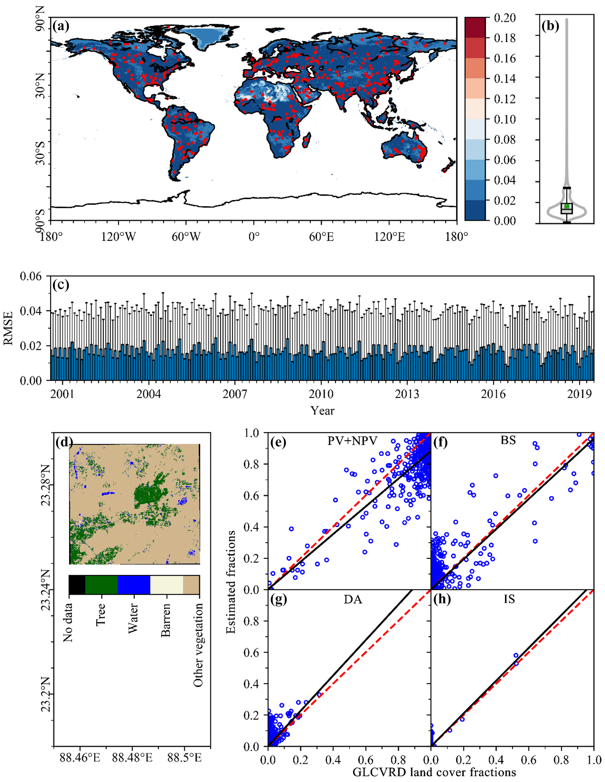
Figure 3 Evaluation of global fractional endmember estimates. (a) The spatial pattern of the average of the monthly RMSE_sma from 2001 to 2022; the overlaid red dots are the spatial distribution of the 5 × 5 km validation blocks of the GLCVRD reference dataset (n=500). (b) The boxplot and violin plot for the average of the monthly RMSE_sma (a), which indicate that the mean RMSE_sma over the image is less than 0.02. (c) The monthly averaged RMSE_sma from 2001 to 2022 with error bars. (d) The schematic of the detailed land cover classes of the GLCVRD reference dataset. (e–h) Scatter plots of the PV + NPV, BS, DA and IS fractions against the GLCVRD reference dataset (tree + other vegetation, barren, water + shadow, ice and snow). Endmember fractions were derived from the corresponding year and month of each 5 × 5 km block achieved.

3.2 Comparison with other datasets and the traditional spectral mixture analysis model

We compare our estimated vegetation and soil fraction dataset with the NDVI, fractional PV and NPV against fractional tree and non-tree vegetation of the MOD44B vegetation continuous-field product and other fractional vegetation cover products. We detected a strong positive relationship between the PV fraction and the NDVI. However, this correlation becomes less pronounced when PV exceeds 50 %, suggesting an evident saturation effect within the NDVI (Fig. 4a). This linear relationship also exists in the relationship between PV and the LAI, but a nonlinear turning point occurs when PV exceeds 70 % (Fig. 4c). Furthermore, the PV and NPV fraction displays a significant positive association with the remaining three fractional vegetation cover products (Fig. 4b, d, e). Specifically, the MOD44B vegetation continuous-field product reveals an R² of 0.75 with a p value below 0.01, the GLASS product displays an R² of 0.69 with a p value below 0.01, and the GEOV FCover product exhibits an R² of 0.65, also with a p value below 0.01. Nevertheless, within regions with lower vegetation cover, especially drylands that present a higher presence of nonphotosynthetic materials, the current products (particularly GLASS and GEOV FCover) have not adequately evaluated vegetation coverage, resulting in some degree of underestimation in the outcomes (Figs. 4c, d, S6a). Furthermore, we notice overestimation in the MOD44B vegetation continuous-field product in areas where vegetation cover is less than 50 %, mainly due to insufficient estimation of dark components (i.e., shadow of vegetation and mountains, water) (Figs. 4b, S6c). In areas with denser vegetation cover, we found good alignment among these products, especially with the MOD44B vegetation continuous-field product. However, the GLASS and GEOV FCover products tend to underestimate certain areas, primarily focusing more on green vegetation and overlooking nonphotosynthetic components (Figs. 4c, d, S6b). Moreover, both of the two fully constrained linear spectral mixture models are inferior to our framework since we consider the variability of the spectra in both time and space (Fig. 4e, f).

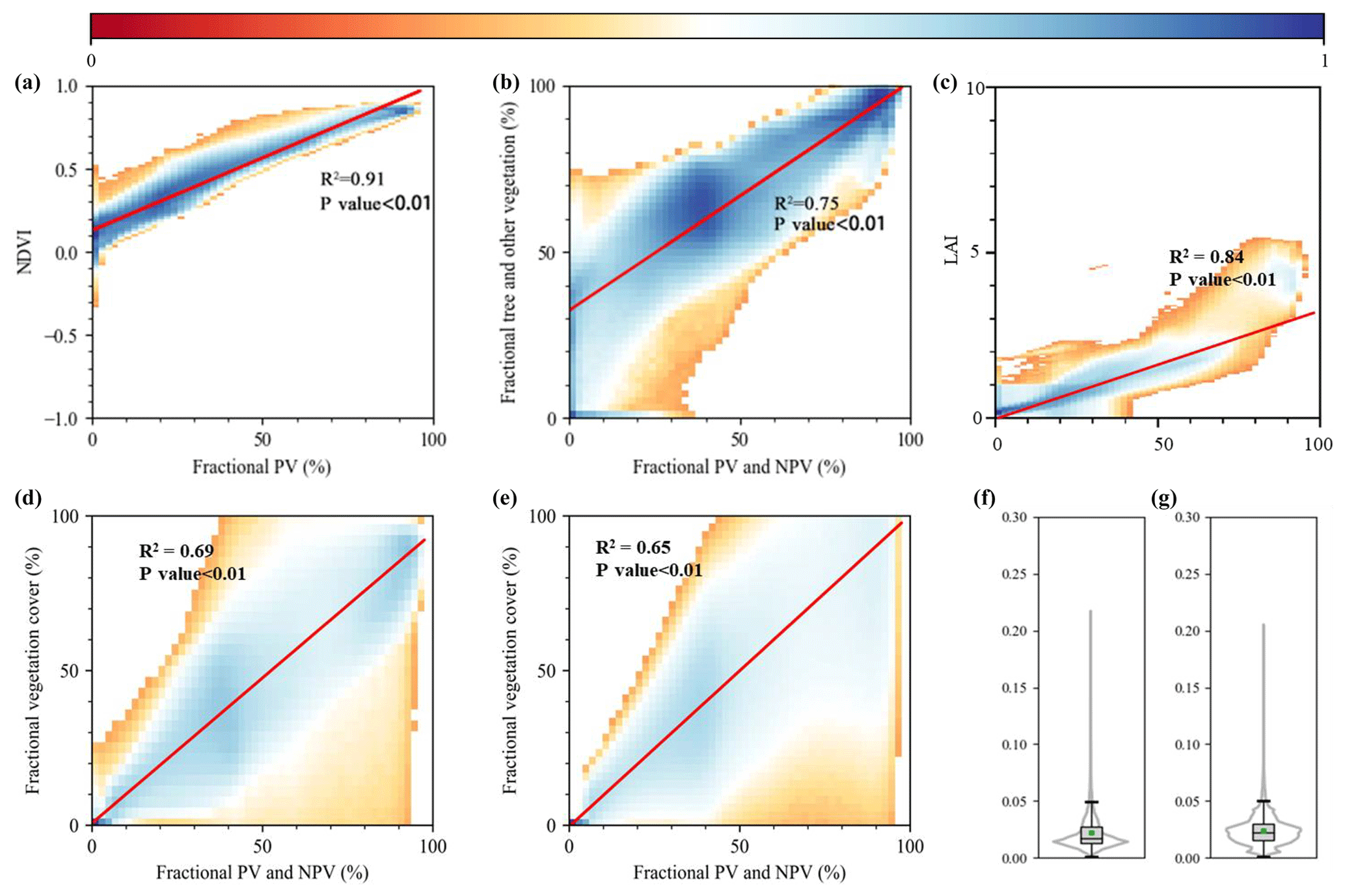
Figure 4 Comparisons with other datasets and traditional spectral mixture analysis models. (a–e) The bi-dimensional histogram of fractional endmembers and other datasets with a bin size of 2 %, including the fractional PV against NDVI (a), the fractional PV and NPV against the fractional tree and non-tree vegetation of the MOD44B vegetation continuous-field product (b), the fractional PV against the LAI (c), the fractional PV and NPV against the GLASS fractional vegetation cover product (d) and the fractional PV and NPV against the fractional vegetation cover of the GEOV FCover product (e). (f, g) The boxplot and violin plot for the average of the monthly RMSE_sma for two fixed endmember spectral curves using fully constrained linear spectral mixture models, including (e) the average of all the spectral spectra for each endmember and (f) existing spectral spectra from Sousa and Small (2019).

3.3 Uncertainties of estimates of global vegetation and soil fractions

It can be found that 90 % of the RMSE_sma's differences are concentrated within 1 % (Fig. 5a), indicating the relative stability of the unmixed results from the two libraries as well as the effectiveness of the clustering. These are also corroborated by the differences between the unmixed endmember fractions (Fig. 5b–e), as indicated by more than 90 % of the global pixels having a difference of 10 % or less as well as more than 70 % of the global pixels presenting a difference of up to 1 %, except for the two endmembers with higher spatial variability (NPV, 61.59 %; DA, 62.59 %).

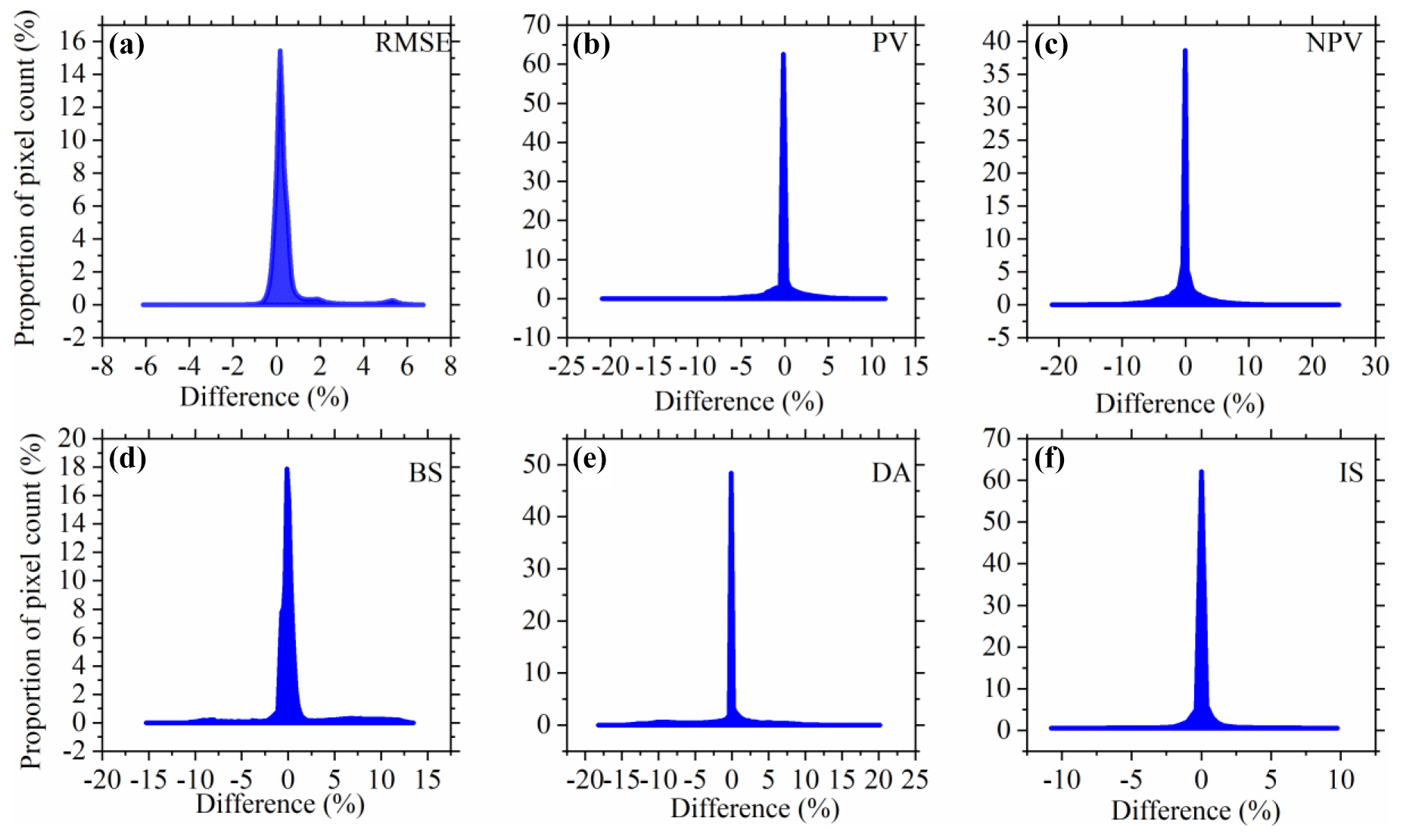
Figure 5 Difference in unmixed results between the mean endmember library and the extreme endmember library in the hierarchical cluster. Panels (a)–(f) represent the histogram of RMSE_sma, PV, NPV, BS, DA and IS.

3.4 Spatial distribution of global vegetation and soil fractions

Globally averaged monthly gradations of five surface vegetation and soil components are illustrated in Fig. 6. Our estimates show that PV cover presents the largest area for both 30–60° N and 0–30° S, which together account for more than half of the total global terrestrial vegetation area. We find that the average PV fraction in the Northern Hemisphere is significantly less than that in the Southern Hemisphere, especially in the Amazon, although the area of PV at 30–60° N is slightly greater than that of 0–30° S. Dominated by foliage-free desert vegetation and agricultural straw, NPV is mainly found in the semi-arid regions (e.g., USA, western China and Australia) and croplands. BS is also located in the drylands of the Sahara, western Asia and western–central Australia in terms of both fraction and total area. DA and IS, on the one hand, are mainly concentrated in terrestrial water bodies and mountains, Greenland and global high mountains of the Himalayas and Andes, respectively.

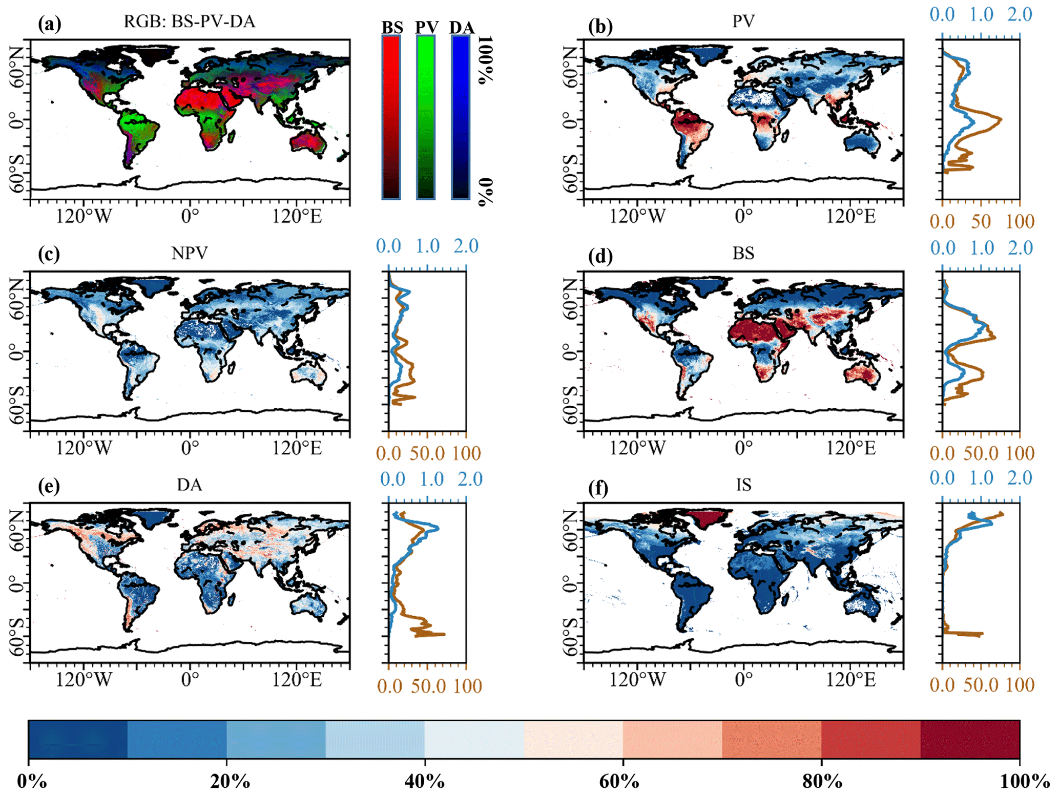
Figure 6 Global average of monthly fractional endmembers from 2001 to 2022. (a) Spatialized RGB composition of three averages of monthly fractional endmembers (RGB: BS–PV–DA). (b–f) Average of the PV, NPV, BS, DA and IS fractions. Shadowed subplots are the average of the fractional endmembers (%, orange, lower) and the area of endmembers (fraction × pixel area, ×10⁶ km², blue, upper) at the respective latitudes, taking each degree as the statistical standard.

3.5 Globally and regionally fractional endmember dynamics

The total area of PV increased by 9.35 × 10⁵ km² from 2001 to 2022, which represents a +1.88 % change relative to the 2001 green vegetation (Fig. 7; Table S4). This increased trend results from a higher magnitude of gain (1.57 × 10⁶ km²) nearly 2.5 times the loss area. Our PV area gain estimate basically agrees in magnitude with the global vegetation continuous-field product's estimate of net vegetation area change (1.36 × 10⁶ km²) despite differences in the time period covered (1982–2016) and definition (tree and other vegetation) (Song et al., 2018). Temperate, arid and cold regions together contribute more than 90 % of the greening area (Fig. 8; Table S4). In these areas, China and India are two major contributors (Fig. S7) through land use management like ecological afforestation and agricultural expansion (Chen et al., 2019). Within the Brazilian Amazon, we find a large area of PV loss (Fig. S7), which is also supported by estimates of forest cover and loss (Qin et al., 2019).

A decreasing trend is observed in NPV globally (2.19 × 10⁵ km²), representing a −1.45 % change relative to the 2001 NPV area (Fig. 7; Table S4). Tropical and temperate regions together contribute more than 80 % of the loss area of NPV, which may result from global-warming-induced tree greening. Although the arid area is a major source of NPV (2.75 × 10⁶ km² in 2001, 18.2 % of the global NPV area), the change area of NPV is only less than 10 000 km² (Fig. 8; Table S4).

In the context of the greening of the vegetation, the degree of BS is reduced by 5.14 × 10⁵ km² during the study period, indicating a −1.09 % change relative to the initial BS of 2001. The decreased global BS trend occurs in temperate, arid and cold regions, accounting for over 90 % of the net BS change area. In contrast, the tropical region appears to have an increasing trend (+1.22 × 10⁵ km²) and thus offsets the decline in BS in the rest of the regions (Fig. 8; Table S4). This outcome results from the forest-loss-induced soil exposure in the Brazilian Amazon and Southeast Asia (Fig. S7). Meanwhile, the total area of DA also represents a net change of −2.27 × 10⁵ km² from 2001 to 2022, which represents a −0.69 % change relative to the 2001 DA area. The largest negative contributions to the decreased global DA appear in cold (46.26 %) and arid (32.87 %) regions (Fig. 6; Table S4). We observed an increase of 2.46 × 10⁴ km² in IS globally, which represents a +0.11 % change relative to the 2001 IS. Such a positive trend mainly benefits from the increase in snow and ice in the cold regions, in which the net increase area is 1.5 times greater than the global net IS change (Fig. 8; Table S4). This is caused by the increase in snowfall. However, global warming is causing substantial melting of snow and ice, resulting in the arid, tropical, temperate and polar regions showing a decreasing trend in IS cover.

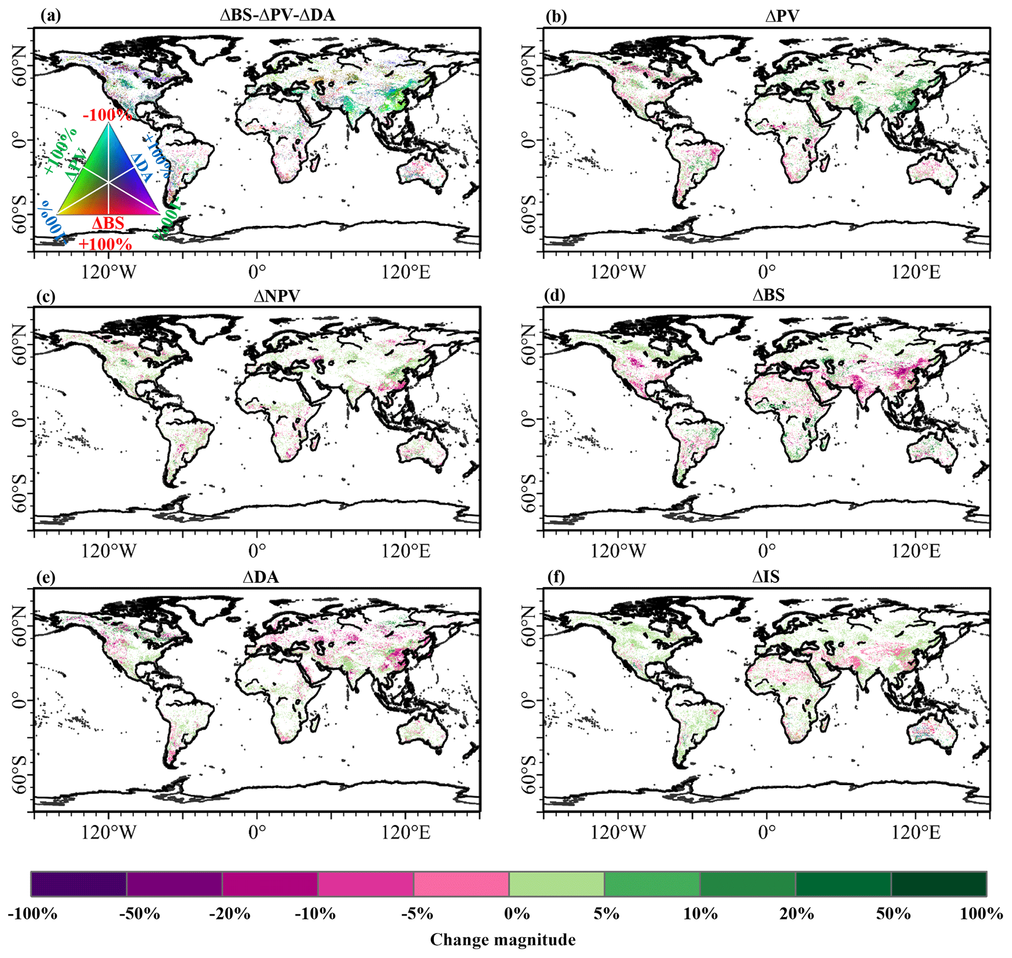
Figure 7 Globally fractional endmember dynamics at the pixel level. (a) Composited RGB image with ΔBS, ΔPV and ΔDA. (b–f) The change magnitude (%) in each pixel for the estimated endmembers, i.e., ΔPV, ΔNVP, ΔBS, ΔDA and ΔIS. Pixels showing a statistically significant trend (seasonal Mann–Kendall test, P<0.05) for either endmember are depicted on the change map.

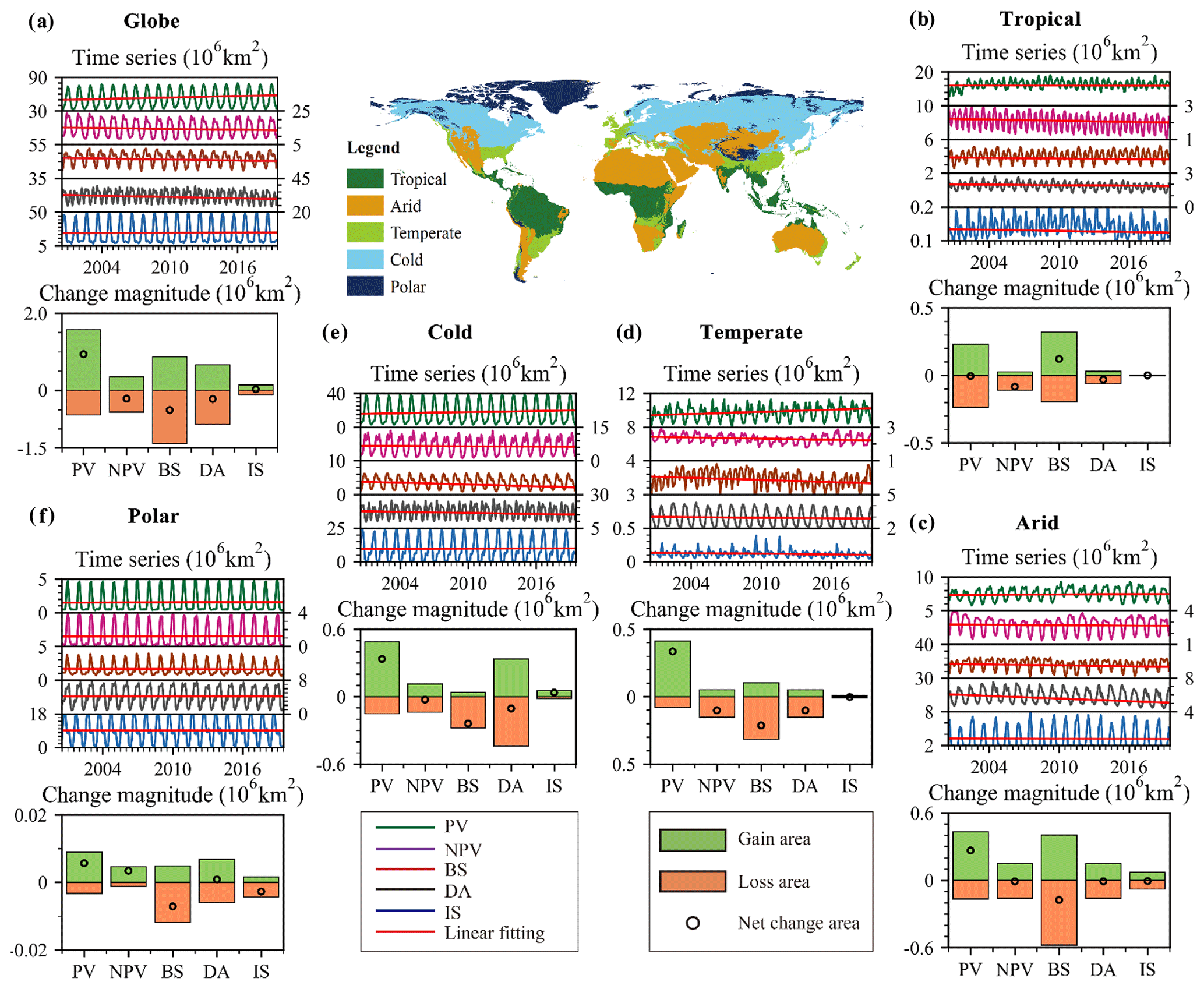
Figure 8 Global and regional fractional endmember dynamics. The middle subgraph is aggregated into five Köppen–Geiger climate classes. (a–f) The gain area, loss area and net change area for the five land surface endmembers in the globe (a) and the five climate zones, i.e., tropical (b), arid (c), temperate (d), cold (e) and polar (f).

4 Discussions

4.1 Advances and limitations of estimates of global vegetation and soil fractions

This paper implements global monthly estimates of fractional vegetation–soil nexuses in 2001–2022 via the high-accuracy and time-consuming MESMA algorithm at the subpixel scale (Roberts et al., 1998), benefitting from the GEE platform that can provide powerful computational processing to realize planetary-scale analysis of geospatial data. We can more conveniently target the most optimal model from 692 combination models for each MODIS pixel (500 m), thus helping to understand the specific vegetation–soil compositional structures in each pixel or region. Such a scheme can improve ecologists' and managers' understanding of multifaceted terrestrial ecosystems for differentiated measures. Moreover, these fractional endmembers have proven their potential for application in land use cover classification (Sun et al., 2020), time series evolutionary pathways (Sun et al., 2021; Daldegan et al., 2019) and biophysical process modeling (Sun et al., 2022; Sousa and Small, 2018). This globally comprehensive record of monthly vegetation and soil fractions during the period 2001–2022 may provide basic data for quantification and modeling of global change and provide an important foundation for measuring sustainable development goals such as land degradation neutrality (Chasek et al., 2018; Sun et al., 2019).

Our product can overcome the problem of saturation of the NDVI in the regions embodying high-coverage vegetation. Such an advance can be supported by previous regional comparison research (Rogan et al., 2002; Sun et al., 2019, 2020). Additionally, the diversity of information stands as one of the strengths of this dataset, encompassing the five primary components of Earth's land surface globally. Moreover, it can be extended to encompass more types through different levels of clustering. For instance, the DA component has not been emphasized in many datasets, yet current scientific research underscores the need for increased attention to vegetation shadows (Zeng et al., 2023). Although our DA component represents various types across different land regions, such as water bodies, shadows or bare rocks, this dataset may effectively enhance our precise understanding of complex vegetation structures. The NPV component is a vital element in arid ecosystems and represents a crucial part of vegetation biomass. Our dataset, by finely characterizing NPV, not only aids in understanding the evolving features of vegetation structure under photosynthetic and nonphotosynthetic interactions (Guerschman et al., 2015) but also contributes to a more accurate quantification of global biomass in arid land systems (Smith et al., 2019).

Moreover, our product demonstrates good scalability in terms of time and endmember types. These monthly estimates of fractional vegetation–soil nexuses can be upgraded to multi-timescale (daily, yearly) products to serve different needs and thus provide time series of multicomponent information on surface heterogeneous composition and interactive evolution. In addition, considering the meaningful physical interpretations of endmember fraction values, these endmembers can be conveniently integrated across different temporal and spatial scales using spatiotemporal fusion methods (Zhang et al., 2018). The temporal and spatial variability of endmembers has always been a significant constraint in obtaining global-scale vegetation and soil fractions from imagery (Wang et al., 2021). The spatiotemporally adaptive framework employed helps to increase the representativeness of endmember selection, and MESMA also considers the suitability of each combination of these endmembers within each pixel. However, considering the limitations of the computational resources, our solution on hierarchical clusters of the endmember spectra can considerably improve cost-effective unmixing of long time series satellite records over the globe under the tradeoffs of certain accuracy requirements (Fig. 3). With the assumption of increased computational power in the future, we believe that utilization of combination models from selected endmember spectra (35 GV spectra, 40 BS spectra, 25 NPV spectra, 16 DA spectra and 15 IS spectra) or expanded endmember spectra may further improve the accuracy and stability of estimates of gradations of five surface vegetation and soil components at the global scale.

However, due to the absence of corresponding reference data for validation, we solely rely on two high-quality land cover reference datasets for validation. Unfortunately, these datasets do not intricately characterize small-scale shadows and bare soil within complex vegetation structures. Consequently, this leads to a misconception in the validation, where our DA and BS are overestimated in low-value areas and vegetation is underestimated in high-value areas (Figs. 3, S5). Therefore, in the future, there is a need to further develop high-quality relevant reference data. Considering that the MOD44B vegetation continuous-field product provides a gradation of three surface cover components, i.e., percent tree cover, percent non-tree cover and percent bare, the dark components (i.e., shadow of vegetation and mountain, water) are not quantified. Therefore, the fractional PV and NPV are overall biased high, especially in areas with PV and NPV less than 0.50 (Figs. 4b, S6b). In addition, we also observed a certain degree of underestimation in these three datasets in regions with lower vegetation cover compared to our data. This is mainly because these datasets focus solely on green vegetation, especially GLASS and GEOV FCover (Baret et al., 2013; Jia et al., 2015), and do not accurately estimate nonphotosynthetic vegetation in arid regions. The above comparisons demonstrate our precision advantage in fine extraction of multiple endmembers. Given the importance of NPV in ecological research, undertaking separate validation and comparisons between PV and NPV represents a critical foundational effort. While detailed maps of a representative region illustrate the reliability and advantages of our NPV estimation over other products (Fig. S6), the current lack of equivalent products highlights the need for ongoing development. Enhancing quantitative comparison efforts will be essential for bolstering the feasibility, accuracy and validity of our NPV product in future studies. We observed higher RMSE_sma values in seemingly homogeneous areas like the Sahara and Arctic. However, within these regions, there often exist extremely diverse land cover types, such as high- and low-reflectance sands and ice. When selecting endmembers and hierarchical clustering models, we might not have adequately considered these extreme spectral curves. As a result, these extreme areas exhibit a higher uncertainty.

4.2 Implications of global and regional shifts from pairs of two endmembers

We find greening of Earth characterized by increased photosynthetic vegetation and reduced bare soil exposure, observed in temperate and cold countries such as Russia (Figs. 9, S3). This finding is in agreement with the finding of a climate-driven greening trend in the Northern Hemisphere (Piao et al., 2006). The biomass decreases, exhibited as decreased PV and increased BS (Fig. 9), presented only half of the global climate-driven greening. These findings imply a global trend towards greening in the context of global warming, as supported by a large number of published studies on global vegetation change (Chen et al., 2019; Piao et al., 2006; Song et al., 2018). Moreover, the polar zone is a hotspot of ice melting and shows the accepted fact of accelerated retreat of glaciers and ice under global warming (Hugonnet et al., 2021; Zemp et al., 2019).

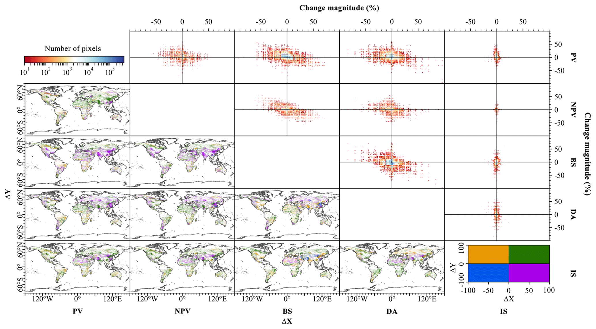
Figure 9 Characteristics of each pair of two endmembers. The bottom-left corner shows global maps of co-location of two paired endmembers. Pixels showing a statistically significant trend (seasonal Mann–Kendall test, P<0.05) in both endmembers are depicted on the map. The color of each pixel was displayed in quadrants of ΔX and ΔY, where ΔX and ΔY are horizontal and vertical endmembers, respectively. The top-right corner shows a two-dimensional histogram of the change magnitude (%) of the two paired endmembers. The x axes and y axes are represented by ΔX and ΔY, respectively. These two-dimensional histogram plots were created with a bin size of 1 % for both axes. The color bar was normalized by the number of pixels in each bin on a log scale.

In addition, the overexploitation of resources is one of the environmental problems of interest and an important factor in causing the above climate change and disasters. Global overexploitation has led to problems such as vegetation degradation and intensive utilization of agricultural land. The human overexploitation of forest- and grassland-induced biomass decrease presents a decrease in PV and an increase in BS (Figs. 9, S7), especially over the tropical rainforest of the Brazilian Amazon and South Asia. This finding agrees with the deforestation and agriculturalization in these regions provided by previous studies (Qin et al., 2019; Zhen et al., 2018). Within the agricultural area, the agricultural intensification is a human-driven greening process characterized by increased photosynthetic vegetation and reduced bare soil. This shift mainly occurs in India and the North and Northeast China Plain (Figs. 9, S7) (Chen et al., 2019). We also found an urbanization-driven biomass decrease in the global terrestrial ecosystems, especially in China and North America (Figs. 9, S7), resulting from occupation of agricultural and ecological lands during urban sprawl (Kuang et al., 2020, 2021; Zhao et al., 2022).

Eco-restoration depicts a process that currently needs urgent attention in our understanding and utilization of resources and the environment. Differently from climate-driven greening that presents trends of increasing PV and decreasing BS, the human-driven afforestation shows positive trends of both PV and NPV, mainly attributed to recent implementation of policies on ecological restoration through a large number of planted protective forests (Figs. 9, S7). These afforested regions are primarily found over China, Europe and North America, supported by a previous study on the greening world (Chen et al., 2019). Moreover, green space construction in urbanized regions has been carried out, integrated with road construction and city renovation, and generates an increasing footprint of urban greening, especially in China (Figs. 9, S7).

This dataset can serve as a baseline for enhancing our comprehension of heterogeneous surface dynamics and modeling Earth's biophysical processes through a multi-endmember coupling perspective and may significantly advance future research by serving as a foundational reference for delving deeper into complex land systems. Anticipating its potential applications across diverse domains such as ecology, climate studies and urban planning, this dataset emerges as a pivotal resource. Its multifaceted utility is expected to play a pivotal role in informing environmental management decisions, advancing studies on ecological shifts, predicting climate trends and facilitating strategic landscape planning.

5 Data availability

The data about the fractional five surface vegetation and soil components can be exported from the GEE platform via the provided codes or are available in the Science Data Bank (https://doi.org/10.57760/sciencedb.13287, Sun and Sun, 2023). The first dataset includes five fractions from 2001 to 2011, and another includes five fractions from 2012 to 2022. The file contains compressed month-by-month GeoTIFF data for each year according to the grid of longitude 60° and latitude 50°. The dataset for each year includes 216 files, named “SMA_year_(month-1)_gridid.tif”, like “SMA_2001_0_0.tif”. The public datasets have been listed in the Methods section.

6 Code availability

The GEE codes for MESMA and the seasonal Mann–Kendall test are available at GitHub (https://github.com/qiangsunpingzh/GEE_mesma, last access: 11 March 2024) and Zenodo (https://doi.org/10.5281/zenodo.10796386, Sun, 2024). Common code for generating figures is available at https://doi.org/10.5281/zenodo.10669804 (Caswell et al., 2024).

7 Conclusions

In this paper, to provide locally detailed socio-ecological knowledge about globally multifaceted changes in fractional vegetation–soil nexuses under climate change and anthropogenic impacts, we estimated monthly vegetation and soil fractions in 2001–2022 that provide multicomponent information on surface heterogeneous composition based on a spatiotemporally adaptive spectral mixture analysis framework. This product of monthly vegetation and soil fractions from 692 combination models can provide an accurate estimate of surface heterogeneous composition, better than the previous vegetation index and vegetation continuous-field product, as well as traditional fully constrained linear spectral mixture models. This solution can both improve considerably cost-effective unmixing of long time series satellite records over the globe and meet accuracy requirements. Based on these estimates of vegetation and soil fractions, we find a greening trend of Earth, as indicated by a increase in the total area of PV, which represents a +1.88 % change relative to the 2001 green vegetation. This greening trend can be found in all climatic zones other than the tropics. In addition to the trends in greening reported by other studies, we found that the increase in PV was accompanied by a decreasing trend in BS, DA and NPV in most regions. There is a trend of simultaneous increase in PV and NPV in central and southwestern China during afforestation activities. Therefore, a combination between interactive changes in vegetation and soil fractions can be adopted as a valuable measurement of climate change and anthropogenic impacts.