Global marine gravity gradient tensor inverted from altimetry-derived deflections of the vertical: CUGB2023GRAD

Geodetic applications of altimetry have largely been inversions of gravity anomaly. Previous studies of Earth's gravity gradient tensor mostly presented only the vertical gravity gradient (VGG). However, there are six unique signals that constitute the gravity gradient tensor. Gravity gradients are signals suitable for detecting short-wavelength topographic and tectonic features. They are derived from double differentiation of the disturbing potential and hence are susceptible to noise amplification which was exacerbated by low across-track resolution of altimetry data in the past. However, current generation of altimetry observations have improved spatial resolutions, with some better than 5 km. Therefore, this study takes advantage of current high-resolution altimetry datasets to present CUGB2023GRAD, a global (latitudinal limits of ±80°) 1 arcmin model of Earth's gravity gradient tensor over the oceans using deflections of the vertical as inputs in the wavenumber domain. The results are first assessed via Laplace's equation, whereby the resultant residual gradient is virtually zero everywhere. Further analysis at local regions in the Arctic and south Indian oceans showed that T_xy, T_xz and T_yz are the most dominant gravity gradients for bathymetric studies. This proves that bathymetric signatures in the non-diagonal tensor components are worth exploiting. Bathymetric coherence analysis of T_zz over the Tonga Trench showed strong correlation with multibeam shipboard depths. This study proves that current generation of altimetry geodetic missions can effectively resolve Earth's gravity gradient tensor. The CUGB2023GRAD model data can be freely accessed at https://doi.org/10.5281/zenodo.10511125 (Annan et al., 2024).

1 Introduction

It is now 50 years since Skylab, the first satellite altimetry mission, was launched in 1973. This was shortly followed by the GEOS-3 (Geodynamic Experimental Ocean Satellite) and Seasat missions, which spanned 1975–1979 and 1978, respectively. Satellites following these first-generation missions have shown improvements on the knowledge acquired and reflect improvements in the technologies developed during the lifespans of their respective predecessors (Escudier et al., 2018).

Developments in satellite altimetry over the years – such as the improved range accuracy from the Ka-band of SARAL/AltiKa – have resulted in more accurate sea surface heights (SSHs) (Verron et al., 2021, 2018). This and better spatial resolution and other advancements from the Ku-band missions (i.e., the Jason series, HY-2 series, Cryosat-2, Sentinel series and the recently launched SWOT mission) have enabled diverse applications of satellite altimetry in geodesy, geophysics, glaciology, oceanography and hydrology.

Marine gravity field recovery is the commonest geodetic application of satellite altimetry. Marine gravimetry is important for submarine navigation (Wan and Yu, 2014), delineating continent–ocean margins (Sandwell et al., 2013), exploring offshore energy resources (Becker et al., 2009), revealing submarine tectonic features buried by sediments (Hwang and Chang, 2014; Sandwell et al., 2014; Harper et al., 2021; Sandwell and Smith, 2009) and deep-sea bathymetry inversion (Annan and Wan, 2020, 2022; Wan et al., 2022).

For an altimetry satellite's observations to be considered for gravity field recovery, the observations ought to have been acquired during the geodetic mission (GM) phase of the satellite (i.e., in a long repeat orbit). Most satellites begin life in the exact repeat mission (ERM) phase, where they repetitively observe the same tracks of ocean surface in a short period, resulting in better temporal resolution at the expense of spatial resolution. The GM phase is usually considered the end-of-life of the satellite although some altimetry missions' GM phase is the start or middle phase of the satellite; this yields higher across-track spatial resolution at the expense of temporal resolution. The higher across-track spatial resolution enables the mapping of short-wavelength features in the gravity field (Andersen, 2013; Andersen et al., 2021). It helps to map out finer details of mean sea surface (MSS), which is used to improve sea level anomalies for the ERM, whereas the GM phase also benefits from long-term MSS modeled through the ERM phase. The MSS is used to reduce SSH measurements from the GM phase to obtain the geoid – the surface of equilibrium potential. A description of these two satellite phases is presented well in Andersen et al. (2021).

Although the geoid is the base gravity field signal recovered through satellite altimetry, it is sensitive to long-wavelength features. Conversely, short-wavelength features, which are of more interest to researchers, are better revealed through derivatives (i.e., deflections of the vertical, gravity anomaly and gravity gradient tensor) of the disturbing potential. Deflections of the vertical and gravity anomaly can be computed as first-order derivatives of the disturbing potential in the horizontal and vertical directions, respectively. Gravity gradients are the second-order derivatives and are better at revealing bathymetric and tectonic signatures. Gravity anomalies and gravity gradients can be recovered from geoid heights directly (i.e., through the inverse Stokes formula and double differentiation) or from deflections of the vertical (i.e., through the inverse Vening Meinesz formula and Laplace's equation). Previous studies have indicated that the use of deflections of the vertical is more accurate as it minimizes long-wavelength errors (Olgiati et al., 1995; Andersen, 2013).

Even though there are numerous studies about Earth's marine gravity field, most of them are focused on gravity anomaly and, to some degree, on deflections of the vertical. Studies in which gravity gradients have been studied usually discuss only the vertical component (often denoted as T_zz) of the gradient tensor although the tensor comprises six unique components. It suffices to conclude that more research has been conducted on marine gravity anomaly and its vertical derivative than full tensor of gravity gradients. Evidently, only Scripps Institution of Oceanography (SIO) releases publicly available gravity gradient models; even these are models of T_zz only. One of the reasons for the limited literature on marine gravity gradient tensors is that methods for inverting them from altimetry data are comparatively few, unlike those for inverting gravity anomaly. Another significant justification for this has been the low spatial resolution of altimetry observations in the past. This is because higher differentiation of the disturbing potential results in amplification of high frequencies, which unfortunately includes noise in the signal (Sideris, 2016; Bouman et al., 2011; Wan et al., 2023). However, current datasets from the GMs of Jason-1, Jason-2, HY-2A, SARAL/AltiKa and Cryosat-2 are more accurate and densified enough to instigate a revisit to altimetry-derived full tensor of gravity gradients. Generally, observations with 8 km across-track spatial resolution are deemed acceptable for gravity field recovery. With the exception of SARAL/AltiKa, which has variable across-track spatial resolution (i.e., 1–15 km) due to its drifting phase (Verron et al., 2021), the spatial resolutions of these other satellites are all better than 8 km (Andersen et al., 2021; Annan and Wan, 2021).

Therefore, this study takes advantage of the abovementioned highly densified datasets to develop CUGB2023GRAD (Annan et al., 2024), a global marine gravity gradients product consisting of all six components of the tensor. We compute the gravity gradients in the wavenumber domain through the remove–compute–restore method by using the north–south and east–west components of deflections of the vertical as input signals.

2 Datasets

This study uses the deflections of the vertical (east_32.1.nc and north_32.1.nc) developed by Scripps Institution of Oceanography (SIO: https://topex.ucsd.edu/pub/global_grav_1min/, last access: 1 February 2023) and deflections of the vertical we inverted from DTU21GRA – a highly accurate gravity anomaly model developed by Technical University of Denmark (DTU: https://ftp.space.dtu.dk/pub/DTU21/1_MIN/, last access: 24 February 2023). The DTU21GRA-derived deflections of the vertical were computed in a remove–compute–restore manner using Eq. (31) of Sideris (2016). The latest version of SIO's deflections of the vertical is an improvement of earlier models, which featured datasets from long repeat orbits (or geodetic missions) of SARAL/AltiKa, Cryosat-2, Jason-1/2 and Geosat satellites (Sandwell et al., 2019). It also incorporated 12-month additional datasets from Sentinel-3A/B, Cryosat SAR, Cryosat LRM and SARAL/AltiKa. Similarly, DTU21GRA also features datasets from SARAL/AltiKa, Cryosat-2 and Jason-1/2 (Andersen et al., 2023). The averages of these two sets of deflections of the vertical were computed as input for the inversion of the gravity gradient tensor.

The remove–compute–restore approach demands the removal of long wavelengths in the form of an initial gravity signal (i.e., deflections of the vertical). It is later restored in the form of the desired signal (i.e., gravity gradient tensor) after computations. To this end, the global geopotential model EGM2008 (Pavlis et al., 2012) was used to construct the required reference gravity signals. EGM2008 was obtained as spherical harmonic coefficients from the International Centre for Global Earth Models (ICGEM: http://icgem.gfz-potsdam.de/, last access: 1 February 2023). We used EGM2008 because it is the most widely used global geopotential model for studies involving marine gravity field (Sandwell et al., 2019; Zhang et al., 2017; Zhu et al., 2020, 2019; Andersen and Knudsen, 2019). The reference signals were simulated at a maximum degree of 2190 using the GrafLab program developed by Bucha and Janák (2013).

3 Derivation of gravity gradient tensor

Marine gravity gradient tensor is derived from the second-order differentiation of the disturbing potential in the horizontal and vertical directions. It is a tensor with nine components, of which three are redundant; therefore, there are six unique tensor components. The gravity gradient tensor in the local north-oriented reference frame is defined as (Petrovskaya and Vershkov, 2006; Bouman et al., 2011)

$$\begin{array}{}\text{(1)}& \left.\begin{array}{l}{T}_{xx}=\frac{T_{\mathit{\phi }\mathit{\phi }}}{r^{\mathrm{2}}}+\frac{T_{\mathrm{r}}}{r}\\ T_{yy}=\frac{T_{\mathit{\lambda }\mathit{\lambda }}}{r^{\mathrm{2}}{\sin }^{\mathrm{2}}\mathit{\phi }}+\frac{T_{\mathit{\phi }}}{r^{\mathrm{2}}\tan \mathit{\phi }}+\frac{T_{\mathrm{r}}}{r}\\ T_{zz}=T_{\mathrm{r}r}\\ T_{xy}=\frac{T_{\mathit{\lambda }\mathit{\phi }}}{r^{\mathrm{2}}\sin \mathit{\phi }}-\frac{T_{\mathit{\lambda }}\cos \mathit{\phi }}{r^{\mathrm{2}}{\sin }^{\mathrm{2}}\mathit{\phi }}\\ T_{xz}=\frac{T_{\mathit{\phi }}}{r^{\mathrm{2}}}-\frac{T_{\mathit{\phi }r}}{r}\\ T_{yz}=\frac{T_{\mathit{\lambda }}}{r^{\mathrm{2}}\sin \mathit{\phi }}-\frac{T_{\mathit{\lambda }r}}{r\sin \mathit{\phi }}\end{array}\right\}.\end{array}$$

T is the disturbing potential, which according to the Bruns formula, is related to the geoid, N, via the normal gravity in geoid, γ; i.e., T=γN. r is the mean radius of Earth, λ is longitude and φ is colatitude. $\left(x,y,z\right)$ is the coordinate in the local reference frame. x points in the latitudinal direction towards north, y points in the longitudinal direction towards west and z points in the radial direction outside of Earth.

Figure 1 Illustration of the remove–compute–restore approach used.

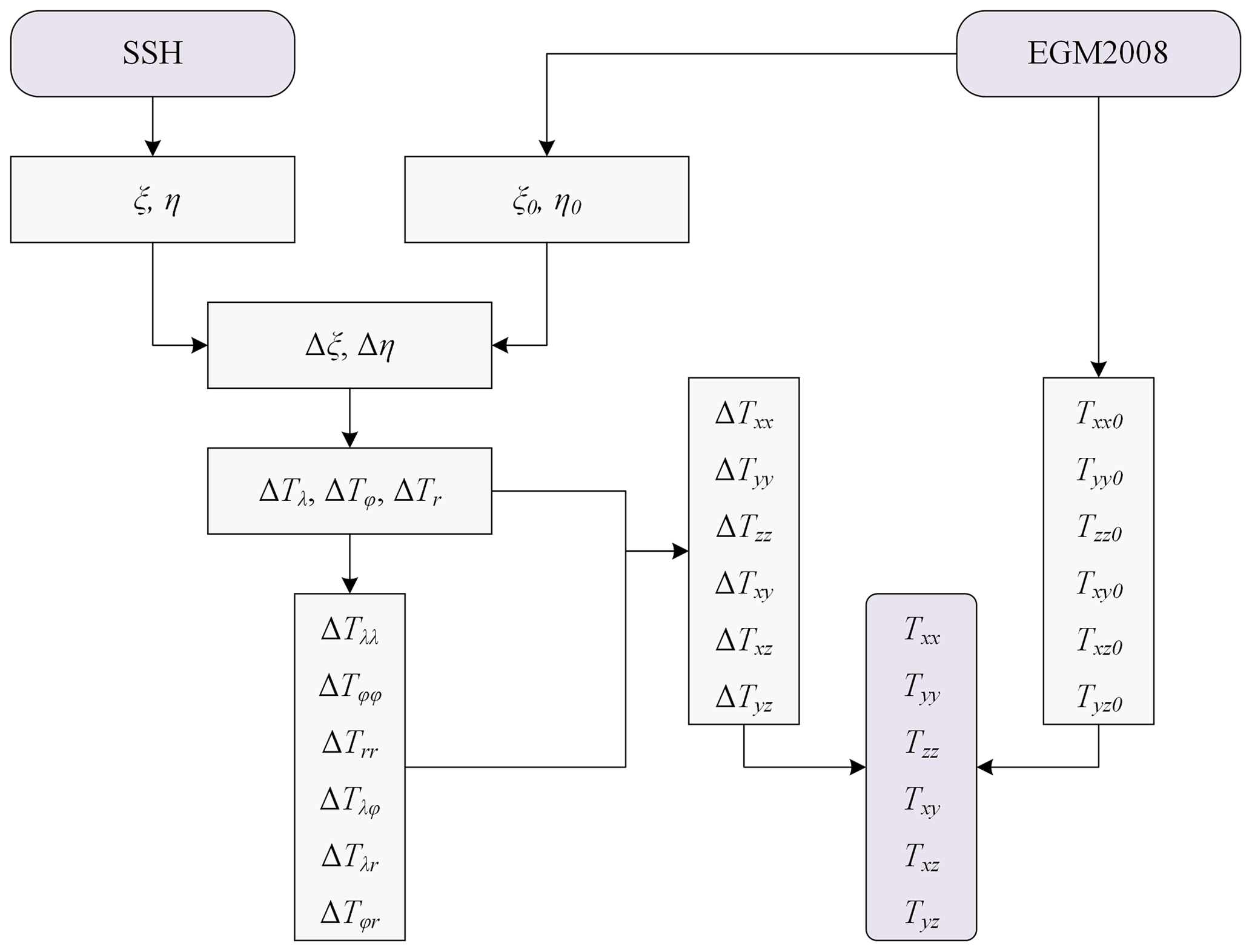
In order to implement the remove–compute–restore approach as illustrated in Fig. 1, we compute the residual components of deflections of the vertical, Δξ and Δη, by subtracting reference ξ and η derived from EGM2008, from the altimetry-derived ξ and η.

The relationship between components of deflections of the vertical and T can be expressed as

$$\begin{array}{}\text{(2)}& \left.\begin{array}{l}\mathit{\xi }=-\frac{\mathrm{1}}{\mathit{\gamma }r}\cdot \frac{\partial T}{\partial \mathit{\phi }}\\ \mathit{\eta }=-\frac{\mathrm{1}}{\mathit{\gamma }r\sin \mathit{\phi }}\cdot \frac{\partial T}{\partial \mathit{\lambda }}\end{array}\right\}.\end{array}$$

Therefore, using residual components of deflections of the vertical, it is obvious to infer from Eq. (2) that

$$\begin{array}{}\text{(3)}& \left.\begin{array}{l}\frac{\partial \mathrm{\Delta }T}{\partial \mathit{\phi }}=\mathrm{\Delta }{T}_{\mathit{\phi }}=-\mathrm{\Delta }\mathit{\xi }\cdot \mathit{\gamma }\cdot r\\ \frac{\partial \mathrm{\Delta }T}{\partial \mathit{\lambda }}=\mathrm{\Delta }{T}_{\mathit{\lambda }}=-\mathrm{\Delta }\mathit{\eta }\cdot \mathit{\gamma }\cdot r\sin \mathit{\phi }\end{array}\right\}.\end{array}$$

The first derivative of T in the vertical direction produces the radial disturbing gravity gradient, T_r. Its residual form, ΔT_r, is computed in the wavenumber domain using the residual components of deflections of the vertical as inputs.

$$\begin{array}{}\text{(4)}& \mathrm{\Delta }{T}_{\mathrm{r}}={\mathbf{F}}^{-\mathrm{1}}\left\{-{\displaystyle \frac{i\mathit{\gamma }}{k}}\left(k_x\mathbf{F}\left\{\mathrm{\Delta }\mathit{\xi }\right\}+k_y\mathbf{F}\left\{\mathrm{\Delta }\mathit{\eta }\right\}\right)\right\},\end{array}$$

where γ is the normal gravity. $k=\sqrt{k_x^{\mathrm{2}}+k_y^{\mathrm{2}}}$ such that k_x and k_y are defined as $\frac{\mathrm{1}}{{\mathit{\lambda }}_x}$ and $\frac{\mathrm{1}}{{\mathit{\lambda }}_y}$, respectively; λ_x and λ_y are the wavelengths in the horizontal direction. F and F⁻¹ are the Fourier transform and inverse Fourier transform, respectively.

Having computed the residual signals ΔT_λ, ΔT_φ and ΔT_r from Eqs. (3) and (4), the derivative property of the Fourier transform is then applied on them to obtain (Wan et al., 2023)

$$\begin{array}{}\text{(5)}& \left.\begin{array}{l}\mathrm{\Delta }{T}_{\mathit{\lambda }\mathit{\lambda }}={\mathbf{F}}^{-\mathrm{1}}\left\{i\mathrm{2}\mathit{\pi }{k}_y\mathbf{F}\left\{\mathrm{\Delta }{T}_{\mathit{\lambda }}\right\}\right\}\\ \mathrm{\Delta }{T}_{\mathit{\phi }\mathit{\phi }}={\mathbf{F}}^{-\mathrm{1}}\left\{i\mathrm{2}\mathit{\pi }{k}_x\mathbf{F}\left\{\mathrm{\Delta }{T}_{\mathit{\phi }}\right\}\right\}\\ \mathrm{\Delta }{T}_{\mathit{\lambda }\mathit{\phi }}={\mathbf{F}}^{-\mathrm{1}}\left\{i\mathrm{2}\mathit{\pi }{k}_y\mathbf{F}\left\{\mathrm{\Delta }{T}_{\mathit{\phi }}\right\}\right\}\text{or}{\mathbf{F}}^{-\mathrm{1}}\left\{i\mathrm{2}\mathit{\pi }{k}_x\mathbf{F}\left\{\mathrm{\Delta }{T}_{\mathit{\lambda }}\right\}\right\}\\ \mathrm{\Delta }{T}_{\mathit{\lambda }r}={\mathbf{F}}^{-\mathrm{1}}\left\{i\mathrm{2}\mathit{\pi }{k}_y\mathbf{F}\left\{\mathrm{\Delta }{T}_{\mathrm{r}}\right\}\right\}\\ \mathrm{\Delta }{T}_{\mathit{\phi }r}={\mathbf{F}}^{-\mathrm{1}}\left\{i\mathrm{2}\mathit{\pi }{k}_x\mathbf{F}\left\{\mathrm{\Delta }{T}_{\mathrm{r}}\right\}\right\}\end{array}\right\}.\end{array}$$

By substituting Eqs. (3)–(5) into Eq. (1), residual components of the gravity gradient tensor can now be computed as

$$\begin{array}{}\text{(6)}& \left.\begin{array}{l}\mathrm{\Delta }{T}_{xx}=\frac{\mathrm{\Delta }{T}_{\mathit{\phi }\mathit{\phi }}}{r^{\mathrm{2}}}+\frac{\mathrm{\Delta }{T}_{\mathrm{r}}}{r}\\ \mathrm{\Delta }{T}_{yy}=\frac{\mathrm{\Delta }{T}_{\mathit{\lambda }\mathit{\lambda }}}{r^{\mathrm{2}}{\sin }^{\mathrm{2}}\mathit{\phi }}+\frac{\mathrm{\Delta }{T}_{\mathit{\phi }}}{r^{\mathrm{2}}\tan \mathit{\phi }}+\frac{\mathrm{\Delta }{T}_{\mathrm{r}}}{r}\\ \mathrm{\Delta }{T}_{zz}=-\left(\mathrm{\Delta }{T}_{xx}+\mathrm{\Delta }{T}_{yy}\right)\\ \mathrm{\Delta }{T}_{xy}=\frac{\mathrm{\Delta }{T}_{\mathit{\lambda }\mathit{\phi }}}{r^{\mathrm{2}}\sin \mathit{\phi }}-\frac{\mathrm{\Delta }{T}_{\mathit{\lambda }}\cos \mathit{\phi }}{r^{\mathrm{2}}{\sin }^{\mathrm{2}}\mathit{\phi }}\\ \mathrm{\Delta }{T}_{xz}=\frac{\mathrm{\Delta }{T}_{\mathit{\phi }}}{r^{\mathrm{2}}}-\frac{\mathrm{\Delta }{T}_{\mathit{\phi }r}}{r}\\ \mathrm{\Delta }{T}_{yz}=\frac{\mathrm{\Delta }{T}_{\mathit{\lambda }}}{r^{\mathrm{2}}\sin \mathit{\phi }}-\frac{\mathrm{\Delta }{T}_{\mathit{\lambda }r}}{r\sin \mathit{\phi }}\end{array}\right\}.\end{array}$$

Finally, EGM2008-simulated components of the gravity gradient tensor are then added to the residual tensor components to obtain the gravity gradient tensor.

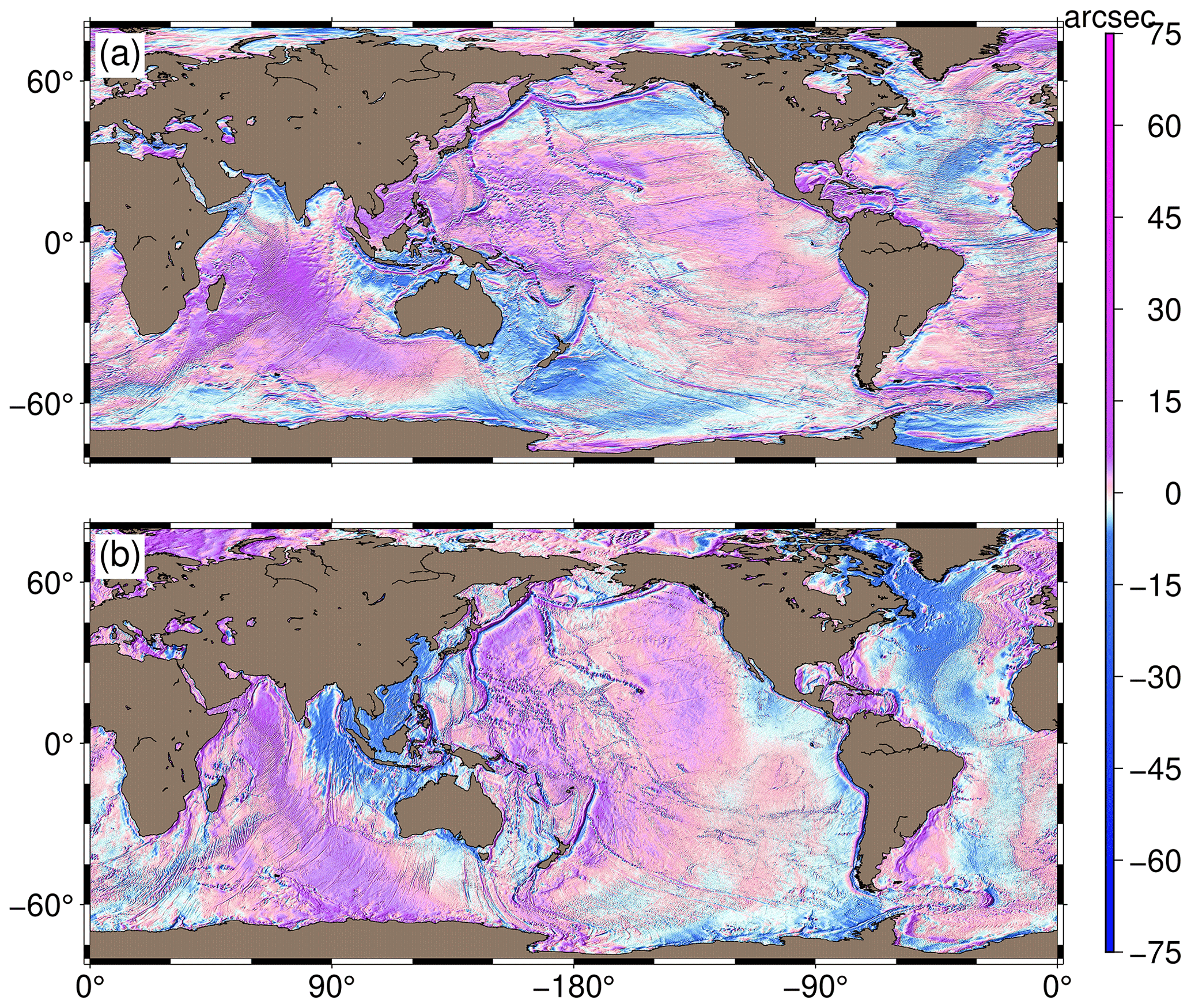
Figure 2 Altimetry-derived deflections of the vertical: (a) north and (b) east components.

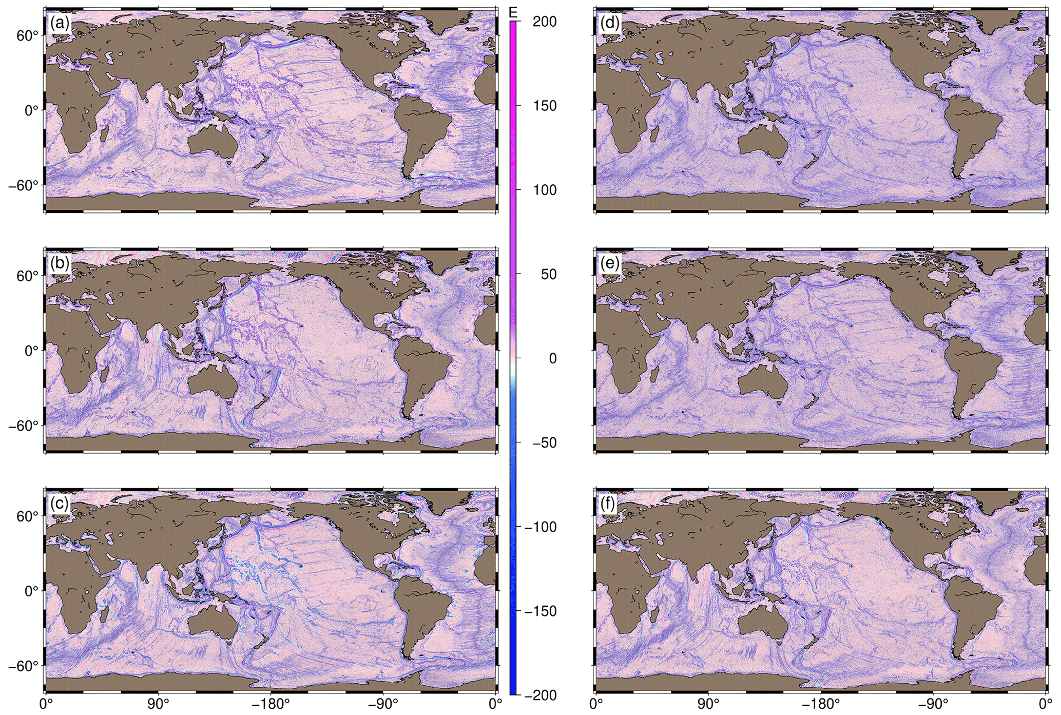
Figure 3 Altimetry-derived gravity gradient tensor: (a) T_xx, (b) T_yy, (c) T_zz, (d) T_xy, (e) T_xz and (f) T_yz.

4 Results and analysis

4.1 Altimetry-derived gravity gradient tensor

The input deflections of the vertical, and the inverted gravity gradient tensor are presented in Figs. 2 and 3, respectively. Gravity gradients are known to be sensitive to topographic variations and, as such, they are good at revealing short-wavelength bathymetric and tectonic features. Even though some tectonic features can be seen in the deflections of the vertical (Fig. 2), they are better depicted in the various components of the gravity gradient tensor. For instance, the outline of the Mid-Atlantic Ridge is well revealed in Fig. 2, whereas its spreading is perfectly exposed in addition to its outline in Fig. 3. Furthermore, the boundaries of the African and South American tectonic plates can be more clearly seen in Fig. 3 than in Fig. 2. Again, the western boundary of the Nazca tectonic plate (which borders the Juan Fernández and Easter microplates in the eastern Pacific Ocean) can be seen in the east deflection component; however, it is better exposed in T_yy, T_zz and T_yz. These observations are attestations to one key characteristic of the gravity potential field: higher differentiations reveal high frequencies.

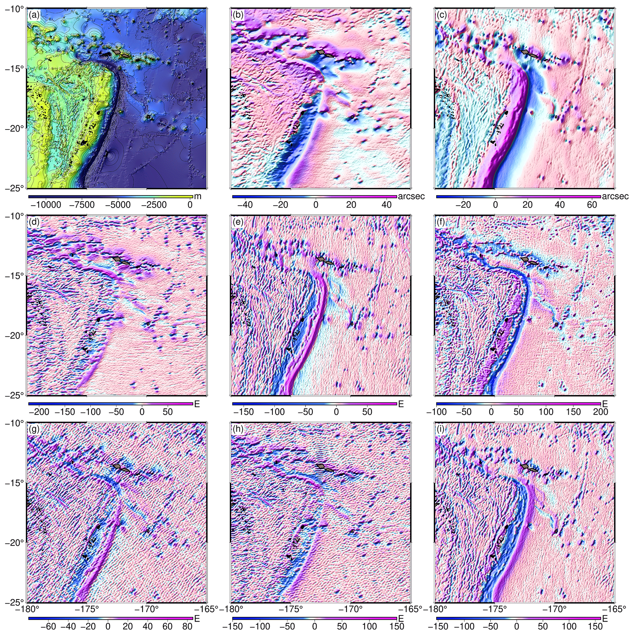
Figure 4 Topography and inverted gravity field signals of the Tonga Trench: (a) multibeam bathymetry, (b) ξ, (c) η, (d) T_xx, (e) T_yy, (f) T_zz, (g) T_xy, (h) T_xz and (i) T_yz.

In order to further substantiate the short-wavelength nature of gravity gradients, Fig. 4 presents the multibeam bathymetry over the Tonga Trench near Fiji in juxtaposition with the inverted gravity field signals. The multibeam depth data were obtained through the AutoGrid web tool of the National Centers for Environmental Information (NCEI: https://www.ncei.noaa.gov/maps/autogrid/, last access: 5 December 2023). From Fig. 4, one can observe bathymetric signatures in the various gravity field signals, including the two components of deflections of the vertical. It is obvious that the bathymetric signatures resolved by the deflections of the vertical have longer wavelengths than those resolved by the gravity gradients. Additionally, this clearly proves that deflections of the vertical also contain valuable bathymetric information that is worth exploiting in the absence of the widely used gravity anomaly and vertical gravity gradient (VGG) (Annan and Wan, 2022).

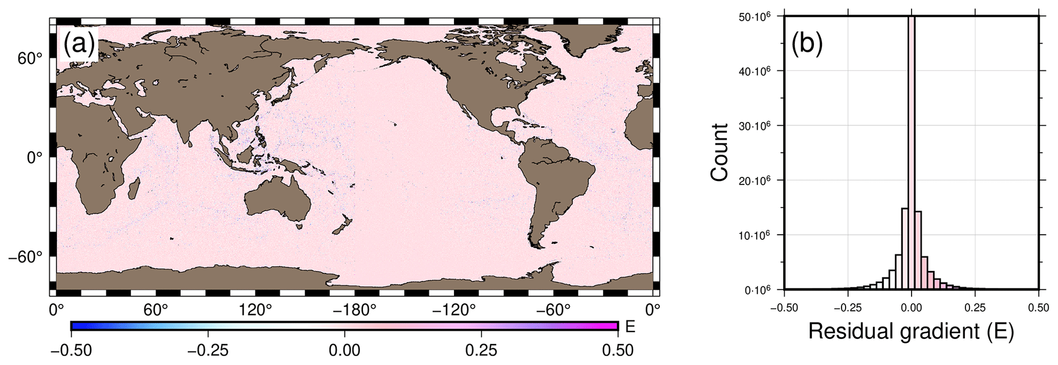
Figure 5 Result of the Laplacian operation: (a) map view and (b) histogram of residual gradient signal.

To check the accuracy of the gravity gradient tensor, we test the Laplacian equation on the gravity gradient tensor, i.e., $T_{xx}+T_{yy}+T_{zz}=\mathrm{0}$. Apart from its ability to tell how accurate the inverted gradient tensor is, the result from the Laplacian equation is also an indication of the effectiveness of the inversion method used to derive the signals. The residual gradient signal shown in Fig. 5 is the result of the Laplacian operation. It can be seen that the residuals are practically zero everywhere. The average residual gradient is −0.0012 E, with a standard deviation of 0.0472 E. The high accuracy reported in Fig. 5 is an alternative interpretation of the accuracy of the altimetry observations. Also, it consequently serves as an indicator of the accuracy of the deflections of the vertical. This is because each component of the gravity gradient tensor is computed from the same north–south and east–west components of the deflections of the vertical.

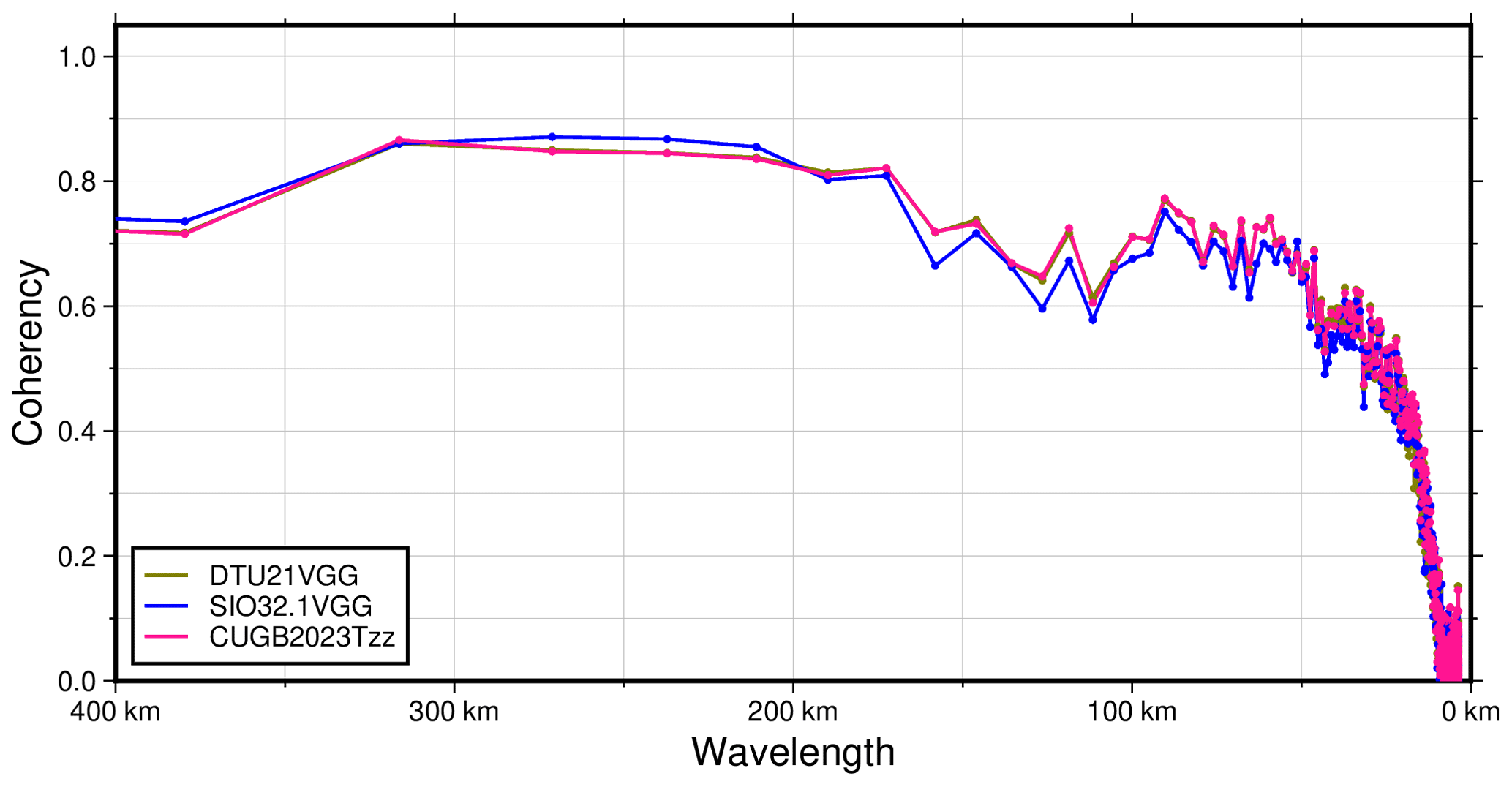
Figure 6 Coherency between vertical gravity gradient and multibeam bathymetry of the Tonga Trench.

Additionally, the coherency between the inverted T_zz and multibeam bathymetry of the Tonga Trench was computed. The result is juxtaposed with corresponding coherency values computed from the DTU21GRA-derived T_zz and SIO's VGG product (i.e., curv_32.1.nc) as shown in Fig. 6. The curves in Fig. 6 are nearly identical, with low coherency values seen at low wavelengths. The small coherency values at the low wavelengths are caused by upward continuation of gravity field from the seafloor to the sea surface (Smith and Sandwell, 1994). Analysis of Fig. 6 shows that with a minimum coherency of 0.5, the inverted T_zz and the VGGs from DTU and SIO would poorly detect bathymetric features with wavelengths less than 25 km. Bathymetric features with wavelengths greater than 45 km would be detected with higher accuracy. This is because the coherency values of these wavelengths are greater than or approximately equal to 0.60 in each of the three vertical gravity gradients. It can be seen that the inverted T_zz is slightly closer to the signals from DTU than those from SIO.

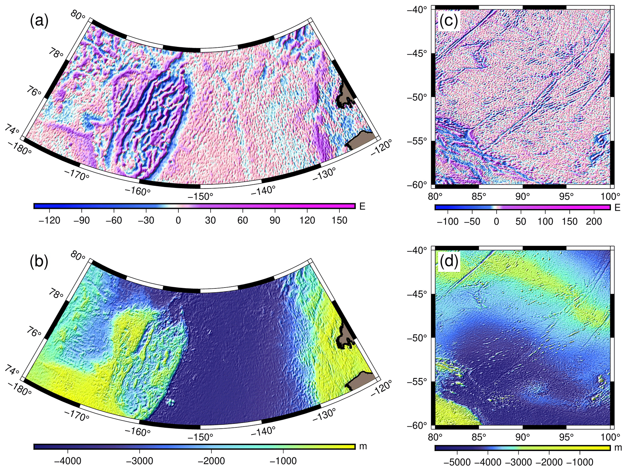
Figure 7 (a) Vertical gravity gradient and (b) predicted bathymetry of Arctic Ocean region; (c) vertical gravity gradient and (d) predicted bathymetry of south Indian Ocean region.

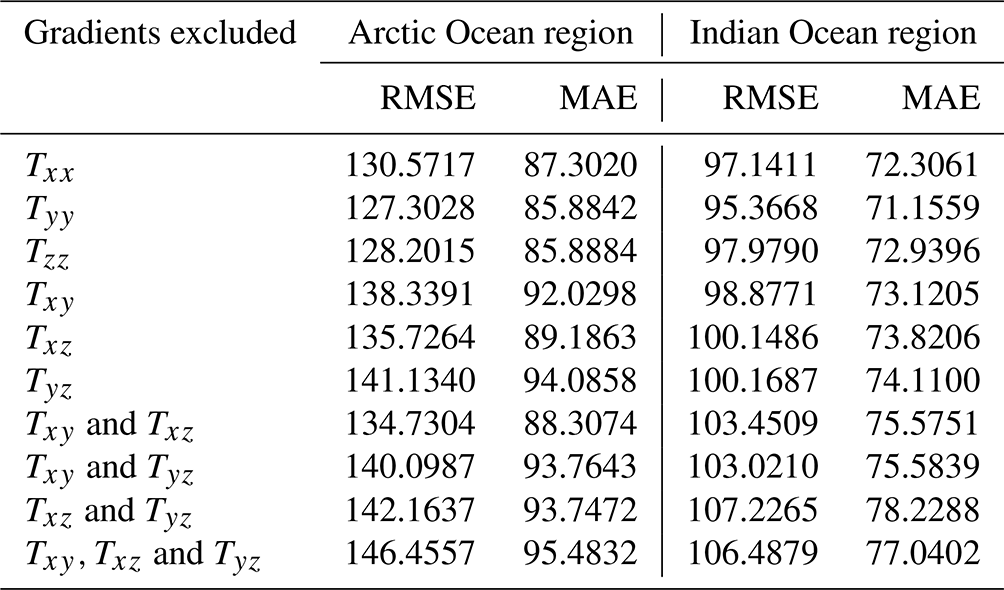
Table 1 Analyzing the bathymetric influence of the gravity gradients (unit: m).

4.2 What is the utility of having all six gravity gradients?

To answer this question, we adapted the deep learning method of bathymetry inversion developed by the authors in Annan and Wan (2022) to assess the bathymetric significance of each tensor component. We assume that the most accurate bathymetric model would be obtained from the combined use of all six gravity gradients. Therefore, bathymetry inversion was performed with systematic omission of each gravity gradient with replacement. For each bathymetric model, the root mean squared error (RMSE) and mean absolute error (MAE) relative to shipboard depths at test points were computed. It implies that the largest RMSE and MAE will correspond to the most influential gravity gradient. This analysis was conducted in local regions in the Arctic (180–120° W, 74–80° N) and south Indian (80–100° E, 60–40° S) oceans. The predicted bathymetries are juxtaposed with their respective T_zz in Fig. 7. The depth datasets used for training the deep learning model are single-beam soundings provided by NCEI (https://www.ncei.noaa.gov/maps/trackline-geophysics/, last access: 3 December 2023). Table 1 gives a summary of the bathymetric influence of the gravity gradients. In the Arctic Ocean region, the three most influential gravity gradients ranked in increasing order are T_xz, T_xy and T_yz, whereas in the south Indian Ocean region, the order was T_xy, T_xz and T_yz. It is worth mentioning that T_xz and T_yz possess information in both vertical and horizontal directions; thus, it is possible that in addition to the vertical information, the horizontal information in these two gradients also contribute to refining bathymetric prediction.

Indeed, there are previous works that have inverted bathymetry from T_zz (Hu et al., 2021, 2014, 2015; Tozer et al., 2019); however, as shown in this section, T_zz is not the most dominant gravity gradient for bathymetric prediction. The results from this analysis are consistent with findings in our previous study (Wan et al., 2023), in which a shallow neural network was adapted for bathymetric predictions.

Apart from bathymetry inversion, gravity gradients can also be used for identifying seamounts (Kim and Wessel, 2015) and for studying their evolution (Wessel et al., 2022). Another interesting application of gravity gradients was conducted by Harper et al. (2021), in which seafloor spreading was studied by analyzing the distribution and tectonic importance of “see-saw” ridges. It is worth mentioning that the findings of Kim and Wessel (2015), Wessel et al. (2022) and Harper et al. (2021) were all derived from T_zz only, which is in the vertical direction only. Therefore, by having access to the full gravity gradient tensor from the present study, in addition to the vertical perspective from T_zz, it would be more interesting to analyze their findings from different directions if the other five tensor components are used.

In summary, the gravity gradients presented in this paper prove that the high spatial density and SSH accuracy of currently available GM datasets are capable of resolving the various components of Earth's gravity gradient tensor over the oceans. The results from this study further substantiate a statement of Sandwell et al. (2013), who recently asserted that gravity field signals inverted from current generation of altimetry datasets are becoming more superior in quality than most of the publicly available shipborne gravimetry datasets. Therefore, if the geoscience community would invest similar efforts in the techniques of inverting full tensor of gravity gradients like has been invested in gravity anomaly and VGG, the accuracy of future models of gravity gradient tensors would improve. We say this in light of the high range accuracy of the Ka-band mission (i.e., SARAL/AltiKa), as well as the high across-track sampling from Cryosat-2 and the recently launched SWOT mission, which incorporates interferometric technology.

5 Data availability

The global marine gravity gradient tensor model CUGB2023GRAD is available at the ZENODO repository: https://doi.org/10.5281/zenodo.10511125 (Annan et al., 2024). The dataset consists of GMT-readable geospatial grids in NetCDF file format (i.e., vector of latitudes, vector of longitudes and matrix of gravity gradients).

6 Conclusion

Components of deflections of the vertical, inverted from altimetry-derived SSHs, have been used as input signals to invert marine gravity gradient tensor over the globe. The resultant gravity gradient tensor was assessed via the Laplacian equation, with the corresponding residual gradient having magnitudes close to zero across the globe. Assessment of the inverted T_zz through bathymetric coherence analysis showed that it correlates well with multibeam depths. Further analysis at local regions in the Arctic and south Indian oceans proved that the frequently used vertical gravity gradient is not the most dominant tensor component for bathymetric prediction. Instead, the most influential tensor components are the three non-diagonal gravity gradients, thereby proving that the bathymetric and tectonic information in the other five gravity gradients are worth exploiting. The average across-track sampling of current generation of altimetry observations is better than the 8 km minimum required for gravity field inversion. Therefore, with the anticipated higher accuracy and better spatial resolution of the recently launched SWOT mission and upcoming Ka-band altimetry missions, coupled with an increase in research interest and investment, the accuracy of future gravity gradient tensor models should improve.