the Creative Commons Attribution 4.0 License.
the Creative Commons Attribution 4.0 License.
 | 01 Mar 2024
A global dataset of the shape of drainage systems
Ci-Jian Yang
Jens M. Turowski
Richard F. Ott
Jean Braun
Hui Tang
Shadi Ghantous
Xiaoping Yuan
Gaia Stucky de Quay
Drainage basins delineate Earth's land surface into individual water collection units. Basin shape and river sinuosity determine water and sediment dynamics, affecting landscape evolution and connectivity between ecosystems and freshwater species. However, a high-resolution global dataset for the boundaries and geometry of basins is still missing. Using a 90 m resolution digital elevation model, we measured the areas, lengths, widths, aspect ratios, slopes, and elevations of basins over 50 km2 globally. Additionally, we calculated the lengths and sinuosities of the longest river channels within these 0.67 million basins. We built a new global dataset, Basin90m, to present the basins and rivers, as well as their morphological metrics. To highlight the use cases of Basin90m, we explored the correlations among morphological metrics, such as Hack's law. By comparing with HydroSHEDS, HydroATLAS, and Google Earth images, we demonstrated the high accuracy of Basin90m. Basin90m, available in shapefile format, can be used on various GIS platforms, including QGIS, ArcGIS, and GeoPandas. Basin90m has substantial application prospects in geomorphology, hydrology, and ecology. Basin90m is available at https://doi.org/10.5880/GFZ.4.6.2023.004 (He et al., 2023).
- Article
(11455 KB) - Full-text XML
- BibTeX
- EndNote


Drainage divides and rivers are among the most recognizable features on Earth's surface. The shape of drainage basins and rivers has significant implications for landscape evolution processes and dynamics (Kirchner et al., 2001; Shelef, 2018; Ielpi et al., 2023; He et al., 2024). With equal basin lengths, a broader basin collects more precipitation, thus offering a more stable discharge and water level, reducing the risk of rivers drying up. A stable water level benefits ecological integrity, water use, and navigation (Datry et al., 2023). Broader basins typically have longer and more intricate river networks, affecting flood risk associated with both extreme rainfall and glacial lake outburst events. In broader basins, rainwater takes more time to reach the main stream, indicating a longer arrival time of flood peaks. A glacial lake outburst flood travels a longer path in a broader basin, losing more energy and surface runoff. Hence, communities downstream of a broader high-mountain catchment encounter less threat from a single glacial lake outburst flooding. However, as broader basins have more tributaries with risks of glacial lake outbursts, timely and accurate early flood warnings require the deployment of more seismic stations within the basin (Maurer et al., 2020; Cook et al., 2021).
Furthermore, broader basins can contain a greater variety of tributaries and habitat types. This heterogeneity of habitats allows these basins to host a greater diversity of species, especially aquatic, amphibious, and riparian organisms, by providing more ecological niches across the landscape (Matthews and Robison, 1998). Similarly, meandering rivers create a mosaic of habitats with varying flow velocities, depths, and substrates, supporting the diversity of aquatic organisms (Nagayama and Nakamura, 2017; Rhoads et al., 2003; Yu et al., 2022).
Meanwhile, given the same elevation drop, a meandering river has a milder channel gradient than a straight river and therefore features lower erosion rates. Additionally, the shape of drainage systems has been argued to be related to climatic and tectonic conditions (Castelltort et al., 2012; Ielpi et al., 2023; Luo et al., 2023; Sreedevi et al., 2009; Strong and Mudd, 2022) and could therefore be used as an archive to reconstruct Earth's history. Accordingly, a global dataset on the shape of drainage systems benefits scientists and policymakers in geomorphology, hydrology, and ecology, fostering interdisciplinary collaborations.
Since the 21st century, digital elevation models (DEMs) have been utilized to produce several global-scale drainage basin and river databases (Allen and Pavelsky, 2018; Amatulli et al., 2022; Lin et al., 2021; Masutomi et al., 2009; Shen et al., 2017; Vörösmarty et al., 2000). Using a 1 km resolution DEM, the US Geological Survey (USGS) developed HYDRO1k (USGS, 2000), a global hydrological dataset providing vector basin boundaries and river channels. HydroSHEDS (Lehner and Grill, 2013; Lehner et al., 2008) provides 500 m resolution global basins and rivers and their basic metrics, such as area, river length, and stream order. HydroSHEDS basin boundaries and a 500 m resolution DEM were utilized to calculate morphometric indices for 26 272 drainage basins worldwide with an area larger than 100 km2 (Guth, 2011). These indices include basin elevation and slope. HydroATLAS was also developed based on HydroSHEDS and incorporates 56 hydro-environmental attributes, including basin mean slope and elevation (Linke et al., 2019).
The above datasets lack measurements of drainage basin length and aspect ratio. Shen et al. (2017) used a 1 km DEM to obtain the global distribution of basin length and elongation ratio. However, the dataset is in raster format, without vectorial basin boundaries and rivers. More importantly, the spatial resolutions of all the above databases are relatively low. With the advancements in computer performance and algorithms, the 90 m resolution DEMs are being used to establish global databases of drainage systems. For example, the HDMA released by USGS includes nearly 295 000 drainage basins but only contains information on drainage areas (Verdin, 2017). GRNWRZ comprises a global river database at a resolution of 90 m that includes information on river lengths (Yan et al., 2022). This database offers the boundaries and areas of water resource zones, which are distinct from drainage basins.
In summary, catalogs of drainage basins and rivers are available, along with measurements of the area, slope, and elevation of basins. Yet, many datasets were based on DEMs with resolutions of 500 m or coarser, and few works have focused on more complex basin characteristics, such as aspect ratio, which describes the shape of drainage basins, and sinuosity, which characterizes the shape of river channels. Furthermore, some databases only offer raster formats without vector accessibility. Moreover, the download links of some datasets are invalid (e.g., Vörösmarty et al., 2000; Guth, 2011).
Here, we provide an updated global catalog of drainage systems, making all relevant files and the script available and including a wide range of geometric characteristics. We used a global 90 m resolution DEM and obtained over 665 000 drainage basins with a size over 50 km2. For each basin, we extracted the longest river channel that extends from the drainage divide to the river mouth. Additionally, we measured parameters for each drainage system, including stream order; the length, width, aspect ratio, slope, and elevation of basins; and the length and sinuosity of rivers. The spatial distribution of drainage systems and their morphological parameters constitute a drainage system shape dataset, Basin90m.
We divided the global DEM into 130 segments to accommodate the computational capabilities (Figs. 1 and 2a). We selected a basin in Madagascar to demonstrate the steps of obtaining drainage basins and their longest rivers from a DEM. First, we calculated flow direction and accumulation for each point within the basin. Based on flow direction and accumulation, we delineated basins and rivers of different stream orders (Fig. 2b). Once the spatial distribution of basins and rivers was obtained, we measured parameters describing the size and shape of the drainage systems (Fig. 2c). Finally, basins with over half of their area located in lakes or sandy deserts were removed (Fig. 2d).
Conventional GIS platforms such as QGIS and ArcGIS provide various hydrology tools, such as extracting drainage basins and river channels. However, we need to process 130 DEMs and calculate some metrics, such as basin width, for which no tools are readily available within these GIS platforms. Therefore, we used the TopoToolbox software (Schwanghart and Scherler, 2014) to automate the extraction of drainage systems and the calculation of various metrics in a single script. TopoToolbox is a MATLAB toolbox for analyzing and manipulating geospatial data, supporting drainage basin delineation and topographic-property calculation. In addition to utilizing the functions in TopoToolbox, we developed new algorithms to measure basin length and width. We integrated all these functions into an automated workflow that delineates drainage basins and channels across all stream orders and measures their morphological attributes.
All the operations described below in Sect. 2.2 to 2.6 were automated within our TopoToolbox script. The script inputs a single DEM and outputs vector files (Esri shapefiles) for basins and rivers. Refer to the “Code availability” section for the download link of this script. Shapefile is a data format that stores geographic vector data, including geometry and attributes. Parameters describing the morphology of drainage systems were stored in the attribute table of basin shapefiles. The computation of all 130 DEMs was carried out on the high-performance computing platform of the German Research Centre for Geosciences.
2.1 DEM preprocessing
The 90 m resolution Shuttle Radar Topography Mission (SRTM) DEM is a widely used dataset for global geomorphological analyses (Farr et al., 2007). It covers the Earth's land surface between 60° N and 56° S in latitude. Due to limitations in computer memory, it is a common practice to partition global DEMs into smaller segments (Amatulli et al., 2022). To ensure the integrity of each drainage basin and river channel, we partitioned the global DEM based on drainage divides provided by HydroBASINS (Lehner and Grill, 2013). We used the Clip Tool in ArcGIS (version 10.2) to cut the global DEM into 130 segments (Figs. 1 and 2a). By utilizing drainage divides corresponding to the largest basins in a region, we ensure that continents are cropped in a way that avoids splitting any basins internally. Many islands were treated as a single DEM segment, such as New Zealand (Fig. 1).
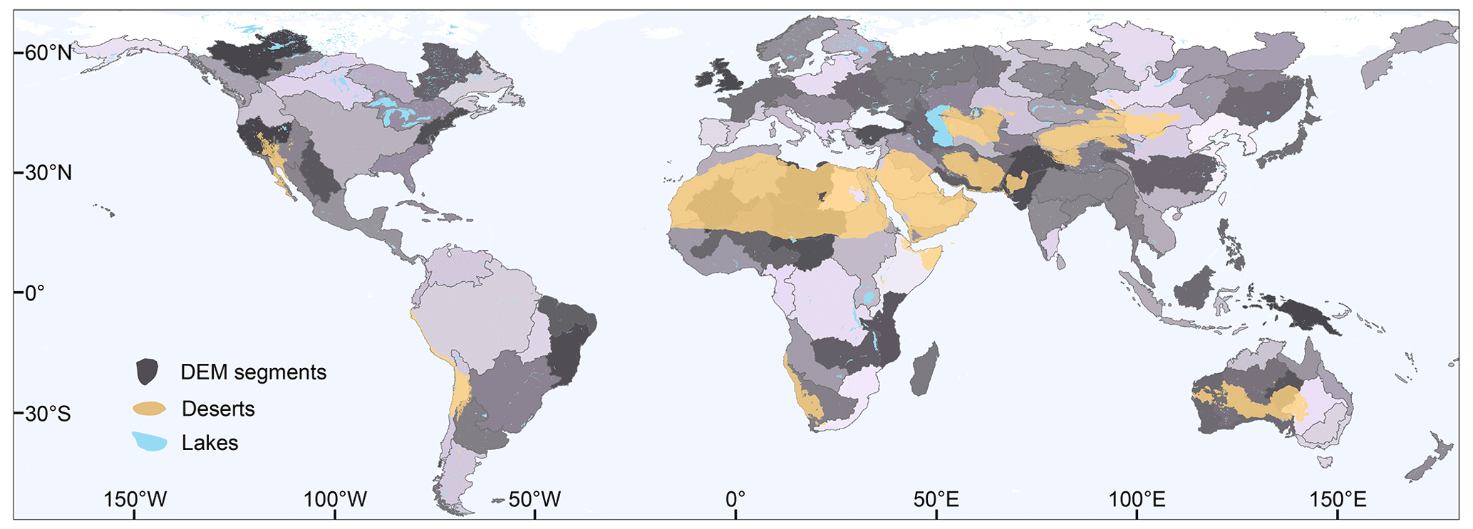
Figure 1DEM segments (N=130) based on the drainage divides from HydroBASINS (Lehner and Grill, 2013). Different shades of gray were used to distinguish different DEM segments. Lakes were obtained from HydroLAKES (Messager et al., 2016). We consider regions with an aridity index less than 0.08 to be sandy deserts (see Sect. 2.7 for details).
2.2 Flow direction
The first step toward obtaining drainage basins and river networks from a DEM is calculating flow direction and accumulation. Flow direction describes the drainage direction of each cell. Flow networks derived from DEMs are affected by measurement and data-processing errors (Schwanghart et al., 2013). DEM elevations in valley bottoms can be overestimated due to steep hillslopes, water, and vegetation (Schwanghart and Scherler, 2017). Therefore, we used the carving method to generate flow directions to ensure channels are well connected despite local noise (Lindsay, 2016; Schwanghart et al., 2013; Schwanghart and Scherler, 2017).
Once carving is complete, we used the D8 method to determine flow direction (Tarboton, 1997). This method assumes that water flows downslope from each cell to one of its eight neighboring cells (Fig. 2b). A single flow direction out of the eight possible directions is assigned to each cell of the DEM (Fig. 2b) by comparing the elevations of neighboring cells and identifying the steepest descent path. We adopt integers from 1 to 8 to differentiate the possible directions. If a cell has a flow direction of 5, it indicates that all water passing through that cell will be directed toward its left neighbor (Fig. 2b).
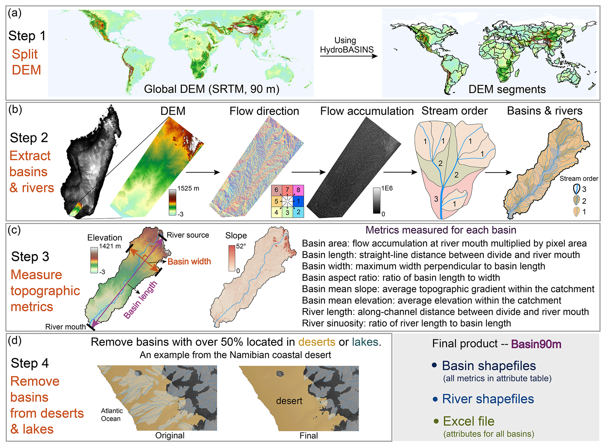
Figure 2Flowchart illustrating the processes of extracting global drainage systems and their morphological metrics. (a) The global DEM was partitioned into 130 segments using drainage divides provided by HydroBASINS (Lehner and Grill, 2013). (b) Menarandra River basin in southern Madagascar was chosen as an example to demonstrate the steps of extracting drainage basins and the longest river channels with various stream orders. (c) Based on the spatial distribution of basins and river channels, eight parameters describing the drainage system's size and morphology were automatically measured using a MATLAB script. (d) Drainage basins that have over half of their area within lakes or sandy deserts were removed.
2.3 Flow accumulation
Flow direction is the basis for calculating flow accumulation, a measure that quantifies the cumulative number of cells contributing to a given point (Fig. 2b). Flow accumulation starts from zero at the basin boundary, increases downstream, and reaches a maximum at the river mouth. River mouths can be river confluences, lakes, or seas. Therefore, basin area can be obtained by multiplying flow accumulation at the river mouth by the area of one pixel. With flow direction and accumulation, we can delineate stream orders and extract basins and rivers.
2.4 Stream order
Large drainage basins contain small catchments. We assigned Strahler stream orders to basins and their longest rivers for hierarchical classification to capture the topological relationship between catchments. Strahler stream order quantifies the hierarchy of basins and river segments within a river network (Strahler, 1957). It assigns an integer to each segment based on the contributing tributaries (Fig. 2b). First-order rivers are found near basin boundaries. Stream order increases downstream. When two segments of the same order converge, they merge to form a new segment with an order increase of 1. If two segments of different orders merge, the resulting segment inherits the higher order. For example, a first-order segment merging with a second-order segment results in a second-order segment.
The magnitude of stream order within a drainage basin depends on the area threshold of the first-order basin. The larger the threshold, the fewer orders in the entire catchment. Limited by computing resources, we only extracted drainage basins with an area ≥50 km2. An area of 50 km2 contains about 6000 cells, sufficient to organize a drainage system. Basins with areas less than 50 km2 were not extracted, thus not contributing to the stream order of downstream basins. However, those small basins contribute to water discharge of their downstream channels.
2.5 Drainage basins and the longest rivers
We extracted only the longest river of each basin (Fig. 2b). In nature, rivers commonly develop a certain distance downstream of drainage divides; this distance is known as hillslope length. For example, the average hillslope lengths in Taiwan and Sicily are 1556 and 1756 m, respectively (He et al., 2021a). A common approach is to designate the point where the upstream area exceeds a channelization threshold as the river source. For instance, the two latest global river databases, MERIT Hydro (Lin et al., 2021) and Hydrography90m (Amatulli et al., 2022), employ channelization thresholds of 1 and 0.05 km2, respectively. Since Basin90m utilizes the straight-line distance between the river source and mouth as the basin length, we selected a channelization threshold of zero, indicating that rivers originate from drainage divides.
We use Menarandra River basin in Madagascar as an example to illustrate the steps for obtaining drainage systems (Fig. 2b, c). This basin consists of three stream orders, including 1 order-3, 10 order-2, and 46 order-1 sub-basins. The third-order basin has an area of 8701 km2 and a basin aspect ratio of 3.3. The corresponding river length and sinuosity are 295 km and 1.6, respectively.
2.6 Morphological indices
We measured the basic geometric parameters after obtaining basin boundaries and the longest rivers. For basins, the parameters include area, length, width, aspect ratio, and average slope and elevation (Fig. 2c). For rivers, we measured along-channel length and sinuosity (Fig. 2c). All parameters were automatically computed with our TopoToolbox script. For instance, the straight-line distance between the river source (drainage divide) and mouth of the longest channel is termed basin length. Basin width is defined as the greatest distance measured along a straight line perpendicular to the direction of the basin length at the two points where the line intersects the basin boundary. The sum of the elevations of all pixels within a basin divided by the number of pixels yields the basin mean elevation. We report all metrics and stream order values for catchments over 50 km2. The value of these metrics is stored in the attribute table of each basin shapefile data item. See the “Data availability” section for details.
2.7 Removing basins from lakes and deserts
After obtaining the global distribution of drainage systems, we removed basins and rivers associated with lakes and sandy deserts (Fig. 2d). Basin90m aims to provide drainage systems created by surface water flow processes. While lakes are related to water flow, it is inappropriate to consider a drainage basin completely within a lake. We need a global lake database to remove drainage systems within lakes. Several global lake datasets are available, such as HydroLAKES (Messager et al., 2016), GloLakes (Hou et al., 2024) and Lake-TopoCat (Sikder et al., 2023). Here, we used HydroLAKES, which includes 1.4 million lakes worldwide, with an area range of 0.1–377 002 km2. Since the minimum basin area in Basin90m is 50 km2, we only retained 3402 lakes with a size over 50 km2 (Fig. 1).
Due to high permeability and intense evaporation, sandy deserts are typically unable to sustain surface water. Therefore, basins and rivers derived from DEMs within sandy deserts are unlikely to accurately reflect river dynamics. To our knowledge, no published global dataset for sandy deserts exists. As a result, we relied on using aridity index to determine the location of such regions. Aridity index is a measure that quantifies the dryness or aridity of a region based on the ratio of precipitation to potential evapotranspiration. A lower aridity index indicates a drier environment. Therefore, aridity index is closely associated with desert formation (Gamo et al., 2013).
Here, we used the Global-AI_PET_v3 (Zomer et al., 2022), a global aridity index dataset, to delineate sandy deserts. By comparing the regions obtained using multiple aridity index thresholds with the distribution of sandy deserts on Google Earth, we classified areas with aridity index values of less than 0.08 as sandy deserts. This threshold captures the majority of sandy deserts while avoiding misclassifying excessive non-desert regions.
Using the Python-based GeoPandas library, we removed basins with over half of their area within lakes or sandy deserts (Fig. 2d). We also removed the river channels within those deleted basins. In addition, we manually removed all drainage systems intersecting with the 60° N latitude line in ArcGIS to avoid incomplete river networks due to DEM coverage. In the end, out of the 840 000 basins obtained in Sect. 2.5, approximately 170 000 were removed, retaining 667 629 basins and their longest rivers.
Through the steps above, we obtained the spatial distribution of global drainage systems and their morphological metrics. Next, we analyze the distribution and correlations of these metrics in Basin90m. First, we present the differences in drainage systems with different stream orders. Then, we show the distribution of metrics that describe the morphology of drainage systems. Afterward, we present the interrelationships among these metrics. For example, utilizing Basin90m, we derived Hack's law (Hack, 1957) fitted from global data.
3.1 Basins with different stream orders
Figure 3a shows basins in Basin90m with stream orders ranging from 4 to 9. Three ninth-order basins are the Amazon, Nile, and Congo, with areas of 6 038 417, 2 895 947, and 3 716 644 km2, respectively. Eighth-order basins are widely distributed globally, including the Mississippi in North America, the Río de la Plata in South America, the Orange in Africa, the Yangtze and Mekong in Asia, and the Murray–Darling in Australia. Basins with the highest stream order in a region often occupy a significant portion of the area. For example, Madagascar has a basin with a stream order of 6, covering an area of 59 200 km2, approximately 10 % of Madagascar's total area. Taiwan island has two basins with a stream order of 4, each with an area of about 30 000 km2, together occupying one-sixth of the island.
Figure 3b–g illustrates the statistics of drainage systems with different stream orders. As stream order increases, the number of basins and total river length exponentially decrease (Fig. 3b, c). The number of first-order basins is 521 857, accounting for 78 % of the total basin count. There are 661 397 basins with orders 1–3, representing 99 % of the total basin count. In contrast, only 90 basins are of the highest stream orders (7–9). The total basin area is determined by multiplying the basin count with the average basin area. As stream order increases, the average basin area increases, while the basin count decreases. Therefore, total basin area does not monotonically change with stream order (Fig. 3d). The average basin area and river length increase with increasing stream order because higher-order basins encompass lower-order basins (Fig. 3e, f).
River sinuosity generally increases with stream order (Fig. 3g) as higher-order basins provide more space for rivers to meander (Biron et al., 2014). The lack of significant changes in basin aspect ratio with increasing stream order (Fig. 3h), along with the absence of a correlation between basin topography (slope and elevation) and stream order (Fig. 3i, g), supports the concept of self-similarity in drainage basins (Bennett and Liu, 2016; Mantilla et al., 2010; Sassolas-Serrayet et al., 2018).
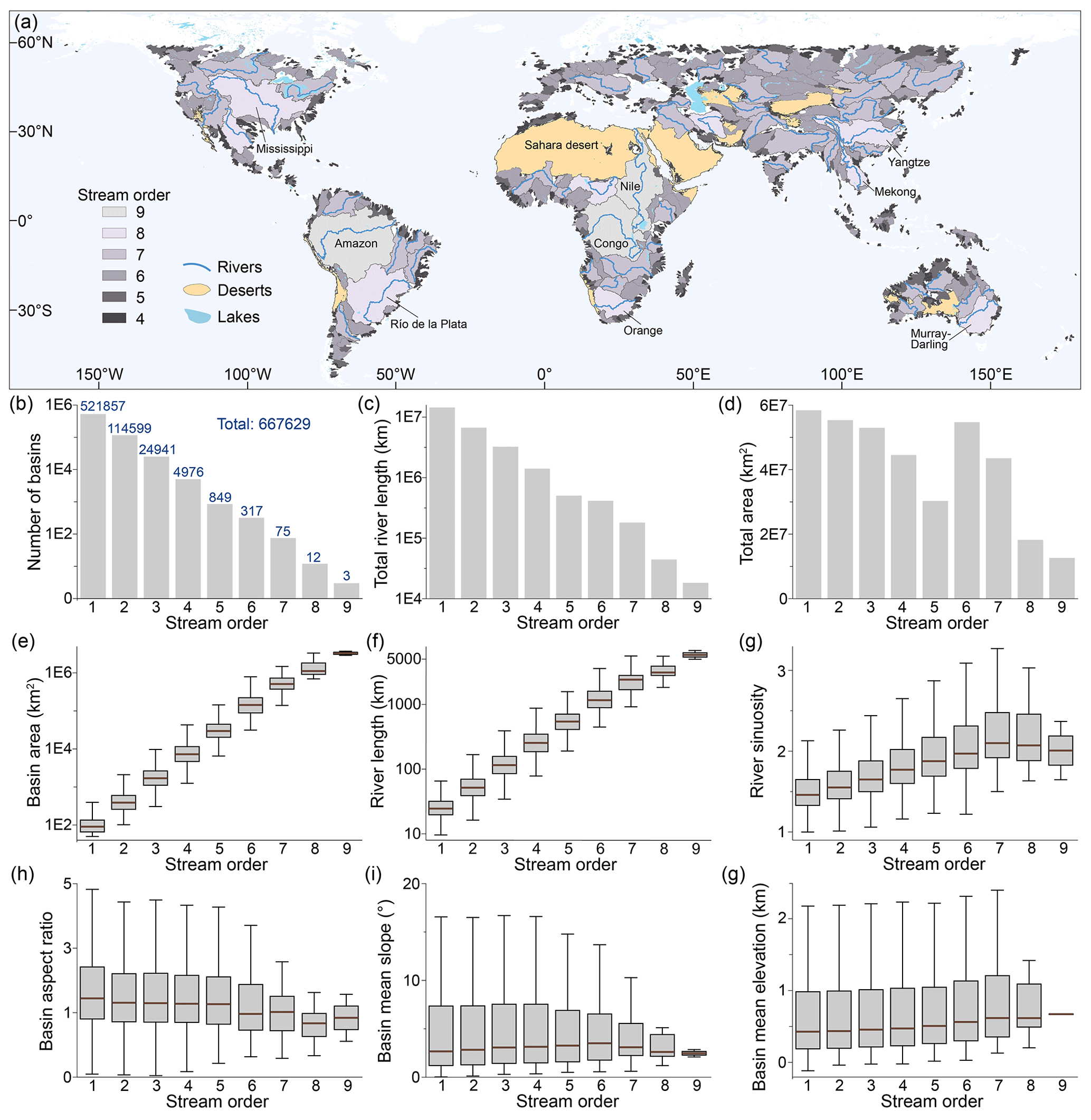
Figure 3Global drainage systems with nine stream orders. (a) The spatial distribution of basins with orders from 4 to 9. Rivers with stream orders from 7 to 9 are displaced. (b–g) Morphological metrics displayed by stream orders.
3.2 Distribution of morphological metrics
We present the probability densities and spatial patterns of metrics that describe the morphology of drainage systems. Most morphological metrics have left-skewed, log-normal distributions (Fig. 4). A total of 95 % of basins have an area smaller than 1000 km2. There are only 2868 basins with a size larger than 10 000 km2 (Fig. 4a). Most (88 %) basins have a length ranging from 10 to 50 km, with an average value of 25 km (Fig. 4b). The number of basins with lengths exceeding 100 km is 11 357, accounting for only 1.7 %. The average basin length is roughly twice the basin width.
Many basins (N=89 673) have an average width ranging from 5 to 25 km, constituting 87 % of the total (Fig. 4c). The number of basins with an aspect ratio between 1 and 5 is 598 426, accounting for 90 % of all basins (Fig. 4d). A basin aspect ratio less than 1 typically indicates a deviation between the overall flow direction and basin elongation direction. This scenario is observed in only 5 % of the basins (N=34 357), suggesting a rare deviation between basin elongation and overall water flow.
The average slope shows a wider distribution compared to the other parameters. It is distributed between 0 and 40°, with an average value of 5.4° (Fig. 4e). The distribution of basin mean elevation has multiple peaks (Fig. 4f). Among them, the peak at an elevation of 4500 m corresponds to the Tibetan Plateau and Andes. Over 95 % of the river lengths are smaller than 100 km (Fig. 4g). The number of basins with river lengths exceeding 100 and 1000 km is 31 392 and 370, respectively. Since river sinuosity is the ratio between the along-channel and straight-line distance from the drainage divide to the river mouth, the minimum sinuosity is 1. Basins with a river sinuosity of less than 2 account for 91 %, with an average value of 1.6 (Fig. 4h).
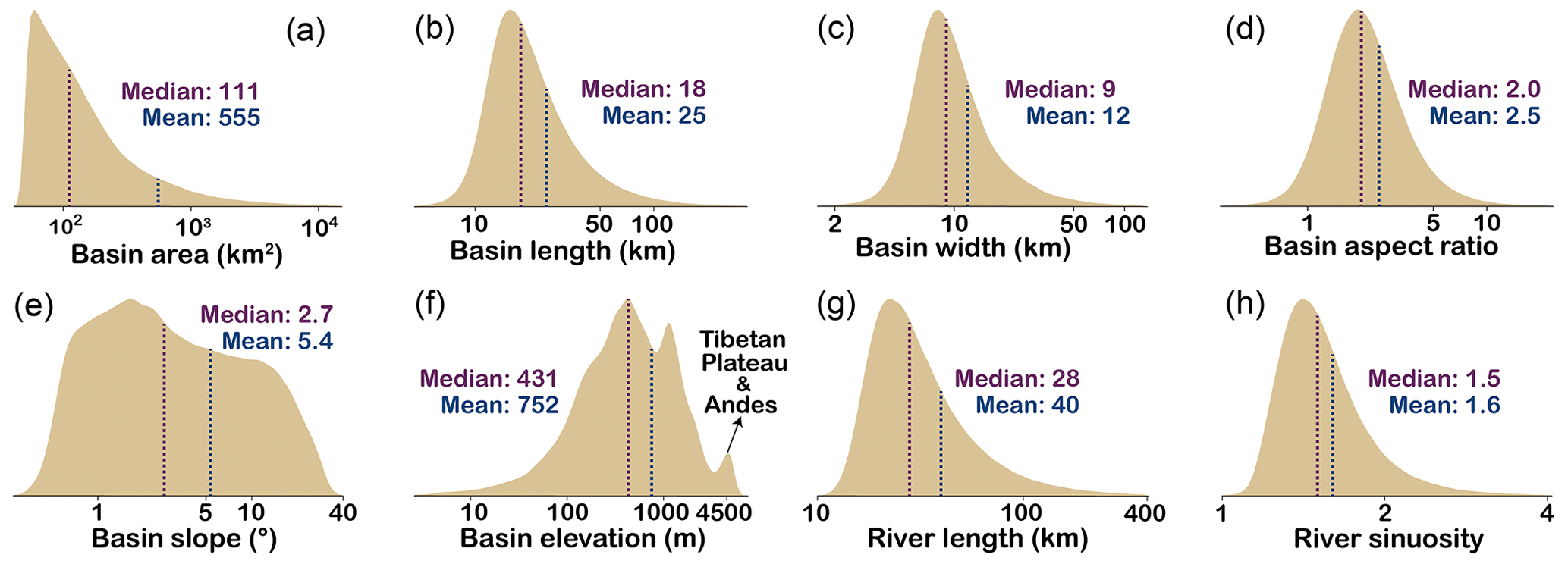
Figure 4The probability density estimation shows the distribution of morphological metrics. All basins in Basin90m were used for probability density estimation without distinguishing stream orders. The x axis of all subfigures is logarithmically scaled with a base of 10. (a) Basin area. (b) Basin length. (c) Basin width. (d) Basin aspect ratio. (e) Basin mean topographic slope. (f) Basin mean elevation. (g) River length. (h) River sinuosity. Dashed purple and blue lines indicate the median and the mean, respectively.
Basin90m includes eight metrics for each drainage system (Figs. 2c and 4). Here, we present the spatial distribution of four metrics (Fig. 5). The first parameter is drainage area, describing basin size. There are 12 basins with an area larger than 1×10⁶ km2, with stream orders ranging from 7 to 9 (Fig. 5a). The second parameter is aspect ratio, illustrating basin shape. A higher aspect ratio indicates a more elongated basin. There is no clear relationship between aspect ratio and stream order (Fig. 3h). As a result, the most elongated basins can be large and small (Fig. 5b). Numerous elongated basins characterize the periphery of the Tibetan Plateau. An aspect ratio smaller than 1 indicates that the overall flow direction is not aligned with basin elongation direction. For example, the Congo River flows from east to west, while the elongation direction of the basin is north–south. This results in an aspect ratio of 0.9 for the Congo Basin.
The third metric is the average slope of the basin, demonstrating the topographic variations within the catchment. Due to the significant elevation differences between the Tibetan Plateau and the surrounding plains, steep basins developed around the plateau (Fig. 5c). The average slopes of the Yangtze, Salween, and Red basins around the plateau margin are 13, 17, and 18°, respectively. In contrast, the slopes of the Murray–Darling, Mississippi, and Amazon basins are only 1, 2, and 3°, respectively. The fourth parameter is river sinuosity, describing the shape of the longest river. A high sinuosity indicates a meandering river, while a sinuosity closer to 1 indicates a straight river. The sinuosities of the Nile, Danube, Amazon, and Mississippi rivers are 1.6, 1.8, 2, and 2.3, respectively (Fig. 5d).

Figure 5Global distribution of drainage systems with various metrics. Note that higher-order basins cover the lower-order basins. Drainage basins colored by basin area (a), basin aspect ratio (b), basin mean topographic slope (c), and river sinuosity (d). Rivers with stream orders from 7 to 9 are displaced.
3.3 Relationship between morphological metrics
The eight metrics in Basin90m describe the size and shape of drainage systems from various perspectives. The correlation among these parameters is crucial for understanding landscape dynamics; thus, we present a visualization of their relationships (Fig. 6). Overall, there is a strong correlation among parameters that describe similar features (Fig. 6a). For instance, the correlation coefficient between basin length and river length is 0.97, suggesting that river channels and basins tend to grow or shrink simultaneously. The expansion and contraction of basins are achieved through drainage divide migration, which redistributes the lengths of river channels on both sides of the drainage divide (Habousha et al., 2023; He et al., 2021b). Conversely, parameters describing different features typically exhibit a weak correlation. For example, the correlation coefficient between the area representing basin size and the slope describing topography is approximately zero (Fig. 6a).
Figure 6b displays 2D density plots of correlated parameters. Basin area increases with increasing basin length and width. This result is expected since basins often become wider as they grow in length (correlation coefficient of 0.83, Fig. 6a), and both length and width determine basin area. Another example is the relatively high correlation between elevation and slope, which indicates that basins with steeper slopes tend to develop at higher elevations. It is important to note that the correlations shown in Fig. 6 represent the overall trend, with numerous exceptions. For instance, high-altitude plateaus have low slopes, while areas with only a few hundred meters can exhibit high slopes due to deep-cut gorges.
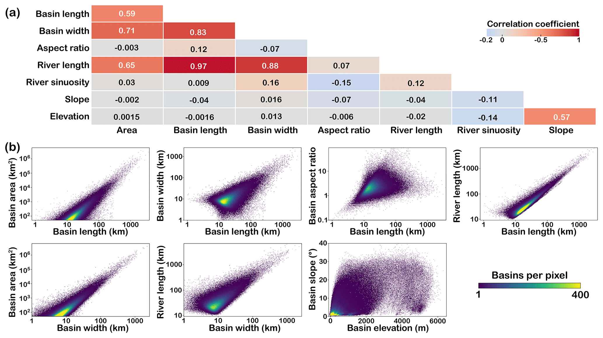
Figure 6The correlation among metrics. (a) Heatmap shows the linear correlation coefficients among eight metrics. The correlation coefficient indicates the extent and direction of the linear relationship between two variables. It ranges from −1 to 1, where positive values signify a positive correlation, with a higher absolute value indicating a stronger relationship. (b) A 2D density plot revealing relationships between selected metrics.
3.4 Hack's law
Hack's law is an empirical relationship that relates river length to basin area (Hack, 1957). It can be expressed as L=kAh, where L represents the length of the longest river measured from drainage divide to river mouth; A is drainage area; and k and h are the constant and exponent, respectively. Hack's law is a fundamental concept in geomorphology and hydrology, crucial for understanding river network dynamics. In addition, Hack's law derived from Earth can potentially be compared to valley systems on Mars, providing insights into its climates and hydrological processes (Luo et al., 2023; Penido et al., 2013; Som et al., 2009). Previous studies have obtained different values for k and h in Hack's law, which vary across regions. The k ranges from 1 to 5, while the range for h is typically 0.4–0.7 (Hack, 1957; Luo et al., 2023; Mueller, 1972; O'Malley, 2020; Sassolas-Serrayet et al., 2018; Yi et al., 2018). Recently, based on 3685 global catchments, Hack's law with an exponent of 0.56 was obtained (O'Malley, 2020).
Here, we utilized basin areas and river lengths in Basin90m to establish a new global Hack's law with k=2.1 km−0.08 and h=0.54 (Fig. 7). These values not only match regional case studies (Hack, 1957; He et al., 2021a; Montgomery and Dietrich, 1992; Sassolas-Serrayet et al., 2018; Yi et al., 2018; Yuan et al., 2023) but also align with results derived from global drainage systems (O'Malley, 2020).
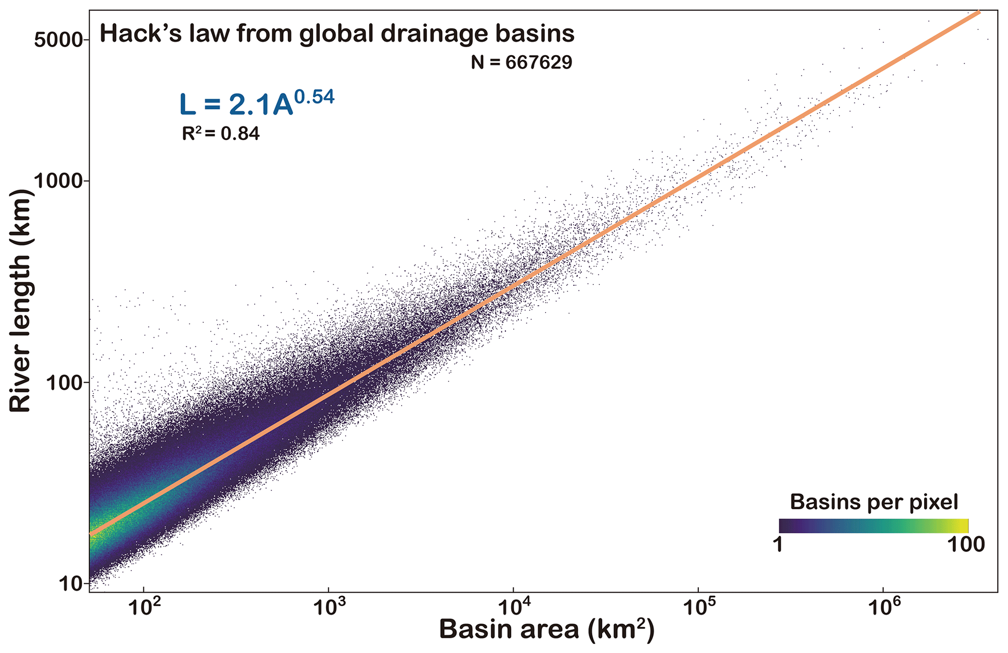
Figure 7Hack's law fitted based on basin area (A) and river length (L). We used all basins in Basin90m to fit Hack's law, including all stream orders.
Due to the absence of a published database for a direct comparison with the eight parameters contained in Basin90m, we used the Hydrology Tool in ArcGIS to extract the drainage divide and main channel of the Moche Basin in Peru. On this foundation, we validated the accuracy of the spatial position of the basin boundary and the longest river channel against HydroSHEDS (Lehner and Grill, 2013), the drainage system extracted by ArcGIS, and Google Earth images. We then compared the morphological metrics in Basin90m against HydroATLAS (Linke et al., 2019) and the measurements from ArcGIS. Furthermore, we selected 10 representative drainage basins spanning the North American continent to compare drainage areas with HydroATLAS. In addition, we discussed the limitations of Basin90m.
4.1 Spatial accuracy of drainage system
The accuracy of basin boundaries and river channels directly affects the calculation of the sizes and shapes of drainage systems. We used the Moche River basin in Peru as an example to verify the spatial accuracy of Basin90m because it contains diverse terrain features (Fig. 8a). Additionally, the presence of the Moche Civilization in the downstream plain of the Moche River indicates that human modification of the landscape has been ongoing for approximately 3000 years (Toyne et al., 2014). The Moche River originates in the Andes and flows into the Pacific Ocean. The Moche River basin encompasses an area of 2143 km2, with its highest altitude reaching 4257 m. Nearly half of the drainage basin is located in the upstream low-relief plateau. The middle reaches consist of a deep canyon that occupies 40 % of the area. The downstream area is a plain covering 10 % of the basin, and the river only decreases in elevation by 150 m over 20 km along the plain.
We compared the spatial accuracy of drainage systems in Basin90m with two datasets. The first one is HydroSHEDS, which consists of HydroRIVERS and HydroBASINS (Lehner and Grill, 2013). HydroSHEDS has a spatial resolution of 500 m and has been widely used in various fields such as geomorphology, hydrology, ecology, climatology, and geohazards (McEwan et al., 2023; Palmer et al., 2023; Tu et al., 2023). The second dataset we compare with Basin90m is the drainage system of the Moche Basin, which we extracted from ArcGIS using the same 90 m SRTM DEM (Farr et al., 2007). Due to the different DEM resolutions and methods in the three data items, the basins and rivers only partially overlap (Fig. 8a).
In the deep-canyon area (Fig. 8b), HydroRIVERS is coarse and does not match the river channel. In comparison, although Basin90m does not fully align with the actual river channel, there is a noticeable improvement in accuracy. The accuracy of the river extracted using ArcGIS falls between Basin90m and HydroRIVERS. The differences between the three are more pronounced in the plain (Fig. 8c). HydroRIVERS lies along the floodplain rather than the river channel. In contrast, even in such a low-relief area with human modifications, Basin90m follows the position of the river channel. The performance of the river obtained using ArcGIS falls between the two datasets.
We selected a segment of the drainage divide to compare the accuracy of the basin boundary (Fig. 8d). The drainage divide in Basin90m follows the ridge. However, HydroBASINS does not follow the ridge and even cuts through a deeply incised river channel. Although the drainage divide extracted using ArcGIS generally follows the ridge, it is not as accurate as Basin90m. In summary, Basin90m exhibits a higher spatial accuracy in the Moche Basin than HydroSHEDS and drainage systems extracted using ArcGIS.
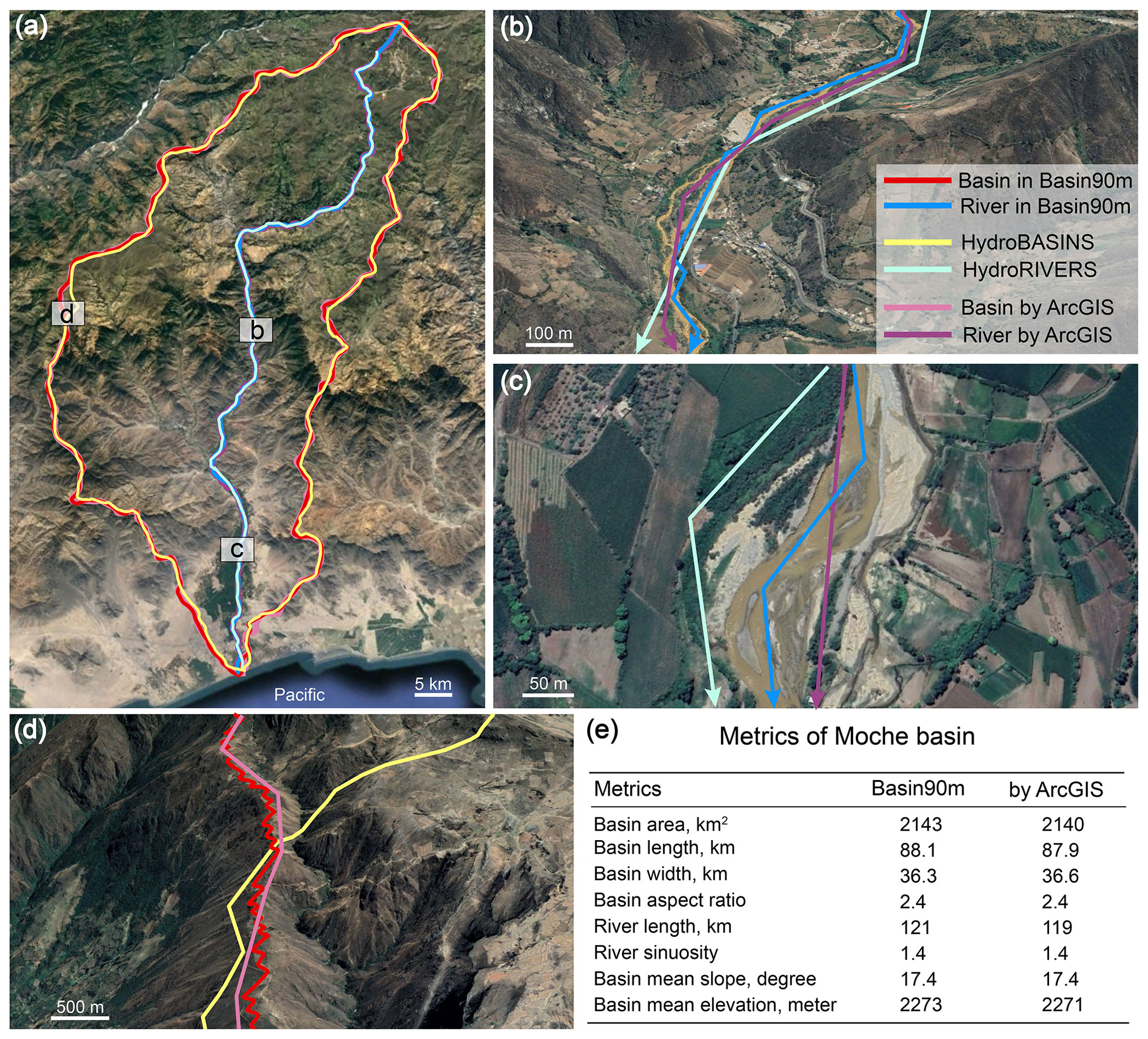
Figure 8Spatial accuracy of the drainage system in Basin90m compared against HydroSHEDS (Lehner and Grill, 2013), drainage systems extracted by ArcGIS, and © Google Earth images. The Moche Basin in Peru serves as an example that simultaneously combines a low-relief plateau, deep canyons, and farming land in plains. (a) The drainage system of the Moche Basin. A comparison between river channels in a deep-canyon region (b) and a flat region (c). (d) A comparison between drainage divides. (e) A comparison of the metrics for the Moche Basin between Basin90m and those extracted by ArcGIS.
4.2 Accuracy of morphological metrics
The morphological metrics that can be directly compared between the published databases and Basin90m only include basin area, slope, and elevation. For example, in HydroATLAS (Linke et al., 2019), the area, slope, and elevation of the Moche Basin are 2125 km2, 17°, and 2267 m, respectively. This means the difference between Basin90m and HydroATLAS in the Moche Basin is less than 1 %. To validate the accuracy of the remaining five parameters included in Basin90m, we used the results of the Moche Basin extracted by ArcGIS.
The primary difference in the extraction of drainage systems between ArcGIS and our TopoToolbox script is in the handling of local minimums. ArcGIS uses the filling method, which fills depressions. In TopoToolbox, we used the carving method, which carves a channel through local depressions to allow the river to flow out. Therefore, although both used the same DEM, there are still slight differences in the positions of the drainage systems (Fig. 8a–d). Except for a 1.6 % difference in river length, all seven remaining parameters exhibit variances of less than 0.8 %. Basin90m's river channel and drainage divide are more elaborate than those extracted by ArcGIS (Fig. 8b–d), resulting in longer channels. Therefore, in the Moche Basin, Basin90m has a higher spatial accuracy (Fig. 8b–d) and provides accurate values for the morphometric metrics (Fig. 8e).
4.3 Accuracy of basin area
Drainage area is an important metric to evaluate the accuracy of drainage basin delineation. We compared drainage areas in Basin90m with those in HydroATLAS (Linke et al., 2019). We selected 10 basins across the USA for comparison (Fig. 9a). These drainage basins are evenly distributed in the east–west direction across the North American continent, thus spanning diverse geological regimes, terrains, climates, and vegetation environments. Basins 1–5 are located in the west, with an arid climate, steep topography, and relatively active tectonics. Basins 6–10 are located in the east, with low topographic relief but more precipitation and vegetation.
Due to the difference in DEM resolution (90 m for Basin90m and 500 m for HydroATLAS) and in algorithms for delineating basin boundaries, the drainage divides from the two databases do not always coincide (Fig. 9b). However, the two databases are consistent without substantial discrepancies (Fig. 9c). We quantified their difference using absolute relative error. The absolute relative error is the absolute value of the area difference between Basin90m and HydroATLAS as a ratio to HydroATLAS. Smaller values indicate higher agreement between the two datasets. Except for a 1.2 % absolute relative error for basin 4, the values for the other nine basins are below 0.8 %. The average absolute relative error for the 10 basins is 0.47 % (Fig. 9c). This slight discrepancy is acceptable given the nearly 5-fold difference in DEM resolution and variations in algorithms for basin delineation.
In summary, the validation results based on the Peruvian Moche River basin and 10 representative basins across the USA indicate that Basin90m has a high resolution for basin boundaries and river channels. Besides this, the morphological parameters exhibit high accuracy.
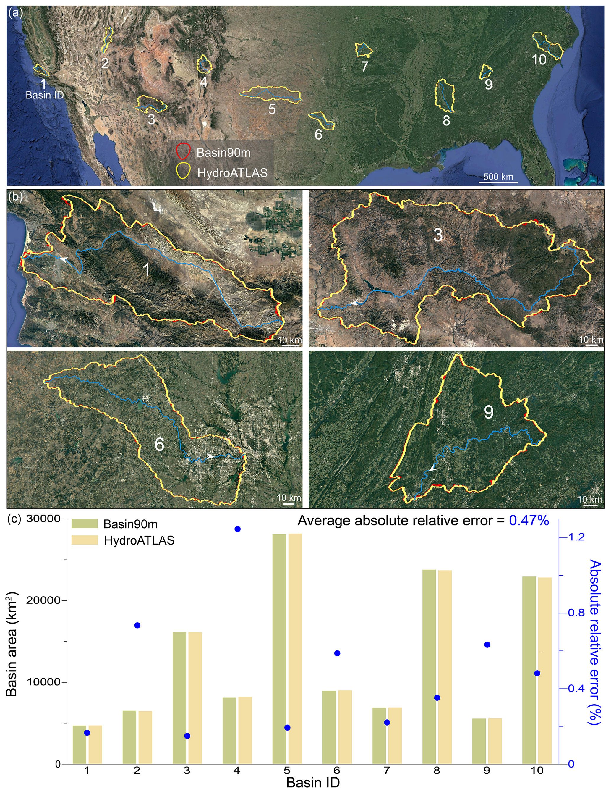
Figure 9The accuracy of basin area in Basin90m, compared against HydroATLAS (Linke et al., 2019). The stream order for all 10 of the representative drainage basins is 4. (a) © Google Earth image shows 10 example drainage basins in the USA. (b) Enlarged images of four representative basins. Basin 1 has an ocean outlet. Basin 3 is situated in a high-altitude arid region. Basin 6 features a flat terrain and encompasses a major city (Dallas). Basin 9 is located in a tectonically active folded region. (c) Comparison of basin areas between Basin90m and HydroATLAS.
4.4 Limitations
Although Basin90m has improved spatial accuracy of drainage systems compared to HydroSHEDS, it still has some limitations. First, the basins and rivers in Basin90m are entirely based on DEM analysis. Therefore, the measurement and processing errors of the DEM itself can affect the spatial accuracy of Basin90m. Second, in nature, rivers can flow in any direction. However, the D8 method was used to calculate flow direction, which reduces computational complexity but limits the flow to only eight directions. Third, after obtaining 667 629 global basins and their longest rivers, no manual removal of false rivers has been conducted, especially in flat areas. Users must consider these limitations when using and interpreting the results of Basin90m, particularly in flat areas with severe human modifications.
Basin90m is freely available at https://doi.org/10.5880/GFZ.4.6.2023.004 (He et al., 2023). Basin90m contains 667 629 drainage basins with areas over 50 km2. Each basin is accompanied by its longest river channel, from drainage divide to river mouth. Basins and rivers are stored in Esri shapefile format, which can be opened and edited using GIS software (e.g., QGIS and ArcGIS) and Python libraries (e.g., GeoPandas).
The data are grouped by six continents. Each continent contains multiple stream orders. For example, the European basin files consist of eight shapefiles corresponding to stream orders 1–8. The filenames of basins and rivers include the stream order and continent information. For instance, Africa_Basin_5.shp contains all African basins with a stream order of 5. The eight parameters describing the size and shape of drainage systems (Fig. 2c) were stored in the attribute tables of basin shapefiles. The shapefiles for global basins and rivers are 7.8 and 2.5 GB, respectively. The attribute tables of all global basins were merged into a single Excel file (Basin90m.xlsx).
The MATLAB script (Basin90m.m) used to generate Basin90m and a user guide are freely available at https://doi.org/10.5880/GFZ.4.6.2023.004 (He et al., 2023). Note that, before running this code, one needs to install TopoToolbox (Schwanghart and Scherler, 2014). The link https://topotoolbox.wordpress.com/topotoolbox/ (last access: 14 February 2024) provides installation and usage instructions for TopoToolbox.
We present Basin90m, a global dataset of the shape of drainage systems. Utilizing a 90 m resolution DEM, we extracted 667 629 drainage basins with an area over 50 km2. Each basin contains one river channel, extending from the upstream drainage divide to the downstream river mouth. Basin90m provides information on the size, shape, hierarchy, and topography of drainage basins, as well as the length and sinuosity of river channels. Compared to the published datasets, Basin90m offers a higher resolution, includes the shape of basins and rivers, and excludes drainage systems with over half of their area located in lakes or sandy deserts.
We presented the variations among different stream orders in terms of the quantity, size, and shape of drainage systems. The number of basins decreased from 521 857 for the first order to 3 for the ninth order. In contrast, increasing stream order raised the average basin area, river length, and sinuosity. We displayed the probability and spatial distribution of the eight parameters. The most notable feature is that numerous narrow and steep basins are distributed in the margins of the Tibetan Plateau. We then demonstrated the correlations among the eight parameters. The highest correlation coefficient of 0.97 was found between basin length and river length, indicating the coevolution of rivers and basins in nature. Using the basin area and river length from Basin90m, we fitted a global Hack's law as L=2.1A0.54.
To validate the accuracy of Basin90m, we compared it with multiple data sources using the Moche Basin in Peru and 10 drainage basins across the North American continent as examples. The data compared with Basin90m include basin boundaries, river locations, and river lengths provided by HydroSHEDS; basin area, slope, and elevation from HydroATLAS; basin and river locations from Google Earth images; and basin boundaries and area, river locations and lengths, and drainage system shape metrics extracted using ArcGIS. The results showed that Basin90m exhibited the highest spatial accuracy. Furthermore, the difference in terms of morphological parameters between Basin90m and other data sources is typically less than 1 %. These validations confirm the accuracy of Basin90m as a valuable resource for analyzing drainage systems on a local or global scale.
CH, CJY, and JMT conceived the initial idea. CH performed calculations and data processing, wrote a first draft, and made the figures. CJY built the code to extract Basin90m from DEM, with inputs from RFO. JMT designed the method for measuring the length and width of drainage basins. RFO collected the global DEM. GSdQ proposed using the aridity index to classify sandy deserts. JB, HT, SG, and XY participated in data processing and analysis. All authors contributed to the conceptualization, discussion, data collection, and editing of all the components of Basin90m and this paper.
The contact author has declared that none of the authors has any competing interests.
Publisher’s note: Copernicus Publications remains neutral with regard to jurisdictional claims made in the text, published maps, institutional affiliations, or any other geographical representation in this paper. While Copernicus Publications makes every effort to include appropriate place names, the final responsibility lies with the authors.
We appreciate the high-performance computing team at the German Research Centre for Geosciences (GFZ) for their technical support. We thank Kirsten Elger from the GFZ Library and Information Services for the help in uploading and managing Basin90m data in GFZ Data Services. We thank Gareth Roberts and Jingtao Lai for the discussions.
Chuanqi He received funding from the NSFC (National Natural Science Foundation of China) (grant no. 42201008) and the Helmholtz-OCPC postdoc program (grant no. 202120). Xiaoping Yuan received funding from the NSFC (grant no. 42272261). Open-access funding was enabled and organized by Project DEAL.
The article processing charges for this open-access publication were covered by the Helmholtz Centre Potsdam – GFZ German Research Centre for Geosciences.
This paper was edited by Yuanzhi Yao and reviewed by Polina Lemenkova and one anonymous referee.
Allen, G. H. and Pavelsky, T. M.: Global extent of rivers and streams, Science, 361, 585–588, https://doi.org/10.1126/science.aat0636, 2018.
Amatulli, G., Garcia Marquez, J., Sethi, T., Kiesel, J., Grigoropoulou, A., Üblacker, M. M., Shen, L. Q., and Domisch, S.: Hydrography90m: a new high-resolution global hydrographic dataset, Earth Syst. Sci. Data, 14, 4525–4550, https://doi.org/10.5194/essd-14-4525-2022, 2022.
Bennett, S. J. and Liu, R.: Basin self-similarity, Hack's law, and the evolution of experimental rill networks, Geology, 44, 35–38, https://doi.org/10.1130/G37214.1, 2016.
Biron, P. M., Buffin-Belanger, T., Larocque, M., Chone, G., Cloutier, C. A., Ouellet, M. A., Demers, S., Olsen, T., Desjarlais, C., and Eyquem, J.: Freedom space for rivers: a sustainable management approach to enhance river resilience, Environ. Manage., 54, 1056–1073, https://doi.org/10.1007/s00267-014-0366-z, 2014.
Castelltort, S., Goren, L., Willett, S. D., Champagnac, J.-D., Herman, F., and Braun, J.: River drainage patterns in the New Zealand Alps primarily controlled by plate tectonic strain, Nat. Geosci., 5, 744–748, https://doi.org/10.1038/ngeo1582, 2012.
Cook, K. L., Rekapalli, R., Dietze, M., Pilz, M., Cesca, S., Rao, N. P., Srinagesh, D., Paul, H., Metz, M., Mandal, P., Suresh, G., Cotton, F., Tiwari, V. M., and Hovius, N.: Detection and potential early warning of catastrophic flow events with regional seismic networks, Science, 374, 87–92, https://doi.org/10.1126/science.abj1227, 2021.
Datry, T., Boulton, A. J., Fritz, K., Stubbington, R., Cid, N., Crabot, J., and Tockner, K.: Non-perennial segments in river networks, Nat. Rev. Earth Environ., 4, 815–830, https://doi.org/10.1038/s43017-023-00495-w, 2023.
Farr, T. G., Rosen, P. A., Caro, E., Crippen, R., Duren, R., Hensley, S., Kobrick, M., Paller, M., Rodriguez, E., Roth, L., Seal, D., Shaffer, S., Shimada, J., Umland, J., Werner, M., Oskin, M., Burbank, D., and Alsdorf, D.: The Shuttle Radar Topography Mission, Rev. Geophys., 45, RG2004, https://doi.org/10.1029/2005RG000183, 2007.
Gamo, M., Shinoda, M., and Maeda, T.: Classification of arid lands, including soil degradation and irrigated areas, based on vegetation and aridity indices, Int. J. Remote Sens., 34, 6701–6722, https://doi.org/10.1080/01431161.2013.805281, 2013.
Guth, P. L.: Drainage basin morphometry: a global snapshot from the shuttle radar topography mission, Hydrol. Earth Syst. Sci., 15, 2091–2099, https://doi.org/10.5194/hess-15-2091-2011, 2011.
Habousha, K., Goren, L., Nativ, R., and Gruber, C.: Plan-form evolution of drainage basins in response to tectonic changes: Insights from experimental and numerical landscapes, J. Geophys. Res.-Earth, 128, e2022JF006876, https://doi.org/10.1029/2022JF006876, 2023.
Hack, J. T.: Studies of longitudinal stream profiles in Virginia and Maryland, United States Geological Survey, https://pubs.usgs.gov/pp/0294b/report.pdf (last access: 14 February 2024), 1957.
He, C., Yang, C. J., Turowski, J. M., Rao, G., Roda-Boluda, D. C., and Yuan, X. P.: Constraining tectonic uplift and advection from the main drainage divide of a mountain belt, Nat. Commun., 12, 544, https://doi.org/10.1038/s41467-020-20748-2, 2021a.
He, C., Yang, C. J., Rao, G., Roda-Boluda, D. C., Yuan, X. P, Yang, R., Gao, L., and Zhang, L.: Landscape response to normal fault linkage: Insights from numerical modeling, Geomorphology, 388, 107796, https://doi.org/10.1016/j.geomorph.2021.107796, 2021b.
He, C., Yang, C. J., Turowski, J. M., Ott, R. F., Braun, J., Tang, H., Ghantous, S., Yuan, X. P., and Stucky de Quay, G.: Basin90m, a new global drainage basin dataset, GFZ Data Services [code and data set], https://doi.org/10.5880/GFZ.4.6.2023.004, 2023.
He, C., Braun, J., Tang, H., Yuan, X. P., Acevedo-Trejos, E., Ott, R. F., and Stucky de Quay, G.: Drainage divide migration and implications for climate and biodiversity, Nat. Rev. Earth Environ., https://doi.org/10.1038/s43017-023-00511-z, 2024.
Hou, J., Van Dijk, A. I. J. M., Renzullo, L. J., and Larraondo, P. R.: GloLakes: water storage dynamics for 27 000 lakes globally from 1984 to present derived from satellite altimetry and optical imaging, Earth Syst. Sci. Data, 16, 201–218, https://doi.org/10.5194/essd-16-201-2024, 2024.
Ielpi, A., Lapôtre, M. G. A., Finotello, A., and Roy-Léveillée, P.: Large sinuous rivers are slowing down in a warming Arctic, Nat. Clim. Change, 13, 375–381, https://doi.org/10.1038/s41558-023-01620-9, 2023.
Kirchner, J. W., Feng, X., and Neal, C.: Catchment-scale advection and dispersion as a mechanism for fractal scaling in stream tracer concentrations, J. Hydrol., 254, 82–101, https://doi.org/10.1016/S0022-1694(01)00487-5, 2001.
Lehner, B. and Grill, G.: Global river hydrography and network routing: baseline data and new approaches to study the world's large river systems, Hydrol. Process., 27, 2171–2186, https://doi.org/10.1002/hyp.9740, 2013.
Lehner, B., Verdin, K., and Jarvis, A.: New global hydrography derived from spaceborne elevation data, Eos, Trans., Am. Geophys. Union, 89, 93–104, https://doi.org/10.1029/2008EO100001, 2008.
Lin, P., Pan, M., Wood, E. F., Yamazaki, D., and Allen, G. H.: A new vector-based global river network dataset accounting for variable drainage density, Sci. Data, 8, 28, https://doi.org/10.1038/s41597-021-00819-9, 2021.
Lindsay, J. B.: Efficient hybrid breaching-filling sink removal methods for flow path enforcement in digital elevation models, Hydrol. Process., 30, 846–857, https://doi.org/10.1002/hyp.10648, 2016.
Linke, S., Lehner, B., Ouellet Dallaire, C., Ariwi, J., Grill, G., Anand, M., Beames, P., Burchard-Levine, V., Maxwell, S., Moidu, H., Tan, F., and Thieme, M.: Global hydro-environmental sub-basin and river reach characteristics at high spatial resolution, Sci. Data, 6, 283, https://doi.org/10.1038/s41597-019-0300-6, 2019.
Luo, W., Howard, A. D., Craddock, R. A., Oliveira, E. A., and Pires, R. S.: Global spatial distribution of Hack's Law exponent on Mars consistent with early arid climate, Geophys. Res. Lett., 50, e2022GL102604, https://doi.org/10.1029/2022GL102604, 2023.
Mantilla, R., Troutman, B. M., and Gupta, V. K.: Testing statistical self-similarity in the topology of river networks, J. Geophys. Res., 115, F03038, https://doi.org/10.1029/2009JF001609, 2010.
Masutomi, Y., Inui, Y., Takahashi, K., and Matsuoka, Y.: Development of highly accurate global polygonal drainage basin data, Hydrol. Process., 23, 572–584, https://doi.org/10.1002/hyp.7186, 2009.
Matthews, W. J. and Robison, H. W.: Influence of drainage connectivity, drainage area and regional species richness on fishes of the interior highlands in Arkansas, Am. Midl. Nat., 139, 1–19, https://doi.org/10.1674/0003-0031(1998)139[0001:IODCDA]2.0.CO;2, 1998.
Maurer, J. M., Schaefer, J. M., Russell, J. B., Rupper, S., Wangdi, N., Putnam, A. E., and Young, N.: Seismic observations, numerical modeling, and geomorphic analysis of a glacier lake outburst flood in the Himalayas, Sci. Adv., 6, eaba3645, https://doi.org/10.1126/sciadv.aba3645, 2020.
McEwan, E., Stahl, T., Howell, A., Langridge, R., and Wilson, M.: Coseismic river avulsion on surface rupturing faults: Assessing earthquake-induced flood hazard, Science, 9, eadd2932, https://doi.org/10.1126/sciadv.add2932, 2023.
Messager, M. L., Lehner, B., Grill, G., Nedeva, I., and Schmitt, O.: Estimating the volume and age of water stored in global lakes using a geo-statistical approach, Nat. Commun., 7, 13603, https://doi.org/10.1038/ncomms13603, 2016.
Montgomery, D. R. and Dietrich, W. E.: Channel initiation and the problem of landscape scale, Science, 255, 826–830, https://doi.org/10.1126/science.255.5046.826, 1992.
Mueller, J. E.: Re-evaluation of the relationship of master streams and drainage basins, Geol. Soc. Am. Bull., 83, 3471–3474, https://doi.org/10.1130/0016-7606(1972)83[3471:ROTROM]2.0.CO;2, 1972.
Nagayama, S. and Nakamura, F.: The significance of meandering channel to habitat diversity and fish assemblage: a case study in the Shibetsu River, northern Japan, Limnology, 19, 7–20, https://doi.org/10.1007/s10201-017-0512-4, 2017.
O'Malley, C. P. B.: Quantitative analysis of river profiles and fluvial landscapes, PhD thesis, University of Cambridge, https://doi.org/10.17863/CAM.51663, 2020.
Palmer, P. I., Wainwright, C. M., Dong, B., Maidment, R. I., Wheeler, K. G., Gedney, N., Hickman, J. E., Madani, N., Folwell, S. S., Abdo, G., Allan, R. P., Black, E. C. L., Feng, L., Gudoshava, M., Haines, K., Huntingford, C., Kilavi, M., Lunt, M. F., Shaaban, A., and Turner, A. G.: Drivers and impacts of Eastern African rainfall variability, Nat. Rev. Earth Environ., 4, 254–270, https://doi.org/10.1038/s43017-023-00397-x, 2023.
Penido, J. C., Fassett, C. I., and Som, S. M.: Scaling relationships and concavity of small valley networks on Mars, Planet. Space Sci., 75, 105–116, https://doi.org/10.1016/j.pss.2012.09.009, 2013.
Rhoads, B. L., Schwartz, J. S., and Porter, S.: Stream geomorphology, bank vegetation, and three-dimensional habitat hydraulics for fish in midwestern agricultural streams, Water Resour. Res., 39, 1218, https://doi.org/10.1029/2003WR002294, 2003.
Sassolas-Serrayet, T., Cattin, R., and Ferry, M.: The shape of watersheds, Nat. Commun., 9, 3791, https://doi.org/10.1038/s41467-018-06210-4, 2018.
Schwanghart, W., Groom, G., Kuhn, N. J., and Heckrath, G.: Flow network derivation from a high resolution DEM in a low relief, agrarian landscape, Earth Surf. Process. Landf., 38, 1576–1586, https://doi.org/10.1002/esp.3452, 2013.
Schwanghart, W. and Scherler, D.: Bumps in river profiles: uncertainty assessment and smoothing using quantile regression techniques, Earth Surf. Dynam., 5, 821–839, https://doi.org/10.5194/esurf-5-821-2017, 2017.
Schwanghart, W. and Scherler, D.: Short Communication: TopoToolbox 2 – MATLAB-based software for topographic analysis and modeling in Earth surface sciences, Earth Surf. Dynam., 2, 1–7, https://doi.org/10.5194/esurf-2-1-2014, 2014.
Shelef, E.: Channel profile and plan-view controls on the aspect ratio of river basins, Geophys. Res. Lett., 45, 11712–11721, https://doi.org/10.1029/2018GL080172, 2018.
Shen, X., Anagnostou, E. N., Mei, Y., and Hong, Y.: A global distributed basin morphometric dataset, Sci. Data, 4, 160124, https://doi.org/10.1038/sdata.2016.124, 2017.
Sikder, M. S., Wang, J., Allen, G. H., Sheng, Y., Yamazaki, D., Song, C., Ding, M., Crétaux, J.-F., and Pavelsky, T. M.: Lake-TopoCat: a global lake drainage topology and catchment database, Earth Syst. Sci. Data, 15, 3483–3511, https://doi.org/10.5194/essd-15-3483-2023, 2023.
Som, S. M., Montgomery, D. R., and Greenberg, H. M.: Scaling relations for large Martian valleys, J. Geophys. Res., 114, E02005, https://doi.org/10.1029/2008JE003132, 2009.
Sreedevi, P. D., Owais, S., Khan, H. H., and Ahmed, S.: Morphometric analysis of a watershed of South India using SRTM data and GIS, J. Geol. Soc. India, 73, 543–552, https://doi.org/10.1007/s12594-009-0038-4, 2009.
Strahler, A. N.: Quantitative analysis of watershed geomorphology, Eos, Trans., Am. Geophys. Union, 38, 913–920, https://doi.org/10.1029/TR038i006p00913, 1957.
Strong, C. M. and Mudd, S. M.: Explaining the climate sensitivity of junction geometry in global river networks, P. Natl. Acad. Sci. USA, 119, e2211942119, https://doi.org/10.1073/pnas.2211942119, 2022.
Tarboton, D. G.: A new method for the determination of flow directions and upslope areas in grid digital elevation models, Water Resour. Res., 33, 309–319, https://doi.org/10.1029/96WR03137, 1997.
Toyne, J. M., White, C. D., Verano, J. W., Uceda Castillo, S., Millaire, J. F., and Longstaffe, F. J.: Residential histories of elites and sacrificial victims at Huacas de Moche, Peru, as reconstructed from oxygen isotopes, J. Archaeol. Sci., 42, 15–28, https://doi.org/10.1016/j.jas.2013.10.036, 2014.
Tu, T., Comte, L., and Ruhi, A.: The color of environmental noise in river networks, Nat. Commun., 14, 1728, https://doi.org/10.1038/s41467-023-37062-2, 2023.
USGS: HYDRO1k elevation derivative database, U.S. Geol. Surv., https://doi.org/10.5066/F77P8WN0, 2000.
Verdin, K. L.: Hydrologic derivatives for modeling and applications (HDMA) database-A new global high-resolution database, U.S. Geol. Surv., Virginia, https://doi.org/10.3133/ds1053, 2017.
Vörösmarty, C. J., Fekete, B. M., Meybeck, M., and Lammers, R. B.: Global system of rivers: Its role in organizing continental land mass and defining land-to-ocean linkages, Global Biogeochem. Cy., 14, 599–621, https://doi.org/10.1029/1999GB900092, 2000.
Yan, D., Li, C., Zhang, X., Wang, J., Feng, J., Dong, B., Fan, J., Wang, K., Zhang, C., Wang, H., Zhang, J., and Qin, T.: A data set of global river networks and corresponding water resources zones divisions v2, Sci. Data, 9, 770, https://doi.org/10.1038/s41597-019-0243-y, 2022.
Yi, R. S., Arredondo, Á., Stansifer, E., Seybold, H., and Rothman, D. H.: Shapes of river networks, Proc. R. Soc. A 474, 20180081, https://doi.org/10.1098/rspa.2018.0081, 2018.
Yu, Z., Zhang, J., Wang, H., Zhao, J., Dong, Z., Peng, W., and Zhao, X.: Quantitative analysis of ecological suitability and stability of meandering rivers, Front. Biosci. Landmark, 27, 42, https://doi.org/10.31083/j.fbl2702042, 2022.
Yuan, X. P., Jiao, R., Liu-Zeng, J., Dupont-Nivet, G., Wolf, S. G., and Shen, X.: Downstream propagation of fluvial erosion in Eastern Tibet, Earth Planet. Sc. Lett., 605, 118017, https://doi.org/10.1016/j.epsl.2023.118017, 2023.
Zomer, R. J., Xu, J., and Trabucco, A.: Version 3 of the Global Aridity Index and Potential Evapotranspiration Database, Sci. Data, 9, 409, https://doi.org/10.1038/s41597-022-01493-1, 2022.