3D reconstruction of horizontal and vertical quasi-geostrophic currents in the North Atlantic Ocean

In this paper we introduce a new high-resolution ($\mathrm{1}/\mathrm{10}$°) data-driven dataset of 3D ocean currents developed by the National Research Council of Italy in the framework of the European Space Agency World Ocean Circulation project: the WOC-NATL3D dataset. The product domain extends over a wide portion of the North Atlantic Ocean from the surface down to 1500 m depth, and the dataset covers the period between 2010 and 2019. To generate this product, a diabatic quasi-geostrophic diagnostic model is applied to data-driven 3D temperature and salinity fields obtained through a deep learning technique, along with ERA5 fluxes and empirical estimates of the horizontal Ekman currents based on input provided by the European Copernicus Marine Service. The assessment of WOC-NATL3D currents is performed by direct validation of the total horizontal velocities with independent drifter estimates at various depths (0, 15 and 1000 m) and by comparing them with existing reanalyses that are obtained through the assimilation of observations into ocean general circulation numerical models. Our estimates of the ageostrophic components of the flow improve the total horizontal velocity reconstruction, being more accurate and closer to observations than model reanalyses in the upper layers, also providing an indirect proof of the reliability of the resulting vertical velocities. The reconstructed WOC-NATL3D currents are freely available at https://doi.org/10.12770/0aa7daac-43e6-42f3-9f95-ef7da46bc702 (Buongiorno Nardelli, 2022).

1 Introduction

As a key component of Earth's climate system, the ocean plays a critical role in regulating global climate patterns, but we see its marine environment increasingly being impacted by climate change, with far-reaching consequences on various ecological processes and organisms (e.g., Poloczanska et al., 2013; Doney et al., 2012). Changes in sea surface temperatures, ocean currents and precipitation patterns are disrupting the delicate balance of marine ecosystems, resulting in shifts in habitat distribution and migration patterns, alterations in nutrient availability, and changes in the physical and chemical properties of seawater (Constable et al., 2014; van Gennip et al., 2017; Du et al., 2019).

In this context, many uncertainties persist regarding the factors influencing fish ecology and abundance, beyond fishing pressure. These include uncertainties surrounding the change in oceanic currents, which can affect the distribution of spawning areas; the survival and dispersal of larvae; and the availability of food for larvae, juveniles and adult fishes, as well as their migratory behaviors. Additionally, the drivers and patterns of variability and diversity among planktonic organisms, which are essential in the marine ecosystem and directly impact higher trophic levels, remain poorly understood (Ibarbalz et al., 2019).

In many cases, high-resolution data are needed to correctly account for relevant dynamical regimes, especially when transport and dispersion processes are expected to be dominant. To demonstrate how innovative approaches can contribute to address these fundamental gaps in knowledge and to enhance scientific advice for fishery management, the European Space Agency included a specific “Theme” dedicated to “Sustainable fisheries” within its World Ocean Circulation (WOC) project (http://www.worldoceancirculation.org, last access: 22 July 2023). Specifically, in the framework of WOC, new methodologies have been proposed to combine satellite data, in situ measurements, atmospheric forcings, and diagnostic models, in order to obtain high-spatial-resolution (mesoscale-resolving) estimates of the 3D currents (including its vertical component), to be used for specific case studies.

Actually, direct in situ measurements of ocean currents are still quite limited, and, due to its small magnitude, measurements of the vertical velocity remain one of the biggest challenges in oceanography (Tarry et al., 2021; Comby et al., 2022). Vertical velocities are therefore generally inferred indirectly, and a common approach to diagnose them is to use the quasi-geostrophic omega equation (Tintoré et al., 1991; Giordani et al., 2006; Canuto and Cheng, 2017; Qiu et al., 2020).

Within WOC, a daily 3D ocean current product has been developed, including the vertical component, at a mesoscale-resolving spatial resolution ($\mathrm{1}/\mathrm{10}\mathit{°}\times \mathrm{1}/\mathrm{10}\mathit{°}$). This product covers a wide section of the central/North Atlantic Ocean (20–50° N, 6–76° W). The chosen domain encompasses the Eastern Boundary Upwelling Systems along the African and Iberian coasts, which serve as important fishing grounds for several species significant for both local communities and commercial exploitation (Kämpf and Chapman, 2016). It also includes the Sargasso Sea, the exclusive location where threatened European and American eels reproduce (Dekker, 2019), and the Gulf Stream area. This entire domain holds immense importance for fishery activities and is identified as a key area within international conventions for the conservation of fishing resources, such as tuna and tuna-like fishes under ICCAT (International Commission for the Conservation of Atlantic Tunas). Prototypal WOC-NATL3D data have been already used to investigate the role of the 3D dispersion of eels' larvae from the Sargassum towards the European coasts (Munk et al., 2023). Specifically, Lagrangian drift trajectories were simulated starting from our data-driven high-resolution reconstruction of the 3D flow, based on the eels' larvae data collected during targeted surveys. Focusing on the effects of mesoscale processes, Munk et al. (2023) found that, while eels' spawning area is delimited by temperature and salinity fronts, their dispersion patterns are mostly influenced by current shear and eddy strain, with a significant dispersal towards the northeast. This result is supported by historical data, challenging common interpretations that assume a dominant initial westward advection of the entire population toward the Gulf Stream.

Building on recent work carried out in the framework of the European Copernicus Service – Multi Observations Thematic Assembly Center to develop the OMEGA3D product (Buongiorno Nardelli, 2020b), the new WOC-NATL3D product has been obtained by solving a diabatic Q vector formulation of the quasi-geostrophic version of the omega equation (Buongiorno Nardelli et al., 2018; Giordani et al., 2006), whose vertical mixing terms are estimated by combining a modified version of the K-profile parameterization (KPP; Smyth et al., 2002) and empirical values based on a simplified Ekman dynamics parameterization. Once the omega equation is solved, horizontal ageostrophic components are also estimated.

The purpose of this paper is to provide an evaluation of 3D reconstruction of the quasi-geostrophic horizontal and vertical currents from this new North Atlantic data-driven 3D Currents product (WOC-NATL3D hereafter). The dataset achieves a daily resolution and is computed on a $\mathrm{1}/\mathrm{10}\mathit{°}\times \mathrm{1}/\mathrm{10}\mathit{°}$ horizontal resolution grid, over 75 unevenly spaced vertical levels (denser close to the surface), between the surface and 1500 m depth. It covers a wide part of the North Atlantic basin and spans 2010 to 2019. This time period was defined following the specifications of the ESA World Ocean Circulation project, with particular consideration given to the launch of the SMOS satellite in 2010. This product provides as well a 3D reconstruction of daily temperature and salinity, which is not addressed hereafter as it has been fully detailed in Buongiorno Nardelli (2020a). WOC-NATL3D is openly distributed by Ifremer/CERSAT through the project web page at https://www.worldoceancirculation.org/Products#/metadata/0aa7daac-43e6-42f3-9f95-ef7da46bc702 (last access: 24 October 2023).

The paper is organized as follows: Sect. 2 describes the input datasets and the one used for the evaluation of the production. The long short-term memory network and 3D current methods are also defined in this section. Direct comparison of the vertical velocity and the reconstruction performance is assessed in Sect. 3. Data availability is described in Sect. 4. Finally, the results are discussed and summarized in Sect. 5.

2 Data and methods

2.1 Input datasets

2.1.1 Reconstructed 3D tracer fields

The density field is necessary to solve the omega equation. Even if full details on the 3D reconstruction used within WOC-NATL3D processing chain are given in Buongiorno Nardelli (2020a), we recall here the main processing steps. A deep learning technique based on a long short-term memory network (LSTM) is used to optimize the reconstruction of 3D temperature and salinity fields. Then, the density, necessary to solve the omega equation, is deduced through the standard UNESCO formula. This 2D-to-3D processing requires 2D input fields of sea surface temperature (SST), sea surface salinity (SSS), absolute dynamic topography (ADT), and vertical profiles of temperature and salinity from in situ sensors and climatological 3D fields, described below:

• Sea surface temperature. SST data are from the L4 multi-year reprocessed Operational Sea Surface Temperature and Sea Ice Analysis (OSTIA), developed by the UK Met Office and distributed by the European Copernicus Marine Environment Monitoring Service (Copernicus, product ID:SST_GLO_SST_L4_REP_OBSERVATIONS_010_011). OSTIA combines and interpolates in situ observations from HadIOD and data (ESA SST CCI, C3S, EUMETSAT and REMSS) to provide global daily gap-free maps of foundation SST (i.e., values that are not affected by the diurnal cycle) and ice concentration at $\mathrm{1}/\mathrm{20}$° horizontal grid resolution. The OSTIA SST considered here covers the period 2010–2019 and was sub-sampled to $\mathrm{1}/\mathrm{10}$° resolution, by simply selecting one point out of two. The resulting grid is taken as the final grid used for the pre-processing of the other surface datasets.

• Sea surface salinity. SSS data were obtained by adapting the multidimensional optimal interpolation algorithm used within the Copernicus Marine Service (Buongiorno Nardelli et al., 2016; Droghei et al., 2016; Sammartino et al., 2022) to retrieve the global SSS product (product ID: MULTIOBS_GLO_PHY_S_SURFACE_MYNRT_015_013) to a daily processing over the $\mathrm{1}/\mathrm{10}$° North Atlantic grid. The technique is able to increase the effective resolution of the interpolated SSS by taking advantage of its covariance with local SST patterns in the open ocean. Copernicus weekly SSS fields (taken for from 2010 to 2019) were linearly interpolated in time between the two nearest analysis dates in order to obtain a daily background. A cubic-spline-interpolation method (Buongiorno Nardelli et al., 2012) was used to up-size the grid resolution of the weekly first guess field from $\mathrm{1}/\mathrm{4}$ to $\mathrm{1}/\mathrm{10}$°. Combined satellite and in situ SSS observations were then interpolated on a daily basis including information from OSTIA SST in the computation of the weights.

• Absolute dynamic topography. Using the dataset of optimal currents described in Buongiorno Nardelli and Ciani (2022) (see their Sect. 2.4) and based on Ciani et al. (2020), a new ADT product (WOC-NATL2D) is built (see their Sect. 2.5). Before being used as input to the LSTM model, an additional processing step is performed in order to make them coherent with in situ steric heights. Based on Buongiorno Nardelli et al. (2017), the ADT is adjusted by applying a linear regression between in situ steric heights and co-located ADT data in the neighborhood of each grid point, considering matchups within a temporal window of ±10 d.

• In situ profiles. The vertical hydrographic profiles come from the quality-controlled Argo and CTD (conductivity–temperature–depth) profiles produced by Copernicus CORA 5.2 (product ID: INSITU_GLO_PHY_TS_DISCRETE_MY_013_001, Szekely et al., 2019). For this study, the period 2010–2019 was selected, and data were interpolated using a spline on a vertical grid with uniform spacing (10 m intervals). Steric heights were calculated using a reference level of 1500 m.

• 3D climatology. 3D monthly climatological temperature and salinity were extracted for the period 2010-2019 from the World Ocean Atlas 2013 (Locarnini et al., 2002; Zweng et al., 2013) and are originally estimated on a $\mathrm{1}/\mathrm{4}\mathit{°}\times \mathrm{1}/\mathrm{4}\mathit{°}$ grid. The climatological data of the first 1500 m were first interpolated through a spline on a regularly spaced vertical (10 m intervals), and then the resolution was up-sized to $\mathrm{1}/\mathrm{10}$° via a cubic-spline interpolation. These climatologies are used to convert all daily observations (in situ profiles, SST and SSS) to anomaly fields. These anomaly fields are then employed in the reconstruction of 3D temperature and salinity fields within the LSTM network.

2.1.2 Surface air–sea fluxes

These fields are extracted from the ERA5 global atmospheric reanalysis produced by the European Centre For Medium-Range Weather Forecasts (ECMWF). Hersbach et al. (2020) provide a complete description of ERA5 reanalysis. This study uses the mean daily ERA5 fields of the zonal and meridional components of the turbulent surface stress, the surface latent and sensible heat flux, and the surface net solar and thermal radiation, as well as total precipitation and evaporation (needed to estimate the equivalent surface salinity flux), mapped onto the $\mathrm{1}/\mathrm{10}$° WOC-NATL3D grid via cubic-spline interpolation over the period 2010–2019.

2.1.3 Ekman currents

The modeled Ekman currents used to estimate the omega diabatic forcing term are provided by the Copernicus L4 multi-year global total velocity product, which provides the velocity fields at 0 and 15 m, with a 3 h frequency and a spatial resolution of $\mathrm{1}/\mathrm{4}$°, on a regular grid (product ID: MULTIOBS_GLO_PHY_REP_015_004). These data are produced by combining Ekman currents simulated using the approach by Rio et al. (2014) and geostrophic surface currents derived from satellite altimetry. The Ekman component is extracted by removing the geostrophic component provided by the SEALEVEL_GLO_PHY_L4_MY_008_047 product from Copernicus. Here, the daily averaged fields from 2010 to 2019 are used and adjusted to the high-resolution WOC-NATL3D grid via cubic-spline interpolation.

2.2 Datasets used for comparison and evaluation

2.2.1 Model reanalyses

The first dataset used for comparison is version 3.7.2 of the Simple Ocean Data Assimilation product (SODA hereafter), an ocean global reanalysis, which extends from 1980 to 2016 (Carton et al., 2018). The data were downloaded from http://www.soda.umd.edu/soda3_readme.htm (last access: 27 February 2023) for the period 2010–2016. This reanalysis is based on the Modular Ocean Model, version 5, ocean component of the Geophysical Fluid Dynamics Laboratory CM2.5 coupled model (Delworth et al., 2012), with fully interactive sea ice. This product assimilates hydrographic profiles from the World Ocean Database (Boyer et al., 2013) and in situ and satellite SST observations. SODA provides an estimation of the vertical velocity with a horizontal resolution of $\mathrm{1}/\mathrm{4}$° and 50 vertical levels every 5 d (5 d average).

The second model used is the global eddy-resolving ocean reanalysis product GLORYS12v1 (hereafter GLORYS) distributed by the Copernicus Marine Service (product ID: GLOBAL_MULTIYEAR_PHY_001_030), of $\mathrm{1}/\mathrm{12}$° horizontal resolution and 50 vertical levels. It covers the period 1 January 1993 to 12 December 2020 and provides estimates of 3D daily mean currents. The model component is NEMO forced at the surface by ECMWF ERA-Interim reanalysis and assimilates along track altimeter data (Sea Level Anomaly), SST, sea ice concentration and in situ temperature and salinity vertical profiles.

2.2.2 Ocean drifters/floats

The first dataset used in this study comes from the Global Drifter Program (GDP) from NOAA (Lumpkin et al., 2017). A subset of drifting buoys is selected in the North Atlantic Ocean (20–50° N, 6–76° W) for the period 2010–2019. Both undrogued and drogued drifters are considered, providing estimates of oceanic velocity at 0 m (sea surface) and 15 m, respectively. In order to discard the inertial oscillations, a low-pass filter is applied to the 6-hourly drifter observations consisting in averaging the data over a moving time window inversely scaled with the Coriolis parameter (as in Buongiorno Nardelli et al., 2018).

The second dataset YoMaHa'07 (hereafter YOMAHA) provides estimates of deep currents assessed from trajectories of Argo floats at parking level (Lebedev et al., 2007). These data, covering the period 1997–2022, are distributed by the Asia-Pacific Data-Research Center/International Pacific Research Center and freely accessible at http://apdrc.soest.hawaii.edu/projects/yomaha/ (last access: 24 October 2023). Most of the data in YOMAHA are provided by the floats programmed to drift at 1000 m parking level and follow a profiling cycle of approximately 10 d.

2.2.3 Satellite altimetry

The altimeter-derived surface geostrophic velocities are distributed by the Copernicus Marine Service (product ID: SEALEVEL_GLO_PHY_L4_MY_008_047) and were processed in the framework of the multi-satellite Data Unification and Altimeter Combination System (DUACS) project. The data are provided in delayed time with a daily temporal resolution covering the period from January 1993 to December 2020 and are provided on a global regular $\mathrm{1}/\mathrm{4}$° grid.

2.3 Methods

2.3.1 Long-short-term memory network

As mentioned previously, the algorithm used to retrieve hydrographic vertical profiles is based on a stacked LSTM neural network, which is a kind of recurrent neural network that is particularly suited to learning long-term dependencies in sequential data (such as ocean vertical profiles). The model has been detailed and fully validated in Buongiorno Nardelli (2020a). The reconstruction technique projects satellite observations at depth by learning the end-to-end mapping from surface data (taken as “predictors” together with a few ancillary information) to observed vertical profiles (our “target”). The input includes the anomalies of SST, SSS and adjusted ADT (detailed in Sect. 2.1.1), as well as the latitude, the longitude and the cyclic day (day projected on a circle), while the output vector is constructed from the in situ co-located anomaly profiles of temperature, salinity and steric height (all anomalies are computed from WOA13 climatologies). First, the network is trained by adjusting its parameters to minimize the mean squared error (loss function) between the reconstructed vertical profiles and the in situ co-located anomaly profiles. A total of 85 % of the in situ profiles are used for the so-called “training phase”, and the remaining 15 % are saved for the validation phase. Once the algorithm has been fitted to the training data, the test phase assesses the network performances using independent observations. To prevent over-fitting and ensure generalization during model training and also quantify the network uncertainties, a Monte Carlo dropout strategy is applied during model training and testing. Buongiorno Nardelli (2020a) contains a complete description of the algorithm used to reconstruct the 3D temperature and salinity from surface data. The best performance was obtained with a 2-layer stacked network, including 35 hidden units in each LSTM layer. The LSTM code has been released under the terms of the GNU General Public License v3 and is available at the following address: https://github.com/bbuong/3Drec (Buongiorno Nardelli, 2020a). The algorithm is applied in our region of interest over the time period 2010–2019.

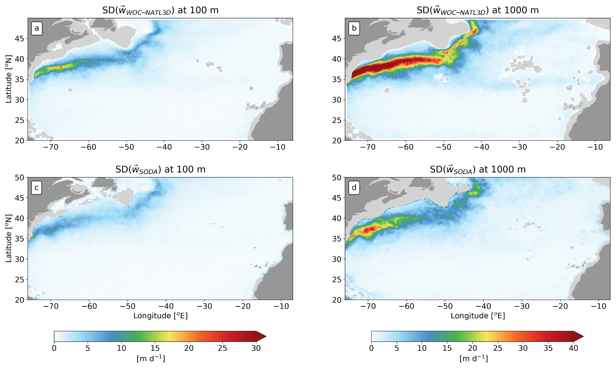
Figure 1 Vertical velocity standard deviation (m d⁻¹) for WOC-NATL3D (a, b) and SODA (c, d) at 100 m (a, c) and 1000 m (b, d). The standard deviation is computed over the period 2010–2016.

2.3.2 3D current retrieval

WOC-NATL3D vertical velocity fields were obtained by solving the quasi-geostrophic omega equation's diabatic Q vector formulation (Giordani et al., 2006; Buongiorno Nardelli et al., 2018):

$$\begin{array}{}\text{(1)}& {\mathrm{\nabla }}_h^{\mathrm{2}}\left(N^{\mathrm{2}}w\right)+f^{\mathrm{2}}{\displaystyle \frac{{\partial }^{\mathrm{2}}w}{\partial z^{\mathrm{2}}}}={\mathrm{\nabla }}_h.\mathit{Q},\end{array}$$

with w being the vertical velocity, N² the Brunt–Väisälä frequency, f the Coriolis parameter and h the horizontal components. The Q vector is made up of three components defining different processes, described in the set of Eq. (2) below:

$$\begin{array}{}\text{(2)}& \begin{array}{rl}& \mathit{Q}=\mathrm{2}{\mathit{Q}}_{\mathrm{twg}}+{\mathit{Q}}_{\mathrm{th}}+{\mathit{Q}}_{\mathrm{dm}}\\ & {\mathit{Q}}_{\mathrm{twg}}={\displaystyle \frac{g}{{\mathit{\rho }}_{\mathrm{0}}}}\left({\displaystyle \frac{\partial u_g}{\partial x}}{\displaystyle \frac{\partial \mathit{\rho }}{\partial x}}+{\displaystyle \frac{\partial v_g}{\partial x}}{\displaystyle \frac{\partial \mathit{\rho }}{\partial y}},{\displaystyle \frac{\partial u_g}{\partial y}}{\displaystyle \frac{\partial \mathit{\rho }}{\partial x}}+{\displaystyle \frac{\partial v_g}{\partial y}}{\displaystyle \frac{\partial \mathit{\rho }}{\partial y}}\right)\\ & {\mathit{Q}}_{\mathrm{dm}}={\displaystyle \frac{f}{{\mathit{\rho }}_{\mathrm{0}}}}\left({\displaystyle \frac{{\partial }^{\mathrm{2}}}{\partial z^{\mathrm{2}}}}\left[\mathit{\rho }{K}_m\left({\displaystyle \frac{\partial v_g}{\partial z}}+{\displaystyle \frac{\partial v_{\mathrm{Ekman}}}{\partial z}}\right)\right],\right.\\ & \left.-{\displaystyle \frac{{\partial }^{\mathrm{2}}}{\partial z^{\mathrm{2}}}}\left[\mathit{\rho }{K}_m\left({\displaystyle \frac{\partial u_g}{\partial z}}+{\displaystyle \frac{\partial u_{\mathrm{Ekman}}}{\partial z}}\right)\right]\right)\\ & {\mathit{Q}}_{\mathrm{th}}={\mathrm{\nabla }}_h\left({\displaystyle \frac{\partial }{\partial z}}\left[K_{\mathit{\rho }}\left(N^{\mathrm{2}}+{\displaystyle \frac{g}{{\mathit{\rho }}_{\mathrm{0}}}}{\mathit{\gamma }}_{\mathit{\rho }}\right)\right]\right),\end{array}\end{array}$$

where twg, dm and th represent the kinematic deformation, the turbulent momentum and the turbulent buoyancy components respectively; ρ is the potential density; g is the gravitational acceleration; and (u_g,v_g) and (u_Ekman,v_Ekman) represent the geostrophic and Ekman horizontal velocities. The terms K_m and K_ρ denote the turbulent viscosity and diffusivity, and γ_ρ is a non-local tracer effective gradient. These terms are computed in the OMEGA3D processing through the K-profile parameterization, with the method described in Smyth et al. (2002), which was only modified by Buongiorno Nardelli (2020b) to handle non-staggered non-uniform vertical grids.

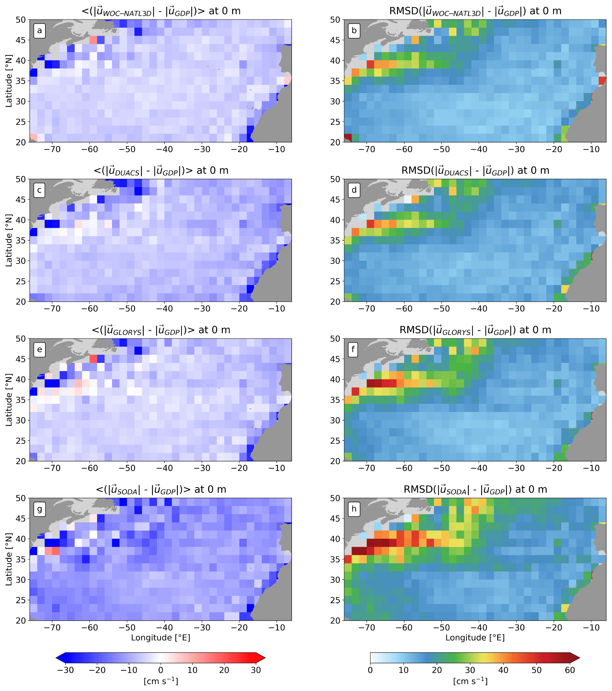
Figure 2 Mean biases (left panels) and RMSDs (right panels) between GDP drifters and WOC-NATL3D (a, b), DUACS (c, d), GLORYS (e, f) and SODA (g, h) surface currents in 2°×2° bins, computed over the period 2010–2016.

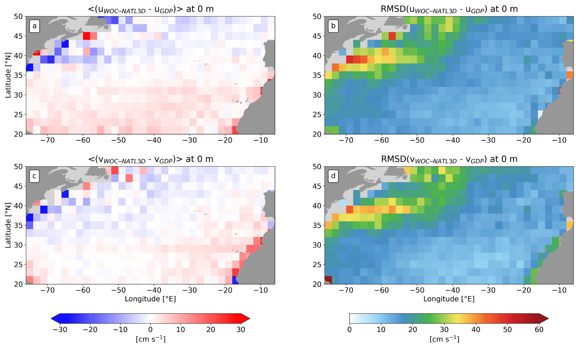
Figure 3 Mean biases (a, c) and RMSDs (b, d) between GDP drifters and the WOC-NATL3D zonal component u (a, b) and meridional component v (c, d) of surface currents. Statistics are computed in 2°×2° bins, over the period 2010–2016.

Figure 4 Panel (a) is the difference between WOC-NATL3D RMSD (Fig. 2b) and DUACS RMSD (Fig. 2c), and panel (b) is the difference between WOC-NATL3D RMSD (Fig. 2b) and GLORYS (Fig. 2d). They are computed at the surface over the period 2010–2016. The RMSDs are computed from GDP drifter velocities.

In order to further improve the product performances at the surface level, we removed the non-local flux of momentum from the formulation of the upper- layer mixing parameterization, and we further constrained the viscosity values not to exceed a consistent empirical estimate and included an empirical estimation of the Ekman shear based on the Copernicus product described in Sect. 2.1.3. Specifically, in order to introduce some more realistic ageostrophic shear in the Ekman layer, we assumed that the background Ekman velocity can be approximated through an analytical fit of the ageostrophic currents (provided at 0 and 15 m by Copernicus Ekman empirical reconstruction, product ID: MULTIOBS_GLO_PHY_REP_015_004) to a compressed Ekman spiral:

$$\begin{array}{l}{\displaystyle }{u}_{\mathrm{Ekman}}\left(z\right)=e^{\frac{z}{D_{\mathrm{amp}}}}\left[u_{\mathrm{0}}\cos \left({\displaystyle \frac{z}{D_{\mathrm{rot}}}}\right)-v_{\mathrm{0}}\sin \left({\displaystyle \frac{z}{D_{\mathrm{rot}}}}\right)\right]\\ {\displaystyle }{v}_{\mathrm{Ekman}}\left(z\right)=e^{\frac{z}{D_{\mathrm{amp}}}}\left[u_{\mathrm{0}}\sin \left({\displaystyle \frac{z}{D_{\mathrm{rot}}}}\right)+v_{\mathrm{0}}\cos \left({\displaystyle \frac{z}{D_{\mathrm{rot}}}}\right)\right],\end{array}$$

where u₀ and v₀ are the components of the empirical Ekman current at 0 m, the depth z is taken as positive upward, and D_amp and D_rot represent the Ekman depth estimates obtained from the amplitude decay and the vector rotation between 0 and 15 m depth respectively (see Roach et al., 2015).

In addition, the viscosity in the Ekman layer, illustrated by K_m in Eq. (2), is also constrained by an analytical profile estimated empirically (defined in Nagai et al., 2006), with a maximum viscosity K_max derived from the local Ekman amplitude decay scale:

$$\begin{array}{}\text{(3)}& K_{\mathrm{empirical}}=K_{max}\left[\mathrm{1}+\tanh \left({\displaystyle \frac{z-D_{\mathrm{amp}}}{\mathit{\delta }}}\right)\right],\end{array}$$

where δ represents the thickness of the transition layer (here set to 40 m, as in Nagai et al., 2006), and $K_{max}=\frac{f{D}_{\mathrm{amp}}^{\mathrm{2}}}{\mathrm{2}}$.

Note that the removal of the nonlocal flux of momentum from the formulation of the upper-layer mixing parameterization and the constraint imposed on the viscosity values allow to correct the dynamically inconsistencies eventually found in the surface layer within the Copernicus Marine Service OMEGA3D product.

The equations are numerically solved by iteratively performing a matrix inversion on a linear system in w. Once vertical velocities are known, they are used to retrieve ageostrophic horizontal velocities. The numerical scheme is exactly the same as the one described in Buongiorno Nardelli (2020b), which was only adapted to the higher-horizontal-resolution grid.

3 Results

3.1 Comparison of vertical velocity to model reanalysis

Measuring vertical velocities in the ocean is challenging mostly because they are extremely small (order of 1–100 m d⁻¹). As there is a very limited number of data available, WOC-NATL3D vertical velocity is compared here to SODA model reanalysis, which provides an estimation of the vertical velocity at a $\mathrm{1}/\mathrm{4}$° resolution. As SODA presents a temporal resolution of 5 d, WOC-NATL3D vertical velocities are averaged every 5 d in order to be consistent.

The standard deviation of vertical velocity computed over 2010–2016 (overlapping period of the 2 products) at 100 and 1000 m for WOC-NATL3D and SODA is displayed in Fig. 1. For both products, the standard deviations of retrieved vertical velocity patterns are very similar. The domain is dominated by the intense activity associated with the Gulf Stream, which shows a strong signature at 1000 m (Fig. 1a, c). Generally, WOC-NATL3D reveals more intense vertical velocities, likely due to a more efficient representation of the small-scale processes.

Figure 5 Mean biases (a, c, e) and RMSD (b, d, f) between GDP drifters and WOC-NATL3D (a, b), DUACS (c, d), GLORYS (e, f) and SODA (g, h) currents at 15 m depth in 2°×2° bins, computed over the period 2010–2016.

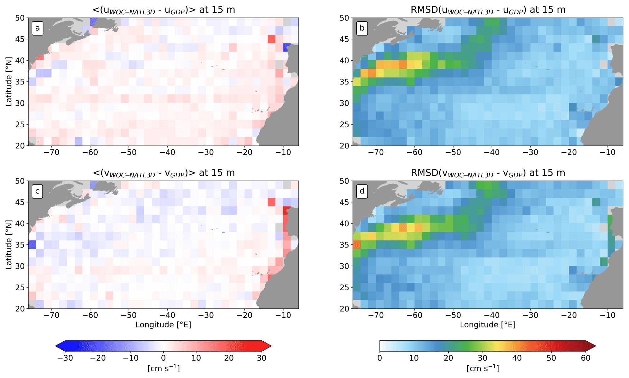
Figure 6 Mean biases (a, c) and RMSDs (b, d) between GDP drifters and the WOC-NATL3D zonal component u (a, b) and meridional component v (c, d) of currents at 15 m. Statistics are computed in 2°×2° bins, over the period 2010–2016.

3.2 Horizontal velocity validation

Horizontal velocities can be inferred from the vertical integration of an equation found during the analytical derivation of Eq. (1) (see Eqs. (3a) and (3b) in Buongiorno Nardelli, 2020b). In this section, the performance of WOC-NATL3D to retrieve horizontal velocities is analyzed and evaluated against DUACS, GLORYS and SODA accuracies. This is obtained by comparing the horizontal currents, at some specific depths, from those products to the data from GDP drifters, in terms of biases and root mean squared differences (RMSDs). First of all, for consistency, WOC-NATL3D and GLORYS horizontal velocities are downgraded from $\mathrm{1}/\mathrm{10}$ and $\mathrm{1}/\mathrm{12}$° respectively to $\mathrm{1}/\mathrm{4}$° horizontal grid and 5 d averaged to match SODA spatial and temporal resolution. DUACS velocities are 5 d averaged as well. The time span is restricted to 2010–2016, corresponding to the overlapping period of all datasets. Then, drifters and datasets are co-located in time (±2 d) and space (to the nearest grid point), and horizontal velocities are vertically interpolated at drifter depths (in this paper, 0, 15 and 1000 m) through a weighted average of the two closest levels (for 15 and 1000 m depths). The matchup maps are shown in Appendix A.

Figure 7 Difference between WOC-NATL3D RMSD (Fig. 5b) and GLORYS RMSD (Fig. 5d) at 15 m depth, over the period 2010–2016. The RMSDs are computed from GDP drifter velocities.

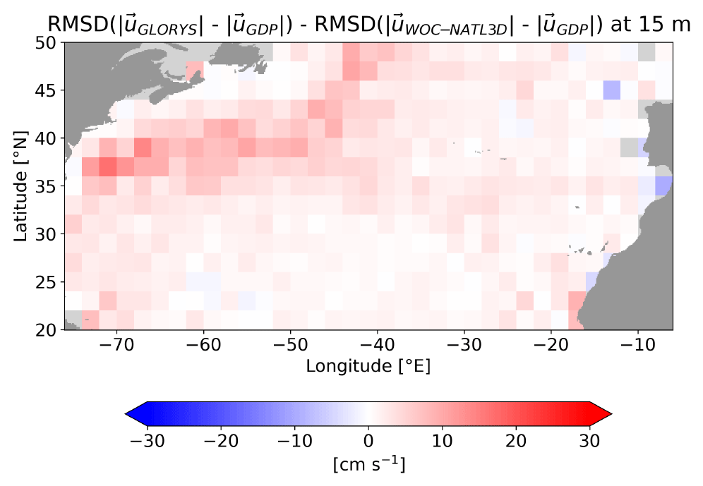
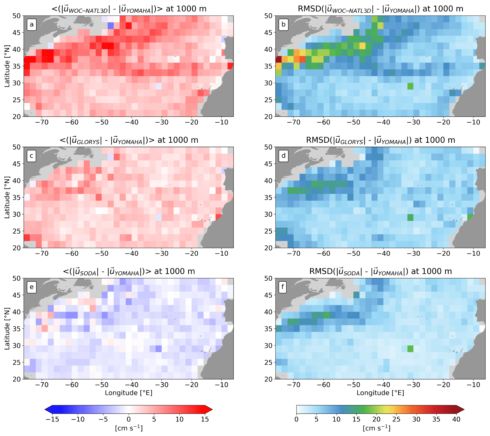
Figure 8 Mean biases (a, c, e) and RMSDs (b, d, f) between YOMAHA drifters and WOC-NATL3D (a, b), GLORYS (c, d) and SODA (e, f) currents at 1000 m in 2°×2° bins, computed over the period 2010–2016.

Mean biases between GDP drifters and WOC-NATL3D, DUACS, GLORYS and SODA total horizontal velocities as well as their associated RMSDs at 0 m, computed in 2°×2° bins, are shown in Fig. 2. All mean biases appear to have a similar pattern, with the largest absolute values localized in the Gulf Stream, the place of intense mesoscale activity, or along the African coast, where a strong upwelling occurs. Those values reveal a general underestimation of the horizontal current intensity in WOC-NATL3D, altimetry and the models (Fig. 2a, c, e, g). While WOC-NATL3D, DUACS and GLORYS show equivalent mean bias values, −5.2, −6.9 and −5.2 cm s⁻¹ respectively, SODA velocities reflect more prominent differences regarding in situ observations, with a mean bias of −11.6 cm s⁻¹. Note that few positive bias values are observed in the Gulf Stream. Regarding the RMSD distribution, all products display the same pattern, with, as expected, the strongest values located in the Gulf Stream. WOC-NATL3D and DUACS RMSD values are very close, showing mean RMSD values of 13.9 and 14.7 cm s⁻¹ respectively. Model reanalyses reflect the highest mean RMSD values, 15.7 cm s⁻¹ for GLORYS and 19.7 cm s⁻¹ for SODA, with some RMSDs reaching up to 57 cm s⁻¹ for GLORYS and 81 cm s⁻¹ for SODA in the Gulf Stream. It should be noted that some spikes in WOC-NATL3D statistics are visible at the Strait of Gibraltar and in the lower left corner of the domain. Some aberrant velocities, likely due to the presence of a coastline, were not flagged during the computation of statistics, resulting in unusually high values of RMSD and bias.

To examine this further, mean bias and mean RMSD statistics are performed separately for the two components (u and v) of the surface current between GDP drifters and WOC-NATL3D, as depicted in Fig. 3. The mean biases of WOC-NATL3D reveal distinct characteristics within the domain. Above 35° N, the model underestimates the zonal component of the surface current, while south of this latitude, it overestimates it (Fig. 3a). The bias distribution of the meridional velocity exhibits a slightly different pattern, characterized by underestimation concentrated more in the northwest part of the domain (Fig. 3c). Notably, a significant overestimation of this component is observed along the African coast. In both components, high biases are observed in the Gulf Stream. The RMSDs, depicted in Fig. 3b and c, closely match the total velocity RMSDs presented in Fig. 2b. It is noteworthy that WOC-NATL3D represents the zonal current more effectively than the meridional current, supported by RMSD mean values of 17 cm s⁻¹ for the zonal component and 16.6 cm s⁻¹ for the meridional one.

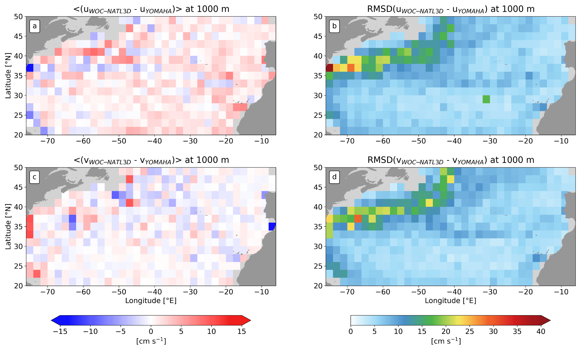
Figure 9 Mean biases (a, c) and RMSDs (b, d) between GDP drifters and the WOC-NATL3D zonal component u (a, b) and meridional component v (c, d) of currents at 1000 m. Statistics are computed in 2°×2° bins, over the period 2010–2016.

Figure 10 Difference between WOC-NATL3D RMSD (Fig. 8b) and GLORYS RMSD (Fig. 8d) at 1000 m depth, over the period 2010–2016. The RMSDs are computed from YOMAHA drifter velocities.

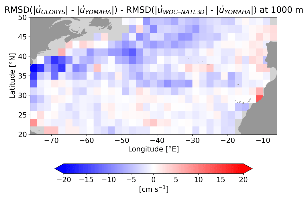
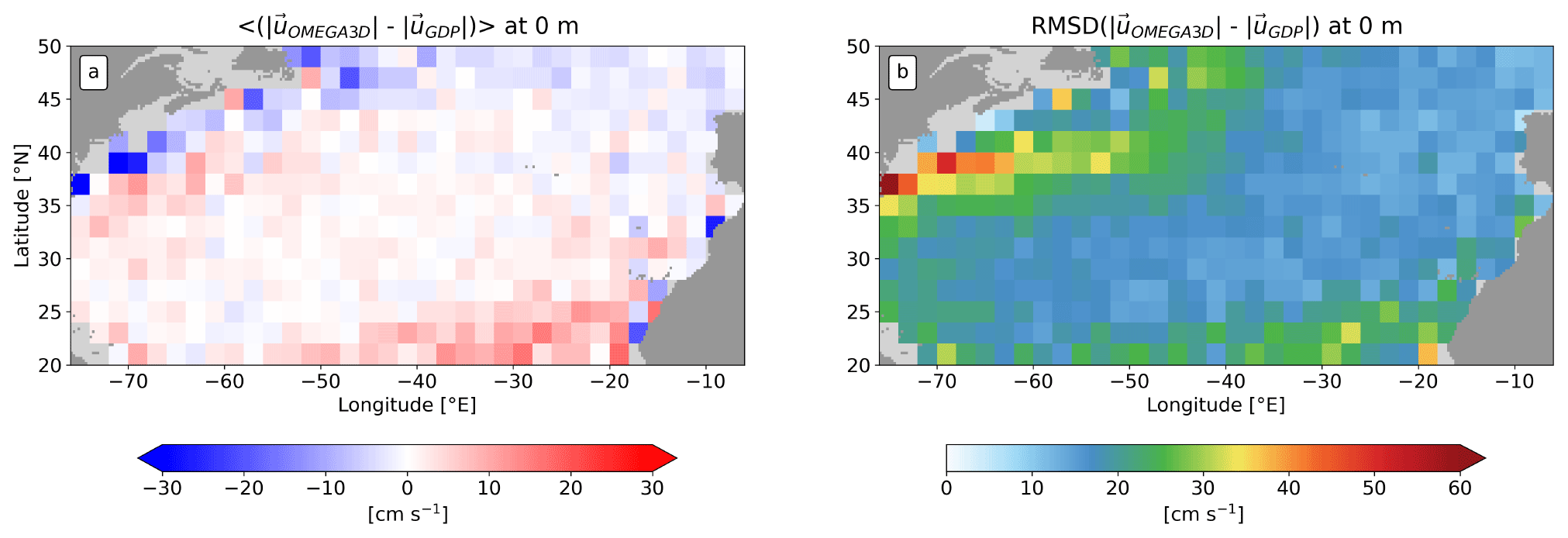
Figure 11 Mean bias (a) and RMSD (b) between GDP drifters and OMEGA3D surface currents in 2°×2° bins, computed over the period 2010–2016.

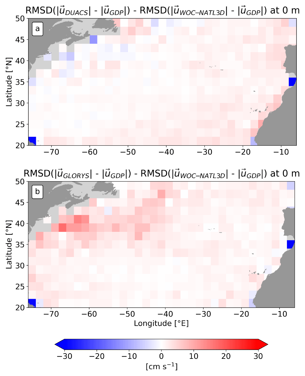
To highlight the discrepancies discussed above about total horizontal velocities, differences between GLORYS RMSDs, DUACS RMSDs and WOC-NATL3D RMSDs are presented in Fig. 4. A clear improvement of WOC-NATL3D velocities is observed, reflected by positive values, with respect to GLORYS, especially along the Gulf Stream (Fig. 4b). In the top panel of Fig. 4, even though the improvement is not as strong, WOC-NATL3D reveals slight progress compared to the simple geostrophic estimates from satellites and confirms the lower mean RMSD of WOC-NATL3D.

Biases and RMSDs are also computed at 15 m depth between the drifters and WOC-NATL3D, GLORYS and SODA (Fig. 5). Once again, WOC-NATL3D and GLORYS patterns look similar. The currents tend to be generally underestimated despite a slight overestimation of GLORYS at some locations in the Gulf Stream. WOC-NATL3D and GLORYS reveal a mean bias of −3.3 and −1.9 cm s⁻¹ respectively, whereas SODA appears more biased, with a mean value of −8.4 cm s⁻¹. Note that the smaller mean bias value observed for GLORYS does not necessarily reflects a better overall behavior than the WOC-NATL3D product. The currents' overestimations seen in GLORYS along the Gulf Stream might compensate for the mean bias value. RMSDs at 15 m shown in Fig. 5b, d and f display an analogous pattern to the one at the surface (see Fig. 2), with the largest values concentrated along the Gulf Stream. As before, statistics are computed for the two components of the currents at 15 m, specifically for the WOC-NATL3D product, and are presented in Fig. 6. Even though the v component seems to still display more negative biases in the north part of the domain, mean bias values of the zonal velocity no longer exhibit a clear pattern as observed at the surface. The zonal component displays a mean bias of 0.95 cm s⁻¹ (Fig. 6a), while the meridional component shows a negative mean bias of 0.43 cm s⁻¹ (Fig. 6c). RMSDs, illustrated in Fig. 6b and d, are highly similar for both components, with a value of 15 cm s⁻¹ for the zonal velocity and 15.2 cm s⁻¹ for the meridional velocity, aligning closely with the total horizontal velocity (Fig. 5b).

GLORYS RMSD and WOC-NATL3D RMSD values of the total horizontal current are also compared, and the result is illustrated in Fig. 7. This figure highlights the higher RMSD values of GLORYS compared to WOC-NATL3D, with respect to drifters. The positive values show a clear improvement of WOC-NATL3D velocities over modeled velocities, especially along the Gulf Stream.

The same analysis is repeated at 1000 m depth. WOC-NATL3D, GLORYS and SODA deep total horizontal currents are compared to the YOMAHA observation dataset, providing horizontal currents at 1000 m depth. First of all, Fig. 8a and c bring out a general overestimation of the currents by WOC-NATL3D and GLORYS. WOC-NATL3D occurs to be more biased than GLORYS, with a mean bias of 4.9 cm s⁻¹ against 2.9 cm s⁻¹ for GLORYS. The strongest WOC-NATL3D biases are observed, once again, in the Gulf Stream but also along the Azores current (35° N), reaching a maximum of 43 cm s⁻¹, while GLORYS bias values do not exceed 12 cm s⁻¹. Conversely, SODA seems to rather underestimate velocities, with sparse positive biases mainly located along the Gulf Stream (Fig. 8e) and with a negative mean bias of 1.3 cm s⁻¹, substantially lower than the other products. Regarding RMSDs (Fig. 8b, d and f), the largest values are clearly found along the Gulf Stream, with WOC-NATL3D displaying the highest values (mean RMSD of 9.8 cm s⁻¹) of all. As seen in Fig. 8a, slightly strongest WOC-NATL3D RMSDs along the latitude 35° N highlight the presence of the Azores current (Fig. 8b). In addition, Fig. 9 illustrates mean biases and mean RMSDs for the two components of the velocity between WOC-NATL3D and YOMAHA. WOC-NATL3D shows a tendency to overestimate the zonal current more than the meridional one (Fig. 9a and c) across the domain, with mean bias values of 0.94 and −0.05 cm s⁻¹ respectively. As for RMSDs, the patterns are very similar, displaying mean values of 7.7 and 7.9 cm s⁻¹ for the zonal and meridional components respectively (Fig. 9b and d). The distribution of RMSDs for both components also corresponds to that of the total velocity RMSDs, presented in Fig. 8b.

To go further, WOC-NATL3D and GLORYS RMSDs of the total horizontal velocity are specifically compared. Figure 10 reveals a heterogeneous pattern. The area of the Gulf Stream is dominated by negative values, suggesting that GLORYS performs better than WOC-NATL3D at 1000 m. However, some locations seem to show an improvement of WOC-NATL3D deep current.

Additionally, we assessed WOC-NATL3D horizontal velocities against OMEGA3D. In order to avoid redundancy, most of OMEGA3D figures are not shown here, and the reader is invited to refer to Buongiorno Nardelli (2020b), regarding the description and validation of the OMEGA3D currents at 15 and 1000 m depth. Yet, OMEGA3D performance at the surface (0 m) was not assessed in Buongiorno Nardelli (2020b). Therefore, biases and RMSDs between GDP drifters and OMEGA3D horizontal velocities are computed at the surface and shown in Fig. 11. Before comparing with WOC-NATL3D, it is relevant to mention that drifters and OMEGA3D data were co-located considering their concomitant locations at times ±3 d rather than at times ±2 d as performed previously. This is done to account for OMEGA3D temporal resolution of 7 d (matchup map in Appendix A). Unlike WOC-NATL3D (Fig. 2a), OMEGA3D shows contrasted bias values. Overall, bias values are positive, which means that OMEGA3D overestimates surface horizontal velocities, but some negative values are observed along the Gulf Stream, close to the coast and in the northern part of the domain (Fig. 11a). Besides showing the “usual” high values along the Gulf Stream, Fig. 11b also reveals high RMSDs in the south of the domain, between 20 and 25° N, which is not observed in the WOC-NATL3D product (Fig. 2b).

Differences between WOC-NATL3D RMSDs and OMEGA3D RMSDs of the horizontal velocity intensity and of its directional components at the surface are illustrated in Figs. 12 and 13. It reveals essentially positive values, which indicates that WOC-NATL3D horizontal velocities are closer to in situ velocities than OMEGA3D horizontal velocities, both in magnitude and direction. This stresses the enhancement of WOC-NATL3D at solving vertical velocities close to the surface with respect to OMEGA3D.

Figure 12 Difference between WOC-NATL3D RMSD (Fig. 2b) and OMEGA3D RMSD (Fig. 11b) at the surface, over the period 2010–2016. The RMSDs are computed from GDP drifter velocities.

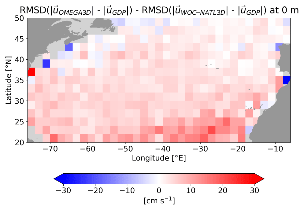
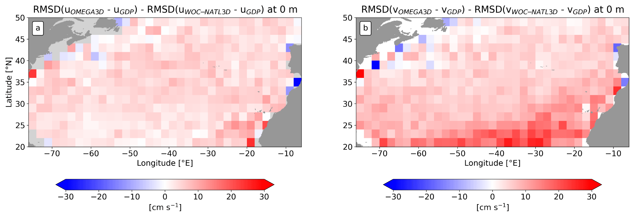
Figure 13 Difference between the WOC-NATL3D RMSD and OMEGA3D RMSD zonal component u (a) and meridional component v (b) at the surface. The RMSDs are computed from GDP drifter velocities, over the period 2010–2016.

3.3 Spectral analysis

In this last section, a spectral analysis of the horizontal velocity field at 15 m is presented in order to highlight more quantitatively the energy distribution. The power spectral density (PSD) of the zonal and meridional velocity components is estimated using Welch's method, based itself on fast Fourier transform (Fig. 14).

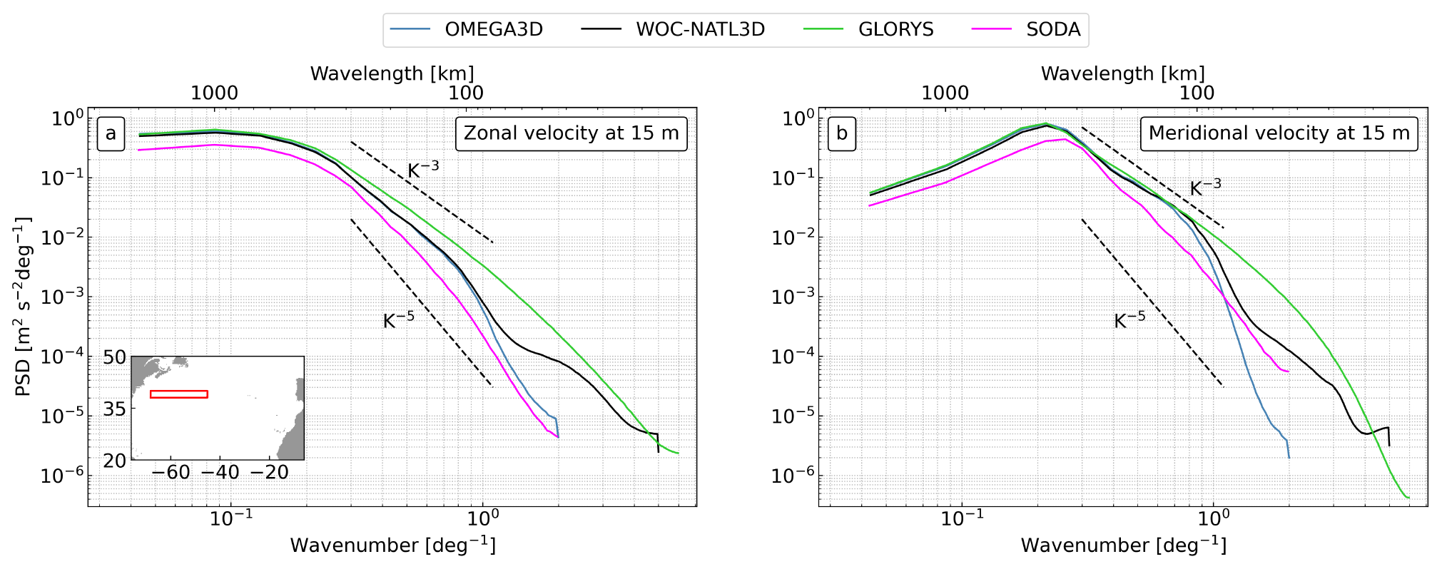
Figure 14 Power spectra density (m² s⁻² per degree) of horizontal velocity at 15 m depth averaged over 2010–2016: zonal component (a) and meridional component (b). The spectra are performed in the box shown in the inset map. Dashed lines indicate slopes of −3 and −5.

The analysis focuses on the Gulf Stream region, a highly energetic region. Wavenumber spectra are computed in the box shown in the insert of Fig. 14a (38–40° N, 45–68° W) along each latitude and then time averaged over 2010–2016 to obtain a single spectrum for every product (GLORYS, SODA, OMEGA3D and WOC-NATL3D). For a better understanding, a second x axis representing wavelengths in kilometers is added on the top of the plots. Slopes of k⁻³ and k⁻⁵ are also indicated by dashed lines.

At low wavenumbers, all zonal velocity PSDs are in agreement, indicating a fairly equivalent representation of the largest mesoscale motion (Fig. 14a). A spectral break occurs at 400–500 km, followed by a drop in energy close to k⁻³ slope for the GLORYS spectrum and k⁻⁵ for the SODA spectrum, which respectively show the highest and lowest variance. WOC-NATL3D and OMEGA3D spectra present an energy reduction, with a slope between k⁻³ and k⁻⁵. Up to approximately 0.7 per degree (122 km), OMEGA3D and WOC-NATL3D spectra lie very close. Beyond this point, OMEGA3D experiences a significant loss in variance, while WOC-NATL3D continues with its pattern before flattening at 4 per degree, its effective resolution (nominal resolution $\mathrm{1}/\mathrm{10}$°).

Meridional velocity spectra are displayed in Fig. 14b. At large scales (<0.8 per degree), spectra are similar and follow a slope of k⁻³, except for SODA, which presents less energy and a steeper slope (k⁻⁵). At 0.2–0.3 per degree, spectra drop off and follow a slope of k⁻³ and k⁻⁵ for SODA. At 0.7–0.8 per degree, WOC-NATL3D and OMEGA3D spectra start to decrease rapidly before flattening between 3 and 4 per degree for the former and abruptly dropping off at 2 per degree for the latter. These two values represent WOC-NATL3D and OMEGA3D effective resolutions. In other words, even though WOC-NATL3D nominal resolution is $\mathrm{1}/\mathrm{10}$°, it does not fully resolve processes at scales $<\mathrm{1}/\mathrm{4}$°. This is probably the consequence of the use of satellite data. In fact, filtering and interpolation are inherent in the construction of L4 SST or SSS and affect the final product. Note that the OMEGA3D meridional velocity spectrum becomes even less energetic than the SODA spectrum around 90 km.

4 Data availability

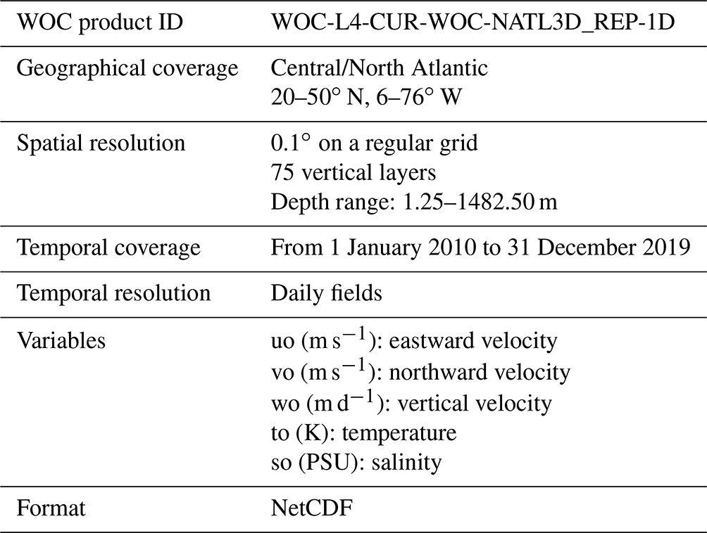
The WOC-NATL3D is freely available on the World Ocean Circulation website at https://doi.org/10.12770/0aa7daac-43e6-42f3-9f95-ef7da46bc702 (Buongiorno Nardelli, 2022). The characteristics of the product are summarized in Table 1.

Table 1 Description of the product.

5 Conclusions

In the framework of the ESA-WOC project Theme 2 “Sustainable fisheries”, a new product, WOC-NATL3D, has been developed to provide a high-resolution reconstruction of ocean 3D dynamics in the North Atlantic. The WOC-NATL3D product is based on the omega diagnostic tool originally used in the framework of the European Copernicus Marine Service to deliver a global product of 3D ocean currents that includes the vertical component of the velocity (OMEGA3D, Buongiorno Nardelli, 2020b). The OMEGA3D product was built using a method based on the quasi-geostrophic omega equation, and its horizontal velocities generally display higher accuracy than velocities provided by model reanalyses when compared to independent drifter observations. However, the OMEGA3D product is more suited for studies of the global dynamics and associated interannual variability than for applications targeting an accurate assessment of mesoscale-driven dispersion and transport, such as those required by the ESA-WOC project. To build this new product and improve its accuracy in the layers close to the surface, we have thus adapted the omega diagnostic tool to a high-resolution grid and implemented some modifications in the formulation of the Q vector initially used by Buongiorno Nardelli (2020b). These especially concern the component defining the turbulent momentum. By taking advantage of the modeled horizontal Ekman currents provided by Copernicus at two different depths, a background empirical ageostrophic shear term is introduced. It is assumed that the background Ekman velocity can be approximated through an analytical fit of the ageostrophic currents to a compressed Ekman spiral. The viscosity within the Ekman layer is also empirically constrained to reduce the differences between the background and retrieved horizontal ageostrophic velocities. Furthermore, potential density and geostrophic currents, used to compute the forcing terms due to the flow deformation in the omega equation, are reconstructed using a stacked Long Short-Term Memory neural network that projects sea surface satellite data at depth after training with sparse co-located in situ vertical profiles (Buongiorno Nardelli, 2020a).

The WOC-NATL3D vertical velocity was compared to the model reanalysis SODA, one of the rare products that also provide vertical velocities. WOC-NATL3D shows more intense values and, due to its higher effective spatial resolution, is able to capture small-scale dynamics. Total horizontal velocities, inferred from the vertical velocities, were assessed through an inter-comparison with model reanalyses and altimeter data, based on the statistics of the differences computed against drifter data. As with the other products close to the surface, WOC-NATL3D generally underestimates the total horizontal velocities compared to GDP drifters. Both WOC-NATL3D and GLORYS display a lower bias compared to satellite or SODA, with WOC-NATL3D achieving the lowest RMSD values. At 15 m, the systematic error in WOC-NATL3D, estimated with respect to GDP, is only slightly higher than in GLORYS. At 1000 m, taking YOMAHA drifter velocity estimates as reference, WOC-NATL3D reflects the highest biases and RMSD values, and a direct comparison between WOC-NATL3D RMSDs and GLORYS RMSDs highlights a deterioration of the horizontal currents in WOC-NATL3D. Additionally, individual components of horizontal velocity were examined, focusing specifically on WOC-NATL3D in comparison to drifter datasets. At the surface, WOC-NATL3D tends to underestimate the zonal component above 35° latitude and overestimates the meridional component in the northwest part of the domain. In the rest of the domain, it underestimates both components. At 15 m depth, the meridional biases remain predominantly negative in the northern part of the domain, while the zonal biases no longer exhibit the north–south pattern observed at the surface. Deeper, at 1000 m, WOC-NATL3D tends to generally overestimate u more than v. Regarding WOC-NATL3D RMSDs at all depths, they mirror the RMSD values of the total horizontal intensity both in terms of values and pattern, with the highest values localized in the Gulf Stream.

Comparing WOC-NATL3D to OMEGA3D directly confirms an improved performance of the new empirical parameterization in the upper layer, both in magnitude and direction. Spectral analysis evidences that WOC-NATL3D presents energy at small scales, more than SODA or OMEGA3D.

WOC-NATL3D behaves well, but there are still some caveats to this data-driven approach. As for OMEGA3D, WOC-NATL3D is not designed for studying coastal dynamics (due to Dirichlet conditions imposed at topographical boundaries; see Buongiorno Nardelli, 2020b). Despite this potential limitation, WOC-NATL3D has demonstrated a good performance in the upper layer of the ocean with horizontal velocities and so of vertical velocities. To conclude, this work aims to contribute to studies of the North Atlantic region by offering a new gridded product of the data-driven 3D reconstruction of ocean currents at high resolution.

Appendix A: Matchup database

In order to built the matchup database, drifters (GDP and YOMAHA) and datasets (WOC-NATL3D, DUACS, GLORYS, SODA) are co-located in space and time. First, only drifter data with a date common to all datasets (according to the chosen depth) are kept. Then, data are spatially co-located by simply finding the closest grid point in the products. Horizontal velocities are vertically interpolated at drifter depths through a weighted average of the two closest levels. Figure A1 illustrates the number of matchups between WOC-NATL3D, DUACS, GLORYS, SODA and GDP drifters at 0 and 15 m (note that DUACS data are not considered in the matchup at 15 m), and Fig. A2 shows the number of matchups between WOC-NATL3D, GLORYS, SODA and YOMAHA drifters at 1000 m. In this paper, 41 820 drifters at the surface, 35 443 at 15 m and 2036 at 1000 m are used to performed the analyses over the period 2010–2016.

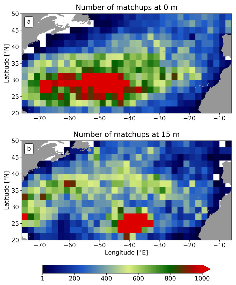
Figure A1 Number of matchups between WOC-NATL3D, DUACS, GLORYS, SODA and GDP drifters at 0 m (a) and between WOC-NATL3D, GLORYS, SODA and GDP drifters at 15 m (b). These matchup numbers are computed over the period 2010–2016 and within 2°×2° bins.

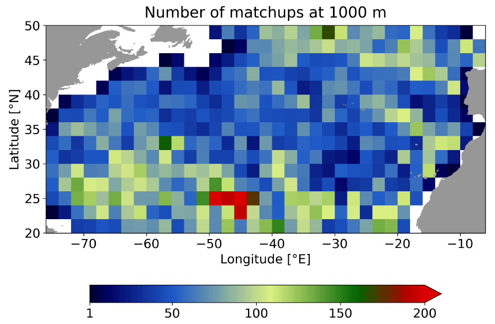
Figure A2 Number of matchups between WOC-NATL3D, GLORYS, SODA and YOMAHA drifters at 1000 m, computed over the period 2010–2016 and within 2°×2° bins.

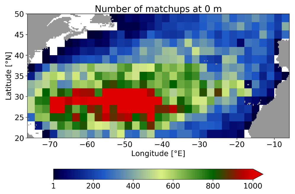
Figure A3 Number of matchups between WOC-NATL3D, OMEGA3D and GDP drifters at 0 m, computed over the period 2010–2016 and within 2°×2° bins.