Extension of a high temporal resolution sea level time series at Socoa (Saint-Jean-de-Luz, France) back to 1875

In this data paper, the sea level time series at Socoa (Saint-Jean-de-Luz, southwestern France) is extended through a data archaeology exercise. We conducted a comprehensive study of national and local archives to catalogue water level records stored in ledgers (handwritten record books) and charts (marigrams from mechanical float gauges), along with other associated documents (metadata). A dedicated effort was undertaken to preserve more than 2000 documents by archiving them in digital formats. Using this large set of rescued documents, the Socoa time series has been extended back to 1875, with more than 58 station-years of additional data. The final time series has hourly sampling, while the raw dataset has a finer sampling frequency of up to 5 min. By analysing precise levelling information, we assessed the continuity of the vertical datum. We also compared the new century-long time series to nearby tide gauge data to ensure its datum consistency. While the overall quality of the time series is generally good, siltation of the stilling well has occasionally affected certain parts of the record. We have successfully identified these impacted periods and flagged the corresponding data as doubtful. This extended high-resolution sea level time series at Socoa, spanning more than 100 years, will be valuable for advancing climate research, particularly when studying the decadal-scale variations in the North Atlantic and investigating the storminess and extreme events along the French Basque coast. The raw digitized water level, the processed dataset, metadata, and the python notebooks used for processing are available at https://doi.org/10.5281/zenodo.7438469 (Khan et al., 2022).

1 Introduction

Tide gauge records are among the oldest instrumental datasets. They have a crucial role in our understanding of contemporary sea level variability and climate change (Ekman, 1999; Church et al., 2013). Between 1901 and 2010, the global mean sea level (GMSL) has been rising at a rate of 1.5±0.4 mm yr⁻¹ (Oppenheimer et al., 2019). The assessment of the sea level rise during the 19th and 20th centuries (which provides a baseline for assessing the changes in the 21st century) relies on long-term tide gauge records (e.g. Dangendorf et al., 2017). A subset of these long time series has become accessible to the scientific community through the process of discovery, digitization, and reconstruction, a procedure which is known as sea level data archaeology (Woodworth, 1999; UNESCO/IOC, 2020).

Over the last few decades, data archaeology has been applied to different parts of the globe to construct and study long-term sea level variability and change (e.g. Woodworth, 1999; Hunter et al., 2003; Woodworth et al., 2010a; Talke et al., 2018). For instance, Woodworth (1999) recovered and analysed the mean high-water levels recorded at Liverpool starting from 1768. Similarly, Wöppelmann et al. (2006a) applied data archaeology to reconstruct a sea level series at Brest back to the beginning of the 18th century. Both studies concluded a similar result – a rising trend from the beginning of the 20th century with an acceleration towards the second half (Wöppelmann et al., 2008). In the Southern Hemisphere, where the data coverage is generally sparse, Testut et al. (2010) recovered water level measurements recorded in 1874 on Saint Paul Island in the southern Indian Ocean. Combined with recent measurements, they revealed a statistically zero relative sea level trend. Similarly, Hunter et al. (2003) recovered and analysed intermittent sea level records made in Port Arthur, Tasmania (southern Australia). They reported an average sea level trend of 0.8±0.2 mm yr⁻¹ relative to land and 1.0±0.3 mm yr⁻¹ considering vertical land motion over the period from 1841 to 2002. At the local scale, some data archaeology studies combine multiple nearby historical tide gauge records into one long time series for sea level trend analysis (Marcos et al., 2011, 2021; Woodworth, 1999), whereas, regionally, Hogarth et al. (2020) combined data archaeology, numerical modelling, and statistical minimization approaches to further extend the mean sea level record for the British Isles. They estimated a robust regional mean sea level trend of 2.39±0.27 mm yr⁻¹ over the period from 1958 to 2018, with an acceleration of 0.058±0.030 mm yr⁻².

Alongside the mean sea level, the tide has also been found to manifest a long-term evolution, and high-frequency (typically hourly or less) data are needed to investigate such changes (Woodworth, 2010; Haigh et al., 2020). During the first half of the 19th century, automatic mechanical tide gauges started to appear, paving the way for systematic, continuous, high-frequency measurements of water levels (Wöppelmann et al., 2006b). By using high-frequency long-term sea level records extended through data archaeology, Pouvreau et al. (2006) analysed the secular trend in the evolution of M2 (the main lunar semidiurnal tide) at Brest. They reported no significant trend but long-period oscillations with a period of 141 years. Recent research on the tidal change shows that the long-term changes are not linear (Ray and Talke, 2019). Pan and Lv (2021) reported a quasi-60-year oscillation in the global tide from a global set of long high-resolution sea level time series. These non-linear changes sometimes show break points around the late 19th century (Pineau-Guillou et al., 2021). These recent results further highlight the necessity of long high-frequency sea level time series for studying the evolution of the tide.

Past high-frequency tide gauge time series are also very useful for the analysis of the extreme sea level (ESL), which is a major societal concern due to the ongoing sea level rise (Oppenheimer et al., 2019). Dedicated studies have been conducted to understand the dynamics and the drivers of the ESL at local (Letetrel et al., 2010; Talke et al., 2014, 2018), regional (Wahl and Chambers, 2015; Marcos et al., 2015; Marcos and Woodworth, 2017), and global (Menéndez and Woodworth 2010) scales. Among various factors, sea level rise is shown to be the first-order driver of the observed ESL change along most of the coastline (Menéndez and Woodworth, 2010) and is projected to be the major factor in future ESL changes globally (Muis et al., 2016, Fox-Kemper et al., 2021). However, ESL variability also varies regionally, depending on the local and regional processes (Menéndez and Woodworth, 2010). Long high-resolution sea-level time series are particularly interesting for unravelling the contributions from the mean sea level change (Letetrel et al., 2010), seasonal and decadal variability (Menéndez and Woodworth 2010; Marcos et al., 2015), and local changes (Talke et al., 2014, 2018). Indeed, it has been concluded with high confidence (meaning high agreement and robust evidence in the available literature) that it is essential to consider localized storm surge processes when monitoring the trend in the ESL (Oppenheimer et al., 2019). Such monitoring requires reliable long high-resolution observations. A long time series provides an additional benefit by reducing the uncertainty of ESL analysis (Coles, 2001), which equates to better flood risk assessment.

Global high-resolution datasets like GESLA (Global Extreme Sea Level Analysis; Woodworth, 2016; Haigh et al., 2022) have been important for current global-scale as well as regional-scale studies on the ESL. Such datasets have also allowed global and regional analyses of the tide (Piccioni et al., 2019) and the non-linearity of the tide–surge interaction (Arns et al., 2020) as well as data driven modelling of surges (Tadesse et al., 2020). Yet, most of the stations in GESLA have time series shorter than 50 years. As demonstrated by previous studies (Wöppelmann et al., 2014; Talke et al., 2014, 2018; Talke and Jay, 2017), data archaeology offers a solution to this scarcity of long-term data by tapping into the potential of rescuing numerous instrumental records worldwide (Bradshaw et al., 2015).

As a response to this lack of long-term high temporal resolution records for the assessment of short- to long-timescale processes, this article presents a data rescue and archaeology effort to make available a high temporal resolution long-term sea level time series at Socoa. The tide gauge is located in Saint-Jean-de-Luz, France, along the Basque coast in the Bay of Biscay (Fig. 1a, b). The region is dominated by strong tides (meso-tidal) and energetic waves (Dodet et al., 2019), making it an important observation location. The tide gauge station at Socoa was established in 1875. However, the earliest available data in the French reference repository before this work (e.g. https://data.shom.fr/donnees/refmar/95, last access: 10 April 2022) starts from 1942, with continuous recording only available from 1964 on (Arnoux et al., 2021). Data are available from hourly sampling before 2011, whereas both high-frequency (1 min) and hourly data are available for 2011 on.

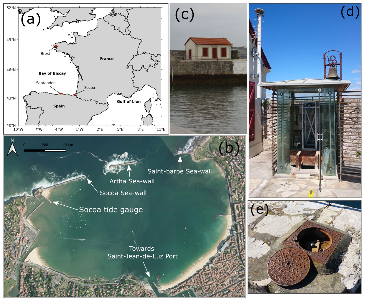
Figure 1 (a) The study area, with the locations of the Socoa tide gauge and other tide gauges used in this study indicated. (b) Satellite view of the study area (source: IGN geoservices, https://geoservices.ign.fr/, last access: 26 January 2022). (c) A view of the tide gauge's surroundings and the housing location. (d) The tide gauge housing over the top of the stilling well. (e) The nearby tide gauge benchmark IGN O.A.K3L3-5-IV. The photos in panels (c), (d), and (e) were provided by SONEL (https://www.sonel.org/, last access: 26 January 2022).

The new extended sea-level time series developed in this work is shown in Fig. 2a, with the existing data shown in grey and the new data shown in black. To describe the development of this new time series, the history of the Socoa tide gauge is first presented in Sect. 2 by considering various instrumentation periods. A summary of the rescued documents (containing data and metadata) is also presented. The rescue process and the analysis of the time series are described in Sect. 3, which is followed by quality control and data quality assessment in Sect. 4. In Sect. 5, we present a trend analysis. The data availability is detailed in Sect. 6, with concluding remarks provided in Sect. 7.

2 History of the Socoa tide gauge station and rescued documents

The Socoa tide gauge station was established during the 1873–1875 period. A dedicated housing (Fig. 1c) with an adjacent stilling-well system (Fig. 1d) was built to host the original tide gauge, to handle the daily tasks of the gauge keeper, as well as to store the paper charts. Several water-level instruments were operated during various periods covering the 19th and 20th centuries, with modern technology used in the 21st century, which is still operating (Fig. 1 in Martín Míguez et al., 2008). In the following sub-sections, we provide descriptions of each instrumentation period, along with detailed information about the catalogued documents.

2.1 The Chazallon tide gauge period: 1875 to 1920

During the 1840s, several float-type tide gauges devised by Antoine M. R. Chazallon (1802–1872) were installed along the French coast. A schematic of such a tide gauge is shown in Fig. 2c. Like most float gauges, the displacement of the float is reduced through a mechanical system, and the resulting sea level variation is recorded on a paper chart controlled by a clock (IOC, 1985). One of the Chazallon-type tide gauges was installed in La Rochelle (Vieux Port) and operated from 1863 to 1874 (Gouriou et al., 2013). This tide gauge was then transferred to Socoa in 1875. At Socoa, the float of the tide gauge was installed in a stilling well located near the housing (Fig. 1d). The Chazallon tide gauge was operational until 1920, when most tide gauges around the French coast were discontinued. Up until then, the tide gauge was operated by the Service Hydrographique de la Marine (SHM), the predecessor of the current Service hydrographique et océanographique de la marine (Shom, https://www.shom.fr/, last access: 26 January 2022).

Two types of historical records have been found for the Chazallon period – (1) a subset of charts and (2) ledgers. The ledgers are 32×49 cm paper documents with water level values obtained by the inspection of the charts by an operator. The ledgers (Fig. S1 in the Supplement) and charts are currently stored at the Shom archive located in Brest (France).

2.2 Temporary tide gauge during the World War II period from 1942 to 1944

In the currently available archives, e.g. Shom or the Permanent Service for Mean Sea Level (PSMSL, Holgate et al., 2013), there are data available for the World War II (WWII) period from November 1942 to May 1944. In fact, 44 charts covering this period were found in the Shom archive at Brest, but the rescued metadata information (discussed in Sect. 2.5) does not include any mention of a tide gauge operating at Socoa. After inspection, we found that these charts had a different paper size compared to those for the Chazallon or Brillie eras, which indicates that it was a different type of tide gauge. In addition, the paper charts bear German markings. Local historians confirm that there was indeed another tide gauge, installed by the Germans, on the other side of the bay in Socoa. The data obtained during WWII appear to be consistent with the rest of the record, as confirmed by a tidal analysis.

2.3 The Brillie tide gauge period: 1950 to 2004

During 1950, a Brillie type float gauge (large model type; Roubertou, 1955) was installed (Fig. 2d) in the stilling well built for the Chazallon gauge. Each chart for this large model type is 72×50 cm in dimension (x–y). The x axis of the paper is divided into 24 divisions (corresponding to each hour), and each hourly division is further subdivided into 10 min subdivisions. On the y axis there is a 1/10 reduction in the water level variation, i.e. the y axis represents a range of 5 m in sea level (50 cm × 10). There are further subdivisions of 25 and 5 cm on the charts. Surprisingly, no documentation was found in the catalogued archives regarding the installation and operation of this tide gauge except for the knowledge of the physical existence of the tide gauge itself till 2004.

The recording of water levels by the Service Maritime des Ponts et Chaussées started in December 1950. In total, 2477 charts spanning the period from December 1950 to 2001 were recovered from the local archive – Archives des Pyrénées-Atlantiques at Bayonne. No data were found for 2002–2003.

The water level curves on the charts during the Brillie period were recorded in the legal time of France (see Sect. 3.2 for further details). Each curve in the charts represents 1 day of the water level record, and each chart was found to contain multiple days of records (Fig. S1c). Typically, up to 14 d of sea levels were recorded on these paper charts. In most cases, the charts were accompanied by a check sheet, which are an important part of the data rescue. See Fig. 2b for the availability of the charts and check sheets.

2.4 The modern instrumentation: from 2004 on

With the advent of the modern RONIM (Réseau d'Observation du Niveau des Mers) sea level measurement network (Martín Míguez et al., 2008), the Brillie tide gauge at Socoa was decommissioned and replaced with a digital radar gauge in 2004 (Fig. 2e). This radar gauge is currently co-located with a continuously operating geodetic global navigation satellite system (GNSS) station (https://www.sonel.org/spip.php?page=gps&idStation=835, last access: 10 April 2022). The antenna of the GNSS station is visible in Fig. 1d. This tide gauge is currently maintained by Shom. Its sea level data and metadata are available at the Shom data portal (https://data.shom.fr, last access: 10 April 2022) in both raw and post-processed quality-controlled forms. Raw data are sampled at 1 min intervals. Data from the tide gauge are accessible through the Global Telecommunication System (GTS) network, which enables a real-time data flow. This data flow enables real-time monitoring of the gauge, which is achieved, for instance, via the Intergovernmental Oceanographic Commission (IOC) Sea Level Station Monitoring Facility (see http://www.ioc-sealevelmonitoring.org/station.php?code=scoa2, last access: 30 June 2023). Note that the data from the IOC Facility should generally not be used for any scientific application, as its main design and procedures have been designed for monitoring the operational status of the gauges (Aarup et al., 2019).

It is worth noting here that at Socoa, the position of the tide gauge remained the same over its full period of observation from November 1875 until now, through the various instrumentation periods. The modern tide gauge is operating within the same stilling well, hence preserving spatial and environmental continuity with past measurements. There is a caveat to this statement concerning modifications made to the stilling well infrastructure in the early recording period, which we will illustrate later in Sect. 4.3.3.

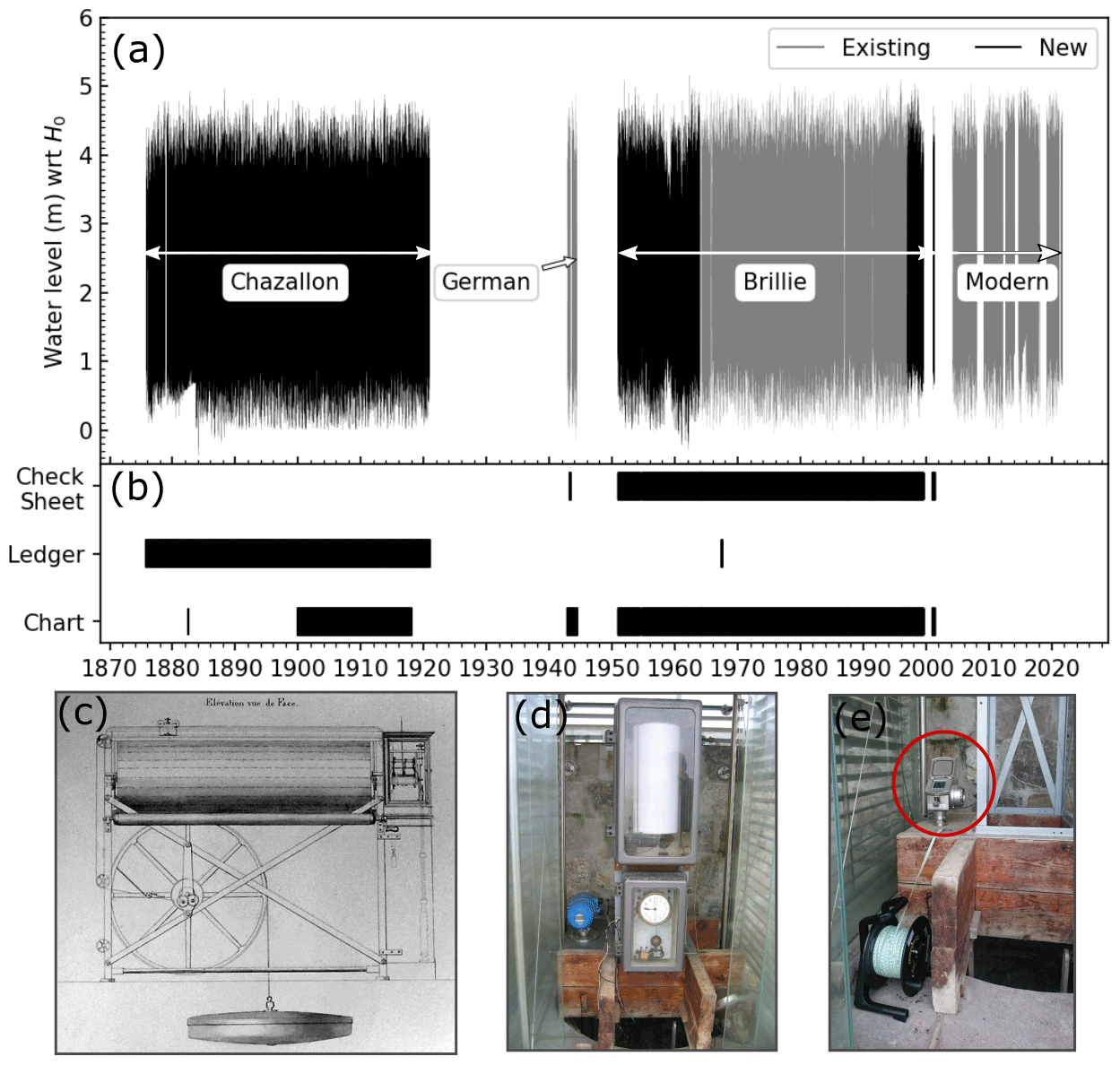
Figure 2 (a) Time series of the water level at Socoa with digitized data (the new datasets from this study are shown in black). (b) Coverage of the rescued registries, charts, and associated check sheets. (c) A schematic of the Chazallon tide gauge (adopted from Pouvreau, 2008). (d) A photograph of the Brillie type tide gauge that was installed until 2004. (e) The modern radar gauge (the photograph was taken by the authors during a field campaign in 2017).

The chronology of the available measurement periods, instruments, recording media, time systems during recording, time sampling before and after digitization, and source archives is summarized in Table 1. The reconstructed time series is in coordinated universal time (UTC), which is further discussed in Sect. 3.2. As the modern instrument record starting in 2004 is not part of the data archaeology exercise, it is not discussed further in the following sections.

Table 1 Overview of the instrumentation periods, original data storage mediums, sampling period of the source and digitized data, and time system of the source observations.

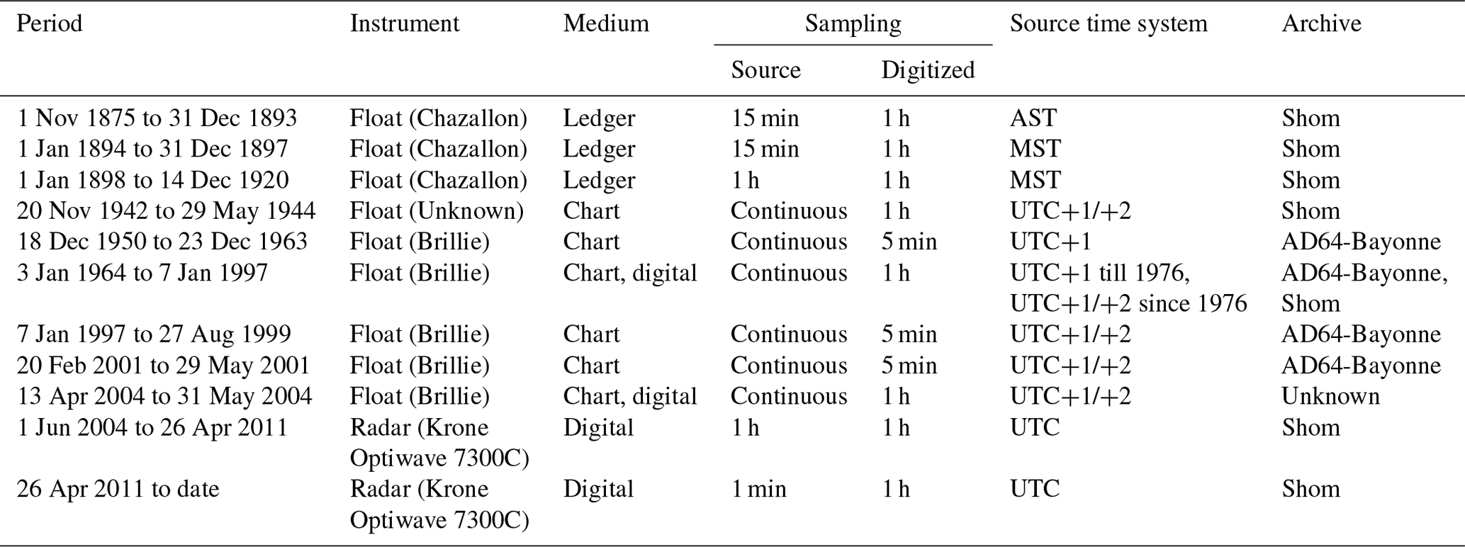
AST: apparent solar time. MST: mean solar time. UTC: coordinated universal time. Shom: Service hydrographique et océanographique de la marine. AD64-Bayonne: Archive Departmental 64 – Pyrénées-Atlantiques – Bayonne.

2.5 Complementary metadata

During the rescue process, administrative documents were found in the archives in which the Socoa tide gauge was mentioned. These documents include tide gauge journals for the Chazallon period containing logs of tide gauge operations, correspondence with the ministry (Ministry of Public Works and Ministry of Marine and Colonies), engineering and hydrographic survey reports, quotes for works, drawings, etc. The hydrographic survey reports were of particular interest for assessing the datum continuity of the tide gauge records (Sect. 3.3). All the documents form an ancillary part of the available metadata and are provided as supplementary files to the dataset (see Sect. 6 on data availability).

3 Digitization and reconstruction of the time series

3.1 Scanning and digitization

The water levels recorded by the Chazallon tide gauge during the 1875 to 1920 period exist in two different media: charts and hand-written ledgers. The large charts were stored for many decades in the archive. They were in an advanced state of deterioration, which prevented them being scanned and rescued. Only the ledgers could be scanned and rescued. The scanned documents are stored as PDF (Portable Document Format) files, each 1–1.2 MB large.

Once the scanning was complete, the process of converting the hand-written text to data (digitization) was done manually, from the scanned document to a computer spreadsheet. The paper for the ledgers was designed for transcribing water levels at 15 min intervals. However, the water levels were only transcribed at 15 min intervals till 1897. Afterwards, the transcriptions were done at 1 h intervals. To speed up the manual digitization process, a choice was made to digitize the water level record at hourly intervals only.

For the Chazallon period from November 1875 to December 1920, 541 ledgers were recovered, corresponding to 45 years of sea level records. More than 390 000 values were digitized manually, which corresponded to several weeks of full-time work. During digitization, the time values were digitized directly as in the ledgers. Sea levels from 1875 to 1893 were recorded in apparent solar time, and from 1894 to 1920 they were recorded in mean solar time. The conversion of these time records into UTC is described in Sect. 3.2.

Unlike the early Chazallon era, the whole recovered archive of the charts covering the 1942–2004 period was scanned (with a photo scanner) and rescued. Most of these charts were accompanied by check sheets. These documents contain relevant information on the time and water level when the chart paper was replaced. The available check sheets were converted into digital form by a photo camera and later used as metadata for identifying problems, especially those related to the slowing down of the clock (see Sect. 4.2).

Prior to this study, an hourly record of sea level at Socoa from 1964–1996 existed in digital form and was available from the Shom data portal (https://data.shom.fr, last access: 30 June 2023). Hence, we applied the water level extraction only to the charts that were outside the range of pre-existing digitized data. From 1950 to 2001, the number of available charts amounts to 777. During the scanning phase, the charts were visually sorted into three categories depending on their condition (good, mildly or badly damaged from mould, and faded) (Fig. S2). Among the 777 charts, 18.3 % (142 charts) were found to be in good condition (Fig. S2). Fifty charts were found to have mild mould (mildly damaged), and 32 charts were found to be widely covered by mould (badly damaged). The majority of the documents, as many as 553 charts (71.2 % of the digitized charts), were found to belong to the third category, with faded water level curve lines.

To extract the water levels from the chart images, specialized open-access software called Numerisation des Niveaux d'EAU (NUNIEAU) was used (Ullmann et al., 2011). For a given chart image, this software can trace the recorded water curve line based on a colour-separation technique. Additionally, the software has built-in features to assign time and height scales in the chart (Fig. S3).

Since the algorithm in NUNIEAU is based on colour separation, the water levels are easier to extract from clean charts. The charts that were in good condition did not need any further image processing to be applied before they were passed through NUNIEAU software. In the second category were the charts which were damaged from mould. These charts were found to be still processable using the processing chain, except for some badly damaged ones which were fully covered by mould. This bad damage essentially translated into a loss of data. Finally, water level curves were very faint in the third category of the charts, and we applied image processing using NUNIEAU (Fig.  S4) to enhance the contrast to process them.

From the charts, the water levels were extracted at the intervals chosen: every 5 min. This time interval corresponds to 20 pixels along the x axis of the scanned charts (scanned at a resolution of 200 dpi). Going below this interval would be pointless as the higher-frequency fluctuations would have been mechanically filtered by the stilling well (IOC, 1985).

The overall process of digitizing ledgers and charts was time-consuming, which is a known characteristic of this kind of data archaeology exercise (Latapy et al., 2022). This is an obvious consequence of manually digitizing the ledgers from scanned documents to a spreadsheet table, but it is a less obvious consequence of the digitization of charts, which is a software-based extraction. In practice, the processing chain could not be automated due to three main reasons. First and foremost, the faded charts needed additional image processing. Second, each chart contained multiple days of water levels which partially overlapped, so dedicated masks were required to separate each day. Finally, the zero of the curves had be set manually for each chart within the NUNIEAU software. As a consequence of these delicate pre-processing steps, the overall chart digitization process was time-consuming, similar to manual digitization from ledgers, as well as challenging to implement in practice.

3.2 Time systems and conversion

Once the scanning and digitization were performed, the next important step was to convert the records into a consistent time system; in this case, the zero-hour time zone of coordinated universal time (UTC), UTC ± 00:00 (henceforth denoted simply “UTC”). Over the recording period of the Socoa tide gauge, the apparent solar time (AST), mean solar time (MST), and legal time systems were used, as listed in Table 1. The following subsections describe the details of the conversion from each time system to UTC.

3.2.1 Apparent and mean solar time

From 1875 to 1893, the ledger records are in local AST. As noted by Wöppelmann et al. (2014), AST was used in the early days of the Chazallon tide gauge era, despite MST being the legal time in France since the early 18th century. Then the records are in local MST until 1920. We first converted AST to MST by adding their difference over the year, known as the equation of time, E, to AST (Hughes et al., 1989; Müller, 1995). Here, E is computed using the formulation published by the Bureau Des Longitudes (2011):

$$\begin{array}{}\text{(1)}& \begin{array}{rl}E& =\mathrm{7.362}\times \sin \left(M\right)-\mathrm{0.144}\times \cos \left(M\right)+\mathrm{8.955}\\ & \times \sin (\mathrm{2}\times M)+\mathrm{4.302}\times \cos (\mathrm{2}\times M)+\mathrm{0.288}\\ & \times \sin (\mathrm{3}\times M)+\mathrm{0.133}\times \cos (\mathrm{3}\times M)+\mathrm{0.131}\\ & \times \sin (\mathrm{4}\times M)+\mathrm{0.167}\times \cos (\mathrm{4}\times M)+\mathrm{0.009}\\ & \times \sin (\mathrm{5}\times M)+\mathrm{0.011}\times \cos (\mathrm{5}\times M)+\mathrm{0.001}\\ & \times \sin (\mathrm{6}\times M)+\mathrm{0.006}\times \cos (\mathrm{6}\times M)-\mathrm{0.00258}\\ & \times t\times \sin (\mathrm{2}\times M)+\mathrm{0.00533}\times t\times \cos (\mathrm{2}\times M),\end{array}\end{array}$$

where t is the time difference from 1 January 2000 00:00:00 (in years; negative for earlier years), and M=6.240060 + 6.283019552×t (in radians). Although the equation given by the Bureau Des Longitudes (2011) is specified for 1900–2100, we have used the same equation for the late 1800s, which induces only minor errors (on the order of seconds). MST was then converted to UTC by adding 404 s, which equals a correction of 4 min for each degree of longitude difference between Socoa and Greenwich (zero longitude).

3.2.2 Legal time

During the Brillie tide gauge period, the measurements were recorded in legal time. The history of legal time in France is long, and we present here a summary of the detailed account of Poulle (1999). Since 1891, the legal time of Metropolitan France was established as the MST in Paris. In a law enacted in 1911, a correction of 9 min 21 s was applied to Paris MST to define the new legal time as Greenwich mean time (GMT). In 1923, the law related to legal time was amended to introduce “summertime” (typically the last Sunday of March to the last Sunday of October), when the clocks are advanced by 1 h. During 1940–1941, timekeeping was different between German-occupied and -free areas. However, during 1942–1944, legal time throughout France was essentially GMT+2 during summer and GMT+1 during winter. Post WW2, France switched to using GMT+1 throughout the year on 18 November 1945. Coordinated universal time (UTC), formulated in 1960, gradually replaced GMT. GMT is essentially equivalent to zero UTC within 1 s. Hence, in the context of this paper, we used GMT+1 and UTC+1 interchangeably. Until 1975, legal time corresponded to UTC+1. In 1976, daylight saving time was adopted again in Metropolitan France, with UTC+2 during summertime (the last Sunday of March to the last Sunday of October) and UTC+1 otherwise, which continues to this day.

In theory, to convert a time record from one time zone to another time zone in GMT or UTC is trivial; it is simply done by accounting for the hour difference of the time zone in question. However, the conversion gets complicated due to clock shifts during the summer and wintertime. For example, it was found that the charts kept recording at the time system (summer or wintertime) of the paper chart installation. The clock was adjusted to the new shifted time when the chart paper was changed. Thus, the metadata associated with these changes were used to properly apply the time difference between legal time and UTC.

3.3 Vertical datum continuity

Since the installation of the tide gauge at Socoa in 1875, the water level has been recorded relative to the “zéro hydrographique” (ZH); that is, the French nautical chart datum. ZH has been in use since the 19th century by French hydrographers (Wöppelmann et al., 2014). A local set of tide gauge benchmarks are usually established around the tide gauge and interconnected by means of levelling to transfer the ZH to each one. Additionally, the practice in France is to include a tide pole and set its zero-measurement mark to the ZH (Wöppelmann et al., 2006b), but this procedure was not adopted for Socoa tide poles. We have found two records of tide poles over the full observation period. For the tide poles, the zero-measurement marks of the poles (ZP) are referenced to different heights from the ZH. Thanks to the rescued documents on the levelling measurements during past hydrographic surveys, it was possible to reconstruct the relationship of the ZH and ZP to current benchmarks and subsequently to assess the continuity of the ZH at Socoa (Fig. 3). The current primary benchmark of the Socoa tide gauge is identified as O.a.K3L3-4-II, which is also part of the national levelling network under the responsibility of the mapping agency (Institut National de l'Information Géographique et Forestière, IGN) (SHOM, 2020).

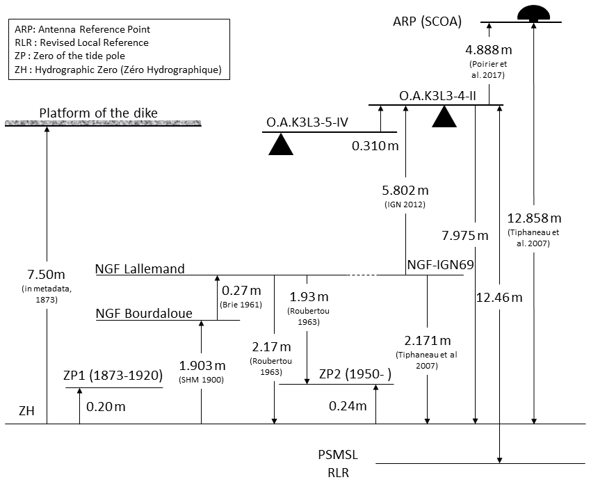
Figure 3 Vertical datum definitions and relationships between benchmarks at the Socoa tide gauge. O.A.K3L3-4-II is the primary benchmark, O.A.K3L3-5-IV is the benchmark shown in Fig. 1e. The references to the measurements are given inside brackets (in small fonts).

The first levelling related to the tide gauge was performed in 1873, which established the ZH as 20 cm below ZP and 7.50 m below the dike level. This information was reported in regional department archive AD64- Béarn (document id: AD64-4S 33) and SHD Vincennes (document id: DD2-2053). In another published document (Annuaire de marées de 1900, Archive Shom), the ZH level was reported to be −1.903 m relative to the first national levelling and the associated datum of France established by Bourdaloue (NGF-Bourdaloue) in 1857–1864. However, it is not clear when this datum connection was made. NGF-Bourdaloue has a difference of 27 cm at Socoa from the second national levelling datum later established by Charles Lallemand during 1880–1922 (NGF-Lallemand), locating the hydrographic zero at −2.17 m relative to the NGF-Lallemand datum (Brie, 1961). No other report of levelling surveys was found during the Chazallon tide gauge period.

In a hydrographic survey done in 1961, the ZH was estimated as being 18 cm above the originally established ZH (Brie, 1961). A follow-up investigation in 1963 revealed that the tide gauge was suffering from heavy siltation and the connection to the sea was blocked during the survey of 1961, causing the deviation (Roubertou, 1963). Following the investigation in 1963, the ZH was maintained at −2.17 m NGF Lallemand, and the ZP was measured to be 24 cm above the ZH.

All available documents suggest there was no change in the definition of ZH at Socoa. One false alarm was a letter dated 9 October 1968 and addressed to Shom, where it was mentioned that “the zero of the tide pole” (le zéro de l'échelle) was located at −2.178 m relative to the NGF Lallemand datum, and the primary benchmark was located 5.822 m above the NGF Lallemand datum. This was identified as a mistake based on the survey done in 2007, which measured the height of OaK3L3-4-II to be 5.805 m IGN69 (Tiphaneau et al., 2007). IGN69 refers to the current national levelling datum (NGF-IGN69), which was established by the IGN during 1962–1969. The reported difference between the datum of NGF Lallemand and NGF-IGN69 at Socoa is 0 m (grid 1245, https://geodesie.ign.fr/contenu/fichiers/grillesorthonormales/GrilleOrthoNormale_Ouest.pdf, last access: 19 July 2020). Currently, the hydrographic zero (ZH) is reported to be 7.975 m below the OaK3L3-4-II benchmark and 2.171 m below NGF-IGN69 datum (Poirier et al., 2017). One of the nearby secondary benchmarks, OaK3L3-5-IV (Fig. 1e), sits 0.310 m below OaK3L3-4-II (Fig. 3).

4 Data quality assessment

In the previous section, we discussed the method used to reduce the records to a common time system and vertical datum (ZH). These two steps resulted in a merged time series, which was subsequently assessed to detect any potentially erroneous or suspicious water levels (IOC, 2020). Several methods, described in the following subsections, were used to identify potential problems in the data. Based on the rescued metadata, a correction was applied wherever possible, and the corresponding data were flagged.

4.1 Data quality flag

The flag value is defined as a 4-bit number in which 1 means the flag is on and 0 means off. Each bit from left to right corresponds to the following:

• Bit 1 – time correction is applied;

• Bit 2 – height correction is applied;

• Bit 3 – low confidence in the correction in time or height;

• Bit 4 – documented siltation period.

For example, the 4-bit flag 1010 reads as follows: a time correction is applied (the first bit is 1 = true) without height correction (the second bit is 0 = false), but the data are suspected to be bad (the third bit is 1 = true), even though no siltation was reported (the fourth bit is 0 = false). This concept is similar to the flag accompanying the PSMSL data (https://www.psmsl.org/data/obtaining/psmsl.hel, last access: 30 June 2023).

Two files in the Supplement list the corrections done on the raw data for the ledgers (corrections_registry.csv) and the charts (corrections_marigram.csv), respectively. These are concatenated into one file named “correction.csv” for analysis, which is henceforth identified as the “correction file” (see Sect. 6 on data availability). In the following sections, different quality control steps are discussed.

4.2 Quality control and corrections

Several basic quality control methods based on visual inspection were applied during the time series construction process. For the ledger data, the digitized tabulated values in spreadsheets were colour-coded, with the colour ranging between maximum and minimum values to enable the visual identification of errors (see Fig. S5). One of the common errors that this procedure highlights is that the transcription of the height can be wrong by 1 m (and sometimes by 2 m). These corrections are flagged as height corrections (i.e. the second bit is 1 in the flag).

Once the obvious height corrections had been applied, a tidal harmonic analysis based on validated data was performed, and the recorded water levels were compared with the predicted water levels visually week by week (Pugh and Woodworth, 2014). This comparison process was useful for identifying days with a wrong date (switched with the previous or the following curve in the chart) during transcription as well as incorrect high and low tides with respect to the tide gauge journal (Sect. 2.5). The tide gauge journal was checked, and corrections were made if necessary. The high and low tide corrections were typically between 10 and 20 cm.

For the digitized charts, the check sheets were consulted before the time series extraction using NUNIEAU. Time anomalies where the last time of measurement on the chart was different from the one indicated in the check sheet were noted for some charts. This type of anomaly is likely due to the faulty placement of the chart on the rotating drum, causing a time difference for the entire measurement period covered by the chart (typically of the order of 5 min). The time information on the check sheets was used to apply a time correction. Whenever a constant difference between the time on the check sheet and the tide gauge was noted, a time shift was applied to the final dataset. When the time shift was different at the beginning and the end, the minimum value of the time shift was applied to the final data. In some cases, the hourly grid scale in the charts was relabelled by the observer. The changes induced by grid relabelling were applied directly in the parameterization of NUNIEAU, rather than applying them later.

The above quality controls resulted in a corrected dataset with variable time steps depending on the source (ledgers, charts), which was further sampled to hourly values using a linear interpolation. During interpolation, the missing values were computed only if the interpolated timestamp was surrounded by valid data points. This interpolated hourly dataset is the main outcome of this data archaeology exercise and is used in the subsequent analysis (see also Sect. 6 on data availability).

4.3 Unresolved data quality issues

During the processing of the charts, some additional issues were noticed that could not be corrected. These included occasional slowing down of the clocks, mismatching between the height measured by the chart and the tide-pole reading (reported in the check sheets), and a delayed rising or falling tidal curve (Fig. S6). Furthermore, siltation was noted to be a major problem at this tide gauge station. These issues are addressed below.

4.3.1 Slowing down of the clock

Thanks to the check sheets, it was possible to cross-check the consistency of the clock at the beginning and the end of a recording period of a chart (Fig. S6). In some cases, the start time of the clock was found to be correct but the clock showed a slowing down at the end. The magnitude of the difference varied from 1 to 10 min. Only a small portion of the data (less than 2 %) were affected by this problem. Given the length of the record in each chart (typically 8–10 d), it was difficult to apply a correction confidently. These values were flagged as values with low confidence (i.e. the third bit in the flag was set to 1).

4.3.2 Possible malfunctioning of the float device

In some instances, the tidal curves displayed a quasi-linear rise/fall instead of the characteristic sinusoid-like evolution (Fig. S8). This suggests a malfunction of the mechanical system. In all these cases, the tide gauge regained its normal behaviour in the next tidal cycle. Less than 1 % of the recovered data presented this problem. Another issue was linked to siltation (see the next subsection), which impacted the movement of the float. This concerned about 8 % of the total recovered hourly data. The values impacted by this issue were also flagged as values with low confidence (i.e. the third bit in the flag was set to 1).

4.3.3 Siltation

One of the main known issues for the Socoa tide gauge is the siltation of the stilling well (Roubertou, 1963; Poirier et al., 2017). The geometry of the stilling well is shown in Fig. 4a. The stilling well (Fig. 4b) is connected through a pipe 8 cm in diameter. The first major siltation problem with the data recording was noticed within the first few years of operation. Notably, the accumulation of silt inside the stilling well restricted the movement of the float (see the previous subsection) and impacted the recording of low water levels (less than 70 cm). Significant maintenance work was undertaken during 1883–1884 to improve the connectivity of the stilling well to the ocean by creating a duct (Fig. 4a, d). The entrance shown in Fig. 4c and d was apparently open and accessible through a wooden door. At some (unknown) point, the entrance was partially closed and the connectivity with the stilling well was severed. After restarting the operation of the tide gauge in 1950, the stilling well again exhibited siltation and blockage-related problems (Robertou, 1963).

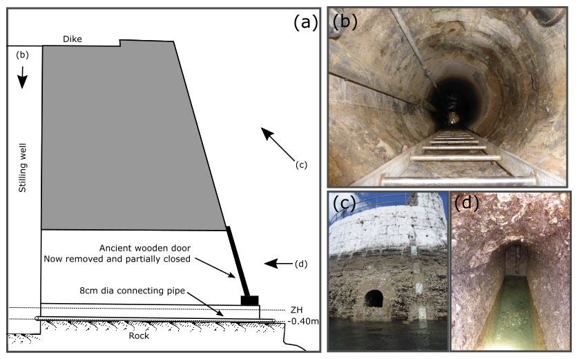
Figure 4 (a) Schematic of the current stilling well. (b) View inside the stilling well from above. (c) Entrance to the stilling well (at about 1m above the water level). (d) Inside the passage to the stilling well from the entrance. The images were collected during fieldwork in 2017 (Poirier et al., 2017).

As noted in the literature (e.g. Pugh and Woodworth, 2014), malfunctioning of the instrument can be detected by examining the tidal constituents. More specifically, a blockage related to siltation can be detected as a simultaneous amplitude attenuation and phase delay (e.g. Wöppelmann et al., 2014). Here, we computed the changes in M2 tide from a running tidal harmonic analysis with yearly segments from 1875 to 2020 using Utide (python) version 0.2.6 (Codiga, 2011, https://github.com/wesleybowman/UTide, last access: 26 January 2022). Figure 5 shows the M2 amplitude and Greenwich phase lag, with the error bars representing the 95 % confidence intervals. The most apparent impact of siltation on the tide can be observed during 1956–1963 in Fig. 5, which is supported by a report of hydrographic surveys carried out at that time (Robertou, 1963). Another simultaneous amplitude attenuation and phase delay can also be spotted around the end of the 1990s (1997–2000).

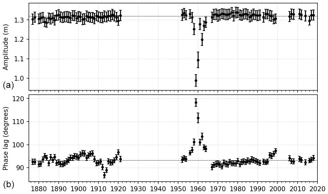
Figure 5 M2 amplitude (a) and Greenwich phase lag (b) calculated for 1-year segments using tidal harmonic analysis. The dotted lines correspond to the amplitude and phase lag computed for the whole time series. Error bars are 95 % confidence intervals.

We have flagged (i.e. the fourth bit was set to 1) the data that were deemed to be impacted by the siltation problem. Based on the above-mentioned harmonic analysis, the data from 1955–1963 and 1998–1999 are flagged. We also added the siltation flag to the data from 12 November 1875 to 31 August 1883 based on the metadata. In total, about 29 % of the total recovered hourly data are flagged as being impacted by siltation.

The siltation problem discussed above persists to this day. Currently, the stilling well is cleaned, typically yearly, to maintain acceptable quality of the data. However, access to the stilling well is challenging, and the cleaning operation is costly. The maintenance is also often perturbed by administrative complications and unforeseen events (e.g. the Covid-19 lockdown in 2020–2021). Also, under current conditions, the stilling well does not conform to the recommended 2 m depth of water at lowest astronomical tide (IOC, 2016). For the Socoa tide gauge, which is currently equipped with a guided wave radar, we recommend a transition from the installation on the stilling well to an installation mounted on the quay of the dike with an unguided open-air radar tide gauge.

4.4 Assessment of the vertical datum continuity

One of the commonly used quality control techniques for sea level is so-called “buddy checking”, which relies on a comparison with mean sea level time series from nearby sites (Pugh and Woodworth, 2014). The difference in monthly mean sea level from a nearby tide gauge essentially removes the common part of the spatially coherent modes of variability and can reveal malfunctioning at one of the gauges – for instance, step-like features associated with a vertical datum discontinuity (Woodworth, 2003; Hogarth et al., 2020). Here, we compare our record with the sea level record from the Brest (obtained from https://data.shom.fr, last access: 26 January 2022) and Santander (obtained from PSMSL, https://www.psmsl.org/, last access: 10 April 2022) tide gauges. The Brest tide gauge data are a well-validated long time series (starting in the 17th century) for this region (Wöppelmann et al., 2006a, 2008) that covers the whole time series of Socoa. For Santander, Marcos et al. (2021) extended the Santander time series through data archaeology back to 1875 (see Fig. S9). However, there are multiple apparent datum shifts in the data during the early years (1875–1910), so we refrained from discussing the extended time series in the buddy checking for Socoa.

We adopted the PSMSL processing scheme for computing the monthly means for Socoa and Brest. First, a Demerliac filter was applied to the hourly data to obtain a detided hourly time series for Socoa and Brest. From the hourly detided water level, the daily mean sea level was obtained using daily averages. A monthly mean was computed only if 50 % or more of the data were available. As the Santander dataset was directly obtained from the PSMSL, no further pre-processing was necessary.

The differences between the monthly mean sea levels at Socoa and those at Brest and Santander are shown in Fig. 6. For comparison, the mean (computed over 1965–2000) was removed from each dataset before computing the difference. Note that the periods with suspected siltation issues (Sect. 4.2.3) were removed from the Socoa time series for this analysis.

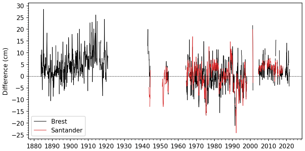
Figure 6 Difference between the monthly MSL at Brest (black) or at Santander (red) and that at Socoa. The mean over 1965–2000 was removed from each station for comparison.

From Fig. 6, no persistent step-like feature is seen in the Brest minus Socoa time series (black), which further strengthens our confidence in the vertical datum continuity established in Sect. 3.3. In Fig. 6, it is interesting to note the gradually increasing difference during the early 20th century. In the literature, this decadal feature is shown to be linked to a large-scale sea-level variability coherent with atmospheric modes of the North Atlantic (Woodworth et al., 2010b; Sturges and Douglas, 2011; Calafat et al., 2012; Chafik et al., 2019), and is explained by the steric response (Calafat et al., 2012). Both the Brest and Socoa tide gauges show this decadal variability (see Fig. S9), but with a lower amplitude at Socoa compared to Brest, hence producing the increasing positive difference from 1900 to 1915 in Fig. 6.

The Santander minus Socoa time series also does not indicate any datum shift and is generally consistent with the Brest minus Socoa time series. However, we see a small consistent deviation of 5 cm on average during 1976–1980.

5 Trend analysis

From the hourly time series for Brest and Socoa, we have computed yearly means using the yearly PSMSL rules (at least 11 monthly means for a year) and estimated the trends and associated 1-sigma uncertainty (Table 2).

Over the same period (1900–2018), the trend is 1.50±0.09 mm yr⁻¹ for Brest and 2.12±0.11 mm yr⁻¹ for Socoa. The benefit of a long time series is clear here – the longer the time series, the smaller the uncertainty. To compare with the previously published result from Marcos et al. (2021), we also computed the trend for the non-detided time series shown in Fig. S9, as listed in Table 2 under the corresponding period with two asterisks (**). The trend estimate is very similar for Socoa and Santander during the common period: 2.08±0.20 mm yr⁻¹ for Socoa and 2.01±0.12 mm yr⁻¹ for Santander.

Table 2 Estimated linear trends in mm yr⁻¹ at Brest and Socoa over various time periods, computed from yearly mean time series.

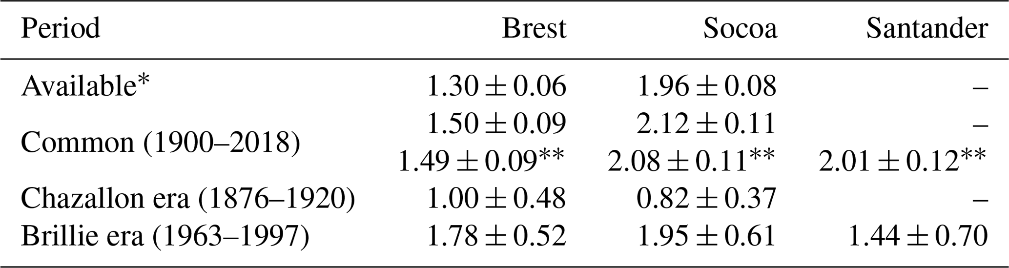
^* The available period for Brest is 1846–2021; that for Socoa is 1875–2021. ${}^{**}$ Computed from the annual mean sea level without using a tide-killer filter (Demerliac).

In the last two rows of Table 2, the estimated trends computed over two periods separated by 40 years – the Chazallon era (1876–1920) and the Brillie era (1963–1997) – are shown. The sea level trend at Socoa during the Brillie era (1.95±0.61 mm yr⁻¹) is noticeably increased (i.e. accelerated) compared to the Chazallon era (0.82±0.37 mm yr⁻¹). A similar magnitude of the trend is found at Brest too. During the Chazallon era, the trend at Brest is higher compared to that at Socoa, which is opposite to what is seen for the Brillie era. Analysis of the factors that contribute to this observed change in trend is out of the scope of this data paper. However, this leads us to another benefit of a long time series: it allows the investigation of the non-linear evolution of mean sea levels and associated trends. This benefit is illustrated below through the analysis of inflexion points in the trends at Socoa and Brest.

The analysis is motivated by Wöppelmann et al. (2006a), who noted an inflexion point around 1890 at Brest, which is close to the inflexion point estimated for Liverpool around 1880 by Woodworth (1999). To find the inflexion point of the trend, we have analysed the same yearly time series at Socoa and Brest as above. A linear trend analysis was applied over a running window of 20 years. Windows containing two or more consecutive missing values were removed from the analysis. The trend (mm yr⁻¹) and 1-sigma uncertainty range are shown in Fig. 7. We reproduce an inflexion point at around 1887 in Brest and an estimated inflexion point between 1895–1900 in Socoa.

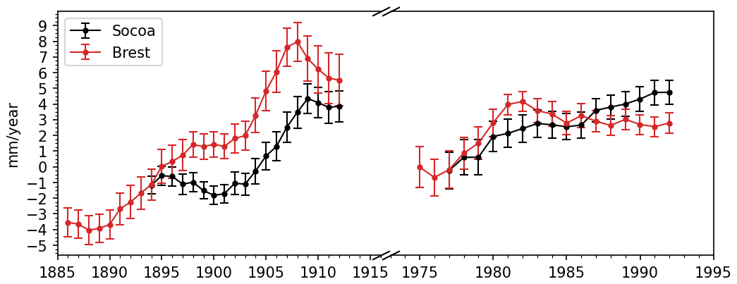
Figure 7 Running trend estimates (20 year windows) for Socoa (black) and Brest (red) during 1875–2000. Each error bar shows the 1-sigma uncertainty range of the trend estimate. Break lines indicate the skipped period (when not enough continuous data were available for the analysis).

Multiple drivers may contribute to this inflexion point – decadal variability, long-term climate variability, and climate-change-induced sea level acceleration. The decadal sea level variability during the early 20th century, which is potentially the main contributing factor to the inflexion point in the trend, is found to be linked with the atmospheric modes of the North Atlantic (Calafat et al., 2012). Jevrejeva et al. (2008) show that there is a prominent 60 year climatic variation in the trend (acceleration-deceleration) and, during the analysis period (1875–1929), the global pattern is a deceleration until around 1910. However, the North-East Atlantic shows a strong deviation from the global pattern, with an earlier switch to acceleration at around 1900 (Jevrejeva et al., 2008, Fig. 3). Finally, the exact timing of the start of the global acceleration of the trend due to sea level rise has not been accurately answered yet, but studies point to sometime in the early 19th century (Church and White, 2006; Jevrejeva et al., 2008). Hence, the global trend in sea level rise may have further contributed to the timing of the inflexion point.

6 Data availability

The raw digitized water level, the processed dataset, metadata, and the python notebooks used for processing are openly available at https://doi.org/10.5281/zenodo.7438469 (Khan et al., 2022). The data repository is organized into four sub-directories:

• data/ contains the raw and processed dataset for Socoa (data/socoa) and another auxiliary dataset (data/auxiliary) used in the analysis.

• documents/ contains an inventory of the ledgers and charts (documents/inventory.xlsx), transcripts of metadata extracted from the regional archives (documents/archive_records), and selected transcripts from the tide gauge journal during the Chazallon era (documents/tidegauge_journal).

• figures/ contains the generated figures used in the article.

• notebooks/ contains the Python notebooks used to process and analyse the data.

The final hourly time series of the water level in metres vertically referenced to local hydrographic zero (ZH) with the data quality flags discussed in this paper is distributed as a comma-separated values file (data/socoa/socoa_L4.csv) with metadata in the header. The dataset starts at 1 November 1875 and stops at 4 October 2021 and contains 101 years with data.

In documents/, the transcriptions of the relevant part of the tide gauge journals are provided with the data as yearly documents. The excerpts of metadata documents from the archives of the Service Historique de la Défense (SHD) at Brest (SHD-Brest), Rochefort (SHD-Rochefort), and Vincennes (SHD-Vincennes), the Archives des Pyrénées-Atlantiques – Béarn (AD64-Béarn), the Archives des Pyrénées-Atlantiques – Bayonne (AD64-Bayonne), and the SHOM archive are also provided as supplementary files to the dataset.

This dataset can be reproduced by applying time and height corrections to the raw uncorrected water level records for Socoa (data/socoa/socoa_raw.txt), using the data processing script (notebooks/01_data_processing.ipynb) and the corrections (data/socoa/corrections.csv). Further details about the files available in the data repository can be found in the included README.md text file.

A continuously updated time series of the Socoa sea level can be obtained from the Shom portal (https://doi.org/10.17183/REFMAR#95, SHOM, 2023).

7 Conclusions

We have done a thorough archival research, data rescue, digitization, and metadata analysis and increased the coverage of the existing hourly sea level record at Socoa, Saint-Jean-de-Luz (France) back to 1875. Among the total of 702 station-months of additional data, 693 station-months have more than 50 % data per month. This increase in data amounts to about 58 years' worth of new data.

Data quality flags were assigned to the recovered and distributed final hourly dataset based on a careful inspection of the metadata and a dedicated analysis of the dataset. The amount of data for which time and height corrections were needed and applied with confidence is small (less than 2 % in total). Additional flags were assigned to indicate when time or height corrections were applicable but could not be applied confidently due to insufficient information. A very small proportion of the data (<1 %) is affected by this issue (without considering siltation-related problems).

The most common reason for flagging data was siltation in the stilling well. A dedicated analysis of the data and metadata was done to identify and document periods with siltation. We have identified three main periods: 1875–1893, 1951–1963, and 1998–1999. A dedicated flag was assigned to these periods, which correspond to 29 % of the recovered hourly data.

Considering the gravity and the recurrent nature of the siltation problem in the stilling well, we recommend a transition from the stilling well to an open-air installation for this tide gauge. This transition should be supplemented with a study of the filtering characteristics of the stilling well to track any impact of the installation change on future sea level measurements.

The extended dataset will be communicated and deposited in international sea level databanks (e.g. PSMSL) to further increase the number of long-term sea level records extending back into the 19th century. One of the major features of this sea level record is its location, which has remained the same (in terms of buildings and stilling well) since its installation in 1875. The data recovered and rescued in this work would be useful for long-term sea level trend analysis (e.g. Gehrels and Woodworth, 2013) and modelling at decadal to interannual scales (e.g. Calafat et al., 2012; Ding et al., 2021). Investigations of extreme events will especially benefit from the high temporal sampling of the extended time series.

Besides the final hourly sea level dataset from 1875 to 2021, we also provide the raw data, associated corrections that are synthesized above, and computational notebooks as companion datasets (see Sect. 6). The objective of this is to promote reproducible research and to increase transparency by allowing the validation of our computations.

In this data paper, we have not only extended the sea level time series at Socoa but also showed that analysing the history of individual tide gauges can reveal important location-specific issues, like siltation, that might not be directly evident from the global dataset at this moment. During the current data archaeology work, we have also found unrecoverable deterioration of historical paper documents, which underlines the urgency of rescuing these invaluable records. Relevant metadata are also in the same danger of being deteriorated beyond rescue.

Finally, there is a vast amount of untapped tide data and associated metadata worldwide (Pouvreau, 2008; Bradshaw et al., 2015; Talke and Jay, 2017). Talke and Jay (2017) reported the identification of more than 6500 station-years of previously lost or forgotten tide data across the United States. Over 60 000 identified documents have been inventoried in France (see the Shom inventory, http://refmar.shom.fr/dataRescue, last access: 30 June 2023); 70 % of those have already been rescued (e.g. scanned), but many remain undigitized (Latapy et al., 2022). Given the time-critical risk of losing this valuable scientific and historic information, it is crucial to urgently rescue these datasets, digitize them, and make them available to the scientific community.