the Creative Commons Attribution 4.0 License.
the Creative Commons Attribution 4.0 License.
 | 12 Dec 2023
A long-term dataset of simulated epilimnion and hypolimnion temperatures in 401 French lakes (1959–2020)
Najwa Sharaf
Jordi Prats
Nathalie Reynaud
Thierry Tormos
Rosalie Bruel
Tiphaine Peroux
Pierre-Alain Danis
Understanding the thermal behavior of lakes is crucial for water quality management. Under climate change, lakes are warming and undergoing alterations in their thermal structure, including surface water and deepwater temperatures. These changes require continuous monitoring due to the possible major ecological implications for water quality and lake processes. We combined numerical modeling and satellite thermal data to create a regional dataset (LakeTSim: Lake Temperature Simulations) of long-term water temperatures for 401 French lakes in order to tackle the scarcity of in situ water temperature (Sharaf et al., 2023; https://doi.org/10.57745/OF9WXR). The dataset consists of daily epilimnion and hypolimnion water temperatures for the period 1959–2020 simulated with the semi-empirical OKPLM (Ottosson–Kettle–Prats Lake Model) and the associated uncertainties. Here, we describe the model and its performance. Additionally, we present an uncertainty analysis of simulations with default parameter values (parameterized as a function of lake characteristics) and calibrated parameter values along with the analysis of the sensitivity of the model to parameter values and biases in the input data. Overall, the 90 % confidence uncertainty range is largest for hypolimnion temperature simulations, with medians of 8.5 and 2.32 ∘C, respectively, with default and calibrated parameter values. There is less uncertainty associated with epilimnion temperature simulations, with medians of 5.42 and 1.85 ∘C, respectively, before and after parameter calibration. This dataset provides over 6 decades of epilimnion and hypolimnion temperature data crucial for climate change studies at a regional scale. It will help provide insight into the thermal functioning of French lakes and can be used to help decision-making and stakeholders.
- Article
(4967 KB) - Full-text XML
-
Supplement
(484 KB) - BibTeX
- EndNote


Lakes, both natural and artificial (i.e., reservoirs and gravel pits), are sentinels of environmental change and provide important services such as access to drinking water, hydropower production, recreation and fisheries (Adrian et al., 2009). Under climate change and anthropogenic pressures, many lakes are warming and consequently experiencing changes to their biophysicochemical structure and function that are leading to services being compromised (Janssen et al., 2021).
In lakes, water temperature is an essential parameter regulating processes such as the functioning of trophic webs, oxygen conditions, the physical structure of the water column and the biogeochemistry (Yang et al., 2018). Under warming, historical records and future projections demonstrate that, for lakes, alterations in the thermodynamic functioning including warmer temperatures and shifts in mixing regimes have already taken place and are expected to persist in the future (Shatwell et al., 2019; Woolway and Merchant, 2019). In this context, they are undergoing shorter periods of ice cover and longer, more stable periods of thermal stratification (Woolway et al., 2022). These alterations could have considerable ecological implications for the biological communities (Lind et al., 2022; Havens and Jeppesen, 2018). For instance, worldwide studies have shown that the expansion of toxic cyanobacterial blooms is linked to warming (Griffith and Gobler, 2020). Other responses include species reduced body size (Daufresne et al., 2009), changes in thermal habitat and shifts in species seasonality (Kharouba et al., 2018).
It is thus crucial to closely evaluate water temperature trajectories over the entire water column in space and time when assessing the impact of climate change on lake ecosystems. However, the lack of data coverage, both spatially and temporally, makes it difficult to accurately characterize lake thermal response to climate change and to identify warming trends (Gray et al., 2018). Indeed, long-term datasets of in situ temperatures are usually scarce and mostly limited to large lakes (Layden et al., 2015). Moreover, the sampling frequency and temporal coverage of in situ water temperature vary greatly from one lake to the next, from a few years (Sharma et al., 2015) up to decades (Piccolroaz et al., 2020; Rimet et al., 2020).
Due to the difficulties in setting up conventional (i.e., in situ) monitoring programs tied to, e.g., costs, governance and intercalibration, the coupling of modeling and satellite remote-sensing data has become fundamental in the field of limnology (Nouchi et al., 2019). Modeling provides a means of interpolating both temporal and spatial gaps. It thereby allows us to acquire information about surface water temperatures, which are globally the focus of lake climate change studies and deepwater temperatures, which are as critical though often disregarded in this context (see however Pilla et al., 2020). Several numerical models that vary in complexity exist for conducting water temperature simulations, the most accurate being deterministic or process-based models. Nevertheless, regional or global deterministic modeling efforts over long periods are usually hindered by the lack of sufficiently detailed input data (e.g., meteorological and field data) to run the models (Kim et al., 2021). For practical and operational purposes, simpler models (semi-empirical, statistical or hybrid physical–statistical-based models) with fewer requirements for forcing data have mostly been applied to assess the impact of climate change on lake ecosystems and to study them (Piccolroaz et al., 2020; Toffolon et al., 2014; Sharma et al., 2008). Long-term simulations across a considerable number of lakes are made possible with this type of model, enabling the detection of trends in time series data that are not achievable with shorter datasets (Gray et al., 2018).
The performance of numerical models depends highly on the calibration of their parameters as well as on the quality of the input data. Satellite remote sensing is an effective way of monitoring surface water temperature on a synoptic scale (Schaeffer et al., 2018; Sharaf et al., 2019) and providing a complementary source of data to in situ measurements for model calibration or validation purposes (Allan et al., 2016; Babbar-Sebens et al., 2013). In particular, thermal infrared sensors on board the Landsat satellites are very adequate for retrospective analysis of surface water temperature with a spatial resolution adapted for small- to medium-sized lakes and reservoirs at a bimonthly acquisition frequency. Landsat 4 and 5 TM (Thematic Mapper), 7 ETM+ (Enhanced Thematic Mapper) and 8 TIRS (Thermal InfraRed Sensor) provide surface temperature data at spatial resolutions of 120, 60 and 100 m, respectively. Landsat series records of surface water temperature can be used to validate 3D hydrodynamic models when in situ measurements are scarce (Sharaf et al., 2021) and to spatially assess the quality and suitability of the aquatic habitat for biological communities (Halverson et al., 2022). Although satellite thermal data are limited to the surface, their integration into model calibration could improve the accuracy of simulations over the surface layer and the water column (Javaheri et al., 2016).
Here we present, on a regional scale, a long-term dataset, LakeTSim (Lake Temperature Simulations), of daily epilimnion and hypolimnion temperature simulations as well as uncertainties for the period 1959–2020 over 401 French lakes monitored under the Water Framework Directive (WFD) including natural and artificial lakes, reservoirs and gravel pits. We present the OKPLM (Ottosson–Kettle–Prats Lake Model) used to produce water temperature simulations and its performance. Further, we provide an uncertainty analysis of simulations with default (parameterized with in situ and satellite thermal data over an entire set of lakes) and calibrated (with in situ temperature measurements for each lake) model parameter values as well as a sensitivity analysis for the latter. The goal of publishing this dataset is to provide new insight into epilimnion and hypolimnion temperatures of lakes in France, especially for those that are not monitored regularly through conventional methods. This long-term dataset is valuable for developing temperature indicators for identifying warming trends, extreme events and possible changes in the mixing regime, among others. These indicators will contribute to assessing the impact of climate change on lake thermal functioning and its influence on the biological community structure and trophic webs.
2.1 The ALAMODE (A LAke MODElling project) software suite
The simulation, sensitivity and uncertainty analyses presented in this paper were done using the ALAMODE software suite. ALAMODE (Danis, 2020) is a software suite developed in Python 3 by the Pôle R&D Ecosystèmes Lacustres (ECLA) and SEGULA Technologies to facilitate the realization of simulations of lakes and the management of related information. It comprises multiple modules and packages designed for lake and tributary modeling as well as for processing the data necessary to operate these models. These packages include the OKPLM, CUSPY (Calibration, Uncertainty analysis and Sensitivity analysis in PYthon), TMOD (Temperature MODelling), GLMtools (General Lake Model tools), “tributary”, TINDIC (Temperature INDICators) and ALAPROD (ALAMODE-Production). The OKPLM (Prats-Rodríguez and Danis, 2023b) is used to simulate epilimnion and hypolimnion water temperatures in lakes, while CUSPY (Prats-Rodríguez and Danis, 2023a) is used for model parameter estimations and conducting uncertainty and sensitivity analyses. TMOD is used for managing the TMOD database designated to facilitate the realization and consultation of simulations. GLMtools is used to conduct lake hydrodynamic simulations using the one-dimensional hydrodynamic General Lake Model (Hipsey et al., 2019), while tributary is used for the estimation of the flow and temperature of lake tributaries. The TINDIC package is used to calculate temperature indicators from model simulations. Finally, ALAPROD integrates all the functionalities to produce simulations into a single package: simulation of stream water temperature, of lake hydrodynamics and temperature, and of streamflow rate. It also includes sensitivity and uncertainty analysis features. The functionalities of these packages can be accessed either by using each package separately or by utilizing the ALAPROD package, which depends on the TMOD database and requires access to it.
At present, only the ALAMODE packages related to the main functionalities used in this work are publicly available (see the “Code availability” section): the simulation of lake temperatures using the OKPLM (Prats and Danis, 2019), implemented in the OKPLM package, and the sensitivity and uncertainty analysis tools in the CUSPY package. We used ALAPROD to access the functionalities of both packages.
2.2 The OKPLM description
The OKPLM (Prats and Danis, 2019) is a two-layer semi-empirical data model adapted from Kettle et al. (2004) for the epilimnion module and from Ottosson and Abrahamsson (1998) for the hypolimnion module. The modifications proposed in Prats and Danis (2019) consisted mainly of simplifying the mixing algorithm used in Ottosson and Abrahamsson (1998) using a basic stability condition, whereas for the epilimnion module a sinusoidal fit to the average daily solar radiation was used instead of the theoretical clear-sky radiation. The OKPLM also runs on weekly and monthly frequencies. The regionalization of the parameters of the model mainly depends on the geographical and morphological properties of the lake (maximal depth, volume, surface area, latitude and altitude). The model requires few meteorological forcing data: solar radiation and air temperature.
The model calculates water temperature as follows:
where Te is the epilimnion temperature (∘C); i is the day number; A, B and C are calibration parameters; S is the solar radiation (W m−2); and f(∗) is an exponential smoothing function with defined as
where Ta,i is air temperature (∘C) and MAAT is the mean annual air temperature (∘C). The smoothing function f(∗) is such that it gives greater weight to the nearest observations and the weights decrease exponentially. It is defined as
where α is the smoothing factor. When α=1, there is no smoothing, while the smoothing increases with the decrease in the value of α.
where Th is the hypolimnion temperature (∘C), D and E are calibration parameters and g(Te,i) is an exponential smoothing as follows:
where β is the exponential smoothing factor. As for α, there is no smoothing for β=1, and the smoothing increases as β approaches zero.
In ALAPROD, the OKPLM can be run in two modes: the “default” mode where model parameter values for each lake are estimated using the parameterization presented in Prats and Danis (2019) and the “calibrated” mode where model parameters are calibrated individually for each lake by using in situ temperature measurements. The default parameterization was obtained by using the individually calibrated parameter values to fit appropriate expressions as a function of the characteristics of lakes. In the epilimnion module, model parameter values A, B, C and α are estimated based on lake characteristics (i.e., latitude, altitude, surface area, volume and depth). These equations were determined using robust regressions and Landsat infrared data (median skin temperatures) from 1999 to 2016 of French lakes to estimate mean surface temperatures (Prats et al., 2018). In contrast, for the hypolimnion module, parameter values E and β were derived as a function of lake depth and lake type using temperature profile data from 357 lakes; β can have values of 1 (E>0.95) or 0.13 (E≤0.95). Parameter D was assigned a constant value of 0.51.
The parameterization of the OKPLM parameters as presented in Prats and Danis (2019) is as follows:
where LLat is lake latitude (∘ N), LAlt is lake altitude (m) and LA is lake surface area (m2).
where LDmax is lake maximal depth (m).
where e1, e2 and e3 are coefficients with respective values of 0.10, 2.0 and −1.8 for natural lakes and 0.49, 1.7 and −2.0 for artificial lakes (reservoirs, gravel pits, ponds and quarry lakes), and LD is lake mean depth (m).
where LV is lake volume (m3).
2.3 Input data
The OKPLM was forced with two sources of meteorological data extracted from the SAFRAN (Système d'Analyse Fournissant des Renseignements Adaptés à la Nivologie) analysis system (Durand et al., 1993) and the S2M (SAFRAN–SURFEX/ISBA–Crocus–MEPRA; Modèle Expert d'Aide à la Prévision du Risque d'Avalanche) meteorological reanalysis (Vernay et al., 2015, 2022).
The SAFRAN system provides meteorological variables at an hourly time step estimated through interpolation and assimilation processes with an 8 km square grid. Average daily data from the nearest grid cell were selected for each study site. The difference in altitude between the study site and the grid cell was accounted for by applying an adiabatic elevation correction to air temperature.
The S2M model chain combines the SAFRAN meteorological analysis and the SURFEX/ISBA–Crocus snow cover model including MEPRA. It is more adapted to mountainous regions as it has a spatial definition where spatial heterogeneity is taken into consideration. The S2M reanalysis uses a vertical resolution of 300 m and is the result of simulations performed over mountainous zones referred to as “massifs” and covering the French Alps, Pyrenees and Corsican mountainous regions. In order to use S2M meteorological data over each lake, an extraction of certain topographic classes is necessary. These include elevation, aspect and slope, which represent the spatial variability over massifs. On average, a massif corresponds to a mountainous region of about 1000 km2 over which meteorological conditions are considered homogeneous at a given elevation range. Two types of S2M reanalysis simulations exist for each elevation range, one in flat terrain and the other with eight aspects at two different slope angles. For this study, this information (elevation, slope, aspect) was extracted from a digital elevation model (BD Alti, IGN) for each lake over its drainage basin, combined into zones corresponding to S2M topographic classes. We considered a zero slope and average daily data for each study site.
In situ temperature profiles together with geographical and morphological data of the study sites were initially extracted from the PLAN_DEAU database. The extracted data were then incorporated into the TMOD database with the aim of simplifying the process of simulations and accessing information about the characteristics of the simulated lakes. Both databases are managed by INRAE (l'Institut National de Recherche pour l'Agriculture, l'Alimentation et l'Environnement) and Pôle R&D ECLA (ECosystèmes Lacustres) in Aix-en-Provence, France. The geomorphological data consisting of maximal depth, volume, surface area, latitude and altitude were extracted for 401 lakes. In situ temperature profiles were extracted from the RCS/RCO (Réseau de Contrôle de Surveillance/Réseau de Contrôle Opérationel, French networks for the WFD) monitoring network for 170 lakes over different depths. Depending on each lake, the number of years with samples could vary from 1 to 12, with a number of samples ranging between 1 and 10 per year.
2.4 Lake simulations
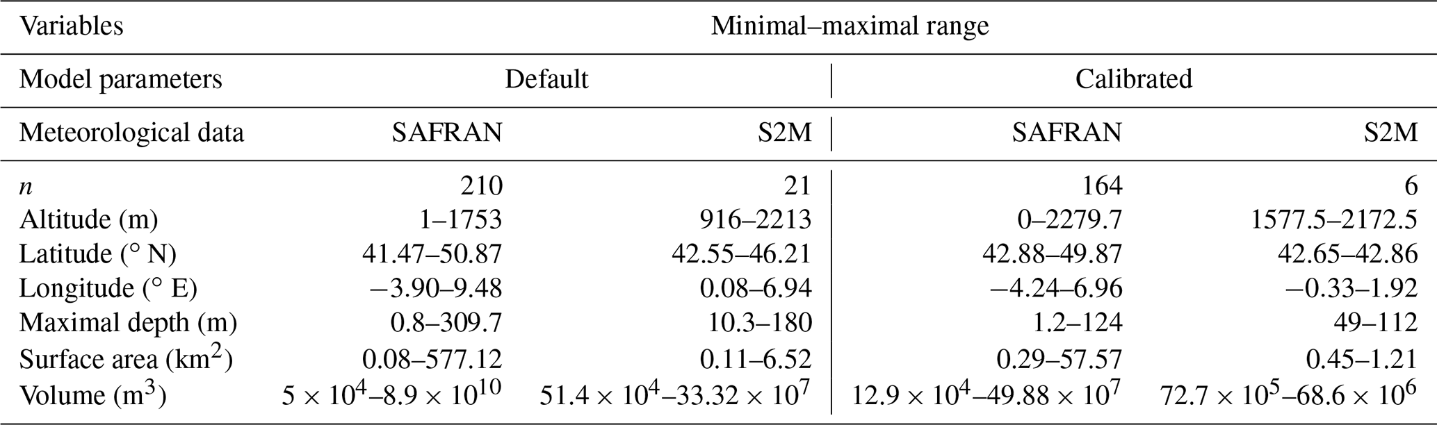
For this study, we considered 401 lakes (Fig. 1) located in Metropolitan France monitored according to the WFD. Here we refer to lakes as natural lakes, reservoirs, gravel pits and other artificial lakes (e.g., ponds and quarry lakes). The present lake dataset includes epilimnion and hypolimnion temperature simulations for 54 natural lakes, 302 reservoirs, 7 gravel pits and 38 other artificial lakes (Fig. 2). The lake characteristics range between 0 and 2279.7 m for altitude, between 0.8 and 309.7 m for maximal depth, between 0.08 and 577.12 km2 for surface area and between 5 × 10⁴ and 8.9 × 10¹⁰ m3 for volume.
The OKPLM was run for each lake using either default or calibrated parameters and either SAFRAN or S2M meteorological data. Specifically, calibrated model parameters were adopted when in situ temperature profiles along the water columns were available from the RCS/RCO monitoring network; these temperature profiles were then transformed and used as epilimnion and hypolimnion temperatures. For those lakes, calibration parameters (A, B, C, D, E, α and β) are lake-specific and determined using the lake-specific temperature profiles. Conversely, default parameters were used for the rest of the lakes as well as when bathymetry data necessary for the transformation of temperature profiles into epilimnion and hypolimnion temperatures were not available. In this case, the values of the parameters were estimated according to Eqs. (8) to (12).
SAFRAN data were used for most of the lakes, except for a few lakes at higher altitudes. Indeed, S2M data are more representative of mountainous meteorological conditions than SAFRAN data and were thus used, when possible, for simulating the water temperature in lakes situated at altitudes higher than 900 m. For some lakes, it was not possible to use S2M data, either because their drainage basins are not entirely part of a massif (n=1) or because they are located in massifs that are not covered by the S2M reanalysis dataset (n=18). Among the total number of study sites (n=401), the model was forced using SAFRAN and S2M meteorological data for 210 and 21 lakes with the default model parameters and for 164 and 6 lakes with calibrated model parameters. The geomorphological characteristics of the simulated lakes with each of the abovementioned configurations are shown in Table 1.
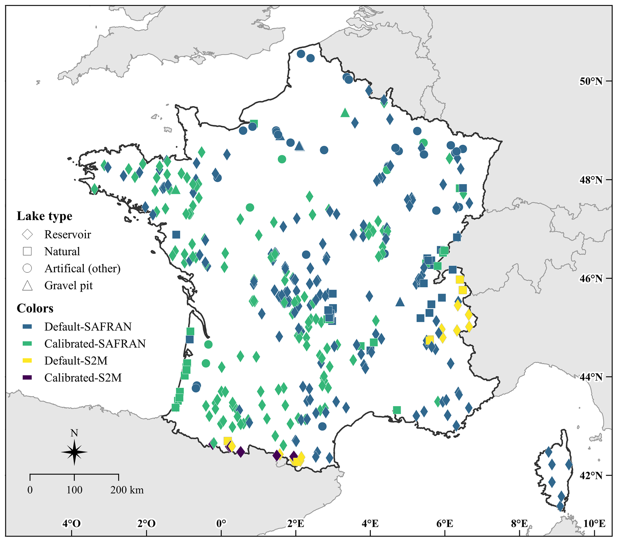
Figure 1Locations and lake types of the 401 French lakes simulated with the OKPLM in “default” and “calibrated” modes, with SAFRAN and S2M meteorological data for the period 1959–2020. The “other” artificial lakes consist of ponds and quarry lakes.
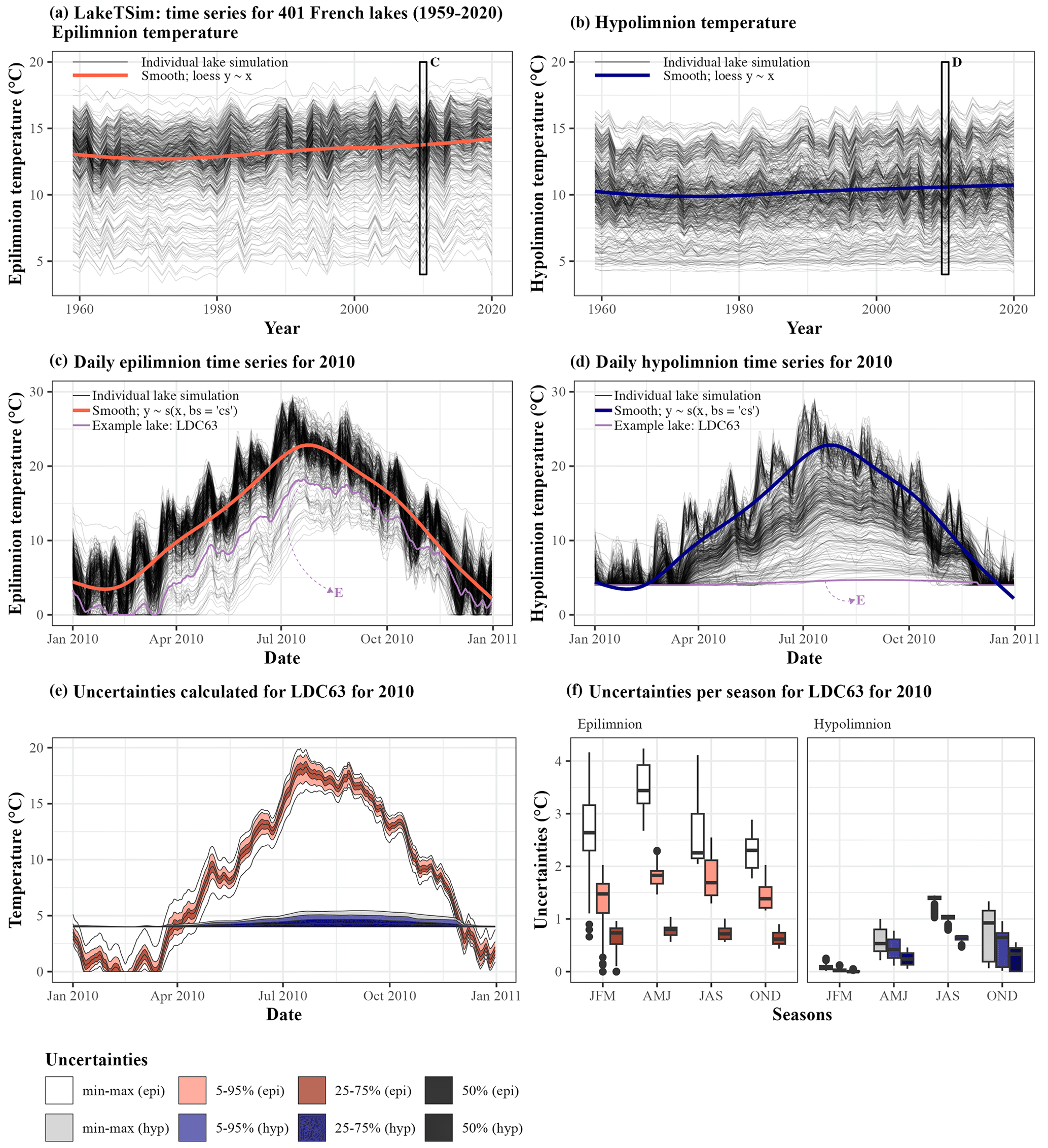
Figure 2Presentation of the LakeTSim data. (a) Epilimnion and (b) hypolimnion mean annual temperatures, with the average trend across the lakes shown with a smooth spline. (c) Daily epilimnion temperature per lake in the dataset for 2010, with a smooth spline and the time series for one lake (LDC63) highlighted. (d) Daily hypolimnion temperature per lake in the dataset for 2010, with a smooth spline and the time series for one lake (LDC63) highlighted. LDC63 is the code for Lake Chauvet, a natural lake (45.46∘ N, 2.83∘ E) located at 1167 m a.s.l., with a surface area of 0.51 km2, a volume of 17.41×10⁶ m3, and a maximum depth of 66.8 m. The simulation for LDC63 was conducted by resorting to SAFRAN data and was run with the calibrated mode. (e) Uncertainties were calculated per lake and per day and are shown here daily for LDC63, in 2010, for both the epilimnion (epi) and the hypolimnion (hyp). (f) Uncertainties are shown here seasonally for LDC63, in 2010, for both the epi and the hyp. JFM corresponds to January–February–March, AMJ corresponds to April–May–June, JAS corresponds to July–August–September, and OND corresponds to October–November–December.
Table 1Characteristics of the lakes simulated with the OKPLM in “default” and “calibrated” modes with SAFRAN and S2M meteorological data for the period 1959–2020; n represents the number of lakes.
2.5 Calibration, uncertainty and sensitivity analysis
Calibration, uncertainty and sensitivity analyses of model parameters were carried out using the CUSPY package, which is part of the ALAMODE software suite (Danis, 2020) and acts as an interface to the pyemu package (White et al., 2016, 2020). In addition to model parameters, sensitivity analysis was extended to encompass forcing parameters (MAAT, at_factor, sw_factor) as they provide information about the degree of sensitivity exhibited by model parameters in response to biases in the forcing data.
Parameter values were calibrated for lakes with available in situ data (temperature profiles and bathymetry). Parameter values were calibrated using the Gauss–Levenberg–Marquardt algorithm, the Tikhonov regularization (White et al., 2020) and the squared sum of residuals as an objective function. In addition to the calibrated parameter values, the calibration process also provided posterior parameter uncertainty and composite scaled sensitivities. Composite scaled sensitivities (CSSs) indicate the quantity of information provided by each parameter and the sensitivity of the model to them (Ely, 2006). The parameters with higher CSS values will have a greater impact on the resulting simulation compared to those with low CSS values. To determine the CSS values for each parameter, the dimensionless scaled sensitivities (DSSs) are used. DSSs indicate how important an observation or how sensitive a simulated equivalent of an observation is in relation to the estimation of a parameter. Further information on these statistical measures is available in Hill (1998) and Poeter and Hill (1997). The dimensionless scaled sensitivity for i and j, i being one of the observations and j being one of the parameters, is calculated as
where is the simulated value associated with the ith observation, bj is the jth estimated parameter, is the sensitivity of the simulated value associated with the ith observation and wi is the weight of the ith observation calculated based on the inverse of the variance–covariance matrix of the observation errors.
The CSS for parameter j is calculated from the DSS as follows:
where ND is the number of observations and b is a vector of parameter values.
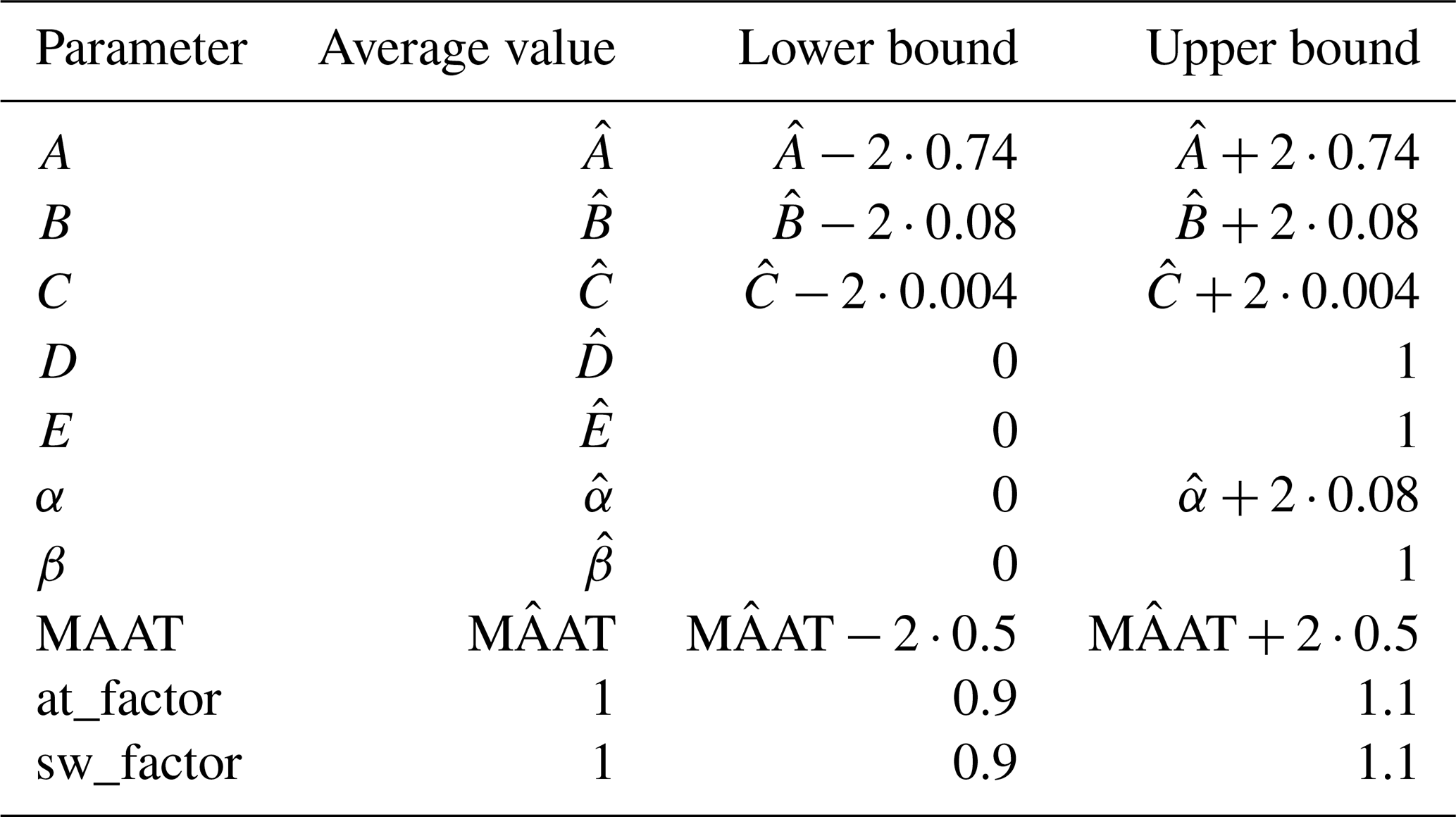
The uncertainty of the simulations (calibrated and default) was analyzed using Monte Carlo simulations. For each lake, 100 Monte Carlo simulations were carried by randomly selecting the values of the model parameters. Two parameters, at_factor and sw_factor, multiplying the meteorological input, were added to account for possible uncertainties in input data. For the default simulations, the a priori distribution of the parameters was assumed to follow a normal distribution with the average value and the lower and upper bounds shown in Table 2. The ranges for parameters A, B and C were estimated as 4 times the standard deviation of the residuals of the formulas used to estimate them according to Prats and Danis (2019). Parameters D, E and β are expected to lie in the range 0–1 for mathematical and physical reasons. However, their respective values are highly interdependent and are difficult to identify. Given their higher uncertainty, the full 0–1 range was explored. For MAAT, at_factor and sw_factor, reasonable ranges (±10 %) were chosen to account for meteorological data uncertainty (measurement error, errors in regionalization, etc.). For the calibrated simulations, the distribution of the parameters was obtained from the calibration results.
In this study, the non-parametric Kendall tau coefficient (significance level at 5 %) was used to identify statistical associations between uncertainty values and CSSs with respect to lake geomorphological characteristics (maximal depth, volume, surface area, latitude and altitude).
Table 2Characteristics of the a priori distributions of the model parameters. Parameters with a circumflex accent indicate parameter values estimated for a particular lake according to the regionalization formulas by Prats and Danis (2019).
The performance of the OKPLM was assessed in Prats and Danis (2019) by comparing its performance to two other often-applied models in lake studies, air2water (the four-parameter version) and FLake. The air2water model is a semi-empirical model used to calculate the epilimnion temperature of temperate lakes (Toffolon et al., 2014; Piccolroaz et al., 2013). FLake is a one-dimensional (1D) hydrodynamic lake model for simulating temperature vertical profiles and mixing conditions in lakes (Mironov, 2008). To assess their performances, the three models were run between 1999 and 2016 over two sets of French lakes of different types (reservoirs, natural lakes, ponds, quarry lakes and gravel pits): a group of 5 lakes with continuous profile measurements and a group of 404 lakes with less frequent temperature measurements. The performance assessment was limited to the period of 1999–2016 due to the availability of water temperature data (in situ and satellite) during that specific time frame. The scarcity of in situ water temperature measurements before 1999 applies to the entire set of lakes. However, it is important to note that long-term in situ water temperature data are available for a few large lakes and were used to assess the performance of the three models (Prats and Danis, 2015). The OKPLM was run with the default parameter values given by the parameterization in Prats and Danis (2019). The air2water parameter values were obtained as a function of lake depth from the parameterization presented in Toffolon et al. (2014) based on data from 14 lakes around the globe. In this case, the air2water model parameters were not calibrated due to the fact that the percentage of missing data within the LakeSST dataset employed in Prats and Danis (2019) exceeded 97 % for most lakes. Beyond this threshold of 97 % missing data, the performance of the calibrated four-parameter version of the air2water model was found to be unsatisfactory (Piccolroaz, 2016). However, when evaluating the model performance with the set of five lakes with continuous data, air2water was run using parameter values calibrated for the individual lakes' available data. FLake does not have calibration parameters. Meteorological forcing (SAFRAN) consisted of air temperature for the air2water model; solar radiation, vapor pressure, cloud cover and wind speed for FLake; and air temperature and solar radiation for the OKPLM.
The OKPLM, air2water and FLake simulations were assessed through comparison to in situ measurements. For epilimnion temperatures, the average discrepancies calculated between OKPLM simulations and observations remained below 2 ∘C in most cases, in contrast to the air2water and FLake models. The performance comparison between the OKPLM, air2water and FLake yielded median RMSEs (root mean square errors) of 1.7, 2.3 and 2.6 ∘C, respectively, calculated between simulations and observations of the epilimnion water temperature, although, when using calibrated parameter values for air2water, the median RMSE was below 1 ∘C in most cases. For hypolimnion temperatures, the median RMSEs by lake type obtained with OKPLM simulations remained below 2 ∘C, except for gravel pits (RMSE = 2.7 ∘C) and reservoirs (RMSE = 2.3 ∘C), whereas FLake yielded a median RMSE of 3.3 ∘C. For the epilimnion temperatures, the differences between the RMSEs of lake types were not significant. In terms of depth, discrepancies between epilimnion temperature simulations with the OKPLM and measurements were highest for lakes with a depth >10 m and for ponds around 1 m deep. The OKPLM simulations were also evaluated seasonally, in particular during summer and winter. The model simulated temperatures well, with median RMSEs of 1.4 and 1.6 ∘C in summer and winter, respectively.
Overall, for both simulations with default and calibrated model parameters, uncertainty was higher for hypolimnion temperature compared to epilimnion temperature, especially in reservoirs (Fig. 3). In the default simulations, the uncertainty of the simulated epilimnion temperatures showed a clear and strong relation to lake maximal depth (Fig. 3, Table 3). On the one hand, the maximal depth had the highest Kendall tau value of 0.64 (p value <0.0001), indicating a strong positive correlation with uncertainty, followed by volume with a Kendall tau of 0.59 (p value <0.0001). Uncertainty increased with maximal depth and volume, in particular for lakes with depths greater than 10 m and volumes greater than 106 m3 (Fig. 3). Overall, lakes with higher maximal depths have higher volumes and are located at greater altitudes (Figs. A1–A2 in Appendix A). On the other hand, moderate significant correlations were identified with surface area, altitude and latitude (Table 3). Lakes with larger surface areas and higher altitudes tend to have higher uncertainties, whereas lakes located at higher latitudes tend to have lower uncertainties (Fig. A3 in Appendix A). The latter can be linked to the fact that more shallow lakes are located at higher latitudes (Fig. A1 in Appendix A). For default simulations of hypolimnion temperatures, uncertainty was maximal for lakes with depths around 10 m. Kendall's tau values revealed a moderate significant correlation between hypolimnion temperature uncertainty and altitude (−0.45, p value <0.0001). The decrease in uncertainties with altitude can be related to the fact that lakes situated at very high altitudes are mostly deep. Further, in the present dataset, lakes with higher maximal depths occur as altitude increases (Figs. A1–A2 in Appendix A).
After calibration, there was an important reduction in simulation uncertainty. For default simulations of epilimnion temperature, the median of the 90 % confidence uncertainty range was 5.42 ∘C, while after calibration it was 1.85 ∘C. For hypolimnion temperature, the median of the 90 % confidence uncertainty range of the default simulations was 8.5 ∘C, while it was 2.32 ∘C after calibration. However, many reservoirs with depths greater than 8 m still had a much greater uncertainty (uncertainty range >4 ∘C) than the rest of the lakes after calibration. Additionally, reservoirs (and a few natural lakes) above 100 m in altitude showed the highest uncertainties in the simulation of epilimnion temperature.
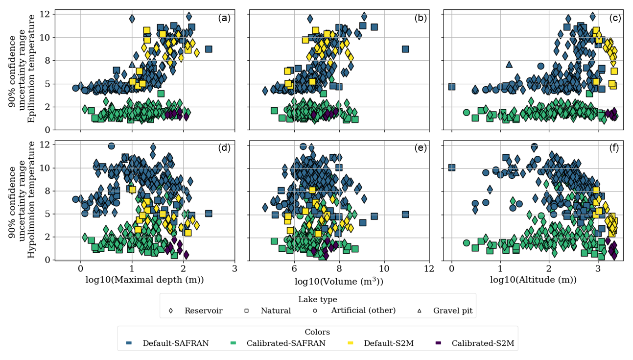
Figure 3Average 90 % confidence uncertainty range for epilimnion (a–c) and hypolimnion (d–f) temperatures in calibrated (n=170) and default (n=231) simulations for the period 1959–2020. The other artificial lakes consist of ponds and quarry lakes.
Table 3Kendall's tau coefficients and p values of the average 90 % confidence uncertainty range for epilimnion and hypolimnion temperatures obtained from default simulations (1959–2020) with respect to lake geomorphological characteristics. For each lake, “epilimnion uncertainty” and “hypolimnion uncertainty” are defined as the average 90 % confidence uncertainty range calculated as the difference between the 95th and 5th percentiles of the daily simulated epilimnion and hypolimnion water temperatures.
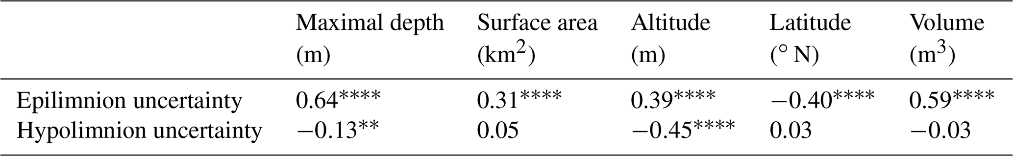
The significance levels are represented as follows. *: value ; : value ; : value ; : p value . Otherwise, correlations are not significant (p value >0.05).
The parameter to which the model was most sensitive was parameter C (Fig. 4), which multiplies solar radiation in Eq. (1). The CSSs for C were 1 order of magnitude greater than for the next parameters with the highest CSSs, parameters α and at_factor, both influencing the effect of air temperature on simulated water temperature. Other parameters to which the model was somewhat sensitive were E, B and β. The model was quite insensitive to sw_factor, MAAT and A. Parameter D, with CSSs several orders of magnitude smaller than the other parameters, was unidentifiable.
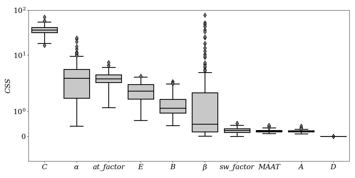
Figure 4Composite scaled sensitivities (CSSs) for each parameter. The boxplots indicate the distribution of CSSs between the simulations calibrated for different lakes. The y axis is in logarithmic form.
The model tended to be more sensitive to the parameter values in the case of reservoirs than in the case of natural lakes (Figs. 5 and A4–A7 in Appendix A). Some parameters showed a dependency on lake geomorphological characteristics. With the exception of a weak correlation with altitude (Kendall's tau = 0.18), there was no significant dependence between parameter C and lake geomorphological characteristics (Table 4 and Fig. A4 in Appendix A). Parameter α being parameterized as a function of lake volume, surface area and altitude reflect the thermal inertia of the lake. This showed a clear, highly significant dependency, primarily on lake depth (Kendall's tau = 0.47) and followed by altitude (Kendall's tau = 0.4) and volume (Kendall's tau = 0.39) (Fig. 5, Table 4). The increase in model sensitivity to parameter α, primarily with depth as well as altitude and volume, propagated to the default simulations and explains the increased uncertainty with these same geomorphological characteristics in the default simulations. The parameter at_factor was weakly but significantly correlated with all lake geomorphological characteristics except for latitude, with which no correlation was found (Fig. 5, Table 4 and Figs. A4–A7 in Appendix A). CSSs were mostly low for parameter β, except for a few reservoirs and artificial lakes that scored very high CSS values. The sensitivity of β displayed a weak but significant correlation with lake geomorphological characteristics, except for volume (Table 4).
Although the model in general was not very sensitive to the values of the parameters most directly related to hypolimnion temperatures (D, E, β), the quality of hypolimnion temperatures was greatly improved through calibration. This would seem to indicate that the quality of the simulated hypolimnion temperature was improved through the improvement of epilimnion temperature simulations.
Table 4Kendall's tau coefficients and p values of CSSs for model parameter values and drivers obtained from calibrated simulations (1959–2020) with respect to lake geomorphological characteristics.
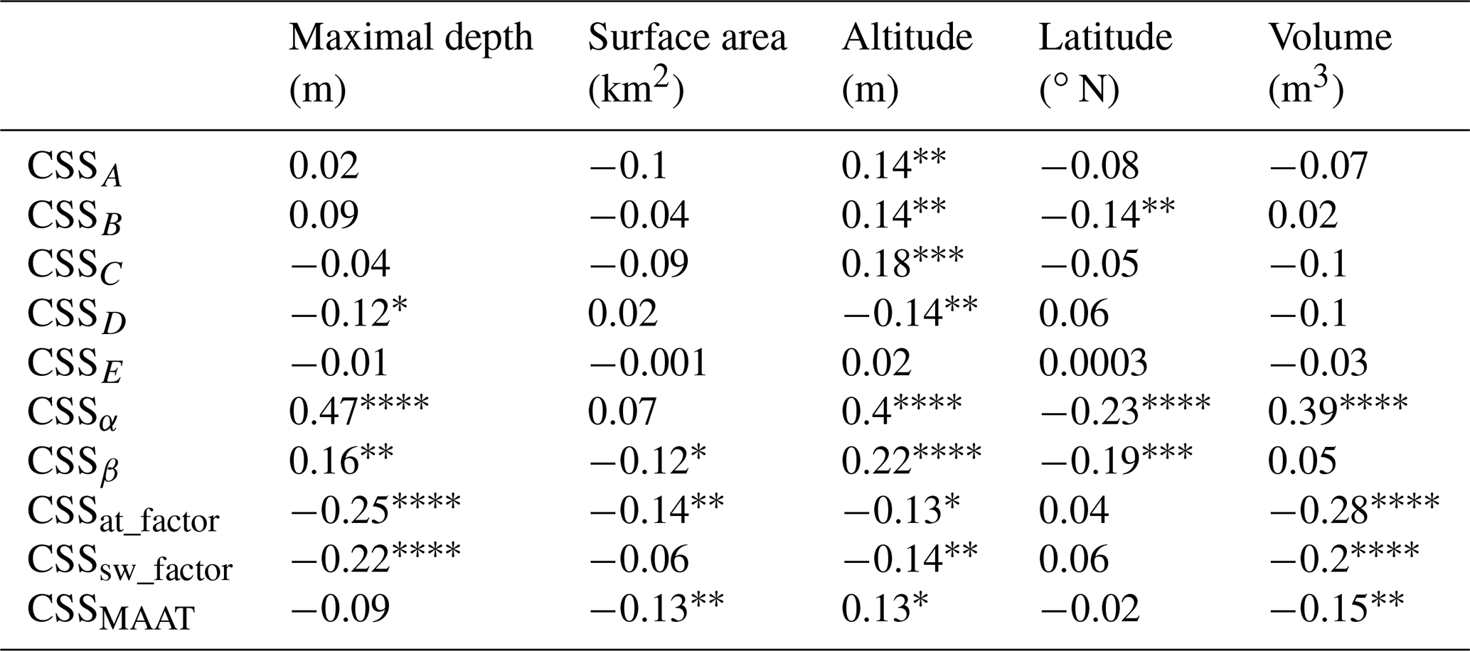
The significance levels are represented as follows. *: value ; : value ; : value ; : p value . Otherwise, correlations are not significant (p value >0.05).
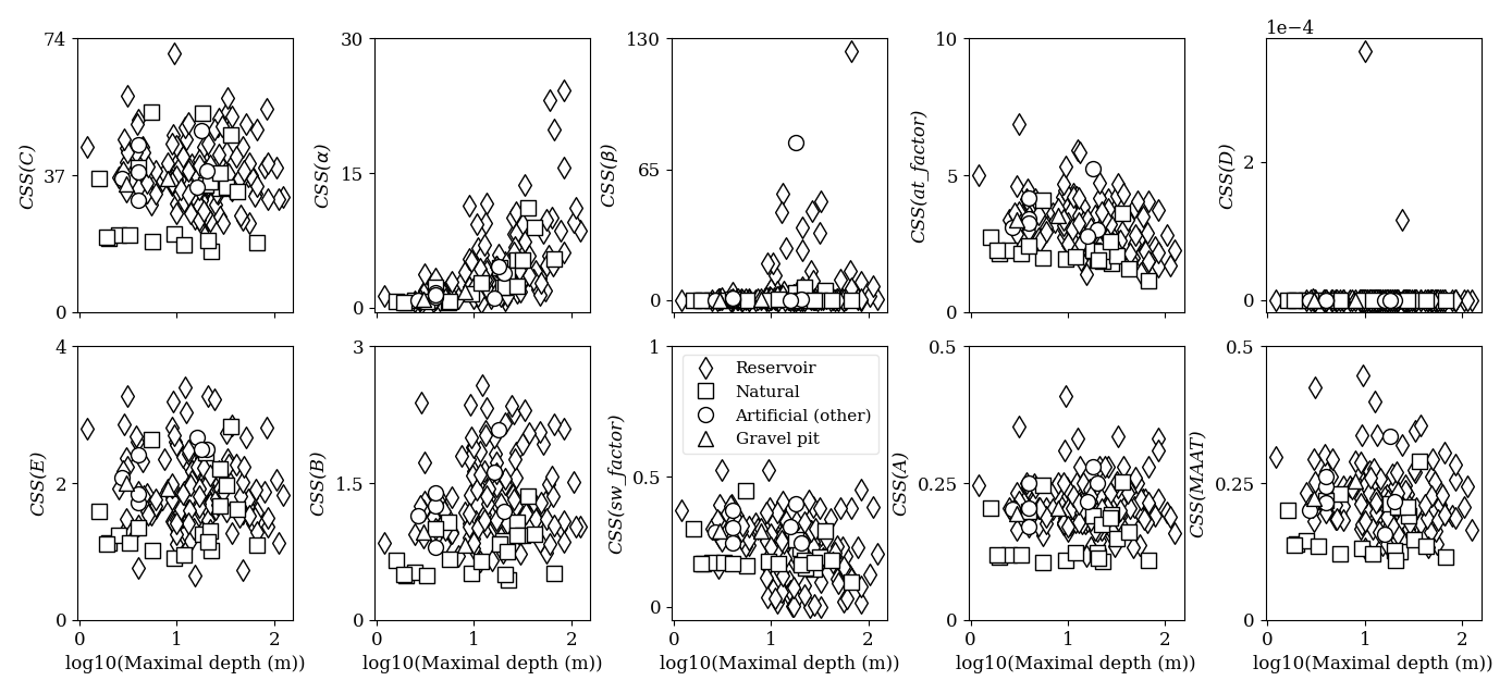
Figure 5CSSs for each model parameter as a function of maximal depth. The other artificial lakes consist of ponds and quarry lakes.
Lakes are undeniably changing under climate change, and long-term future projections show that the shifts in ecosystem functioning will continue with aggravated alterations (Woolway and Merchant, 2019). In particular, given the key role of lake water temperature in regulating ecosystem processes, its warming has become a response that is crucial to monitor, explore and understand. Hence, the importance of developing or adopting approaches, such as numerical models, will provide long-term information about water temperature and allow us to understand the thermal response of lakes to climate change.
Here we used a semi-empirical model, the OKPLM, to simulate 6 decades of epilimnion and hypolimnion water temperatures in French lakes. In comparison to similar models, overall, the OKPLM provides acceptable estimations of water temperatures, with better results for epilimnion temperatures. The values of the RMSEs provided in Prats and Danis (2019) and obtained between OKPLM simulations and observations are comparable to values found in studies applying complex hydrodynamic lake models (Read et al., 2014; Fang et al., 2012). When using the default parameter values, the uncertainty associated with epilimnion temperature simulations was significantly related to all geomorphological characteristics; however, it was especially strongly correlated with lake maximal depth. In contrast, the uncertainty in the hypolimnion simulations had a significant correlation solely with altitude and maximal depth. The importance of this correlation was especially noteworthy in the case of reservoirs located in low-altitude regions where uncertainties were lowest. While the association between hypolimnion uncertainty and maximal depth exhibited only a weak correlation, the instances of the highest uncertainties were predominantly found in reservoirs with maximal depths around 10 m. The correlations found between lake geomorphological characteristics and simulation uncertainties suggest that there might be systematic biases in the definition of model parameters or in the forcing data. The calibration of model parameters significantly reduced the uncertainties, yet, for hypolimnion temperatures, they remained considerably high and increased with depth, especially in reservoirs.
The high levels of uncertainty found in reservoirs could be somewhat attributed to the lack of consideration of water level fluctuations in the model. In contrast to other lakes (e.g., natural lakes, artificial lakes and gravel pits), reservoirs experience significant variations in their water level, which influences the heat budget and hence their thermal regime. Therefore, even under similar meteorological conditions, lakes and reservoirs could have different thermal behaviors (Nowlin et al., 2004). In reservoirs, the discharge depth is a driver of thermal structure. Deep discharges could contribute to warmer bottom waters (Carr et al., 2020), whereas, in some cases, if the reservoir is shallow or if the discharge depth is not deep, it could demonstrate lake-like thermal behavior. This does not necessarily mean that, in this case, the entire functioning of the reservoir resembles one of a natural lake; there are still differences to consider (Detmer et al., 2021).
The application of the OKPLM should be done with caution given its performance and depending on the objective of the study. The model does not take into account a complete set of meteorological forcing (e.g., with cloud cover, relative humidity and wind speed and direction) or other variables (e.g., inflow and outflow rates or water level fluctuations, inflow discharge depth and inflow temperature) that could influence the thermal structure of the ecosystem (Yang et al., 2020; Carr et al., 2020). Furthermore, the OKPLM was parameterized for a specific set of lakes with particular geomorphological characteristics. Thus, it would be advisable to apply the model over lakes with similar characteristics. If the aim is to conduct a long-term regional or global study for studying general patterns of climate change impacts over a large number of study sites, the utilization of semi-empirical models such as the OKPLM is the most suitable choice. Although complex, deterministic or process-based models provide more accurate representations of thermal conditions, applying these models over several study sites and for long periods is usually hindered by the scarcity of the required input data. The increased complexity of these models (with reference to an increased number of model parameters) is beneficial for representing additional ecosystem processes. However, the greater number of model parameters increases the sensitivity of models and requires more calibration efforts (Lindenschmidt, 2006). Furthermore, a reduction in model errors is sometimes associated with an increased complexity in model structure; however, this is not always consistent, since a complex model does not necessarily provide better estimations and thus lower errors than a simple model (Snowling and Kramer, 2001).
Our goal in publishing the present dataset is to expand knowledge about the water temperature of French lakes and to provide data with enough details and reliability so that it could be implemented in different studies where water temperature is used to understand specific processes or interactions, in particular under climate change, hence the significance of the present findings. The present study, making use of a semi-empirical model to provide long-term data on water temperature, was necessary for several reasons. Equipping a large number of lakes with thermal sensors is challenging and labor-intensive: it comes with a high financial cost that is often not available. Consequently, historical and even current water temperature datasets are often scarce, which can be problematic for studying the impact of climate change, as it requires high-frequency data over a long duration of time for accurate analysis. In general, the higher the sampling frequency and duration, the better the data are suited to estimating or analyzing specific processes or warming trends. The sampling frequency and length of a dataset have been shown to play a role in determining the accuracy of estimating warming trends where time series longer than 30 years seem to be the most appropriate ones (Gray et al., 2018). Although the duration and frequency of a dataset have a major role in reflecting accurate representations, their influence is scarcely addressed when it comes to climate change studies related to warming trends in water temperature.
This dataset will be useful for climate change studies; it could be used to develop and analyze several temperature indicators (e.g., annual or seasonal maximal and minimal temperature values, temperature exceeding certain thresholds with biological implications). Further, mixing and stratification dynamics are important to characterize as they drive lake biogeochemistry. Among other processes, they influence the distribution of nutrients, primary productivity and the composition of phytoplankton and zooplankton communities along the water column (Judd et al., 2005). With the LakeTSim dataset, it is possible to classify the mixing regime of lakes and to investigate possible triggers of regime shifts.
The LakeTSim dataset comprises water temperature simulations for natural lakes (n=54), reservoirs (n=302), gravel pits (n=7) and other artificial lakes (e.g., ponds and quarry lakes, n=38). The simulations are for both the epilimnion and hypolimnion. Lakes that are fully mixed throughout the year (typically shallower lakes) have the same temperature value for both layers. More generally, the delta of temperature can be used to calculate mixing regimes (Sharaf et al., in preparation).
The lakes in the dataset were selected because they are monitored as part of the European Water Framework Directive (Directive 2000/60/EC). The majority of the 401 lakes are non-natural, and some were only created after 1959 (i.e., the start of our simulations). We compiled the initial temporal gap filling related to the initial filling years for 282 of these 347 non-natural lakes (269 reservoirs and 13 artificial lakes, Fig. A8 in Appendix A) in Table S1 (see the Supplement) to be used as a companion dataset to LakeTSim. The filling years were sourced from https://www.barrages-cfbr.eu (last access: 27 April 2023) for 179 of the lakes and from the PLAN_DEAU database for 103 of the lakes; the information was not available for 33 reservoirs, 7 gravel pits and 25 other artificial lakes of the LakeTSim dataset.
The median filling date was 1962, and 67 % of the lakes with known filling dates were filled by 1980. While the complete simulations ranging from 1959 to 2020 can also be used as a theoretical lake temperature for comparison across similar periods, we recommend that users of LakeTSim data for reservoir and artificial lake simulations consider the initial filling dates provided in Table S1 to filter out years from the simulations during which lakes were not filled yet.
Additionally, users should be aware that some reservoirs might be drained completely at certain intervals (e.g., every 10 years) for maintenance and inspection purposes and that this is not reflected in our dataset. Finally, as mentioned in the discussion, some of the lakes in the dataset experience artificial (e.g., in reservoirs) or natural (e.g., in some smaller ponds) water level fluctuations and potential intermittent dry periods lasting weeks or months; none of these hydrological processes is accounted for in the simulations.
The LakeTSim dataset (Sharaf et al., 2023) for the epilimnion and hypolimnion water temperature simulations and the supporting information are available at https://doi.org/10.57745/OF9WXR. The “00_Data_description.txt” file contains a description of the dataset. The geographical (longitude and latitude) and morphological (surface area, volume and maximal depth) data for the 401 lakes are presented in the “01_Lake_data.txt” file in addition to the name, type, altitude and identification code for each lake. The data are located in two main folders: “02_Temperature_data” containing daily epilimnion (tepi) and hypolimnion (thyp) temperatures simulated with the OKPLM as well as “03_Uncertainty_ data” containing daily tepi and thyp uncertainties. In each folder, the data for temperature simulations and their uncertainties are presented in text files available in the “00_LakeTSim_SAFRAN_OKPdefault_data”, “01_LakeTSim_SAFRAN_OKPcalibrated_data”, “02_LakeTSim_S2M_OKPdefault_data” and “03_LakeTSim_S2M_OKPcalibrated_data” folders. The name of each file within these folders includes the identification code of the lake. The uncertainty data are visible for each lake in the geoportal at http://geo.ecla.inrae.fr/maps (last access: 2 December 2023).
The respective codes for the CUSPY (https://doi.org/10.5281/zenodo.7585606, Prats-Rodríguez and Danis, 2023a) and OKPLM (https://doi.org/10.5281/zenodo.7585615, Prats-Rodríguez and Danis, 2023b) packages, which can be used to conduct sensitivity and uncertainty analyses and to run the OKPLM, are available at https://github.com/inrae/ALAMODE-cuspy (last access: 27 November 2023) and https://github.com/inrae/ALAMODE-okp (last access: 27 November 2023) as well as ZENODO.
We present the LakeTSim dataset and the semi-empirical OKPLM for simulating water temperature in lakes. We applied the model over a set of 401 French lakes for the period 1959–2020 to derive daily simulations of epilimnion and hypolimnion water temperatures, here referred to as the LakeTSim dataset. Previous efforts to assess the model's performance show an overall acceptable representation of epilimnion and hypolimnion temperatures when compared to in situ measurements. The uncertainty analysis of the simulations demonstrates that higher uncertainties are found for, by order of relative importance, (1) default simulations, (2) hypolimnion compared to epilimnion temperatures and (3) deep lakes, in particular reservoirs (maximal depths greater than 10 m for epilimnion temperature and around 10 m for hypolimnion temperature simulated with the default model parameters). Although the calibration significantly decreases the uncertainties related to both the epilimnion and hypolimnion, in some cases they are still considerable in the hypolimnion. Based on these results and whether enough observation data are available, optimally we recommend the use of the OKPLM for shallow (maximal depth <8 m) lakes with calibrated model parameters. However, when applied in its default or even calibrated configuration over deep lakes, one should be aware of the presented limitations and address them in the analysis. The LakeTSim dataset is valuable for assessing the impact of climate change on the thermal functioning of lakes, which is often hindered by the lack of water temperature observations. The present dataset will provide new insights into the thermal behavior of French lakes, which can provide a useful context for stakeholders as they design management strategies in the context of climate change.
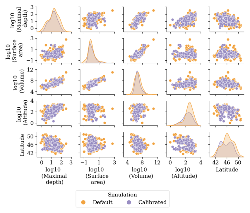
Figure A1Scatter plots of lake (n=401) geomorphological characteristics: maximal depth (m), surface area (km2), volume (m3), altitude (m) and latitude (∘ N).
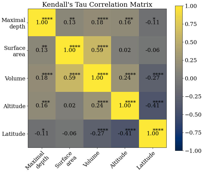
Figure A2Kendall's tau correlation matrix of the geomorphological characteristics of lakes simulated in “default” mode (n=231): maximal depth (m), surface area (km2), volume (m3), altitude (m) and latitude (∘ N). The significance levels are represented as follows. *: value ; : value ; : value ; : p value . Otherwise, correlations are not significant (p value >0.05).
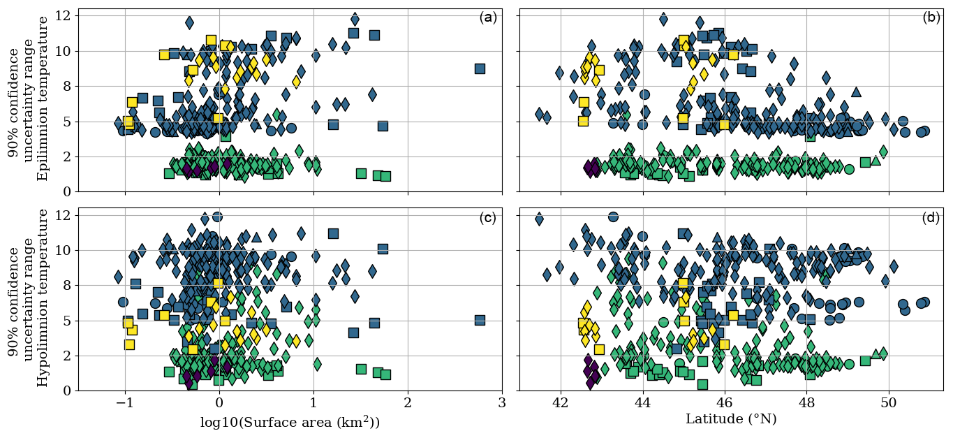
Figure A3Average 90 % confidence uncertainty range for epilimnion (a, b) and hypolimnion (c, d) temperatures in calibrated (n=170) and default (n=231) simulations for the period 1959–2020 as a function of surface area (km2) and latitude (∘ N). The “other” artificial lakes consist of ponds and quarry lakes.

Figure A4CSSs for each model parameter as a function of altitude. The other artificial lakes consist of ponds and quarry lakes.
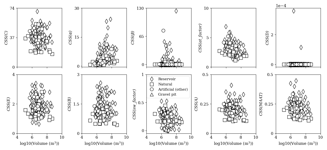
Figure A5CSSs for each model parameter as a function of volume. The other artificial lakes consist of ponds and quarry lakes.
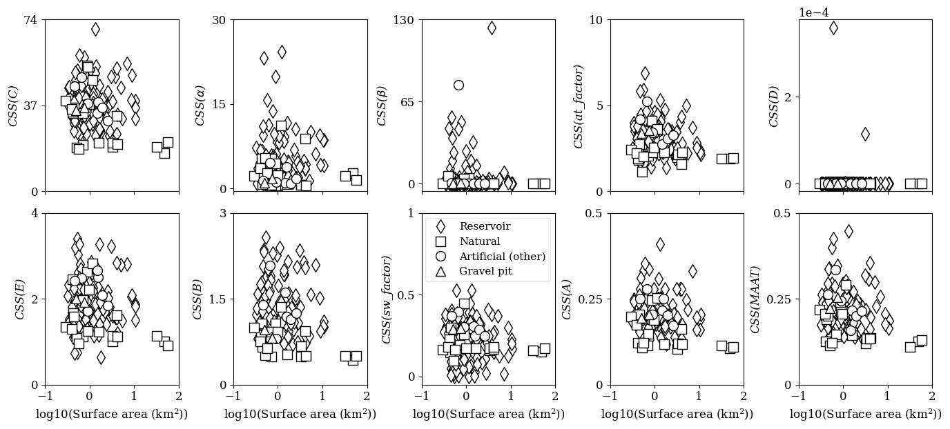
Figure A6CSSs for each model parameter as a function of surface area. The other artificial lakes consist of ponds and quarry lakes.
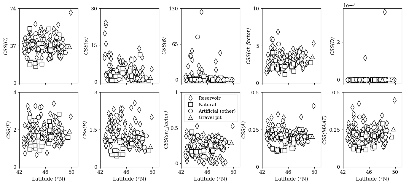
Figure A7CSSs for each model parameter as a function of latitude. The other artificial lakes consist of ponds and quarry lakes.
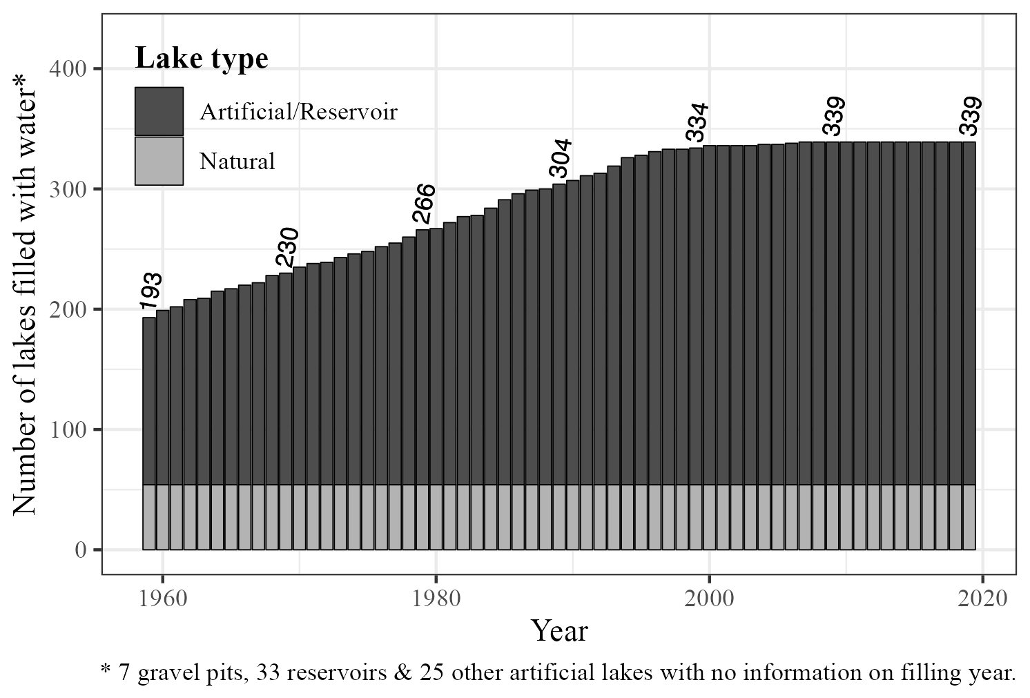
Figure A8Distribution of initial filling years for lakes (e.g., reservoirs, gravel pits, ponds and quarry lakes) of the LakeTSim dataset.
The supplement related to this article is available online at: https://doi.org/10.5194/essd-15-5631-2023-supplement.
NS wrote the original manuscript with input from JP and PAD. NS, JP and PAD discussed the results. JP developed and carried out the implementation of the OKPLM and the uncertainty computation in ALAMODE. JP and NS performed the simulations and provided uncertainty analysis results with SAFRAN and S2M data, respectively. JP and NS implemented the integration of SAFRAN and S2M data, respectively, in ALAMODE. NS prepared the LakeTSim dataset. JP and NS provided the uncertainty and sensitivity analysis. PAD designed, contributed and supervised the implementation of S2M data in ALAMODE for forcing the OKPLM when simulating high-altitude lakes. PAD supervised the findings of this work. RB proposed and contributed to the integration of the data consisting of initial filling dates of reservoirs and other artificial lakes in the paper. NR and TT supervised and contributed to the implementation of simulation results in the database. NR processed S2M data and compiled the data for the initial filling years of the reservoirs and other artificial lakes. NS, RB and NR prepared the figures. NR and TT prepared the DOI for the LakeTSim dataset. TP conducted the fieldwork for the monitoring, acquisition and verification of in situ temperature data. All the authors reviewed, edited and approved the final paper.
The contact author has declared that none of the authors has any competing interests.
Publisher's note: Copernicus Publications remains neutral with regard to jurisdictional claims made in the text, published maps, institutional affiliations, or any other geographical representation in this paper. While Copernicus Publications makes every effort to include appropriate place names, the final responsibility lies with the authors.
The authors thank Météo-France for providing SAFRAN and S2M meteorological data, Matthieu Vernay for his feedback on the utilization of S2M data and the Réseau Lacs Sentinelles for providing bathymetry data for mountain lakes.
The authors received funding from the OFB (Office Français de la Biodiversité), SEGULA Technologies, INRAE (Institut National de Recherche pour l'Agriculture, l'Alimentation et l'environnement) and Pôle R&D ECLA (ECosystèmes LAcustres).
This paper was edited by Christof Lorenz and reviewed by two anonymous referees.
Adrian, R., O'Reilly, C. M., Zagarese, H., Baines, S. B., Hessen, D. O., Keller, W., Livingstone, D. M., Sommaruga, R., Straile, D., Van Donk, E., Weyhenmeyer, G. A., and Winder, M.: Lakes as sentinels of climate change, Limnol. Oceanogr., 54, 2283–2297, https://doi.org/10.4319/lo.2009.54.6_part_2.2283, 2009.
Allan, M. G., Hamilton, D. P., Trolle, D., Muraoka, K., and McBride, C.: Spatial heterogeneity in geothermally-influenced lakes derived from atmospherically corrected Landsat thermal imagery and three-dimensional hydrodynamic modelling, Int. J. Appl. Earth Obs. Geoinf., 50, 106–116, https://doi.org/10.1016/j.jag.2016.03.006, 2016.
Babbar-Sebens, M., Li, L., Song, K., and Xie, S.: On the Use of Landsat-5 TM Satellite for Assimilating Water Temperature Observations in 3D Hydrodynamic Model of Small Inland Reservoir in Midwestern US, Adv. Remote Sens., 2, 214–227, https://doi.org/10.4236/ars.2013.23024, 2013.
Carr, M. K., Sadeghian, A., Lindenschmidt, K. E., Rinke, K., and Morales-Marin, L.: Impacts of Varying Dam Outflow Elevations on Water Temperature, Dissolved Oxygen, and Nutrient Distributions in a Large Prairie Reservoir, Environ. Eng. Sci., 37, 78–97, https://doi.org/10.1089/ees.2019.0146, 2020.
Danis, P.-A.: Rapport d'avancement sur les outils de modélisation thermique, [Rapport Technique], OFB, INRAE, Université Savoie Mont Blanc, 1–8, https://hal.inrae.fr/hal-03253847 (last access: 4 December 2023), 2020.
Daufresne, M., Lengfellner, K., and Sommer, U.: Global warming benefits the small in aquatic ecosystems, P. Natl. Acad. Sci. USA, 106, 12788–12793, https://doi.org/10.1073/pnas.0902080106, 2009.
Detmer, T. M., Parkos, J. J., and Wahl, D. H.: Long-term data show effects of atmospheric temperature anomaly and reservoir size on water temperature, thermal structure, and dissolved oxygen, Aquat. Sci., 84, 3, https://doi.org/10.1007/s00027-021-00835-2, 2021.
Durand, Y., Brun, E., Merindol, L., Guyomarc'h, G., Lesaffre, B., and Martin, E.: A meteorological estimation of relevant parameters for snow models, Ann. Glaciol., 18, 65–71, https://doi.org/10.3189/S0260305500011277, 1993.
Ely, D. M.: Analysis of sensitivity of simulated recharge to selected parameters for seven watersheds modeled using the precipitation-runoff modeling system, Scientific Investigations Report, 26 pp., https://doi.org/10.3133/sir20065041, 2006.
Fang, X., Alam, S. R., Stefan, H. G., Jiang, L., Jacobson, P. C., and Pereira, D. L.: Simulations of water quality and oxythermal cisco habitat in Minnesota lakes under past and future climate scenarios, Water Qual. Res. J. Canada, 47, 375–388, https://doi.org/10.2166/wqrjc.2012.031, 2012.
Gray, D. K., Hampton, S. E., O'Reilly, C. M., Sharma, S., and Cohen, R. S.: How do data collection and processing methods impact the accuracy of long-term trend estimation in lake surface-water temperatures?, Limnol. Oceanogr. Methods, 16, 504–515, https://doi.org/10.1002/lom3.10262, 2018.
Griffith, A. W. and Gobler, C. J.: Harmful algal blooms: A climate change co-stressor in marine and freshwater ecosystems, Harmful Algae, 91, 101590, https://doi.org/10.1016/j.hal.2019.03.008, 2020.
Halverson, G. H., Lee, C. M., Hestir, E. L., Hulley, G. C., Cawse-Nicholson, K., Hook, S. J., Bergamaschi, B. A., Acuña, S., Tufillaro, N. B., Radocinski, R. G., Rivera, G., and Sommer, T. R.: Decline in Thermal Habitat Conditions for the Endangered Delta Smelt as Seen from Landsat Satellites (1985–2019), Environ. Sci. Technol., 56, 185–193, https://doi.org/10.1021/acs.est.1c02837, 2022.
Havens, K. and Jeppesen, E.: Ecological responses of lakes to climate change, Water, 10, 917, https://doi.org/10.3390/w10070917, 2018.
Hill, M. C.: Methods and guidelines for effective model calibration: U.S. Geological Survey Water-Resources Investigations Report 98-4005, 90 pp., https://doi.org/10.3133/wri984005, 1998.
Hipsey, M. R., Bruce, L. C., Boon, C., Busch, B., Carey, C. C., Hamilton, D. P., Hanson, P. C., Read, J. S., de Sousa, E., Weber, M., and Winslow, L. A.: A General Lake Model (GLM 3.0) for linking with high-frequency sensor data from the Global Lake Ecological Observatory Network (GLEON), Geosci. Model Dev., 12, 473–523, https://doi.org/10.5194/gmd-12-473-2019, 2019.
Janssen, A. B. G., Hilt, S., Kosten, S., de Klein, J. J. M., Paerl, H. W., and Van de Waal, D. B.: Shifting states, shifting services: Linking regime shifts to changes in ecosystem services of shallow lakes, Freshw. Biol., 66, 1–12, https://doi.org/10.1111/fwb.13582, 2021.
Javaheri, A., Babbar-Sebens, M., and Miller, R. N.: From skin to bulk: An adjustment technique for assimilation of satellite-derived temperature observations in numerical models of small inland water bodies, Adv. Water Resour., 92, 284–298, https://doi.org/10.1016/j.advwatres.2016.03.012, 2016.
Judd, K. E., Adams, H. E., Bosch, N. S., Kostrzewski, J. M., Scott, C. E., Schultz, B. M., Wang, D. H., and Kling, G. W.: A case history: Effects of mixing regime on nutrient dynamics and community structure in third sister lake, michigan during late winter and early spring 2003, Lake Reserv. Manag., 21, 316–329, https://doi.org/10.1080/07438140509354437, 2005.
Kettle, H., Thompson, R., Anderson, N. J., and Livingstone, D. M.: Empirical modeling of summer lake surface temperatures in southwest Greenland, Limnol. Oceanogr., 49, 271–282, https://doi.org/10.4319/lo.2004.49.1.0271, 2004.
Kharouba, H. M., Ehrlén, J., Gelman, A., Bolmgren, K., Allen, J. M., Travers, S. E., and Wolkovich, E. M.: Global shifts in the phenological synchrony of species interactions over recent decades, P. Natl. Acad. Sci. USA, 115, 5211–5216, https://doi.org/10.1073/pnas.1714511115, 2018.
Kim, J., Seo, D., Jang, M., and Kim, J.: Augmentation of limited input data using an artificial neural network method to improve the accuracy of water quality modeling in a large lake, J. Hydrol., 602, 126817, https://doi.org/10.1016/j.jhydrol.2021.126817, 2021.
Layden, A., Merchant, C., and Maccallum, S.: Global climatology of surface water temperatures of large lakes by remote sensing, Int. J. Climatol., 35, 4464–4479, https://doi.org/10.1002/joc.4299, 2015.
Lind, L., Eckstein, R. L., and Relyea, R. A.: Direct and indirect effects of climate change on distribution and community composition of macrophytes in lentic systems, Biol. Rev., 1686, 1677–1690, https://doi.org/10.1111/brv.12858, 2022.
Lindenschmidt, K. E.: The effect of complexity on parameter sensitivity and model uncertainty in river water quality modelling, Ecol. Modell., 190, 72–86, https://doi.org/10.1016/j.ecolmodel.2005.04.016, 2006.
Mironov, D. V.: Parameterization of lakes in numerical weather prediction: Description of a lake model, COSMO Technical Report No. 11, Deutscher Wetterdienst, https://api.semanticscholar.org/CorpusID:54696443 (last access: 4 December 2023), 2008.
Nouchi, V., Kutser, T., Wüest, A., Müller, B., Odermatt, D., Baracchini, T., and Bouffard, D.: Resolving biogeochemical processes in lakes using remote sensing, Aquat. Sci., 81, 27, https://doi.org/10.1007/s00027-019-0626-3, 2019.
Nowlin, W. H., Davies, J. M., Nordin, R. N., and Mazumder, A.: Effects of water level fluctuation and short-term climate variation on thermal and stratification regimes of a British Columbia reservoir and lake, Lake Reserv. Manag., 20, 91–109, https://doi.org/10.1080/07438140409354354, 2004.
Ottosson, F. and Abrahamsson, O.: Presentation and analysis of a model simulating epilimnetic and hypolimnetic temperatures in lakes, Ecol. Modell., 110, 233–253, https://doi.org/10.1016/S0304-3800(98)00067-2, 1998.
Piccolroaz, S.: Prediction of lake surface temperature using the air2water model: Guidelines, challenges, and future perspectives, Adv. Oceanogr. Limnol., 7, 36–50, https://doi.org/10.4081/aiol.2016.5791, 2016.
Piccolroaz, S., Toffolon, M., and Majone, B.: A simple lumped model to convert air temperature into surface water temperature in lakes, Hydrol. Earth Syst. Sci., 17, 3323–3338, https://doi.org/10.5194/hess-17-3323-2013, 2013.
Piccolroaz, S., Woolway, R. I., and Merchant, C. J.: Global reconstruction of twentieth century lake surface water temperature reveals different warming trends depending on the climatic zone, Clim. Change, 160, 427–442, https://doi.org/10.1007/s10584-020-02663-z, 2020.
Pilla, R. M., Williamson, C. E., Adamovich, B. V, Adrian, R., Anneville, O., Chandra, S., Colom-Montero, W., Devlin, S. P., Dix, M. A., Dokulil, M. T., Gaiser, E. E., Girdner, S. F., Hambright, K. D., Hamilton, D. P., Havens, K., Hessen, D. O., Higgins, S. N., Huttula, T. H., Huuskonen, H., Isles, P. D. F., Joehnk, K. D., Jones, I. D., Keller, W. B., Knoll, L. B., Korhonen, J., Kraemer, B. M., Leavitt, P. R., Lepori, F., Luger, M. S., Maberly, S. C., Melack, J. M., Melles, S. J., Müller-Navarra, D. C., Pierson, D. C., Pislegina, H. V, Plisnier, P.-D., Richardson, D. C., Rimmer, A., Rogora, M., Rusak, J. A., Sadro, S., Salmaso, N., Saros, J. E., Saulnier-Talbot, É., Schindler, D. E., Schmid, M., Shimaraeva, S. V, Silow, E. A., Sitoki, L. M., Sommaruga, R., Straile, D., Strock, K. E., Thiery, W., Timofeyev, M. A., Verburg, P., Vinebrooke, R. D., Weyhenmeyer, G. A., and Zadereev, E.: Deeper waters are changing less consistently than surface waters in a global analysis of 102 lakes, Sci. Rep., 10, 20514, https://doi.org/10.1038/s41598-020-76873-x, 2020.
Poeter, E. P. and Hill, M. C.: Inverse models: A necessary next step in ground-water modeling, Groundwater, 35, 250–260, 1997.
Prats, J. and Danis, P.-A.: Optimisation du réseau national de suivi pérenne in situ de la température des plans d'eau: apport de la modélisation et des données satellitaires, Rapport Rech. irstea, 93, https://hal.inrae.fr/hal-02602604 (last access: 4 December 2023), 2015.
Prats, J. and Danis, P. A.: An epilimnion and hypolimnion temperature model based on air temperature and lake characteristics, Knowl. Manag. Aquat. Ecosyst., 8, https://doi.org/10.1051/kmae/2019001, 2019.
Prats, J., Reynaud, N., Rebière, D., Peroux, T., Tormos, T., and Danis, P.-A.: LakeSST: Lake Skin Surface Temperature in French inland water bodies for 1999–2016 from Landsat archives, Earth Syst. Sci. Data, 10, 727–743, https://doi.org/10.5194/essd-10-727-2018, 2018.
Prats-Rodríguez, J. and Danis, P.-A.: inrae/ALAMODE-cuspy: cuspy v1.0, Zenodo [code], https://doi.org/10.5281/zenodo.7585606, 2023a.
Prats-Rodríguez, J. and Danis, P.-A.: inrae/ALAMODE okp: okplm v1.0.1, Zenodo [code], https://doi.org/10.5281/zenodo.7585615, 2023b.
Read, J. S., Winslow, L. A., Hansen, G. J. A., Van Den Hoek, J., Hanson, P. C., Bruce, L. C., and Markfort, C. D.: Simulating 2368 temperate lakes reveals weak coherence in stratification phenology, Ecol. Modell., 291, 142–150, https://doi.org/10.1016/j.ecolmodel.2014.07.029, 2014.
Rimet, F., Anneville, O., Barbet, D., Chardon, C., Crépin, L., Domaizon, I., Dorioz, J. M., Espinat, L., Frossard, V., Guillard, J., Goulon, C., Hamelet, V., Hustache, J. C., Jacquet, S., Lainé, L., Montuelle, B., Perney, P., Quetin, P., Rasconi, S., Schellenberger, A., Tran-Khac, V., and Monet, G.: The Observatory on LAkes (OLA) database: Sixty years of environmental data accessible to the public, J. Limnol., 79, 164–178, https://doi.org/10.4081/jlimnol.2020.1944, 2020.
Schaeffer, B. A., Iiames, J., Dwyer, J., Urquhart, E., Salls, W., Rover, J., and Seegers, B.: An initial validation of Landsat 5 and 7 derived surface water temperature for U.S. lakes, reservoirs, and estuaries, Int. J. Remote Sens., 39, 7789–7805, https://doi.org/10.1080/01431161.2018.1471545, 2018.
Sharaf, N., Fadel, A., Bresciani, M., Giardino, C., Lemaire, B. J., Slim, K., Faour, G., and Vinçon-Leite, B.: Lake surface temperature retrieval from Landsat-8 and retrospective analysis in Karaoun Reservoir, Lebanon, J. Appl. Remote Sens., 13, 044505, https://doi.org/10.1117/1.jrs.13.044505, 2019.
Sharaf, N., Lemaire, B. J., Fadel, A., Slim, K., and Vinçon-Leite, B.: Assessing the thermal regime of poorly monitored reservoirs with a combined satellite and three-dimensional modeling approach, Inl. Waters, 11, 302–314, https://doi.org/10.1080/20442041.2021.1913937, 2021.
Sharaf, N., Prats, J., Reynaud, N., Tormos, T., Bruel, R., Peroux, T., and Danis, P. A.: LakeTSim (Lake Temperature Simulations), ECLA [data set], https://doi.org/10.57745/OF9WXR, 2023.
Sharma, S., Walker, S. C., and Jackson, D. A.: Empirical modelling of lake water-temperature relationships: A comparison of approaches, Freshw. Biol., 53, 897–911, https://doi.org/10.1111/j.1365-2427.2008.01943.x, 2008.
Sharma, S., Gray, D. K., Read, J. S., O'Reilly, C. M., Schneider, P., Qudrat, A., Gries, C., Stefanoff, S., Hampton, S. E., Hook, S., Lenters, J. D., Livingstone, D. M., McIntyre, P. B., Adrian, R., Allan, M. G., Anneville, O., Arvola, L., Austin, J., Bailey, J., Baron, J. S., Brookes, J., Chen, Y., Daly, R., Dokulil, M., Dong, B., Ewing, K., De Eyto, E., Hamilton, D., Havens, K., Haydon, S., Hetzenauer, H., Heneberry, J., Hetherington, A. L., Higgins, S. N., Hixson, E., Izmest'eva, L. R., Jones, B. M., Kangur, K., Kasprzak, P., Köster, O., Kraemer, B. M., Kumagai, M., Kuusisto, E., Leshkevich, G., May, L., MacIntyre, S., Müller-Navarra, D., Naumenko, M., Noges, P., Noges, T., Niederhauser, P., North, R. P., Paterson, A. M., Plisnier, P. D., Rigosi, A., Rimmer, A., Rogora, M., Rudstam, L., Rusak, J. A., Salmaso, N., Samal, N. R., Schindler, D. E., Schladow, G., Schmidt, S. R., Schultz, T., Silow, E. A., Straile, D., Teubner, K., Verburg, P., Voutilainen, A., Watkinson, A., Weyhenmeyer, G. A., Williamson, C. E., and Woo, K. H.: A global database of lake surface temperatures collected by in situ and satellite methods from 1985–2009, Sci. Data, 2, 150008, https://doi.org/10.1038/sdata.2015.8, 2015.
Shatwell, T., Thiery, W., and Kirillin, G.: Future projections of temperature and mixing regime of European temperate lakes, Hydrol. Earth Syst. Sci., 23, 1533–1551, https://doi.org/10.5194/hess-23-1533-2019, 2019.
Snowling, S. D. and Kramer, J. R.: Evaluating modelling uncertainty for model selection, Ecol. Modell., 138, 17–30, https://doi.org/10.1016/S0304-3800(00)00390-2, 2001.
Toffolon, M., Piccolroaz, S., Majone, B., Soja, A. M., Peeters, F., Schmid, M., and Wüest, A.: Prediction of surface temperature in lakes with different morphology using air temperature, Limnol. Oceanogr., 59, 2185–2202, https://doi.org/10.4319/lo.2014.59.6.2185, 2014.
Vernay, M., Lafaysse, M., Mérindol, L., Giraud, G., and Morin, S.: Ensemble forecasting of snowpack conditions and avalanche hazard, Cold Reg. Sci. Technol., 120, 251–262, https://doi.org/10.1016/j.coldregions.2015.04.010, 2015.
Vernay, M., Lafaysse, M., Monteiro, D., Hagenmuller, P., Nheili, R., Samacoïts, R., Verfaillie, D., and Morin, S.: The S2M meteorological and snow cover reanalysis over the French mountainous areas: description and evaluation (1958–2021), Earth Syst. Sci. Data, 14, 1707–1733, https://doi.org/10.5194/essd-14-1707-2022, 2022.
White, J. T., Fienen, M. N., and Doherty, J. E.: A python framework for environmental model uncertainty analysis, Environ. Model. Softw., 85, 217–228, https://doi.org/10.1016/j.envsoft.2016.08.017, 2016.
White, J. T., Hunt, R. J., Fienen, M. N., Doherty, J. E., and Survey, U. S. G.: Approaches to highly parameterized inversion: PEST Version 5, a software suite for parameter estimation, uncertainty analysis, management optimization and sensitivity analysis:, U.S. Geological Survey Techniques and Methods 7C26, 52 pp., https://doi.org/10.3133/tm7C26, 2020.
Woolway, R. I. and Merchant, C. J.: Worldwide alteration of lake mixing regimes in response to climate change, Nat. Geosci., 12, 271–276, https://doi.org/10.1038/s41561-019-0322-x, 2019.
Woolway, R. I., Sharma, S., and Smol, J. P.: Lakes in Hot Water: The Impacts of a Changing Climate on Aquatic Ecosystems, Bioscience, 72, 1050–1061, https://doi.org/10.1093/biosci/biac052, 2022.
Yang, K., Yu, Z., Luo, Y., Yang, Y., Zhao, L., and Zhou, X.: Spatial and temporal variations in the relationship between lake water surface temperatures and water quality – A case study of Dianchi Lake, Sci. Total Environ., 624, 859–871, https://doi.org/10.1016/j.scitotenv.2017.12.119, 2018.
Yang, K., Yu, Z., and Luo, Y.: Analysis on driving factors of lake surface water temperature for major lakes in Yunnan-Guizhou Plateau, Water Res., 184, 116018, https://doi.org/10.1016/j.watres.2020.116018, 2020.
- Abstract
- Introduction
- Data and methodology
- Model performance
- Uncertainty analysis
- Sensitivity analysis
- Discussion and implications
- Data usage
- Data availability
- Code availability
- Conclusions
- Appendix A
- Author contributions
- Competing interests
- Disclaimer
- Acknowledgements
- Financial support
- Review statement
- References
- Supplement