the Creative Commons Attribution 4.0 License.
the Creative Commons Attribution 4.0 License.
 | 05 Dec 2023
The historical Greenland Climate Network (GC-Net) curated and augmented level-1 dataset
Jason E. Box
Andreas P. Ahlstrøm
Signe B. Andersen
Nicolas Bayou
William T. Colgan
Nicolas J. Cullen
Robert S. Fausto
Dominik Haas-Artho
Achim Heilig
Derek A. Houtz
Penelope How
Ionut Iosifescu Enescu
Nanna B. Karlsson
Rebecca Kurup Buchholz
Kenneth D. Mankoff
Daniel McGrath
Noah P. Molotch
Bianca Perren
Maiken K. Revheim
Anja Rutishauser
Kevin Sampson
Martin Schneebeli
Sandy Starkweather
Simon Steffen
Jeff Weber
Patrick J. Wright
Henry Jay Zwally
Konrad Steffen
The Greenland Climate Network (GC-Net) consists of 31 automatic weather stations (AWSs) at 30 sites across the Greenland Ice Sheet. The first site was initiated in 1990, and the project has operated almost continuously since 1995 under the leadership of the late Konrad Steffen. The GC-Net AWS measured air temperature, relative humidity, wind speed, atmospheric pressure, downward and reflected shortwave irradiance, net radiation, and ice and firn temperatures. The majority of the GC-Net sites were located in the ice sheet accumulation area (17 AWSs), while 11 AWSs were located in the ablation area, and two sites (three AWSs) were located close to the equilibrium line altitude. Additionally, three AWSs of similar design to the GC-Net AWS were installed by Konrad Steffen's team on the Larsen C ice shelf, Antarctica. After more than 3 decades of operation, the GC-Net AWSs are being decommissioned and replaced by new AWSs operated by the Geological Survey of Denmark and Greenland (GEUS). Therefore, making a reassessment of the historical GC-Net AWS data is necessary. We present a full reprocessing of the historical GC-Net AWS dataset with increased attention to the filtering of erroneous measurements, data correction and derivation of additional variables: continuous surface height, instrument heights, surface albedo, turbulent heat fluxes, and 10 m ice and firn temperatures. This new augmented GC-Net level-1 (L1) AWS dataset is now available at https://doi.org/10.22008/FK2/VVXGUT (Steffen et al., 2023) and will continue to be refined. The processing scripts, latest data and a data user forum are available at https://github.com/GEUS-Glaciology-and-Climate/GC-Net-level-1-data-processing (last access: 30 November 2023). In addition to the AWS data, a comprehensive compilation of valuable metadata is provided: maintenance reports, yearly pictures of the stations and the station positions through time. This unique dataset provides more than 320 station years of high-quality atmospheric data and is available following FAIR (findable, accessible, interoperable, reusable) data and code practices.
- Article
(6767 KB) - Full-text XML
- BibTeX
- EndNote


1.1 Background
The Greenland Ice Sheet plays a substantial role in the global climate system. As a low-temperature topographic obstacle, the ice sheet exerts important influences on regional atmospheric circulation (Bromwich et al., 1993; Hahn et al., 2020). Additionally, the majority of the ice sheet is covered with a highly reflective perennial snow cover and an overall negative net radiation budget, which makes the ice sheet a net cooling element in the global climate system (e.g., Toniazzo et al., 2004; Ridley et al., 2005). Recently, however, ice discharge via marine-terminating outlet glaciers and seasonal melting of the ice sheet have both been increasing (e.g., The IMBIE Team, 2020; Mankoff et al., 2021). This has increased the freshwater flux into the North Atlantic, impacting ecosystems (e.g., Oksman et al., 2022), influencing ocean circulation (e.g., He and Clark, 2022) and contributing to global sea level rise (Nerem et al., 2018). In spite of the development of remote sensing techniques and weather modeling, the in situ measurement of ice sheet surface climate variables remains paramount to improving our understanding of the Greenland Ice Sheet response to climate variability.
1.2 History of the weather stations on the Greenland Ice Sheet
The Greenland Climate Network (GC-Net) of automated weather stations (AWSs) adds to a long history of meteorological observation on the Greenland Ice Sheet. The study of the Greenland Ice Sheet's meteorology began with overland expeditions during the late 19th and early 20th centuries. After the Second World War, purpose-built mechanized vehicles made it possible to transport the personnel and equipment required to maintain staffed stations on the ice sheet. The British North Greenland Expedition (BNG, 1952–1954) under the leadership of C. James W. Simpson, traversed the ice sheet in north Greenland, establishing a temporary weather station at North Ice (Simpson, 1955). The contemporaneous French Expédition Glaciologique Internationale au Groenland (EGIG) was undertaken as a series of traverses between 1949 and 1967 under the leadership of Paul-Émile Victor (Finsterwalder (1959)). The larger EGIG effort included four staffed ice sheet stations: Camp IV, Camp VI, Station Centrale and Station Jarl-Joset/Dumont (Fristrup, 1962). Together, the BNG and EGIG expeditions provided some of the first reliable year-round meteorological records from the high-elevation ice sheet interior. US military ice sheet sites also represent a valuable source of meteorological data (Menne et al., 2012; Jensen, 2022). These include weather stations associated with the Distant Early Warning stations DYE-2 and DYE-3 (1959–1988) and Camp Century (1960–1964).
Since the 1980s, the ice sheet summit has been the focus of automated meteorological observations. In 1987, the University of Wisconsin-Madison installed a network of eight AWSs around the ice sheet summit (Stearns and Weidner, 1991; Weidner and Stearns, 1991; Shuman et al., 2001). These stations supported both the Greenland Ice Sheet Project II (GISP2) and the Greenland Ice Core Project (GRIP), two contemporaneous deep ice-core-drilling projects. One of these stations captured the coldest temperature ever recorded in the Northern Hemisphere (−69.6 ∘C) in December 1991 (Weidner et al., 2020). This weather station network lasted until 1998. From 1991 to 1994, the Danish Meteorological Institute (DMI) operated an AWS at the GRIP summit site. This station was moved 33 km to the GISP2 site, now known since 1997 as Summit. This DMI Summit AWS was decommissioned on 12 August 2020. DMI also operated an AWS from 1987 to 1988 on the Renland ice cap, east Greenland. The US National Oceanic and Atmospheric Administration (NOAA) has also operated an independent AWS at Summit Station since 1997.
Numerous other institutions have also maintained ice sheet AWSs for limited times since the 1990s (e.g., Heinemann, 1999; Kendrick et al. 2018; Samimi et al., 2021; Covi et al., 2022; MacFerrin et al., 2022). Although multi-decade time series are needed to resolve climatic trends, these short-lived AWSs remain valuable for understanding meteorological processes.
The Institute for Marine and Atmospheric research Utrecht (IMAU) of Utrecht University has overseen a sustained surface climate monitoring effort since 1990. Four ice sheet AWSs were established upstream from the Russell Glacier near Kangerlussuaq, west Greenland (Oerlemans and Vugts, 1993; van den Broeke et al., 1994; van de Wal and Russell, 1994). These ice sheet AWSs, designated S4, S5, S6 and S9, ranged from the low ablation area at approximately 300 m above sea level (a.s.l.) to the equilibrium line at 1520 m a.s.l. A fifth AWS (S10) was installed in the lower accumulation area at 1850 m a.s.l. between 2010 and 2016. These AWSs, as well as an east Greenland site in the firn aquifer region (Reijmer et al., 2019), continue to operate today.
The Meteorological Research Institute (MRI) at the Japan Meteorological Agency, in collaboration with Hokkaido University and the National Institute for Polar Research, began installing ice sheet AWSs in northwest Greenland in 2012 (Aoki et al., 2014; Matoba et al., 2015; Nishimura et al., 2023). Over the following years, the MRI installed and maintained the SIGMA-A and SIGMA-D AWS, respectively, at 1490 and 2100 m a.s.l. on the ice sheet, as well as the SIGMA-B AWS on the Qaanaaq ice cap at 944 m a.s.l.
The Geological Survey of Denmark and Greenland (GEUS), which was formed in 1995 from the Geological Survey of Greenland (GGU) and the Danish Geological Survey (DGU), has made on-ice glaciological and meteorological observations in Greenland since 1978. The first fully automated climate station operated between 1979–1983 near the margin of Qamanarssup Sermia (Olesen and Braithwaite, 1989). That effort was followed by other on-ice stations at Amitsuloq ice cap (1981–1990) and then at Isortuarsuup Tasia and Paakitsup Akuliarusersua (both 1984–1987) and Storstrømmen glacier (1989–1994; Olesen and Andreasen, 1983; Olesen and Braithwaite, 1989). In the 1990s, AWS were operated on Nioghalvfjerdsfjorden glacier (1996–1997), Imersuaq (1999–2002), Hans Tausen ice cap (1994–1995) and Mittivakkat glacier (1995–present; Thomsen et al., 1999; Reeh et al., 1999, 2001; Braithwaite et al., 1998; Konzelmann and Braithwaite, 1995). In the 2000s, newer station designs were introduced and operated around Greenland (van As et al., 2009). These sites include Narsap Sermia (2003–2006) close to Nuuk; Sermersuaq, a.k.a. Steenstrup glacier (2004–2008), along the Melville Bay coast (van As, 2011); Helheim glacier in southeast Greenland (2008–2010, Andersen et al., 2010); and Arcturus Gletscher at Malmbjerg, east Greenland (2008–2010, Citterio et al., 2009). Since 2007, GEUS has operated on-ice AWSs via the Programme for Monitoring the Greenland Ice Sheet (PROMICE; http://www.promice.org, last access: 30 November 2023), in collaboration with the Technical University of Denmark (DTU) and the Asiaq Greenland Survey. Between 2008 and 2010, 23 PROMICE AWSs were installed in the ice sheet ablation area, with one station in the ice sheet accumulation area (Ahlstrøm and PROMICE project team, 2008; Fausto et al., 2021). GEUS is also involved in the GlacioBasis project as part of the Greenland Ecosystem Monitoring (GEM) program (https://g-e-m.dk, last access: 30 November 2023). The GlacioBasis project has been monitoring glacier surface mass balance at the A. P. Olsen ice cap in east Greenland with three on-ice AWSs that have been operational since 2008 and on the Chamberlin glacier on Disko Island, west Greenland, with two AWS that have been operating since 2015.
1.3 The Greenland Climate Network (GC-Net)
In 1990, ETH Zurich, in collaboration with GGU/GEUS, established an on-ice research camp with a meteorological tower in west Greenland, ∼89 km east of Ilulissat, near the ice sheet equilibrium line (Ohmura et al., 1991, 1992; Greuell and Konzelmann, 1994). In 1992, Konrad Steffen initiated continuous meteorology observations at this site, which came to be informally referred to as Swiss Camp (Steffen, 1995). In 1995, this research station became the starting point of GC-Net, which expanded to include accumulation area AWSs distributed across the ice sheet. Under the NASA Program for Arctic Regional Climate Assessment (PARCA), which sought to provide the first assessment of Greenland Ice Sheet mass balance (Thomas, 2001), a network of 18 AWSs were deployed with support from the US National Science Foundation (NSF) (Steffen et al., 1996; Steffen and Box, 2001). Additional GC-Net sites were later added, and some sites were discontinued due to logistical constraints and environmental challenges.
Through the project's time span, GC-Net accumulated 31 AWSs at 30 Greenland sites (Table 1, Fig. 1a). The majority of the GC-Net sites were located in the ice sheet accumulation area (17 AWSs), while 11 stations operated in the ablation area. The only AWSs at the equilibrium line altitude (ELA) were the two AWSs at Swiss Camp and Petermann ELA, although they have shifted into an ablation regime in recent decades (e.g., McGrath et al., 2013). There are 16 AWSs at 15 sites with more than 15 years of data, 6 stations with 5–15 years of measurements, and 12 AWSs that have been active for less than 5 years (Table 1). The majority of the GC-Net AWSs have a two-level design (Fig. 1b), and six AWSs are single-level smart-stake AWSs (Fig. 1c), as described in Albert (2007). At Swiss Camp, meteorological observations are available for over 32 years. A total of 16 AWSs were still active in 2020 when the first AWSs were decommissioned and replaced by modern AWSs. All these data are contained in the GC-Net level-1 dataset described here. The typical meteorological variables measured by the GC-Net stations are air temperature (TA); relative humidity (RH); wind speed (SW) and direction (DW); air pressure (P); downward and reflected shortwave radiation fluxes (ISWR and OSWR); net radiation flux (NR); surface height (HS); and snow, firn or ice temperatures at 10 levels (typically each meter) below the surface (TS) (Fig. 1b). We also include in this dataset three AWSs with similar designs to those of the GC-Net stations installed by Konrad Steffen's team on the Larsen C Ice Shelf, Antarctica, and which went through the same re-processing as the GC-Net AWS data (Kuipers Munneke et al., 2017; McGrath et al., 2021).
In 2020, after delivering nearly 30 years of GC-Net service, Konrad Steffen died in an accident during fieldwork at Swiss Camp. His scientific contributions to the ice sheet research community have been highlighted by Box et al. (2021). Following Steffen's tragic death, and according to a plan already initiated with him, GEUS took over the climate monitoring at the main GC-Net sites. GEUS began maintaining and replacing individual stations in 2021, while the Swiss Federal Institute for Forest, Snow and Landscape Research (WSL) compiled the satellite transmissions until they stopped in 2022. By 2022, the majority of the original GC-Net stations had been replaced, with the exception of the Summit and Petermann ELA AWSs, which are planned to be replaced in the coming years. These new GEUS-maintained AWSs, which will carry forward the name of GC-Net, will be described in a separate publication, and their data are distributed through https://promice.org/ (last access: 30 November 2023) (GEUS, 2020; How et al., 2022a). Developing the historical GC-Net data into a quality-controlled, well-documented, open-access, FAIR product (findable, accessible, interoperable and reusable; Wilkinson et al., 2016), operating seamlessly with the contemporary GEUS-era GC-Net data, is the primary motivation of the work presented here.
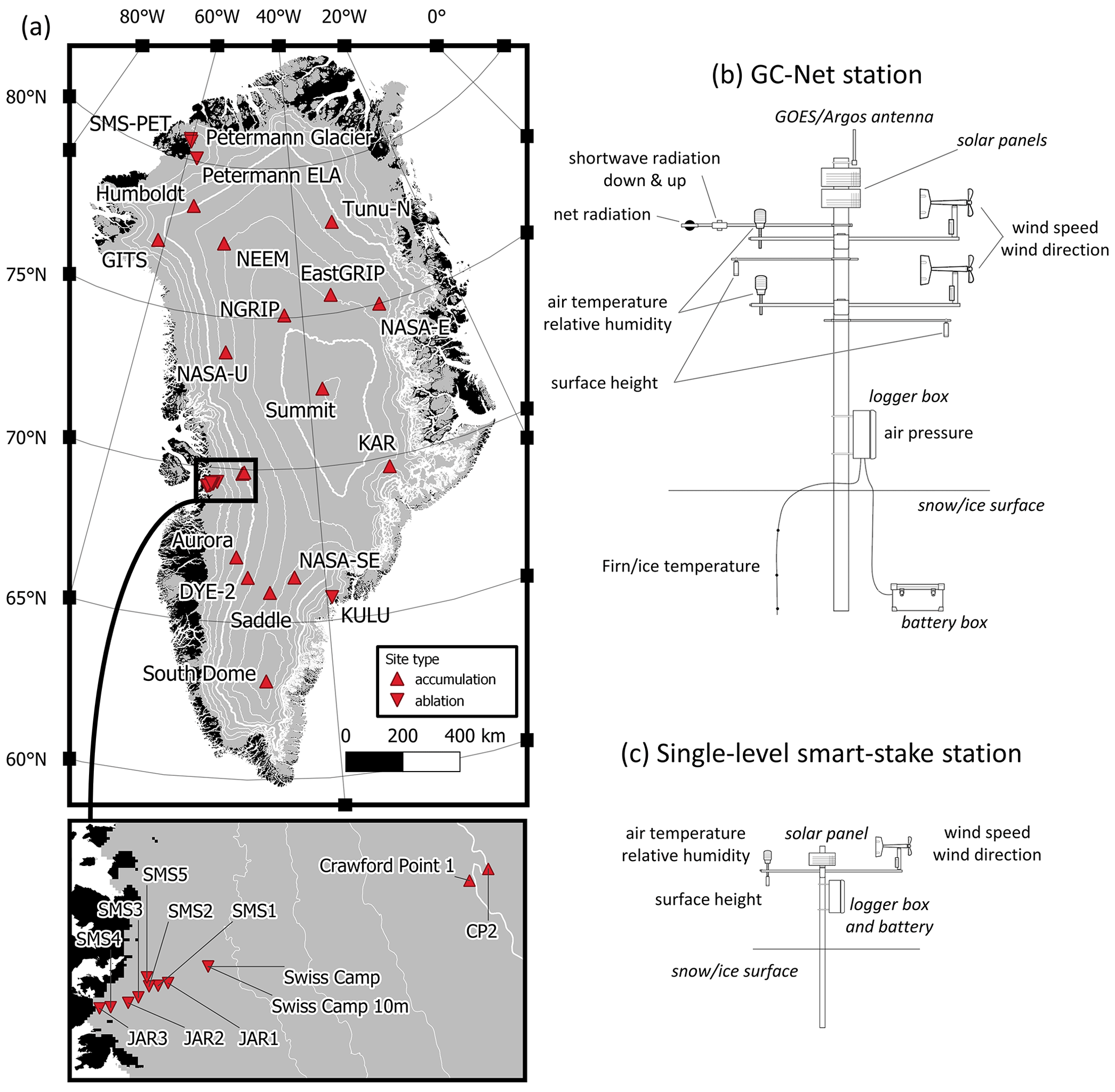
Figure 1(a) GC-Net weather stations in Greenland. Thick white lines are 2000 and 3000 m elevation contours, while thin white lines are 250 m elevation contours. (b) Design of the GC-Net weather station (two-level design). (c) Design of the single-level smart-stake station.
Table 1List of the GC-Net AWSs with coordinates (in the WGS84 reference system) and date of installation and decommission. The coordinates are the long-term average location or best available values. When possible, temporally resolved coordinates are also provided in the metadata.
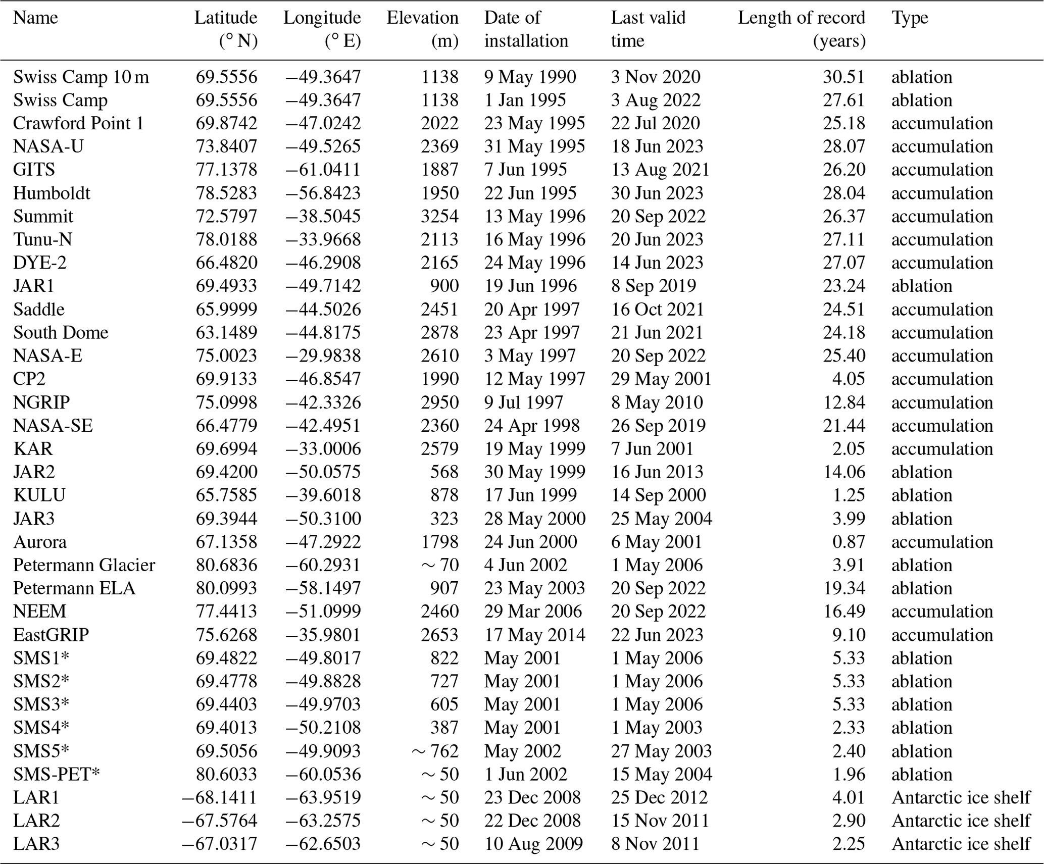
* Single-level smart-stake AWS
The GC-Net sites were partly chosen in synergy with existing science projects or existing logistic links. The GC-Net program was formally initiated in 1995, with the installation of the Swiss Camp, Crawford Point 1, NASA-U, GITS and Humboldt AWSs. The Swiss Camp 10 m meteorological tower had been operating since 1990 and continuously since June 1991 (Ohmura et al., 1991, 1992). The NASA-U, GITS and Humboldt stations were established in tandem with ca. 500 m deep ice-coring studies sponsored by NSF and NASA (Bales et al., 2001a, b; Mosley-Thompson et al., 2001, 2005). GITS (Greenland Ice Training Site) is located ca. 5.5 km southeast of the Camp Century military base and ice core location, which, at the time, served as a practice skiway for the US 109th Air National Guard ski-equipped LC-130H. The Crawford Point 1 station was installed upstream of Swiss Camp to represent the percolation area, to extend the altitudinal profile to 2000 m and to connect that with the Summit AWS record (McGrath et al., 2013). The precise location of Crawford Point (selected by John Crawford, Jet Propulsion Laboratory, California Institute of Technology) is the place where both ascending and descending NASA satellite orbits of interest intersected the 2000 m elevation contour. This contour was the focus of an early PARCA mass balance perimeter (Thomas et al., 2000).
In 1996, four AWSs were installed. The Tunu-N AWS was installed in tandem with PARCA-sponsored coring, where ice sheet snow accumulation exhibits a large-scale minimum (Sigl et al., 2015). The DYE-2 AWS was installed at the former military station of the same name. DYE-2 carries forward a legacy of glaciology and climatology measurements associated with the initial construction of the military station in 1959. DYE-2, later known as Camp Raven, now serves as the practice skiway for the US 109th Air National Guard and is home to many other measurements (e.g., Samimi et al., 2021; MacFerrin et al., 2022). The JAR1 AWS was installed in the ablation area down glacier from Swiss Camp. The Summit AWS was installed ca. 1.4 km west of the GISP2 ice core that had been completed in 1993.
In 1997, the South Dome, Saddle and NASA-E stations were installed alongside NASA-sponsored shallow ice-coring (Mosley-Thompson et al., 2001) and firn densification work (Hamilton and Whillans, 2000). The South Dome station is situated at the highest point on the ice sheet's South Dome, while Saddle station is situated at the lowest point on the main ice sheet's topographic divide between Summit and South Dome. The same year, the CP2 station was installed ∼8 km northeast of the Crawford Point AWS to capture surface topographic undulation-scale accumulation and climate variability. In 1997, the NGRIP AWS was installed at the site of a deep ice-core-drilling site (Dahl-Jensen et al., 2002). NGRIP AWS was discontinued in 2010 when the drilling was completed.
In 1998, NASA-SE was the last PARCA site where an AWS was installed in tandem with firn coring. In 1999, the Kangerdlugssuaq Accumulation Region (KAR) AWS was installed, and the KULU AWS was installed within reach from Kulusuk Airport in east Greenland. The same year, the JAR transect in the ablation area west of Swiss Camp received its second station, JAR2. The KULU and KAR stations were both discontinued in 2000 and 2001 due to, among other factors, strong winds, high accumulation and the remoteness of east Greenland, making station maintenance particularly challenging.
In 2000, the Aurora AWS was installed on the ice sheet ∼150 km east of Kangerlussuaq in western Greenland in connection to an on-ice automobile test track. The AWS was discontinued in 2001 when the car-testing project stopped. Also in 2000, the JAR transect received its third and lowest station, JAR3. In 2002, Petermann glacier AWS was installed on the floating tongue of Petermann glacier in northwest Greenland, and the Petermann ELA AWS was installed in the following year. These two AWSs provided the surface climate data needed for the study of the ice–ocean interaction at Petermann glacier (Rignot and Steffen, 2008). The Petermann station was discontinued due to the presence of crevasses. Crevasses and low snow accumulation are also now challenging aircraft access to Petermann ELA. In 2006, the NEEM AWS was installed in preparation of the North Greenland Eemian Ice Drilling project (NEEM team, 2013). The NEEM AWS remained at that location after the drilling project finished, and a new AWS was installed at EastGRIP in 2014 when a new deep-drilling project started.
In 2001, five single-level smart-stake AWSs (Fig. 1c) were installed in the lower ablation area of Sermeq Avannarleq glacier (Albert, 2007), neighbor of Sermeq Kujalleq (Jakobshavn isbræ). These smart stakes were serviced by snowmobile from Swiss Camp until 2003 (SMS4–5) and 2006 (SMS1–3). JAR3 was discontinued in 2004 due to the upstream expansion of crevasses, and JAR2 was discontinued in 2013 for similar reasons.
Three AWSs were installed on the Larsen C ice shelf, Antarctica, in 2008 (Kuipers Munneke et al., 2017; McGrath et al., 2021). Given the similarities in the station designs and data structures, we include these three Larsen C stations in this curated level-1 (L1) data product version of otherwise Greenland-focused GC-Net data.
Beginning in August 2020, GEUS began maintaining the GC-Net stations at Swiss Camp and JAR1. In 2021, GEUS installed its replacement AWSs at Crawford Point 1, NASA-SE, South Dome, GITS, Saddle, NASA-U, NEEM and DYE-2. Existing stations were removed from the first four sites, DYE-2 was raised and serviced, and the remaining historical stations were left as they were. In 2022, DYE-2, Saddle, Humboldt, NEEM, NASA-E and Tunu-N were visited, but no maintenance was carried out apart from downloading data from the logger and raising the lower boom arm at NASA-E. Also in 2022, GEUS installed new AWSs at Humboldt, NEEM, NASA-E and Tunu-N next to the original AWSs. In 2023, GEUS decommissioned DYE-2, NASA-U, EastGRIP, Humboldt and Tunu-N. In the coming years, GEUS plans to visit Petermann ELA, NEEM, NASA-E, Swiss Camp and Summit; retrieve their data; and decommission the historical AWSs.
3.1 Station design and maintenance
The main characteristic of the GC-Net AWS is its two levels of measurements for air temperature, relative humidity, wind speed and direction. In the L1 dataset, the variables labeled with 1 (e.g., TA1) were measured or derived from the lower level. The variables labeled with 2 (e.g., TA2) were measured or derived from the upper level. The two levels are typically placed with 1.2 m vertical separation, although other spacing was used on occasions when the station could not be raised and when the lower level was at risk of getting buried by accumulating snow.
The most common GC-Net masts were aluminum tubes with 4′′ (10.16 cm) outside diameters, initially 6.4 m in length. Ablation area sites (JAR2-3, PET ELA, PET Glacier and the SMS) used a 3′′ (7.62 cm) mast. Both the 4′′ and 3′′ outside diameter mast tubes had 0.25′′ (0.635 cm) wall thickness. The masts were inserted into a ca. 3.2 m deep hole in a borehole made in firn using a core drill or in ice using a steam or mechanical drill. The JAR1 station was the only ablation area station with the 4′′ (10.16 cm) outside diameter mast. The masts were raised (accumulation sites) or lowered (ablation sites) using a 6 m high tripod and winch system (Fig. 2), separating the upper section of the mast, inserting an extension in the case of accumulation area sites (or removing a section at ablation sites) and then lowering the upper section back down onto the base mast section. Over time, the base pipe reached a length of up to 30 m at NASA-SE. Low-accumulation sites (e.g., Tunu-N, Humboldt, NASA-E) could be visited every 1 or 2 years. High-accumulation sites, particularly NASA-SE and South Dome, needed annual visits to prevent burial by accumulating snow. Ablation area sites also needed frequent visits to prevent the mast from melting out and the AWS from collapsing. It was not uncommon to find ablation area AWS masts leaning. Because of the initial (1995–ca. 2000) use of guy wires, differential compaction or the failure of one wire led to station tilt. When the station tilt was too critical, the mast was re-drilled (e.g., at DYE-2 in 2019 and 2021).
For information on the design of the meteorological tower and the pre-1995 AWS at Swiss Camp, more details can be found in Ohmura et al. (1991, 1992), Steffen (1995) and Steffen et al. (1996).
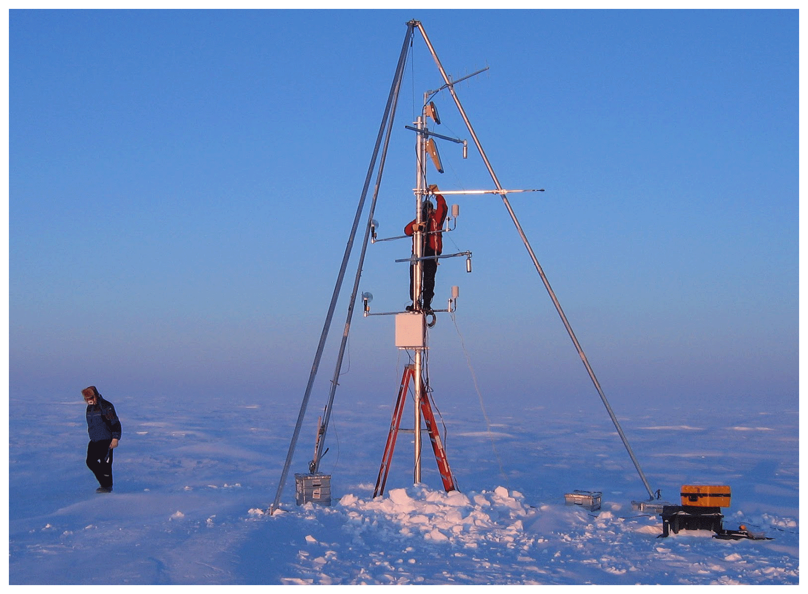
Figure 2Raising the Crawford Point 1 mast, 3 May 2005. Konrad Steffen (left), Russel Huff (right). Photo by Jason Box.
3.2 Instrumentation
The standard instrumentation of the GC-Net AWS is provided in Table 2, compiled from Steffen et al. (1996), Steffen and Box (2001), Box and Steffen (2001a), and Steffen et al. (2003, 2005, 2006). The primary air temperature measurement was done by a type-E thermocouple (variables TA1 and TA2 in the L1 dataset). Secondary air temperature readings were done by CS500 thermometers (variable TA3 for the lower level and TA4 for the upper level in the L1 dataset), but these sensors did not accurately measure temperatures below −40 ∘C. While efforts were made to keep the instrumentation consistent, exceptions include shifting the thermohygrometer from Vaisala INTERCAP 50YC (a.k.a. HUMICAP 180 packaged by Campbell Scientific as CS500) to the Vaisala HMP45 after ca. 1999 and, from ca. 2008, switching to the Vaisala HMP155. The Swiss Camp AWS had less consistent air temperature and hygrometer instrumentation as the site was used to test emerging technologies, including tests of fan-aspirated temperature shields. Barometers were initially a Vaisala PTB101A, replaced in ca. 1999 with a PTB101B. The LI-COR LI-190SZ instrument measuring downward and reflected shortwave radiation and surface albedo is sensitive to the 0.4–0.7 µm spectral range. The REBS Q7.1 net radiation sensor is sensitive to the 0.25–60 µm spectral range. A domeless version 1 Kipp & Zonen NR Lite net radiometer with a spectral range of 0.2–100 µm was used at Summit and Swiss Camp starting in ca. 2000. See Brotzge and Duchon (2000) for an intercomparison of the different radiometers. The snow, firn and ice temperatures were measured by 10 type-T thermocouples inserted in the snow, firn or ice with 1 m spacing, ranging from 1 to 10 m depth (Sampson, 2009). Most of these temperature strings were discontinued in 2010. The single-level smart-stake AWSs (Table 1) were not equipped with temperature strings. The surface height was measured with two SR50 sonic rangers. In the L1 dataset, these measurements are corrected for the effect of air temperature on the speed of sound according to the SR50 user manual (Campbell Scientific, 2007).
From 1995 to around 2000, the data logger was a Campbell Scientific CR10. These were replaced starting in 1999 with a CR10x until 2009 when CR1000 loggers were progressively introduced. The original Swiss Camp data loggers were CR21 and then CR21x, running the 10 m tower until ca. 1998.
Table 2Instrumentation overview.
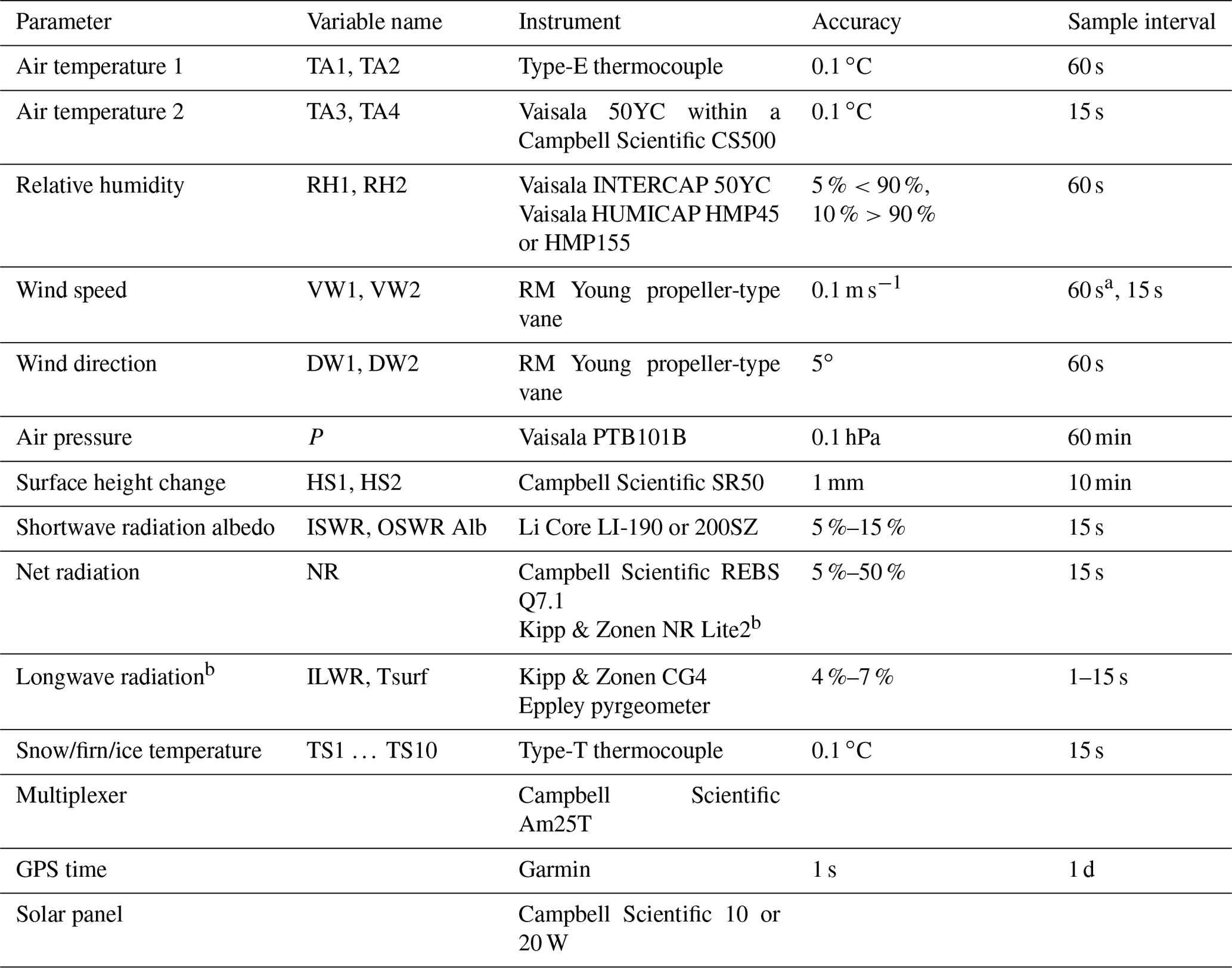
a Sampling was changed from 60 to 15 s after 1999 for all sites except NGRIP. b introduced at Swiss Camp and Summit in ca. 2000.
Two data collection systems were used to transmit the GC-Net AWS data in near-real time. For sites south of 72∘ N, the National Oceanic and Atmospheric Administration (NOAA) Geostationary Operational Environmental Satellites (GOES) system was used. For sites north of 72∘ N, the Argos polar-orbiting satellite system was used. Konrad Steffen found that the directional antenna for the more affordable GOES transmission worked at the higher-latitude NEEM and EastGRIP sites. These transmissions allowed near-real-time dissemination of the AWS data during the operation of the network. In the present dataset, data files retrieved from the loggers during site visits are used unless only transmitted data are available.
For the instrumentation of the meteorological tower and pre-1995 AWSs at Swiss Camp, more details can be found in Ohmura et al. (1991, 1992) and Steffen et al. (1995, 1996).
The GC-Net data have been processed with various software since GC-Net's creation. From 1995 to 2004, the GC-Net data concatenation of field-gathered or GOES/Argos transmissions was achieved using FORTRAN77 codes, followed by Interactive Data Language (IDL) scripts for the application of calibration constants and the filtering of outliers (Box and Steffen, 2001b). The GC-Net data processing was then migrated in 2004 to MATLAB scripts (Bayou and Steffen, 2011), where the user could exclude outliers via a graphical user interface. These two approaches lacked transparency and repeatability and were conducted using commercial software. For the GEUS-led reprocessing, processing scripts are written in Python using an open-source approach, allowing more transparency and straightforward repeatability via Git versioning (Vandecrux et al., 2023a). This re-processing could be done directly from the CR1000 logger files starting in 2009. For data collected by older loggers, the incomplete information about file headers and logger programs made it more complicated to work with these raw logger files. We therefore currently use historical files processed by Jason Box from 1995 to 2005 and by Nicolas Bayou and Konrad Steffen from 2005 to 2009 as input for our work. For the Swiss Camp 10 m meteorological tower, both logger files and historical FORTRAN processing scripts were available so we could re-process the raw logger files and apply the same calibrations as in the historical FORTRAN programs. The key steps of our transparent and open-source re-processing framework are detailed in the following paragraphs and in Fig. 3.
The re-processing of the historical GC-Net data presented here follows the FAIR principles (Wilkinson et al., 2016) where (i) both data and crucial metadata are findable through this publication and through the referencing of the Dataverse on common web search platforms; (ii) (meta)data are accessible through an open and free data distribution platform; (iii) the data are interoperable as the (meta)data are distributed in non-proprietary, machine-readable format; (iv) the (meta)data are reusable as the data are fully described and processed in a transparent way.
4.1 Data processing, filtering and adjustments
Ideally, the data processing should start from unaltered logger files (the level-0 dataset, L0); however, because the data loggers used before 2009 had changing file formats and no header, we use historical, processed and calibrated files (as produced for Box and Steffen, 2001a) until ca. 2009, when CR1000 data loggers were introduced. To build the level-0 merged dataset (L0M, Fig. 3), which is the starting point of our re-processing, we collect the available CR1000 logger files, apply the calibration coefficients to the radiation data and append them to the pre-CR1000 historical processed files. The data are then processed as illustrated in Fig. 3. The first step is to remove periods where the sensor and/or the station was not functioning and where no valuable information could be retrieved from the data. For each station, a CSV (comma-separated value) flag file lists these erroneous periods along with the sensor they apply to. The CSV flag file also contains for each flagged period a comment field explaining the reason for flagging, and the operator who applied the flag can be indicated. The processing script reads this station-specific flag file and discards the listed variables for the given periods.
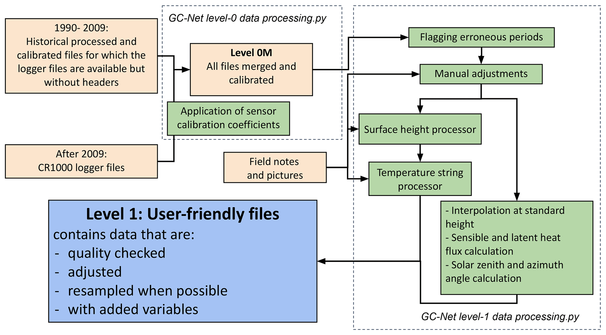
Figure 3GC-Net data-processing flow. Orange boxes indicate intermediate data products, green boxes indicate operations, and the blue box indicates the final L1 data.
The next step adjusts the data for biases and filters noisy measurements. Filtering is done with another series of station-specific adjustment CSV files. Each adjustment file contains a list of time periods, variables, adjustment function names and adjustment parameters for a given station. The target variables can be passed as a list of space-separated variables or as a regex (regular expression) string. The adjustment function names are self-explanatory (e.g., add, multiply, rotate, swap_with_, min_filter, max_filter). The processing script then applies the given function to the listed variables during the specified period. These adjustments allow us, for example, to correct for wind direction installed with an offset of 180∘, therefore giving rotated wind direction; to adjust for a shift in air pressure due to a missing or changing offset in the barometer measurement; or to construct the augmented or added variables listed in the next section (height of the wind sensors, continuous surface height). A comment for each modified period reports the motivation, e.g., a reported sensor malfunction, power failure, frozen anemometer propeller or unlikely values after comparison with an external dataset. When the suspicious data and their adjustments are discussed online on the project's issue page (https://github.com/GEUS-Glaciology-and-Climate/GC-Net-level-1-data-processing/issues, last access: 30 November 2023), the URL to the discussion is given in the comment field of the flagging or adjustment file. Attention was given to harmonize relative humidity into values relative to saturation water vapor pressure over water so that they can be converted into values relative to saturation water vapor pressure over ice later in the processing script (see next section). All these adjustments were determined through the evaluation of station photos (Box et al., 2023b), field notes (Vandecrux et al., 2023b), and comparisons with secondary AWS and regional climate outputs (Vandecrux, 2023). Time shifts were applied to many stations to compensate for data logger clock drift. These time shifts were persistent at Humboldt, where the logger clock was shifted by several months every year. The value of the time shift correction was chosen based on available field notes and on the comparison of the measured air pressure and temperature with values from the Regional Atmospheric Climate Model, RACMO (Noël et al., 2019).
Once the erroneous periods are removed and the adjustments applied, a last set of standard filters are applied: (1) a set of standard minimum and maximum filters is defined in a “filter” CSV file, first giving limits for each variable at all or some stations (time-specific min or max need to be listed in the adjustment CSV file); (2) a persistent value filter that detects periods where values do not change (e.g., anemometer covered in rime); and (3) the removal of non-meaningful data such as wind direction in the case of low (<0.5 m s−1) wind speed or isolated surface height measurements. The report of the data treatment is compiled in a single file, available here: https://github.com/GEUS-Glaciology-and-Climate/GC-Net-level-1-data-processing/blob/main/out/report_with_toc.md (last access: 30 November 2023).
The idea behind the open and transparent processing of the GC-Net data is that data users can investigate the site or variable of their interest and see what type of filtering or adjustments have been applied. Data users can post issues on the processing repository with questions or point at sensor malfunctions not yet removed from the data. Thereby, this transparent interaction with the data from all users can benefit all users. This flagging and adjustment framework, developed and tested on the GC-Net dataset, is now also used for operational PROMICE AWSs (https://github.com/GEUS-Glaciology-and-Climate/PROMICE-AWS-data-issues, last access: 30 November 2023).
4.2 Augmented, corrected and added variables
The GC-Net L1 dataset contains several variables that are derived or adjusted from the L0 data (e.g., instrument heights, relative humidity corrected for subfreezing conditions) and other variables that are added to the dataset to make the dataset easier to use (e.g., solar zenith and azimuth angles, time-stamped station position).
Instrument heights. Each station is equipped with two sonic rangers measuring the distance between each sensor and the surface (Table 2, Fig. 1b). However, these sensors are not installed with a fixed height offset compared to the height-sensitive measurements (air temperature, relative humidity, wind speed and direction). Additionally, the offset between the sonic ranger and the other instruments changes for each station and can also change through time as the station is maintained. Consequently, the sonic ranger heights from the L0 data are converted into instrument heights (HW1 and HW2) in the level 1 dataset by a series of time-specific adjustments to match the instrument height reported during station maintenance (Fig. 4). The maintenance data, digitized from field books (Vandecrux et al., 2023b), are compiled in a spreadsheet that is also available in the metadata folder of the L1 dataset. For periods and sites where no measurements of sensor heights were reported, a photogrammetric estimation of instrument heights (Box et al., 2023a) was derived from available photos (Box et al., 2023b). In the L1 data, we made HW1 or HW2 match with the reported or estimated heights of the anemometer. On a leveled GC-Net AWS, the anemometer height should be the same as the TA and RH sensors. However, on many occasions, the tilt of the station (not recorded) led to obvious differences between the reported height of the TA and RH sensors and the reported HW (Fig. 4). This error is currently not accounted for in the L1 product but can be investigated through evaluation of the field books, maintenance spreadsheet and the photo archive (Box et al., 2023b).
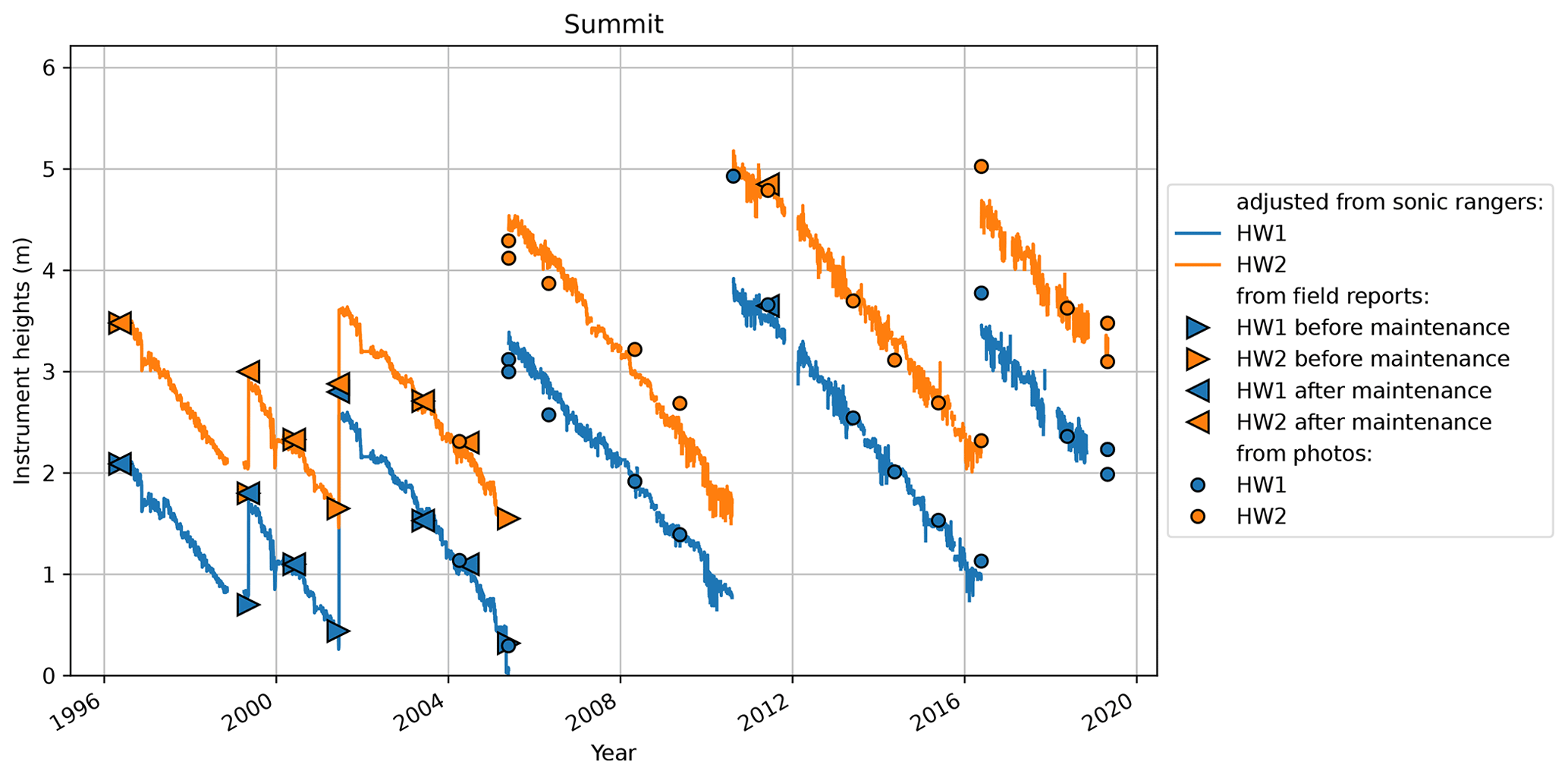
Figure 4Instrument heights for the Summit AWS. Triangles are instrument heights measured by operators in the field (pointing right: before maintenance, pointing left: after maintenance), while the dots are heights estimated from field pictures.
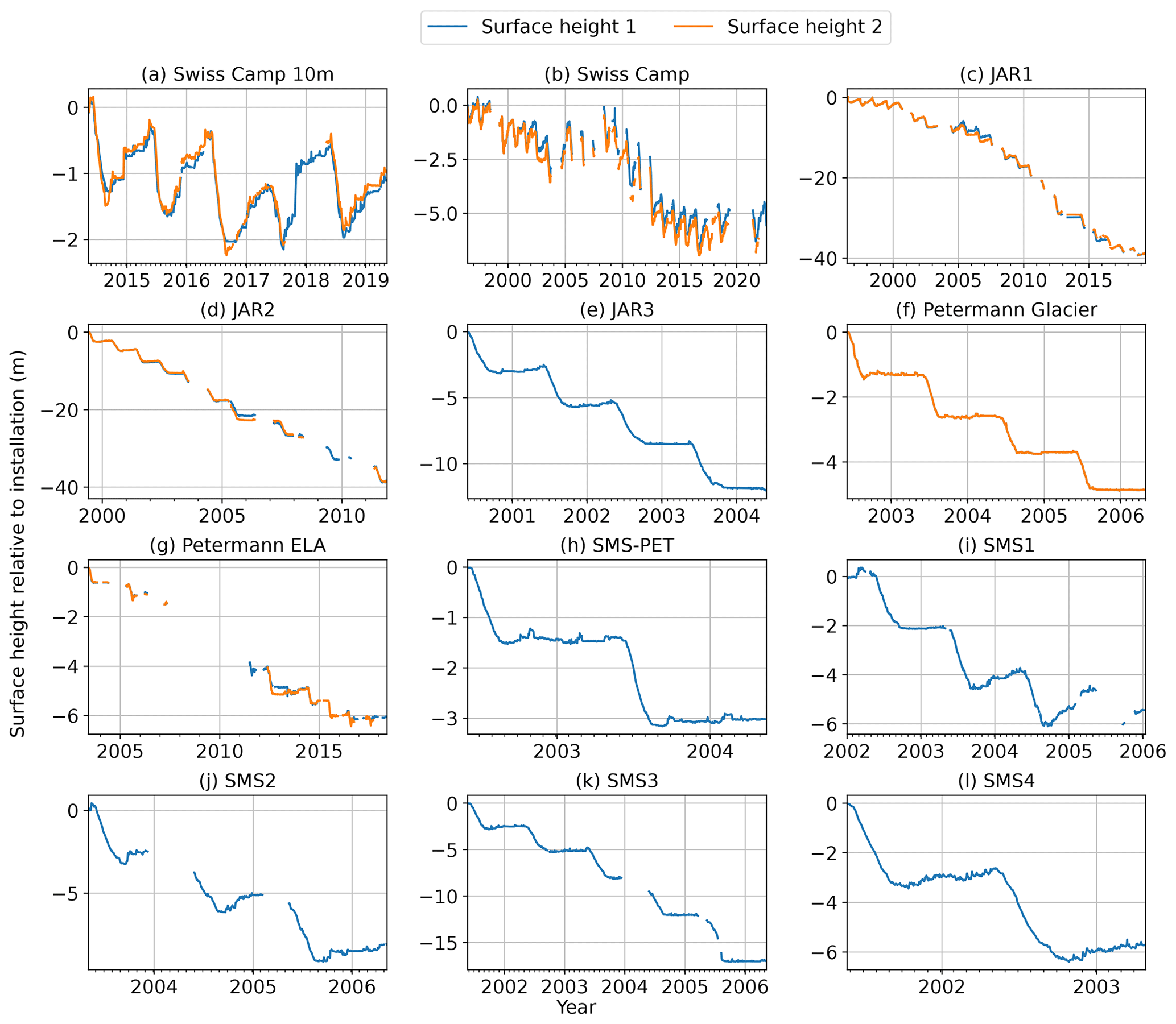
Continuous surface height. The raw sonic ranger heights (HW1 and HW2 in the L0 dataset) and the height of the instruments (HW1 and HW2 in the L1 dataset) include jumps whenever the station or an instrument was shifted up or down. We reconstruct a continuous surface height (HS1 and HS2 in the L1 dataset) by removing all these jumps in HW1 and HW2. The results at different stations appear in Figs. 4 and 5. The zero-height reference is arbitrarily set to the first recorded value. In cases when the sonic rangers were failing, the height after the gap was adjusted so that the trend was preserved, though the assumption of a purely linear trend means that data users should consider only the continuous periods for quantitative inferences.
Relative humidity correction and specific humidity calculation. The capacitance hygrometers used on the GC-Net stations respond to relative humidity with respect to water. Thus, under sub-freezing conditions, Goff–Gratch equations (Goff and Gratch, 1946) are used to calculate the corrected relative humidity (RH1_cor and RH2_cor in the L1 dataset) with respect to ice (Anderson, 1994, 1995). These corrected RH values are then converted into specific humidity (Q1 and Q2 in the L1 dataset). Relative correction and specific humidity calculations are done following the same scheme used for PROMICE AWS data (Fausto et al., 2021), now available through the pypromice Python package (How et al., 2022b).
Net radiation corrected from wind effect. The observations from both the REBS Q7.1 and Kipp & Zonen NR Lite instruments are affected by the wind-driven, convective cooling of the instrument and are consequently corrected as specified by the manufacturers (Campbell Scientific, 1996; Kipp & Zonen, 2023). The corrected values are available under the NR_cor variable in the L1 dataset.
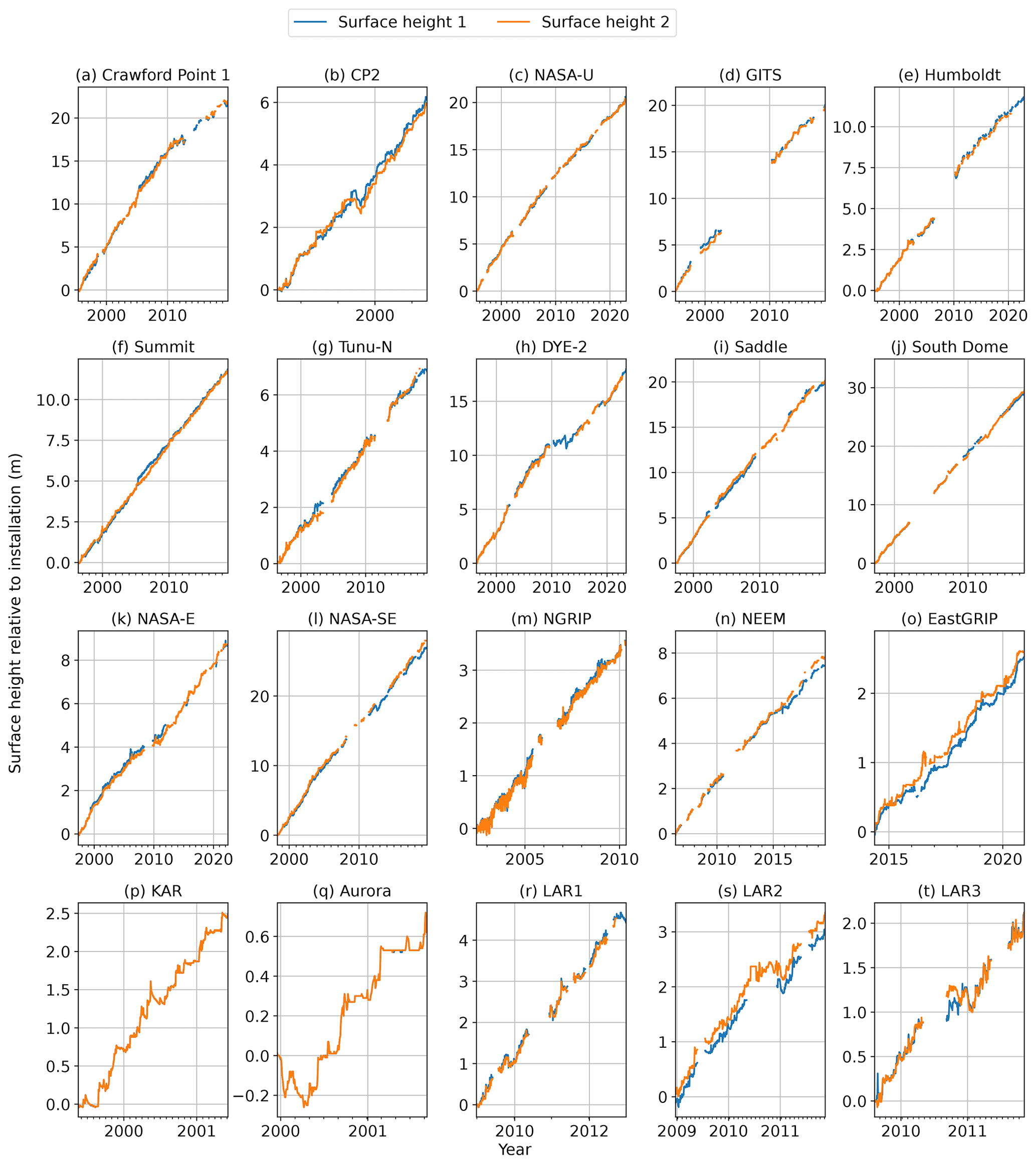
Figure 5Overview of the reconstructed surface height for the GC-Net sites located in accumulation regions.
Solar zenith and azimuth angles. The solar azimuth (SAA) and zenith angles (SZA) are key variables when using any in situ irradiance measurement. We calculate, for each station location, SZA and SAA using the pypromice Python package (How et al., 2022b).
Surface albedo. The surface albedo is calculated from hourly averages as the ratio of the reflected to downward shortwave irradiance. Hours with SZA >70∘, low illumination conditions (ISWR or OSWR <100 m W−2) and impossible albedo values (≤0 or ≥1) are discarded. The calculated albedo is very sensitive to instrument level and periods with frost obscuring one or both of the pyranometers. We therefore advise the use of the more robust daily average albedo values or a running hourly integration of daily values, such as that presented in van den Broeke et al. (2004) and Stroeve et al. (2013). We recommend caution when using the hourly albedo values until further assessments and corrections of pyranometer sensor tilt are made. See Sect. 5.4 for more detailed information.
Air temperature, relative humidity and wind speed at standardized height. In addition to the measurements at the two levels, the air temperature, relative humidity and wind speed are also provided at 2, 2 and 10 m (variables TA2m, RH2m, VW10m). For TA2m and RH2m, the interpolation and extrapolation are done linearly from the two measurement levels. For VW10m, we first extrapolate to 10 m using a logarithmic fit on the two measurement levels. If only one level is available or if the wind speed at the lower level is higher than at the upper level, the logarithmic fit cannot be used, and we then estimate the 10 m wind speed using the uppermost available measurement and a theoretical logarithmic wind profile with a surface roughness length of 0.01 m (as used by Konrad Steffen in a previous release of the GC-Net data).
Turbulent heat fluxes. The purpose of the two levels on the GC-Net AWS is to capture the near-surface gradients in TA, RH and VW and to derive the turbulent sensible and latent heat fluxes resulting from these gradients (e.g., Box and Steffen, 2001a; Cullen et al., 2014). The sensible and latent heat fluxes (SHF and LHF) are calculated using the method from Steffen and DeMaria (1996) as coded in the JAWS Python package (Zender et al., 2018). SHF and LHF calculations are sensitive to the data quality and accuracy of the instrument heights (Box and Steffen, 2001a) and should be used with caution.
Depth of the temperature strings and 10 m ice and/or firn temperature. The GC-Net AWSs monitor snow, ice and firn temperatures through 10 thermocouples (Fig. 1b). The depth of each sensor (DTS1-10 in the L1 dataset) is estimated for each time step from the available installation depth reported in field books and from the continuous surface height following a similar procedure as in Vandecrux et al. (2020). Compaction of the firn between the sensors is not accounted for in the L1 dataset, although Vandecrux et al. (2020) found that, in the first year following the installation, firn compaction reduces the spacing by ca. 15 % near the surface and by ca. 3 % down to 10 m depth. The ice or firn temperature at a standardized 10 m depth (TS_10m in the L1 dataset) below the surface is linearly interpolated or extrapolated from the available measurements with the condition that at least one sensor is located within ±1.5 m from the 10 m depth.
Station position through time. Over the 3 decades of measurements, the ice on which the GC-Net AWSs are standing has been advected towards the ice sheet margin due to ice flow. We compiled all the available GPS measurements to document the AWS displacements (Vandecrux and Box, 2023). For the stations located in areas of faster ice flow (Swiss Camp, Crawford Point 1, NASA-U, GITS, Tunu-N, DYE-2, JAR1, NASA-E, NASA-SE and Petermann-ELA) and when sufficient GPS measurements are available, we interpolate or extrapolate the hourly positions of the stations by fitting a first-order spline to the observed coordinates. These interpolated or extrapolated coordinates are available in L1 data files as Lat and Lon. The interpolation is done using a spline best fit and therefore does not exactly match observations when available but rather looks at the trend in sets of observed coordinates. This approach was more robust in relation to inaccuracies in some of the handheld GPS positions. For the remaining stations (not moving or insufficient GPS measurements), the coordinates from Table 1 are included in the Lat and Lon variables in the L1 data files. An example of these measured and interpolated or extrapolated annual coordinates is given in Fig. 7 for JAR1 AWS.
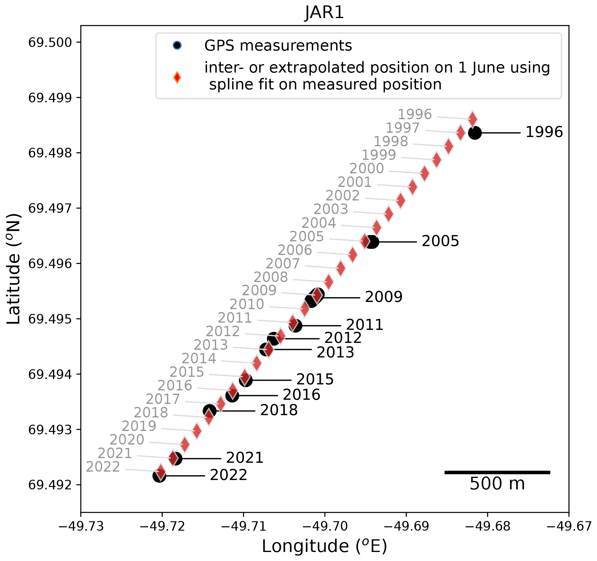
Figure 7Example of handheld GPS observations of JAR1 AWS position (black dots) and interpolation to annual position using a spline fit of the observations (red diamonds).
5.1 Format and structure
The GC-Net level-1 dataset is made available in Non-binary Environmental Archive Data (NEAD) format, which is a CSV file with an added metadata header. The format is described in Iosifescu Enescu et al. (2020), and the pyNEAD Python package (Mankoff and Vandecrux, 2023) is used to read and write NEAD files. The GC-Net level-1 dataset contains both hourly and daily values in their respective folders, and, respecting the historical distribution of GC-Net data, the time stamp was set to the end of the measurement interval and documented accordingly in the NEAD file header. The data are divided into a folder for hourly averages and a folder for daily averages. A README text file and CSV files listing the AWS reference coordinates and the variables contained in the L1 dataset are available in the dataset root directory. The compilations of maintenance reports from the AWS are available in Vandecrux et al. (2023b), the field picture archive is stored in Box et al. (2023b), and the collection of observed GPS coordinates is available in Vandecrux and Box (2023).
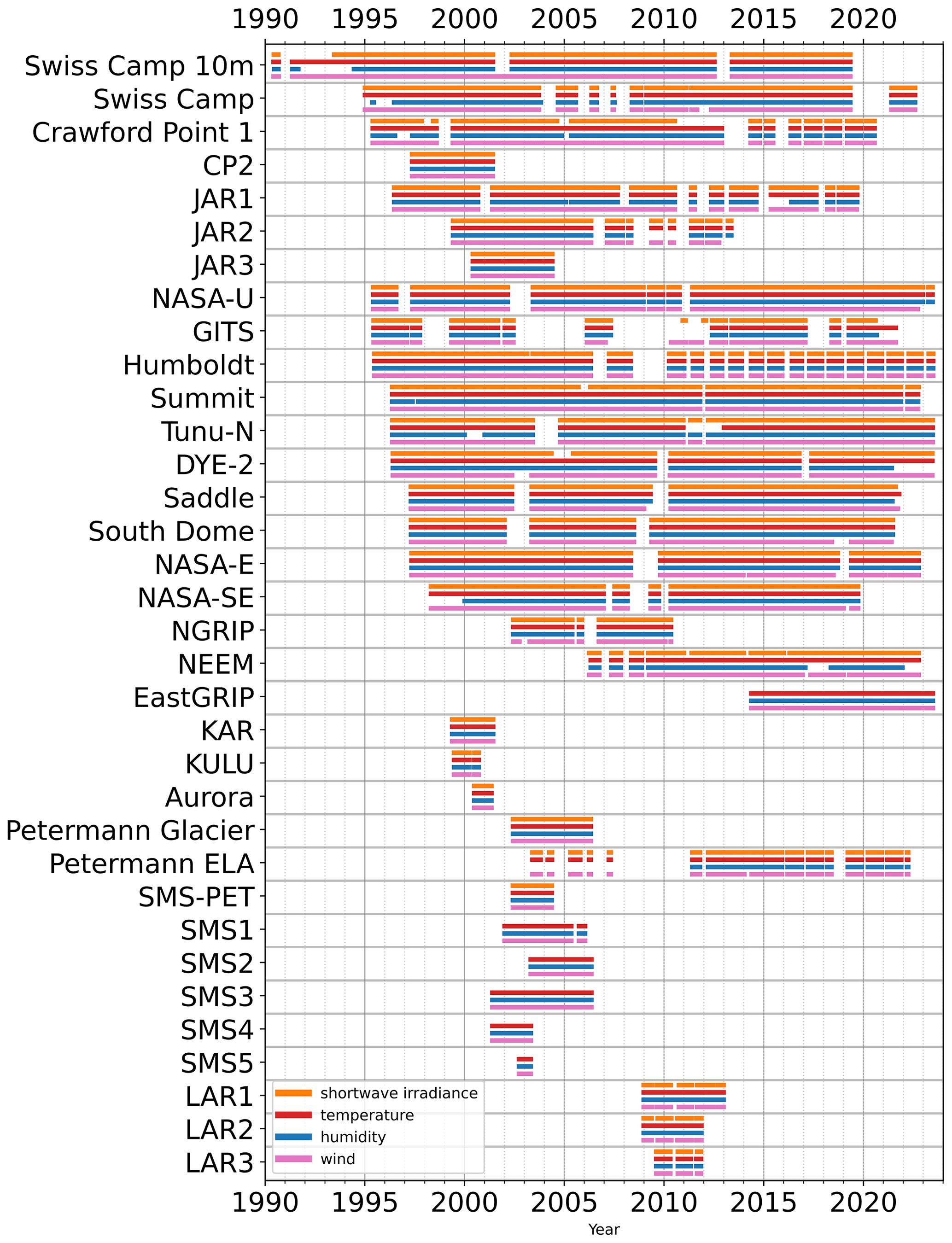
Figure 8Data availability for shortwave irradiance, air temperature, humidity, and wind speed and/or direction.
5.2 Data coverage
Operating a weather station on the Greenland Ice Sheet is a technical and logistical challenge. The instrumentation, power management and data storage strategies were designed to withstand these harsh conditions. Yet, many issues were reported through the years, and these failures include, among others, power shortages or short circuits (e.g., repeatedly at the GITS AWS); cables being pulled due to snow compaction; AWSs getting buried when site visits were not made; AWSs in the ablation area melting out and collapsing (mainly JAR1-3 and SWC AWSs); logger clock malfunctions (e.g., repeatedly at Humboldt); or individual sensor failures due to extremely low temperatures, rime or liquid water. An overview of the data availability for the four main variables (shortwave irradiance, air temperature, humidity, and wind speed and/or direction) is provided in Fig. 8.
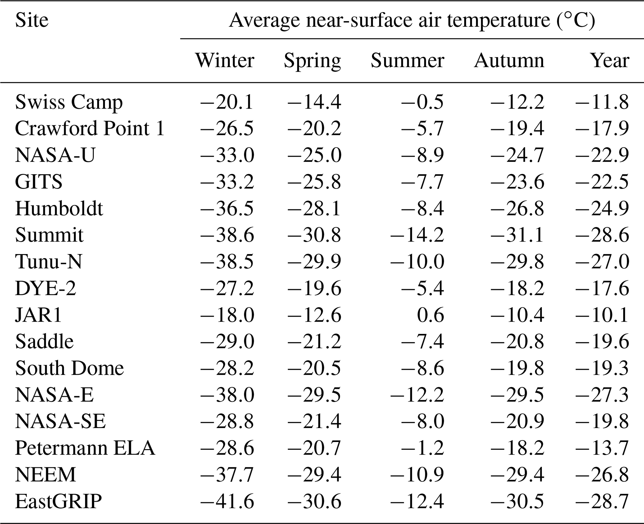
Table 3Seasonal average near-surface air temperature. The interpolated 2 m air temperature is used when the two levels are available; otherwise, a single measurement level is used.
5.3 Climatology at the GC-Net sites
The GC-Net weather stations are located primarily in the higher-elevation accumulation zone of the ice sheet, with near-surface air temperature remaining below freezing year round (Fig. 9) and annually increasing surface heights due to snow accumulation (compensated for by the ice sheet motion, which is not measured by the AWS). The lowest average temperatures are found at Summit station (Table 3), at the topographic high point of the ice sheet (3254 m a.s.l.). The Swiss Camp, JAR and Petermann stations, which represent relatively higher temperatures at or below the ELA, are characterized by above-freezing summer air temperatures (Table 3) and net annual ablation (loss in surface height).
All sites exhibit a distinct summer season between day of the year 100–300, characterized by a peak in near-surface air temperature during the warmest month of July (Fig. 9). When compared to the winter season, the summer season shows lower variability in near-surface air temperature and relatively low wind speeds (Figs. 9 and 10). The winter season is characterized by a prolonged period of consistently lower temperatures and higher winds, spanning December through February (Figs. 9 and 10).
Many GC-Net stations are approaching a climatologically significant time span (∼30 years), providing valuable records of long-term trends in both air temperature and surface height change.
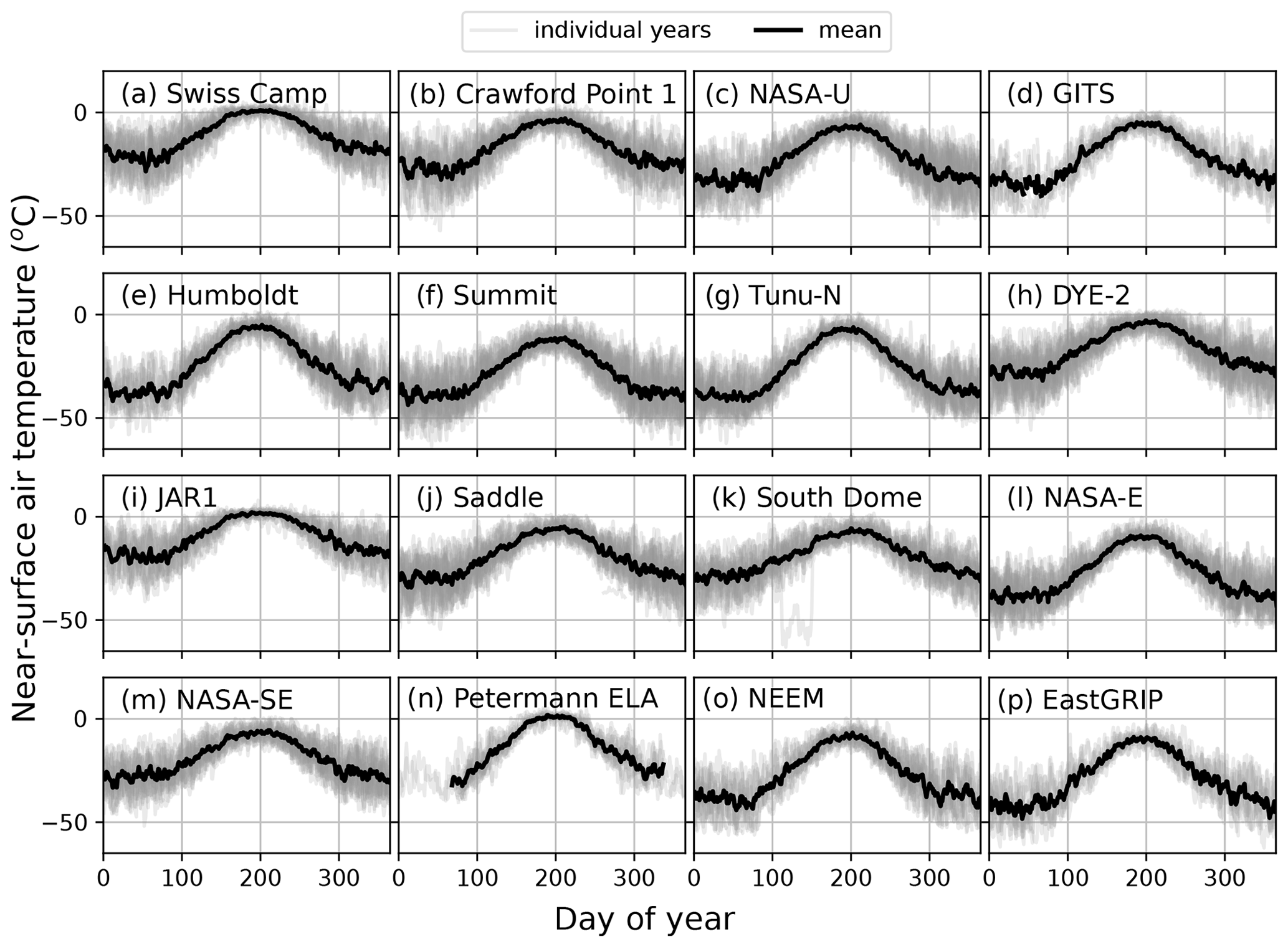
Figure 9Climatology of daily near-surface air temperatures. The interpolated 2 m air temperature is used when the two levels are available; otherwise, a single measurement level is used. Climatological values are calculated when values for at least 5 years are available.
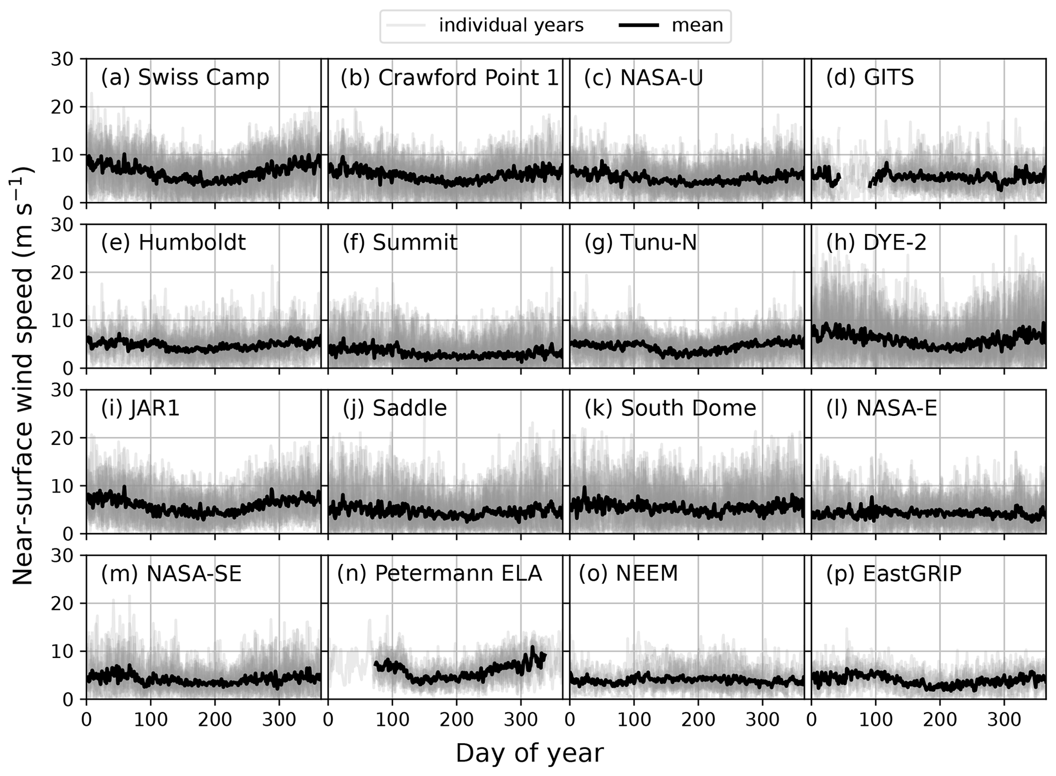
Figure 10Climatology of the near-surface wind speed. An extrapolated 10 m wind speed is used when the two levels are available; otherwise, the available level is used. Climatological values are calculated when values for at least 5 years are available.
5.4 Dataset evaluation and known limitations
With the longevity of some stations (e.g., more than 30 years at Swiss Camp), questions can be raised about the quality and accuracy of the sensors that have been deployed for several years, i.e., sensor drift and deterioration. Here, we evaluate the air temperature, relative humidity, wind speed, and downward and upward shortwave irradiance at nine GC-Net sites relative to independent AWS data during the 2007–2022 period. At Swiss Camp, NASA-E, NASA-U, NEEM, Saddle and DYE-2, the GC-Net data are compared, respectively, to measurements from the SWC, NAE, NAU and NEM AWSs installed by GEUS within 500 m of the GC-Net stations (GEUS, 2020; How et al., 2022a). DYE-2 data are also compared to measurements from Samimi et al. (2021). The GC-Net station at Summit is compared to the nearby (within 2 km) DMI and NOAA measurements. The metrics presented in Table 4 can be considered to be the overall assessment of the relative accuracy and a conservative measurement for the repeatability of the GC-Net data.
Table 4Comparison of the GC-Net AWS data to independent AWS observations at the GC-Net sites. MD stands for mean difference, and RMSD stands for root mean squared difference.
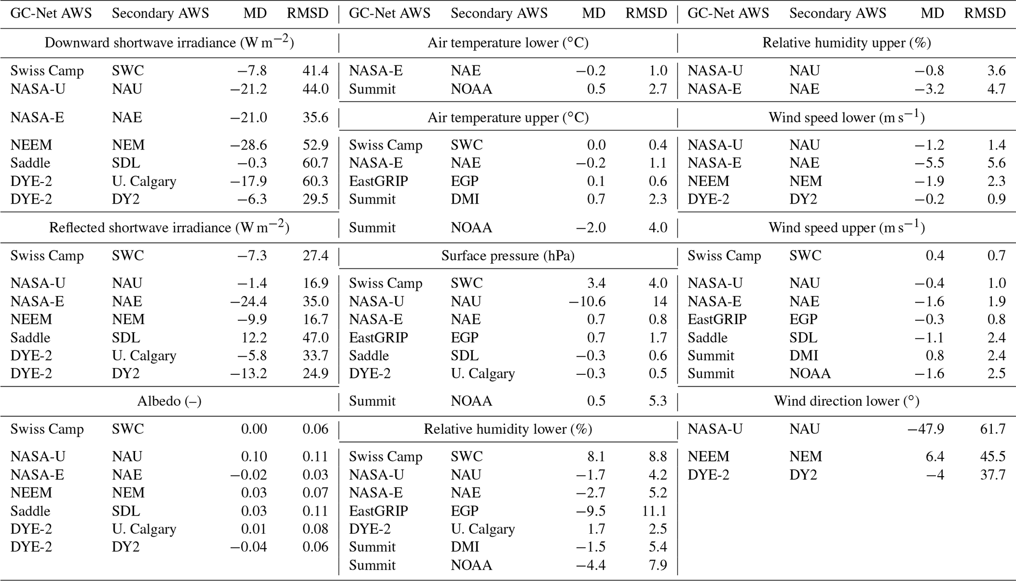
Some of the discrepancies between the different AWS measurements in Table 4 are likely due to known limitations of the GC-Net AWS instruments. The GC-Net air temperature measurements were naturally aspirated, i.e., not ventilated using motorized fans, and are therefore subject to solar overheating under low wind speed and high shortwave irradiance (Steffen and Box, 2001; Box and Steffen, 2001a). Studies in Antarctica have reported temperature differences of up to 8 ∘C between ventilated and non-ventilated measurements (Genthon et al., 2011; Morino et al., 2021). However, by comparing the GC-Net measurements to the air temperatures values from actively ventilated instruments on the newer AWSs installed at the GC-Net sites (Table 4), we found that this effect can be very site specific. When comparing 12 collocated pairs of ventilated and unventilated instruments in low-wind-speed conditions (<2 m s−1) and with high downward shortwave irradiance (>200 W m−2), the linear correlation between unventilated-to-ventilated temperature differences and downward shortwave irradiance was significant (P<0.05) in a minority of four cases, while the remaining eight comparisons showed no significant correlation between temperature difference and downward irradiance.
The hygrometers are sensitive to the harsh conditions on the ice sheet and are prone to degradation. Ohmura et al. (1991, 1992) also noted issues with the absolute calibration of the hygrometers installed at Swiss Camp in 1990–1993. The main limitations of hygrometers are their inability to measure supersaturation, the clogging of the porous sensor when the ambient air is saturated or supersaturated, and slow de-clogging when conditions are dry again (Anderson, 1995). Data quality can be judged visually from RH time series, especially in dry and windy regions: the reading will remain constant at 100 % with regards to ice and then suddenly dip to more realistic drier values.
The downward and reflected shortwave irradiance measurements, as well as the albedo derived from them, are known to be sensitive to the leveling of the instrument (Wang et al., 2016) and the surface slope (Weiser et al., 2016; Picard et al., 2020). Apart from photogrammetric assessments, which are challenging and from very limited field notes, the tilt of the GC-Net AWSs was not measured over the years. Wang et al. (2016) presented the retrospective, iterative, geometry-based (RIGB) tilt correction method that estimates the tilt of the station from its measurement of downward shortwave irradiance during clear-sky days. Unfortunately, the resource files required by this algorithm (the theoretical downward shortwave irradiance against which the measurements are to be compared) were discontinued after 2015. We have begun working on applying the method to the GC-Net data as part of a future release. Until this correction has been applied, we advise caution when using the radiation and albedo data.
The shortwave irradiance and wind speed measurements are subject to the shadowing of the station: the former when the station's shadow passes over the sensor and the latter when the anemometer is downwind of the station. These issues were minimized through the design of the station by installing the pyranometer boom, directed south, or the anemometers across from the predominant wind direction. Additionally, under certain conditions (e.g., when the station stands high above the surface), the station mast and logger box may enter the field of view of the pyranometer. Consequently, the AWS may mask part of the diffuse irradiance from the snow. This effect can be corrected, for example, for the albedo values in Eq. (16) of Aoki et al. (2011), but the exact geometry and tilt of the station are required. This is not considered here but may be pursued in future data releases.
The type-T thermocouples measuring snow and ice temperature are subject to noise (Cathles et al., 2007; Sampson, 2009). The cause is that thermocouples only measure the temperature difference between a given depth and a reference junction in the logger box, and this reference temperature appeared to be insufficiently stable, thereby affecting all measurements synchronously. This synchronous noise does not affect all sites equally, and caution is recommended depending on the site and use of these snow and ice temperature data.
Through this review of potential measurement errors, we do our best to highlight potential issues for the data users, especially for applications highly sensitive to data quality. Nevertheless, these errors should be sporadic, and the majority of the record can be considered to be a robust measurement of the surface climate within the uncertainty linked to the sensors (Table 2) and the practical uncertainty found through comparison with other AWSs (Table 4).
The stable version of the GC-Net level-1 dataset is available at https://doi.org/10.22008/FK2/VVXGUT (Steffen et al., 2023). The pyNEAD Python package is recommended for reading these files. Although many of the AWSs have been discontinued, the level-1 dataset is to be refined through an iterative process of identification and removal of spurious data and potential adjustments of measurements. Data users are encouraged to ask their questions and report issues at https://github.com/GEUS-Glaciology-and-Climate/GC-Net-level-1-data-processing/issues (last access: 30 November 2023, Vandecrux et al., 2023a). The maintenance reports from the AWS are available at https://doi.org/10.5281/zenodo.7728549 (Vandecrux and Box, 2023b), and the fieldwork pictures sorted by site and year are available at https://doi.org/10.5281/zenodo.7839788 (Box et al., 2023b).
For each new release of the level-1 dataset, the processing scripts will be captured in a code release on the GC-Net level-1 data-processing repository (https://github.com/GEUS-Glaciology-and-Climate/GC-Net-level-1-data-processing, Vandecrux et al., 2023a). This repository also contains diagnostic plots and codes used to produce Figs. 4 and 5. The GPS coordinates' interpolation and extrapolation scripts, as well as the plotting code for Fig. 7, are available at https://doi.org/10.5281/zenodo.7729070 (Vandecrux and Box, 2023). The scripts used for the evaluation of the GC-Net data against independent AWSs and the study of the AWS climatology (Figs. 7–8 and Tables 3–4) are available at https://doi.org/10.5281/zenodo.7728938 (Vandecrux, 2023). The pyNEAD Python package is archived at https://doi.org/10.5281/zenodo.7728587 (Mankoff and Vandecrux, 2023).
The level-1 reprocessing of the historical GC-Net AWS data brings the GC-Net data to a higher-quality standard, distributed under the FAIR principles (Wilkinson et al., 2016). This ultimately paves the way to merging these records with data from the modern GC-Net AWS that have been installed by GEUS at the GC-Net sites since 2021. In addition to the iterative procedure of the identification and removal of residual erroneous data through an inclusive community effort via the GitHub issues page, future work should focus on establishing solar irradiance tilt correction and the study of the long-term effect of firn densification on surface height records.
The GC-Net AWSs represent the most widespread and longest consistent meteorological dataset on the Greenland Ice Sheet, with the monitoring sites having reached, or approaching, a climatologically significant time span. The GC-Net data can be used for long-term climate evaluation but also for process-oriented studies and as ground truth for remote sensing products and regional climate models. These datasets are therefore an essential and valuable asset to assess the response of the Greenland Ice Sheet to a changing climate.
KS led the GC-Net project, secured funding, maintained the stations and processed the data until 2020. BV coordinated the effort for the reprocessing, compiled the data and metadata, and drafted the paper. Substantial editing of the text was done by JEB, KDM, WTC, AR and PH. APA, RSF and SBA secured the funding for the visit to the GC-Net sites from 2020. DAH, PH, PJW, KDM and MKR contributed to the reprocessing scripts and visualization. IIE, RKB and DHA handled the transmitted data at WSL until 2022. DAH, SiS, DM, NB, NJC, MS, SaS, AH, BP, JW, HJZ, KSa, NPM and JEB accompanied and assisted KSt in the field until 2020. NBK, AR, KDM, WTC, APA, PH, BV and JEB visited and maintained the GC-Net sites after 2020. All the co-authors reviewed and approved the paper.
At least one of the (co-)authors is a member of the editorial board of Earth System Science Data. The peer-review process was guided by an independent editor, and the authors also have no other competing interests to declare.
Publisher's note: Copernicus Publications remains neutral with regard to jurisdictional claims made in the text, published maps, institutional affiliations, or any other geographical representation in this paper. While Copernicus Publications makes every effort to include appropriate place names, the final responsibility lies with the authors.
We acknowledge the key contributions from all the people that have participated in the GC-Net project, assisted Konrad Steffen through the years and contributed to the longevity of GC-Net. In particular, we acknowledge (in alphabetical order) the support from Robin Abbott, Waleed Abdalati, Todd Albert, Kate Daniels, Lucia Espona Pernas, Nena Griessinger, Alain Hubert, Russell Huff, Nighat Johnson-Amin, Mike MacFerrin, Molly McCallister, Reza Naderpour, Atsumu Ohmura, Allan Ø. Pedersen, Thomas, Philipps, Gian-Kasper Plattner, Kim Petersen, Martin Proksch, Christian Schneeberger, Christopher Shields, Martina Særrelse, Julienne Stroeve, Benjamin Walter, Øyvind A. Winton and many others. We thank three anonymous reviewers for their constructive comments.
From 1995 to 2020, the funding of GC-Net was secured by Konrad Steffen through several NASA and NSF grants (grant nos. NAPW-2158, NAG51-5651612, NAG5-10600, NAG5-10857, NNG06GB08G, and OPP-9423530). The transition of GC-Net to GEUS and the data reprocessing were funded by DANCEA (Danish Cooperation for Environment in the Arctic) under the Danish Ministry of Climate, Energy and Utilities. The Danish Finance Law currently supports GEUS for the continuation of GC-Net field and data activities.
This paper was edited by Di Tian and reviewed by three anonymous referees.
Ahlstrøm, A. P. and PROMICE project team: A new programme for monitoring the mass loss of the Greenland ice sheet, GEUS Bulletin, 15, 61–64, https://doi.org/10.34194/geusb.v15.5045, 2008.
Albert, T. H.: Assessment of glacier mass balances from small tropical glaciers to the large ice sheet of Greenland, PhD Thesis, Florida State University, https://doi.org/10.22008/FK2/DQRE71, 2007.
Anderson, P. S.: A Method for Rescaling Humidity Sensors at Temperatures Well below Freezing, J. Atmos. Ocean. Tech., 11, 1388–1391, https://doi.org/10.1175/1520-0426(1994)011<1388:AMFRHS>2.0.CO;2, 1994.
Anderson, P. S.: Mechanism for the Behavior of Hydroactive Materials Used in Humidity Sensors, J. Atmos. Ocean. Tech., 12, 662–667, https://doi.org/10.1175/1520-0426(1995)012<0662:MFTBOH>2.0.CO;2, 1995.
Andersen, M. L., Larsen, T. B., Nettles, M., Elosegui, P., Van As, D., Hamilton, G. S., Stearns, L. A., Davis, J. L., Ahlstrøm, A. P., de Juan, J., and Ekström, G.: Spatial and temporal melt variability at Helheim Glacier, East Greenland, and its effect on ice dynamics, J. Geophys. Res.-Earth Surf., 115, F04041, https://doi.org/10.1029/2010JF001760, 2010.
Aoki, T., Kuchiki, K., Niwano, M., Kodama, Y., Hosaka, M., and Tanaka, T.: Physically based snow albedo model for calculating broadband albedos and the solar heating profile in snowpack for general circulation models, J. Geophys. Res.-Atmos., 116, D11114, https://doi.org/10.1029/2010JD015507, 2011.
Aoki, T., Matoba, S., Uetake, J., Takeuchi, N., and Motoyama, H.: Field activities of the “Snow Impurity and Glacial Microbe effects on abrupt warming in the Arctic” (SIGMA) Project in Greenland in 2011–2013, B. Glaciol. Res., 32, 3–20, https://doi.org/10.5331/bgr.32.3, 2014.
Bales, R. C., McConnell, J. R., Mosley-Thompson, E., and Csatho, B.: Accumulation over the Greenland ice sheet from historical and recent records, J. Geophys. Res., 106, 33813–33825, https://doi.org/10.1029/2001JD900153, 2001a.
Bales, R. C., Mosley-Thompson, E., and McConnell, J. R.: Variability of accumulation in northwest Greenland over the past 250 years, Geophys. Res. Lett., 28, 2679–2682, https://doi.org/10.1029/2000GL011634, 2001b.
Bayou, N. and Steffen, K.: QCheck: a Matlab package for the processing of GC-Net automated weather station data, GitHub [code], https://github.com/GEUS-Glaciology-and-Climate/GC-Net-Matlab-processing-scripts, last access: 1 March 2023, 2011.
Braithwaite, R., Konzelmann, T., Marty, C., and Olesen, O.: Errors in daily ablation measurements in northern Greenland, 1993–94, and their implications for glacier climate studies, J. Glaciol., 44, 583–588, https://doi.org/10.3189/S0022143000002094, 1998.
Box, J. E. and Steffen, K.: Sublimation on the Greenland ice sheet from automated weather station observations, J. Geophys. Res.-Atmos., 106, 33965–33981, https://doi.org/10.1029/2001JD900219, 2001a.
Box, J. E. and Steffen, K.: FORTRAN and IDL processing scripts for the historical GC-Net data, GitHub [code], https://github.com/GEUS-Glaciology-and-Climate/JEB_GC-Net, last access: 1 March 2023, 2001b.
Box, J. E., Stroeve, J. C., and Abdalati, W.: Steffen, K., Abdalati, W., and Stroeve, J.: Climate sensitivity studies of the Greenland ice sheet using satellite AVHRR, SMMR SSM/I and in situ data, Meteorol. Atmos. Phys., 51, 239–258, https://doi.org/10.1007/bf01030497, 1993., Prog. Phys. Geogr.-Earth Environ., 45, 632–638, https://doi.org/10.1177/03091333211011368, 2021.
Box, J. E., Revheim, M., and Vandecrux, B.: GCNet_photogrammetry: GC-Net weather station geometry from field picture photogrammetry (Version v1), Zenodo [code], https://doi.org/10.5281/zenodo.7729252, 2023a.
Box, J. E., Vandecrux, B., Houtz, D., and Steffen, K.: GC-Net historical photo archive, Zenodo [data set], https://doi.org/10.5281/zenodo.7839788, 2023b.
Bromwich, D. H., Robasky, F. M., Keen, R. A., and Bolzan, J. F.: Modeled Variations of Precipitation over the Greenland Ice Sheet, J. Climate, 6, 1253–1268, https://doi.org/10.1175/1520-0442(1993)006<1253:MVOPOT>2.0.CO;2, 1993.
Brotzge, J. A. and Duchon, C. E.: A Field Comparison among a Domeless Net Radiometer, Two Four-Component Net Radiometers, and a Domed Net Radiometer, J. Atmos. Ocean. Tech., 17, 1569–1582, https://doi.org/10.1175/1520-0426(2000)017<1569:AFCAAD>2.0.CO;2. 2000.
Campbell Scientific: Q-7.1 Net Radiometer, Instruction Manual, https://s.campbellsci.com/documents/us/manuals/q-7-1.pdf (last access: 28 February 2023), 1996.
Campbell Scientific: SR50 Sonic Ranging Sensor, Instruction Manual, https://s.campbellsci.com/documents/au/manuals/sr50.pdf (last access: 28 February 2023), 2007.
Cathles, L. M., Cathles, L. M., and Albert, M. R.: A physically based method for correcting temperature profile measurements made using thermocouples, J. Glaciol., 53, 298–304, https://doi.org/10.3189/172756507782202892, 2007.
Citterio, M., Mottram, R., Hillerup Larsen, S., and Ahlstrøm, A.: Glaciological investigations at the Malmbjerg mining prospect, central East Greenland. GEUS Bulletin, 17, 73–76, https://doi.org/10.34194/geusb.v17.5018, 2009.
Covi, F., Hock, R., Reijmer, C. H.: Challenges in modeling the energy balance and melt in the percolation zone of the Greenland ice sheet, J. Glaciol., 69, 164–178, https://doi.org/10.1017/jog.2022.54, 2022.
Cullen, N. J., Mölg, T., Conway, J., and Steffen, K.: Assessing the role of sublimation in the dry snow zone of the Greenland ice sheet in a warming world, J. Geophys. Res.-Atmos., 119, 6563–6577, https://doi.org/10.1002/2014JD021557, 2014.
Dahl-Jensen, D., Gundestrup, N. S., Miller, H., Watanabe, O., Johnsen, S. J., Steffensen, J. P., Clausen, H. B., Svensson, A., and Larsen, L. B.: The NorthGRIP deep drilling programme, Ann. Glaciol., 35, 1–4, https://doi.org/10.3189/172756402781817275, 2002.
Fausto, R. S., van As, D., Mankoff, K. D., Vandecrux, B., Citterio, M., Ahlstrøm, A. P., Andersen, S. B., Colgan, W., Karlsson, N. B., Kjeldsen, K. K., Korsgaard, N. J., Larsen, S. H., Nielsen, S., Pedersen, A. Ø., Shields, C. L., Solgaard, A. M., and Box, J. E.: Programme for Monitoring of the Greenland Ice Sheet (PROMICE) automatic weather station data, Earth Syst. Sci. Data, 13, 3819–3845, https://doi.org/10.5194/essd-13-3819-2021, 2021.
Finsterwalder, R.: Expédition Glaciologique Internationale Au Groenland 1957–60 (E.G.I.G.), J. Glaciol., 3, 542–546, https://doi.org/10.3189/S0022143000017299, 1959.
Fristrup, B.: Overvintringsstationer på indlandsisen – III. Amerikanske permanente stationer m.v, Tidsskriftet Grønland, 321–344, 1962.
Genthon, C., Six, D., Favier, V., Lazzara, M., and Keller, L.: Atmospheric Temperature Measurement Biases on the Antarctic Plateau, J. Atmos. Ocean. Tech., 28, 1598–1605, https://doi.org/10.1175/JTECH-D-11-00095.1, 2011.
GEUS: GEUS takes over American climate stations on the Greenland ice sheet, https://eng.geus.dk/about/news/news-archive/2020/december/geus-takes-over-american-climate-stations-on-the-greenland-ice-sheet (last access: 30 November 2023), 2020.
Goff, J. A. and Gratch, S.: Low-pressure properties of water-from 160 to 212 ∘F., Trans. Am. Heat. Vent. Eng., 52, 95–121, 1946.
Greuell, W. and Konzelmann, T.: Numerical modelling of the energy balance and the englacial temperature of the Greenland Ice Sheet. Calculations for the ETH-Camp location (West Greenland, 1155 m asl), Global Planet. Change, 9, 91–114, https://doi.org/10.1016/0921-8181(94)90010-8, 1994.
Hahn, L. C., Storelvmo, T., Hofer, S., Parfitt, R., and Ummenhofer, C. C.: Importance of orography for Greenland cloud and melt response to atmospheric blocking, J. Climate, 33, 4187–4206, https://doi.org/10.1175/jcli-d-19-0527.1, 2020.
Hamilton, G. S. and Whillans, I. M.: Point measurements of mass balance of the Greenland Ice Sheet using precision vertical Global Positioning System (GPS) surveys, J. Geophys. Res., 105, 16295–16301, https://doi.org/10.1029/2000JB900102, 2000.
He, F. and Clark, P. U.: Freshwater forcing of the Atlantic Meridional Overturning Circulation revisited, Nat. Clim. Chang., 12, 449–454, https://doi.org/10.1038/s41558-022-01328-2, 2022.
Heinemann, G.: The KABEG'97 field experiment: An aircraft-based study of katabatic wind dynamics over the Greenland ice sheet, Bound.-Lay. Meteorol., 93, 75–116, https://doi.org/10.1023/A:1002009530877, 1999.
How, P., Abermann, J., Ahlstrøm, A. P., Andersen, S. B., Box, J. E., Citterio, M., Colgan, W. T., Fausto, R. S., Karlsson, N. B., Jakobsen, J., Langley, K., Larsen, S. H., Mankoff, K. D., Pedersen, A. Ø., Rutishauser, A., Shield, C. L., Solgaard, A. M., van As, D., Vandecrux, B., and Wright, P. J.: PROMICE and GC-Net automated weather station data in Greenland, V8, GEUS Dataverse [data set], https://doi.org/10.22008/FK2/IW73UU, 2022a.
How, P., Mankoff, K. D., Wright, P. J., and Vandecrux, B.: pypromice, V1, GEUS Dataverse [data set], https://doi.org/10.22008/FK2/3TSBF0, 2022b.
Iosifescu Enescu, I., Bavay, M., and Mankoff, K.: Non-Binary Environmental Archive Data (NEAD) format, EnviDat [data set], https://doi.org/10.16904/envidat.187, 2020.
Jensen, C. D.: Weather Observations from Greenland 1958–2021 – Observational Data with Description, DMI Report 22-08, https://www.dmi.dk/fileadmin/Rapporter/2022/DMIRep22-08.pdf (last access: 30 November 2023), 2022.
Kendrick, A. K., Schroeder, D. M., Chu, W., Young, T. J., Christoffersen, P., Todd, J., Doyle, S. H., Box, J. E., Hubbard, A., Hubbard, B., Brennan, P. V., Nicholls, K. W., and Lok, L. B.: Surface meltwater impounded by seasonal englacial storage in West Greenland, Geophys. Res. Lett., 45, 10474–10481, https://doi.org/10.1029/2018GL079787, 2018.
Kipp & Zonen, NR Lite 2 Net Radiometer Instruction Sheet, https://www.kippzonen.com/Download/335/Instruction-Sheet-Net-Radiometers-NR-Lite2, last access: 28 February 2023.
Konzelmann, T. and Braithwaite, R.: Variations of ablation, albedo and energy balance at the margin of the Greenland ice sheet, Kronprins Christian Land, eastern north Greenland, J. Glaciol., 41, 174–182, https://doi.org/10.3189/S002214300001786X, 1995.
Kuipers Munneke, P., McGrath, D., Medley, B., Luckman, A., Bevan, S., Kulessa, B., Jansen, D., Booth, A., Smeets, P., Hubbard, B., Ashmore, D., Van den Broeke, M., Sevestre, H., Steffen, K., Shepherd, A., and Gourmelen, N.: Observationally constrained surface mass balance of Larsen C ice shelf, Antarctica, The Cryosphere, 11, 2411–2426, https://doi.org/10.5194/tc-11-2411-2017, 2017.
MacFerrin, M. J., Stevens, C. M., Vandecrux, B., Waddington, E. D., and Abdalati, W.: The Greenland Firn Compaction Verification and Reconnaissance (FirnCover) dataset, 2013–2019, Earth Syst. Sci. Data, 14, 955–971, https://doi.org/10.5194/essd-14-955-2022, 2022.
Mankoff, K. and Vandecrux, B.: pyNEAD: Python interface to NEAD file format (Version v1), Zenodo [code], https://doi.org/10.5281/zenodo.7728587, 2023.
Mankoff, K. D., Fettweis, X., Langen, P. L., Stendel, M., Kjeldsen, K. K., Karlsson, N. B., Noël, B., van den Broeke, M. R., Solgaard, A., Colgan, W., Box, J. E., Simonsen, S. B., King, M. D., Ahlstrøm, A. P., Andersen, S. B., and Fausto, R. S.: Greenland ice sheet mass balance from 1840 through next week, Earth Syst. Sci. Data, 13, 5001–5025, https://doi.org/10.5194/essd-13-5001-2021, 2021.
Matoba, S., Motoyama, H., Fujita, K., Yamasaki, T., Minowa, M., Onuma, Y., Komuro, Y., Aoki, T., Yamaguchi, S., Sugiyama, S., and Enomoto, H.: Glaciological and meteorological observations at the SIGMA-D site, northwestern Greenland Ice Sheet, B. Glaciol. Res., 33, 7–14, https://doi.org/10.5331/bgr.33.7, 2015.
McGrath, D., Colgan, W., Bayou, N., Muto, A., and Steffen, K.: Recent warming at Summit, Greenland: Global context and implications, Geophys. Res. Lett., 40, 2091–2096, https://doi.org/10.1002/grl.50456, 2013.
McGrath, D., Bayou, N., and Steffen, K.: Larsen C automatic weather station data 2008–2011, U.S. Antarctic Program (USAP) Data Center [data set], https://doi.org/10.15784/601445, 2021.
Menne, M. J., Durre, I., Vose, R. S., Gleason, B. E., and Houston, T. G.: An overview of the Global Historical Climatology Network-Daily Database, J. Atmos. Ocean. Tech., 29, 897–910, https://doi.org/10.1175/JTECH-D-11-00103.1, 2012.
Morino, S., Kurita, N., Hirasawa, N., Motoyama, H., Sugiura, K., Lazzara, M., Mikolajczyk, D., Welhouse, L., Keller, L., and Weidner, G.: Comparison of Ventilated and Unventilated Air Temperature Measurements in Inland Dronning Maud Land on the East Antarctic Plateau, J. Atmos. Ocean. Tech., 38, 2061–2070, https://doi.org/10.1175/JTECH-D-21-0107.1, 2021.
Mosley-Thompson, E., McConnell, J. R., Bales, R. C., Li, Z., Lin, P.-N., Steffen, K., Thompson, L. G., Edwards, R., and Bathke, D.: Local to regional-scale variability of annual net accumulation on the Greenland ice sheet from PARCA cores, J. Geophys. Res., 106, 33839–33851, https://doi.org/10.1029/2001JD900067, 2001.
Mosley-Thompson, E., Readinger, C. R., Craigmile, P., Thompson, L. G., and Calder, C. A.: Regional sensitivity of Greenland precipitation to NAO variability, Geophys. Res. Lett., 32, L24707, https://doi.org/10.1029/2005GL024776, 2005.
NEEM team: Eemian interglacial reconstructed from a greenland folded ice core, Nature, 493, 489–494, https://doi.org/10.1038/nature11789, 2013.
Nerem, R. S., Beckley, B. D., Fasullo, J. T., Hamlington, B. D., Masters, D., and Mitchum, G. T.: Climate-change–driven accelerated sea-level rise detected in the altimeter era, P. Natl. Acad. Sci. USA, 115, 2022–2025, https://doi.org/10.1073/pnas.1717312115, 2018.
Nishimura, M., Aoki, T., Niwano, M., Matoba, S., Tanikawa, T., Yamasaki, T., Yamaguchi, S., and Fujita, K.: Quality-controlled meteorological datasets from SIGMA automatic weather stations in northwest Greenland, 2012–2020, Earth Syst. Sci. Data Discuss. [preprint], https://doi.org/10.5194/essd-2023-116, in review, 2023.
Noël, B., van de Berg, W. J., Lhermitte, S., and van den Broeke, M. R.: Rapid ablation zone expansion amplifies north Greenland mass loss, Sci. Adv., 5, eaaw0123, https://doi.org/10.1126/sciadv.aaw0123, 2019.
Oerlemans, J. and Vugts, H. F.: A Meteorological Experiment in the Melting Zone of the Greenland Ice Sheet, B. Am. Meteorol. Soc., 74, 355–366, https://doi.org/10.1175/1520-0477(1993)074<0355:AMEITM>2.0.CO;2, 1993.
Ohmura, A., Steffen, K., Blatter, H., Greuell, W., Rotach, M., Konzelmann, T., Laternser, M., Abe-Ouchi, A., and Steiger, D.: Energy and mass balance during the melt season at the equilibrium line altitude, Paakitsoq, Greenland ice sheet. ETH Greenland Expedition Prog. Report no. 1, Dept of Geography, Swiss Fed. Inst, of Technol., Zurich, 1991.
Ohmura, A., Steffen, K., Blatter, H., Greuell, W., Rotach, M., Konzelmann,T., Forrer, J., Abe-Ouchi, A., Steiger.D., Stober, M., and Niederbàumer, G.: Energy and mass balance during the melt season at the equilibrium line altitude, Paakitsoq, Greenland ice sheet. ETH Greenland Expedition Prog. Report no. 2, Dept of Geography, Swiss Fed. Inst, of Technol., Zurich, 1992.
Oksman, M., Kvorning, A. B., Larsen, S. H., Kjeldsen, K. K., Mankoff, K. D., Colgan, W., Andersen, T. J., Nørgaard-Pedersen, N., Seidenkrantz, M.-S., Mikkelsen, N., and Ribeiro, S.: Impact of freshwater runoff from the southwest Greenland Ice Sheet on fjord productivity since the late 19th century, The Cryosphere, 16, 2471–2491, https://doi.org/10.5194/tc-16-2471-2022, 2022.
Olesen, O. and Andreasen, J.-O: Glaciological, glacier-hydrological and climatological investigations around 66∘ N, West Greenland, Rapport Grønlands Geologiske Undersøgelse, 115, 107–111, https://doi.org/10.34194/rapggu.v115.7842, 1983.
Olesen, O. B. and Braithwaite, R. J.: Field stations for glacier-climate research, West Greenland, in:, Glacier fluctuations and climatic change, edited by: Oerlemans, J., Dordrecht, Kluwer Academic Publishers, 207–218, 1989.
Picard, G., Dumont, M., Lamare, M., Tuzet, F., Larue, F., Pirazzini, R., and Arnaud, L.: Spectral albedo measurements over snow-covered slopes: theory and slope effect corrections, The Cryosphere, 14, 1497–1517, https://doi.org/10.5194/tc-14-1497-2020, 2020.
Reeh, N., Thompson, H. H., Higgins, A. K., Weidick, A., and Starzer, W.: Stability conditions of north-east Greenland floating ice margins. In Climate change and sea level: final report of work undertaken for the Commission of the European Communities under contract No. ENV4-CT095-0124, 1 March 1996–28 February 1999, Copenhagen, Danish Polar Center, Report 9, 1999.
Reeh, N., Olesen, O. B., Thomsen, H. H., Starzer, W., and Bøggild, C. E.: Mass balance parameterisation for Hans Tausen Iskappe, Peary Land, North Greenland, in: The Hans Tausen Ice Cap. Glaciology and Glacial Geology, Meddelelser om Grønland, vol. 39, edited by: Hammer, C. U., 57–69, Danish Polar Center, Museum Tusculanum Press, 2001.
Reijmer, C., Kuipers Munneke, P., and Smeets, P.: Helheim firn aquifer weather station data and melt rates, Greenland, 2014–2016, Arctic Data Center [data set], https://doi.org/10.18739/A26D5PB4R, 2019.
Rignot, E. and Steffen, K.: Channelized bottom melting and stability of floating ice shelves, Geophys. Res. Lett., 35, L02503, https://doi.org/10.1029/2007GL031765, 2008.
Ridley, J. K., Huybrechts, P., Gregory, J. M., and Lowe, J. A.: Elimination of the Greenland Ice Sheet in a High CO2 Climate, J. Climate, 18, 3409–3427, https://doi.org/10.1175/JCLI3482.1, 2005.
Samimi, S., Marshall, S. J., Vandecrux, B., and MacFerrin, M.: Time-domain reflectometry measurements and modeling of firn meltwater infiltration at DYE-2, Greenland, J. Geophys. Res.-Earth Surf., 126, e2021JF006295, https://doi.org/10.1029/2021JF006295, 2021.
Sampson, K.: Shallow firn layer climatology derived from greenland climate network automatic weather station data, Master Thesis, Colorado University, https://doi.org/10.13140/RG.2.2.28475.90407, 2009.
Shuman, C. A., Steffen, K., Box, J. E., and Stearns, C. R.: A Dozen Years of Temperature Observations at the Summit: Central Greenland Automatic Weather Stations 1987–99, J. Appl. Meteorol., 40, 741–752, 2001.
Sigl, M., Winstrup, M., McConnell, J. R., Welten, K. C., Plunkett, G., Ludlow, F., Büntgen, U., Caffee, M., Chellman, N., Dahl-Jensen, D., and Fischer, H.: Timing and climate forcing of volcanic eruptions for the past 2,500 years, Nature, 523, 543–549, https://doi.org/10.1038/nature14565, 2015.
Simpson, C. J. W.: The British North Greenland Expedition, Geogr. J., 121, 274–289, https://doi.org/10.2307/1790892, 1955.
Stearns, C. R. and Weidner, G. A.: The polar automatic weather station project of the University of Wisconsin, in: International Conference on the Role of the Polar Regions in Global Change: Proceedings of a conference held 11–15 June 1990, the University of Alaska Fairbanks, vol. 1, edited by: Weller, G., Wilson, C. L., and Severin, B. A. B., 58–62, Geophysical Insti- tute, Univ. Alaska, Fairbanks AK, https://inis.iaea.org/collection/NCLCollectionStore/_Public/24/041/24041533.pdf?r=1 (last access: 30 November 2023), 1991.
Steffen, K.: Surface energy exchange at the equilibrium line on the Greenland ice sheet during onset of melt, Ann. Glaciol., 21, 13–18, https://doi.org/10.3189/S0260305500015536, 1995.
Steffen, K. and Box, J.: Surface climatology of the Greenland Ice Sheet: Greenland Climate Network 1995–1999, J. Geophys. Res., 106, 33951–33964, https://doi.org/10.1029/2001JD900161, 2001.
Steffen, K. and deMaria, T.: Surface Energy Fluxes of Arctic Winter Sea Ice in Barrow Strait, J. Appl. Meteorol. Climatol., 35, 2067–2079, https://doi.org/10.1175/1520-0450(1996)035<2067:SEFOAW>2.0.CO;2, 1996.
Steffen, K., Box, J. E., and Abdalati, W.: Greenland climate network: GC-Net, in: Glaciers, Ice Sheets and Volcanoes: A Tribute to Mark F. Meier, edited by: Colbeck, S., US Army Cold Regions Reattach and Engineering (CRREL), CRREL Special Report, 98–103, https://apps.dtic.mil/sti/citations/ADA321342 (last access: 30 November 2023), 1996.
Steffen, K., Cullen, N., Huff, R., Starkweather, S., Albert, T., and McAllister, M..: Variability and forcing of climate parameters on the greenland ice sheet: greenland climate network (GC-NET), NASA Greenland Progress Report, https://www.researchgate.net/publication/268254712_VARIABILITY_AND_FORCING_OF_CLIMATE_PARAMETERS_ON_THE_GREENLAND_ICE_SHEET_GREENLAND_CLIMATE_NETWORK_GC-NET (last access: 30 November 2023), 2003.
Steffen, K., Cullen, N. Huff, R., Maurer, J., Stober, M., Hepperle, J., and Heise, A.: Variability and forcing of climate parameters on the greenland ice sheet: greenland climate network (GC-NET), NASA Greenland Progress Report, https://www.yumpu.com/en/document/view/22269484/greenland-climate-network-gc-net-hft-stuttgart (last access: 30 November 2023), 2005.
Steffen, K., Huff, R., and Rial, J.: Greenland – accumulation and melt layers: regional climatology, process studies, and seismicity, NASA Greenland Progress Report, https://www.researchgate.net/publication/267206192_GREENLAND_-ACCUMULATION_AND_MELT_LAYERS_REGIONAL_CLIMATOLOGY_PROCESS_STUDIES_AND_SEISMICITY_With_contributions_by (last access: 30 November 2023), 2006.
Steffen, K., Vandecrux, B., Houtz, D., Abdalati, W., Bayou, N., Box, J., Colgan, L., Espona Pernas, L., Griessinger, N., Haas-Artho, D., Heilig, A., Hubert, A., Iosifescu Enescu, I., Johnson-Amin, N., Karlsson, N. B., Kurup Buchholz, R., McGrath, D., Cullen, N. J., Naderpour, R., Molotch, N. P., Pederson, A. Ø., Perren, B., Philipps, T., Plattner, G. K., Proksch, M., Revheim, M. K., Særrelse, M., Schneebli, M., Sampson, K., Starkweather, S., Steffen, S., Stroeve, J., Watler, B., Winton, Ø. A., Zwally, J., and Ahlstrøm, A.: GC-Net Level 1 automated weather station data, V3, GEUS Dataverse [data set], https://doi.org/10.22008/FK2/VVXGUT, 2023.
Stroeve, J., Box, J. E., Wang, Z., Schaaf, C., and Barrett, A.: Re-evaluation of MODIS MCD43 Greenland albedo accuracy and trends, Remote Sens. Environ., 138, 199–214, https://doi.org/10.1016/j.rse.2013.07.023, 2013.
The IMBIE Team: Mass balance of the Greenland Ice Sheet from 1992 to 2018, Nature, 579, 233–239, https://doi.org/10.1038/s41586-019-1855-2, 2020.
Thomas, R., Akins, T., Csatho, B., Fahnestock, M., Gogineni, P., Kim, C., and Sonntag, J.: Mass Balance of the Greenland Ice Sheet at High Elevations, Science, 289, 426–428, https://doi.org/10.1126/science.289.5478.426, 2000.
Thomas, R. H.: Program for Arctic Regional Climate Assessment (PARCA): Goals, key findings, and future directions, J. Geophys. Res., 106, 33691–33705, https://doi.org/10.1029/2001JD900042, 2001.
Thomsen, H. H., Reeh, N., Olesen, O. B., Starzer, W., and Bøggild, C. E.: Bottom melting, surface mass balance and dynamics of floating North-East Greenland ice tongues, Final report, EC Environment and Climate Programme 1994–1998, Copenhagen, https://orbit.dtu.dk/en/publications/bottom-melting-surface-mass-balance-and-dynamics-of-floating-nort-2 (last access: 30 October 2023), 1999.
Toniazzo, T., Gregory, J. M., and Huybrechts, P., P.: Climatic Impact of a Greenland Deglaciation and Its Possible Irreversibility, J. Climate, 17, 21–33, https://doi.org/10.1175/1520-0442(2004)017<0021:CIOAGD>2.0.CO;2, 2004.
Van As, D.: Warming, glacier melt and surface energy budget from weather station observations in the Melville Bay region of northwest Greenland, J. Glaciol., 57, 208–220, https://doi.org/10.3189/002214311796405898, 2011.
van As, D., Bøggild, C. E., Nielsen, S., Ahlstrøm, A. P., Fausto, R. S., Podlech, S., and Andersen, M. L.: Climatology and ablation at the South Greenland ice sheet margin from automatic weather station observations, The Cryosphere Discuss., 3, 117–158, https://doi.org/10.5194/tcd-3-117-2009, 2009.
Vandecrux, B.: GC-Net evaluation scripts (Version v1), Zenodo [code], https://doi.org/10.5281/zenodo.7728938, 2023.
Vandecrux, B. and Box, J. E.: GC-Net AWS observed and estimated positions (Version v1), Zenodo [data set], https://doi.org/10.5281/zenodo.7829098, 2023.
Vandecrux, B., Fausto, R. S., van As, D., Colgan, W., Langen, P. L., Haubner, K., Ingeman-Nielsen, T., Heilig, A., Stevens, C. M., MacFerrin, M., Niwano, M., Steffen, K., and Box, J. E.: Firn cold content evolution at nine sites on the Greenland ice sheet between 1998 and 2017, J. Glaciol., 66, 591–602, https://doi.org/10.1017/jog.2020.30, 2020.
Vandecrux, B., Box, J., Houtz, D., and Revheim, M. K.: The GC-Net level 1 dataset and processing scripts, GitHub [code], https://github.com/GEUS-Glaciology-and-Climate/GC-Net-level-1-data-processing (last access: 1 March 2023), 2023a.
Vandecrux, B., Houtz, D., and Box, J. E.: GC-Net historical metadata compilation, Zenodo [data set], https://doi.org/10.5281/zenodo.7728549, 2023b.
Van den Broeke, M. R. Duynkerke, P. G., and Oerlemans, J.: The observed katabatic flow at the edge of the Greenland ice sheet during GIMEX-91, Global Planet. Change, 9, 3–15, https://doi.org/10.1016/0921-8181(94)90003-5, 1994.
van den Broeke, M., van As, D., Reijmer, C., and van de Wal, R.: Assessing and Improving the Quality of Unattended Radiation Observations in Antarctica, J. Atmos. Ocean. Tech., 21, 1417–1431, https://doi.org/10.1175/1520-0426(2004)021<1417:AAITQO>2.0.CO;2, 2004.
Van de Wal, R. S. W. and Russell, A. J.: A comparison of energy balance calculations, measured ablation and meltwater runoff near Søndre Strømfjord, West Greenland, Global Planet. Change, 9, 29–38, https://doi.org/10.1016/0921-8181(94)90005-1, 1994.
Wang, W., Zender, C. S., van As, D., Smeets, P. C. J. P., and van den Broeke, M. R.: A Retrospective, Iterative, Geometry-Based (RIGB) tilt-correction method for radiation observed by automatic weather stations on snow-covered surfaces: application to Greenland, The Cryosphere, 10, 727–741, https://doi.org/10.5194/tc-10-727-2016, 2016.
Weidner, G., King, J., Box, J. E., Colwell, S., Jones, P., Lazzara, M., Cappelen, J., Brunet, M., and Cerveny, R. S.: WMO evaluation of northern hemispheric coldest temperature: −69.6 ∘C at Klinck, Greenland, 22 December 1991, Q. J. Roy. Meteor. Soc., 147, 21–29, https://doi.org/10.1002/qj.3901, 2020.
Weidner, G. A. and Stearns, C. R.: A Two-Year Record of the Climate on the Greenland Crest from an Automatic Weather Station, in: International Conference on the Role of the Polar Regions in Global Change: Proceedings of a conference held 11–15 June 1990, University of Alaska Fairbanks, vol. 1, edited by: Weller, G., Wilson, C. L., and Severin, B. A. B., 58–62, Geophysical Institute, Univ. Alaska, Fairbanks AK, 1991.
Weiser, U., Olefs, M., Schöner, W., Weyss, G., and Hynek, B.: Correction of broadband snow albedo measurements affected by unknown slope and sensor tilts, The Cryosphere, 10, 775–790, https://doi.org/10.5194/tc-10-775-2016, 2016.
Wilkinson, M. D., Dumontier, M., Aalbersberg, I. J., Appleton, G., Axton, M., Baak, A., Blomberg, N., Boiten, J. W., da Silva Santos, L. B., Bourne, P. E., Bouwman, J., Brookes, A. J., Clark, T., Crosas, M., Dillo, I., Dumon, O., Edmunds, S., Evelo, C. T., Finkers, R., Gonzalez-Beltran, A., Gray, A. J., Groth, P., Goble, C., Grethe, J. S., Heringa, J., 't Hoen, P. A., Hooft, R., Kuhn, T., Kok, R., Kok, J., Lusher, S. J., Martone, M. E., Mons, A., Packer, A. L., Persson, B., Rocca-Serra, P., Roos, M., van Schaik, R., Sansone, S. A., Schultes, E., Sengstag, T., Slater, T., Strawn, G., Swertz, M. A., Thompson, M., van der Lei, J., van Mulligen, E., Velterop, J., Waagmeester, A., Wittenburg, P., Wolstencroft, K., Zhao, J., and Mons, B.: The FAIR Guiding Principles for scientific data management and stewardship, Sci. Data, 3, 160018, https://doi.org/10.1038/sdata.2016.18, 2016.
Zender, C., Wang, W., Laffin, M., and Saini, A.: JAWS: An extensible toolkit to harmonize and analyze polar automatic weather station datasets, University of California, Irvine, GitHub [code], https://github.com/jaws/jaws (last access: 30 November 2023), 2018.