Synoptic observations of sediment transport and exchange mechanisms in the turbid Ems Estuary: the EDoM campaign

An extensive field campaign, the Ems-Dollard Measurements (EDoM), was executed in the Ems Estuary, bordering the Netherlands and Germany, aimed at better understanding the mechanisms that drive the exchange of water and sediments between a relatively exposed outer estuary and a hyper-turbid tidal river. More specifically, the reasons for the large up-estuary sediment accumulation rates and the role of the tidal river on the turbidity in the outer estuary were insufficiently understood. The campaign was designed to unravel the hydrodynamic and sedimentary exchange mechanisms, comprising two hydrographic surveys during contrasting environmental conditions using eight concurrently operating ships and 10 moorings measuring for at least one spring–neap tidal cycle. All survey locations were equipped with sensors measuring flow velocity, salinity, and turbidity (and with stationary ship surveys taking water samples), while some of the survey ships also measured turbulence and sediment settling properties. These observations have provided important new insights into horizontal sediment fluxes and density-driven exchange flows, both laterally and longitudinally. An integral analysis of these observations suggests that large-scale residual transport is surprisingly similar during periods of high and low discharge, with higher river discharge resulting in both higher seaward-directed fluxes near the surface and landward-directed fluxes near the bed. Sediment exchange seems to be strongly influenced by a previously undocumented lateral circulation cell driving residual transport. Vertical density-driven flows in the outer estuary are influenced by variations in river discharge, with a near-bed landward flow being most pronounced in the days following a period with elevated river discharge. The study site is more turbid during winter conditions, when the estuarine turbidity maximum (ETM) is pushed seaward by river flow, resulting in a more pronounced impact of suspended sediments on hydrodynamics. All data collected during the EDoM campaign, but also standard monitoring data (waves, water levels, discharge, turbidity, and salinity) collected by Dutch and German authorities are made publicly available at 4TU Centre for Research Data (https://doi.org/10.4121/c.6056564.v3; van Maren et al., 2022).

1 Introduction

Many estuaries worldwide, but particularly in western Europe, have been deepened in the past decades to centuries, allowing ship access to inland ports. Both deepening and reclamation of intertidal areas have led to an increasing tidal range and salt intrusion, with tides penetrating increasingly deeper up-estuary. Hydrodynamics strongly control estuarine sediment dynamics (Burchard et al., 2018) and therefore, the various human interventions have generally resulted in progressively higher turbidity levels (Winterwerp et al., 2013). Examples of heavily urbanized systems in which sediment dynamics have been modified by human interventions include the estuaries of the Elbe (Kerner, 2007; Winterwerp et al., 2013), the Weser (Schrottke et al., 2006), the Loire (Walther et al., 2012; Winterwerp et al., 2013), the Scheldt (Dijkstra et al., 2019a; Winterwerp et al., 2013), and the Yangtze (Zhu et al., 2021). The Ems Estuary, located on the Dutch–German border, is also heavily modified and is possibly the most thoroughly investigated system in terms of the relation between human activities and changes in turbidity. Its sediment concentration has increased in the past decades (de Jonge et al., 2014; van Maren et al., 2015a), but the reasons for this increase are still under debate. The outer Ems Estuary is connected to the lower Ems River (see Fig. 1), which has a fairly low discharge but does not, or only very limitedly, supply sediments. A tributary system (Leda–Jümme basin) that accounts for approximately one-third of the tidal volume of the lower Ems River drains a peat bog, thereby providing a considerable amount of humic acids and other organic material. The present-day lower Ems River is characterized by thick and mobile fluid mud with concentrations up to 200 kg m⁻³ (Papenmeier et al., 2013), which migrates up- and down-estuary with the tide over a distance of about 10 km. During low river discharge conditions, high sediment concentrations are measured up to the tidal limit, the weir at Herbrum (Talke et al., 2009). In order to keep the lower Ems River navigable, 1 to 1.5×10⁶ t is annually extracted from the lower Ems River by dredging (Vroom et al., 2022). The fluvial Ems River does not carry a substantial sediment load. Most likely, this sediment is of marine origin, transported up-estuary by the tides (Chernetsky et al., 2010; van Maren et al., 2015b; Dijkstra et al., 2019b), although the contribution of particulate organic matter (rather than inorganic matter) released by the Leda–Jümme basin is also currently being investigated.

Figure 1 Location of all observation stations during the EDoM campaigns. Top panel: Main water bodies referred to in this document (blue text) with long-term mooring stations (black text). The green station measures wave height, the blue stations measure water levels, SSC, salinity, oxygen, and temperature; the black stations (Borkum and Papenburg) are the end of the longitudinal transect sailed during the 13 h surveys. The diamond denotes the weir at Herbrum and for which the discharge measured at Versen (further landward) is used as river discharge. Lower panel: detail with stations occupied during the EDoM campaigns (see Table 1 for explanation of abbreviations).

The suspended sediment concentration (SSC) in the lower Ems River has increased much more than in the outer estuary (de Jonge et al., 2014). The river became hyper-turbid some time during the 1990s, most likely between 1989 and 1995 (Dijkstra et al., 2019c). This transition towards hyper-turbidity is probably related to the influence of channel deepening on the tidal dynamics and the sediment concentration through a positive feedback mechanism introduced by Winterwerp et al. (2013). Initial deepening led to more tide-induced sediment import, which resulted in a turbulence damping and thereby a lower apparent hydraulic roughness, amplifying the tides and further strengthening sediment import (Winterwerp and Wang, 2013; Winterwerp et al., 2013; van Maren et al., 2015b; Dijkstra et al., 2019b, c). Tidal amplification has been additionally influenced by the upstream weir at Herbrum (Schuttelaars et al., 2013), whereas sediment supply may have been influenced by changing dredging activities in the beginning of the 1990s (van Maren et al., 2015a). The tidal up-estuary transport mechanisms appear to be a combination of the spatial settling lag (Chernetsky et al., 2010) and mixing asymmetry (Winterwerp, 2011).

But despite these recent advances in our knowledge on sediment dynamics within the lower Ems River and its estuary, three key questions remain related to the sediment dynamics. Firstly, we insufficiently understand how sediment is transported towards the lower Ems River. The tides in the channel connecting the lower Ems River and outer Ems Estuary (the Emden Navigation Channel or ENC) are asymmetric with higher ebb flow velocities than flood flow velocities (Pein et al., 2014), and salinity-driven flows appear insufficiently strong to import large quantities of suspended sediments landward (van Maren et al., 2015a). Secondly, the extent to which the high turbidity in the lower Ems River influences the turbidity in the outer Ems Estuary (for instance during flushing) remains poorly known. Thirdly, the ENC requires large amounts of maintenance dredging, whereas from a hydrodynamic point of view, it is one of the most energetic sections of the estuary. The only way to then explain the high siltation rates in such a dynamic area is strong convergence of suspended sediment transport. However, strong convergence of sediment transport in the ENC conflicts with the large up-estuary transport discussed above.

Answering these three questions requires a better understanding of the exchange mechanisms between the estuary and the lower Ems River, especially within the ENC. For this purpose, a large-scale field observation campaign involving eight research vessels was carried out (the Ems-Dollard Measurements or EDoM campaign). The aim of this paper is to document the data collection during this campaign and draw major conclusions based on an initial analysis of the data. Section 2 details the design phase of the campaign based on a review of exchange mechanisms between the outer Ems Estuary and the lower Ems River. This review translates into a detailed methodology described in Sect. 3. The actual deployment conditions and some key observations are described in Sect. 4. These findings are discussed and used to address the three research questions formulated above.

2 Design of the experiment: exchange processes between the outer Ems Estuary and lower Ems River

The measurement campaign is designed to address knowledge gaps related to the sediment exchange between the lower Ems River and its estuary. These knowledge gaps have been summarized in three main research questions (introduced in the previous section). Designing a measurement campaign addressing these key questions requires an in-depth understanding of the relevant processes and associated temporal and spatial scales. Therefore, we will first elaborate on the hydrodynamic and sedimentary processes associated with the three governing research questions (Sect. 2.1–2.3) and subsequently translate this into an observation programme (Sect. 2.4).

2.1 What are up-estuary transport mechanisms?

Most sediments in the lower Ems River are of marine origin, as the Ems River itself does not transport substantial amounts of sediments. The pronounced ETM in the lower Ems River is therefore primarily transported up-estuary by marine processes. The lower Ems River is strongly flood-dominant with a short period of high flood flow velocities (and a long period of weaker ebb flow velocities). The resulting trapping of sediments results in dredging requirements of approximately 1 to 1.5×10⁶ t which are subsequently disposed on land (Vroom et al., 2022), and assuming that the sediment mass in the Ems River (in suspension and in the bed) does not decrease, the up-estuary residual transport is at least 1 to 1.5×10⁶ t yr⁻¹. The ETM used to be located near the tip of the salt wedge (de Jonge et al., 2014), but fluid mud is presently observed many kilometres landward of the salt intrusion limit (Talke et al., 2009). This transport of sediment up-estuary of the salt limit may be the result of sediment-induced density currents (Talke et al., 2009), tidal asymmetry (Chernetsky et al., 2010; van Maren et al., 2015b), or lag effects (Chernetsky et al., 2010), although a combination of these processes seems most likely (Dijkstra et al., 2019c). Down-estuary of the turbidity maximum (in the outer Ems Estuary), the tides are more symmetrical (although still flood-dominant; Pein et al., 2014), and salinity-driven gravitational circulation (van Maren et al., 2015b) and tide-induced residual flows (van de Kreeke and Robazewska, 1993) also contribute to residual sediment transport (van Maren et al., 2015b). Processes which may additionally influence residual sediment transport are flocculation and/or sediment–fluid interactions. It was hypothesized by Winterwerp (2011) that tidal asymmetries in flocculation lead to a pronounced up-estuary sediment transport. Sediment–fluid interactions are known to influence sediment transport within the lower Ems River (Talke et al., 2009; Winterwerp, 2011; van Maren et al., 2015b; Becker et al., 2018), but the extent to which these density-induced effects also influence turbulent mixing, salinity stratification, and sediment dynamics in the ENC is not known.

2.2 What is the impact of the lower Ems River on the outer Ems Estuary?

Although the residual sediment transport is directed from the outer Ems Estuary to the lower Ems River (resulting in regular dredging of the lower Ems River), sediment may also be transported from the lower Ems River to the outer estuary. There are indications that such seaward transport takes place during high-discharge events (Spingat and Oumeraci, 2000; van Maren et al., 2015b). However, it may also be that the tides are so flood-dominant that the reduction in flood flow velocities during high-discharge events leads to a reduction in the maximal bed shear stress, leading to consolidation and hence sediment trapping in the upper reaches of the lower Ems River (Winterwerp et al., 2017). Understanding the effect of river discharge on sediment dynamics requires detailed observations of sediment transport parameters during or shortly after (which is logistically more feasible) high and low river discharge. Shear dispersion is a second mechanism through which the high sediment concentration in the lower Ems River influences concentrations in the outer Ems Estuary. Mixing of a lateral concentration gradient by tidal currents generates a net sediment flux that is proportional to the concentration gradient (and directed to the area with the lowest sediment concentration, i.e. the outer Ems Estuary). Quantifying the flux by shear dispersion requires knowledge of the horizontal concentration gradient.

2.3 Why are siltation rates in the ENC so high?

The transition between the lower Ems River and the outer Ems Estuary is sheltered by the Geise dam. The larger part of this ∼12 km long section is also the approach channel to the port of Emden (the ENC), which is dredged to −10.5 m below mean sea level to provide access to the port. This length is close to the tidal excursion, and therefore the water–bed interaction in this area is important for exchange processes between the lower Ems River and the Ems Estuary. In terms of flow velocities, this region is one of the most dynamic areas of the total Ems Estuary (Pein et al., 2014). However, despite these high flow velocities, approximately 1.6×10⁶ t (3.2×10⁶ m³) of fine-grained sediments are annually dredged from the ENC. This suggests that the ENC is a zone where sediment transport pathways converge (e.g. seaward flushing from the Ems River and up-estuary transport by tidal pumping or estuarine circulation). With a large amount of mud that is regularly resuspended, it is likely that mobile, highly concentrated near-bed suspensions exist. Sediment particles in such suspensions settle slowly because of hindered settling effects. Since the material is regularly vertically mixed, there is insufficient time to develop into a fluid mud or solid bed. Such suspensions have a density between that of a fluid mud (several tens to hundreds kilograms per cubic metre) and a suspension (several 0.1 to 1 kg m⁻³). Such high-density layers influence the turbulence structure of the water column, generating stratification (and thereby influencing sediment transport mechanisms), but also have importance to sediment-induced density currents. Such high-concentration suspensions are common in the Ems River (Talke et al., 2009), but the extent to which they also exist in the ENC is unknown.

2.4 Design of the campaign

The previous evaluation of relevant processes reveals that water and sediment exchange is driven by the baroclinic processes resulting from salinity and SSC, barotropic tides, and low-frequency processes, in particular the river discharge. The vertical exchange of sediment is influenced by mixing, stratification, and flocculation processes. Sediment concentrations are very high, influencing sampling methodologies (turbidity but also flow velocity) and influencing processes (driving sediment-induced reduction of vertical mixing and horizontal flow velocities). The measurement campaign should therefore measure (1) the vertical structure of the water column over (2) periods covering a spring–neap tidal cycle and seasonal variations (especially related to the river discharge) as well as (3) a spatial domain covering parts of the lower Ems River (near Pogum) up to the outer estuary and towards the Dollard, and it should (4) include processes related to mixing, stratification, and flocculation.

The measurements should therefore cover a period with high river discharge and a period with a low river discharge. Observations should include the vertical structure of the water column (salinity, SSC, velocity) covering a wide spatial scale (the lower Ems River, the outer Ems Estuary, and positions in between) and temporal scale (to account for subtidal variations in water level and river discharge). The vertical structure of the water column requires boat surveys (equipped with an ADCP – acoustic Doppler current profiler and CTD – conductivity–temperature–depth) whereas the large timescales require frame observations (of which not all parameters cover the complete vertical structure of the water column). As an alternative, a series of frames are deployed to measure a period of at least one spring–neap cycle while 13 h boat surveys (profiling the water column) are executed during the period of frame measurements. All stations include observations of flow velocity, salinity, and SSC. At some stations, these observations are supplemented with observations of turbulence, settling velocity, or particle size.

3 Deployment

In order to capture the contrasting conditions resulting from the river discharge, two measurement campaigns were defined: one in August 2018 (summer with relatively low river discharge) and one in January 2019 (beginning of wet winter conditions). From a physical point of view, a later winter deployment was preferred (longer duration of larger freshwater flow), but intense maintenance dredging and operations of a storm surge barrier planned in February–March imposed the winter campaign to be executed in January. Acquiring a synoptic pattern of flow and transport patterns required the deployment of a large number of observation stations, which motivated the collaboration of many governmental and scientific institutes and universities, each deploying their own equipment and/or research vessel. Long time series (of at least one spring–neap cycle) were collected using moorings to cover the temporal variation in transport processes while simultaneous short-term (13 h) deployments were executed to investigate detailed processes in the vertical (through profiling of salinity, temperature, turbidity, and for some stations, turbulence and floc properties) or over the cross-section (using ADCPs). The collected dataset was complemented with permanent observations already executed as part of existing monitoring frameworks. The permanent observations, spring–neap observations, and 13 h observations will be explained in more detail hereafter.

3.1 Instrumentation

A large number of permanent observation stations are available in the Ems Estuary, measuring water levels, SSC, salinity, oxygen, and temperature or wave height. In order to relate conditions during the EDoM campaign to long-term environmental conditions, a selection of observations collected at the permanent monitoring stations is added to the EDoM dataset over the period July 2017–June 2019. The top panel in Fig. 1 provides an overview of the locations where long-term monitoring data are available. The offshore station Randzelgat Noord measures wave data, while stations Knock, Emden, Pogum, Gandersum, and Terborg measure turbidity, salinity, oxygen content, and water temperature. Turbidity is converted to SSC (with values up to several tens of kg m⁻³) through calibration curves. For stations Knock, Emden, and Terborg, water levels are additionally provided. The river discharge is measured at Versen, 40 km upstream of the weir at Herbrum (and ∼100 km upstream of Emden).

Table 1 Explanation of abbreviations for survey type and location. At one specific location multiple measurement types may be collected (e.g. SB_EFW, RS_EFW, BM_EFW, and CS_EFW).

Table 2 Summary of executed measurements per location: name of observation station, institute in charge of survey vessel, executed measurements, and measurement period. The measurements executed at Pogum (CS_POG and SB_POG, both in italics) suffered from high SSC values, corrupting the OBS and ADCP data. The OBS and ADCP data should be processed and interpreted carefully, and therefore only water samples, temperature, and salinity profile results are presented as part of this dataset. Observation station BM_KNO suffered from mechanical failure in 2019, and BM_GAT measured for only 10 d in 2019.

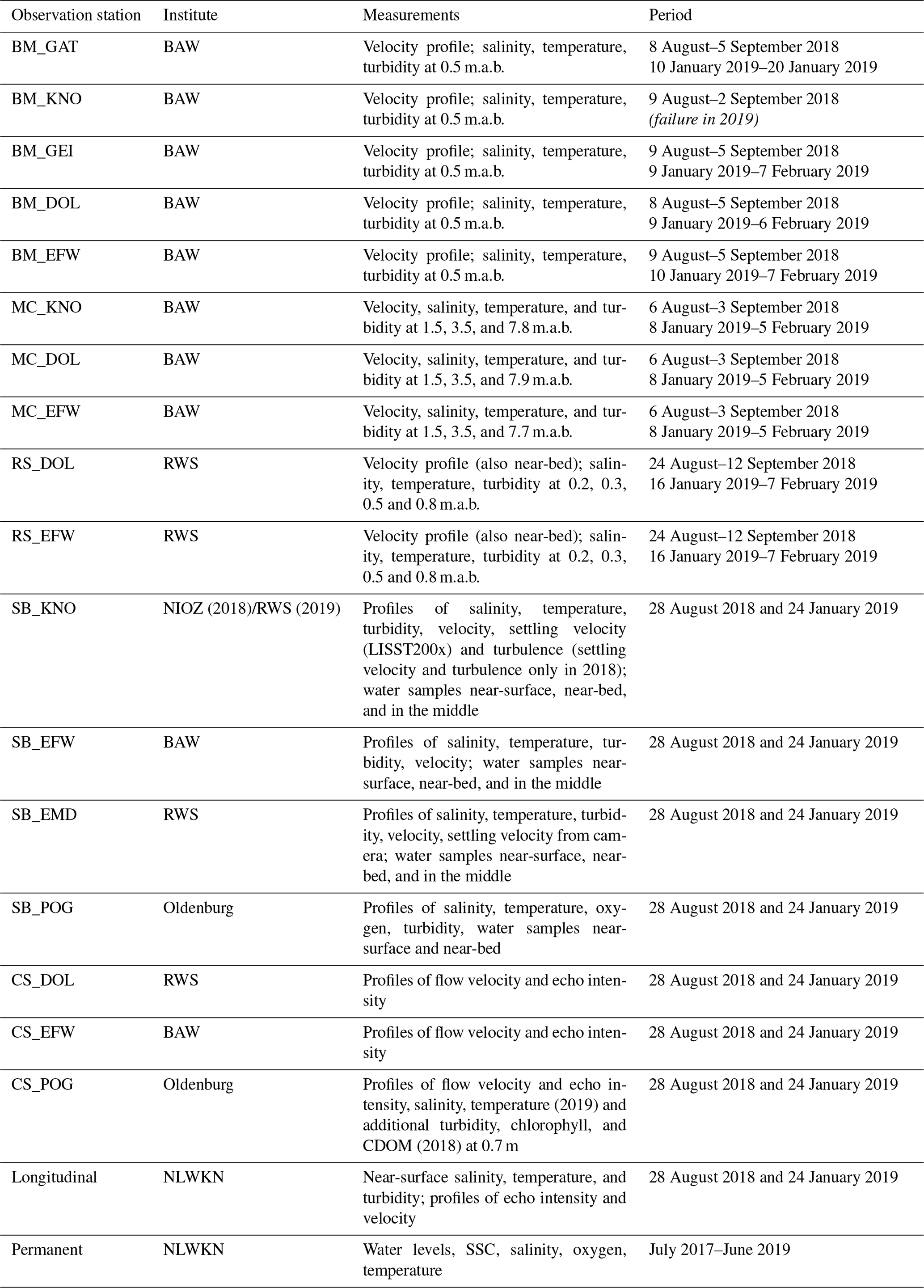
Observations covering at least one common spring–neap tidal cycle were executed at so-called bottom mounts (BMs), mooring chains (MCs), and larger bottom frames (RS) – see Table 1. In total, five bottom mounts, three mooring chains, and two larger frames were deployed throughout the study area (Fig. 1). The BMs were equipped with an upward-looking 600 mHz TRDI WH-S ADCP and a CTD with Seapoint STM turbidity sensor at 0.5 m.a.b. to measure salinity, turbidity, and temperature (Table 2); this vertical position allows ADCPs to measure the whole water column. The MCs measured salinity, turbidity, and flow velocity at a height of 1.5, 3.5, and 7.7–7.9 m.a.b. (depending on location, see Table 2) with the particular aim of detecting vertical gradients (especially salinity). The RS frames measured flow velocity throughout the water column by combining an upward-looking 600 mHz TRDI WH-S ADCP and a downward-looking high-resolution Nortek Aquadopp HR velocity profiler. Salinity, temperature, and turbidity were measured using OBS 3As deployed 0.2, 0.3, 0.5, and 0.8 m.a.b. in order to capture near-bed sediment transport processes. All ADCPs have an internal motion sensor and were installed in gimballed mounts to, automatically correct frame displacements (resulting from gravitational sliding or ship collision).

Figure 2 Definition of the measurement period of the 13 h surveys.

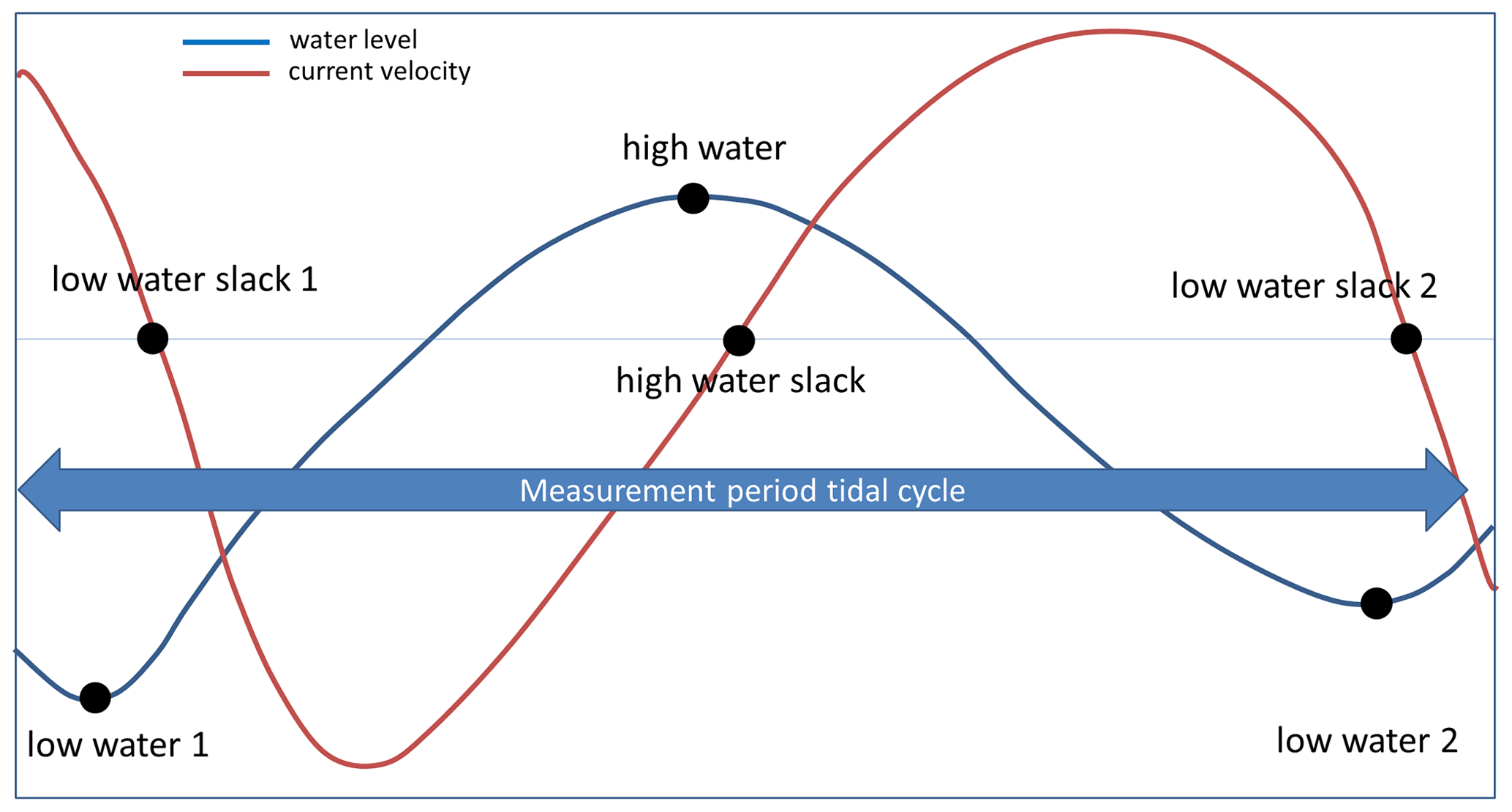
During each campaign, eight ships measured simultaneously in three different modes. Four ships were deployed in stationary mode, with SB_KNO, SB_EFW, and SB_EMD remaining anchored throughout the tidal period while SB_POG floated with the currents. All surveys started 30 min before local low water and ended 30 min after local high water (Fig. 2). Slack tide is close to high and low water in the Ems Estuary, and therefore the observations covered the period from the first to the second low water, but also from the first to the second low water slack.

All anchored ships measured the flow velocity with a downward-looking ADCP and temperature and salinity with a conductivity–temperature–depth (CTD) profiler equipped with an optical backscatter sensor (OBS). Water samples were taken at least once every hour at three water depths (near surface, near bed, and halfway down the water column, except for SB_POG which measured near bed and near surface only because of shallow waters) and analysed in the laboratory for suspended sediment mass. Water samples are, in general, important for conversion of turbidity (measured by the OBS) to SSC. However, with the high concentrations in the Ems Estuary, acoustic and optical instruments become progressively less reliable, making accurate water sampling an important source of data.

Additional instrumentation was deployed onboard the stationary boats at Emden (SB_EMD) and Knock (SB_KNO) to measure turbulence and sediment settling properties. At SB_EMD, hourly water samples were taken with a Niskin bottle close to the bed and close to the water surface. A subsample taken with a pipette (with an orifice approximately 6–7 mm in diameter, so large enough to not restrict large macroflocs passing through into the settling column) is inserted into a still and clear water settling column (with the same temperature and salinity as the in situ fluid) operated onboard, in which the water-sediment mixture settles from suspension. This extraction technique has been successfully utilized in numerous recent laboratory flocculation studies (e.g. Mory et al., 2002; Gratiot and Manning, 2004; Graham and Manning, 2007; Mietta et al., 2009) and creates minimal floc disruption during acquisition transfer to the column. Settling is monitored with a high-resolution video camera, and postprocessing of the camera data reveals the size, shape, and settling velocity of all particles registered with the camera. This provides a population of settling speeds and floc sizes, which can be averaged into a sample-averaged value (see e.g. Manning and Dyer, 2002). At SB_KNO, the settling properties were measured in August 2018 with a LISST200x in profiling mode using a high turbidity module. Turbulence was measured at the location of SB_EMD using a Rockland Scientific MicroCTD which was profiling the water column from a free-floating small vessel close to SB_EMD. The MicroCTD was used to collect measurements of turbulent kinetic energy (TKE) dissipation, as well as salinity, temperature, and turbidity data over 13 h transects during the summer (28 August 2018) and winter (24 January 2019) field campaigns. Data were collected in a series of vertical casts, with approximately five casts performed every 15 min. The five casts were averaged and bootstrapped 6000 times to provide a statistically significant measurement of TKE with depth (Efron and Gong, 1983; Huguenard et al., 2019; Ross et al., 2019, and references therein). Turbulence and flocculation properties were also measured at SB_KNO in August 2018 using an MSS-90-S microstructure profiler sampling at 1024 Hz. The profiler was used in free-fall mode with a downward velocity of approximately 0.6 m s⁻¹. The TKE dissipation rate was calculated by fitting the observed shear spectrum to the theoretical Nasmyth spectrum in a wave number range from 2 to a maximum of 30 cycles per metre.

Only flow velocities (measured with ADCPs) were measured at the cross-sectional profiles CS_DOL and CS_EFW, whereas salinity and temperature were additionally measured at CS_POG (using a towed FerryBox in 2018 and a CTD in 2019). The backscatter of the ADCP was calibrated to SSC using water samples and CTD profiles collected at nearby stationary boats. The CTD profiles were used to compute backscatter attenuation by salinity and temperature, thereby accounting for stratification effects. The residual backscatter was calibrated to SSC using the water samples. A longitudinal survey was carried out to measure near-surface salinity and SSC, sailing landward during the flood period (from Borkum on the island of Norderney to Papenburg close to the landward limit of the lower Ems River) and back during the following ebb period.

3.2 Data processing

All data were carefully examined for outliers and spikes were removed manually and through filters (velocity data). The acoustic Doppler velocimeter (ADV) and ADCP data were filtered using the signal-to-noise ratio of Elgar et al. (2005) and the 3D phase space method of Goring and Nikora (2002) and Mori et al. (2007) – see also van Prooijen et al. (2020). The deployment of OBS in all permanent stations and onboard SB_EFW and SB_EMD were calibrated in the laboratory in two steps. First, all the OBS outputs were individually calibrated to nautical turbidity units (NTU) using a milk suspension. Secondly, one of the sensors was additionally calibrated against SSC, and this NTU–SSC relation is applied to the other sensors as well. The data collected uniformly over all stations (velocity, salinity, SSC) were subsequently averaged to a 10 min time interval (and stored on a data repository). Additional datasets (concentrations and settling velocity from water samples, LISST data, turbulence data) are not averaged or averaged over a different time period or over a number of samples.

Additional data processing depends on the purpose of the data analyses. In this paper, we provide a synoptic view of residual flow and sediment transport, involving the conversion of point-observation data into fluxes. Residual fluxes can be computed from

• 13 h stationary ship observations (resolving the vertical variation in the flow velocity and SSC (based on OBS profiling), but lacking cross-sectional variation and resolving only a short period of time),

• 13 h transect observations (resolving the cross-sectional variation but using the ADCPs echo-intensity for SSC and resolving only a short period of time), and

• spring–neap observations using moored instruments (providing a much longer averaging period, but using near-bed OBS observations for SSC and lacking cross-sectional variation in the flow and SSC).

For reasons elaborated in Sect. 4, we will use the spring–neap observations to compute fluxes. For the RS and BM frames, the time-varying point fluxes F_p are defined as in Eq. (1):

$$\begin{array}{}\text{(1)}& F_{\mathrm{p}}=\overline{u}{c}_{\mathrm{b}}h,\end{array}$$

where $\overline{u}$ is the depth-averaged ADCP velocity profile, c_b is the concentration measured at 0.8 m (RS frames) or 0.5 m (BM frames), and h is the water depth. For the MC stations (measuring at three positions in the vertical), the average of the product of u and c (measured at height i) is multiplied with the water depth as in $F_{\mathrm{p}}=\frac{h}{\mathrm{3}}\sum _{i=\mathrm{1}}^{\mathrm{3}}{u}_i{c}_i$. For all observation locations, F_p is converted into a tide-averaged flux by integrating over a spring–neap tidal cycle (T=14.77 d), dividing by the number of M₂ tidal cycles N (with N=28.54), and multiplying with the channel width W:

$$\begin{array}{}\text{(2)}& F={\displaystyle \frac{W}{N}}\underset{\mathrm{0}}{\overset{T}{\int }}{F}_{\mathrm{p}}\left(t\right)\mathrm{d}t.\end{array}$$

We realize that this method has several shortcomings. Multiplying the depth-averaged velocity profile with a concentration measured at 0.6–0.8 m above the bed leads to an overestimation of the total flux. Additionally, multiplying a point measurement with the channel width ignores cross-channel variabilities in residual flow and SSC. We will revisit these shortcomings later in this paper.

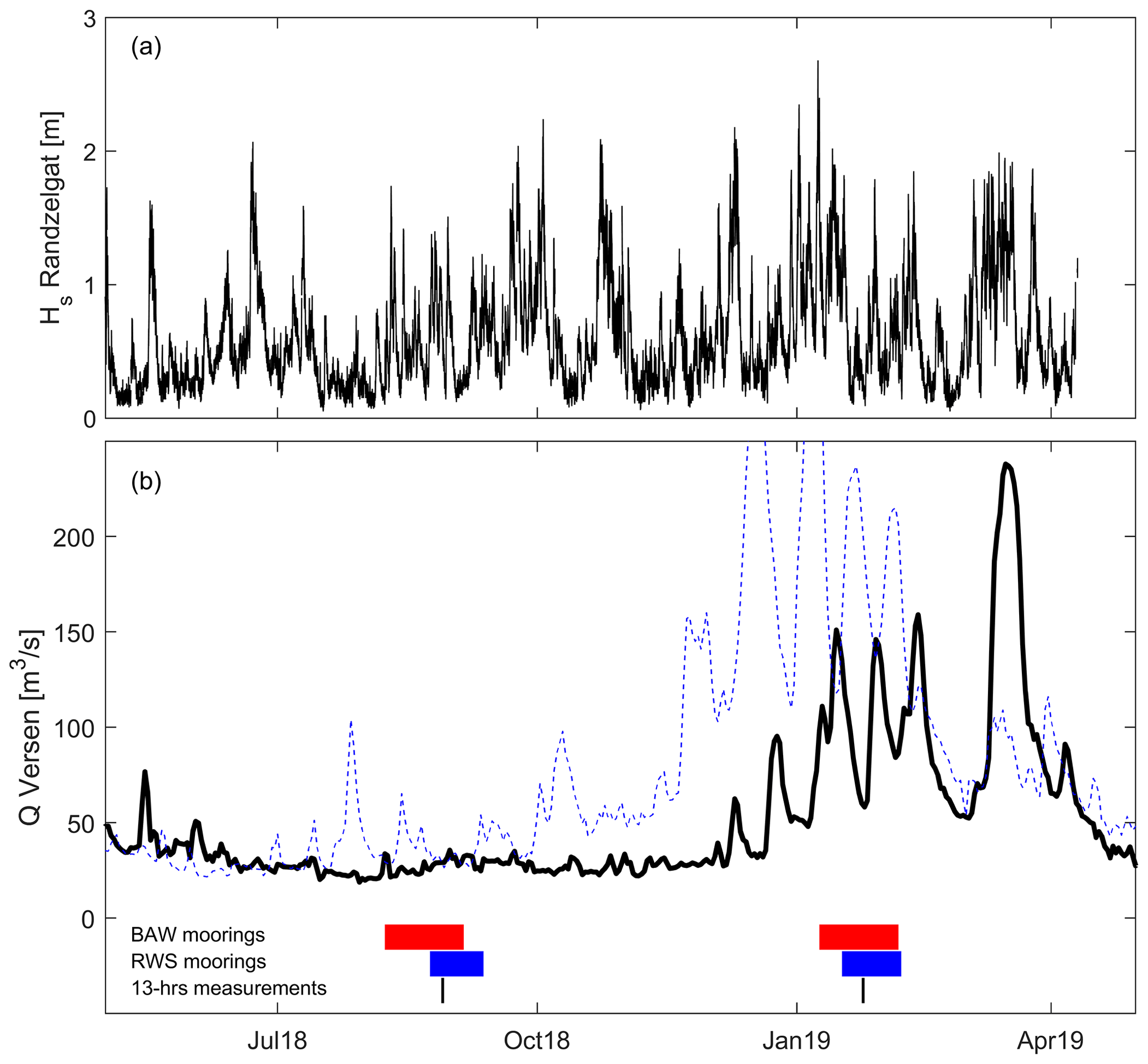
Figure 3 Wave height H_s measured at station Randzelgat Noord (a) and discharge of the Ems River at Versen (b) from 1 May 2018 to 1 May 2019, with deployment dates of BAW frames, RWS frames, and the 13 h measurements added to (b). The dashed blue discharge in (b) is the discharge of the period 1 May 2017 to 1 May 2018.

3.3 Environmental conditions

The 2018 surveys were characterized by low wind speed, wave height, and river discharge, i.e. representing tide-only conditions (Fig. 3) – see also Schulz et al. (2020). The river discharge during the 2019 surveys was higher than in 2018, although rather low for winter conditions. The first high river discharge peaks occurred relatively late in the season, with the 13 h measurements between two high-discharge events. Exact discharge conditions at the survey location is not known, as the discharge is measured >100 km upstream of the weir at Herbrum (resulting in a delay and flattening of the river discharge peak). Offshore wave conditions were slightly higher in winter than in summer, without prominent storm conditions.

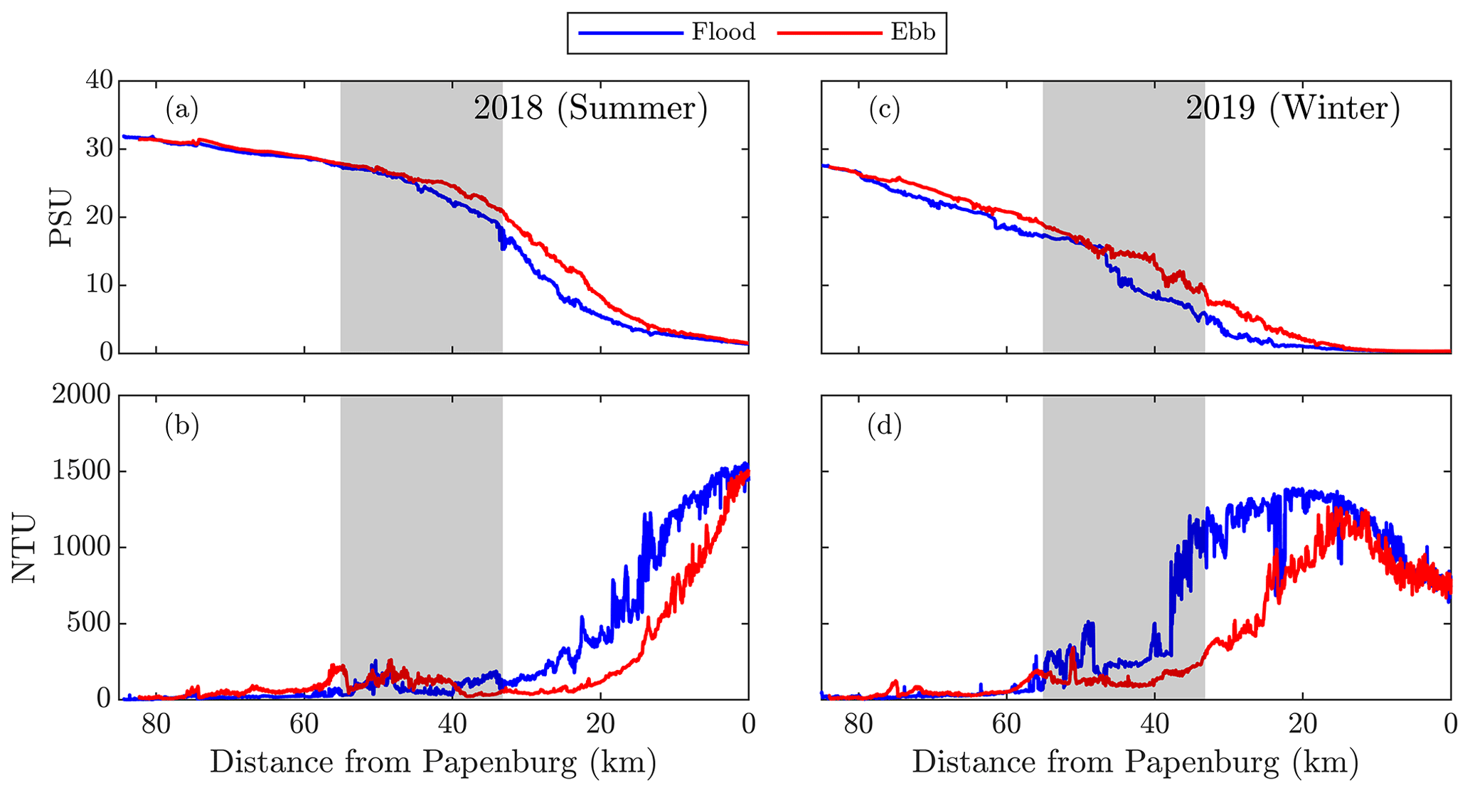
Figure 4 Longitudinal near-surface salinity (a, c, in PSU) and turbidity (b, d, in NTU) distribution observed in 2018 (a, c) and 2019 (b, d), during the flood (blue) and during the ebb (red) cruise. The survey starts at 85 km (Borkum) at the beginning of the flood and reaches Papenburg around the transition from flood to ebb after which it sails back for 6 h with the ebbing tide. The grey-shaded area denotes the focus area of the EDoM campaign. Observations were made with a near-surface sensor towed by the ship, and therefore no near-bed observations are available.

The difference in discharge conditions resulted in a markedly different salt intrusion and location of the estuarine turbidity maximum (ETM) (Fig. 4). In summer, the salinity in the fairway to Emden (grey-shaded area in Fig. 4a) is between 20 and 27 ppt, and the ETM is completely located in the lower Ems River (Fig. 4b). During winter conditions, the salinity in the fairway is between 5 and 20 ppt (Fig. 4c). The ETM has shifted 25 km in the seaward direction and is partly located in the fairway to Emden (Fig. 4d).

4 Results

4.1 Data collection

The majority of instrumentation worked well, with the following exceptions. The NTU values of the various OBS instruments were within 5 % of each other, except for one which is subsequently discarded from the dataset. The frame BM_KNO malfunctioned in 2019 for the complete period, while frame BM_GAT only collected data in the first 10 d of the 2019 deployment (see also Table 2). Frame BM_GAT also malfunctioned during the last 3 d of its 2018 deployment. LISST measurements onboard SB_KNO failed in both 2018 and 2019, and have therefore been excluded from this paper. No measurement errors resulting from sliding, slumping, or boat accidents have been identified, and no biofouling was detected upon retrieval of the frames. The accuracy of the various instruments has not been investigated as part of this specific measurement campaign. However, decades of experiments with similar surveys, including dedicated accuracy tests, suggest that the accuracy of flow velocity observations is within 1 %, discharges (using ADCP cross-section surveys) are within 5 %, and SSC is within 10 % (using OBS) to 20 % (using ADCP). The accuracy of concentration measurements depends on the range of the sediment concentration, typically being lowest at very low or high SSC.

The high SSC values only negatively influenced the ADCP measurements at the Pogum location (where concentrations were up to several kg m⁻³), which where therefore considered unreliable in both 2018 and 2019 (and therefore excluded from further processing). Other velocity measurements were not negatively impacted by high SSC values because of the deployment of low-frequency ADCPs in areas with high SSC. The OBS calibration revealed that the SSC increase is slightly nonlinear with output voltage within the general range of SSC occurring in the study site (mostly up to several kg m⁻³) and therefore calibrated with a power function. The calibration remains linear to slightly non-linear up to 8 kg m⁻³; at higher SSC values the OBS output becomes unreliable. Such concentrations were only encountered at Pogum (or very infrequently at other locations). The point at which the output voltage starts decreasing with increasing SSC (as is common for optical instruments) was not been reached during the field surveys.

We will highlight some of the key observations made during the EDoM campaigns illustrating the synoptic nature of the observations in a complex 3D flow environment with high suspended sediment concentrations, by examining residual flows and transport in more detail in the following sections (Sect. 4.2 and 4.3) using velocity and ADCP observations. Additional turbulence data were collected at SB_KNO (August 2018 only) and at SB_EMD (both campaigns). The SB_KNO turbulence data provide insight in mixing and stratification processes in response to lateral and longitudinal flows (Schulz et al., 2020), whereas the SB_EMD data reveal how sediment-induced stratification processes may promote ebb-dominant sediment transport (Bailey et al., 2022). The floc size measurements reveal a large variability in settling velocity within a tidal cycle (with higher settling velocities during the flood than during the ebb) but also a large seasonal variability: the settling velocity was higher during the August observations than during the January observations. Such a tidal variability may influence residual transport of sediment (promoting ebb transport) whereas the seasonal variation probably influences the seasonal variation in dredging (higher in the summer period).

Figure 5 Residual flow velocity near the surface (a, b) and near the bed (c, d) over the 13 h measurement period on 28 August 2018 (a, b) and 24 January 2019 (c, d), including moorings (BM_GEI, RS_EFW, RS_DOL, BM_DOL, MC_DOL), shipborne stationary observations (SB_EFW) and the transects in the Fairway to Emden (CS_EFW) and in the Dollard (CS_DOL).

4.2 Residual flows

Horizontal residual flows can be computed from the frames, stationary boats, and from boats sailing in transects. Figure 5 displays the tide-averaged residual flow from the 13 h stations as well as the longer moored instruments near the surface and near the bed on 28 August 2018 and 24 January 2019. The combined point and transect observations reveal a consistent pattern of residual flows. In the mouth of the Dollard, the transect data reveal cross-sectionally varying residual flows, especially near the surface, but averaged over the cross-section there is no preferential inflow or outflow. Hence the moored observation stations in the Dollard (BM_DOL and MC_DOL) represent the flows through the mouth of the Dollard. Station RS_DOL reveals net outflow (both near the surface and near the bed), probably resulting from local bathymetric constraints.

In the mouth of the fairway to Emden a pronounced cross-channel and vertical stratification pattern exists during both low (Fig. 5a and c) and high-discharge conditions (Fig. 5b and d). The surface flow velocities are directed seawards (Fig. 5a and b), whereas the near-bed currents are directed landwards (Fig. 5b and d). On top of this, a pronounced south to north gradient exists, with prevailing landward residual flow in the south and seaward flow in the north. Apparently, the velocities in the moored stations in the north are slightly seaward-directed, while those in the south are more landward-directed. This pattern will be elaborated in more detail hereafter.

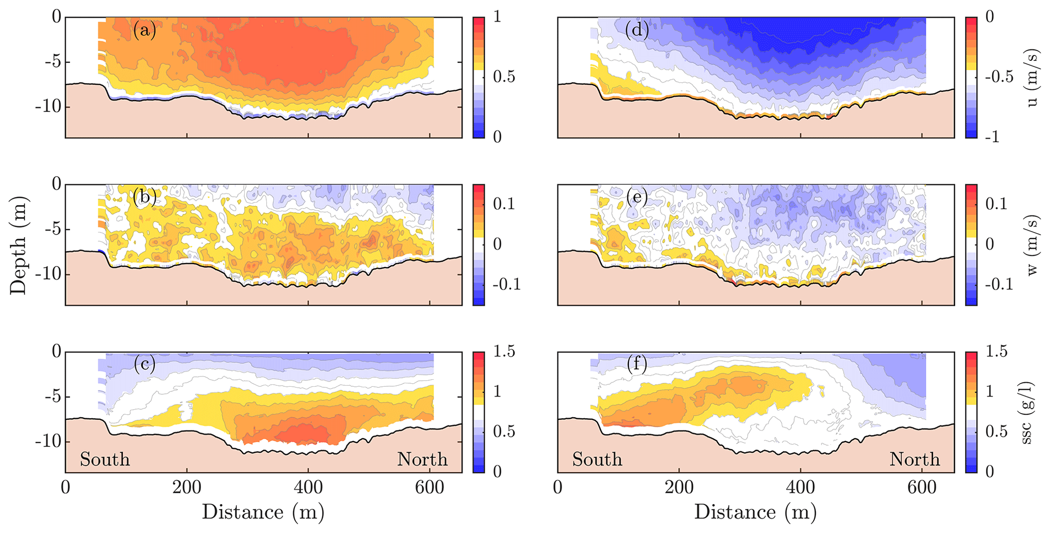
Figure 6 Velocity and SSC measured at CS_EFW cross-section in 2019 averaged over the flood (a–c) and ebb (d–f). (a, d) measured along-channel current velocities; (b, d) cross-channel current velocities (northward positive) and (e, f) SSC based on ADCP backscatter conversion.

During the ebb, the along-channel flow velocities are much larger along the northern outer bend of the ENC (cross-section CS_EFW in Fig. 6d); we attribute this to bathymetric constraints imposed by the curved channel. During the flood, however, the flow is much more cross-sectionally uniform. Averaged over the tidal cycle, this leads to outflow along the northern bend and inflow along the southern bend (see cross-section CS_EFW and station RS_EFW in Fig. 5). This cross-sectional variation of the along-channel flow velocity also gives rise to a transverse flow pattern with a northward-directed bottom current during both the ebb and the flood (Fig. 6b and e), compensated for by a southward flow near the surface. A curvature-induced secondary flow would lead to a near-bed flow from the outer bend to the inner bend, i.e. towards the south during both the ebb and flood. The northward near-bed flow can be explained, however, by the lateral advection of the salinity gradient. During the ebb, the cross-sectional variation of the flow leads to a lower salinity along the northern bend compared to the southern bend. This positive salinity gradient from north to south drives a classic gravitational flow with northward flow near the bed and southward flow near the surface. During the following flood phase, this cross-sectional salinity gradient is largely maintained because the flood currents are cross-sectionally uniform. Therefore, the near-bed transverse currents remain directed towards the north (and towards the south near the surface).

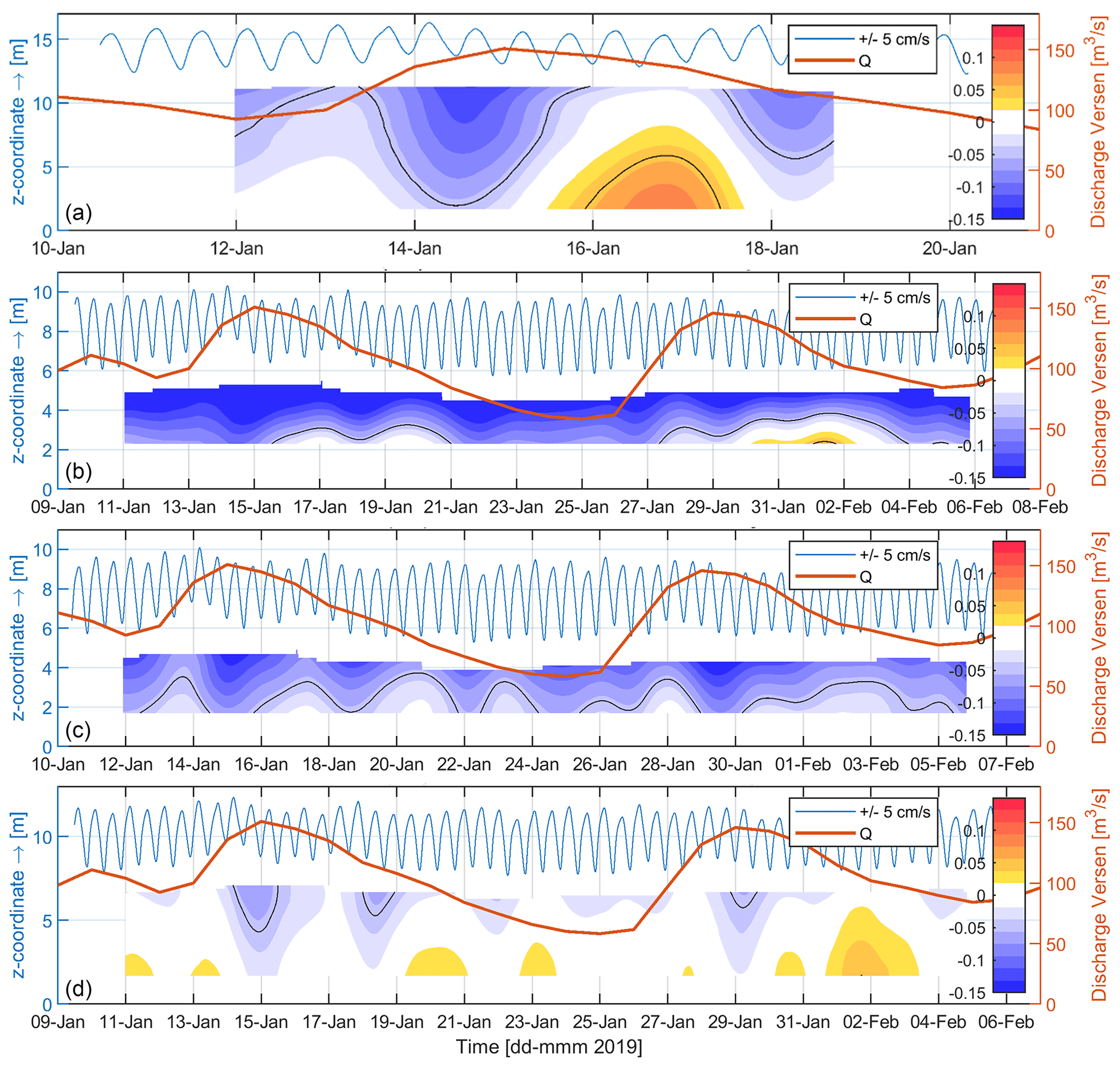
Figure 7 Godin-filtered residual longitudinal flows (landwards positive) measured with the bottom mounts (BMs) at stations GAT (a), GEI (b), EFW (c) and DOL (d) in 2019. A Godin low-pass filter removes tidal flow velocities from the observation, showing temporal variations of the average flow velocity.

Stratified flows exist not only perpendicular to the main flow direction (as shown in Fig. 6) but also in the along-channel direction. These along-channel residual flows are revealed by low-pass filtering the along-channel flow (Fig. 7). All stations reveal a seaward-directed residual surface current during periods of high river discharge, and a landward-directed near-bed current during the waning stage of the river discharge peak. This discharge dependency appears to be weaker for stations within the ENC (GEI and EFW) than for those in the Dollard and outer Ems Estuary (DOL and KNO). Such near-bed flows are important for residual sediment transport (as typically most sediment transport takes place close to the bed), but unfortunately the lowest 2 m of the water column is not measured with the upward-looking ADCPs. It is therefore likely that landward flows are more strongly developed than suggested by Fig. 7.

4.3 Residual sediment transport

The residual sediment transport can be computed with the transect observations, the moored 13 h stations, and the moored instruments (see Sect. 3.4). Figure 7 reveals that the subtidal flows are substantially varying, especially during the January surveys, in response to river discharge fluctuations. This discharge variability not only influences the hydrodynamics but also the supply of sediments from the lower Ems River (with a high river discharge flushing sediments seawards). Because of this variability, the 13 h surveys may not represent typical conditions (especially during the winter observations). We therefore present residual fluxes using the moored instruments (Fig. 8) measuring a spring–neap tidal cycle.

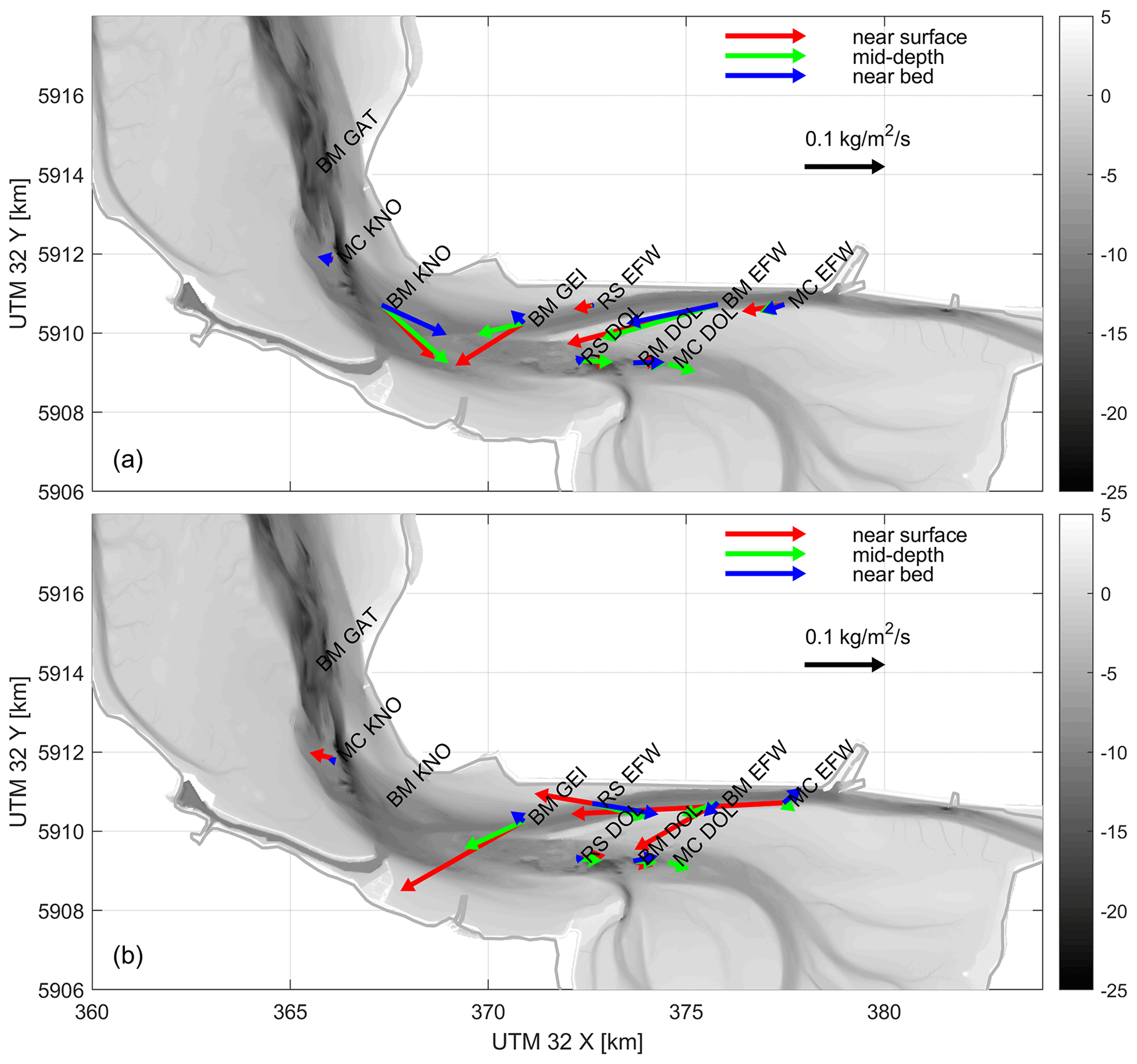
Figure 8 Residual sediment transports (kg m⁻² s⁻¹) computed at all observation stations with a length exceeding the duration of a spring–neap cycle in 2018 (a) and 2019 (b) for which velocity and SSC observations are available. At MC stations, velocities at three positions in the vertical are multiplied with SSC at the same position. At other locations, velocity profiles as collected by an ADCP are multiplied with near-bed SSC.

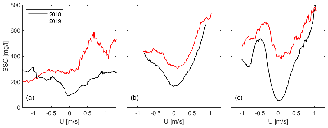
Figure 9 Sediment concentration averaged per eastward flow velocity U (flood currents positive) over a spring–neap tidal cycle for the moored observations in the Dollard: RS_DOL (a), MC_DOL (b), and RM_DOL (c).

The computed fluxes using all moored instruments provide a spatially, temporally, and vertically consistent picture. The three Dollard moorings yield fluxes in the same direction but even of comparable magnitude within each campaign and between campaigns. These observations strongly suggest the Dollard is importing sediments. The residual fluxes are not the result of residual flows (Fig. 5) but of an asymmetric availability of sediments (Fig. 9). The SSC is higher during the flood than during the ebb, probably at least partly consisting of sediment that was discharged into the outer Ems Estuary from the lower Ems River during the previous ebb phase.

The fluxes in the ENC are directed seaward, during both low and high-discharge conditions, and on both the north bank (BM_GEI, RS_EFW) and south bank (BM_EFW and MC_EFW). The latter is important given the cross-sectional variability in longitudinal flows (Fig. 6): apparently the residual transport is directed seaward despite periods with landward-directed residual flows. The seasonal coherence in residual fluxes is surprising, especially given the salinity-driven landward currents in response to periods with higher river discharge revealed in Fig. 7. The higher river discharge in January does lead to a larger difference between near-bed and near-surface transport: in general, the (seaward-directed) surface sediment fluxes are larger in January than in August while the near-bed fluxes are weaker (or even landward-directed, as for RS_EFW).

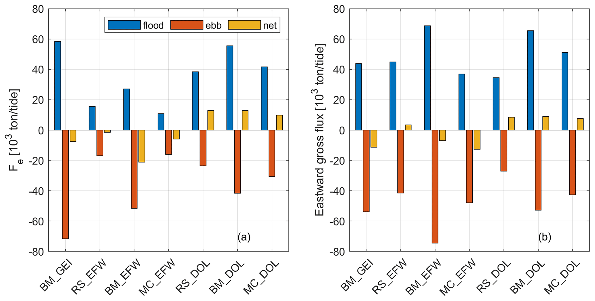
Figure 10 Gross and net flux F_e (eastward positive), computed from one spring–neap cycle of observations at the long-term moorings in 2018 (a) and 2019 (b).

The consistency of the computed sediment fluxes is further supported by an evaluation of the gross and net sediment fluxes (Fig. 10). Systematic differences between ebb and flood fluxes may easily arise from bathymetric constraints (the measurement location is in a flood or ebb-dominant location) or measurement shortcoming (a slightly different sediment type during ebb or flood leads to differences in ebb and flood concentrations due to the dependence of sensors to the sediment grain size). A net sediment flux of e.g. 1 % may then reverse direction with a 2 % error in the gross fluxes. However, in the Dollard, the residual flux is approximately 20 % of the gross flux. Such a large net flux (relative to the gross flux) makes it relatively insensitive to measurement shortcomings. In the ENC, the ratio of net to gross fluxes is more variable (between several percent at RS_EFW and 40 % at BM_EFW) but overall, typically more than 10 %. This also suggests that the fluxes in the fairway to Emden are fairly accurate.

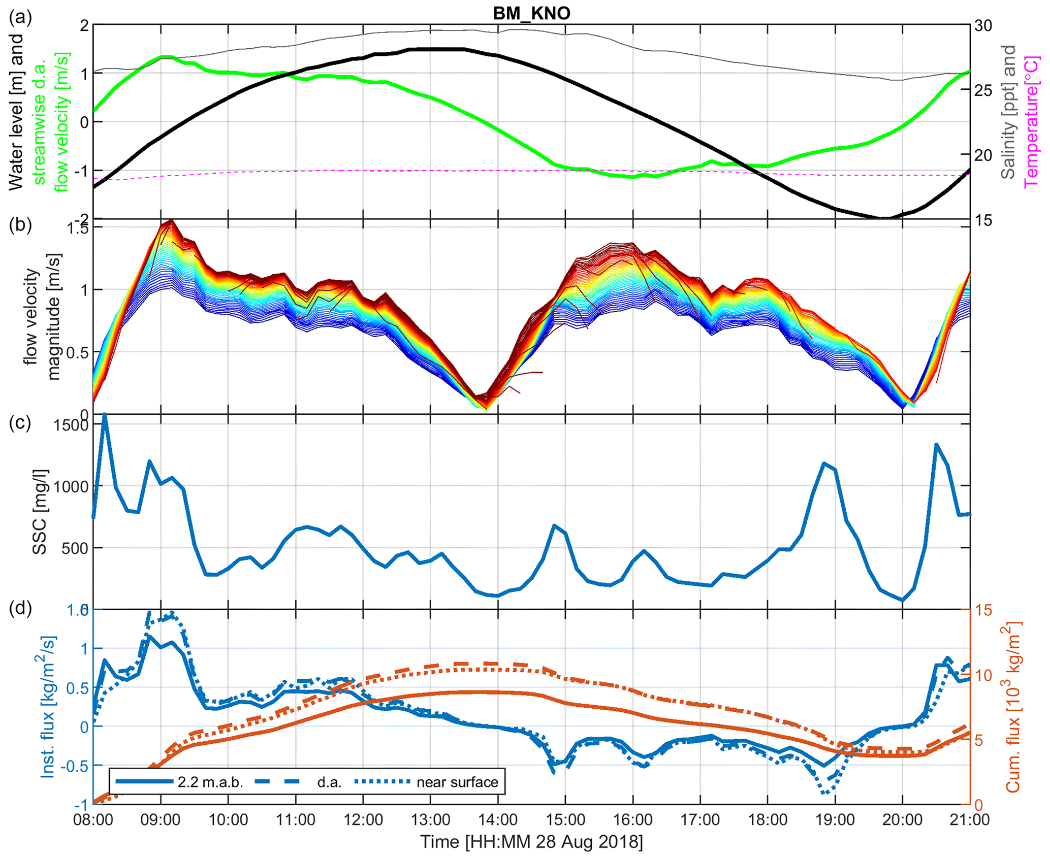
Figure 11 Tidal cycle observations at Knock (BM_KNO), showing the water level (black), salinity (grey), depth-averaged flow velocity (green) and temperature (pink, a), the depth-varying flow velocity (red near the surface, blue near the bed, b), the sediment concentration near the bed (c), and instantaneous and cumulative sediment flux (landwards positive; d).

Station BM_KNO reveals a pronounced landward residual transport in August but was unfortunately malfunctioning in January (Fig. 8). This residual sediment transport is in agreement with large up-estuary transport illustrated with the dredging volumes in the ENC and lower Ems River as well as the hyper-turbid conditions in the lower Ems River. This landward transport results from a phase difference between maximal flow velocity and maximal sediment concentration, illustrated in Fig. 11. The first half of the flood is characterized by a faster rise of water levels compared to the second half, whereas the falling stage is much more uniform – the duration of rising and falling water levels is the same (Fig. 11a). As a result, (1) the flood flow velocities are maximal at the beginning of flood, whereas ebb flow velocities are maximal later in the ebb and (2) the flood velocity peaks are slightly higher than the ebb velocity peaks (Fig. 11b). Although depicted here for station BM_KNO, this asymmetry in velocity peak phasing is observed throughout the various observation stations, although in some stations, ebb flow velocities are higher. An asymmetry with a different duration of the period of high water slack compared to low water slack is known as slack duration asymmetry (Friedrichs, 2011). A longer duration of high water slack (as at station BM_KNO) is typical for high water duration asymmetry, with a water level phase difference θ_ζ between the M2 and M4 tidal constituents ${\mathit{\theta }}_{\mathit{\zeta }}=\mathrm{2}{\mathit{\varphi }}_{{\mathit{\xi }}_{\mathrm{M}\mathrm{2}}}-{\mathit{\varphi }}_{{\mathit{\varsigma }}_{\mathrm{M}\mathrm{4}}}$ between 90 and 270^∘ (and maximal at 180^∘). This is supported by long-term water level observations collected at Pogum, of which tidal analysis reveals a value for θ_ζ very close to 180^∘ (van Maren et al., 2015b).

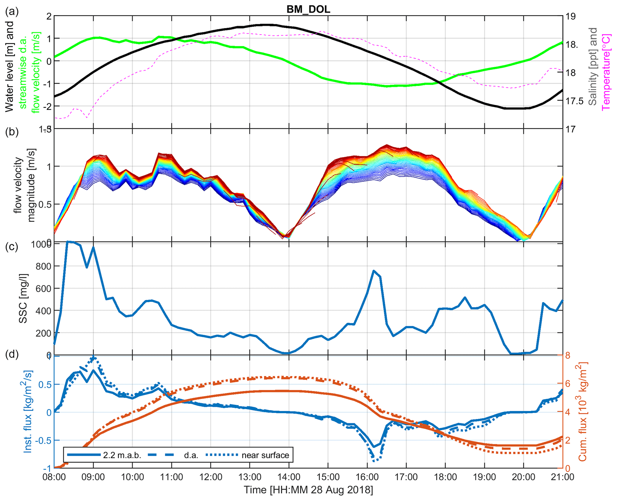
Figure 12 Tidal cycle observations at the mouth of the Dollard (BM_DOL), showing the water level (black), salinity (grey), depth-averaged flow velocity (green), and temperature (pink, a), the depth-varying flow velocity (red near the surface, blue near the bed, b), the sediment concentration near the bed (c), and instantaneous and cumulative sediment flux (landwards positive; d).

The observed tidal asymmetry in SSC (Fig. 11c) is primarily reflecting advection of sediment flowing out of the ENC at the end of the ebb (18:00–20:00 UTC) which is after flow reversal transported back into the ENC (20:00–21:00 and 08:00–10:00). However, during the flood, a second SSC peak exists (from 08:30 to 09:30), superimposed on the advection peak and corresponding to the flow velocity peaks. The cumulative sediment fluxes (Fig. 11d) show that this phase (where a period of high SSC coincides with a period of high flow velocity) has a major influence on the residual sediment transport. Apparently, the early peak in the flood flow velocity (resulting from high water duration asymmetry) is important for the residual transport of sediment. The observed residual transport in Fig. 11 is also representative for a longer period of time: the computed cumulative flux of 5×10³ kg m⁻² over the tidal cycle corresponds to 0.11 kg m⁻² s⁻¹, which is very close to the average flux computed over a spring–neap tidal cycle (Fig. 8). Spatially, however, the direction of residual fluxes is more variable. Transport is ebb-dominant in station SB_KNO (see Schulz et al., 2020), located 1 km southeast of BM_KNO. This difference may reflect lateral variability in the plume flowing out of the lower Ems River, directly crossing location SB_KNO during the ebb but then deflecting northward to travel past location BM_KNO during the flood.

The observations in the mouth of the Dollard show a remarkable similarity with those collected at Knock (Fig. 12). The flood flow velocities peak at the beginning of the flood which, combined with the high SSC during this period, results in a large landward-directed sediment flux. It seems likely, however, that the large SSC peak measured at the beginning of the flood is especially large in the mouth of the Dollard because turbid water that was discharged from the ENC during the previous ebb flows into the Dollard with the incoming flood currents. Despite the large landward sediment flux (10×10³ t tide corresponding to 7×10⁶ t yr⁻¹), bathymetric data records reveal that there is no net accumulation of sediment in the Dollard. Apparently, sediment must also flow out of the Dollard – this will be discussed in Sect. 5.

High water duration asymmetry provides a mechanism transporting sediment into the outer estuary (and partly into the Dollard), but this asymmetry is insufficient to explain the large sediment flux towards the lower Ems River. The strongest evidence for mechanisms driving transport from the ENC to the lower Ems River is provided by water samples collected at the beginning of the ENC (SB_EFW), halfway into the ENC (SB_EMD), and within the lower Ems River (SB_POG). Water samples provide an important methodology to measure the sediment concentrations in the ENC because of the high SSC (up to 35 kg m⁻³, which is beyond the detection limit of many optic and acoustic instruments), and because of technical difficulties with the POG observations. Simply comparing the SSC concentration of these three stations throughout the 13 h tidal cycle sampled in January 2019 reveals a progressive increase in near-bed SSC during the flood from <1 kg m⁻³ (EFW) to ∼15 kg m⁻³ (EMD) to ∼30 kg m⁻³ (POG). This spatial trajectory is within the tidal excursion (<15 km) and therefore the most likely explanation of this landward increase in SSC is sediment resuspension from the bed. The origin of this sediment will be discussed in more detail in the following section. The concentration is much lower during the following ebb (∼10 kg m⁻³), suggesting that the sediments transported landward during the flood have deposited in the lower Ems River. Interestingly, during this period of apparent strong sediment import, the salinity profiles were reversed (with lower salinity values near the bed than near the surface), suggesting partly decoupled flow dynamics in the highly concentrated layers near the bed from the water masses higher in the water column (as has been described for the fluid mud reach in the lower Ems River by Becker et al., 2018).

5 Main findings and future work

The three research questions that motivated this study where related to the mechanisms for upstream sediment transport, the impact of high SSC in the lower Ems River on the outer estuary, and the high maintenance dredging rates in the ENC. This EDoM campaign has provided important new insights into the mechanisms regulating exchange of water and sediment between the lower Ems River and its outer estuary. At the same time, these new insights have also raised new questions that need to be addressed, partly through more detailed analyses of the collected data. We will first address the main questions motivating the measurement campaign, followed by potential follow-up studies using the collected data.

5.1 Sediment dynamics

5.1.1 Landward sediment transport mechanisms

One of the motivations for the EDoM campaign was to understand the mechanisms leading to landward transport in the ENC because known mechanisms (tidal asymmetry, salinity-induced estuarine circulation) appeared to be too weak to explain the large landward transport. Surprisingly, the field observations suggest that the ENC is exporting. It is therefore hypothesized that a large-scale horizontal circulation exists where sediment flows into the Dollard and flows back into the ENC during either fair-weather conditions or during storm conditions. A substantial residual flow over the Geise dam from the Dollard to the ENC has indeed been observed (Jensen et al., 2002). However, subsequent observations carried out to further validate this (not reported here) have not yet confirmed this residual transport due to higher SSC in the ENC than in the Dollard. The role of the Dollard, and the closure of the mass balance in the Ems Estuary (Fig. 8) is therefore still not completely resolved.

Based on single station observations, the main mechanism responsible for the sediment transport towards the ENC and the Dollard appears to be slack water duration asymmetry. Further landward spatial asymmetries become progressively more important. Transport is directed towards the Dollard because of the high SSC at the beginning of the flood, which can be traced back to outflow of turbid water from the ENC but also explained by (high water) slack water duration asymmetry. However, the concentration peak at the beginning of the flood (leading to overall flood-dominant transport during calm conditions) was already observed in 1996 (Dyer et al., 2000) when the lower Ems River was not as turbid as it is nowadays. This suggests that transport into the Dollard is primarily driven by high water slack duration asymmetry, strengthened by outflow of turbid water from the ENC.

Net transport from the ENC into the lower Ems River is not driven by an asymmetry in the flow, but by sediment availability. The large role of sediment availability is demonstrated by the steep increase of the landward sediment flux throughout the ENC (Fig. 13). This large sediment availability may reflect sediment transport from the outer Ems Estuary via the Dollard, over the Geise dam into the ENC (as discussed above). Alternatively, the large up-river sediment flux may be the result of large sediment deposits during a high-discharge event that occurred several days before the 13 h observations (Fig. 7).

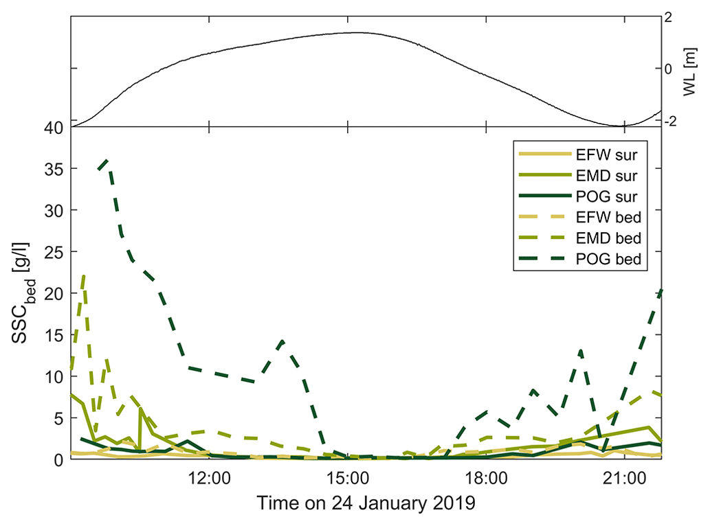
Figure 13 SSC based on water samples collected in the Fairway to Emden (station SB_EFW and SB_EMD) and the lower Ems River (SB_POG) on 24 January 2019 near the bed (top) and near the surface (bottom).

5.1.2 Impact of high SSC in the lower Ems River on the outer Ems Estuary

Prior to the measurement campaign, sediment was believed to be transported up-estuary (through the ENC to the lower Ems River) during low-discharge conditions, being flushed out again during periods of higher river discharge (Spingat and Oumeraci, 2000; van Maren et al., 2015b). The outer Ems Estuary may therefore be more strongly impacted during high-discharge conditions. In addition to the river discharge, the high sediment concentrations in the lower Ems River permanently increase the sediment concentration in the downstream outer estuary by shear dispersion.

The collected dataset suggests that a number of mechanisms exist that reduce the effect of the lower Ems River on the outer Ems Estuary. First, high-discharge events are immediately followed by a phase of intensified gravitational circulation, with a landward-directed current transporting sediment that settled from suspension after the period of higher discharge back towards the ENC. Secondly, the asymmetry of tidal currents (with a high flow velocity at the beginning of flood) suggests that turbid water flowing out of the ENC is effectively transported landward. Thirdly, the sediment-rich water flowing out of the ENC is diverted back into the Dollard, from which the sediment is hypothesized to flow back into the ENC over the Geise dam. On the other hand, two mechanisms have been identified which could raise SSC in the outer Ems Estuary due to the high turbidity in the lower Ems River. First, the sediment transport in the ENC is directed seaward, providing a permanent conduit for sediment to be transported from the lower Ems River into the outer Ems Estuary. Secondly, part of the turbid water flowing out of the ENC directly flows into the Dollard after reversal of the tides. This would suggest a steady increase in SSC in the Dollard in response to the increasing SSC in the lower Ems River, which is in line with observations (van Maren et al., 2015a). Determining which of the mechanisms above is stronger, and hence to what extent flushing of the lower Ems River influences the turbidity in the outer Ems Estuary, requires additional modelling. The EDoM dataset provides new insights on processes to resolve in such models as well as observations to calibrate the models with.

5.1.3 Large maintenance dredging rates

The computed sediment fluxes suggest convergence of sediment transport at the mouth of the ENC, which is exactly the location where most maintenance dredging is taking place. Prior to the measurement campaign, the reasons for this location where poorly understood, as the ENC was considered to be transporting sediment from the outer Ems Estuary towards the lower Ems River. However, the seaward sediment transport suggested by the moored observations provide a good explanation for the location and the magnitude of the maintenance dredging rates. Based on a preliminary analysis of the collected data, the convergence of sediment transport appears to be the result of a balance between (1) high water slack asymmetry (driving a landward transport in the estuary) and (2) the high concentration gradient and a seaward-directed residual flow in the ENC (driving the seaward sediment flux).

5.2 Future work

The EDoM measurement campaign provided important new insights into sediment dynamics, but also exposed gaps in knowledge that may be filled in by additional analyses of the collected data. Within the scope of the original project, we provide the following directions for future research using the collected dataset.

• The collected synoptic dataset has substantially increased our understanding of exchange mechanisms between the outer Ems Estuary and the lower Ems River. However, the relative importance of these mechanisms on exchange, including their seasonal variability, still remains to be quantified in more detail. A way forward here is to decompose the sediment fluxes into tidal pumping, advection, and estuarine circulation terms (following e.g. Dyer, 1988).

• The computed point sediment fluxes provide a consistent picture of the residual transport, but their accuracy could be improved because of the assumption made to vertically and cross-sectionally extrapolate the data. The cross-sectional variation of the flow (as measured at the transects) and the vertical distribution of SSC (measured with the stationary boat surveys) provide means to better extrapolate the fluxes over depth and the channel cross-section.

• The measurements in the Dollard and ENC suggest that a horizontal residual transport cell (with sediment transport towards the Dollard and via the Geise dam into the ENC) exists, but this circulation has not yet been supported by an equivalent transport magnitude over the dam based on field data. It is recommended to further investigate this circulation pattern through a combination of modelling work, collection of new data, and/or re-analysis of the sediment fluxes (as described above).

• Slack water duration asymmetry appears to be an important mechanism transporting sediment landward in the outer Ems Estuary. Its importance for residual landward transport should be investigated in more detail through systematic tidal analyses of water levels and flow velocity, and the intra-tidal relation between currents and SSC.

• A first analysis of the flocculation data (not shown here) has indicated that the intra-tidal and seasonal variability in the settling velocity is large and may contribute to sediment deposition in the ENC, and therefore the seasonal variation in maintenance dredging volumes.

• The sediment concentration gradients in the ENC were sufficiently large to influence turbulent mixing, and thereby sediment dynamics and residual transport. The collected data suggest that sediment-induced turbulence damping weakens sediment transport in the flood direction (Bailey et al., 2022).

• The cross-sectional data revealed pronounced transverse flows in the ENC despite its limited width (∼500 m). The collected data, with frame and shipborne measurements on both sides of the channel provide information to determine the lateral and longitudinal density gradients driving these complex flow patterns. It is recommended to investigate these lateral flows in greater detail, including its role on residual sediment transport.

• Based on data only, it is not yet feasible to exactly quantify the role of the lower Ems River on the turbidity in the outer Ems Estuary. The impact of sediment flushing from the lower Ems River and the ENC on turbidity in the outer Ems Estuary requires detailed further analysis of the data (for instance through decomposition of fluxes, as above) in combination with numerical modelling (for which the EDoM data provide valuable calibration data).

• Regarding the exchange of sediments between the lower Ems River and the ENC, i.e. upstream transport versus downstream flushing, the region of the highest along-channel sediment-induced density gradient downstream of the fluid mud reach is critical in understanding the Ems system, but was not part of the EDoM survey. It is recommended to complement the EDoM dataset by conducting new measurements in this part of the channel, upstream of Pogum and including the downstream part of the fluid mud reach.

These recommendations are site-specific, and some of these recommendations will be part of future research executed by the project partners. Nevertheless, we also invite researchers outside the project team to contribute to our understanding of sediment dynamics in the Ems Estuary. In addition to the site-specific data analysis directions provided above, the collected dataset also has the potential to advance our knowledge on the following:

• near-bed fine sediment dynamics measured with the RS_DOL and RS_EFW frames; turbidity sensors were placed at 0.2, 0.3, 0.5 and 0.8 m above the bed providing valuable information, together with hydrodynamics (a downward-looking Aquadopp and near-bed ADV sensors) on near-bed fine sediment dynamics in turbid environments (which are limitedly understood – see van Maren et al., 2020),

• the use of optical and acoustic instruments for measuring SSC in high concentration environments, by comparing SSC values based on ADCP, OBS and water sample observations,

• Transverse flows and sediment transport patterns resulting from topographic constraints and density differences (joint analysis of the various mooring data, shipborne moored observations and transect data collected in the ENC).

6 Data availability

Most data collected during the EDoM field campaign are stored on the repository of 4TU: https://doi.org/10.4121/c.6056564.v3 (van Maren et al., 2022). Most data stored on the repository are averaged at 10 min intervals; water sample, settling velocity, and turbulence data are stored at different intervals. All data are freely available to all users. We do encourage anyone interested in using the data to contact the responsible surveyors (see Table 2 for an overview of the responsible institute per measurement location) for details on the data itself, but also to prevent multiple research groups to investigate similar topics in parallel. All data are averaged to 10 min average values for standardization purpose and easy access. The original (non-averaged) data may be acquired by contacting authors responsible for collection of the data of interest.

7 Conclusions

With 8 ships and 10 moorings concurrently measuring water levels, flow velocities, salinity, and turbidity, the EDoM dataset provides a unique dataset to obtain synoptic patterns of residual flow and sediment transport. The shipborne surveys additionally provide detailed data to investigate vertical mixing processes, while the mooring allow assessment of processes operating at spring–neap tidal cycles. An integral analysis of these observations suggest that large-scale residual transport is remarkably similar during periods of high and low discharge, with sediment exchange being strongly influenced by a lateral circulation cell driving residual transport. Potentially, flow and sediment transport over the Geise dam separating the Dollard Bay from the ENC is important for exchange flows, but this has not yet been corroborated by measurements. Vertical density-driven flows in the outer estuary are influenced by variations in river discharge, with a near-bed landward flow being most pronounced in the days following a period with elevated river discharge. This is relevant for the large-scale landward sediment transport that exists in the outer estuary, although an asymmetry in the duration of slack water (with a longer duration of high water slack) appears to be more important. The study site is more turbid during winter conditions, when the estuarine turbidity maximum is pushed seaward by river flow, resulting in more pronounced impact of suspended sediments on hydrodynamics. In terms of data analysis, this paper focussed on an integral analysis of all data and synoptic patterns of sediment transport and residual flow. However, much more insight into transport and exchange mechanisms may be obtained through more detailed further analyses, and by combining the dataset with numerical models.