the Creative Commons Attribution 4.0 License.
the Creative Commons Attribution 4.0 License.
 | 01 Feb 2023
The ULR-repro3 GPS data reanalysis and its estimates of vertical land motion at tide gauges for sea level science
Médéric Gravelle
Guy Wöppelmann
Kevin Gobron
Zuheir Altamimi
Mikaël Guichard
Thomas Herring
Paul Rebischung
A new reanalysis of Global Navigation Satellite System (GNSS) data at or near tide gauges worldwide was produced by the University of La Rochelle (ULR) group within the third International GNSS Service (IGS) reprocessing campaign (repro3). The new solution, called ULR-repro3, complies with the IGS standards adopted for repro3, implementing advances in data modelling and corrections since the previous reanalysis campaign and extending the average record length by about 7 years. The results presented here focus on the main products of interest for sea level science: the station position time series and associated velocities on the vertical component at tide gauges. These products are useful to estimate accurate vertical land motion at the coast and supplement data from satellite altimetry or tide gauges for an improved understanding of sea level changes and their impacts along coastal areas. To provide realistic velocity uncertainty estimates, the noise content in the position time series was investigated considering the impact of non-tidal atmospheric loading. Overall, the ULR-repro3 position time series show reduced white noise and power-law amplitudes and lower station velocity uncertainties compared with the previous reanalysis. The products are available via SONEL (https://doi.org/10.26166/sonel_ulr7a; Gravelle et al., 2022).
- Article
(5522 KB) - Full-text XML
-
Supplement
(517 KB) - BibTeX
- EndNote


Vertical land motion plays a crucial role in understanding sea level change and its spatial variability (see Wöppelmann and Marcos, 2016; Frederikse et al., 2020; Hamlington et al., 2020, and references therein for recent reviews). This is especially true along the coasts, where vertical land motion monitoring is often an essential requirement to assess the extent of the environmental and socio-economic threats posed by changing sea levels in a warming climate at regional or local scales (Magnan et al., 2020). Changes in sea level can be measured relative to the land by tide gauges, or they can be measured relative to the Earth's centre of mass by satellite altimeters (e.g. Marcos et al., 2019). In both relative (tide gauge) and geocentric (satellite) measuring systems, accurate estimates of vertical land motion are essential, either to disentangle the solid-Earth contribution from other factors in tide gauge records (Woodworth et al., 2019) or to supplement satellite altimetry data to assess relative sea level change for coastal studies and planning (Poitevin et al., 2019).
In the last decades, significant efforts have been undertaken to produce accurate estimates of vertical land motion at tide gauges using Global Navigation Satellite System (GNSS) data (e.g. Sanli and Blewitt, 2001; Wöppelmann et al., 2007; Hammond et al., 2021). Wöppelmann et al. (2007) showed the importance of applying a homogeneous GNSS data reanalysis strategy across the entire data span (i.e. using the same modelling, corrections and parameterisation) to address the demand of accurate position time series and velocities for sea level studies. This conclusion was reached independently by Steigenberger et al. (2006) within the International GNSS Service (IGS; Johnston et al., 2017). Since then, the IGS has conducted several data reanalysis campaigns, stimulated by progress in modelling and corrections, lengthening of measurement records, and updates of the International Terrestrial Reference Frame (ITRF) realisations (Rebischung et al., 2016).
In 2019, the IGS launched a third reprocessing campaign, designated as “repro3”, involving the international GNSS community (Rebischung, 2021). The University of La Rochelle (ULR) group contributed to this effort with a solution (ULR-repro3) that specifically includes a large selection of reliable GNSS stations near tide gauges. This paper describes the latest ULR solution in a series, succeeding previous releases described in Wöppelmann et al. (2009) and Santamaria-Gomez et al. (2017). This solution complies with the modelling and corrections adopted for “repro3” (Rebischung, 2021; http://acc.igs.org/repro3/repro3.html, last access: 5 July 2022) – for example, corrections are made for antenna phase centre and solid-Earth tides (see Sect. 2.2.1). It specifically highlights the time series of station positions and their vertical velocities, which are the main products of interest for the sea level community. A crucial piece of information for the practical use of these products is their uncertainties, which must account for the presence of time-correlated stochastic variations (or noise) in the position time series (Williams et al., 2004). Consequently, this paper also presents the statistical modelling strategies employed to derive realistic uncertainty estimates. These results are presented together with a comparison with respect to the previous ULR solution to appraise the progress accomplished over the past 7 years.
2.1 Input data
Although the term GNSS is employed throughout the paper, the ULR-repro3 reanalysis considered Global Positioning System (GPS) observations only. The GNSS measurements were retrieved from the SONEL archive (http://www.sonel.org, last access: 26 January 2023) in the form of station-specific daily files in the international standard RINEX (Receiver INdependent EXchange) format (https://igs.org/wg/rinex/, last access: 5 July 2022). These contain dual-frequency carrier phase and pseudo-range measurements with a typical sampling of 30 s. SONEL holdings include data from over 1200 stations around the world, amounting to over 6 300 000 daily files. A station selection was applied with the criteria of targeting time series with over 3 years of continuous GNSS measurements and 70 % completeness, located at or near a tide gauge (within 15 km). The term “continuous” denotes that no offset discontinuity in the station position was anticipated from the metadata available, i.e. from the station operation log files (which should report changes in instrumentation) or from the co-seismic displacements predicted using the earthquakes database and modelling described by Métivier et al. (2014) (updated to 2020). Some exceptions to these selection criteria concerned the French GNSS stations at tide gauges, as part of the ULR commitment for France to the Global Sea Level Observing System (GLOSS) programme of the Intergovernmental Oceanographic Commission. This programme was initiated in 1985 to establish a well-designed, high-quality in situ sea level observing network to support a broad research and operational user base. Its primary products are sea levels from permanent tide gauges provided with different sampling rates, data latencies, and averaging periods (IOC, 2012). SONEL is one of the five global data centres of GLOSS and is dedicated to assembling raw measurements from permanent GNSS stations at or near tide gauges as well as the products of their analysis (GNSS position time series and velocities).
The spatial distribution of the GNSS stations considered in ULR-repro3 is shown in Fig. 1 with the symbols coloured according to the record length, ranging from 3 months to 21 years. The last year processed is 2020, in contrast to 2013 for the previous ULR reanalysis (Santamaria-Gomez et al., 2017), reaching an overall extension of 7 years with a median station record length of 13.1 years. The station network shows a global distribution (Fig. 1) with stations that are obviously far from coastlines: they were added from the IGS repro3 station priority list as reference frame stations to ensure an optimal alignment to the ITRF and estimation of the satellite orbits. The ULR-repro3 station network ultimately consists of 601 GNSS stations (Fig. 1), among which 176 are reference stations.

Figure 1Spatial distribution of the 601 GNSS stations in ULR-repro3 and the record length (colour bar), which has a median of 13.1 years, spanning the 2000.0–2021.0 (in decimal years) period.
2.2 GNSS processing
Estimating accurate vertical land motion from GNSS measurements involves several essential steps, such as computing daily station positions or deriving trends from the position time series. In the first step, many corrections are applied, and other parameters such as satellite orbits or atmospheric delays are adjusted along with the station positions (details in Sect. 2.2.1). It requires advanced modelling and corrections and is usually best performed in a free-network approach or loosely constrained strategy (Heflin et al., 1992; Altamimi et al., 2002), whose major output is a global set of daily station positions expressed in an undetermined terrestrial frame. The next step is to align these global solutions of daily station positions to a stable and well-defined terrestrial frame such as the ITRF2014 (Altamimi et al., 2017). The last step involves modelling the kinematics described by the position time series in order to obtain the quantity of interest (trends, periodic oscillations, step discontinuities, etc.). Each step involves analyst choices that can affect the estimated quantity of interest and, subsequently, the geophysical interpretation. Thus, the details below can be crucial to understand the results and their uncertainties.
2.2.1 Modelling and corrections
The ULR-repro3 processing considered the advances that occurred over the past 7 years, since the second IGS reanalysis campaign (Rebischung et al., 2016). It complies with the highest international standards, which were adopted by the IGS for the third reprocessing campaign (http://acc.igs.org/repro3/repro3.html, last access: 5 January 2023). The new modelling and corrections were implemented in the GAMIT/GLOBK software packages (Herring et al., 2015, 2018), in particular the International Earth Rotation and Reference Systems Service (IERS) linear pole model adopted in 2018 and the high-frequency (sub-daily) Earth Orientation Parameters (EOP) tide model from Desai and Sibois (2016). Table 1 provides a summary of the main modelling features and corrections applied in the ULR-repro3 reanalysis.
Table 1Main features of the GNSS data analysis strategy adopted for ULR-repro3 following the IGS recommendations (http://acc.igs.org/repro3/repro3.html, last access: 5 January 2023).
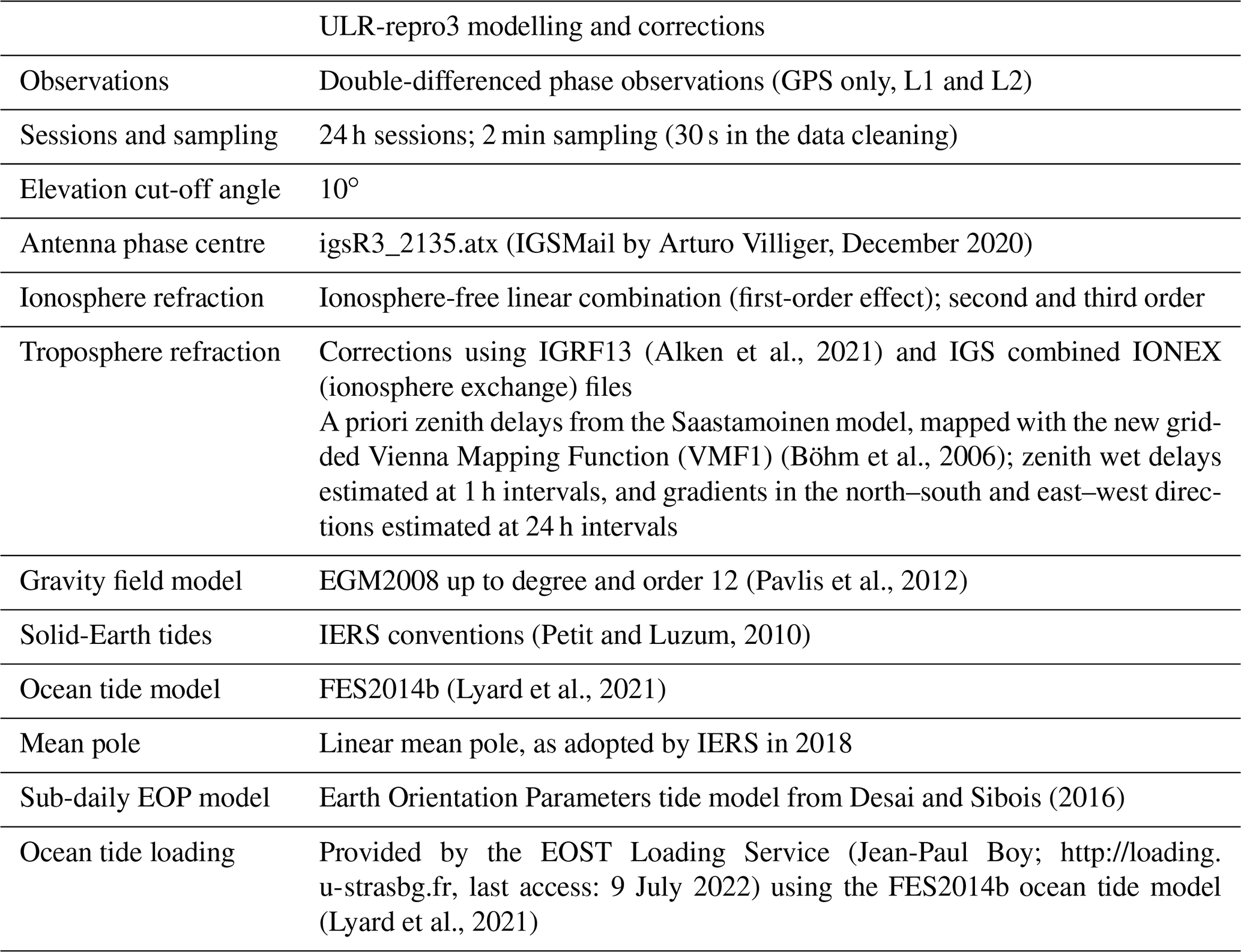
The remaining aspects of the ULR-repro3 data analysis strategy align with the approach used in Santamaria-Gomez et al. (2017); thus, they are only briefly outlined in the following in order to understand the analyst choices for geophysical application and interpretation. For each network of stations, double-differenced GPS phase observations were processed in the ionosphere-free linear combination of measurements on L1 and L2 frequencies. To minimise the impact of mismodelled low-elevation tropospheric delays, satellite observations below 10∘ were not considered. This cut-off angle aims to mitigate the limitation due to ground antennas without absolute calibration (13 % of the antennas in the ULR-repro3 network). These antennas have a relative calibration (with respect to an antenna with absolute calibration) converted to absolute considering only elevation-dependent phase centre variation (PCV) down to 10∘. For the other (calibrated) GNSS antennas, phase centre offsets with azimuth-dependent and elevation-dependent absolute PCV corrections were applied (igsR3_2135.atx; IGSMail by Arturo Villiger, 2020). Satellite-specific antenna phase centre offsets and block-specific nadir-angle-dependent absolute PCVs were applied for the transmitting antennas.
The first-order ionospheric delays were removed using the ionosphere-free linear combination observations, whereas the second and third orders were corrected using the International Geomagnetic Reference Field model (Alken et al., 2021) and total electron content maps from the IGS IONEX (ionosphere exchange) files. For the tropospheric delays, a priori hydrostatic zenith delays at the ellipsoidal surface were obtained for each station from the new gridded Vienna Mapping Function (VMF1) grids (Böhm et al., 2006). They were then reduced to the station heights using the GPT2 model (Lagler et al., 2013). The residual zenith tropospheric delays were adjusted at 1 h intervals (i.e. 25 parameters per day) for every station using a piecewise linear model, assuming that the unmodelled wet component dominates. Both the hydrostatic and wet zenith tropospheric delays were mapped to the observation elevations using the VMF1 functions. The azimuthal asymmetry in the tropospheric delay was accounted for by estimating a linear change in gradients (north–south and east–west) over each day and station using the mapping function from Chen and Herring (1997).
The phase observations were weighted by elevation angle in the first iteration and then by elevation angle and station-dependent scatter of the phase residuals obtained from the first iteration. The double-differenced phase ambiguities were adjusted to real values except when they could be confidently fixed to integer values (more than 85 % fixed). Within the same inversion, GNSS satellite orbital parameters were adjusted using 24 h arcs, IGS orbits as a priori values, and loose constraints consistent with the station position constraints (free-network approach). Non-gravitational constant and once-per-revolution accelerations on the satellites were adjusted too, using the ECOMC (Empirical CODE Orbit Model, where CODE stands for the Center for Orbit Determination in Europe) model. This model is a combination of the ECOM1 and ECOM2 models (Springer et al., 1999; Arnold et al., 2015) with specific parameters constrained in post-processing. Nominal satellite attitude corrections were applied, except during eclipse periods where yaw rates were modelled (Kouba, 2009). Phase rotations due to changes in the satellite antenna orientation away from the Earth-pointing direction were also applied (Wu et al., 1993). Regarding the Earth orientation parameters (pole position, rate, and length of day), these were estimated daily with a priori values from the IERS Bulletin A. Modelled diurnal and semi-diurnal terms were added to the a priori pole and UT1 values following the IERS Conventions (Petit and Luzum, 2010).
Note that neither loading displacements due to atmospheric tides nor non-tidal (atmospheric, oceanic, hydrologic) loading displacements were corrected during the first step, which aimed at estimating daily station positions from the GNSS measurements. By contrast, the displacements of the crust due to solid-Earth and pole tides (solid Earth and ocean) were corrected following the IERS Conventions (Petit and Luzum, 2010). Crustal motion due to the ocean tide loading was corrected too, using the tidal constituents computed by the EOST Loading Service at each station from the FES2014b model (Lyard et al., 2021).
2.2.2 Offset detection and terrestrial frame alignment
Figure 2 shows the number of stations selected for ULR-repro3 with GNSS observations available each day over the time period considered (2000.0–2021.0, in decimal years), ranging from 110+ to nearly 500 stations. For computational efficiency, the stations were split into several (up to 10) regional subnetworks, each having between 29 and 70 stations processed independently. For the reader interested in this technicality, Fig. S1 shows the regional subnetworks distribution for the day of 1 January 2018. An additional subnetwork of globally distributed stations was considered to allow the daily combination of the regional subnetwork results in a unique daily global solution. This global subnetwork was made up of IGS reference frame stations, each of which also appeared in one – and only one – of the regional subnetworks. In turn, one regional subnetwork included one IGS reference frame station at least but could include more depending on the total number of subnetworks. Moreover, to strengthen the physical link between regional subnetworks, two stations from adjacent regional subnetworks were also included, i.e. one station from one nearby subnetwork and another from another nearby subnetwork, exclusive of the stations in the global subnetwork. All the subnetworks vary day by day depending on the station data actually available for the day considered. This network strategy has changed compared with past ULR reanalyses, benefitting from the experience of the Massachusetts Institute of Technology (MIT) IGS analysis centre.

Figure 2(a) The evolution of station availability in ULR-repro3 (black) within a 15 or 1 km distance of a tide gauge (red and orange respectively) and within 15 km of a GLOSS tide gauge site (blue). (b) Spatial distribution of GNSS stations and their distance from the tide gauges considered in this study.
The loosely constrained station positions and tropospheric delays for the common stations and the satellite orbital and Earth rotation parameters estimated from the subnetwork data analyses were combined using GLOBK (Herring et al., 2015) to obtain the daily global solutions, which include all stations available each day with their positions expressed in a common but yet undetermined terrestrial frame. These daily global solutions were then stacked into a long-term solution using the CATREF software package (Altamimi et al., 2018) with a time-dependent functional model that included translation, rotation, and scale transformation parameters between daily and long-term frames, estimated simultaneously with the mean station positions (at the reference epoch 2010.5), annual and biannual signals, and velocities. The scale parameters, which represent the mean height changes of all the sites, are available upon request, especially for users interested in global sea level rise.
Note that position offset discontinuities (mostly due to equipment changes and earthquakes) as well as station velocity changes and post-seismic displacements (PSDs) were added to the above modelling, where appropriate. As experienced analysts still tend to perform better than automatic methods (Gazeaux et al., 2013), the position offsets were identified and adopted via expert visual assessment using all positioning components (i.e. including the north and east components). To facilitate this task, the equipment changes reported in the GNSS station logs were considered along with the co-seismic displacements larger than 2 mm predicted with the earthquakes database and modelling by Métivier et al. (2014). When a position discontinuity was detected in a time series, the station position was estimated separately before and after the discontinuity along with the offset amplitude. The velocities before and after each position discontinuity were tightly constrained (0.01 mm yr−1), unless a velocity discontinuity was suspected. In the latter case (less than 2 % of the GNSS stations considered in ULR-repro3), no constraint was applied, and different velocities were estimated for each period of data around the discontinuity.
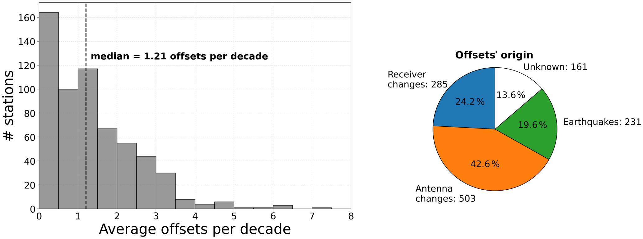
Figure 3Average station position offsets per decade (histogram) and offsets' origins (pie chart).
The above procedure also included manual editing to identify (and remove) outliers as well as additional non-documented position offset discontinuities. It was iterated until convergence (expert visual assessment). Overall, 1.2 offset discontinuities were detected per decade and per station, mostly caused by equipment changes (66.8 %) and earthquakes (19.6 %), whereas the remaining 13.6 % were flagged as unknown (Fig. 3) due to the lack of available metadata.
The long-term terrestrial frame, in which the estimated velocities are ultimately expressed, was finally aligned to the ITRF2014 (Altamimi et al., 2017) by applying minimal constraints to all the transformation parameters (translation, rotation, scale, and their rates) with respect to the positions and velocities of a stable subset of about 35 well-distributed reference frame stations. This step resulted in daily position time series expressed in the ITRF2014 frame for all (601) stations considered in ULR-repro3. From this set of position time series, only stations with more than 3 years between two consecutive position discontinuities and with data gaps not exceeding 30 % were retained for the next step as input (546 stations, among which 161 are reference stations and 457 are near a tide gauge).
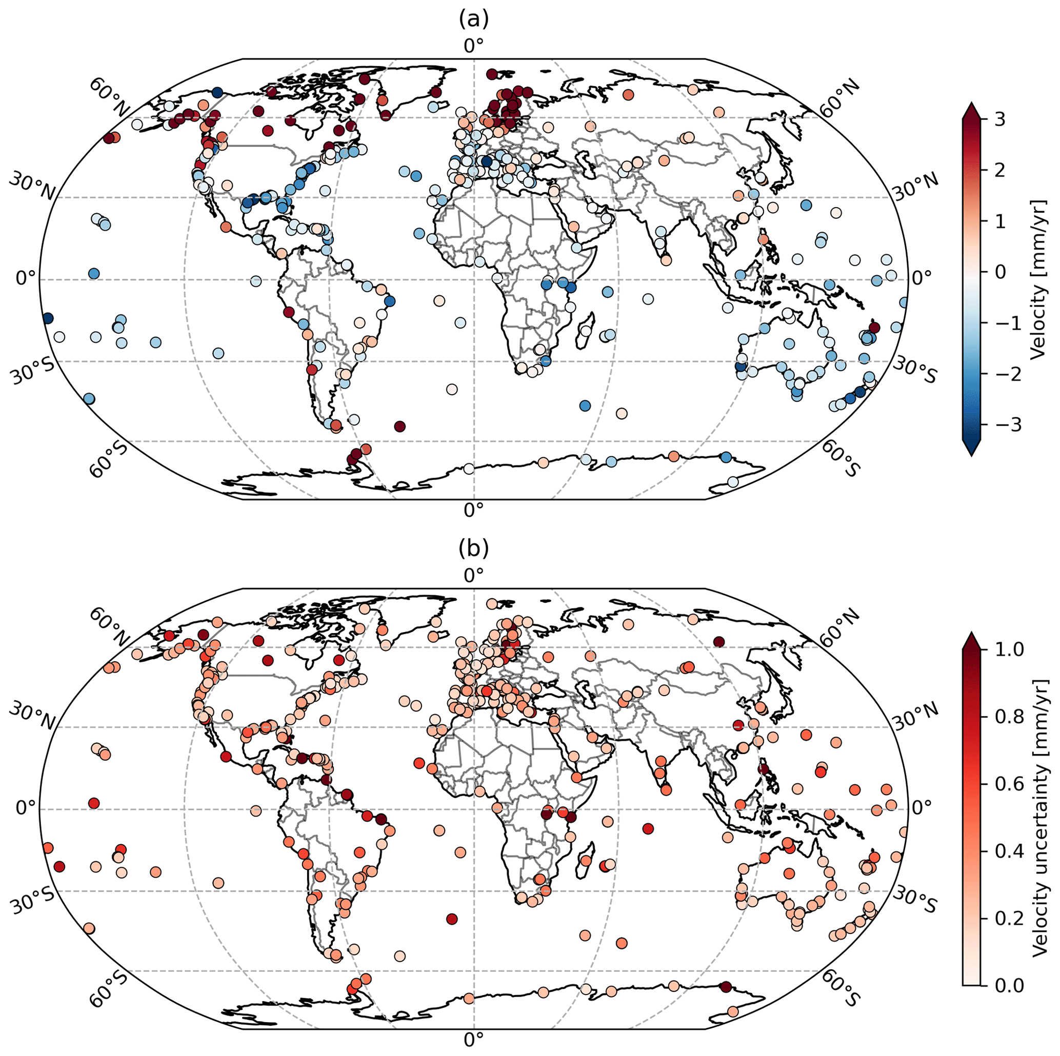
Figure 4Vertical velocities (a) and associated uncertainties (b) estimated for the stations with at least 3 years of continuous measurement (see text).
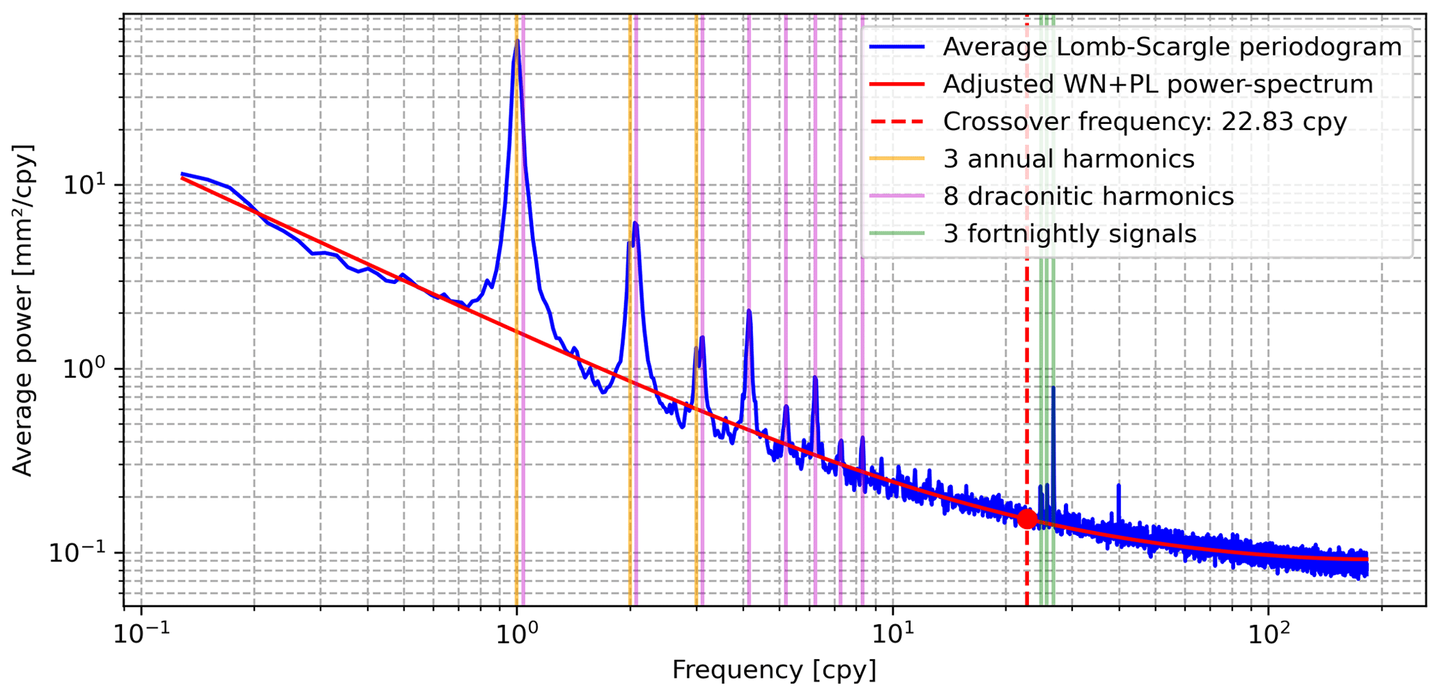
Figure 5Average Lomb–Scargle periodogram for the ULR-repro3 detrended vertical position time series corrected for NTAL displacements (frequency unit is cycles per year, denoted as “cpy”).
2.2.3 Stochastic modelling and time-correlated noise
The last step was the estimation of the parameters of interest (primarily station velocities) and their uncertainties, where both a functional and a stochastic model were adjusted to each of the position time series found using the procedure described in Sect. 2.2.1 on a station-by-station basis, as follows:
where xref is the position at the reference epoch tref, defined arbitrarily as the mid of the observation period considered (2000.0–2021.0); vx is the linear velocity; is the Heaviside function that multiplies the position offset ai; is the period (in years) of the seasonal term j (annual, biannual and triannual); is the period (in years) (PD in days) of the draconitic signals; and is the period (in years) (PF in days) of the fortnightly signals.
In this step, an additional and independent time series editing was considered to eliminate any possible remaining unreliable estimates from the previous step. The position estimates were compared to a running monthly median. Any epoch with a position showing a difference from the median exceeding 5 times the median absolute deviation in at least one component was discarded.
The stochastic model considered a linear combination of white noise (WN) and the power-law (PL) process (WN + PL), whose parameters (the stochastic process amplitudes and the spectral index of the power-law process) were estimated using the restricted maximum likelihood estimation method (Patterson and Thompson, 1971; Koch, 1986; Gobron et al., 2022). To obtain realistic stochastic parameter estimates, non-tidal atmospheric loading (NTAL) displacements were also subtracted from the position time series prior to this adjustment, following the recommendation of Gobron et al. (2021). These NTAL displacements were obtained from the Earth System Modelling team of the German Research Centre for Geosciences in Potsdam (Dill and Dobslaw, 2013).
The functional model included an intercept, a linear trend (velocity), the position offsets identified in the previous step, three seasonal terms (annual, biannual, and triannual), periodic terms at the first eight harmonics of the GPS draconitic year (351.4 d; Ray et al., 2008), and three fortnightly terms with respective periods of 13.62, 14.19, and 14.76 d (Penna and Stewart, 2003; Amiri-Simkooei, 2013). The parameters of this functional model and their uncertainties were estimated using the weighted least squares estimator with the inverse of the estimated WN + PL model covariance matrix as the weight matrix. During the observation time span, some stations (44) recorded significant co-seismic offsets and transient post-seismic signals, in which case the modelling was further extended to include velocity changes, and logarithmic or exponential decay functions according to the observed time evolution.
2.3 Estimates of vertical land motion
The GNSS products of primary interest for sea level studies are the station position time series and vertical velocity estimates, as underlined in the founding charter of the IGS working group “GNSS Tide Gauge Benchmark Monitoring” (Schöne et al., 2009) and later on in the implementation plan of the GLOSS programme (IOC, 2012). In the following, we focus on the vertical positioning component; however, the horizontal components are made available too and can be useful for other geophysical applications. Figure 4 shows the ULR-repro3 vertical velocity field and the corresponding uncertainties. This GNSS velocity field ultimately consists of 546 stations, among which 457 are within 15 km of a tide gauge. This number decreases to 135 for stations less than 1 km from a tide gauge. Note that the stations inland are IGS reference frame stations (Sect. 2.1).
Overall, the geographical patterns observed in Fig. 4a are consistent with known geophysical processes, such as uplift in the northern latitudes of Europe and North America due to glacial isostatic adjustment (GIA) or subsidence along the northern coastlines of the Gulf of Mexico primarily driven by groundwater depletion and sediment compaction, also observed in previous and independent GNSS analysis results (e.g. Blewitt et al., 2018; Hammond et al., 2021). The eight stations with velocity discontinuities are not plotted in Fig. 4.
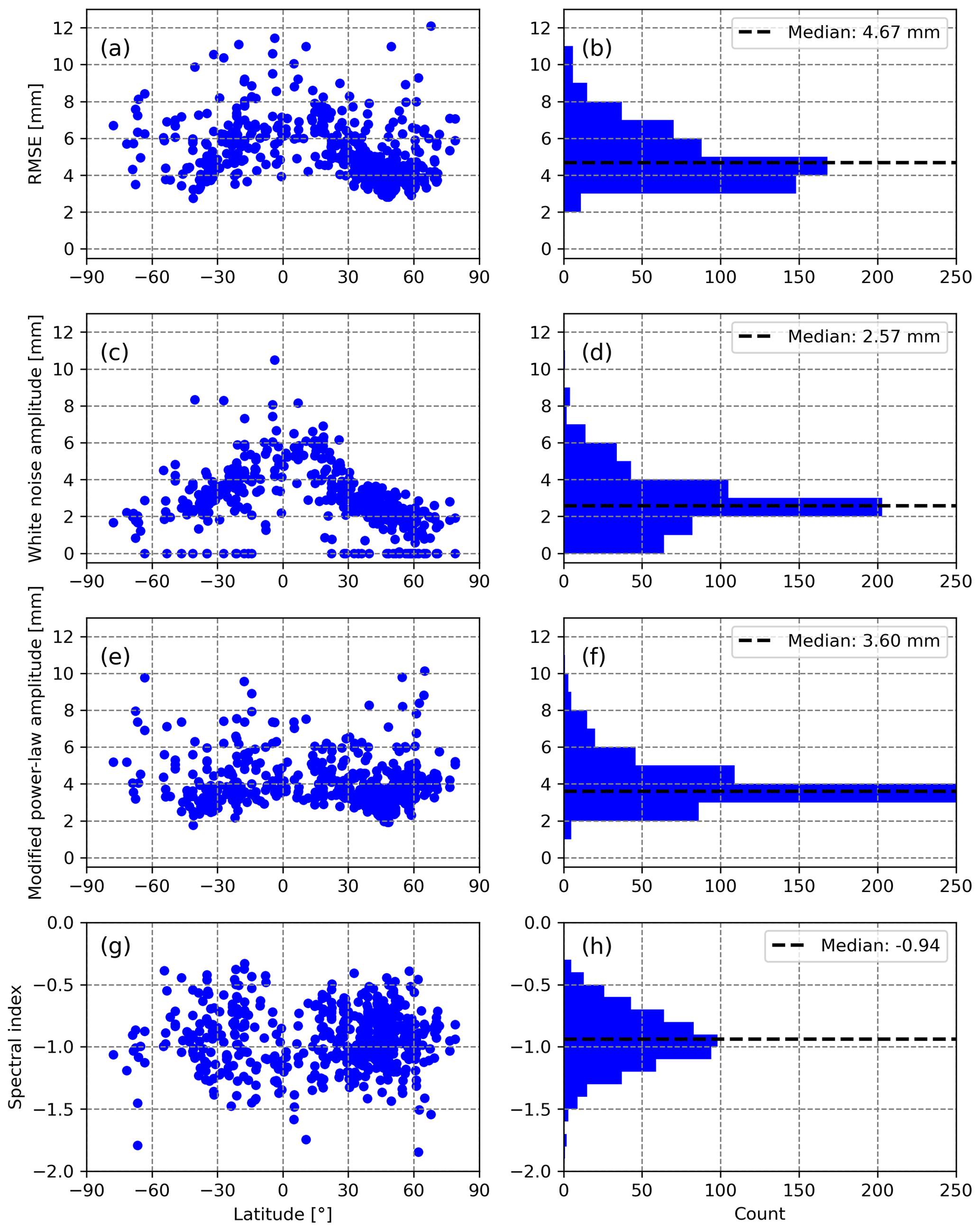
Figure 6Vertical position time series of (a, b) RMSE values, (c, d) white noise amplitudes, (e, f) modified power-law amplitudes, and (g, h) spectral indices. See the text for details.
3.1 Average time correlation properties
Previous studies have documented the presence of both power-law noise and white noise in GNSS station position time series (e.g. Williams et al., 2004; Santamaria-Gomez et al., 2011; Gobron et al., 2021; Santamaria-Gomez and Ray, 2021). Such time-correlated properties are also evidenced by Fig. 5 for ULR-repro3, where Lomb–Scargle periodograms of all detrended station position time series were averaged. As highlighted by the red curve in Fig. 5 (on logarithmic scales), the power-law process induces a negative trend at low frequencies (i.e. a spectral power ), whereas white noise causes a flattening at high frequencies. This flattening is especially visible above 22.8 cpy (cycles per year), where the power of the white noise exceeds that of the power-law process. Note that, on the one hand, the background shape of the average periodogram (Fig. 5) is accounted for by the WN + PL stochastic model, presented in Sect. 2.2.3, and adjusted to each position time series. On the other hand, the functional model accounts for the spectral peaks marked by coloured vertical lines, which correspond to well-identified periodic oscillations common to most GPS solutions (Ray et al., 2008).
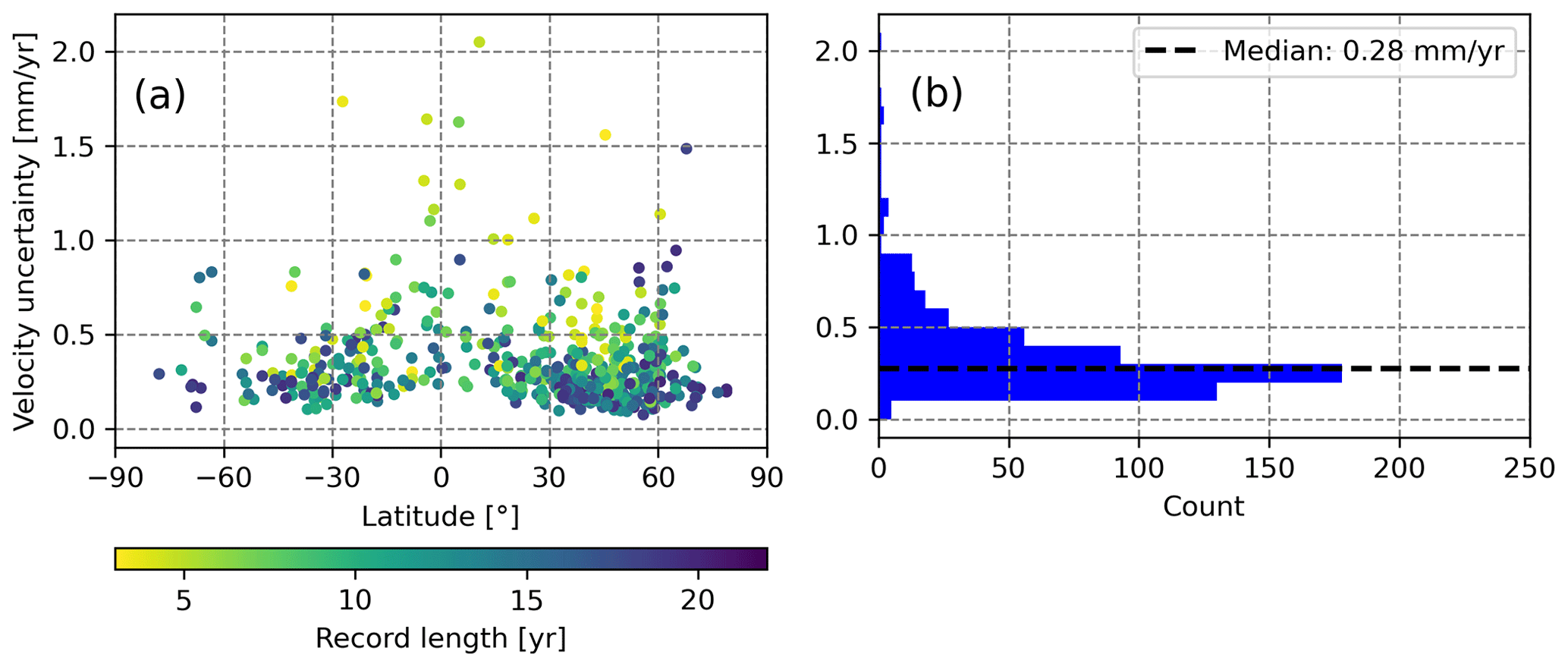
Figure 7Vertical velocity uncertainties (a) as a function of the geographical latitude with the colour corresponding to the record length and (b) histogram.
3.2 Stochastic properties of position time series
The periodogram in Fig. 5 does not provide information about the properties of individual stations. By contrast, Fig. 6 highlights the stochastic process amplitudes and the spectral index of the WN + PL stochastic models adjusted to the individual vertical position time series.
The median value of the spectral indices is −0.94, i.e. close to −1.00, which confirms the prevalence of a flicker-like noise in the low-frequency band. The spectral indices show no clear latitudinal dependency (Fig. 6g, h). As power-law amplitudes depend on the spectral index values, they were transformed into a modified empirical standard deviation (Gobron et al., 2021), expressed in millimetres, enabling a more rigorous comparison between noise amplitudes and root mean squared error (RMSE) values. No latitudinal dependency is revealed in Fig. 6e. By contrast, the white noise amplitudes show the largest values within the tropical band (Fig. 6c) and lower values at high latitude, but they are mostly non-zero thanks to the NTAL corrections (Gobron et al., 2021). Logically, this pattern also appears in the RMSE (Fig. 6a), as it quantifies the combined influence of the white noise and power-law processes.
3.3 Vertical velocity uncertainties
An important consequence of temporally correlated noise in time series of GNSS positions is its impact on the uncertainties in GNSS-derived velocities, which can be largely underestimated, up to a factor of 10 (Williams et al., 2004), if the temporal correlations are ignored. Figure 7 shows the distribution of the vertical velocity uncertainties obtained for the ULR-repro3 stations considering the stochastic properties estimated above. Their median value is 0.27 mm yr−1, with 83 % of the stations displaying a vertical velocity uncertainty below 0.5 mm yr−1. The colouring in Fig. 7a indicates that the largest velocity uncertainties typically correspond to the stations with the shortest records.
3.4 Highlights with respect to the previous ULR reanalysis
To appraise the progress accomplished with the ULR-repro3 reanalysis, the position time series from the previous reanalysis (Santamaria-Gomez et al., 2017) were retrieved at SONEL, and the same processing (last step in Sect. 2) was applied for a rigorous comparison (the same non-tidal atmospheric loading corrections and the same functional and stochastic models). This comparison involved the 251 common stations. Figure 8 indicates a substantial reduction of 28 % in the median vertical velocity uncertainties, from 0.35 mm yr−1 down to 0.25 mm yr−1 (ULR-repro3), which is below the uncertainty threshold reported by Griffiths and Ray (2016) using simulations to investigate the effect of position offsets and record lengthening. However, it is worth noting that the community interested in monitoring vertical land motion at tide gauges tends to limit changes in GNSS equipment to the strictly unavoidable (failure, destruction, etc.), as recommended by the IGS-related working group (Schöne et al., 2009). As a result, the average return period of offsets is about 4 years longer here (Fig. 3) than observed for the entire set of stations contributing to the third IGS reanalysis campaign (Rebischung et al., 2021), thereby partly explaining the improved velocity uncertainties observed with ULR-repro3 reanalysis.
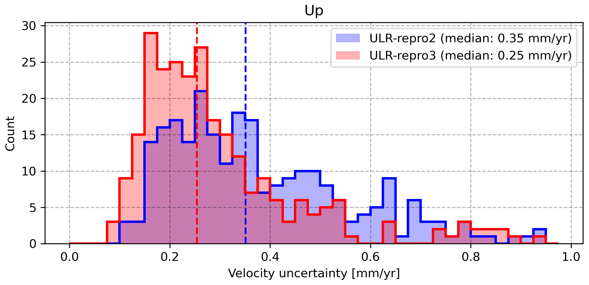
Figure 8Vertical velocity uncertainties for ULR-repro3 with respect to the previous ULR solution based on the 251 common stations. The vertical dashed lines correspond to the medians.
The marked improvement in the quality of ULR-repro3 products can also be appraised from the RMSE position residuals (median value of 5.3 mm reduced to 4.9 mm) and the amplitude of white noise (from 3.4 to 2.8 mm), whereas the power-law amplitude and spectral index remained equivalent (3.8 mm and −0.93 respectively).
In addition to the progress achieved over the previous ULR solution, the quality of the ULR-repro3 solution was also confirmed by the comparisons undertaken within the IGS reanalysis campaign, showing that the noise content in ULR-repro3 is comparable to that of most of the other contributing solutions and analysis centres (Rebischung et al., 2021).
The ULR-repro3 products are available from the online digital object identifier (DOI) landing page (https://doi.org/10.26166/sonel_ulr7a; Gravelle et al., 2022) and comprise the station position time series and the estimated velocities for all positioning components (north, east, and up). These products are hosted at the SONEL scientific service, which serves as a data assembly centre dedicated to GNSS data at tide gauges (Wöppelmann et al., 2021) for the international GLOSS programme (IOC, 2012). As a UNESCO-related programme, the service complies with the UNESCO open-access data policy (i.e. the data sets are available free of charge without any barriers) and strives towards providing the highest international standards, in particular in terms of long-term availability and permanent access. Note that the ULR-repro3 reanalysis yielded other parameter estimates that could be of interest for other geophysical applications (e.g. station position offsets related to earthquakes and seasonal signals). These are also made available via SONEL.
This paper has presented the latest GNSS data reanalysis carried out by the ULR group within the international IGS framework, yielding time series of position estimates to measure the vertical land motion near tide gauges. It includes an increased number of GNSS stations with an extended time span. Along with the velocity estimates, their uncertainties were obtained by modelling the temporally correlated noise processes inherent in the data, after correcting the position time series for non-tidal atmospheric loading displacements, as recommended by Gobron et al. (2021). Overall, the comparisons indicate that ULR-repro3 represents a marked improvement in product quality over the previous reanalysis, with a notable 28 % reduction in median vertical velocity uncertainty (Fig. 8).
An interesting perspective will be to examine the differences with global reanalyses obtained by other groups complying with the latest IGS standards but using different analyst choices at any of the major GNSS processing steps described in Sect. 2 (e.g. Blewitt et al., 2016; Männel et al., 2022). A related perspective will be to address the issue of which reanalysis is best for the non-expert sea level user, if any (Ballu et al., 2019). In this respect, the Commission on Mean Sea Level and Tides from the International Association for the Physical Sciences of the Oceans (IAPSO) could provide a stimulating framework to gather experts and users worldwide and to reflect on the issue posed by multiple high-quality GNSS reanalyses, as IAPSO did nearly 30 years ago when the issue of geodetic fixing of tide gauge benchmarks was considered with the advances of space geodesy (Carter et al., 1994).
The supplement related to this article is available online at: https://doi.org/10.5194/essd-15-497-2023-supplement.
The project was defined by MGr and GW as a contribution to the third reprocessing (“repro3”) campaign of the International GNSS Service (IGS). MGr processed the GPS data with support from TH (GAMIT/GLOBK software packages, network design, and strategy for subnetwork design and orbit adjustment), ZA (CATREF software and reference frame alignment), PR (product quality assessment within “repro3”), and MGu (strategic use of the high-performance computing centre). KG prepared the NTAL corrections, assessed the stochastic properties of the time series, and produced the final velocity field. All authors contributed to the analysis and discussion of the results. The first manuscript draft was written by GW. All authors contributed to the subsequent versions and approved the final manuscript.
The contact author has declared that none of the authors has any competing interests.
Publisher's note: Copernicus Publications remains neutral with regard to jurisdictional claims in published maps and institutional affiliations.
Our study benefited tremendously from agencies making their data available to IGS and SONEL. The authors would like to acknowledge the crucial role played by the high-performance computing centre of La Rochelle University, especially the Mozart and Thor supercomputers. We are grateful to Laurent Métivier for providing the modelled earthquake displacements and to Jean-Paul Boy for the ocean tidal loading corrections. Finally, we would like to thank both anonymous reviewers for their comments that contributed to improving the paper.
This research has been supported by the CNRS/INSU research agency via the SONEL and RENAG observation systems. In addition, part of this research was made possible by support from NASA (grant no. 80NSSC18K0457) and the NSF (grant no. NSF-IF-1843686).
This paper was edited by Alessio Rovere and reviewed by two anonymous referees.
Alken, P., Thébault, E., Beggan, C. D., Amit, H., Aubert, J., Baerenzung, J., Bondar, T. N., Brown, W. J., Califf, S., Chambodut, A., Chulliat, A., Cox, G. A., Finlay, C. C., Fournier, A., Gillet, N., Grayver, A., Hammer, M. D., Holschneider, M., Huder, L., Hulot, G., Jager, T., Kloss, C., Korte, M., Kuang, W., Kuvshinov, A., Langlais, B., Léger, J.-M., Lesur, V., Livermore, P. W., Lowes, F. J., Macmillan, S., Magnes, W., Mandea, M., Marsal, S., Matzka, J., Metman, M. C., Minami, T., Morschhauser, A., Mound, J. E., Nair, M., Nakano, S., Olsen, N., Pavón-Carrasco, F. J., Petrov, V. G., Ropp, G., Rother, M., Sabaka, T. J., Sanchez, S., Saturnino, D., Schnepf, N. R., Shen, X., Stolle, C., Tangborn, A., Tøffner-Clausen, L., Toh, H., Torta, J. M., Varner, J., Vervelidou, F., Vigneron, P., Wardinski, I., Wicht, J., Woods, A., Yang, Y., Zeren, Z., and Zhou, B.: International Geomagnetic Reference Field: the thirteenth generation, Earth Planets Space, 73, 49, https://doi.org/10.1186/s40623-020-01288-x, 2021.
Altamimi, Z., Boucher, C., and Sillard, P.: New trends for the realization of the International Terrestrial Reference System, Adv. Space Res., 30, 175–184, 2002.
Altamimi, Z., Métivier, L., Rebischung, P., Rouby, H., and Collilieux, X.: ITRF2014 plate motion model, Geophys. J. Int., 209, 1906–1912, 2017.
Altamimi, Z., Boucher, C., Sillard, P., Collilieux, X., and Rebischung, P.: CATREF software (Combination and Analysis of Terrestrial Reference Frames), Manual, version of 19 April 2018.
Amiri-Simkooei, A. R.: On the nature of GPS draconitic year periodic pattern in multivariate position time series, J. Geophys. Res.-Sol. Ea., 118, 2500–2511, https://doi.org/10.1002/jgrb.50199, 2013.
Arnold, D., Meindl, M., Beutler, G., Dach, R., Schaer, S., Lutz, S., Prange, L., Sośnica, K., Mervart, L., and Jäggi, A.: CODE's new solar radiation pressure model for GNSS orbit determination, J. Geod., 89, 775–791, 2015.
Ballu, V., Gravelle, M., Wöppelmann, G., de Viron, O., Rebischung, P., Becker, M., and Sakic, P.: Vertical land motion in the Southwest and Central Pacific from available GNSS solutions and implications for relative sea levels, Geophys. J. Int., 218, 1537–1551, https://doi.org/10.1093/gji/ggz247, 2019.
Blewitt, G., Kreemer, C. Hammond, W. C., and Gazeaux, J.: MIDAS robust trend estimator for accurate GPS station velocities without step detection, J. Geophys. Res.-Sol. Ea., 121, 2054–2068, https://doi.org/10.1002/2015JB012552, 2016.
Blewitt, G., Hammond, W. C., and Kreemer, C.: Harnessing the GPS data explosion for interdisciplinary science, Eos, 99, 1–2, https://doi.org/10.1029/2018EO104623, 2018.
Böhm, J., Werl, B., and Schuh, H.: Troposphere mapping functions for GPS and very long baseline interferometry from European Centre for Medium-Range Weather Forecasts operational analysis data, J. Geophys. Res., 111, B02406, https://doi.org/10.1029/2005JB003629, 2006.
Carter, W. E. (Ed.): Report of the surrey workshop of the IAPSO tide gauge benchmark fixing committee, Report of a meeting held 13–15 December 1993 at the Inst. of Oceanog. Sci., Deacon Lab., NOAA Tech. Rep., NOSOES0006, 1994.
Chen, G. and Herring, T. A.: Effects of atmospheric azimuthal asymmetry on the analysis of space geodetic data, J. Geophys. Res., 102, 20489–20502, 1997.
Desai, S. D. and Sibois, A. E.: Evaluating predicted diurnal and semidiurnal tidal variations in polar motion with GPS-based observations, J. Geophys. Res.-Sol. Ea., 121, 5237–5256, https://doi.org/10.1002/2016JB013125, 2016.
Dill, R. and Dobslaw, H.: Numerical simulations of global-scale high-resolution hydrological crustal deformations, J. Geophys. Res.-Sol. Ea., 118, 5008–5017, https://doi.org/10.1002/jgrb.50353, 2013.
Frederikse, T., Landerer, F., Caron, L., Adhikari, S., Parkes, D., Humphrey, V. W., Dangendorf, S., Hogarth, P., Zanna, L., Cheng, L., and Wu, Y.-H.: The causes of sea-level rise since 1900, Nature, 584, 393–397, https://doi.org/10.1038/s41586-020-2591-3, 2020.
Gazeaux, J., Williams, S., King, M., Bos, M., Dach, R., Deo, M., Moore, A. W., Ostini, L., Petrie, E., Roggero, M., Teferle, F. N., Olivares, G., and Webb, F. H.: Detecting offsets in GPS time series: First results from the detection of offsets in GPS experiment, J. Geophys. Res.-Sol. Ea., 118, 2397–2407, https://doi.org/10.1002/jgrb.50152, 2013.
Gobron, K., Rebischung, P., Van Camp, M., Demoulin, A., and de Viron, O.: Influence of aperiodic non-tidal atmospheric and oceanic loading deformations on the stochastic properties of global GNSS vertical land motion time series, J. Geophys. Res.-Sol. Ea., 126, e2021JB022370, https://doi.org/10.1029/2021JB022370, 2021.
Gobron, K., Rebischung, P., de Viron, O., Demoulin, A., and Van Camp, M.: Impact of offsets on assessing the low-frequency stochastic properties of geodetic time series, J. Geod., 96, 42, https://doi.org/10.1007/s00190-022-01634-9, 2022.
Gravelle, M., Wöppelmann, G. M., Gobron, K., Altamimi, Z., Guichard, M., Herring, T., and Rebischung, P.: The ULR-repro3 GPS data reanalysis solution (aka ULR7a), SONEL Data Center [data set], https://doi.org/10.26166/sonel_ulr7a, 2022.
Griffiths, J. and Ray, J.: Impacts of GNSS position offsets on global frame stability, Geophys. J. Int., 204, 480–487, https://doi.org/10.1093/gji/ggv455, 2016.
Hamlington, B. D., Gardner, A. S., Ivins, E., Lenaerts, J. T. M., Reager, J. T., Trossman, D. S., Zaron, E. D., Adhikari, S., Arendt, A., Aschwanden, A., Beckley, B. D., Bekaert, D. P. S., Blewitt, G., Caron, L., Chambers, D. P., Chandanpurkar, H. A., Christianson, K., Csatho, B., Cullather, R. I., DeConto, R. M., Fasullo, J. T., Frederikse, T., Freymueller, J. T., Gilford, D. M., Girotto, M., Hammond, W. C., Hock, R., Holschuh, N., Kopp, R. E., Landerer, F., Larour, E., Menemenlis, D., Merrifield, M., Mitrovica, J. X., Nerem, R. S., Nias, I. J., Nieves, V., Nowicki, S., Pangaluru, K., Piecuch, C. G., Ray, R. D., Rounce, D. R., Schlegel, N.-J., Seroussi, H., Shirzaei, M., Sweet, W. V., Velicogna, I., Vinogradova, N., Wahl, T., Wiese, D. N., and Willis, M. J.: Understanding of contemporary regional sea-level change and the implications for the future, Rev. Geophys., 58, e2019RG0000672, https://doi.org/10.1029/2019RG000672, 2020.
Hammond, W. C., Blewitt, G., Kreemer, C., and Nerem, R. S.: GPS imaging of global vertical land motion for studies of sea level rise, J. Geophys. Res.-Sol. Ea., 126, e2021JB022355, https://doi.org/10.1029/2021JB022355, 2021.
Heflin, M., Bertiger, W., Blewitt, G., Freedman, A., Hurst, K., Lichten, S., Lindqwister, U., Vigue, Y., Webb, F., Yunck, T., and Zumberge, J.: Global geodesy using GPS without fiducial sites, Geophys. Res. Lett., 19, 131–134, 1992.
Herring, T. A., Floyd, M. A., and McClusky, S. C.: GLOBK Reference Manual, release 10.6, http://geoweb.mit.edu/gg/ (last access: 9 July 2022), 16 June 2015.
Herring, T. A., King, R. W., Floyd, M. A., King, R. W., and McClusky, S. C.: GAMIT Reference Manual, release 10.7, http://geoweb.mit.edu/gg/ (last access: 9 July 2022), 7 June 2018.
IOC: Global Sea-Level Observing System (GLOSS) Implementation Plan (2012), IOC Tech. Ser., Vol. 100, 41 pp., 2012.
Johnston, G., Riddell, A., and Hausler, G.: The International GNSS Service, Springer Handbook of Global Navigation Satellite Systems, 967–982, https://doi.org/10.1007/978-3-319-42928-1_33, 2017.
Koch, K: Maximum likelihood estimate of variance components, Bulletin Géodésique, 60, 329–338, https://doi.org/10.1007/BF02522340, 1986.
Kouba, J.: A simplified yaw-attitude model for eclipsing GPS satellites, GPS Solut., 13, 1–12, https://doi.org/10.1007/s10291-008-0092-1, 2009.
Lagler, K., Schindelegger, M., Böhm, J., Krásná, H., and Nilsson, T.: GPT2: Empirical slant delay model for radio space geodetic techniques, Geophys. Res. Lett., 40, 1069–1073, https://doi.org/10.1002/grl.50288, 2013.
Lyard, F. H., Allain, D. J., Cancet, M., Carrère, L., and Picot, N.: FES2014 global ocean tide atlas: design and performance, Ocean Sci., 17, 615–649, https://doi.org/10.5194/os-17-615-2021, 2021.
Magnan, A. K., Schipper, E. L. F., and Duvat, V. K. E.: Frontiers in climate change adaptation science: advancing guidelines to design adaptation pathways, Curr. Clim. Change Rep., 6, 166–177, https://doi.org/10.1007/s40641-020-00166-8, 2020.
Männel, B., Schöne, T., Bradke, M., and Schuh, H.: Vertical land motion at tide gauges observed by GNSS: a new GFZ-TIGA solution, in: International Association of Geodesy Symposia, Springer, Berlin, Heidelberg, https://doi.org/10.1007/1345_2022_150, 2022.
Marcos, M., Wöppelmann, G., Matthews, A., Ponte, R. M., Birol, F., Ardhuin, F., Coco, G., Santamaria-Gomez, A., Ballu, V., Testut, L., Chambers, D., and Stopa, J. E.: Coastal sea level and related fields from existing observing systems, Surv. Geophys., 40, 1293–1317, https://doi.org/10.1007/s10712-019-09513-3, 2019.
Métivier, L., Collilieux, X., Lercier, D., Altamimi, Z., and Beauducel, F.: Global coseismic deformations, GNSS time series analysis, and earthquake scaling laws, J. Geophys. Res.-Sol. Ea., 119, 9095–9109, 2014.
Patterson, H. D. and Thompson, R.: Recovery of inter-block information when block sizes are unequal, Biometrika, 58, 545–554, https://doi.org/10.1093/biomet/58.3.545, 1971.
Pavlis, N. K., Holmes, S. A., Kenyon, S. C., and Factor, J. K.: The development and evaluation of the Earth Gravitational Model 2008 (EGM2008), J. Geophys. Res., 117, B04406, https://doi.org/10.1029/2011JB008916, 2012.
Penna, N. T. and Stewart, M. P.: Aliased tidal signatures in continuous GPS height time series, Geophys. Res. Lett., 30, 2184, https://doi.org/10.1029/2003GL018828, 2003.
Petit, G. and Luzum, B.: IERS conventions, Tech. Note 36, Bureau International des Poids et Mesures, Sevres (France), https://iers-conventions.obspm.fr/ (last access: 9 July 2022), 2010.
Poitevin, C., Wöppelmann, G., Raucoules, D., Le Cozannet, G., Marcos, M., and Testut, L.: Vertical land motion and relative sea level changes along the coastline of Brest (France) from combined space-borne geodetic methods, Remote Sens. Environ., 222, 275–285, https://doi.org/10.1016/j.rse.2018.12.035, 2019.
Ray, J., Altamimi, Z., Collilieux, X., and van Dam, T.: Anomalous harmonics in the spectra of GPS position estimates, GPS Solut., 12, 55–64, https://doi.org/10.1007/s10291-007-0067-7, 2008.
Rebischung, P.: Terrestrial frame solutions from the IGS third reprocessing, EGU General Assembly 2021, online, 19–30 April 2021, EGU21-2144, https://doi.org/10.5194/egusphere-egu21-2144, 2021.
Rebischung, P., Altamimi, Z., Ray, J., and Garayt, B.: The IGS contribution to ITRF2014, J. Geodesy, 90, 611–630, https://doi.org/10.1007/s00190-016-0897-6, 2016.
Rebischung, P., Collilieux, X., Métivier, L., Altamimi, Z., and Chanard, K.: Analysis of IGS repro3 Station Position Time Series, AGU Fall Meeting, 13–17 December 2021, https://doi.org/10.1002/essoar.10509008.1, 2021.
Sanli, D. U. and Blewitt, G.: Geocentric sea level trend using GPS and >100-year tide gauge record on a postglacial rebound nodal line, J. Geophys. Res., 106, 713–719, https://doi.org/10.1029/2000JB900348, 2001.
Santamaria-Gomez, A. and Ray, J.: Chameleonic noise in GPS position time series, J. Geophys. Res.-Sol. Ea., 126, e2020JB019541, https://doi.org/10.1029/2020JB019541, 2021.
Santamaria-Gomez, A., Bouin, M.-N., Collilieux, X., and Wöppelmann, G.: Correlated errors in GPS position time series: Implications for velocity estimates, J. Geophys. Res., 116, B01405, https://doi.org/10.1029/2010JB007701, 2011.
Santamaria-Gomez, A., Gravelle, M., Dangendorf, S., Marcos, M., Spada, G., and Wöppelmann, G.: Uncertainty of the 20th century sea-level rise due to vertical land motion errors, Earth Planet. Sc. Lett., 473, 24–32, 2017.
Schöne, T., Schön, N., and Thaller, D.: IGS Tide gauge benchmark monitoring pilot project (TIGA): scientific benefits, J. Geod., 83, 249–261, https://doi.org/10.1007/s00190-008-0269-y, 2009.
Springer, T. A., Beutler, G., and Rothacher, M.: A new solar radiation pressure model for GPS, Adv. Space Res., 23, 673–676, https://doi.org/10.1016/S0273-1177(99)00158-1, 1999.
Steigenberger, P., Rothacher, M., Dietrich, R., Fritsche, M., Rülke, A., and Vey, S.: Reprocessing of a global GPS network, J. Geophys. Res., 111, B05402, https://doi.org/10.1029/2005JB003747, 2006.
Williams, S. D. P., Bock, Y., Fang, P., Jamason, P., Nikolaidis, R. M., Prawirodirdjo, L., Miller, M., and Johnson, D. J.: Error analysis of continuousGPS position time series, J. Geophys. Res., 109, B03412, https://doi.org/10.1029/2003JB002741, 2004.
Woodworth, P. L., Melet, A., Marcos, M., Ray, R. D., Wöppelmann, G., Sasaki, Y. N., Cirano, M., Hibbert, A., Huthnance, J. M., Monserrat, S., and Merrifield, M. A.: Forcing factors affecting sea level changes at the coast, Surv. Geophys., 40, 1351–1397, 2019.
Wöppelmann, G. and Marcos, M.: Vertical land motion as a key to understanding sea level change and variability, Rev. Geophys., 54, 64–92, 2016.
Wöppelmann, G., Martin Miguez, B., Bouin, M.-N., and Altamimi, Z.: Geocentric sea-level trend estimates from GPS analyses at relevant tide gauges world-wide, Global Planet. Change, 57, 396–406, https://doi.org/10.1016/j.gloplacha.2007.02.002, 2007.
Wöppelmann, G., Letetrel, C., Santamaria, A., Bouin, M.-N., Collilieux, X., Altamimi, Z., Williams, S. D. P., and Martin Miguez, B.: Rate of sea-level change over the past century in a geocentric reference frame, Geophys. Res. Lett., 36, L12607, https://doi.org/10.1029/2009GL038720, 2009.
Wöppelmann, G., Gravelle, M., and Testut, L.: SONEL sea-level observing infrastructure: French contribution to the IUGG Centennial in 2019 and beyond, Collection du Bureau des Longitudes, 1, 43–53, ISBN 978-2-491688-08-0, 2021.
Wu, J. T., Wu, S. C., Hajj, G. A., Bertiger, W. I., and Lichten, S. M.: Effects of antenna orientation on GPS carrier phase, Manuscr. Geodaet. 18, 91–98, 1993.