Last Glacial loess in Europe: luminescence database and chronology of deposition

During the Last Glacial Period, the climate shift to cold conditions associated with changes in atmospheric circulation and vegetation cover resulted in the development of large aeolian systems in Europe. On a regional scale, many factors may have influenced dust dynamics, such as the latitudinal difference between the various aeolian systems and the variability of the sources of wind-transported particles. Therefore, the assumption that the timing of aeolian deposition is strictly synchronous in Europe does not seem to be the most plausible hypothesis and needs to be evaluated. To test this assumption, the chronology of loess deposition in different European regions was investigated by studying 93 luminescence-dated loess–palaeosol sequences with their data recalculated and compiled in a single comma separated values (*.csv) file: the ChronoLoess database. Our study shows that the two major aeolian systems, the Northern European Loess Belt (NELB) on the one hand and the systems associated with the rivers draining the Alpine Ice Sheet on the other hand, developed asynchronously. The significant deposition started at about 32 kyr b2k for the NELB vs. 42 kyr b2k for the perialpine loess and peaked about 2 millennia later for the former (21.8 vs. 23.9 kyr b2k, respectively). This shift resulted mainly from the time lag between the maxima of the Alpine and Fennoscandian ice sheets, which acted as the primary sources of fine-grained particles through glacial abrasion. The major geomorphic changes that resulted from the development and decay of the Fennoscandian and British–Irish ice sheets also played an important role. Particularly, ice sheet coalescence during the Last Glacial Maximum (LGM) diverted meltwater fluxes through the Channel River and provided vast amounts of glacial particles available for deflation in the western NELB. The period during which the maximum mass accumulation rate was reached for each loess–palaeosol sequence is relatively homogeneous in the NELB and ranges from 30 to 19 kyr b2k, whereas it is more scattered in the perialpine systems (>60 to 14 kyr b2k). This probably resulted from a combination of factors, including the asynchrony of maximum valley glacier advances and local geomorphic factors. The ChronoLoess database is available at https://doi.org/10.5281/zenodo.7728616 (Bosq et al., 2023).

1 Introduction

During the Last Glacial, large aeolian systems developed in Europe in the periphery of the Fennoscandian (FIS) and Alpine (AIS) ice sheets and the rivers they fed, as well as along the Atlantic coast and in some intracontinental basins (Bertran et al., 2021; Lehmkuhl et al., 2021). In most cases, these aeolian systems each comprised a sand belt (sand sheets, dune fields) and a loess belt corresponding to the dust accumulation area at a greater distance from the particle sources. The formation of these aeolian systems was primarily controlled by a global climate shift towards cold conditions associated with changes in the regional atmospheric circulation over Europe relative to present-day conditions. During the Last Glacial Maximum (LGM), a strong semi-permanent anticyclone over the FIS resulted in a significant increase in easterly winds instead of the currently prevailing westerly winds (Dietrich and Seelos, 2010; Ludwig et al., 2016; Schaffernicht et al., 2020), which intensified the cooling of Europe and the southward extension of permafrost (Stadelmaier et al., 2021). The altered atmospheric circulation also promoted an increase in the frequency and intensity of storms over central Europe and the Mediterranean regions due to a stronger, southwardly shifted jet stream (Löfverström et al., 2014; Beghin et al., 2015; Luetscher et al., 2015; Ludwig et al., 2016; Pinto and Ludwig, 2020; Kageyama et al., 2021). These climatic changes were particularly favourable to intensive aeolian dynamics in a context where precipitation was substantially lower, and vegetation cover was less dense and wooded than today. Continental-scale climate control is the main explanation behind the widespread Last Glacial deposition of aeolian sediments in Europe (Rousseau et al., 2007, 2017, 2021; Antoine et al., 2009).

However, on a regional scale, many factors modulated aeolian activity. These factors are linked to the latitudinal difference between the various aeolian systems and the variability of the sources of wind-transported particles. As already suggested by some authors based on arguments of loess distribution and thickness (e.g. Smalley and Leach, 1978; Bertran et al., 2021), glacial abrasion at the base of ice sheets (FIS, British–Irish ice sheet (BIIS), AIS) was the primary provider of the “rock flour” (e.g. Summerfield, 2014), the fine-grained particles in LGM Europe, which were then transported by rivers and made available to deflation in floodplains. This agrees with studies in modern cold environments, which show that aeolian sedimentation is usually closely associated with glaciofluvial systems (Dijkmans and Törnqvist, 1991; Hugenholtz and Wolfe, 2010; Bullard, 2013; Arnalds et al., 2016; Bullard and Mockford, 2018). Recent advances in moraine dating have revealed asynchronous growth and recession of the European ice sheets due to changing moisture sources and atmospheric circulation (Luetscher et al., 2015; Monegato et al., 2017). In addition, deglaciation (especially of the FIS) was associated with major palaeogeographic changes, with a complete reorganization of the drainage network during the rapid retreat of the ice sheet (Patton et al., 2017). Therefore, the availability and source areas of wind-blown particles must have changed over time and in different ways depending on the regions considered. For Atlantic coastal systems and intracontinental basins, particles were not of glacial origin but derived from other sources (frost weathering of rocks, soil erosion by deflation, aeolian abrasion, fluvial comminution). The controlling factors are likely to have been significantly different from those that drove glacial fluctuations. Among other factors, the impact of permafrost and vegetation changes has been mentioned by some authors (Kasse, 1997; Sitzia et al., 2017; Bosq et al., 2018). Therefore, the assumption that the timing of aeolian deposition is strictly synchronous in Europe does not seem to be the most plausible hypothesis and needs to be evaluated through detailed chronological studies of loess–palaeosol sequences (LPSs) from different European regions using a large dataset.

To test this assumption, the present study reviews the chronology of loess deposition from 60 kyr b2k to the present based on a compilation of recently published luminescence data, i.e. optically stimulated luminescence (OSL; Huntley et al., 1985) on quartz grains and infrared-stimulated luminescence (IRSL; Hütt et al., 1988; and post-IR IRSL; Thomsen et al., 2008) on feldspars and polymineral fine grains. Despite the relatively significant uncertainties of luminescence ages (e.g. INQUA Dune Atlas luminescence ages, v2021-11; Lancaster et al., 2016: relative age uncertainty varies from 7 % (Q_1st) to 12 % (Q_3rd), n=5687), we have chosen the chronological data from these methods because of the high number of well-dated LPSs and their pan-European spatial distribution. Recent studies have shown that terrestrial gastropod shells and earthworm calcite granules can be used to obtain a precise loess chronology (Újvári et al., 2016, 2017; Moine et al., 2017, 2021). While these carbonates are relatively abundant in loess deposits, radiocarbon-based chronologies unfortunately remain scarce. Furthermore, they cannot be used with confidence for dating loess deposits in southern Europe because of strong syn-sedimentary bioturbation and reworking processes (e.g. Bosq et al., 2020b).

All published luminescence ages used here were recalculated based on published information, taking into consideration several parameters (such as equivalent doses, radionuclide concentration, etc.), and the chronological distribution of the resulting ages was analysed. Bayesian-based age–depth models were then calculated for a restricted number of available LPSs from each study region. From these age–depth models, mass accumulation rates (MARs) (Kohfeld and Harrison, 2003) were estimated and discussed in relation to regional palaeoclimatic records. All recalculated data used for this study are provided under Creative Commons (CC-BY) licence conditions for future studies (ChronoLoess database, v1.0.0; Bosq et al., 2023).

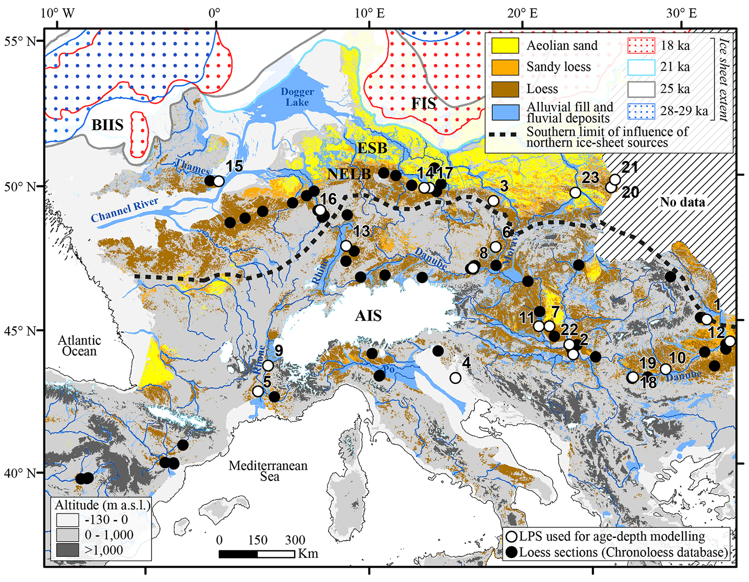
Figure 1 Palaeogeographic map of European aeolian deposits from Bertran et al. (2021), showing the location of the LPSs used in the ChronoLoess database and those used for age–depth calculation. The British–Irish ice sheet (BIIS) and Fennoscandian Ice Sheet (FIS) are from Hughes et al. (2016). The Alpine Ice Sheet (AIS) and other LGM glaciers are from Ehlers and Gibbard (2004). The −130 m coastline is from Zickel et al. (2016). The map is based on the ETOPO1 digital elevation model (Amante and Eakins, 2009). The list of sites used for age–depth modelling are as follows: 1: Balta Alba Kurgan; 2: Batajnica; 3: Biały Kościół; 4: Bok; 5: Collias; 6: Dolní Vĕstonice; 7: Dunaszekcső; 8: Krems-Wachtberg; 9: Lautagne; 10: Lunca; 11: Madaras; 12: Mircea Vodă; 13: Nussloch; 14: Ostrau; 15: Pegwell Bay; 16: Schwalbenberg II; 17: Seilitz; 18: Slivata 1; 19: Slivata 2; 20: Strzyżów; 21: Tyszowce; 22: Veliki Surduk; and 23: Złota.

2 Methods

2.1 Chronological data

2.1.1 ChronoLoess database

In the present study, we have collected luminescence ages from 77 publications in a database called the “ChronoLoess database”, including 93 LPSs from 16 European loess regions (Fig. 1). The data were selected according to the following two criteria: (1) only papers published after the year 2000 were used, and (2) only loess deposits accumulated during the Last Glacial were considered. In 2000, the single-aliquot regenerative-dose (SAR) protocol for OSL (Murray and Wintle, 2000) on quartz and IRSL measurements on feldspar (Wallinga et al., 2000) was introduced. In conjunction with the advent of automatized instruments (e.g. Bøtter-Jensen et al., 1999; Duller et al., 1999a, b), those developments mark significant steppingstones on the way to the success of luminescence dating in Quaternary sciences, and the following homogenization of protocols and measurement equipment also makes luminescence ages better comparable.

A total of 1423 luminescence ages from quartz, feldspar, or polymineral fractions were used. We did not use published ages, but we manually extracted numerical parameters from the original papers such as radionuclide concentrations or equivalent doses; we compiled them in MS Excel™ and recalculated the ages with the dose rate and age calculator DRAC (v.1.2, Durcan et al., 2015) (see Sect. 2.1.2 for more details).

We provide this database in version 1.0.0 as *.xlsx and *.csv file formats via Zenodo (Bosq et al., 2023) to make it available to the scientific community. This database is meant to receive rolling updates in the future, including more recent age data.

2.1.2 Recalculating published luminescence ages

While some isolated recommendations exist for reporting luminescence data (e.g. Duller, 2008; Bateman, 2019; DKE/K 967, 2022; Mahan et al., 2022), those are seldom followed. Similarly, software tools used to analyse data and calculate ages often remain unreported (for a discussion, see Kreutzer et al., 2017). This situation puts up a barrier that severely impedes the recycling and comparison of luminescence age records and is further complicated by the number of single parameters to consider for age calculation. Unfortunately, there is no simple way to circumnavigate this issue and tap into the otherwise excellent and unique chronological datasets covering mainly the Late Pleistocene. In order to use the published luminescence data in our chronological modelling, we made a couple of processing decisions as outlined in the following.

1. As mentioned in Sect. 2.1.1, we did not use published ages but extracted numerical quantities published along with the ages, such as radionuclide concentrations. This decision allowed us to cancel out systematic deviations between datasets resulting from, for example, age calculation software tools and applied dose-rate conversion factors.

2. We treated most datasets reporting infrared-stimulated luminescence (IRSL, including IRSL data after different thermal treatments, so-called post-IR IRSL data) as minimum ages to avoid incorporating potential systematic errors from fading corrections (cf. King et al., 2018) and measurements of the fading rate itself. Higher signal stability was reported for ages derived from post-IR IRSL at 290 ^∘C measurements (e.g. Buylaert et al., 2012), and studies often assumed negligible fading or reported inconclusive results that allowed the authors to circumvent a fading correction. Residual doses, as far as reported, were not subtracted (we refer the reader to the database for details on selected and discarded datasets).

3. We recalculated all cosmic and environmental dose rates using DRAC (v.1.2, Durcan et al., 2015). The external Rb concentration was always calculated from K. This decision bears the risk that the Rb concentration might not best reflect the true Rb concentration in all cases (cf. Mejdahl, 1987; Huntley and Hancock, 2001; Buylaert et al., 2018). However, we decided to follow Mejdahl's conclusion that in the absence of measured Rb values, which was the case for all studies except for Fenn et al. (2020), a calculation of Rb from K is still better than not having taken Rb into account.

   In rare cases, the original study did not report sufficient information but provided only processed data for cosmic and environmental dose rates, and the data could not be recalculated.

4. Except for rare cases of apparent mistakes (for instance, typos), other parameters combined with high degrees of freedom (e.g. alpha efficiency, internal dose rates, measurement protocol parameters, statistical data treatment) were always taken as reported by the study's authors. Missing or faulty units and citations (e.g. obviously unsuitable reference) were not considered errors if these data appeared meaningful otherwise.

5. The final age uncertainties do not include systematic uncertainties, except those already part of tabulated values.

In other words, we placed wagers on the authors' knowledge and insight, making expert decisions on individual parameters, which includes fundamental decisions such as the chosen mineral and grain size fraction or the method to estimate radionuclide concentrations. When an original study (including supplements) did not provide sufficient information to recalculate the luminescence ages in sporadic cases, such results were considered non-reproducible and discarded. For the list of parameter selections, we refer to Table S1 in the Supplement.

Our selection remains imperfect without accessing and reanalysing primary data (e.g. *.bin or *.binx files containing luminescence measurements). However, such data are usually unavailable without contacting study authors on a case-to-case basis. Still, the amount of pooled data likely leads to averaging effects in the case of extreme values, providing sufficient statistical confidence in the modelling results. In the following, all ages are reported in kiloyears before 2000 (b2k).

2.1.3 Calculation of time–activity curves

In our results, we will present time–activity curves. The time–activity curve characterizes the rate of events over time. It gives the number of events (here, the number of dated dust accumulation events) that have occurred per unit of time. It is also called the cumulative probability density function (CPDF) because it is equal to the probability density (or probability distribution) of events over time multiplied by the total number of dates n. Different approaches to estimating this activity curve have been proposed and discussed in the literature, mainly based on the histogram method (Vermeesch, 2012) or density estimation by kernel methods (Vermeesch, 2012; Contreras and Meadows, 2014; Bronk Ramsey, 2017). However, these methods do not take into account errors on dates and do not allow for the calculation of an error envelope on the estimated density. This is why we propose to estimate this density by the sliding window method, which uses a uniform kernel of width h (Rivoirard and Stoltz, 2012; Lanos and Dufresne, 2022). In this case, the number of events that occur in a window of width h centred on a time θ is a random variable denoted A(θ,h) that follows a binomial distribution of n parameters (the total number of dated events) and q(θ) which represents the theoretical proportion of events that occur in the considered window. From this binomial probability law, we can deduce the average activity or expectation (here noted E[.]) of the number of events per unit of time, i.e.:

$$\begin{array}{}\text{(1)}& E\left[A\left(\mathit{\theta },h\right)\right]=n{\displaystyle \frac{q\left(\mathit{\theta }\right)}{h}}.\end{array}$$

The parameter q(θ) is unknown; it is then estimated from the observed frequency f_n(θ), which is equal to the number n_i of dates observed in the window of width h centred on θ, divided by the total number of dates n. Since each date is affected by an uncertainty represented by a probability density, the contribution of a date to a given window will therefore be given by the probability that the date appears in the window interval. This value is between 0 (the date is not in the window) and 1 (the whole date distribution is in the window). This probability can be easily obtained by a large number of Monte Carlo draws from the date distribution. Ultimately, the observed frequency for the window of width h centred on θ will be given by the sum of the probabilities of the dates belonging to the window divided by the total number of dates. Because of the binomial distribution and from the observed frequency f_n(θ), it is possible to estimate the parameter q(θ) by an interval q₁(θ) and q₂(θ) at a 95 % confidence level. This interval is obtained using the Clopper and Pearson (1934) chart. The 95 % confidence interval (or error envelope) on the activity curve is derived by

$$\begin{array}{}\text{(2)}& n{\displaystyle \frac{q_{\mathrm{1}}\left(\mathit{\theta }\right)}{h}}\le A\left(\mathit{\theta },h\right)\le n{\displaystyle \frac{q_{\mathrm{2}}\left(\mathit{\theta }\right)}{h}}.\end{array}$$

The average activity E[A(θ,h)] is estimated by the expression

$$\begin{array}{}\text{(3)}& n{\displaystyle \frac{f_n\left(\mathit{\theta }\right)}{h}}.\end{array}$$

It is important to note that this is a point confidence interval, i.e. estimated at each point θ independently of the other points, and not a confidence band, i.e. of uniformity in θ (Rivoirard and Stoltz, 2012).

2.1.4 Comparison of the observed activity curve with the assumption of a uniform random distribution of dates

The question may arise whether the peaks or troughs observed on the activity curve are statistically significant for the assumption of a uniform random distribution of dates in the period considered. In the case where all dates are uniformly distributed between dates θ_m and θ_M, the date probability density becomes $q\left(\mathit{\theta }\right)=\frac{h}{({\mathit{\theta }}_M-{\mathit{\theta }}_m)}$. This is represented by a rectangular graph of width (θ_M−θ_m) and height q(θ). If this uniform distribution lies within the envelope of the 95 % activity curve, this means that the peaks or troughs of the curve may not be significant; that is, they may be the result of a uniform random distribution of dates.

Another aspect to discuss is the choice of the width h of the window. Given the geological problem posed, the idea here is to vary the width h to maximize the gap between the two curves, accounting for the error envelope. If a peak or trough, with its 95 % error envelope, does not contain the uniform distribution, we can calculate a deviation which, summed over all the dates θ according to a fine exploration step, defines a global significance score S_h as a function of h. This score is analogous to a distance in total variation between two probability distributions (Rivoirard and Stoltz, 2012), but here we take into account the 95 % error envelope. The calculation of the activity curve is implemented in the chronological modelling application ChronoModel v2.0 (Lanos and Philippe, 2017a, b; Lanos and Dufresne, 2019), and the new ChronoModel v3.0 (Lanos and Dufresne, 2022) allows for calculating the S_h score as a function of h. The width h that maximizes this score is sought. The width h thus determined indicates the resolution on the date θ of a peak or trough, which does not contain the uniform distribution in its envelope. The idea of maximizing the S_h score emanates from the geological problem posed: we want to know if dated events are more frequent at certain periods than at others. We, therefore, search for the window width h that best highlights this deviation from date uniformity. Note that using a uniform kernel of width h (sliding window) necessarily produces an edge effect at the data's extremities (θ_m,θ_M). This is why we replace the rectangular distribution by a “trapezoid” distribution to correct this effect and allow for comparison (the calculation of the significance score) with the activity curve.

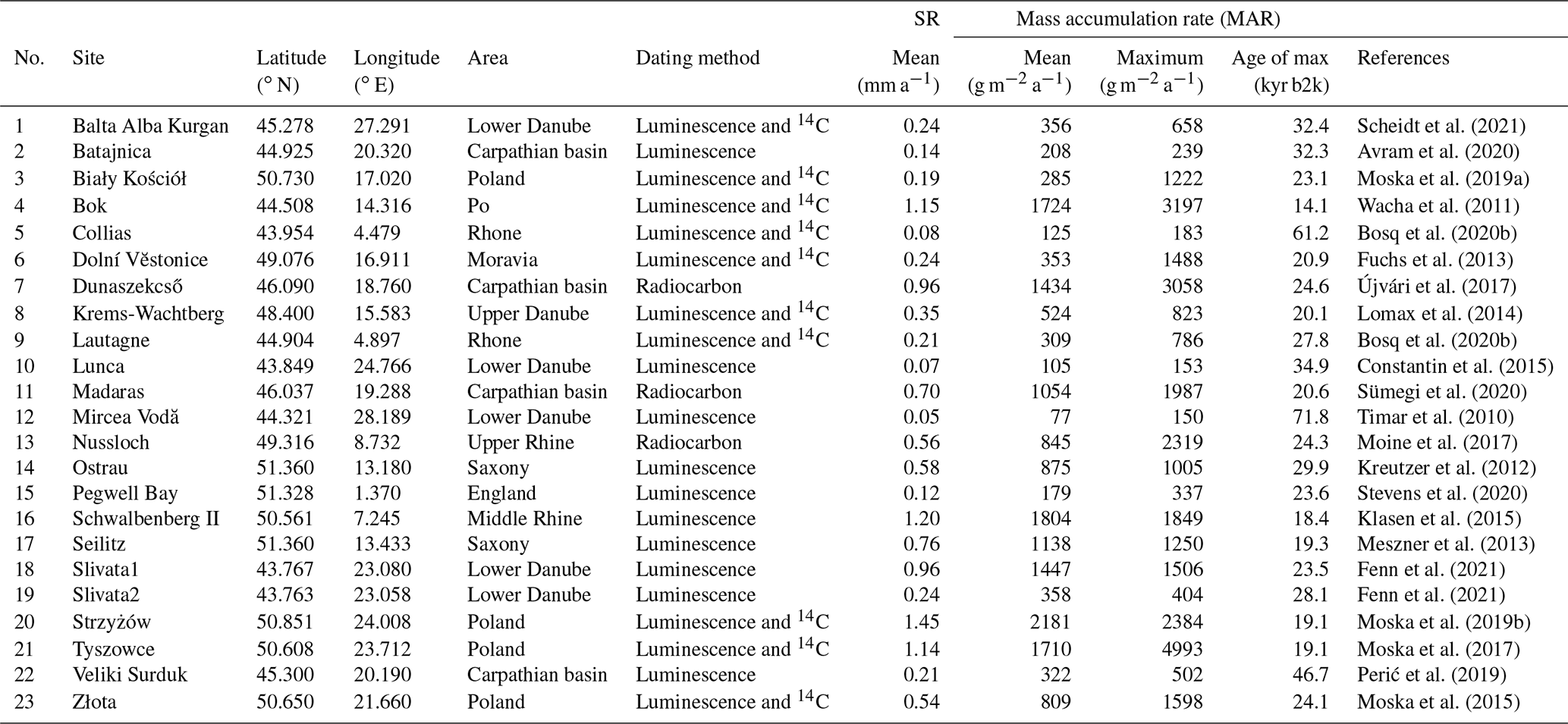
Table 1 Average sedimentation rate (SR) and mass accumulation rate (MAR) from Bayesian age–depth modelling of 23 LPSs during the last 60 kyr b2k. Data sources: Balta Alba Kurgan (Scheidt et al., 2021); Batajnica (Avram et al., 2020); Biały Kościół (Moska et al., 2019a); Bok (Wacha et al., 2011); Collias (Bosq et al., 2020b); Dolní Vĕstonice (Fuchs et al., 2013); Dunaszekcső (Újvári et al., 2017); Krems-Wachtberg (Lomax et al., 2014); Lautagne (Bosq et al., 2020b); Lunca (Constantin et al., 2015); Madaras (Sümegi et al., 2020); Mircea Vodă (Timar et al., 2010); Nussloch (Moine et al., 2017); Ostrau (Kreutzer et al., 2012); Pegwell Bay (Stevens et al., 2020); Schwalbenberg II (Klasen et al., 2015); Seilitz (Meszner et al., 2013); Slivata 1 (Fenn et al., 2021); Slivata 2 (Fenn et al., 2021); Strzyżów (Moska et al., 2019b); Tyszowce (Moska et al., 2017); Veliki Surduk (Perić et al., 2019); and Złota (Moska et al., 2015).

2.2 Bayesian age–depth modelling

2.2.1 Data selection

Bayesian age–depth modelling was performed on a limited number of LPSs (n=23) (see Table 1). The chronological models take into account both the recalculated luminescence ages (extracted from the ChronoLoess database) and accelerator mass spectrometry (AMS) radiocarbon ages when available (see Fig. S2). Only LPSs with more than six luminescence and/or radiocarbon ages were retained. The published AMS radiocarbon ages were obtained from various materials, including charcoal fragments, gastropod shells, and calcitic earthworm granules. Conventional radiocarbon ages were calibrated to calendar ages with the IntCal20 calibration curve (Reimer et al., 2020) using ChronoModel v3.0 (Lanos and Dufresne, 2022).

2.2.2 Overview of the method used in ChronoModel

The estimate of MARs is based on the building of age–depth curves. For this purpose, we used a Bayesian approach developed by Philippe Lanos in RenCurve (Lanos, 2004); it is now implemented in the new version of ChronoModel v3.0 (Lanos and Dufresne, 2022). The Bayesian approach makes it possible to estimate a mean age–depth curve with its confidence envelope that interpolates the data and takes into account the uncertainties coming from the chronometric dates and errors in depth measurements (mostly small). Additional individual errors (so-called irreducible errors) are respectively added on the dates and depths to take into account the possible presence of outlying dates and stratigraphic inversions. This Bayesian modelling, therefore, automatically penalizes the influence of outliers. The curve estimation itself is based on a penalized cubic spline function, which aims to realize a compromise between smoothing and fitting at the data points (age–depth), thanks to a smoothing parameter estimated using Bayesian modelling. It is important to note that the cubic spline works similarly to a kernel method: the thinner the bandwidth, the greater the point density over time (Green and Silverman, 1993). In other words, the smoothing adapts locally to the point density. The numerical calculation is carried out using Markov chain Monte Carlo (MCMC) techniques (Metropolis–Hastings algorithm) (Gilks et al., 1995) implemented in ChronoModel. For each age–depth sequence, 300 000 iterations were needed to obtain a precise estimation of the mean curve, its error envelope, the posterior irreducible variances (on time and depth), and the smoothing parameter. From the obtained age–depth curve, we can estimate the rate of loess accumulation, which is given by the first derivative of the mean curve at each time.

Figure 2 Example Bayesian age–depth model of Balta Alba Kurgan LPS from ChronoModel.

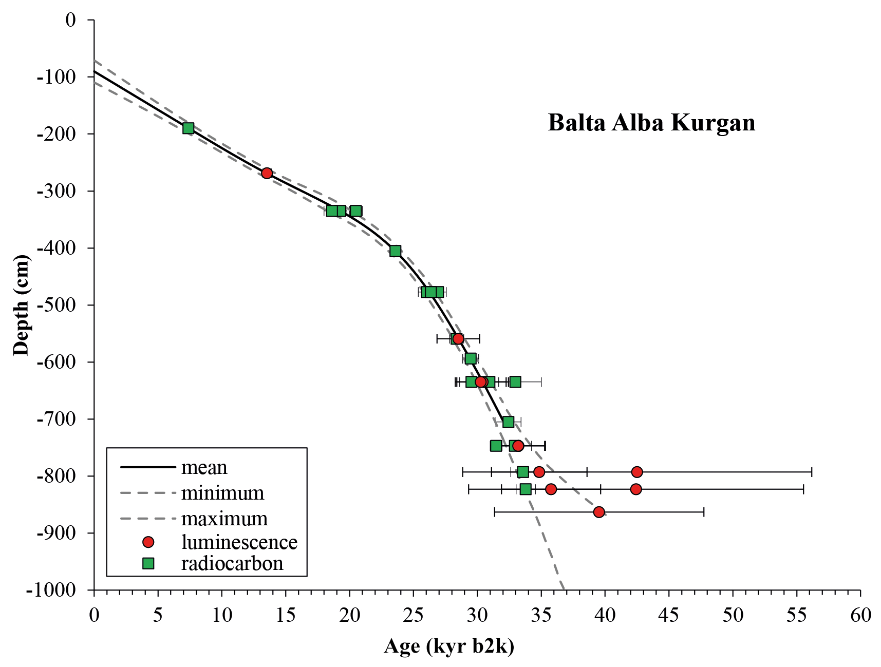
An example of an age–depth curve is shown in Fig. 2 (Balta Alba Kurgan), where dates have been determined by ¹⁴C (green squares) and luminescence dating (red dots). Each point (square or dot) corresponds to the middle of the date interval at 95 %, represented by a horizontal bar. Some depths are dated several times by ¹⁴C and/or luminescence. The date intervals can therefore overlap for the same depth. We note in this example that some of the luminescence dates at the bottom are considered outliers and penalized during the mean curve calculation. This explains why the error envelope on the depth is more significant in this part.

2.2.3 Mass accumulation rates (MARs)

Reconstructing MARs is essential for a reliable picture of past dust deposition and comparison of loess records from different regions and for understanding and estimating past atmospheric mineral dust activity (Albani et al., 2015). This work requires independent and accurate high-resolution age–depth models. Therefore, based on the Bayesian age–depth models performed as part of this study (see the previous paragraph), we calculated the MARs for each LPS using the following equation proposed by Kohfeld and Harrison (2003):

$$\begin{array}{}\text{(4)}& \text{MAR}\left(\mathrm{g}{\mathrm{m}}^{-\mathrm{2}}{\mathrm{a}}^{-\mathrm{1}}\right)=\text{AR}\times f_{\mathrm{eol}}\times {\mathit{\rho }}_{\mathrm{dry}},\end{array}$$

where AR is the bulk accumulation rate (m a⁻¹), f_eol is the sediment fraction aeolian in origin (we assumed here to be 1), and ρ_dry is the bulk density of dry sediment (g m⁻³). Estimated bulk density values for loess vary in the literature and between loess regions (Frechen et al., 2003; Kohfeld and Harrison, 2003; Újvári et al., 2010). Here, we adapted a bulk density value of 1.5 g cm⁻³ for our calculations based on the average loess values from the European region (Újvári et al., 2017; Perić et al., 2019; Fenn et al., 2020). For each LPS, mean MARs were calculated from the following formula:

$$\begin{array}{}\text{(5)}& \text{MAR}\left(\mathrm{g}{\mathrm{m}}^{-\mathrm{2}}{\mathrm{a}}^{-\mathrm{1}}\right)=\left({\displaystyle \frac{{\text{depth}}_{\mathrm{2}}-{\text{depth}}_{\mathrm{1}}}{{\text{age}}_{\mathrm{2}}-{\text{age}}_{\mathrm{1}}}}\right)\times f_{\mathrm{eol}}\times {\mathit{\rho }}_{\mathrm{dry}}\end{array}$$

where depth₁ and depth₂ are the depths of the highest and lowest dated samples in the loess profile, respectively, and age₁ and age₂ are the modelled ages for the corresponding depths. This calculation avoids the high uncertainties associated with the ends of each age–depth model.

The dating resolution has an impact on the calculated MARs. This is particularly true for extreme MARs, i.e. the highest values for a given sequence. Long intervals between dates necessarily result in averaging MARs over the considered period. In this study, the chronological models consider the recalculated luminescence ages (extracted from the ChronoLoess database) and AMS ¹⁴C ages where available. Many dates are available for the periods of greatest dust accumulation in most sequences; for example, nine levels have been dated for the Balta Alba Kurgan LPS between 35 and 24 kyr b2k and up to 13 levels for the Biały Kościół LPS between 28 and 20 kyr b2k. We consider the extreme MAR values obtained as representative, although we acknowledge that we cannot exclude that their exact timing might partly suffer from a dating-resolution-related inaccuracy.

3 Results

3.1 ChronoLoess database: first results

In this study, we started with 1423 recalculated luminescence ages. The quality of the data was estimated from the comparison of the ages reported in the original studies and the ages recalculated using DRAC. We considered age discrepancies of less than 10 % as acceptable, while larger discrepancies were considered errors requiring additional inspection or correction. As quality control, we randomly sampled 100 ages, which yielded reasonable age differences between 0.2 % and 20 % (see the Supplement for more details and Fig. S1). Some ages (n=7) showed a discrepancy of >20 %, which usually indicated input errors in the DRAC table, such as missing information or wrong input dimensions. We corrected those errors (which were then usually found in other datasets) and now assume that >95 % of the data in the dataset are free of copy errors. In some cases, it turned out that the original study (and supplements) did not contain enough information to recalculate the ages. Thus, 247 ages were not included and were considered incorrect, non-reproducible, or repetitions (typically if different luminescence protocols were tested in a study). In addition, we focused only on a study period ranging from 60 kyr b2k to the present, eliminating 205 additional ages. Nevertheless, some of these older ages were used in the generation of age–depth models (see Sect. 3.2). This selection finally left us with 971 ages extracted from the database available for the analysis of loess deposition.

The ages obtained are unevenly distributed in 16 loess regions: southern England (n=20); northern France/Belgium (n=42); Saxony (Germany) (n=55); southern Poland (n=134); upper Rhine (upstream of Mainz) (n=46); middle Rhine valley/Lower Rhine Embayment (middle/lower Rhine) (n=101); Harz (Germany) (n=19); upper Danube (n=75); Carpathian basin (middle Danube) (n=188); lower Danube (n=143); Dniester (n=21); Prut (n=18); Moravia (n=20); Po (n=47); Rhone (n=19); and Ebro/Tajo (n=23). In regions where the number of ages selected is greater than 100 (e.g. Carpathian basin, middle Rhine valley/Lower Rhine Embayment, Poland), representativeness is assumed to be acceptable. Results from other regions (n≤100) should be considered cautiously. These regions account for the majority of our dataset. Therefore, the recalculated ages were grouped into two sets corresponding to the main European loess regions, the Northern European Loess Belt (NELB) (n=371) and the Perialpine Loess (PL) (n=517) (see Fig. 1 for the approximate boundary). Such a grouping avoids statistical under-representation for some regions and minimizes the importance of local peculiarities, particularly the problems related to erosional phases in the LPS. Data from continental aeolian deposits disconnected from the main ice sheets, such as the Dniester, Prut, Tajo, and Ebro basins as well as the Moravia region, were excluded from our compilation due to the low number of ages available. As mentioned above, these aeolian systems are likely to provide a record different from the NELB and PL (e.g. Wolf et al., 2018) and would deserve to be dated more widely.

The two large groups correspond to distinct and relatively homogeneous aeolian systems. The NELB is a band of loess that developed south of the European Sand Belt (ESB; Zeeberg, 1998). It stretches in low-relief areas between latitudes 48^∘ N and 51^∘ N approximately, from the tip of Brittany to the east of Poland (Fig. 1). The grain size distribution shows a gradual transition from coversands to sandy loess and loess (Bertran et al., 2021; Lehmkuhl et al., 2021). This grain size gradient is controlled by the distance to the glaciofluvial sources and topography in a context of low and sparse vegetation (tundra–steppe). This pattern and the chemical composition of loess, which is rich in potassic minerals and relatively poor in carbonates (Bosq et al., 2020a; Skurzyński et al., 2020), i.e. close to the composition of the felsic rocks of the Scandinavian shield, suggest a common supply predominantly from the outwash plains of the FIS. Mixing with local sources also influenced the chemical and mineralogical composition, explaining minor regional differences (Baykal et al., 2021). PL accumulated, often with marked asymmetry, along large rivers fed by the AIS (Danube, Po, Rhone, Rhine) (Fig. 1) and is characterized by a relatively homogeneous chemical composition, with a high carbonate content due to the abundance of calcareous rocks in the bedrock of the AIS (Buggle et al., 2008; Újvári et al., 2008; Bosq et al., 2020a). The coarse texture, poor grain size gradient, and more variable thickness make it distinct from northern European loess. It has been suggested that capturing particles transported by saltation and short-term suspension by dense, shrubby vegetation typical of southern areas was the main factor in the dominant accumulation of coarse loess close to fluvial sources (Bosq et al., 2018; Bertran et al., 2021).

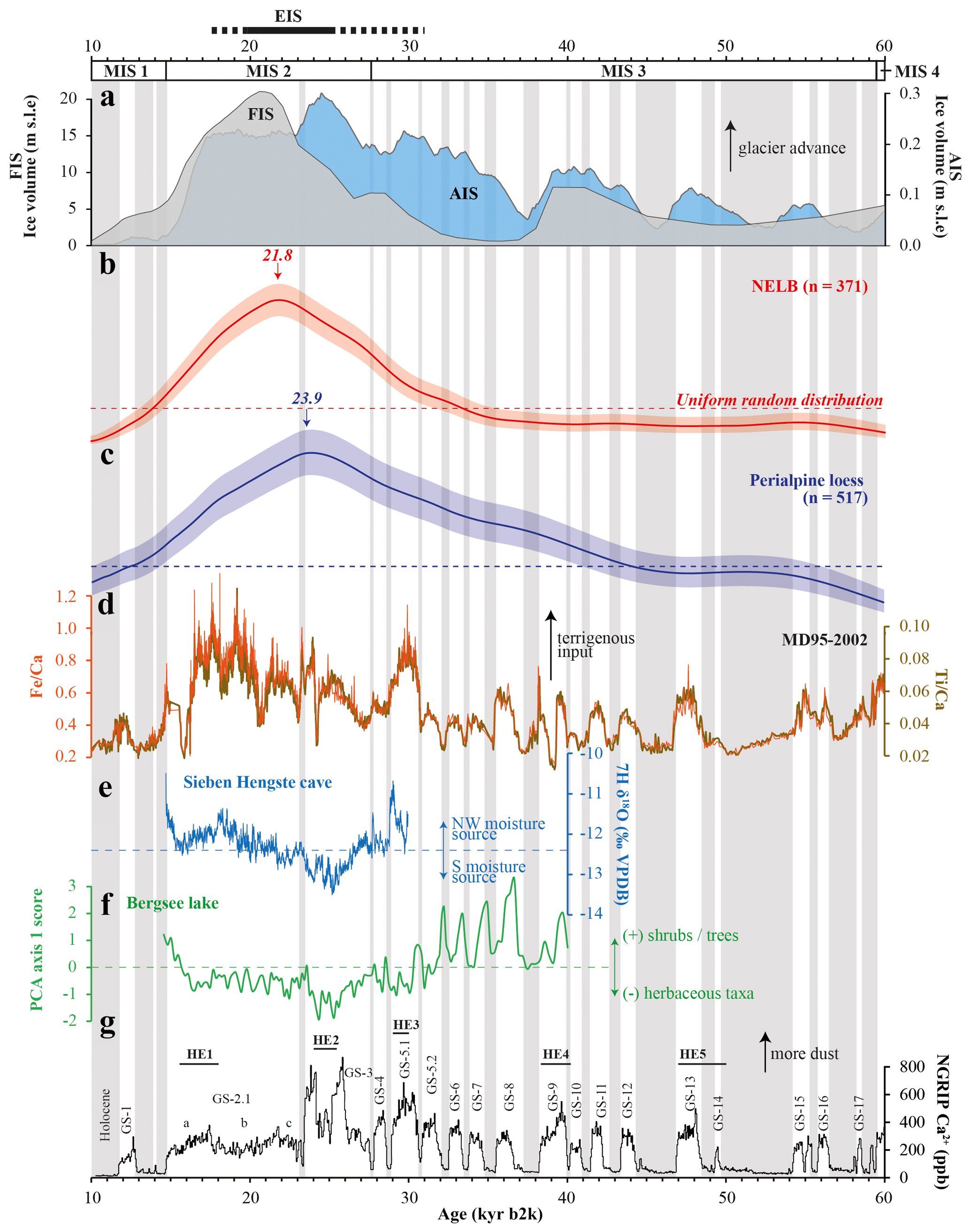
Figure 3 Comparison between ice and sediments records. (a) AIS and FIS ice volumes between 60 and 10 kyr b2k are from simulations (Seguinot et al., 2018; Lambeck et al., 2010). Modelled ice volumes are expressed in metres sea-level equivalent (m s.l.e.). (b, c) Time–activity curves for the NELB (red) and perialpine loess (blue) are shown; the coloured bands indicate the 95 % confidence interval, and the dotted lines indicate the uniform random distribution. (d) $\mathrm{Fe}/\mathrm{Ca}$ and $\mathrm{Ti}/\mathrm{Ca}$ ratios are from the MD95-2002 core off Brittany (Toucanne et al., 2015, 2021). (e) Sieben Hängste (7H) composite stalagmite δ¹⁸O record (western Alps) (Luetscher et al., 2015). (f) Score of principal component analysis (PCA) axis 1 for pollen data from Bergsee (south Germany) (Duprat-Oualid et al., 2017). (g) North Greenland Ice Core Project (NGRIP) Ca²⁺ data over the last 60 kyr b2k (Rasmussen et al., 2014). The marine isotope stage (MIS) and Heinrich events (HEs) are from Sanchez Goñi and Harrison (2010).

The age distribution of loess in these two areas is used here to indicate the aeolian dynamics over the last 60 millennia. It is represented by the activity curve and its 95 % confidence interval (Fig. 3). Maximum age densities (i.e. clusters) with its confidence envelope are shown as peaks exceeding the line representative of a uniform random distribution. These density maxima provide a chronological estimate of the main periods of dust accumulation. The bandwidth chosen in the following discussion was calculated to maximize the significance score, i.e. 8.1 kyr for the NELB and 9.7 kyr for PL.

At the continental scale, the comparison between the two areas highlights the following points (Fig. 3):

1. The age distribution is not uniform over time, and clusters are clearly identifiable. These clusters reflect episodes of intense aeolian accumulation and cover a time interval encompassing the Weichselian Upper Pleniglacial (approximately MIS 2), which coincides with the maximum advance of European glaciers (Fig. 3a). For older periods and the early Holocene, the age density is low and lies below the uniform distribution line. This indicates little to no aeolian sedimentation.

2. Substantial loess deposition in the NELB started several millennia later than in the perialpine aeolian systems. In the former area, dust accumulation increased from about 32 kyr b2k, i.e. from Greenland Stadial (GS)-5.2 (Rasmussen et al., 2014), and rose steeply after 30 kyr b2k, i.e. during GS-5.1 (Fig. 3b). In contrast, deposition in the perialpine area started earlier and increased as early as 42 kyr b2k (GS-11), with a further rise after 40 kyr b2k (GS-9) (Fig. 3c). Although the chronological limits of Heinrich events (HEs) remain relatively imprecise, GS-5.1 and GS-9 correlate with HE-3 and HE-4, respectively, in marine records (Sanchez Goñi and Harrison, 2010).

3. For the PL, deposition peaked at 23.9 kyr b2k (Fig. 3b), i.e. at the very end of GS-3 (HE-2). The age distribution in the NELB contrasts with that of the perialpine loess. Dust accumulation peaked during the LGM at 21.8 kyr b2k (GS-2.1c) and then decreased sharply at the end of GS-2.1 (Fig. 3c). For both aeolian systems, the large bandwidth chosen (together with the uncertainty associated with the luminescence ages) and the variability related to local factors do not allow for the identification of well-defined secondary peaks within the main accumulation period.

4. When splitting the NELB data into two subsets, the eastern part (here referred to E-NELB, i.e. Poland, eastern Germany, n=208) and the western part (W-NELB, France, England, Belgium, western Germany, n=163) show contrasting activity curves. W-NELB shows a plateau between 26.5 and 20.5 kyr b2k, while E-NELB has a bell shape centred at 21.7 kyr b2k (Fig. 4). Loess deposition thus appears to have started significantly earlier in the BIIS-influenced part of the NELB, and the peak accumulation lasted longer.

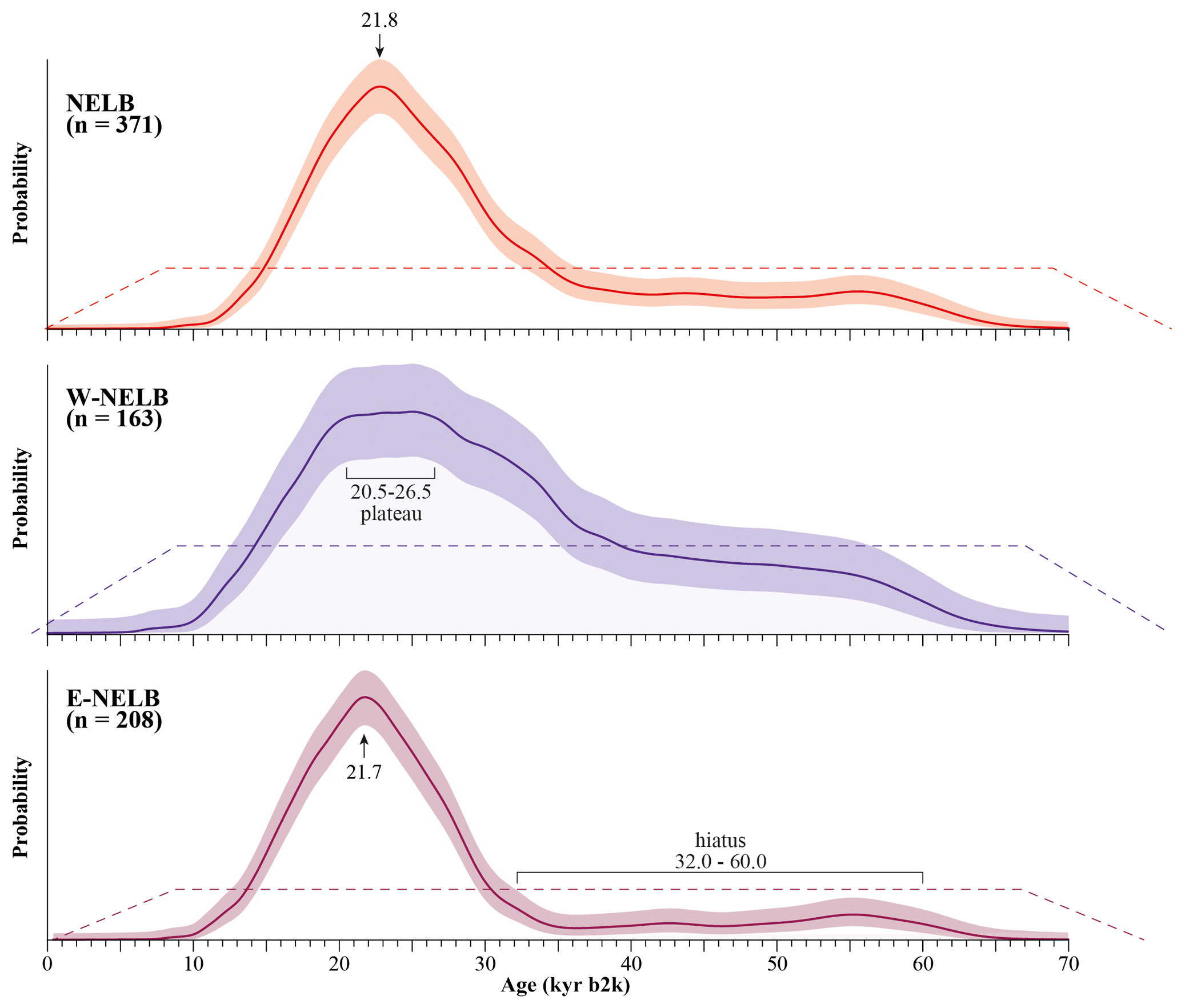
Figure 4 Time–activity curves for the NELB, W-NELB (Belgium, southern England, northern France, western Germany), and E-NELB (southern Poland, eastern Germany). The coloured bands indicate the 95 % confidence interval, and the dotted lines indicate the uniform random distribution.

3.2 Mass accumulation rates

The spatial distribution of the LPS used to build the Bayesian age–depth models is shown in Fig. 1, while the sites studied are listed in Table 1. The chronological models take into account both the recalculated luminescence ages (extracted from the ChronoLoess database) and AMS ¹⁴C ages when available. The distribution of sites does not appear spatially homogeneous, with notably a lack of well-dated LPSs in the western part of the NELB (northern France, Belgium) and a deficit in the Po plain and the upper Danube. These differences do not correspond to a field reality (lack of available sections) but reflect the current state of research. Nevertheless, while awaiting further dating work, the number of age–depth models produced in this study (n=23) allows for discussion of sediment accumulation rates at a pan-European scale.

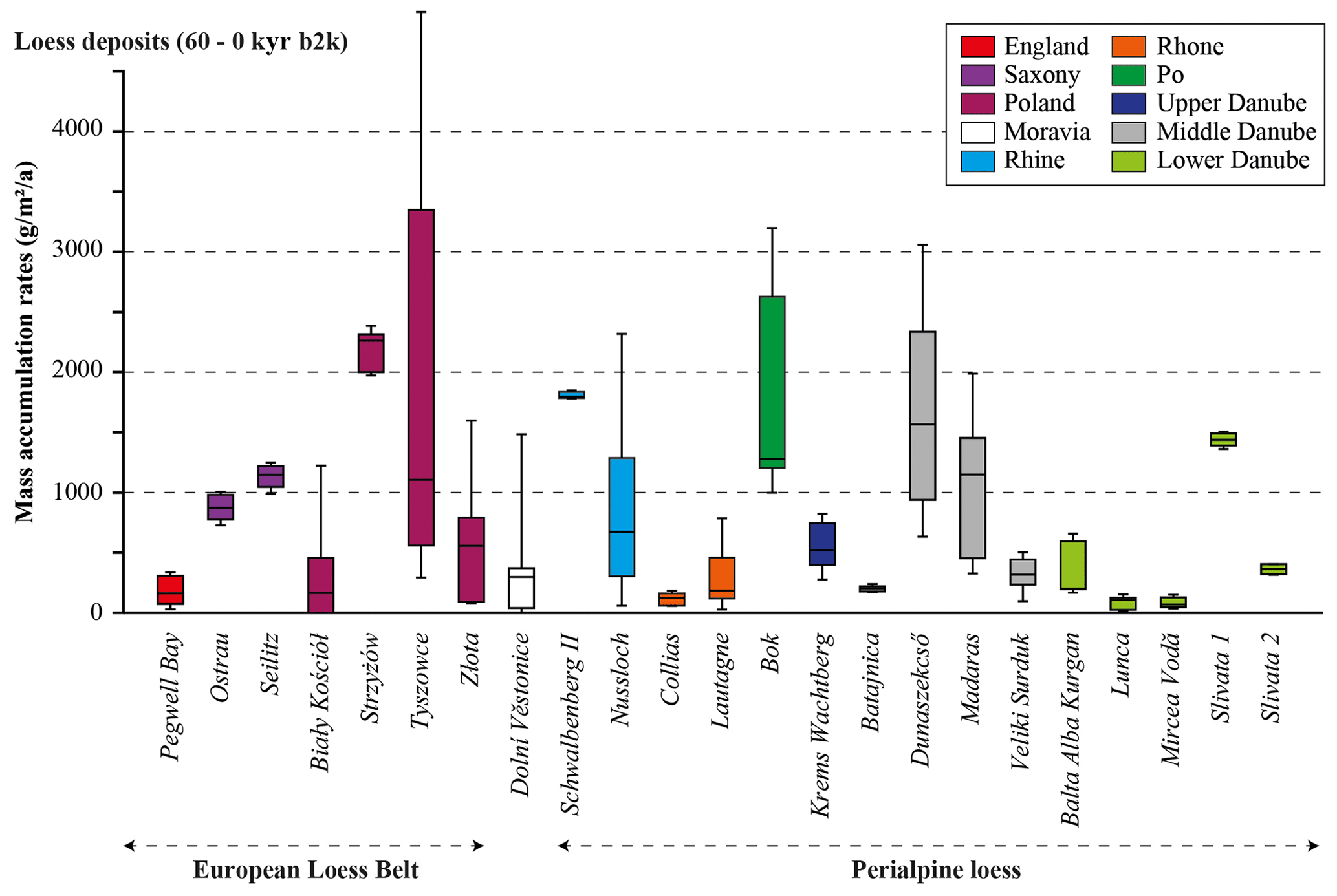
Figure 5 Box plot of MARs derived from age–depth modelling of some European LPSs between 60–0 kyr b2k (references in Table 1).

During the study period (60–0 kyr b2k), the mean sedimentation rates derived from Bayesian age–depth models vary between 0.05 and 1.45 mm a⁻¹, while the mean MARs range from 77 to 2181 g m⁻² a⁻¹, with extreme MAR values of 150 g m⁻² a⁻¹ and 4993 g m⁻² a⁻¹ (Table 1). Figure 5 shows a large variability of MARs between regions but also between sites within the same region, with MARs varying by an order of magnitude. We found the highest dust accumulation rates in Poland and in the Po and Rhine valleys, and we observed the lowest fluxes in England and the lower Danube. MARs also varied strongly over time (Figs. 5, S3). Age models based on radiocarbon dating show multiple peaks (e.g. Dunaszekcső, Madaras Nussloch) and better resolution compared to models using luminescence ages, which tend to smooth the curves (Fig. S2).

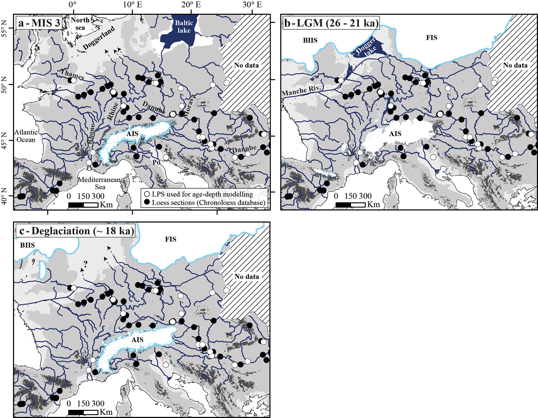
Figure 6 Palaeogeographic maps of Europe. (a) 38–35 ka time slice (GI-8, GI-7); the Baltic lake is from Lambeck et al. (2010). (b) 26–21 ka time slice. (c) ca. 18 ka. The sea levels are from Lambeck et al. (2014).

4 Discussion

4.1 Impact of ice sheets on aeolian dynamics

As previously demonstrated in many studies and despite chronological uncertainties, the bulk of loess accumulation occurred during MIS 2 (Antoine et al., 2009; Stevens et al., 2011; Guérin et al., 2017; Újvári et al., 2017; Zens et al., 2018; Moska et al., 2019b; Stevens et al., 2020; Perić et al., 2022). Our results unambiguously indicate that the main phase of accumulation occurred later for the NELB than for the PL. This phase started at about 32 kyr b2k for the NELB vs. 42 kyr b2k for PL and peaked about 2 millennia later for the former (21.8 vs. 23.9 kyr b2k, respectively). In agreement with Kocurek and Lancaster (1999), several factors may have influenced this time lag, such as (i) the amount of fine particles released by their respective sedimentary sources, (ii) the wind transport capacity, and (iii) the local availability of sediments (role of vegetation and soil moisture). Among the various potential factors, fluctuations in the amount of particles available for deflation due to changes in ice sheet pattern appear to be a pivotal point that explains the chronological disparities between aeolian systems. For northern Europe, reconstructions show the following:

1. During late MIS 3 (∼35 kyr b2k, GI-7), the area covered by the FIS was restricted to the Norwegian mountains (Hughes et al., 2016). During this period, sediment produced by glacial abrasion was transported by meltwater to a proglacial lake, the Baltic lake (Lambeck et al., 2010) (Fig. 6a). A significant portion of the dust from the outwash was trapped by the lake. This pattern could explain the near absence of deposition in the E-NELB between ∼60 and 32 kyr b2k (Figs. 3b, 4) and strengthens the ∼30 kyr hiatus hypothesis for LPSs of Saxony suggested through high-resolution luminescence dating (Kreutzer et al., 2012; Meszner et al., 2013; Meszner and Faust, 2014). Simultaneously, the considerable growth of the BIIS (Clark et al., 2022) resulted in significant loess deposition in the W-NELB (Fig. 4).

2. During MIS 2, the BIIS and FIS invaded the North Sea basin and merged into a single ice sheet, the European Ice Sheet (EIS) (Clark et al., 2012; Hughes et al., 2016; Batchelor et al., 2019) (Fig. 6b). Recent reconstructions of the ice extent in the North Sea suggest a coalescence of the BIIS and FIS at ca. 26 ka (e.g. Becker et al., 2018; Roberts et al., 2018; Clark et al., 2022). Coalescence resulted in the rerouting of meltwater produced by the FIS toward the North Atlantic via the Channel River, which then served as the primary drain for proglacial flows and for the Rhine, Seine, and Thames rivers (Toucanne et al., 2015; Patton et al., 2017). Analysis of the MD95-2002 marine core collected at the foot of the continental slope off Brittany indirectly allows for dating the beginning of the development of the Channel mega-catchment (Toucanne et al., 2015). $\mathrm{Fe}/\mathrm{Ca}$ and $\mathrm{Ti}/\mathrm{Ca}$ ratios in sediments, which are proxies for terrigenous inputs, increased abruptly at ca. 31 kyr b2k and kept high values until ca. 16.5 kyr b2k despite some fluctuations (Fig. 3d). The onset of this phase is synchronous with the beginning of loess accumulation in the northern European plain (Fig. 3b) and the establishment of cold and relatively dry conditions on the European continent recorded by pollen assemblages (Fletcher et al., 2010; Duprat-Oualid et al., 2017) (Fig. 3f). The maximum of dust sedimentation is then concomitant with the maximal extension of the EIS around 23–21 ka (Hughes et al., 2016; Patton et al., 2016) and reflects the peak of the inputs of glacial particles to proglacial rivers and the Channel River.

3. Between ca. 19.9 and 17.5 ka, the rapid retreat of the ice sheet resulted in the splitting of the BIIS and the FIS (Fig. 6c) (Becker et al., 2018; Evans et al., 2021). Catastrophic drainage of the North Sea ice-dammed lake south of the EIS has been dated to ca. 18.7 ka cal BP (Hjelstuen et al., 2018). Much of the meltwater then flowed to the Norwegian Sea through the open gap between the two ice sheets, and the sedimentary load transported by the Channel River decreased drastically, limiting the amount of particles available for deflation in the W-NELB (Baykal et al., 2022). The rapid northward retreat of the FIS synchronously led to a sharp decrease in loess deposits in the E-NELB. For the NELB as a whole, this decrease was particularly significant after 18 kyr b2k (Fig. 3b).

In comparison, palaeogeographic changes related to AIS fluctuations in response to climate change were less drastic than those of the EIS due to the smaller area and topographic constraints (Seguinot et al., 2018). Recent studies show the following:

1. The AIS reached its maximal volume around 26–23 ka, i.e. during GS-3 (e.g. Preusser et al., 2011; Monegato et al., 2017; Ivy-Ochs et al., 2018; Gaar et al., 2019; Braakhekke et al., 2020; Kamleitner et al., 2022), or even earlier in the western Alps, i.e. between 40 and 30 ka (Gribenski et al., 2021). Isotope records from Alpine speleothems (Luetscher et al., 2015) (Fig. 3e) and climate simulations (Del Gobbo et al., 2023) provide evidence for moisture advection from the Mediterranean Sea to the Alps during GS-3, leading to rapid ice sheet growth. This stadial broadly corresponds to the coldest phase of the Last Glacial (e.g. Hughes and Gibbard, 2015) and coincides with the major peaks of dust accumulation in Greenland ice cores (Ruth et al., 2003; Rasmussen et al., 2014). It also coincides with the accumulation maximum recorded in PL (Fig. 3c).

2. The AIS entered a recession phase after 22 ka and lost approximately 80 % of its ice volume by 17.5 ka (e.g. Ivy-Ochs et al., 2008; Monegato et al., 2017). As a result, the age density of PL decreases sharply during GS-2 (Fig. 3c).

For each of the aeolian systems, the synchrony between loess deposition and the period of maximal glacier advance strongly suggests that the two processes are intimately related. The time lag between the maximal extension of the EIS and AIS, as well as the associated palaeogeographic changes, correctly accounts for the chronological differences between the emplacement of the NELB and PL.

For some authors (Stevens et al., 2020; Baykal et al., 2022), the increase in dust emissions would be largely correlated with the increase in meltwater fluxes during the recession phases of the EIS. Due to the signal smoothing created by the use of a wide bandwidth (imposed by the need to obtain a statistically reliable signal), our approach does not allow us to address this aspect very precisely. The results obtained here nevertheless suggest that, for each aeolian system, the main phase of loess sedimentation corresponded to the maximal advance of the glaciers, while rapid recession ca. 20 kyr b2k led to a marked decrease in accumulation. Observations from contemporary temperate-based glaciers (Hallet et al., 1996; Jansson et al., 2005; Riihimaki et al., 2005) provide some basis for comparison. Overall, fine particle production, primarily by abrasion (e.g. Alley et al., 1997; Iverson et al., 1995; Riihimaki et al., 2005), increases in parallel with glacier size (see the conceptual model of Jansson et al., 2005), due to the larger areas of eroded bedrock and greater amounts of meltwater released in summer. Acceleration of basal slip, caused by increased water pressure in summer, promotes high particle production, which is then discharged into subglacial conduits (Riihimaki et al., 2005). By nature, the accelerated melting of a glacier causes only a transient increase in meltwater flows due to the correlative decrease in the amount of available ice. The geomorphic evolution of the glacier margin also largely influences the downstream transfer of particles (e.g. Knight et al., 2000). Proglacial lakes formed behind moraines and in over-deepened areas during the periods of glacier retreat tend to trap particles and reduce the load carried downstream. However, the periodic drainage of lakes and the redistribution of newly exposed sediments by slope processes introduce significant complexity to the system (e.g. Knight et al., 2000; Porter et al., 2010). In summary, the possibility of a correlation between ice sheet recession and increased loess sedimentation does not seem straightforward and remains to be studied in more detail.

4.2 MARs and loess thickness

The average MAR obtained in this study from 23 LPSs reaches 792 g m⁻² a⁻¹ over the last 60 kyr b2k (Table 1). Comparison with literature data calculated with a similar method shows that these values are within the range of published MARs. Schaffernicht et al. (2020) calculated a mean MAR of 811 g m⁻² a⁻¹ from 70 LPSs distributed over Europe, which is close to our estimate, while Újvári et al. (2010) and Albani et al. (2014) found slightly lower values of 417 g m⁻² a⁻¹ (n=33) and 569 g m⁻² a⁻¹ (n=15), respectively. Much higher values were found, however, by Frechen et al. (2003), i.e. 1675 g m⁻² a⁻¹ (n=23), but this may result from luminescence dating issues, as some of the methods used are now superseded.

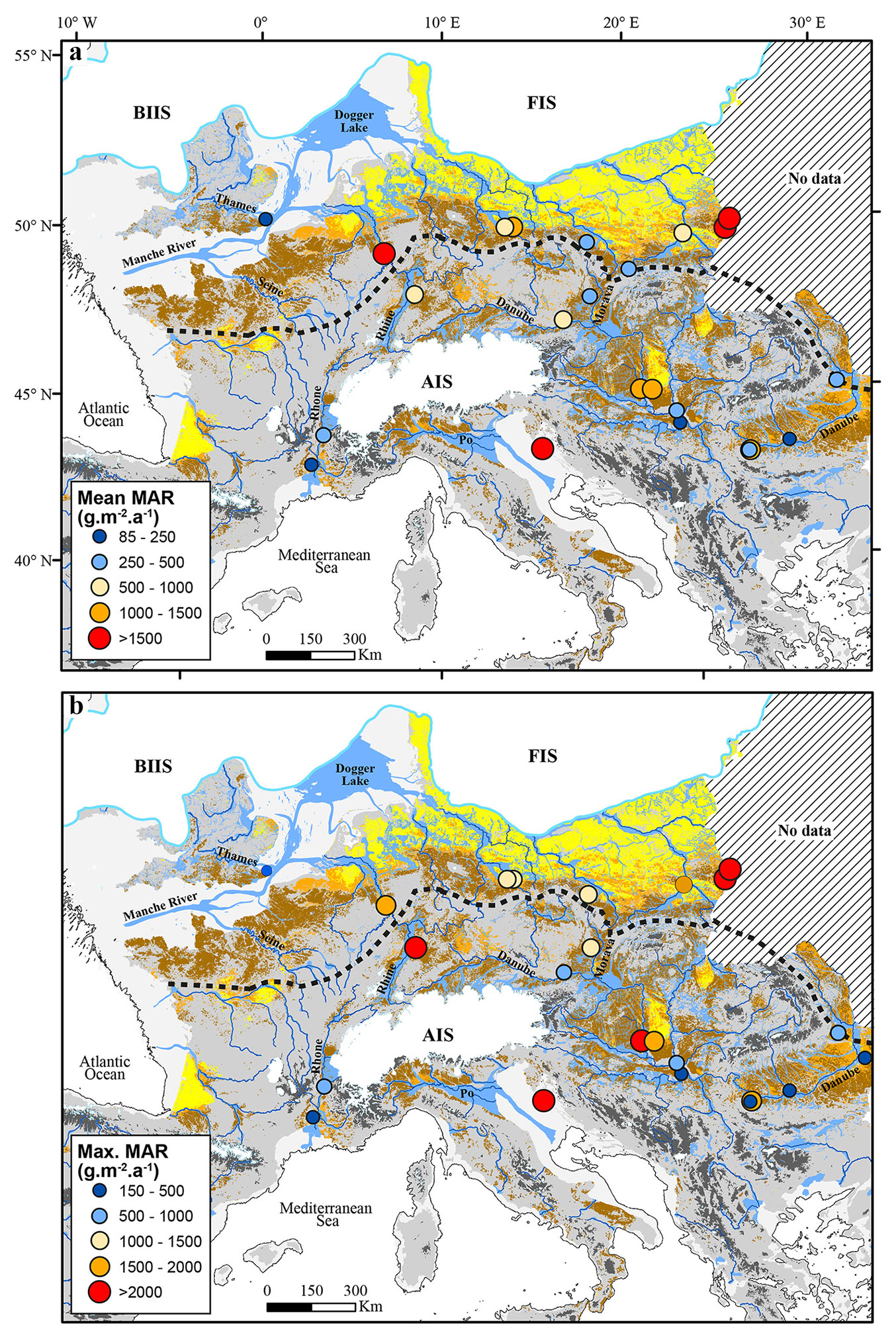
Figure 7 Mean (a) and maximum (b) MARs of European loess during the last 60 kyr b2k.

Maximum MARs are more than 3 times higher than mean MARs (Table 1). These values exceed 2000 g m⁻² a⁻¹ in eastern Poland, the Carpathian basin, the Po valley, and the Upper Rhine Graben, with a maximum of 4993 g m⁻² a⁻¹ recorded at Tyszowce (Poland) (Fig. 7). At Dunaszekcső (Hungary), our estimate of the highest MAR (3058 g m⁻² a⁻¹) agrees with that obtained by Újvári et al. (2017) using a Bayesian age–depth model performed with the Bacon software (2885 g m⁻² a⁻¹).

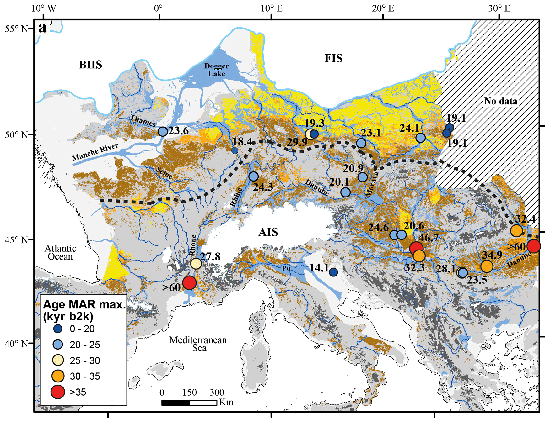
Figure 8 Age of the maximum MARs of European loess.

As most of the Last Glacial loess accumulation occurred during the time interval used to calculate average MARs, a strong correlation appears between MARs and loess thickness, as reported by, for example, Bertran et al. (2021). The thickest deposits are mainly located in the Upper Rhine Graben, the Lower Rhine Embayment, Saxony, Poland, and the Carpathian basin (middle Danube) and correspond well to areas where the highest MARs (>800 g m⁻² a⁻¹) have been recorded (Fig. 7). The Bok section located on Susak island, bordering the Po plain (Wacha et al., 2011), is also characterized by a substantial loess thickness and a high mean MAR. Several hypotheses have been put forward to explain this spatial distribution:

1. Except for Poland, the thickest loess accumulations are associated with rivers draining the AIS, suggesting that the production of glacial particles was more efficient than for the FIS and BIIS (Bertran et al., 2021). Glacial abrasion occurs under temperate and polythermal glaciers when ice slides over bedrock. The abrasion rate depends primarily on ice velocity and thickness (modulating the pressure applied to the bed) and bedrock resistance (e.g. Hallet, 1979; Iverson, 1990; de Winter et al., 2012). These factors explain Alpine glaciers' high production of fine particles due to the steep valley slopes and relatively soft bedrock, composed mainly of sedimentary rocks as opposed to the plutonic and metamorphic basements of the Scandinavian shield. For Poland, simulations by Patton et al. (2016) reconstructed high ice displacement velocities in the north of Poland (the Baltic Sea ice stream), which was favourable for glacial particle production.

2. Relief and vegetation cover played an important role in loess accumulation and probably contributed to the latitudinal differences in loess thickness. In the low-relief plains of the NELB covered by herbaceous vegetation, loess deposits form extensive blankets, whose thickness slowly decreases away from sources. In contrast, loess accumulated more locally in southern Europe but often to a great thickness near the sources due to steeper relief and taller vegetation cover, efficiently trapping the particles (Bosq et al., 2018; Bertran et al., 2021).

3. A preservation bias possibly exists related to the depositional context of perialpine and NELB loess. Extensive erosional unconformities and deeply incised valleys have been described in some loess sections from the NELB (e.g. Antoine et al., 2001; Meijs, 2002; Lehmkuhl et al., 2016; Schirmer, 2016) and interpreted as of thermokarst origin (Antoine et al., 2001; Kadereit et al., 2013) or more broadly to reworking processes in a periglacial context (Lautridou et al., 1985; Lehmkuhl et al., 2021). The formation of permafrost and repeated thermokarst processes generated large gaps in the sedimentary record and may account in part for the lower mean MARs than in more southerly regions.

Examination of the period of maximum MAR value for each LPS shows significant disparities (Fig. 8). Two areas can be distinguished: one corresponding to the NELB where ages are recent and relatively homogeneous, ranging from 29.9 to 18.4 kyr b2k, and the other to the perialpine loess that shows greater heterogeneity, with ages spread over a longer period (>60 to 14.1 kyr b2k). The combination of factors that could potentially explain this heterogeneity is the non-synchrony of glacial advances in the Alpine massif depending on the valleys (e.g. Braakhekke et al., 2020; Gribenski et al., 2021; Kamleitner et al., 2022) in agreement with simulations (Seguinot et al., 2018), and local sedimentation conditions. At the local scale, loess accumulation and erosion would have been controlled by site specificity, particularly geomorphic location, topography, local winds, vegetation, and sediment availability in river floodplains (Bokhorst et al., 2011; Stevens et al., 2011; Fenn et al., 2021). Climatic changes could thus have had a significant impact in a context of more contrasted relief than for the northern European plains.

4.3 The future potential of the ChronoLoess database

The idea of pooling luminescence data from literature and making them more accessible is not new, and efforts made in repositories such as the INQUA Dune Atlas (Lancaster et al., 2016) or OCTOPUS (Codilean et al., 2018, 2022) indicate a specific demand. Challenges remain: luminescence ages are not necessarily compatible across different studies. If used to derive broader implications, such as presented here, age values alone are insufficient, but all numerical values used for the age calculations are required to avoid systematic deviations. Since we did not have access to the original data (measured physical quantities, such as luminescence), our approach is still imperfect. However, for the first time, we attempted to extract all available data and combine them to render a bigger picture, i.e. the Last Glacial loess history in Europe.

Beyond our study, however, our data can be used for additional analyses such as for studies on the encountered environmental radioactivity.

5 Code and data availability

All open-access data described and presented in this contribution are available at Zenodo, https://doi.org/10.5281/zenodo.7728616 (Bosq et al., 2023).

6 Conclusions

The chronological study of European loess sections shows that the two major aeolian systems, the NELB on the one hand and the systems associated with the rivers draining the AIS on the other hand, did not develop synchronously. The significant deposition started at about 32 kyr b2k for the NELB versus 42 kyr b2k for the perialpine loess and peaked about 2 millennia later for the former (21.8 vs. 23.9 kyr b2k, respectively). This shift resulted mainly from the time lag between the maxima of the AIS and BIIS–FIS, which acted as the primary sources of fine-grained particles through glacial abrasion. The major geomorphic changes that resulted from the development and decay of the BIIS and FIS also played an important role. Particularly, ice sheet coalescence during the LGM diverted meltwater fluxes through the Channel River and provided huge amounts of glacial particles available for deflation in the W-NELB. The mean MAR obtained in this study from 23 LPSs reaches 792 g m⁻² a⁻¹ over the last 60 kyr b2k and falls within the range of published values, while maximum MARs reach up to 4993 g m⁻² a⁻¹. The period during which the maximum MAR is recorded for each LPS is relatively homogeneous in the NELB and ranges from 30 to 19 kyr b2k, whereas it is more scattered in the perialpine systems (>60 to 14 kyr b2k). This probably resulted from a combination of factors, including the asynchrony of maximum valley glacier advances and local geomorphic factors. The ChronoLoess database will be extended over time as new data become available.