the Creative Commons Attribution 4.0 License.
the Creative Commons Attribution 4.0 License.
 | 06 Oct 2023
An integrated and homogenized global surface solar radiation dataset and its reconstruction based on a convolutional neural network approach
Boyang Jiao
Yucheng Su
Veronica Manara
Martin Wild
Surface solar radiation (SSR) is an essential factor in the flow of surface energy, enabling accurate capturing of long-term climate change and understanding of the energy balance of Earth's atmosphere system. However, the long-term trend estimation of SSR is subject to significant uncertainties due to the temporal inhomogeneity and the uneven spatial distribution of in situ observations. This paper develops an observational integrated and homogenized global terrestrial (except for Antarctica) station SSR dataset (SSRIHstation) by integrating all available SSR observations, including the existing homogenized SSR results. The series is then interpolated in order to obtain a 5∘ × 5∘ resolution gridded dataset (SSRIHgrid). On this basis, we further reconstruct a long-term (1955–2018) global land (except for Antarctica) SSR anomaly dataset with a 5∘ × 2.5∘ resolution (SSRIH20CR) by training improved partial convolutional neural network deep-learning methods based on 20th Century Reanalysis version 3 (20CRv3). Based on this, we analysed the global land- (except for Antarctica) and regional-scale SSR trends and spatiotemporal variations. The reconstruction results reflect the distribution of SSR anomalies and have high reliability in filling and reconstructing the missing values. At the global land (except for Antarctica) scale, the decreasing trend of the SSRIH20CR (−1.276 ± 0.205 W m−2 per decade) is smaller than the trend of the SSRIHgrid (−1.776 ± 0.230 W m−2 per decade) from 1955 to 1991. The trend of the SSRIH20CR (0.697 ± 0.359 W m−2 per decade) from 1991 to 2018 is also marginally lower than that of the SSRIHgrid (0.851 ± 0.410 W m−2 per decade). At the regional scale, the difference between the SSRIH20CR and SSRIHgrid is more significant in years and areas with insufficient coverage. Asia, Africa, Europe and North America cause the global dimming of the SSRIH20CR, while Europe and North America drive the global brightening of the SSRIH20CR. Spatial sampling inadequacies have largely contributed to a bias in the long-term variation of global and regional SSR. This paper's homogenized gridded dataset and the Artificial Intelligence reconstruction gridded dataset (Jiao and Li, 2023) are both available at https://doi.org/10.6084/m9.figshare.21625079.v1.
- Article
(8401 KB) - Full-text XML
-
Supplement
(10412 KB) - BibTeX
- EndNote


Energy flows at the Earth's surface play an essential role in climate change and human activity and link to physical processes such as global warming, glacier retreating, the hydrological cycle and the carbon budget (Hoskins and Valdes, 1990; Peixoto et al., 1992; Trenberth and Fasullo, 2013; Wild, 2012). As a critical factor characterizing surface energy flows, surface solar radiation (SSR) largely determines the climatic conditions and ecological environment in which we live. Therefore, a more accurate and comprehensive analysis of the SSR fluxes will help better understand the Earth's atmospheric system. In situ observations provide the most accurate baseline data for measuring SSR. They allow for the first time the detection of decadal changes in SSR known as “dimming and brightening” (Wild et al., 2005), especially considering that they cover a longer period concerning another type of data, e.g. satellite data (Pfeifroth et al., 2018). Even observational data often have uneven distribution and missing data with respect to the satellite data, especially in areas with complex orography (Manara et al., 2020).
The sources of in situ SSR observations are mainly collected from the Global Energy Balance Archive (GEBA) (Wild et al., 2017) and the World Radiation Data Centre (WRDC) (Tsvetkov et al., 1995). Furthermore, other SSR station series are obtained from the high-quality Baseline Surface Radiation Network (BSRN) (Driemel et al., 2018) and the data centres of individual national hydrometeorological services. However, two issues still need to be addressed: (1) the inhomogeneity of station data resulting from station relocations and instrumentation changes severely impacting the climate change assessment. For the regions with a relatively high density of stations, like Europe (Manara et al., 2019, 2016; Sanchez-Lorenzo et al., 2013a, b, 2015), Japan (Ma et al., 2022) and China (Ju et al., 2006; Wang, 2014; Wang et al., 2015; Wang and Wild, 2016; S. Yang et al., 2018; You et al., 2013), much previous work has redefined the degree and timing of dimming and brightening by addressing the inhomogeneity of the SSR data series. For example, in Spain, the average annual homogenized SSR series has a significant increasing trend (+3.9 W m−2 per decade) during the 1985–2010 period (Sanchez-Lorenzo et al., 2013a). The period of dimming observed in Italy's homogenized SSR series is not apparent in the 1960s and early 1970s, when the raw series (non-homogenized) are taken into account (Manara et al., 2016). The direct measurements of SSR show a level trend from 1961 to 2014 over Japan, while their homogenization series display a decreasing trend (0.8–1.6 W m−2 per decade) (Ma et al., 2022). In China, homogenization largely eliminated the dramatic non-climatic rise of the early 1990s and also reduced the increasing trend from 1990 to 2016 (S. Yang et al., 2018). However, most of the research was still limited to regional scales. (2) There is the issue of limited spatial sampling of long observational stations and their uneven distribution, especially over areas with complex orography. Considerable efforts have been devoted to filling in or interpolating the missing values in climate datasets (“spatial analysis”) (Collins, 1996; Erxleben et al., 2002; Scudiero et al., 2016). The traditional spatial interpolation methods commonly used include inverse distance weighting (Fisher et al., 1993; Shepard, 1968), kriging (Krige, 1951) and thin-plate splines (Bookstein, 1989). Since the 1980s, physical parametric interpolation (Feng and Wang, 2021; Tang et al., 2019) and Bayesian fusion schemes (Aguiar et al., 2015) based on multi-source observational data have been widely used with the emergence of highly accurate and relatively precise satellite data. However, the resulting fusion datasets cover too short a period to investigate their decadal and multi-decadal variations and to study the underlying causes. The spatial, temporal and spectral coverage of a single satellite is limited, and multiple satellite data are therefore often used in tandem with each other; however, such a discontinuity in time and space can introduce inhomogeneity into a dataset (Evan et al., 2007; Feng and Wang, 2021; Shao et al., 2022). Reanalysis products are an important complement containing long-term SSR data and therefore have been widely used in climate studies (Huang et al., 2018; Jiao et al., 2022; Urraca et al., 2018; C. Zhou et al., 2018, 2017) due to the dynamically consistent and spatiotemporally complete atmospheric fields with high resolution and open access to data. However, existing studies have shown that reanalysis products generally overestimate multi-year mean SSR values compared to observations over land (He et al., 2021). With the continuous development of climate system simulations, model data from the Coupled Model International Project (CMIP) have become an important resource for conducting climate change research (Gates et al., 1999; Zhou et al., 2019). Previous studies have shown that the models used in CMIP6 overestimate the global mean SSR (He et al., 2023; Jiao et al., 2022; Wild, 2020). The rise of deep-learning and big-data techniques has brought about an explosion of artificial intelligence (AI). Machine learning is increasingly being used in spatial interpolation, such as the spatial reconstruction of surface temperature datasets (Huang et al., 2022; Kadow et al., 2020) or the spatial and temporal reconstruction of turbulence resolution (Fukami et al., 2021). Furthermore, it shows high accuracy and low uncertainty in reproducing and predicting SSR (Leirvik and Yuan, 2021; Tang et al., 2016; L. Yang et al., 2018; Yuan et al., 2021). However, long-term homogenized SSR datasets with global terrestrial coverage have yet to be developed, resulting in significant uncertainties in assessing global SSR variation (Jiao et al., 2022).
Therefore, developing a more homogeneous and comprehensive global long-term SSR climatic dataset that provides a better benchmark for observational constraints on the global surface energy balance and budget remains a valuable and challenging task. This paper first homogenizes and grids the most extensive collection of available global SSR station observations. Then, the missing grid boxes and years are spatially interpolated using a convolutional neural network (CNN) approach to obtain a globally covered land surface SSR anomaly dataset. Finally, the reconstructed datasets are initially analysed and evaluated. Thus, the paper is divided into seven main sections. The data resources are introduced in Sect. 2. Section 3 presents the data homogenization and the CNN model reconstruction methods. The data homogenization and verification are shown in Sect. 4. Section 5 gives the AI reconstruction results. Section 6 is the availability of the datasets. Conclusions are provided at the end of the paper.
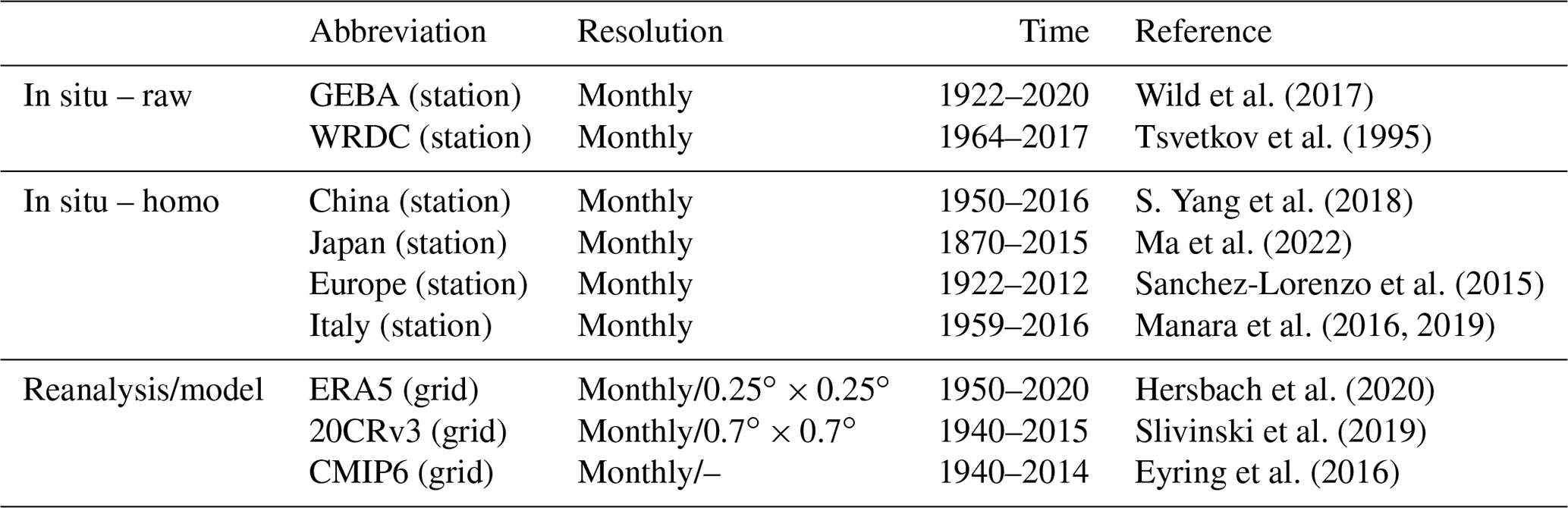
Nine SSR datasets are collected to derive the global SSR variable. In particular, six datasets contain data from observational stations (Sect. 2.1): two global ground-based measurement datasets (GEBA, WRDC) and four homogenized products at the regional and country levels (Europe, China, Japan and Italy). Three of the adopted datasets are reanalysis data (Sect. 2.2.1): fifth-generation European Centre for Medium-Range Weather Forecasts (ECMWF) reanalysis (ERA5), 20th Century Reanalysis version 3 (20CRv3) data and the Coupled Model Intercomparison Project Phase 6 (CMIP6) historical simulation output (125). Specifically, the ERA5 data are used to fill the data over oceans and Antarctica (Sect. 3.2.1), and 20CRv3 data and CMIP6 simulations are used for AI model training (Sect. 5.1) and reconstruction. All are listed in Table 1.
Table 1List of information on the various types of data used in this paper.
2.1 In situ observational data
2.1.1 Global datasets
There are two main sources of raw SSR data (see Table 1): the ETH Zurich GEBA with monthly data from 2445 globally distributed stations, starting from 1922 until 2020, and the WRDC dataset with monthly globally distributed data from 1136 stations since 1964. The first one is available for download at https://geba.ethz.ch (last access: 2 July 2022). The second one published the first SSR radiation balance data in 1965, and its publication has been issued four times a year since 1993 and is available for download at http://wrdc.mgo.rssi.ru/ (last access: July 2021).
2.1.2 National (regional) homogenized station datasets
(1) Chinese homogenized SSR dataset
The China Meteorological Radiation Fundamental Elements Monthly Value Data Set was downloaded from http://www.nmic.cn (last access: September 2022). The homogenized SSR dataset in China is released by the National Meteorological Information Centre (NMIC) of the China Meteorological Administration (CMA) (S. Yang et a., 2018). The data are available for the period between January 1950 and December 2014, and the follow-up data are extended with raw observations from the NMIC. They used the sunshine duration (SSD) data from nearby stations to construct an arguably better reference to identify inhomogeneities in the SSR data. Then, a combined metadata and maximum-penalty t-test (PMT) method was used to detect the change points. Finally, they were adjusted by a quantile-matching (QM) algorithm (Wang and Feng, 2013). The final homogenized SSR station dataset was converted to gridded data using the first difference method (FDM, Peterson et al., 1998) and is available for download at http://www.nmic.cn (last access: September 2022).
(2) Japanese homogenized SSR dataset
Ma et al. (2022) released a Japanese SSR homogenized dataset in 2022 spanning the period between 1870 and 2015. First, they homogenized SSD based on PMF (penalized maximal F test) and QM algorithms. They then used the homogenized SSD from the previous step as a reference series, combined with metadata and PMT, to detect change points. Finally, they adjusted the change points by the QM algorithm. For more details on data descriptions, the adopted methodology and downloading data, see https://data.tpdc.ac.cn/en/data/45d73756-3f5a-4d27-82a4-952e268c20e8/ (last access: March 2022).
(3) European homogenized SSR data
A homogenized dataset of European SSR stations was developed by Sanchez-Lorenzo et al. (2015) and is currently available for full public download at https://doi.org/10.1002/2015JD023321. They selected the 56 longest central European SSR series available in the GEBA dataset with data for the period between 1922 and 2012. They adjusted them to ensure temporal homogeneity, homogenizing the data with the standard normal homogeneity test (Alexandersson, 1986) and the Craddock test (Craddock, 1979).
(4) Italian homogenized SSR dataset
The Italian homogenized SSR datasets are those published by Manara et al. (2019, 2016). As candidate stations to use as reference series, they selected the 10 series located in the same area of the series to be tested, and that series correlates well with the test one. In particular, they tested the change points with the Craddock test (Manara et al., 2017), and when a break is identified by more than one reference series, the preceding portion of the series is corrected, leaving the most recent portion unchanged. In this way, the SSR stations were homogenized, and then the missing values were interpolated.
2.2 Other datasets
2.2.1 Reanalysis
ERA5 can be used to fill in SSR data from the oceans and Antarctica and carry out the global reconstruction, taking into account its high spatial resolution and the reliable performance of SSR (Jiao et al., 2022; Liang et al., 2022). After the reconstruction, we removed the data for the ocean reanalysis and maintained the data only in the land area (except for Antarctica). In addition, two SSR data products (20CRv3, CMIP6) are used to train AI models. These are the following.
-
ERA5 (space-filling data). ERA5 is the fifth generation of the European Centre for Medium-Range Forecasts reanalysis product, which currently publishes data from 1950 to the present (Hersbach et al., 2020). In addition, ERA5 has an hourly output and an uncertainty estimate from the ensemble. The data are based on the Integrated Forecasting Model Cy41r2 run in 2016, which contains a 4D-Var assimilation scheme. In ERA5, SSR is obtained from a rapid radiation transfer model (RRTM) (Mlawer et al., 1997). The present study utilizes monthly SSR data for the period 1955–2018 from ERA5 with a resolution of 0.25∘ × 0.25∘. They can be downloaded at https://cds.climate.copernicus.eu (last access: July 2022).
-
20CRv3 (data for AI model training). The 20CR project is an effort led by the NOAA's Physical Sciences Laboratory and CIRES at the University of Colorado, supported by the Department of Energy, to produce reanalysis datasets spanning the entire 20th century and much of the 19th century (Slivinski et al., 2019). 20CR provides a comprehensive global atmospheric circulation dataset from 1850 to 2015. Its chief motivation is to provide an observational validation dataset, with quantified uncertainties, for assessing climate model simulations of the 20th century. 20CR uses an ensemble filter data assimilation method which directly estimates the most likely state of the global atmosphere every 3 h and estimates the uncertainty in that analysis. The most recent version of this reanalysis, 20CRv3, provides 8-times daily estimates of global tropospheric variability across 75 km grids, spanning 1836 to 2015 (with an experimental extension from 1806 to 1835). The present study uses monthly SSR data of 20CRv3 (NOAA/CIRES/DOE 20CR, 80 members) from 1955 to 2015. We selected all 80 members of the 20CR as input (1 for evaluation and to test reconstruction, the other 79 for training the CNN model). The SSR of 20CRv3 has a spatial resolution of 0.7∘ × 0.7∘. The download is available at https://portal.nersc.gov/archive/home/projects/incite11/ (last access: May 2022).
2.2.2 CMIP6 model output
- 3.
CMIP6 model output (data for AI model training). The Coupled Model Intercomparison Project, driven by the World Climate Research Program, is now in its sixth phase. Specifically, CMIP6 is considered the current state-of-the-art way of producing future climate simulations, including predicting future SSR based on different climate scenarios (W. Zhou et al., 2018). It provides an important resource for studying current and future climate change (Eyring et al., 2016). The historical simulations of CMIP6 are designed to reproduce observed climate and climate change constrained by radiative forcing. CMIP6 historical simulation spans between 1850 and 2014. In this study, we selected 125 members out of a total of 507 members from several CMIP6 large-ensemble models (with more than 10 realizations and runs) with high correlation coefficients with observations as input to train and validate the CNN model (1 for evaluation and to test reconstruction, the other 124 for training the CNN model). We selected the monthly downward shortwave radiation from 1955 to 2014 (see Table S1 in the Supplement). The data can be downloaded at https://esgf-node.llnl.gov/search/cmip6 (last access: July 2022).
3.1 Data quality control (QC) and homogenization
The SSR data homogenization method is only applied to the two non-homogenized in situ observation datasets (GEBA and WRDC). The QC and homogenization flowchart (Fig. 1) is divided into three steps: (1) QC; (2) homogenization; and (3) integration and consolidation.
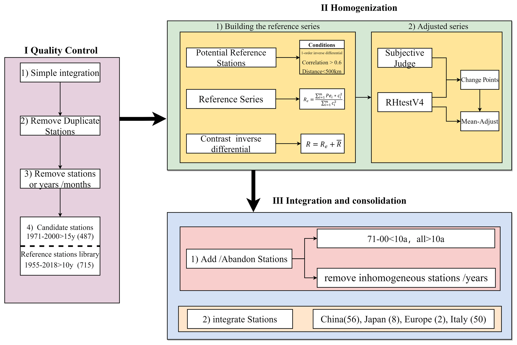
Figure 1Flowchart of quality control (QC) (first step), homogenization (second step) and integration (third step).
3.1.1 QC
The QC of SSR data includes the following steps.
-
Simple integration is integration of the GEBA (2445) and WRDC (1136) datasets, removing stations with no data and leaving 2681 stations.
-
Removing duplicate stations. (a) For stations with similar latitude and longitude, we consider two stations with totally identical latitude and longitude to be the same station. (b) For stations less than 10 km apart, we averaged the duplicate stations in these a and b cases. (c) For special duplicate stations, we stitched together data of the duplicate stations based on metadata from the CMA.
-
Remove stations, years or months for which a climatic analysis cannot be established: we remove stations with records of less than 10 years and values more than 3 times (3σ criterion, Olanow and Koller, 1998) the standard deviation of the SSR anomalies.
-
Candidate stations (487) with a record length greater than 15 years in the period 1971–2000 are selected. We added stations (715) with more than 10 years of SSR records to increase the number of available stations for a better homogenization of the candidate stations (Fig. 2).
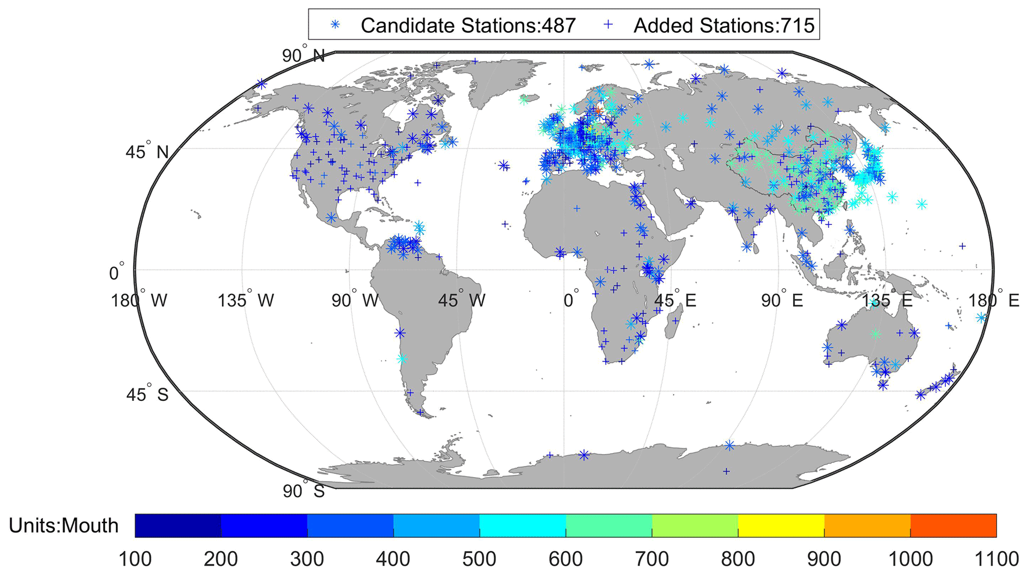
Figure 2Spatial distribution of candidate stations (“*”) and added stations (“+”). The different colour bars represent the length of the station record in months.
3.1.2 Station series homogenization
This paper uses the RHtestV4 software package to test and adjust the SSR station data for homogeneity (http://etccdi.pacificclimate.org/software.shtmlm last access: July 2021) (Wang and Feng, 2013). The package is based on the empirical penalty functions PMF (Wang, 2008a) and PMT (Wang, 2008b; Wang et al., 2007) for the homogenization test. It takes into account the lag-1 autocorrelation of the time series. It embeds a multiple linear regression algorithm to significantly reduce the problem of an unbalanced distribution of pseudo-identification rates and test efficacy. Also, RHtestV4 uses the QM algorithm (Vincent et al., 2012; Wang et al., 2010) and mean adjustments to adjust the identified change points.
The specific steps are as follows.
- 1.
Building the reference series
- a.
We processed the data from all station series (715) into the annual first difference (FD) series ei (Eq. 1) (Peterson et al., 1998).
- b.
We calculated the correlation of the annual FD series between the series from the potential reference pool and the candidate stations.
- c.
We calculated the distance between the potential reference pool stations and candidate stations.
- d.
We selected potential stations according to the correlation coefficient (CC > = 0.6) between the series from potential reference pool and candidate stations. The potential stations also satisfy the limits in distances (< = 500 km) between the potential pool stations and candidate stations.
- e.
We obtain the reference FD series (Re) based on the m potential reference series (Pei) and the CCs (ci) between the potential reference series (Pei) and candidate station series (Eq. 2).
- f.
The synthesized reference FD series (Re) (Eq. 2), plus the average of all potential reference series (), yields the final annual reference series (R) (Eq. 3).
xi is the raw observational station SSR in the year i, Re is the final reference series, Pei is the potential reference series, and ci is the CC between the potential reference series and the candidate station series.
- a.
- 2.
Testing and adjusting the candidate series
The homogenization test algorithm used in this paper is the PMT. This method is a reference series-dependent test for a normalized candidate series. It assumes that the linear trend of the time series is zero and uses the degree of mean deviation at different points in the series to find change points. Furthermore, it eliminates the effect of different sample lengths on the test results. At the same time, the method introduces an empirical penalty factor, which effectively improves detection. We used the PMT to test the homogeneity of the candidate series based on the reference series established in (1). We then adjusted the statistically significant (p>0.05) change points obtained using the mean adjustment method (p>0.05). We homogenized the monthly series for 66 stations (see Fig. S1 in the Supplement).
3.1.3 Integration and consolidation
As can be seen from Fig. 1, the candidate stations (487) are relatively sparse. To better adapt deep-learning methods for the dataset reconstruction later, we adjusted, added and integrated station series based on the results of homogenized data from other scholars. (1) We added stations with more than 10-year overall (1955–2018) records but no more than 15 years during the 1971–2000 period and removed those stations that were clearly inhomogeneous (25) and some years of station (3). (2) We subsequently integrated monthly SSR series for 116 stations based on the results of homogenization from other scholars: China (56), Japan (8), Europe (2) and Italy (50). After the above steps, we ended up with a homogenized dataset containing 944 stations (Fig. 3). The details of the processing and classification are shown in Table S2 (see the Supplement).
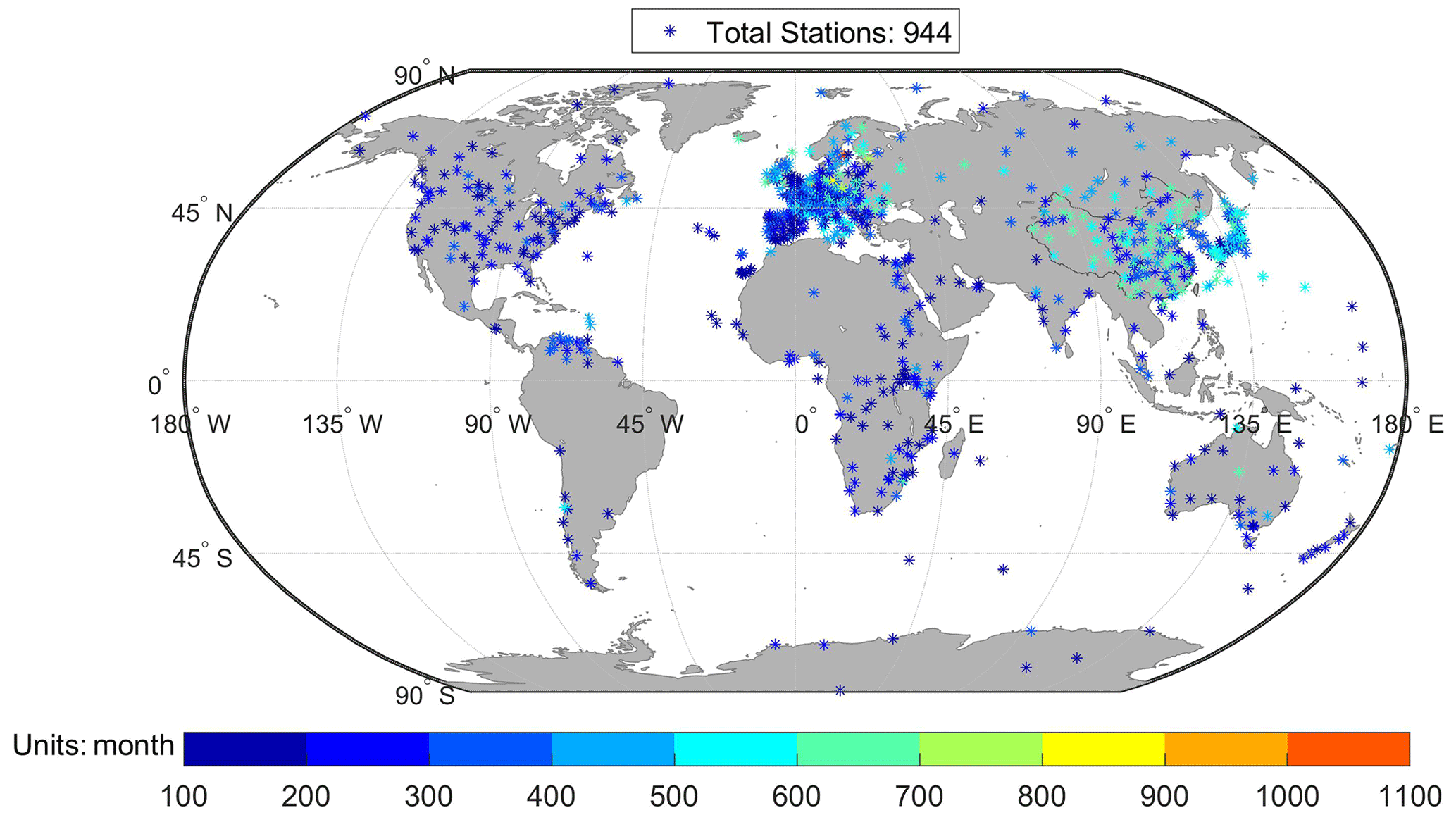
Figure 3Spatial distribution of stations after homogenization (unit months). Different colours represent the length of the station records in months.
3.2 CNN model reconstruction methods
The CNN deep-learning model network architecture uses a U-shaped structure similar to U-Net (Ronneberger et al., 2015). The advantage of using this model is that (1) both high- and low-frequency information of the picture can be retained, and when reconstructing the SSR data, not only will the grid point information close to the missing measurement point be considered, but information from more distant locations will be too (which may be remotely correlated with that missing measurement point). (2) This makes the model convergence faster and more economical in terms of computational resources. The upper part of the U-shaped structure, which has no downsamples or a low number of downsamples, represents the high-frequency information of the graph. These sections contain much of the detail in the graph, and the relationships between similar grid points are conveyed by this section. The lower half of the U-shaped structure is downsampled more often and represents the lower-frequency information of the graph. The global radiation of a wide range of undulations is transmitted by it, and then the information at the various levels of the U-shaped structure is connected and transmitted through the skip connection, allowing the whole network to remember all the information of the picture very well. The model uses nearest-neighbour upsampling in the decoding phase, and the skip links will concatenate two feature maps and two masks as the feature and mask inputs for the next part of the convolution layer. The input to the last part of the convolution layer will contain the original input image concatenated with the holes and the original mask, allowing the model to replicate the gap-free pixels. The complex and variable nature of the sea–land boundary then has a significant impact on the reconstruction when we reconstruct the global land SSR data. Therefore, we use partial convolution at the image boundaries with a suitable image padding, ensuring that the padding content at the image boundaries is not affected by values outside the image. The deep-learning models' convolutional layers and loss functions are described in the Supplement.
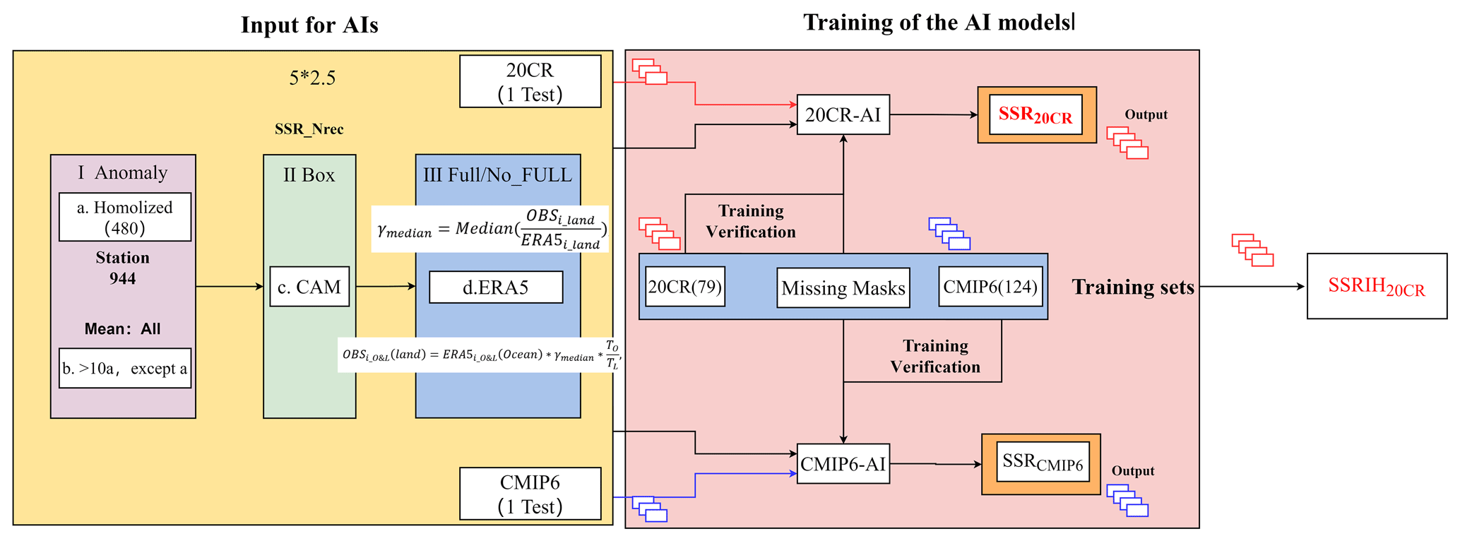
We further reconstruct a long-term (1955–2018) global SSR anomaly dataset (SSRIH20CR) by using improved partial CNN deep-learning methods based on a “perfect” dataset. A CNN consists of three parts: a convolutional layer to reduce the number of weights by extracting local features, a pooling layer to reduce peacekeeping and prevent overfitting, and a fully connected layer to output the desired result. In this paper, a modified CNN is used to model the reconstruction of the SSR data, with the convolutional layer replaced by a partial convolution method and mask update. This method is the latest in image restoration effects and can restore irregular holes, an advantage over other image restoration methods that can only restore rectangular holes. Therefore, this paper uses the modified CNN model (Kadow et al., 2020) to recover the missing part of the global terrestrial SSR (except Antarctica). The specific reconstruction steps and processes are as in Fig. 4.
3.2.1 Data pre-processing
The homogenized station data are converted to grid box anomalies using the climate anomalies method (CAM) (Jones et al., 2001). CAM is a commonly used method for converting station anomaly data to gridded data. We divide all global areas into a 5∘ × 5∘ grid, after which we calculate the SSR anomalies (relative to 1923–2020) within the grid box by averaging the anomalies of all the stations (at least one station in it). If more than one site exists in the same grid box, the record length of this grid box is the total length of all sites in that grid box. Finally, we removed the values that were more than 3 times the standard deviation of the SSR anomaly time series after gridding. SSRs are all processed as daily average anomalies, i.e. monthly anomalies divided by 30 (each month is approximated as 30 d). We multiply all the values by 30 again when the reconstruction is complete. The global land (except for Antarctica) distribution and coverage of SSRs after gridding are shown in Fig. 5a, b.
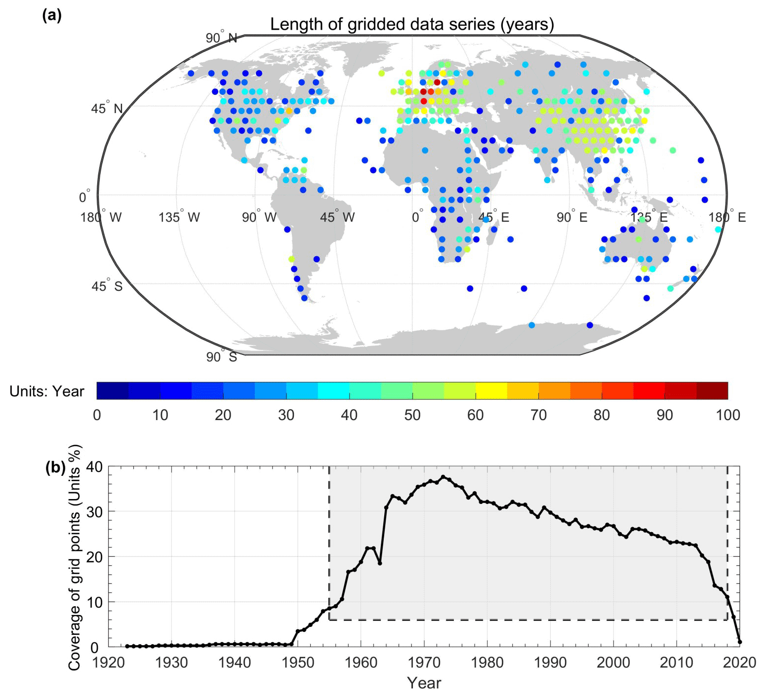
Figure 5(a) Spatial distribution of 5∘ × 5∘ grid boxes (SSRIHgrid) obtained by interpolating the homogenized global land (except for Antarctica) SSR series. The different colours represent the length (the sum of all the records) of the station record in unit years. (b) Grid box coverage for the homogenized global land (except for Antarctica) SSR (SSRIHgrid) except for Antarctica.
As seen in Fig. 5a, the SSR is spatially sparsely distributed across South America and Africa. As shown in Fig. 5b, SSR coverage increased yearly from 1950 until the mid-1970s, when it slowly decreased. In 2013, the coverage rate decreased sharply due to untimely data submission. Considering the SSR coverage above, we only kept the years (1955–2018) with data coverage of more than 8 % of global land (except for Antarctica) areas.
Comparisons show that ERA5 has a high spatial resolution and relatively reliable performance in the temporal variations and long-term trends (Liang et al., 2022; Jiao et al., 2022). To obtain a higher data coverage and ensure that the AI model runs well, we used the ERA5 to fill the SSR of the homogenized global gridded SSR in the Antarctic and ocean areas. However, if we use the SSR of ERA5 to directly fill the SSR of the homogenized global gridded SSR (SSRIHgrid) in the Antarctic and in the ocean areas, then the relatively weaker ocean SSR variations (variabilities, decadal changes, trends) from ERA5 will inevitably introduce certain systematic biases in land SSR reconstruction due to the SSRs having the lower coverage on the land. Therefore, we designed an algorithm to avoid excessive diffusion of SSR system bias in terrestrial areas: we first calculated the ratios between the SSR from ERA5 and from SSRIHgrid on the land in all n years. For a single grid box, the γi have small changes and are regarded as a constant γmedian (Eq. 4), and the γmedian vary by latitude and longitude in both the marine and land areas. We then extrapolated the γmedian for all the grid boxes along the land and sea boundaries. If there is no observation there, then the adjacent ocean ERA5 SSR is used to take its place after it is adjusted according to the differences between the SSR variations (represented by the linear trends) for the different underlying surfaces (Eq. 5):
γmedian is the median value of the ratios of observation (OBS) and ERA5 land SSR series. OBSi_land is the land SSR for the year i from the SSRIHgrid in a single grid. ERA5i_land is the land SSR for the year i from ERA5 in a single grid. OBSi_O&L(land) is the land SSR along the sea–land boundary (land) for the year i from the SSRIHgrid. ERA5i_O&L(ocean) is the ocean SSR along the sea–land boundary for the year i from ERA5. TO is the trend of the ERA5 SSR in ocean areas in all n years, and TL is the trend of the ERA5 SSR in areas in all n years.
3.2.2 AI model reconstruction
We use a server (configured with processor Intel (R) Core (TM) i7-8700 CPU @ 3.20 GHz 3.19 GHz, RAM 32G, 64-bit OS, GPU model 516.94, NVIDIA GeForce 1080T version, Python 3.9.12 64-bit, CUDA 10.1) for AI model training. The specific training steps are as follows.
-
A total of 768 missing-value masks (monthly masks between 1955 and 2018) were prepared for training and validation using “1” for existing and “0” for missing values.
-
The 20CRv3–CMIP6 training set (monthly values between 1955 and 2015/2014) and missing-value masks are fed into the 20CR-AI and CMIP6-AI model for training.
-
We perform 1 500 000 training sessions with an interval of 10 000 sessions for the training output model.
Afterwards, the two AI models are validated against the root mean squared error (RMSE) and CCs of the reconstructed SSRs (SSRSSRCMIP6). The validation set SSRs, and the optimal number of training cycles is 1 100 000 (see Figs. S2, S3 and S4 in the Supplement). The initial hyperparameters of the model are set as follows: a learning rate of and learning fine-tuning of . First, we set the batch size to 16 in the first 500 000 iterations and fine-tune it to 18 in the last 10 000 000 iterations, for a total of 1 500 000 iterations, to suppress the overfitting phenomenon generated during the training process. We validate the model every 10 000 times and with early stopping if the validation shows a decreasing trend, and the final number of training times used is 1 100 000. Second, L2 (ridge regression) regularization is also added to regulate the loss function (see Eq. S9 in the Supplement).
The training result models generated by the different AI models are obtained separately for the different training sets. The model is first used to reconstruct a reanalysis validation set with the same missing-value mask as the original observation dataset. This is followed by a validation of the reconstruction against the original reanalysis dataset (calculation of CC and RMSE) to understand the discrepancies in the model reconstruction.
We homogenized the original monthly station or gridded SSR time series (SSRIHstation or SSRIHgrid) using the method in Sect. 3.1.2. We selected six continental regions, excluding Antarctica and the Arctic, from the eight continents of the world defined by Xu et al. (2018) (Asia, Africa, South America, Europe, North America, Australia, Antarctica and the Arctic). The decreasing trend of the SSRIHgrid is consistent with the original gridded SSR series (SSRIgrid) during 1955–1991, while the increasing trend during 1991–2018 is weaker. At the regional scale, the SSRIHgrid has a generally similar variation to the SSRIgrid, and the SSRIHgrid is usually more representative of climate change than the SSRIgrid at individual stations.
Figure S5 (see the Supplement) illustrates the long-term variations of global (Fig. S5a in the Supplement) and continental land SSR (Fig. S5b in the Supplement) from the SSRIgrid and SSRIHgrid (except for Antarctica) during 1955–2018. The most prominent change revolves around the adjustment around 1992: the SSR anomalies were systematically adjusted upward from 1987 to 1992, while the SSR anomalies were systematically adjusted downward from 1993 onwards. Thus, there is a significant decreasing trend for both the global land SSRIgrid (−1.995 ± 0.251 W m−2 per decade) and global land SSRIHgrid (−1.776 ± 0.230 W m−2 per decade) (except for Antarctica) from 1955 to 1991, while the increasing trend of the global land SSRIHgrid from 1991 to 2018 is 0.851 ± 0.410 W m−2 per decade, slightly smaller than the increasing trend of the SSRIgrid (0.999 ± 0.504 W m−2 per decade). It is worth noting that 1992 happened to be the second year of the eruption of Mount Pinatubo, and the homogenized SSR data integrated in this paper may be affected by this event. However, overall, the homogenization also has limited effects on the global SSR variations from Fig. S5 (see the Supplement), which is consistent with the influence of data homogenization on a wide range of surface air temperatures (Brohan et al., 2006; Xu et al., 2013).
On the regional scale, the differences between the SSRIHgrid and SSRIgrid are more pronounced in Asia and Europe (see Fig. S5b in the Supplement). Asia's homogenized SSR shows that the regional average SSR has been declining significantly over the period 1958–1990; this dimming trend mostly diminished over the period 1991–2005 and was replaced by a brightening trend in the recent decade. The SSRIHgrid in Asia is higher than the SSRIgrid from 1985 to 1990 and lower than the SSRIgrid from 2012 to 2015. The SSRIHgrid shows a more moderate short-term increase in Europe from 1960 to 1980. Note also that the Australian raw data prior to 1988 were artificially detrended because at the time the Australia Weather Service was afraid that the instruments would drift. Therefore, they detrended them and unfortunately did not store the raw data, and the SSR evolution in Australia is artificial with no trend (Wild et al., 2005). In addition, the SSRIstation and SSRIHstation comparisons for all 66 stations are shown in Fig. S1 (see the Supplement).
5.1 Training of the AI model
We produce two (20CRv3 and CMIP6) separate training and validation sets: we select the first member data of the reanalysis data and the model data, respectively, as the validation set, and the remaining 79 (124) ensemble members as the training sets, where each ensemble member included 732 (720) months of SSR data. Each validation set included 732 (720) samples, while the training sets contained 57 828 (89 280) ensemble members. All the above data, including the in situ observations, are then resampled to monthly anomalies of 5∘ × 2.5∘. We reconstruct the SSR of 20CRv3 and CMIP6 with missing values based on the 20CRv3 and CMIP6 datasets using the method in Sect. 3.2 and obtain two reconstructions, SSR20CR and SSRCMIP6, respectively. The SSR of 20CRv3 and CMIP6 with missing values uses the SSRIHgrid mask between 1955 and 2015/2014. We compare the global land (except for Antarctica) or regional annual anomaly variation of SSR20CR or SSRCMIP6. The results show that SSR20CR is significantly more consistent with the validation set than SSRCMIP6.
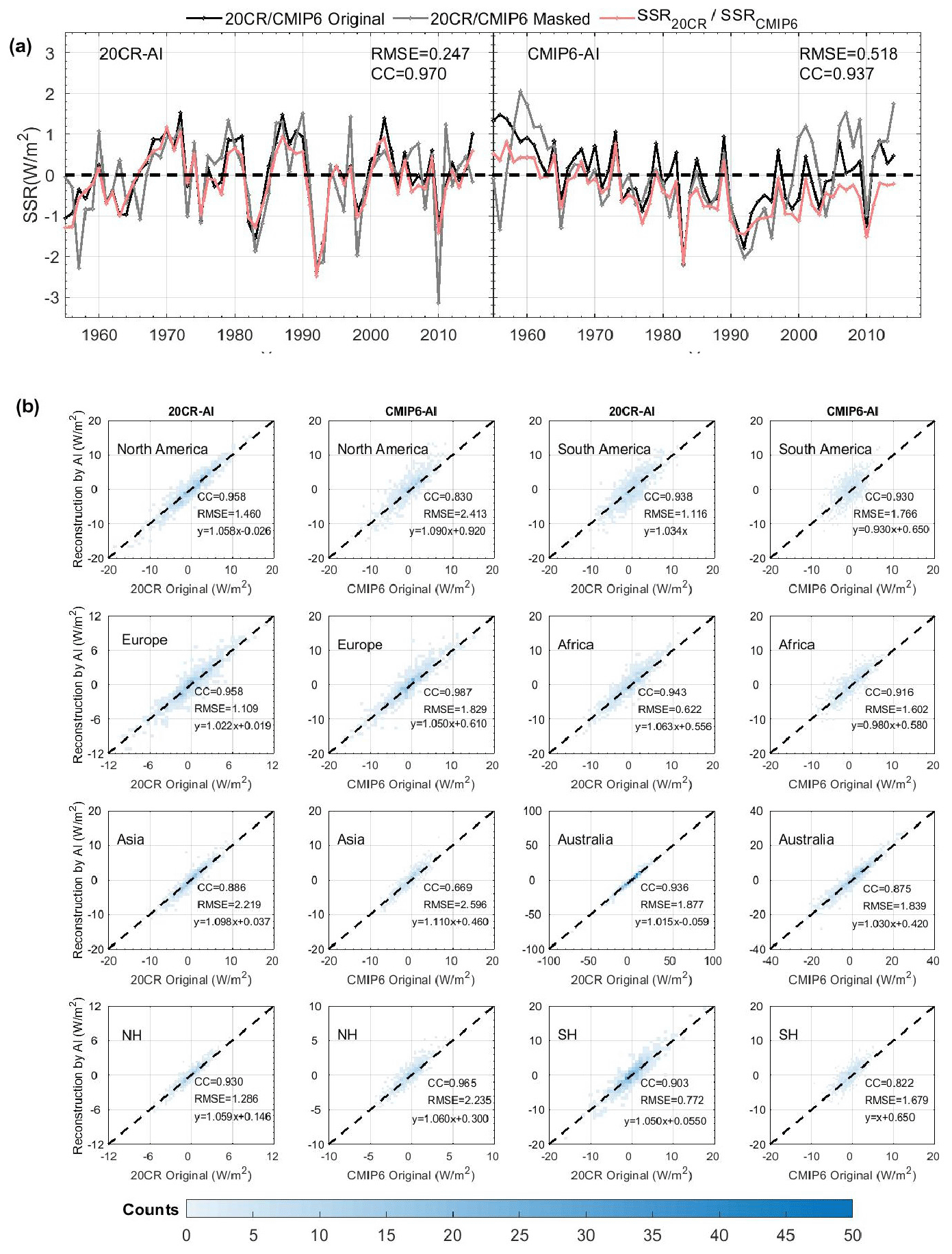
Figure 6a shows that the RMSE and CC of the SSR20CR (0.247 W m0.970 W m−2) are smaller or larger than those of the SSRCMIP6 (0.518 W m0.937 W m−2) with the original 20CR and CMIP6 dataset. The 20CR-AI model has a better reconstruction ability for SSR on the global land (except for Antarctica) scale. The RMSEs of the SSR20CR (SSRCMIP6) are 1.460 (2.413) W m−2, 1.109 (1.829) W m−2, 2.219 (2.596) W m−2 and 1.286 (2.235) W m−2 in North America, Europe, Asia and the Northern Hemisphere, whereas these values are 1.116 (1.766) W m−2, 0.622 (1.602) W m−2, 1.877 (1.839) W m−2 and 0.772 (1.679) W m−2 in South America, Africa, Australia and the Southern Hemisphere, respectively, concerning the original 20CR and CMIP6 dataset. In other words, the RMSEs of the SSR20CR are smaller than those of the SSRCMIP6 for the original 20CR and CMIP6 dataset except for Australia. In addition, the CCs of the SSR20CR (SSRCMIP6) are 0.958 (0.830) W m−2, 0.958 (0.987) W m−2, 0.886 (0.669) W m−2, 0.930 (0.965) W m−2, 0.938 (0.930) W m−2, 0.943 (0.916) W m−2, 0.936 (0.875) W m−2 and 0.903 (0.822) W m−2 in North America, Europe, Asia, the Northern Hemisphere, South America, Africa, Australia and the Southern Hemisphere, respectively, with respect to the original 20CR and CMIP6 dataset. That is, the CCs of the SSR20CR are larger than those of the SSRCMIP6 with the original 20CR and CMIP6 dataset except for Europe.
Based on the above comparison, the higher uncertainty for CMIP6 model output possibly biases the CMIP6-AI method. Thus, the accuracy of the SSR20CR is higher than that of the SSRCMIP6 at both global land (except for Antarctica) and regional scales. Therefore, we choose the reconstruction results of the 20CR-AI model as the final AI reconstruction dataset, and subsequent analysis in the following sections is only based on this dataset.
5.2 Comparison of the spatial and temporal variation characteristics
We investigate the long-term trends and spatial and temporal variation of the SSRIH20CR, compare the differences between the SSRIH20CR and SSRIHgrid, and suggest that the area and magnitude of the high and low centres of the SSRIH20CR are the same as those of the SSRIHgrid. The results of the global land (except for Antarctica) reconstruction are consistent with dimming and brightening; the global dimming is primarily dominated by decreasing trends in Asia, Europe, Africa and North America, whereas Europe and North America are contributors to the increasing trends.
Figure 7 shows the spatial distribution of the SSRIHgrid and SSRIH20CR for the 3 months (July 1960, July 1980 and July 2000). Figure S6 (see the Supplement) displays the spatial distribution of the annual SSRIHgrid and SSRIH20CR from 1955 to 2018. Figure 7 also shows that the area and the magnitude of the high and low centres in the SSRIH20CR are the same as in the SSRIHgrid. The SSRIH20CR has mainly positive anomalies in Africa and the Eurasian continent in July 1960, especially in India and the Middle East. Afterwards, India showed a continuous and steady decline in SSR. This confirms the well-known phenomenon of global dimming over India (Wild et al., 2009; Soni et al., 2016, 2012; Padma Kumari et al., 2007; Kambezidis et al., 2012). In Australia, the SSRIH20CR is dominated by negative anomalies in July 1980 and positive anomalies in July 1960 and July 2000. In Greenland, the SSRIH20CR shows a large positive anomaly during 3 months. In northern Russia, there is a high value in July 2000. The reconstruction can better reflect the anomaly distribution of observation information, and the grid boxes with the missing values are infilled and reconstructed, which has high reliability.
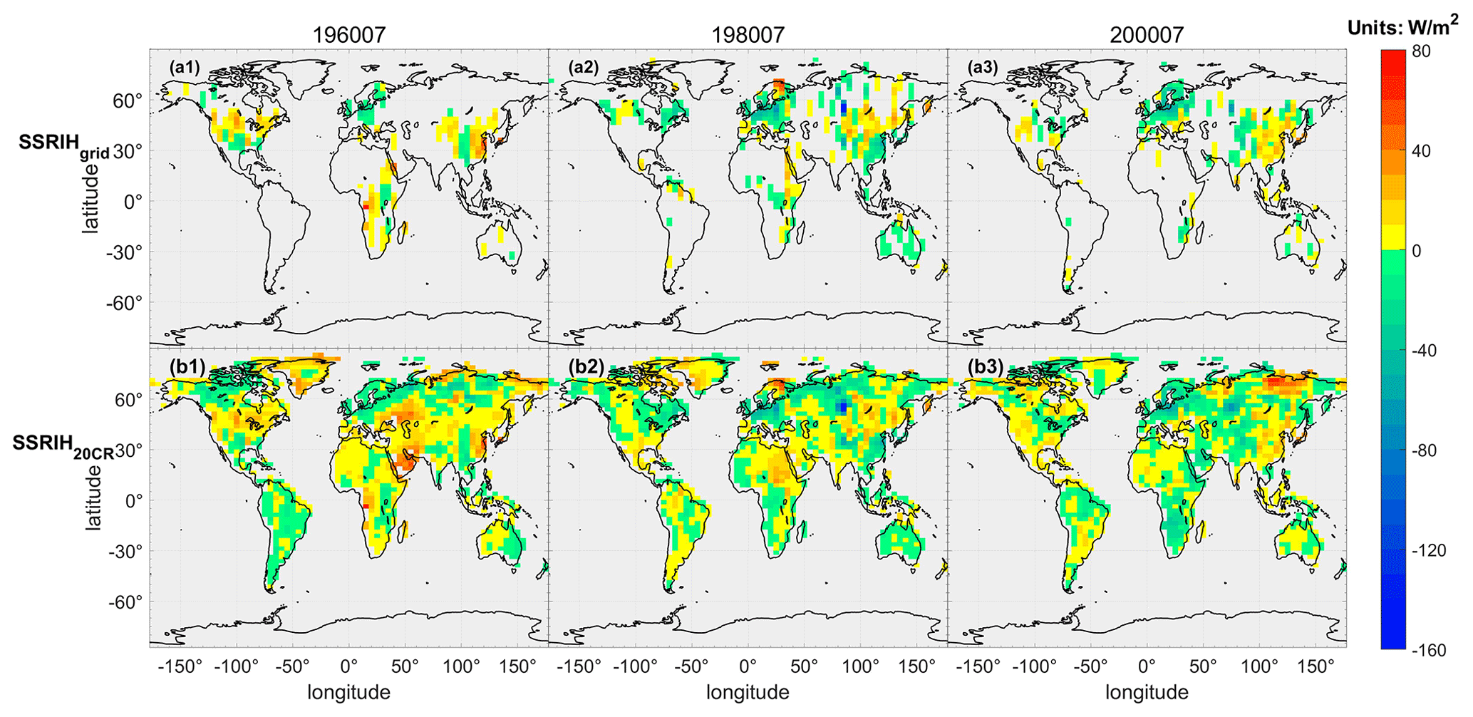
Figure 7Spatial distribution of the SSRIHgrid (a1–3) and SSRIH20CR (b1–3) in typical months: 1–3 are July 1960, July 1980, and July 2000, respectively.
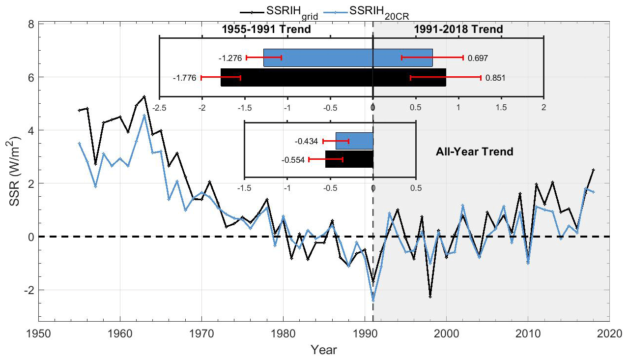
Figure 8Global land (except for Antarctica) time series of the annual anomaly variations' SSR (relative to 1971–2000) before and after reconstruction.
Figure 8 illustrates the global land (except for Antarctica) annual anomaly variation and long-term trend of the SSRIH20CR for the periods of 1955–2018, 1955–1991 and 1991–2018. Table S3 in the Supplement demonstrates the trends of global SSR change evaluation for various data sources on different scales. Also, we compare the differences between the SSRIH20CR and SSRIHgrid. The minimum value of the SSRIH20CR occurred in 1991 (−2.411 W m−2). The decreasing trend of the SSRIH20CR from 1955 to 1991 (−1.276 ± 0.205 W m−2 per decade) is slightly lower than that of the SSRIHgrid (−1.776 ± 0.230 W m−2 per decade). After that, the SSRIH20CR turns to an increasing trend of 0.697 ± 0.359 W m−2 per decade from 1991 to 2018. This suggests that the difference between the SSRIH20CR and SSRIHgrid may be caused by the results observed in limited data coverage (such as in Africa and North America) (Fig. 9). After homogenization and reconstruction, the trend (−1.276 W m−2 per decade) from 1955 to 1991 corresponds to an overall reduction of −4.6 W m−2 over the dimming period, while that (0.697 W m−2 per decade) from 1991 to 2018 corresponds to an overall increase of 2 W m−2 over the brightening period. This is in amazing agreement with the −4 W m−2 for the dimming period and the 2 W m−2 for the brightening period based on an overall surface energy budget assessment (Wild, 2012; see their Fig. 1). Also, similar conclusions (incomplete coverage of observational data leads to an underestimation of global warming trends) have been confirmed in global warming research (Gulev et al., 2021; Li et al., 2021).
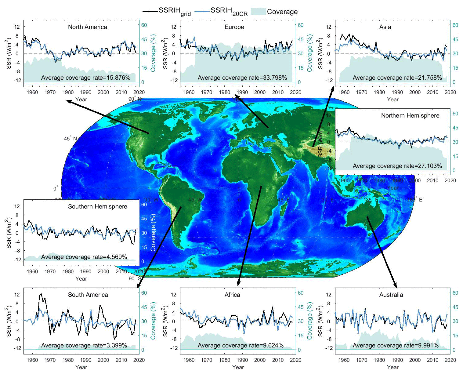
Figure 9Same as Fig. 8 but for regional annual anomaly variations.
Figure 9 demonstrates the long-term annual anomaly variations of the SSRIH20CR in different regions and its results compared to the SSRIHgrid. Table S4 in the Supplement shows the evaluation in continental and hemispheric SSRIH20CR change trends on different scales. The SSRIH20CR shows a similar annual anomaly variation to the global land (except for Antarctica) average trend in North America and Asia, reaches a minimum in the late 1970s or early 1990s, and follows a moderate reversal. In Europe, the SSRIH20CR shows a decrease (−2.180 ± 1.866 W m−2 per decade) between 1963 and 1978 before turning to brightening (1.081 ± 0.312 W m−2 per decade). In South America and Australia (Southern Hemisphere), the SSRIH20CR shows no significant variation. In Africa, the SSRIH20CR has a dimming trend (−1.506 ± 0.496 W m2 per decade) from the 1950s to the 1990s, after which it remains levelled off (0.340 ± 0.998 W m−2 per decade). The SSRIH20CR shows a decreasing trend (−1.457 ± 0.246 W m−2 per decade) until the 1990s in the Northern Hemisphere and a brightening (0.887 ± 0.415 W m−2 per decade) afterwards. The annual average anomaly variations in regions and globally show that Asia, Africa, Europe and North America are the four contributors to the global dimming, while Europe and North America are two major contributors to the brightening. This is in general agreement with the results obtained by previous machine learning (Yuan et al., 2021). In addition, the discrepancy between the SSRIH20CR and SSRIHgrid is more significant in low-coverage areas (right) than in high-coverage regions (left). It is particularly pronounced before 1980 and in South America. This suggests that the limited surface observations are not representative of the continental variation in SSR.
The sources of error in the observational dataset can be divided into three types. (1) Station errors are the uncertainties of individual station anomalies, including measurement errors (which are not the focus of the considerations in this paper) and errors due to homogenization. The errors due to homogenization adjustment are always approximately normally distributed (Jones et al., 2008; see their Fig. 5 and Fig. S9 in the Supplement) and therefore have limited impacts on the global average SSR change (Fig. S5a, b). (2) Sampling errors are the uncertainties in a grid box mean caused by estimating the mean from a small number of point values (Jones et al., 1997). (3) Bias error generally refers to systematic errors such as urbanization, which has not been discussed here. However, even the sum of the above errors is much smaller than the errors due to limited data coverage (Li et al., 2010; see their Fig. 5). So, the focus of this study is to eliminate this kind of error through the CNN reconstruction.
Both the SSRIHgrid (the homogenized monthly gridded SSR data over 1923–2020) and the SSRIH20CR (the monthly 20CR-AI model reconstructed SSR data for 1955–2018) are currently publicly available on the figshare website at https://doi.org/10.6084/m9.figshare.21625079.v1 (Jiao and Li, 2023). These datasets are also available at http://www.gwpu.net (last access: May 2023) for free.
In this study, we integrate global station observations based on the raw observational SSRs from GEBA and WRDC, combined with existing homogenized SSR datasets from other scholars. Also, we homogenize the globally distributed station data using the RHtestV4 software package. An improved CNN deep-learning algorithm is subsequently used to reconstruct the SSR anomalies. Thus, a reconstructed SSR anomaly dataset, SSRIH20CR, is obtained based on training sets (20CRv3) for the years 1955–2018, with a resolution of 5∘ × 2.5∘. The main results are as follows.
-
The first integrated and homogenized global SSR monthly dataset is developed, which contains 944 stations in total and covers the longest periods (from the 1920s to recent years). A 5∘ × 5∘ grid box version of the monthly SSR anomaly dataset is derived.
-
This paper develops 5∘ × 2.5∘ full-coverage monthly land (except for Antarctica) SSR anomaly reconstructed datasets based on the above observations, using 20CRv3 to train the AI model. Comparative validations and evaluations show that the SSRIH20CR provides a reliable benchmark for global SSR variations.
-
On average, the global annual SSR variations based on the SSRIHgrid are not significantly different, except that the increasing (brightening) trend after 1991 is a little smaller for the latter. The short-term brightening SSR in Europe from the 1970s to the 1980s disappears at the regional scale. At the same time, the brightening SSR after the 1990s in Asia slowed or was delayed.
The supplement related to this article is available online at: https://doi.org/10.5194/essd-15-4519-2023-supplement.
BJ: software, data curation, writing – original draft preparation, visualization, investigation. YS: software, data curation. QL: methodology, supervision, conceptualization, validation, writing – review and editing. VM: provision of the homogenized Italian dataset, writing – review and editing. MW: writing – review and editing.
At least one of the (co-)authors is a member of the editorial board of Earth System Science Data. The peer-review process was guided by an independent editor, and the authors also have no other competing interests to declare.
Publisher's note: Copernicus Publications remains neutral with regard to jurisdictional claims in published maps and institutional affiliations.
This research has been supported by the Natural Science Foundation of China (grant no. 41975105) and the National Key R&D Program of China (grant nos. 2018YFC1507705 and 2017YFC1502301). The Global Energy Balance Archive (GEBA) is co-funded by the Federal Office of Meteorology and Climatology (MeteoSwiss) within the framework of GCOS Switzerland. Global dimming and brightening research at ETH Zurich is supported by the Swiss National Science Foundation (grant no. 200020 188601). Veronica Manara was supported by the Ministero dell'Università e della Ricerca of Italy (grant FSE – REACT EU, DM 10/08/2021 n. 1062).
This study is supported by the Natural Science Foundation of China (grant no. 41975105) and the National Key R&D Program of China (grant nos. 2018YFC1507705 and 2017YFC1502301). The Global Energy Balance Archive (GEBA) is co-funded by the Federal Office of Meteorology and Climatology (MeteoSwiss) within the framework of GCOS Switzerland. Global dimming and brightening research at ETH Zurich is supported by the Swiss National Science Foundation (grant no. 200020 188601). Veronica Manara was supported by the Ministero dell'Università e della Ricerca of Italy (grant FSE – REACT EU, DM 10/08/2021 n. 1062).
This paper was edited by Jing Wei and reviewed by two anonymous referees.
Aguiar, L. M., Pereira, B., David, M., Díaz, F., and Lauret, P.: Use of satellite data to improve solar radiation forecasting with Bayesian Artificial Neural Networks, Sol. Energy, 122, 1309–1324, https://doi.org/10.1016/j.solener.2015.10.041, 2015.
Alexandersson, H.: A homogeneity test applied to precipitation data, J. Climatol., 6, 661–675, https://doi.org/10.1002/joc.3370060607, 1986.
Bookstein, F. L.: Principal warps: Thin-plate splines and the decomposition of deformations, IEEE T. Pattern Anal., 11, 567–585, https://doi.org/10.1109/34.24792, 1989.
Brohan, P., Kennedy, J. J., Harris, I., Tett, S. F. B., and Jones, P. D.: Uncertainty estimates in regional and global observed temperature changes: A new data set from 1850, J. Geophys. Res.-Atmos., 111, D12106m https://doi.org/10.1029/2005JD006548, 2006.
Collins, F. C.: A comparison of spatial interpolation techniques in temperature estimation, The 3rd International Conference/Workshop on Integrating GIS and Environmental Modeling, Santa Barbara, Santa Fe, NM; Santa Barbara, CA, 21–26 January 1996.
Craddock, J. M.: Methods of comparing annual rainfall records for climatic purposes, Weather, 34, 332–346, https://doi.org/10.1002/j.1477-8696.1979.tb03465.x, 1979.
Driemel, A., Augustine, J., Behrens, K., Colle, S., Cox, C., Cuevas-Agulló, E., Denn, F. M., Duprat, T., Fukuda, M., Grobe, H., Haeffelin, M., Hodges, G., Hyett, N., Ijima, O., Kallis, A., Knap, W., Kustov, V., Long, C. N., Longenecker, D., Lupi, A., Maturilli, M., Mimouni, M., Ntsangwane, L., Ogihara, H., Olano, X., Olefs, M., Omori, M., Passamani, L., Pereira, E. B., Schmithüsen, H., Schumacher, S., Sieger, R., Tamlyn, J., Vogt, R., Vuilleumier, L., Xia, X., Ohmura, A., and König-Langlo, G.: Baseline Surface Radiation Network (BSRN): structure and data description (1992–2017), Earth Syst. Sci. Data, 10, 1491–1501, https://doi.org/10.5194/essd-10-1491-2018, 2018.
Erxleben, J., Elder, K., and Davis, R.: Comparison of spatial interpolation methods for estimating snow distribution in the Colorado Rocky Mountains, Hydrol. Process., 16, 3627–3649, https://doi.org/10.1002/hyp.1239, 2002.
Evan, A. T., Heidinger, A. K., and Vimont, D. J.: Arguments against a physical long-term trend in global ISCCP cloud amounts, Geophys. Res. Lett., 34, L04701m https://doi.org/10.1029/2006gl028083, 2007.
Eyring, V., Bony, S., Meehl, G. A., Senior, C. A., Stevens, B., Stouffer, R. J., and Taylor, K. E.: Overview of the Coupled Model Intercomparison Project Phase 6 (CMIP6) experimental design and organization, Geosci. Model Dev., 9, 1937–1958, https://doi.org/10.5194/gmd-9-1937-2016, 2016.
Feng, F. and Wang, K.: Merging high-resolution satellite surface radiation data with meteorological sunshine duration observations over China from 1983 to 2017, Remote Sens., 13, 602, https://doi.org/10.3390/rs13040602, 2021.
Fisher, N. I., Lewis, T., and Embleton, B. J.: Statistical analysis of spherical data, Cambridge University Press, https://doi.org/10.1017/CBO9780511623059, 1993.
Fukami, K., Fukagata, K., and Taira, K.: Machine-learning-based spatio-temporal super resolution reconstruction of turbulent flows, J. Fluid Mech., 909, A9-1–A9-14, https://doi.org/10.1017/jfm.2020.948, 2021.
Gates, W. L., Boyle, J. S., Covey, C., Dease, C. G., Doutriaux, C. M., Drach, R. S., Fiorino, M., Gleckler, P. J., Hnilo, J. J., Marlais, S. M., Phillips, T. J., Potter, G. L., Santer, B. D., Sperber, K. R., Taylor, K. E., and Williams, D. N.: An Overview of the Results of the Atmospheric Model Intercomparison Project (AMIP I), B. Am. Meteorol. Soc., 80, 29–55, https://doi.org/10.1175/1520-0477(1999)080<0029:Aootro>2.0.Co;2, 1999.
Gulev, S. K., Thorne, P. W., J. Ahn, F. J. D., Domingues, C. M., Gerland, S., Gong, D., Kaufman, D. S., Nnamchi, H. C., Quaas, J., Rivera, J. A., Sathyendranath, S., Smith, S. L., Trewin, B., von Shuckmann, K., and Vose, R. S.: Changing State of the Climate System. In Climate Change 2021: The Physical Science Basis. Contribution of Working Group I to the Sixth Assessment Report of the Intergovernmental Panel on Climate Change, edited by: Masson-Delmotte, V., Zhai, P., Pirani, A., Connors, S. L., Péan, C., Berger, S., Caud, N., Chen, Y., Goldfarb, L., Gomis, M. I., Huang, M., Leitzell, K., Lonnoy, E., Matthews, J. B. R., Maycock, T. K., Waterfield, T., Yelekçi, O., Yu, R., and Zhou, B., Cambridge University Press, 287–422, https://doi.org/10.1017/9781009157896.004, 2021.
He, J., Hong, L., Shao, C., and Tang, W.: Global evaluation of simulated surface shortwave radiation in CMIP6 models, Atmos. Res., 292, 106896, https://doi.org/10.1016/j.atmosres.2023.106896, 2023.
He, Y., Wang, K., and Feng, F.: Improvement of ERA5 over ERA-Interim in simulating surface incident solar radiation throughout China, J. Climate, 34, 3853–3867, 2021.
Hersbach, H., Bell, B., Berrisford, P., Hirahara, S., Horányi, A., Muñoz-Sabater, J., Nicolas, J., Peubey, C., Radu, R., Schepers, D., Simmons, A., Soci, C., Abdalla, S., Abellan, X., Balsamo, G., Bechtold, P., Biavati, G., Bidlot, J. R., Bonavita, M., Chiara, G. D., Dahlgren, P., Dee, D., Diamantakis, M., Dragani, R., Flemming, J., Forbes, R. G., Fuentes, M., Geer, A. J., Haimberger, L., Healy, S. B., Hogan, R. J., Holm, E. V., Janisková, M., Keeley, S. P. E., Laloyaux, P., Lopez, P., Lupu, C., Radnoti, G., de Rosnay, P., Rozum, I., Vamborg, F., Villaume, S., and Thepaut, J.-N.: The ERA5 global reanalysis, Q. J. Roy. Meteor. Soc., 146, 1999–2049, https://doi.org/10.1002/qj.3803, 2020.
Hoskins, B. J. and Valdes, P. J.: On the existence of storm-tracks, J. Atmos. Sci., 47, 1854–1864, https://doi.org/10.1175/1520-0469(1990)047<1854:OTEOST>2.0.CO;2, 1990.
Huang, B., Yin, X., Menne, M. J., Vose, R., and Zhang, H.-M.: Improvements to the Land Surface Air Temperature Reconstruction in NOAAGlobalTemp: An Artificial Neural Network Approach, Artificial Intelligence for the Earth Systems, 1 1–35, https://doi.org/10.1175/AIES-D-22-0032.1, 2022.
Huang, J., Rikus, L. J., Qin, Y., and Katzfey, J.: Assessing model performance of daily solar irradiance forecasts over Australia, Sol. Energy, 176, 615–626, https://doi.org/10.1016/j.solener.2018.10.080, 2018.
Jiao, B. and Li, Q.: Global Integrated and Homogenized Solar surface Radiation Datasets, figshare [data set], https://doi.org/10.6084/m9.figshare.21625079.v1, 2023.
Jiao, B., Li, Q., Sun, W., and Martin, W.: Uncertainties in the global and continental surface solar radiation variations: inter-comparison of in-situ observations, reanalyses, and model simulations, Clim. Dynam., 59, 2499–2516, https://doi.org/10.1007/s00382-022-06222-3, 2022.
Jones, P., Osborn, T., Briffa, K., Folland, C., Horton, E., Alexander, L., Parker, D., and Rayner, N.: Adjusting for sampling density in grid box land and ocean surface temperature time series, J. Geophys. Res.-Atmos., 106, 3371–3380, https://doi.org/10.1029/2000JD900564, 2001.
Jones, P. D., Osborn, T. J., and Briffa, K. R.: Estimating Sampling Errors in Large-Scale Temperature Averages, J. Climate, 10, 2548–2568, 1997.
Jones, P. D., Lister, D. H., and Li, Q.: Urbanization effects in large-scale temperature records, with an emphasis on China, J. Geophys. Res., 113, D16122, https://doi.org/10.1029/2008jd009916, 2008.
Ju, X., Tu, Q., and Li, Q.: Homogeneity test and reduction of monthly total solar radiation over China, J. Nanjing Inst. Meteorol., 29, 336–341, 2006.
Kadow, C., Hall, D. M., and Ulbrich, U.: Artificial intelligence reconstructs missing climate information, Nat. Geosci., 13, 408–413, https://doi.org/10.1038/s41561-020-0582-5, 2020.
Kambezidis, H. D., Kaskaoutis, D. G., Kharol, S. K., Moorthy, K. K., Satheesh, S. K., Kalapureddy, M. C. R., Badarinath, K. V. S., Sharma, A. R., and Wild, M.: Multi-decadal variation of the net downward shortwave radiation over south Asia: The solar dimming effect, Atmos. Environ., 50, 360–372, 2012.
Krige, D. G.: A statistical approach to some basic mine valuation problems on the Witwatersrand, J. S. Afr. I. Min. Metall., 52, 119–139, https://doi.org/10.10520/AJA0038223X_4792, 1951.
Leirvik, T. and Yuan, M.: A machine learning technique for spatial interpolation of solar radiation observations, Earth Space Sci., 8, e2020EA001527, https://doi.org/10.1029/2020EA001527, 2021.
Li, Q., Dong, W., Li, W., Gao, X., Jones, P., Kennedy, J., and Parker, D.: Assessment of the uncertainties in temperature change in China during the last century, Chinese Sci. Bull., 55, 1974–1982, 10.1007/s11434-010-3209-1, 2010.
Li, Q., Sun, W., Yun, X., Huang, B., Dong, W., Wang, X. L., Zhai, P., and Jones, P.: An updated evaluation of the global mean land surface air temperature and surface temperature trends based on CLSAT and CMST, Clim. Dynam., 56, 635–650, https://doi.org/10.1007/s00382-020-05502-0, 2021.
Liang, H., Jiang, B., Liang, S., Peng, J., Li, S., Han, J., Yin, X., Cheng, J., Jia, K., and Liu, Q.: A global long-term ocean surface daily/0.05∘ net radiation product from 1983–2020, Sci. Data, 9, 1–17, https://doi.org/10.1038/s41597-022-01419-x, 2022.
Ma, Q., Wang, K., He, Y., Su, L., Wu, Q., Liu, H., and Zhang, Y.: Homogenized century-long surface incident solar radiation over Japan, Earth Syst. Sci. Data, 14, 463–477, https://doi.org/10.5194/essd-14-463-2022, 2022.
Manara, V., Brunetti, M., Celozzi, A., Maugeri, M., Sanchez-Lorenzo, A., and Wild, M.: Detection of dimming/brightening in Italy from homogenized all-sky and clear-sky surface solar radiation records and underlying causes (1959–2013), Atmos. Chem. Phys., 16, 11145–11161, https://doi.org/10.5194/acp-16-11145-2016, 2016.
Manara, V., Brunetti, M., Maugeri, M., Sanchez-Lorenzo, A., and Wild, M.: Homogenization of a surface solar radiation dataset over Italy, AIP Conference Proceedings, 1810, 090004, https://doi.org/10.1063/1.4975544, 2017.
Manara, V., Bassi, M., Brunetti, M., Cagnazzi, B., and Maugeri, M.: 1990–2016 surface solar radiation variability and trend over the Piedmont region (northwest Italy), Theor. Appl. Climatol., 136, 849–862, https://doi.org/10.1007/s00704-018-2521-6, 2019.
Manara, V., Stocco, E., Brunetti, M., Diolaiuti, G. A., Fugazza, D., Pfeifroth, U., Senese, A., Trentmann, J., and Maugeri, M.: Comparison of Surface Solar Irradiance from Ground Observations and Satellite Data (1990–2016) over a Complex Orography Region (Piedmont—Northwest Italy), Remote Sens, 12, 3882, https://doi.org/10.3390/rs12233882, 2020.
Mlawer, E. J., Taubman, S. J., Brown, P. D., Iacono, M. J., and Clough, S. A.: Radiative transfer for inhomogeneous atmospheres: RRTM, a validated correlated-k model for the longwave, J. Geophys. Res.-Atmos., 102, 16663–16682, https://doi.org/10.1029/97JD00237, 1997.
Olanow, C. W. and Koller, W. C.: An algorithm (decision tree) for the management of Parkinson's disease: Treatment guidelines, Neurology, 50, S1–S88, 1998.
Padma Kumari, B., Londhe, A. L., Daniel, S., and Jadhav, D. B.: Observational evidence of solar dimming: Offsetting surface warming over India, Geophys. Res. Lett., 34, L21810, https://doi.org/10.1029/2007GL031133, 2007.
Peixoto, J. P., Oort, A. H., and Lorenz, E. N.: Physics of climate, Springer, ISBN 978-0-88318-712-8, 1992.
Peterson, T. C., Karl, T. R., Jamason, P. F., Knight, R., and Easterling, D. R.: First difference method: Maximizing station density for the calculation of long-term global temperature change, J. Geophys. Res.-Atmos., 103, 25967–25974, https://doi.org/10.1029/98JD01168, 1998.
Pfeifroth, U., Sanchez-Lorenzo, A., Manara, V., Trentmann, J., and Hollmann, R.: Trends and Variability of Surface Solar Radiation in Europe Based On Surface- and Satellite-Based Data Records, J. Geophys. Res.-Atmos., 123, 1735–1754, https://doi.org/10.1002/2017JD027418, 2018.
Ronneberger, O., Fischer, P., and Brox, T.: U-net: Convolutional networks for biomedical image segmentation, International Conference on Medical image computing and computer-assisted intervention, arXiv [preprint], 234–241, https://doi.org/10.48550/arXiv.1505.04597, 2015.
Sanchez-Lorenzo, A., Calbó, J., and Wild, M.: Global and diffuse solar radiation in Spain: Building a homogeneous dataset and assessing their trends, Global Planet. Change, 100, 343–352, https://doi.org/10.1016/j.gloplacha.2012.11.010, 2013a.
Sanchez-Lorenzo, A., Wild, M., and Trentmann, J.: Validation and stability assessment of the monthly mean CM SAF surface solar radiation dataset over Europe against a homogenized surface dataset (1983–2005), Remote Sens. Environ., 134, 355–366, https://doi.org/10.1016/j.rse.2013.03.012, 2013b.
Sanchez-Lorenzo, A., Wild, M., Brunetti, M., Guijarro, J. A., Hakuba, M. Z., Calbó, J., Mystakidis, S., and Bartok, B.: Reassessment and update of long-term trends in downward surface shortwave radiation over Europe (1939–2012), J. Geophys. Res.-Atmos., 120, 9555–9569, https://doi.org/10.1002/2015JD023321, 2015.
Scudiero, E., Corwin, D. L., Morari, F., Anderson, R. G., and Skaggs, T. H.: Spatial interpolation quality assessment for soil sensor transect datasets, Comput. Electron. Agr., 123, 74–79, https://doi.org/10.1016/j.compag.2016.02.016, 2016.
Shao, C., Yang, K., Tang, W., He, Y., Jiang, Y., Lu, H., Fu, H., and Zheng, J.: Convolutional neural network-based homogenization for constructing a long-term global surface solar radiation dataset, Renew. Sust. Energ. Rev., 169, 112952, https://doi.org/10.1016/j.rser.2022.112952, 2022.
Shepard, D.: A two-dimensional interpolation function for irregularly-spaced data, Proceedings of the 1968 23rd ACM national conference, 517–524, https://doi.org/10.1145/800186.810616, 1068.
Slivinski, L. C., Compo, G. P., Whitaker, J. S., Sardeshmukh, P. D., Giese, B. S., McColl, C., Allan, R., Yin, X., Vose, R., and Titchner, H.: Towards a more reliable historical reanalysis: Improvements for version 3 of the Twentieth Century Reanalysis system, Q. J. Roy. Meteor. Soc., 145, 2876–2908, https://doi.org/10.1002/qj.3598, 2019.
Soni, V. K., Pandithurai, G., and Pai, D. S.: Evaluation of long-term changes of solar radiation in India, Int. J. Climatol., 32, 540–551, https://doi.org/10.1002/joc.2294, 2012.
Soni, V. K., Pandithurai, G., and Pai, D. S.: Is there a transition of solar radiation from dimming to brightening over India, Atmos. Res., 169, 209-224, 2016.
Tang, W., Qin, J., Yang, K., Liu, S., Lu, N., and Niu, X.: Retrieving high-resolution surface solar radiation with cloud parameters derived by combining MODIS and MTSAT data, Atmos. Chem. Phys., 16, 2543–2557, https://doi.org/10.5194/acp-16-2543-2016, 2016.
Tang, W., Yang, K., Qin, J., Li, X., and Niu, X.: A 16-year dataset (2000–2015) of high-resolution (3 h, 10 km) global surface solar radiation, Earth Syst. Sci. Data, 11, 1905–1915, https://doi.org/10.5194/essd-11-1905-2019, 2019.
Trenberth, K. E. and Fasullo, J. T.: Regional energy and water cycles: Transports from ocean to land, J. Climate, 26, 7837–7851, https://doi.org/10.1175/JCLI-D-13-00008.1, 2013.
Tsvetkov, A., Wilcox, S., Renne, D., and Pulscak, M.: International solar resource data at the World Radiation Data Center, American Solar Energy Society, Boulder, CO (United States), ISBN 0-89553-167-4, 1995.
Urraca, R., Huld, T., Martinez-de-Pison, F. J., and Sanz-Garcia, A.: Sources of uncertainty in annual global horizontal irradiance data, Sol. Energy, 170, 873–884, https://doi.org/10.1016/j.solener.2018.06.005, 2018.
Vincent, L. A., Wang, X. L., Milewska, E. J., Wan, H., Yang, F., and Swail, V.: A second generation of homogenized Canadian monthly surface air temperature for climate trend analysis, J. Geophys. Res.-Atmos., 117, D18110, https://doi.org/10.1029/2012JD017859, 2012.
Wang, K.: Measurement biases explain discrepancies between the observed and simulated decadal variability of surface incident solar radiation, Sci. Rep., 4, 1–7, https://doi.org/10.1038/srep06144, 2014.
Wang, K., Ma, Q., Li, Z., and Wang, J.: Decadal variability of surface incident solar radiation over China: Observations, satellite retrievals, and reanalyses, J. Geophys. Res.-Atmos., 120, 6500–6514, https://doi.org/10.1002/2015JD023420, 2015.
Wang, X. L.: Accounting for autocorrelation in detecting mean shifts in climate data series using the penalized maximal t or F test, J. Appl. Meteorol. Clim., 47, 2423–2444, https://doi.org/10.1175/2008JAMC1741.1, 2008a.
Wang, X. L.: Penalized maximal F test for detecting undocumented mean shift without trend change, J. Atmos. Ocean. Tech., 25, 368–384, https://doi.org/10.1175/2007JTECHA982.1, 2008b.
Wang, X. L. and Feng, Y.: RHtestsV4 user manual, Climate Research Division, Atmospheric Science and Technology Directorate, Science and Technology Branch, Environment Canada, 28, 2013.
Wang, X. L., Wen, Q. H., and Wu, Y.: Penalized maximal t test for detecting undocumented mean change in climate data series, J. Appl. Meteorol. Clim., 46, 916–931, https://doi.org/10.1175/JAM2504.1, 2007.
Wang, X. L., Chen, H., Wu, Y., Feng, Y., and Pu, Q.: New techniques for the detection and adjustment of shifts in daily precipitation data series, J. Appl. Meteorol. Clim., 49, 2416–2436, https://doi.org/10.1175/2010JAMC2376.1, 2010.
Wang, Y. and Wild, M.: A new look at solar dimming and brightening in China, Geophys. Res. Lett., 43, 11777–711785, https://doi.org/10.1002/2016GL071009, 2016.
Wild, M.: Enlightening global dimming and brightening, B. Am. Meteorol. Soc., 93, 27–37, https://doi.org/10.1175/BAMS-D-11-00074.1, 2012.
Wild, M.: The global energy balance as represented in CMIP6 climate models, Clim. Dynam., 55, 553–577, https://doi.org/10.1007/s00382-020-05282-7, 2020.
Wild, M., Gilgen, H., Roesch, A., Ohmura, A., Long, C. N., Dutton, E. G., Forgan, B., Kallis, A., Russak, V., and Tsvetkov, A.: From dimming to brightening: Decadal changes in solar radiation at Earth's surface, Science, 308, 847–850, https://doi.org/10.1126/science.1103215, 2005.
Wild, M., Trüssel, B., Ohmura, A., Long, C. N., König-Langlo, G., Dutton, E. G., and Tsvetkov, A.: Global dimming and brightening: An update beyond 2000, J. Geophys. Res.-Atmos., 114, D011382, https://doi.org/10.1029/2008JD011382, 2009.
Wild, M., Ohmura, A., Schär, C., Müller, G., Folini, D., Schwarz, M., Hakuba, M. Z., and Sanchez-Lorenzo, A.: The Global Energy Balance Archive (GEBA) version 2017: a database for worldwide measured surface energy fluxes, Earth Syst. Sci. Data, 9, 601–613, https://doi.org/10.5194/essd-9-601-2017, 2017.
Xu, W., Li, Q., Wang, X. L., Yang, S., Cao, L., and Feng, Y.: Homogenization of Chinese daily surface air temperatures and analysis of trends in the extreme temperature indices, J. Geophys. Res.-Atmos., 118, 9708–9720, https://doi.org/10.1002/jgrd.50791, 2013.
Xu, W., Li, Q., Jones, P., Wang, X. L., Trewin, B., Yang, S., Zhu, C., Zhai, P., Wang, J., and Vincent, L.: A new integrated and homogenized global monthly land surface air temperature dataset for the period since 1900, Clim. Dynam., 50, 2513–2536, https://doi.org/10.1007/s00382-017-3755-1, 2018.
Yang, L., Zhang, X., Liang, S., Yao, Y., Jia, K., and Jia, A.: Estimating surface downward shortwave radiation over China based on the gradient boosting decision tree method, Remote Sens., 10, 185, https://doi.org/10.3390/rs10020185, 2018.
Yang, S., Wang, X. L., and Wild, M.: Homogenization and trend analysis of the 1958–2016 in situ surface solar radiation records in China, J. Climate, 31, 4529–4541, https://doi.org/10.1175/JCLI-D-17-0891.1, 2018.
You, Q., Sanchez-Lorenzo, A., Wild, M., Folini, D., Fraedrich, K., Ren, G., and Kang, S.: Decadal variation of surface solar radiation in the Tibetan Plateau from observations, reanalysis and model simulations, Clim. Dynam., 40, 2073–2086, https://doi.org/10.1007/s00382-012-1383-3, 2013.
Yuan, M., Leirvik, T., and Wild, M.: Global trends in downward surface solar radiation from spatial interpolated ground observations during 1961–2019, J. Climate, 34, 9501–9521, https://doi.org/10.1175/JCLI-D-21-0165.1, 2021.
Zhou, C., Wang, K., and Ma, Q.: Evaluation of Eight Current Reanalyses in Simulating Land Surface Temperature from 1979 to 2003 in China, J. Climate, 30, 7379–7398, https://doi.org/10.1175/JCLI-D-16-0903.1, 2017.
Zhou, C., He, Y., and Wang, K.: On the suitability of current atmospheric reanalyses for regional warming studies over China, Atmos. Chem. Phys., 18, 8113–8136, https://doi.org/10.5194/acp-18-8113-2018, 2018.
Zhou, W., Gong, L., Wu, Q., Xing, C., Wei, B., Chen, T., Zhou, Y., Yin, S., Jiang, B., Xie, H., Zhou, L., and Zheng, S.: Correction to: PHF8 upregulation contributes to autophagic degradation of E-cadherin, epithelial-mesenchymal transition and metastasis in hepatocellular carcinoma, J. Exp. Clin. Canc. Res., 37, 445, https://doi.org/10.1186/s13046-018-0944-7, 2018.
Zhou, W., Gong, L., Wu, Q., Xing, C., Wei, B., Chen, T., Zhou, Y., Yin, S., Jiang, B., Xie, H., Zhou, L., and Zheng, S.: Correction to: PHF8 upregulation contributes to autophagic degradation of E-cadherin, epithelial-mesenchymal transition and metastasis in hepatocellular carcinoma, J. Exp. Clin. Canc. Res., 38, 445, https://doi.org/10.1186/s13046-019-1452-0, 2019.