Hydro-PE: gridded datasets of historical and future Penman–Monteith potential evaporation for the United Kingdom

We present two new potential evaporation datasets for the United Kingdom: a historical dataset, Hydro-PE HadUK-Grid, which is derived from the HadUK-Grid gridded observed meteorology (1969–2021), and a future dataset, Hydro-PE UKCP18 RCM, which is derived from UKCP18 regional climate projections (1980–2080). Both datasets are suitable for hydrological modelling and provide Penman–Monteith potential evapotranspiration parameterised for short grass, with and without a correction for interception on days with rainfall. The potential evapotranspiration calculations have been formulated to closely follow the methodology of the existing Meteorological Office Rainfall and Evaporation Calculation System (MORECS) potential evapotranspiration, which has historically been widely used by hydrological modellers in the United Kingdom. The two datasets have been created using the same methodology to allow seamless modelling from past to future. Hydro-PE HadUK-Grid shows good agreement with MORECS in much of the United Kingdom, although Hydro-PE HadUK-Grid is higher in the mountainous regions of Scotland and Wales. This is due to differences in the underlying meteorology, in particular the wind speed, which are themselves due to the different spatial scales of the data. Hydro-PE HadUK-Grid can be downloaded from https://doi.org/10.5285/9275ab7e-6e93-42bc-8e72-59c98d409deb (Brown et al., 2022) and Hydro-PE UKCP18 RCM can be downloaded from https://doi.org/10.5285/eb5d9dc4-13bb-44c7-9bf8-c5980fcf52a4 (Robinson et al., 2021).

1 Introduction

Evaporation is an important part of the hydrological cycle. Globally it is estimated that around 60 % of the precipitation that falls on the land is returned to the atmosphere by evaporation from the land (Abbott et al., 2019). However, evaporation is difficult to observe, particularly over large areas, so estimates of potential evaporation (PE) can instead be derived from observed meteorology. PE is an estimate of the evaporative demand of the atmosphere, given an assumed land cover, and is a measure of how much evaporation would occur under specific meteorological conditions given an unlimited water supply in the soil. In hydrological and crop modelling the actual evaporation (AE) from the land is calculated using PE as an estimate of the unlimited evaporation flux, scaled by a function of the soil wetness (Federer et al., 1996). Therefore PE is an essential driving input for hydrological models, and accurate estimation of PE is essential for model performance, particularly in regions where rainfall is not limiting (Kay et al., 2013).

Evaporation from the land can include evaporation from the water contained in the soil, through either transpiration (evaporation through plant stomata) or evaporation from the soil surface directly and through evaporation from open water surfaces (either from permanent water bodies such as lakes or from transient water on the surface of vegetation or ponding). In this paper we refer to the potential evaporation from the soil as potential evapotranspiration (PET), which may include both transpiration and evaporation from the bare soil. We refer to PE products that also include evaporation from water intercepted by the vegetation canopy as potential evapotranspiration with interception (PETI). We use PE as a catch-all term for both of these. The units of PE can be given as a mass flux (kg m⁻² d⁻¹) or the equivalent depth of water (mm d⁻¹, assuming a water density of 1000 kg m⁻³). These are numerically equivalent. In this paper, we use millimetres per day.

There are a variety of formulations of PE that rely on various combinations of meteorological inputs. The most parsimonious use just one (e.g. Thornthwaite, 1948; Oudin et al., 2005) or two (e.g. Blaney and Criddle, 1950; Priestley and Taylor, 1972) meteorological variables but rely on empirical factors which are calibrated to historical or present-day climates. Different formulations of PE can show different trends under a changing climate, adding to the uncertainty of climate change impacts on hydrology (Lemaitre-Basset et al., 2022). The more complex Penman–Monteith formulation (Monteith, 1965), while requiring a larger number of observed inputs, is derived from fundamental physics and so is able to represent temporal changes in drivers. Additionally, PE is influenced by physical and physiological properties of the land surface, e.g. leaf area, plant height, albedo or emissivity. These properties are implicitly part of the empirical parameterisation of the simpler models of PE but can be explicitly included in the calculation of Penman–Monteith PE. Since both the meteorology and the properties of the land surface can be expected to change in the future, Penman–Monteith is most suitable as an input for hydrological modelling in a changing climate (Lemaitre-Basset et al., 2022).

Under climate change, the warming of the atmosphere is expected to intensify the hydrological cycle, with a warmer atmosphere able to hold more water, leading to increased evaporation and precipitation (Trenberth, 1999). Alongside this, the rise in atmospheric CO₂ concentrations is expected to lead to stomatal closure in plants, which would lead to increased water use efficiency and decreased transpiration per unit leaf area (Cao et al., 2010). However, it may also lead to increased plant growth, which would mean more transpiring leaf surface per unit area of ground (Alo and Wang, 2008). These are several possibly compensating effects that can all be captured by the Penman–Monteith equation (Donohue et al., 2010).

The estimation of PE is highly dependent on land use, so any PE must be quoted for a specific parameterisation of the land cover and vegetation. To standardise this, the concept of a “reference crop” was introduced, usually short grass as recommended by the United Nations Food and Agricultural Organisation (FAO) (Pereira et al., 1999). Although some PE products are provided for different land covers, for many products, a short-grass parameterisation is assumed.

In the temperate maritime climate of the United Kingdom (UK), land evaporation is estimated to be around 40 % of land precipitation, based on observed river flow (Hannaford, 2015) and modelled runoff and evaporation (Blyth et al., 2019). It can be as high as 60 % in the water-limited regions of England and as low as 30 % in the cooler, wetter regions of Scotland and Wales (Blyth et al., 2019). Widely used PE datasets for hydrological modelling in the UK include MORECS PE, a 40 km gridded product for various land covers (Hough et al., 1997); MOSES, a 5 km gridded product calculated by the MOSES land surface model (Cox et al., 1998; Smith et al., 2006); and CHESS-PE, a 1 km gridded product for time-invariant short grass (Robinson et al., 2017) that has been aggregated to the catchment scale as a component of the CAMELS-GB dataset (Coxon et al., 2020b, a). The FAO reference evapotranspiration method provides a formulation for calculating PE using local observed data, including a variety of adaptations to accommodate differing levels of data availability (Allen et al., 1998). MORECS PE calculated for short grass is the most widely used in hydrological modelling in the UK and so is considered a reference dataset throughout this paper. A comparison of PE products can be seen in Table 1.

(Hough and Jones, 1997)(Robinson et al., 2017)(Smith et al., 2006)(Allen et al., 1998)

Table 1 Existing Penman–Monteith PE datasets and methods available in the UK.

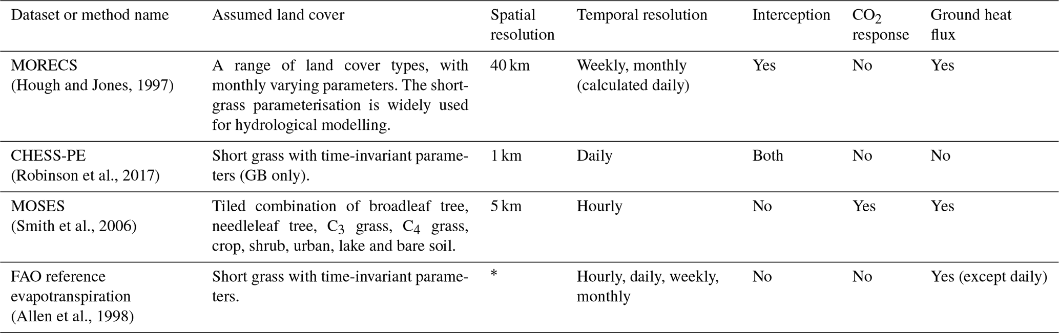
^* FAO is a method rather than a specific dataset. It can be applied to site or spatial data.

The MORECS PE dataset is provided by the UK Met Office for near-real-time and historical hydrological and crop modelling in the UK (Hough et al., 1997; Hough and Jones, 1997). It is a gridded estimate of weekly and monthly mean PE at 40 km resolution derived from the MORECS 40 km gridded meteorological dataset. The gridded meteorology is interpolated from a network of meteorological observation stations before being used to calculate PE. It has been widely used as an input for hydrological models, both for research and operationally (Kay et al., 2013). MORECS PE is calculated for a reference short grass and several other land covers. Some hydrological models use the short-grass MORECS PE and apply an adjustment for known land cover (e.g. CLASSIC, Crooks and Naden, 2007). MORECS is purely observation-based and has no corollary for studies of hydrology under future climate. It is also only available at a much lower resolution (40 km) than the typical resolution (1 km) of hydrological models (Bell et al., 2009; Crooks and Naden, 2007) and available rainfall datasets (Met Office et al., 2021; Tanguy et al., 2021; Lewis et al., 2022) in the UK. Since potential evapotranspiration is a non-linear function of the meteorology, using a lower-resolution PE potentially misses important effects of local topography.

MORECS PE uses the Penman–Monteith formulation (Hough et al., 1997) but with some modifications. It includes a correction for the assumption that the surface temperature is equal to the air temperature, uses monthly varying physiological parameters (leaf area index and stomatal resistance), and implements a correction on rain days to account for interception. This latter interception correction is important for driving models which do not explicitly calculate interception. Since interception is more efficient than transpiration, this combined PETI is higher than PET alone. The difference can be of the order of 10 % (Robinson et al., 2017).

For hydrological modelling under future climates, PE can be calculated using climate model output in place of meteorological observations (e.g. Rudd and Kay, 2016). The current state of the art of climate modelling for the UK is UKCP18 (Lowe et al., 2018), which provides several strands of climate projections from global to regional. A high-resolution regional climate model (RCM), nested in a lower-resolution global climate model (GCM), has been run as a perturbed parameter ensemble, providing 12 realisations of future climate for the UK at 12 km resolution for 1980–2080 (Murphy et al., 2018), hereafter referred to as UKCP18 RCM.

In this paper we present two new potential evaporation datasets calculated using historical gridded observed meteorology and future climate projections over the UK: Hydro-PE HadUK-Grid and Hydro-PE UKCP18 RCM. The datasets consist of both PET and PETI calculated using the methodology derived from MORECS. The parameterisation used for both has been chosen to be as similar to MORECS as possible for consistency with existing historical modelling. The historical dataset, Hydro-PE HadUK-Grid, was calculated from the HadUK-Grid observation-based 1 km gridded dataset (Met Office et al., 2021; Hollis et al., 2019). The future dataset, Hydro-PE UKCP18 RCM, was calculated from the 12 km RCM output from UKCP18 (Murphy et al., 2018). The combination of the two datasets enables seamless modelling from past to future climate projections.

In Sect. 2 we describe the input datasets for the historical calculations (Sect. 2.1) and the future calculations (Sect. 2.2). In Sect. 3 we describe the calculation of the historical PE (Sect. 3.2) and the future PE (Sect. 3.3), and in Sect. 4 we present summaries of each. In Sect. 5 we evaluate the two products against historical PE datasets, and we discuss the results in Sect. 6.

2 Input data

2.1 HadUK-Grid

HadUK-Grid is a historical gridded meteorological dataset derived from station observations interpolated to a 1 km grid (Hollis et al., 2019), using multiple regression combined with inverse-distance-weighted interpolation to account for local geographic and topographic factors (Perry and Hollis, 2005). It has been published as a companion to the UKCP18 climate projections. Variables are available at a monthly time step, and selected variables are also available daily. The start date of each variable is dependent on the availability of station data. The earliest available data are monthly rainfall values from 1862, and coverage of variables increases with time, so all of the variables are available from 1969 onwards. This study used the data at 1 km resolution, with v1.0.3.0 for 1969–2020 inclusive and v1.1.0.0 for 2021. There are no differences between the two versions for 1969–2020 for the variables used. It is also available at 5, 12, 25 and 60 km resolutions. HadUK-Grid is representative of the meteorology at the centre of each grid box at the grid box centre elevation rather than providing grid box mean meteorology.

The HadUK-Grid daily climate variables used were the following.

• Maximum air temperature measured between 09:00 UTC on day D and 09:00 UTC on day D+1 (tasmax, T_max, ^∘C)

• Minimum air temperature measured between 09:00 UTC on day D−1 and 09:00 UTC on day D (tasmin, T_min, ^∘C)

• Daily total precipitation amount measured between 09:00 UTC on day D and 09:00 UTC on day D+1 (rainfall, P, mm d⁻¹)

The monthly climate variables used were the following.

• Duration of bright sunshine during the month (sun, t_S, h)

• Average of hourly mean wind speed at a height of 10 m above ground level over the month (sfcWind, u₁₀, m s⁻¹)

• Average of hourly mean sea level pressure over the month (psl, p_sl, hPa)

• Average of hourly vapour pressure over the month (pv, e, hPa)

2.2 UKCP18 RCM

The UKCP18 Regional Projections on a 12 km grid over the UK for 1980–2080, v20190731 (Met Office Hadley Centre, 2018), are a perturbed parameter ensemble of regional climate model (RCM) output for the years 1980–2080 provided at various time resolutions from daily to decadal. The RCM was run on a rotated pole grid, but the outputs are also available regridded onto a 12 km resolution grid aligned with the British National Grid (OSGB36); the latter data are used here. The domain covers the UK and surrounding waters and includes a small part of northern France. The first ensemble member (EM) 01 uses the default parameterisation of the Hadley Centre climate model GC3.05 (HadGEM3-GC3.05) for the GCM (Sexton et al., 2021; Yamazaki et al., 2021) and a regional version of this for the nested RCM (Murphy et al., 2018). The HadGEM3-GC3.05 configuration is very similar to HadGEM3-GC3.1 (Williams et al., 2018), which was used for Met Office contributions to the sixth phase of the Intergovernmental Panel on Climate Change (IPCC) Coupled Model Intercomparison Project (CMIP6; Eyring et al., 2016; O'Neill et al., 2016), except for some differences in the atmosphere model and the sea ice model (Yamazaki et al., 2021). The other ensemble members have had perturbations applied to several of the parameters (Sexton et al., 2021) within reasonable ranges informed by the fifth phase of the IPCC's Coupled Model Intercomparison Project (CMIP5; Taylor et al., 2012). The HadGEM3-GC3.1 model has a relatively high climate sensitivity (Andrews et al., 2019), so the UKCP18 ensemble range of climate sensitivity is high compared to CMIP5 but is consistent with the move to higher climate sensitivities in CMIP6 (Andrews et al., 2019). All UKCP18 ensemble members used the same emissions scenario, Representative Concentration Pathway 8.5 (RCP8.5), which is a high-emissions scenario with no target for climate change mitigation (Riahi et al., 2011). However, in order to provide a wider range of possible scenarios, each of the ensemble members was run with a different CO₂ concentration trajectory. Each of these is consistent with RCP8.5 but represents uncertainty in the emissions scenarios (Murphy et al., 2018). Details of the trajectories are given in Sect. 2.3.

The calculations were carried out on daily mean variables only for grid boxes that were modelled as land in the RCM. The variables used for both PET and PETI were the following.

• Daily mean specific humidity at 1.5 m (huss, q_a, kg kg⁻¹)

• Daily mean sea level pressure (psl, p_sl, hPa)

• Daily mean net surface short-wave flux (rss, S_n, W m⁻²)

• Daily mean net surface long-wave flux (rls, L_n, W m⁻²)

• Daily mean wind speed at 10 m (sfcWind, u₁₀, m s⁻¹)

• Daily mean air temperature at 1.5 m (tas, T_a, ^∘C)

The calculation of PETI additionally used

• daily precipitation rate (pr, P, mm d⁻¹).

2.3 CO₂ concentration

Future climate projections also include the global atmospheric CO₂ concentration. Although derived from the same emissions scenario, the atmospheric CO₂ concentration pathways used by the Met Office as input to the UKCP18 RCM runs were different for each ensemble member to reflect global carbon cycle uncertainties (Murphy et al., 2018). Ensemble member 01 used the concentrations prescribed in RCP8.5 for concentration-driven runs. The other ensemble members used CO₂ concentrations that were calculated by selected CMIP5 emissions-driven ensemble members. These had different future trajectories, resulting in CO₂ concentrations in 2080 ranging from 708 to 920 ppm across the ensemble (Murphy et al., 2018). These trajectories are shown in Fig. 1. The values of CO₂ were provided as annual values (Met Office Hadley Centre, 2020a).

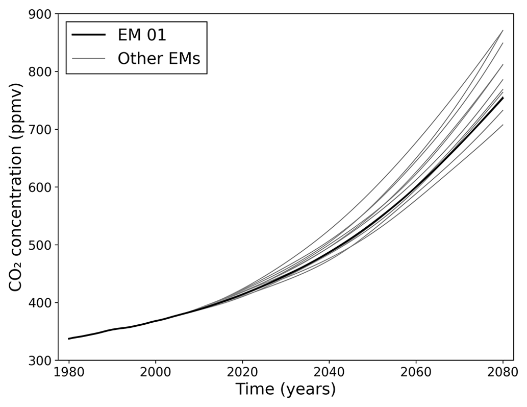
Figure 1 The global mean atmospheric CO₂ concentrations used for the UKCP18 RCM ensemble (Met Office Hadley Centre, 2020a). The heavy black line shows ensemble member 01, and the thin grey lines show the other ensemble members.

2.4 Elevation

The surface elevation data used in the calculation of HadUK-Grid were from EU-DEM v1.1 (European Environment Agency, 2021), aggregated from 25 m spatial resolution to 100 m and then linearly interpolated to the centre point of each 1 km grid box following the method used in the generation of the HadUK-Grid 1 km dataset (Hollis et al., 2019).

For the UKCP18 RCM ensemble, the climate model was run using elevation derived from EU-DEM v1.1 (European Environment Agency, 2021), smoothed appropriately for use as the lower boundary condition of the atmospheric model. After the model was run, the elevation was then regridded to the 12 km grid aligned with OSGB for distribution with the regridded climate variables (Met Office Hadley Centre, 2019) – this is the elevation used in this study.

3 Methods

Potential evapotranspiration, E_p (mm d⁻¹), was calculated using the Penman–Monteith equation (Monteith, 1965) derived in terms of specific humidity (Stewart, 1989). See Appendix A for details. The Penman–Monteith equation estimates the evaporation from an extensive vegetation-covered surface with an unlimited water supply. It has several parameters which characterise the surface, including the roughness and the stomatal resistance of transpiration, and which are dependent on the type of vegetation that is present.

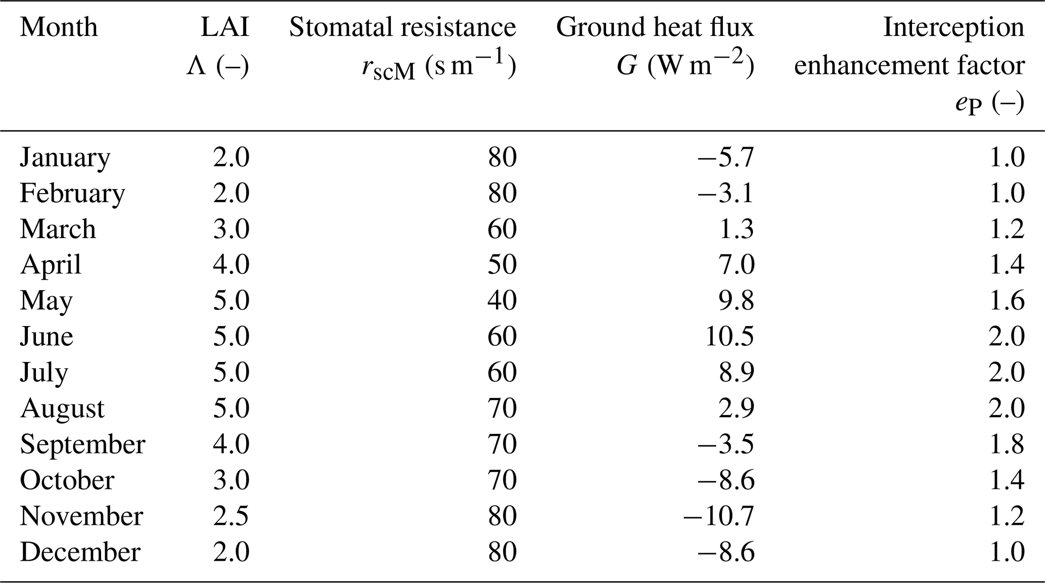
Historically, the idea of a reference crop – a hypothetical well-watered short grass – has been used for estimating PE (Allen et al., 1998). Although MORECS can be distributed for several land cover types, the most widely used for hydrological modelling in the UK is the short-grass PE (e.g. Bell et al., 2009; Rudd and Kay, 2016). This is appropriate since short grass and similar short vegetation are some of the most widespread land cover types in the UK (Morton et al., 2021). For consistency with existing hydrological modelling, we thus calculated PE for a short-grass surface. The surface parameters were chosen to match the short-grass parameterisation of MORECS v2.0; details are given in Appendix E. The grass has a canopy height of 0.12 m. The leaf area index (LAI) and stomatal resistance vary by month, and the monthly values of the parameters are given in Table 2.

Table 2 Monthly values of LAI, stomatal resistance, daily mean ground heat flux and interception enhancement factor. All values are taken from the MORECS v2.0 documentation and are valid for short grass (Hough et al., 1997).

In order to have consistent modelling from past to future, we applied the same methods to both HadUK-Grid and UKCP18 RCM meteorological data as far as possible. However, differences between the variables and temporal resolution of the two datasets engender some differences in the calculation procedures that are noted below.

The calculations were carried out with daily mean variables. This differs from MORECS v2.0, which carried out separate calculations for day-time and night-time (Hough et al., 1997). This was not possible with either the HadUK-Grid data or the UKCP18 RCM data, as they do not provide enough information about the diurnal cycle. However, tests with other datasets showed that the difference between whole-day calculations and separate day-time and night-time calculations is negligible.

3.1 Interception correction

For these datasets, we first calculated Penman–Monteith PET. We then calculated PETI by applying an interception correction on rain days. We used the methodology of MORECS v2.0, again with the parameters of a short grass to estimate the amount of rainfall which is intercepted by the canopy (Hough et al., 1997). This was done by calculating the potential interception (PEI, mm d⁻¹), which is the rate of evaporation from water intercepted by the canopy. This is subject to the same aerodynamic resistance as PET but is not limited by stomatal resistance, and so it was calculated by setting the canopy resistance r_s to zero in the Penman–Monteith equation. The PETI was calculated as a combination of PET and PEI, dependent on how much water was intercepted by the canopy each day. The interception was dependent on the amount of precipitation and the LAI. A monthly enhancement factor was applied to account for the different characteristics of rainfall in different months (see Table 2). Details of the calculations are in Appendix B.

3.2 Calculation of historical potential evaporation: Hydro-PE HadUK-Grid

The HadUK-Grid dataset does not provide exactly the variables required as input for the Penman–Monteith equation, so these were derived from the existing variables. First, all variables that were only available monthly – the sunshine hours, wind speed, vapour pressure and sea level air pressure – were interpolated to a daily time step. These were then used in combination with the existing daily variables to calculate the appropriate input variables. Details are in Appendix C, and an overview of the interpolation procedure is shown in Fig. 2.

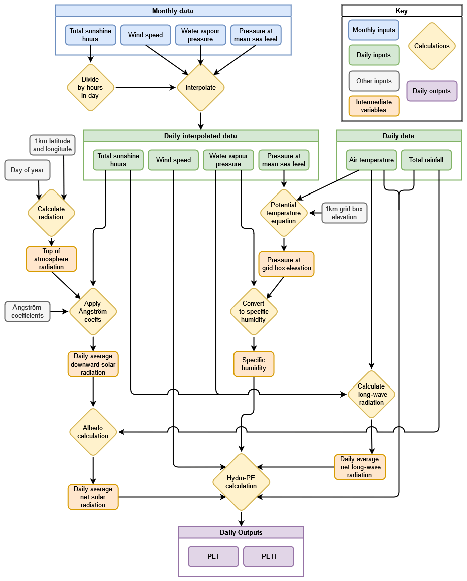
Figure 2 The temporal interpolation and calculation procedure applied to the HadUK-Grid meteorology to create daily inputs for the calculation of Hydro-PE HadUK-Grid.

Note that, since we do not have an exact estimate of net radiation from HadUK-Grid, we use a modified form of the Penman–Monteith equation that includes a correction for the radiative transfer between the surface and the screen height (Eq. A2).

3.3 Calculation of future potential evaporation: Hydro-PE UKCP18 RCM

The Penman–Monteith calculations were carried out using the daily mean values of the output from the climate model (see Appendix D). In this case, UKCP18 provides net short-wave and long-wave radiation, so the unmodified Penman–Monteith equation was used (Eq. A1). In order to account for rising levels of atmospheric CO₂, a fertilisation effect was applied to the stomatal resistance following the method of Kruijt et al. (2008) (see Appendix E5 for details).

Since the UKCP18 output is provided for all land and sea points in the domain but PET and PETI are only valid over land, we only carried out the calculations for land points. The land points were selected using the land–sea mask provided by the Met Office (Met Office Hadley Centre, 2020b), which defines grid boxes as either 100 % sea or 100 % land. There are some grid boxes which, although they are classified as sea in the RCM, do actually contain a small fraction of land. This is particularly important for hydrological models which run by disaggregating the meteorological inputs to a higher spatial resolution for calculating river flows. In order to allow the PET and PETI to be used as input to such hydrological models, these grid boxes were filled with valid data. To do this, a mapping was created between each grid box which needed to be filled and the nearest comparable land grid box. Then the PET and PETI were copied from the existing land grid boxes to the target grid boxes. This was done rather than calculating the PET and PETI with the existing meteorology in the RCM output, because the meteorology over the sea would be unrepresentative of land.

4 Results

Maps of Hydro-PE HadUK-Grid PET and PETI can be seen in Fig. 3. There is a strong north-west to south-east gradient, with low values in the west of Scotland and high values in south-eastern England, which follows the climate of the regions from colder and wetter in the north-west to warmer and dryer in the south-east. Maps of Hydro-PE UKCP18 RCM PET and PETI can be seen in Figs. 4 and 5 respectively. Each panel shows the overall mean PET and PETI for each ensemble member. While there is a range across the ensemble, reflecting the range in ensemble meteorology, there is a consistent spatial pattern across the ensemble, which is also consistent with the HadUK-Grid PET and PETI maps (Fig. 3).

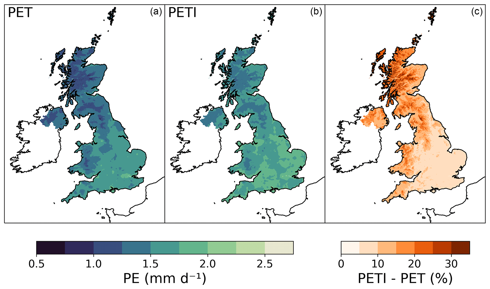
Figure 3 Annual mean PET (a) and PETI (b) from Hydro-PE HadUK-Grid (1969–2021). Panel (c) shows the relative difference between PETI and PET as a percentage of PET.

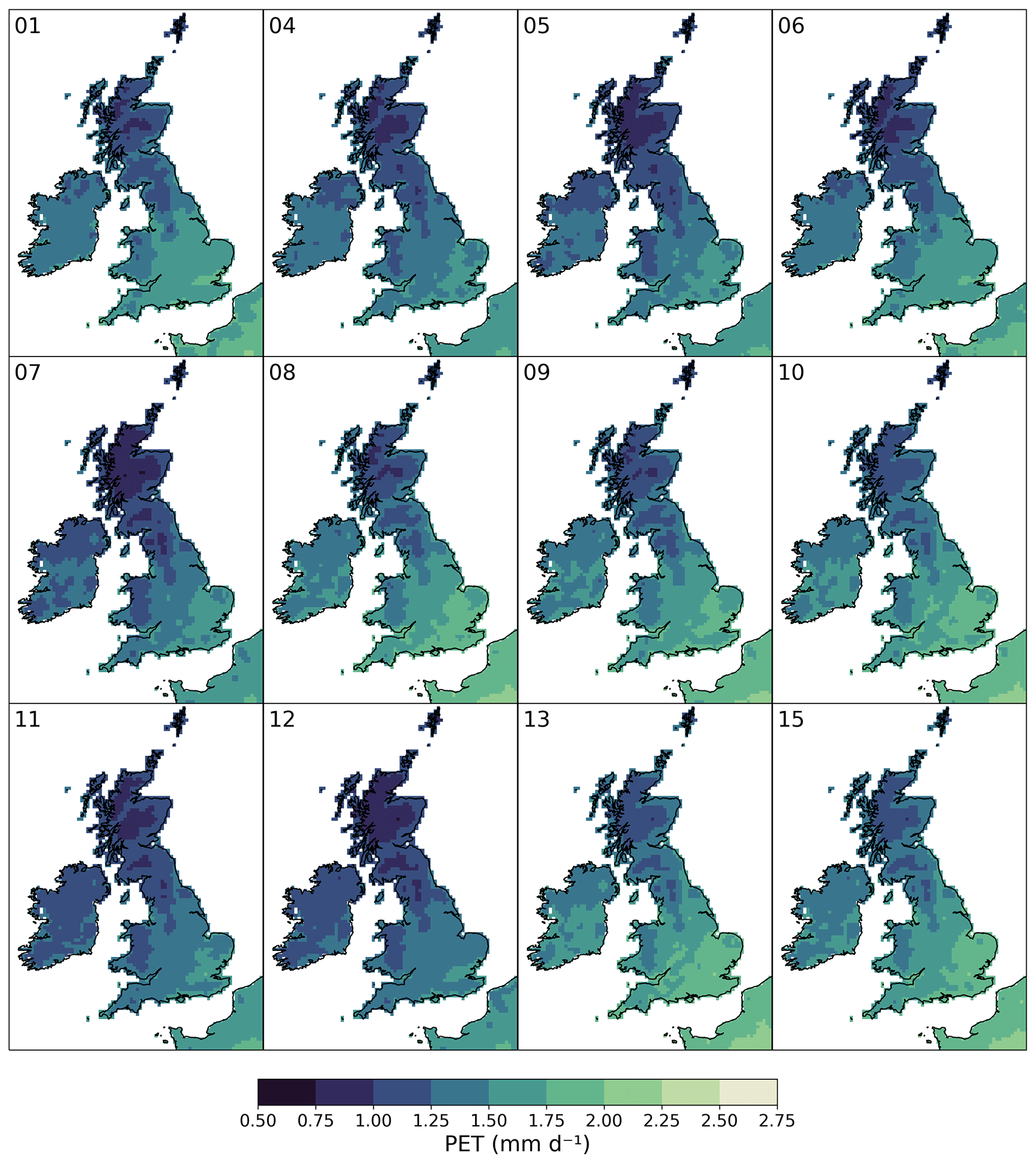
Figure 4 Mean PET for each ensemble member of Hydro-PE UKCP18 RCM over the historical period 1980–2020.

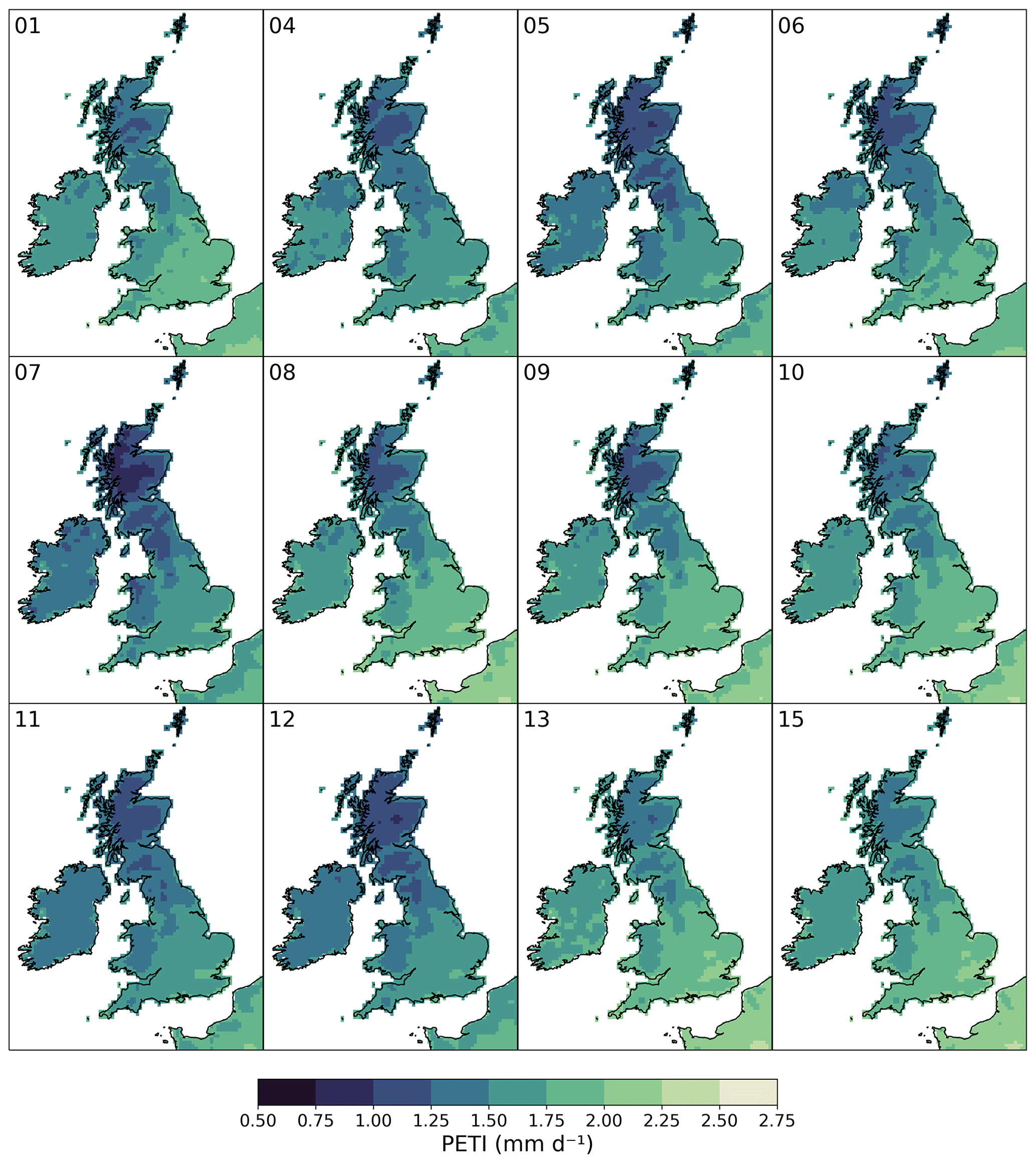
Figure 5 Mean PETI for each ensemble member of Hydro-PE UKCP18 RCM over the historical period 1980–2020.

Time series of annual mean PET and PETI are shown in Fig. 6 for Hydro-PE HadUK-Grid and the Hydro-PE UKCP18 RCM ensemble. The mean monthly climatologies of PET and PETI are shown in Fig. 7 for the first 20 years of the UKCP18 RCM ensemble (1980–2000) and the last 20 years (2060–2080). The Hydro-PE UKCP18 RCM ensemble is consistent with Hydro-PE HadUK-Grid in the historical period, although Hydro-PE HadUK-Grid has an increase in PET and PETI in May followed by a levelling off in June that is not seen in Hydro-PE UKCP18 RCM. This is due to differences in the seasonality of the input meteorology (see Sect. 5). Overall, both PET and PETI increase over the course of the future projections, with PET increasing by 16 %–29 % and PETI increasing by 14 %–25 %. The largest increases are in the summer (21 %–36 % for PET and 18 %–30 % for PETI). Increases are more moderate in the winter, and some ensemble members individually show a decrease in PET and PETI for the winter months.

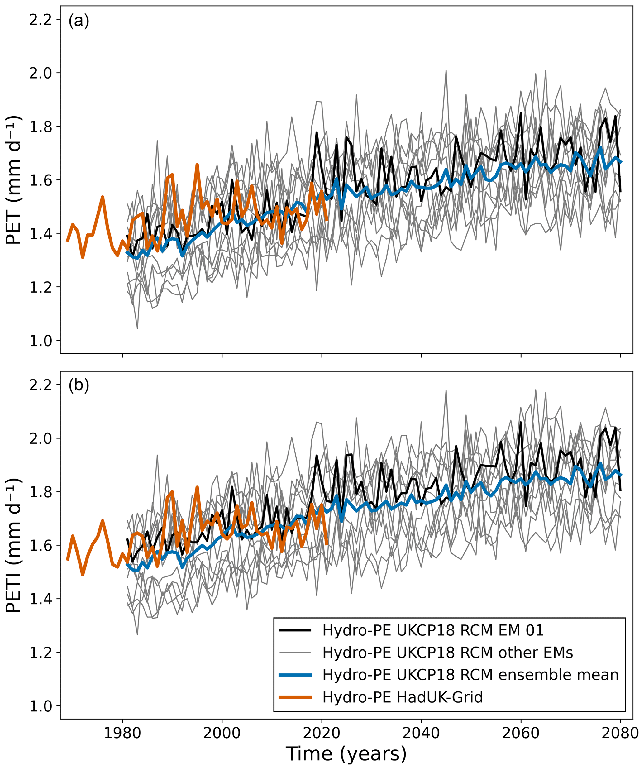
Figure 6 Time series of annual mean PET (a) and PETI (b). The black line shows ensemble member 01 of Hydro-PE UKCP18 RCM, the grey lines show the other ensemble members, and the blue line shows the ensemble mean. The orange line shows Hydro-PE HadUK-Grid. Note that the regions averaged are slightly different – Hydro-PE UKCP18 RCM averages over the UK, the Republic of Ireland, and a small area of northern France, while Hydro-PE HadUK-Grid only includes the UK.

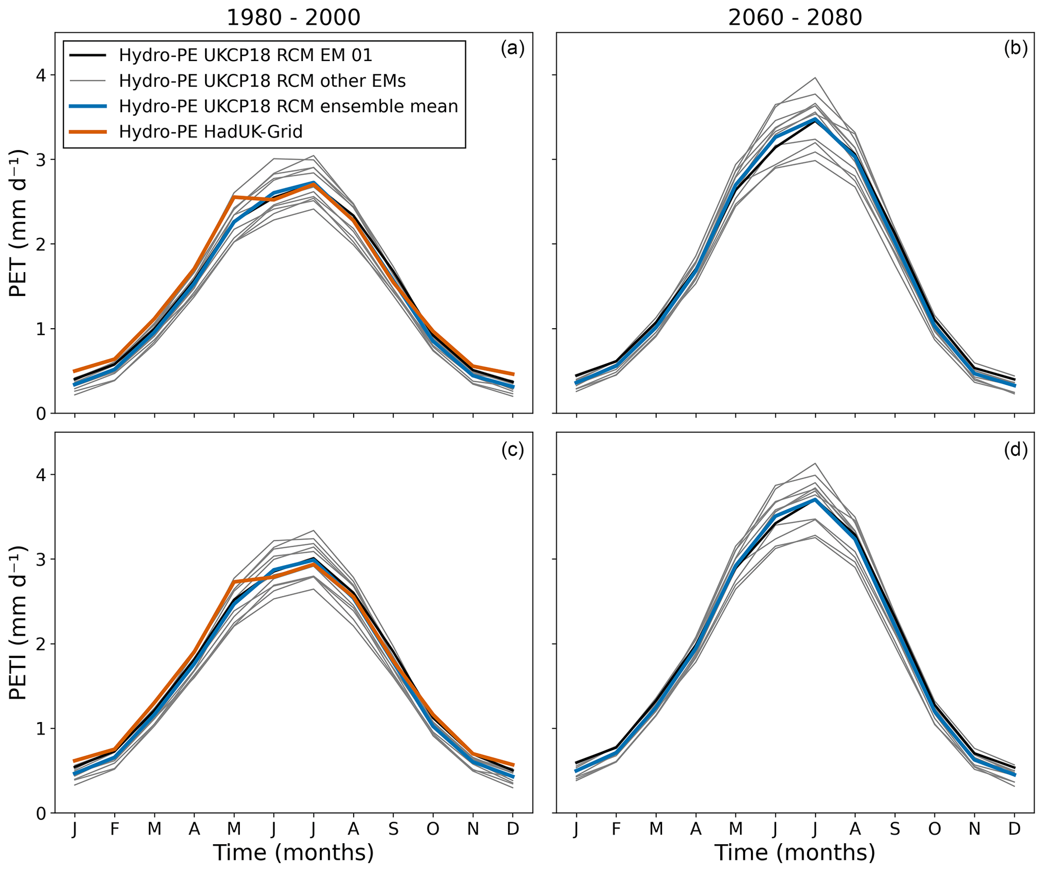
Figure 7 Mean monthly climatology of PET (a, b) and PETI (c, d). Panels (a) and (c) show the mean over the first 20 years of the ensemble. Panels (b) and (d) show the mean over the final 20 years. Line styles as in Fig. 6.

Maps of the difference between PETI and PET (as a percentage of PET) are shown in Fig. 8 for Hydro-PE UKCP18 RCM and in Fig. 3c for Hydro-PE HadUK-Grid. The effect of including interception increases the PE estimate by 5 %–10 % in low-lying areas of south-eastern England but has a larger increase of up to 35 % in the Highlands of Scotland. This is because the latter have a relatively low evaporative demand (because they are cooler and wetter than other regions) but larger amounts of rainfall than the rest of the country.

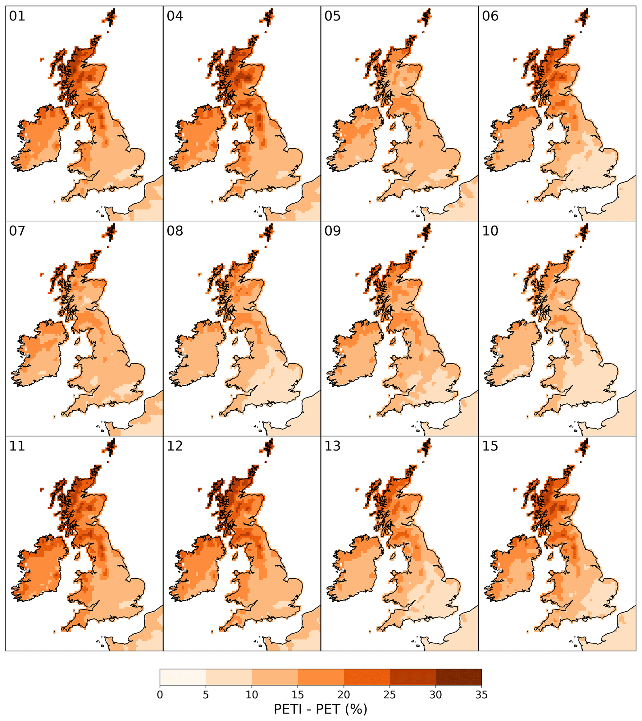
Figure 8 The difference between annual mean PETI and annual mean PET as a percentage of PET for each ensemble member over the historical period of Hydro-PE UKCP18 RCM (1980–2020).

The mean monthly climatology of the difference between PETI and PET can be seen in Fig. 9. The mean value of the interception correction is largest in the summer months (0.21–0.32 mm d⁻¹) and lowest in the winter months (0.10–0.14 mm d⁻¹) in the historical period of Hydro-PE UKCP18 RCM, although as the overall PET is lower in the winter, this leads to a larger relative difference in the winter than in the summer. This is consistent with Hydro-PE HadUK-Grid, which has mean interception corrections of 0.23–0.27 mm d⁻¹ for the summer months and 0.11–0.12 mm d⁻¹ for the winter months.

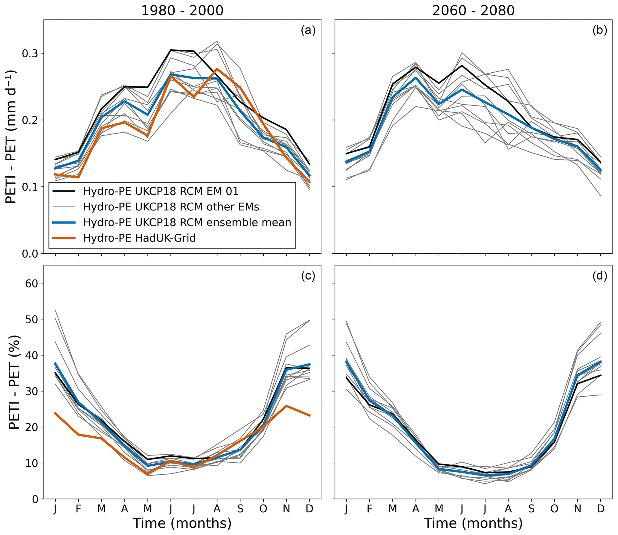
Figure 9 Mean monthly climatology of the difference between PETI and PET as an absolute value (a, b) and as a percentage of PET (c, d). Panels (a) and (c) show the mean over 1980–2000. Panels (b) and (d) show the mean over 2060–2080. Line styles as in Fig. 6.

In the future, the interception correction decreases in the summer months by 14 % (to 0.16–0.30 mm d⁻¹) and increases in the winter by 8 % (to 0.08–0.18 mm d⁻¹), leading to little change at the annual scale. The decrease in summer interception correction is why the relative increase in PETI is smaller than that of PET. The peak in the absolute difference between PETI and PET is shifted to earlier in the year (from June–September in the historical period to March–June at the end of the projections). This may contribute to the changing seasonality of river flows under future climates.

The Hydro-PE UKCP18 RCM interception correction is consistent with the Hydro-PE HadUK-Grid interception correction throughout the year. However, the ensemble mean is higher than Hydro-PE HadUK-Grid for most of the year but is lower in autumn. This is consistent with the model biases in the precipitation, as the model simulations overall have a higher precipitation than HadUK-Grid for most of the year but a slightly lower precipitation from August to October (Fig. 10).

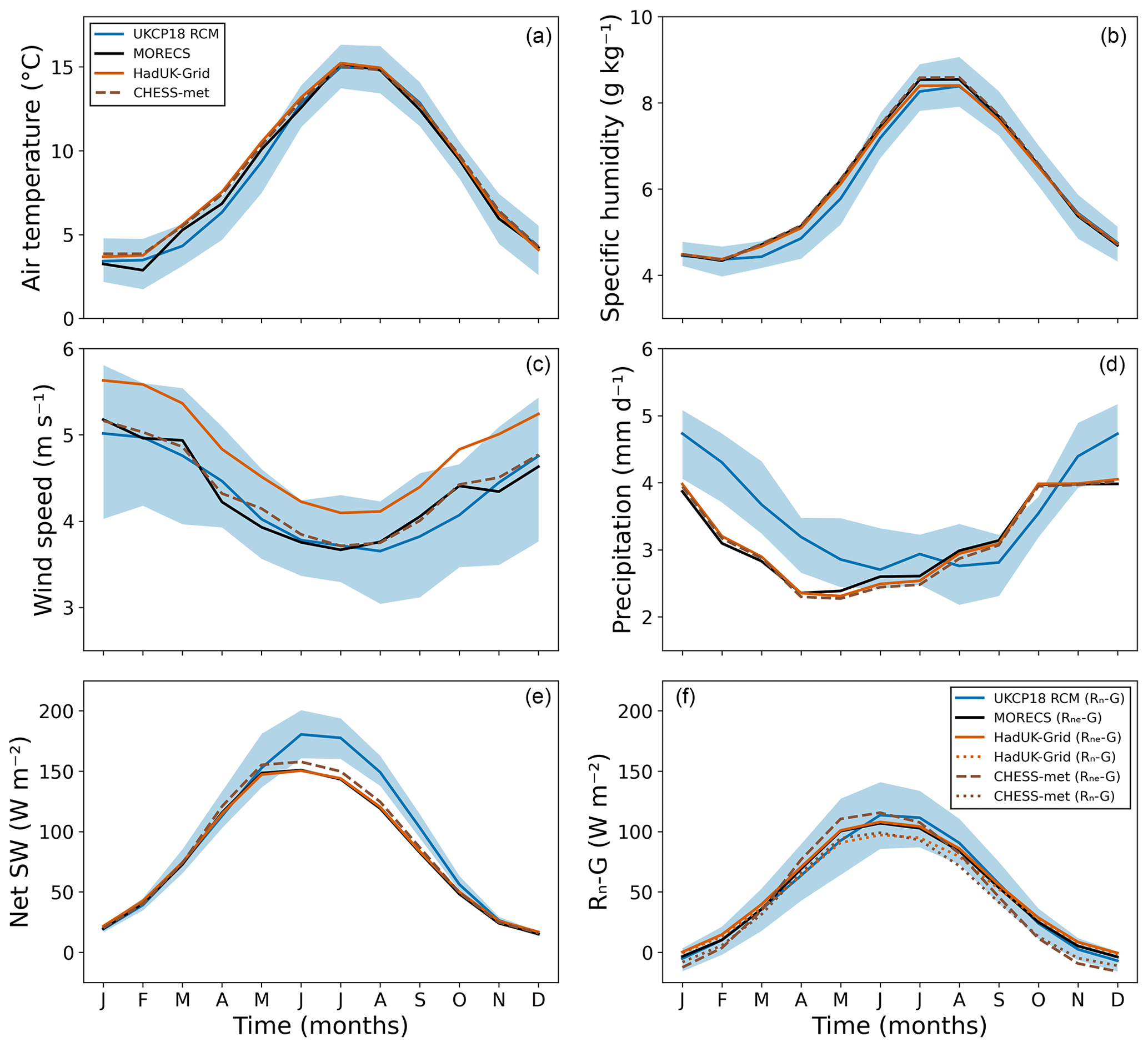
Figure 10 Monthly mean air temperature (a), specific humidity (b), wind speed (c), precipitation (d), net short-wave radiation (e) and available energy (f) averaged over GB (1981–2017) for MORECS (black line), UKCP18 RCM (blue line shows the ensemble mean and light-blue area shows the ensemble range), HadUK-Grid (orange line) and CHESS-met (brown dashed line). The MORECS specific humidity, short-wave radiation and available energy have been calculated from the daily MORECS meteorology, so they are an approximation of the full day- and night-time calculations. In panel (f), the MORECS, HadUK-Grid and CHESS-met lines show the available energy used in the PE calculations, which was calculated using the approximate long-wave radiation R_ne, which assumes the surface temperature can be approximated with the air temperature (Eq. C12). The dotted orange and brown lines show the available energy with an estimate of the correction from Eq. (A3) applied and so are comparable with the UKCP18 RCM values, which are calculated using the actual net radiation components outputted by the climate model.

Both variables show an increasing trend in the mean through the historical period and climate projections. The future projections of PET and PETI both increase by 0.29 mm d⁻¹ overall between 1980–2000 and 2060–2080, which is 22 % of PET and 19 % of PETI. The increase varies across the ensemble between 0.23 and 0.38 mm d⁻¹. The relative increase ranges between 16 % and 29 % of PET and between 15 % and 25 % of PETI. However, there is little change in the winter values (<0.1 mm d⁻¹), but in the summer both PET and PETI increase by around 0.7 mm d⁻¹ overall (ranging between 0.5 and 1.0 mm d⁻¹ across the ensemble).

The 90th percentile values for each month in Hydro-PE HadUK-Grid and Hydro-PE UKCP18 RCM are shown in Fig. 11. The Hydro-PE UKCP18 RCM ensemble is consistent with Hydro-PE HadUK-Grid between June and September, but for the rest of the year the Hydro-PE HadUK-Grid 90th percentile is higher than Hydro-PE UKCP18 RCM. This is an artefact of using smoothly interpolated HadUK-Grid inputs in the calculations applied to obtain the input variables (Appendix C), causing the 90th percentiles in Hydro-PE HadUK-Grid to be high rather than causing Hydro-PE UKCP18 RCM to be too low (see Sect. 5.1 and 5.4 for further discussion of this).

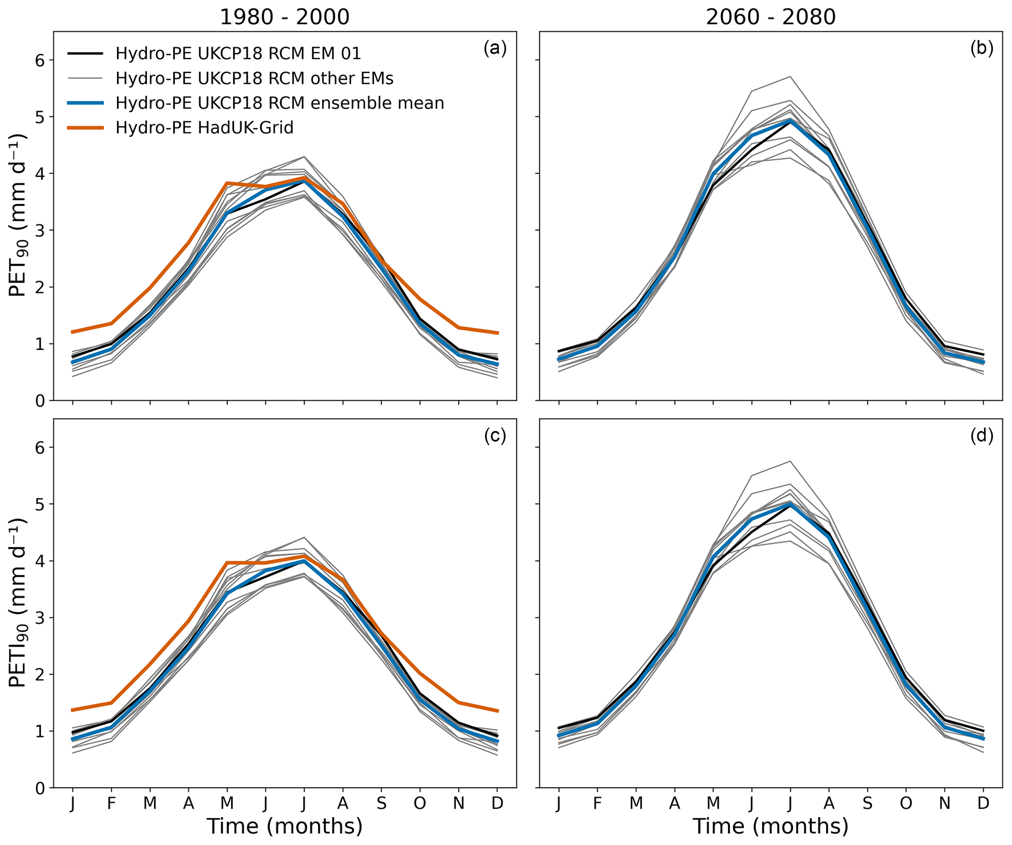
Figure 11 Monthly 90th percentiles of PET (a, b) and PETI (c, d). Panels (a) and (c) show the percentiles calculated over the first 20 years of the ensemble. Panels (b) and (d) show them calculated over the final 20 years. Line styles as in Fig. 6.

Similarly to the mean, there is little change in the Hydro-PE UKCP18 RCM 90th percentile values in winter, with some ensemble members showing a small decrease (up to −0.10 mm d⁻¹ for both PET₉₀ and PETI₉₀) and some a small increase (up to 0.17 mm d⁻¹ for both PET₉₀ and PETI₉₀). The increases in the 90th percentiles in the summer are much larger and are larger than the increase in the mean, with PET₉₀ increasing between 0.50 and 1.54 mm d⁻¹ and PETI₉₀ increasing between 0.47 and 1.47 mm d⁻¹.

The increases in mean PET and PETI and in the 90th percentiles are driven by increasing temperature, decreasing relative humidity and increasing solar radiation (due to decreasing cloud cover) in the climate projections (Murphy et al., 2018). Increases in PETI are mitigated by projected decreases in rainfall in the summer (Murphy et al., 2018), so that the relative contribution of the interception correction falls from 10 % of summer PET (14 % of annual PET) to 7 % of summer PET (12 % of annual PET) by the end of the projections.

5 Evaluation

5.1 Comparison with spatial PE datasets across Great Britain

As the Hydro-PE method has been designed to calculate PETI to be comparable with MORECS PE for short grass, we have compared Hydro-PE HadUK-Grid and Hydro-PE UKCP18 RCM with MORECS. We have also compared it with the existing CHESS-PE PET and PETI datasets. We have calculated mean monthly climatologies for the common period 1981–2017 and for Great Britain (GB) only, as this is the land area that is common to all four datasets. These can all be seen in Fig. 12. Both Hydro-PE HadUK-Grid PET and the ensemble mean of Hydro-PE UKCP18 RCM PET are lower than MORECS PE, which is as expected (because of the inclusion of the interception correction in MORECS), but Hydro-PE UKCP18 RCM PETI is higher than MORECS PE in the summer and Hydro-PE HadUK-Grid PETI is higher than MORECS throughout the year. CHESS-PE PET and PETI are both lower than MORECS due to differences in the PE calculations and parameterisations. (The related FAO reference crop evaporation (Pereira et al., 1999) is a PET calculation that does not consider interception, so it will give a low estimate of PE when used for hydrology compared to PETI.) The 90th percentiles calculated over 1980–2000 for GB are in Fig. 13. The Hydro-PE UKCP18 RCM values are consistent with CHESS-PE throughout the year, while the Hydro-PE HadUK-Grid 90th percentiles are higher than CHESS-PE, particularly between October and April. This is due to the temporal interpolation from monthly to daily combined with the assumptions used to calculate the required inputs from the available HadUK-Grid variables (Appendix C). This is further discussed in Sect. 5.4.

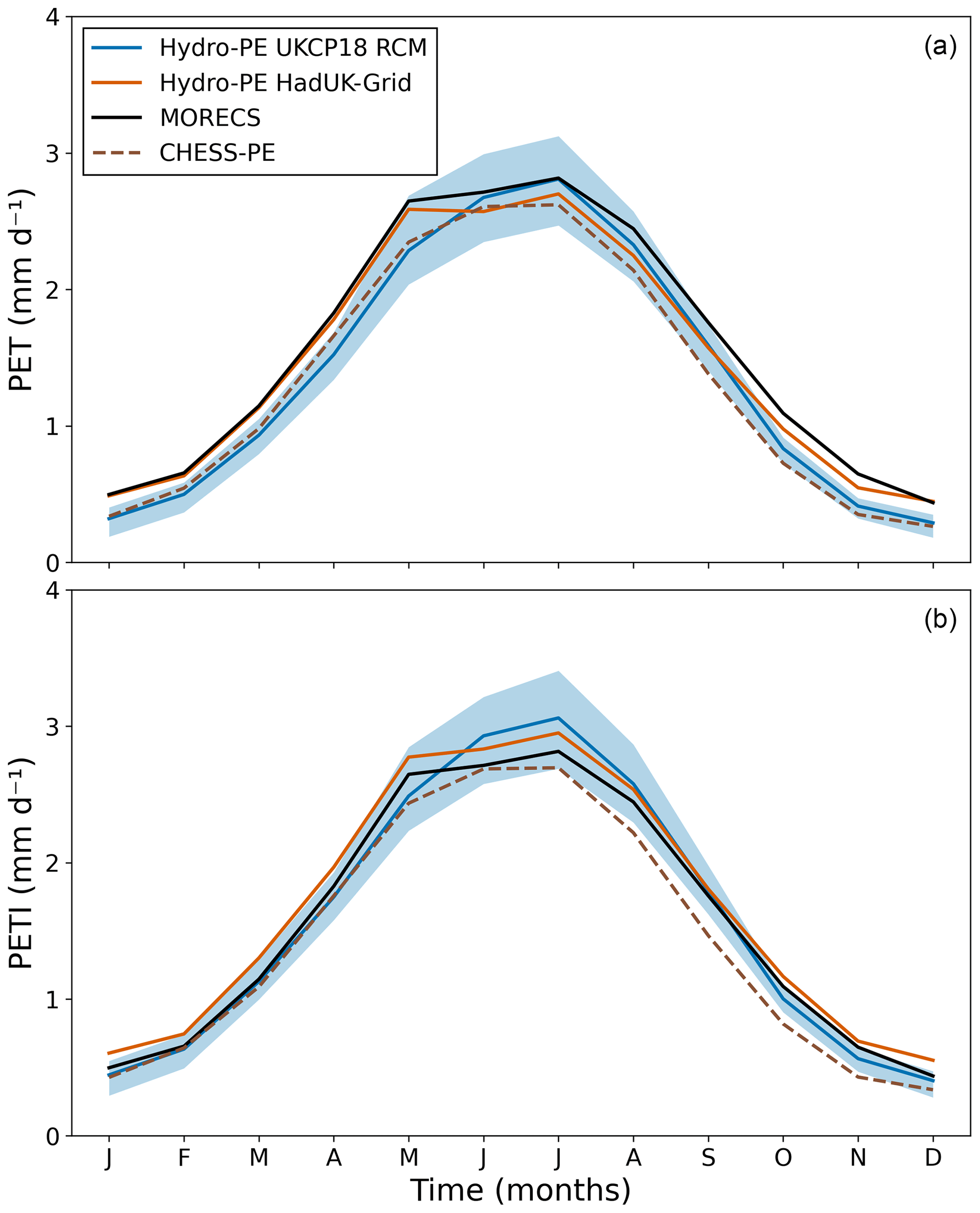
Figure 12 Monthly mean PET (a) and PETI (b) averaged over GB for 1981–2017. The black line in both panels is MORECS PE (which includes the interception correction and so is equivalent to PETI). The blue line shows the ensemble mean of Hydro-PE UKCP18 RCM, and the light-blue area shows the ensemble range. The orange line shows Hydro-PE HadUK-Grid. The brown dashed line shows CHESS-PE.

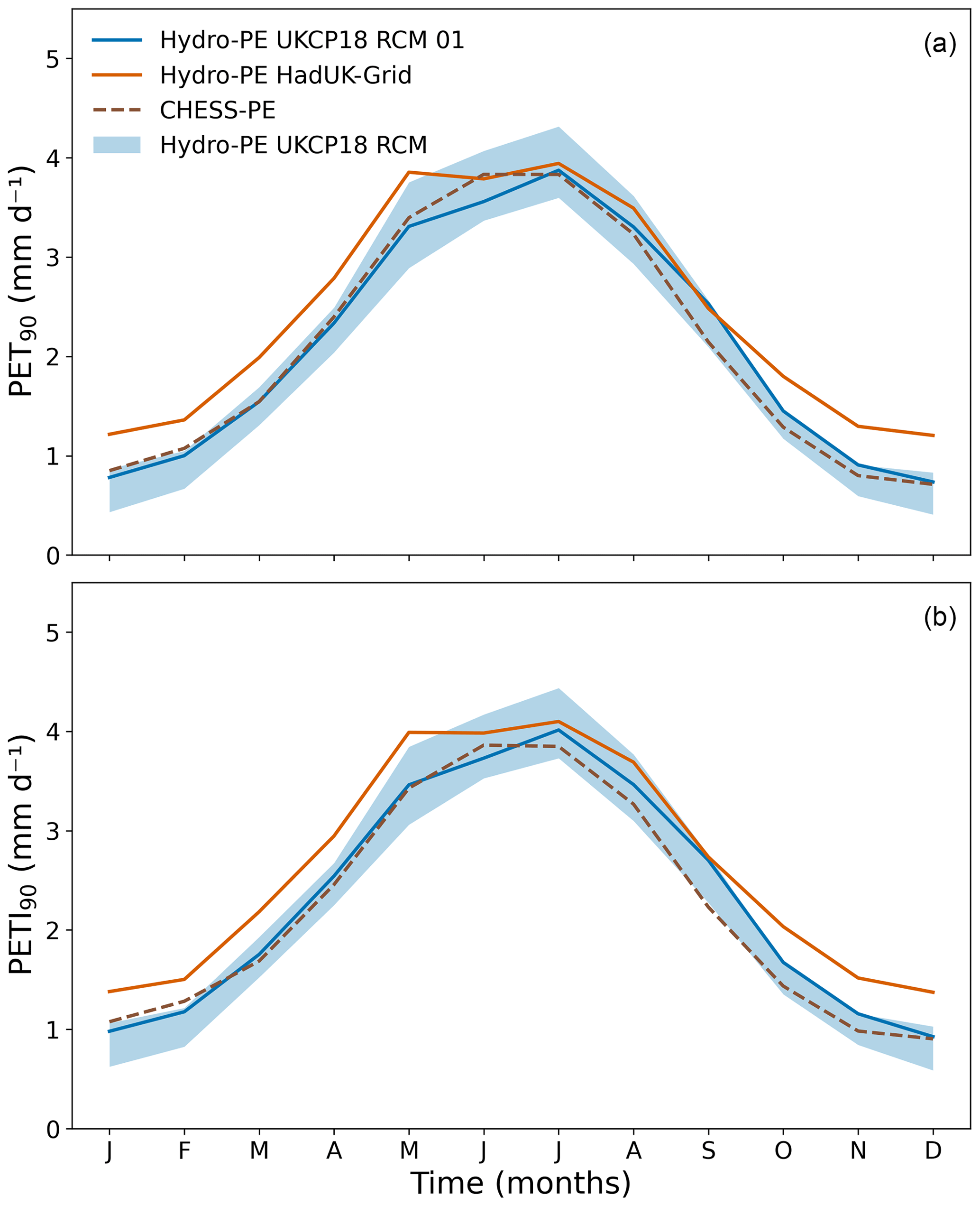
Figure 13 Monthly 90th percentile of PET (a) and PETI (b) averaged over GB for 1981–2000. The blue area shows the ensemble range of Hydro-PE UKCP18 RCM, and the black line shows the values for ensemble member 01. The orange line shows Hydro-PE HadUK-Grid. The brown dashed line shows CHESS-PE.

The differences between the four datasets are due to either (a) differences in the input meteorology or (b) differences in the methodology. Since CHESS-met is derived from MORECS meteorology, we expect the differences between MORECS PE and CHESS-PE PETI to be due to methodological differences. However, since we have developed the Hydro-PE methodology to be as similar to MORECS as possible, the differences between Hydro-PE and MORECS PE should be due to differences between the meteorology in MORECS, HadUK-Grid and UKCP18 RCM, including differences in the calculation of the input variables from the available data.

Since HadUK-Grid and MORECS meteorology are derived from the same network of station observations (although not exactly the same stations) and CHESS-met is derived directly from MORECS, we might expect the meteorology averaged over a region to be very similar in all three datasets. Indeed, there is good agreement in GB mean air temperature and precipitation between HadUK-Grid, MORECS and CHESS-met (Fig. 10), although MORECS air temperature is a little lower in the winter and MORECS precipitation is a little higher in the summer – this is likely due to the slightly different spatial coverage of the different resolutions. However, the different methods of downscaling of some variables from stations or MORECS to the 1 km grid can introduce differences between datasets. Most notably, the GB mean HadUK-Grid wind speeds are much higher than all of the other datasets. This is due to very high wind speeds at high elevations in HadUK-Grid, particularly in Scotland, due to the elevation adjustment used in the HadUK-Grid calculations (Hollis et al., 2019). Figure 14 shows that, in Scotland, the HadUK-Grid wind speeds are much higher than the other observational datasets, while in England they are all comparable. Since MORECS is representative of a hypothetical site at mean grid box elevation (rather than mean grid box meteorology) and has a lower resolution, it does not represent these high wind speeds. The CHESS wind speed corrections were applied to the MORECS wind speed assuming that it does represent mean grid box wind speed, so the CHESS corrections are also not able to reproduce high wind speeds. The HadUK-Grid wind speeds were adjusted based on topographic relationships without assuming a preservation of the mean (Hollis et al., 2019). The high values of Hydro-PE HadUK-Grid are likely more representative of high elevations.

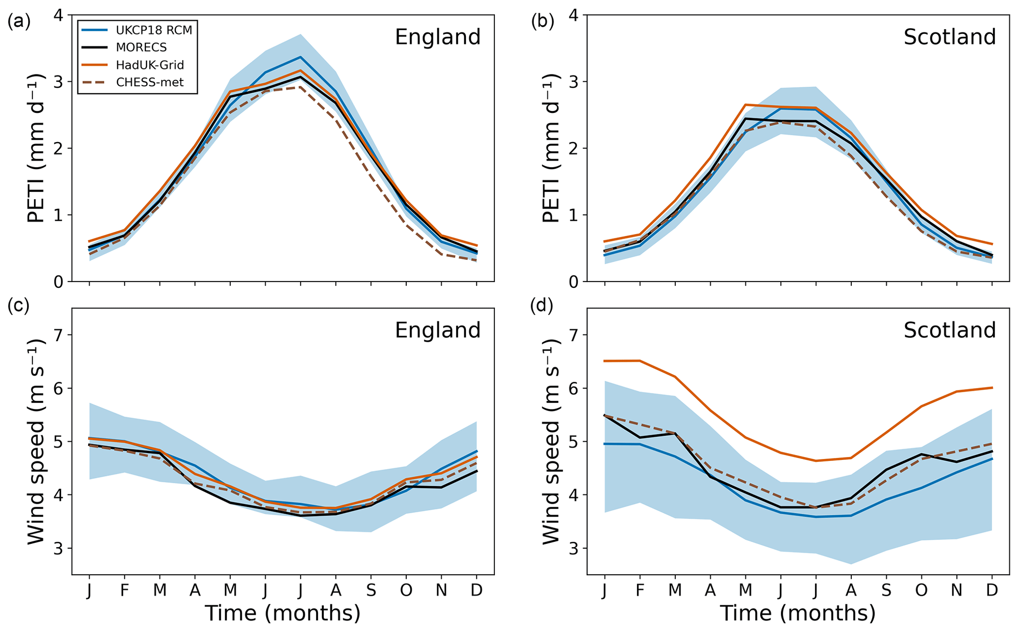
Figure 14 Monthly mean PETI (a, b) and wind speed (c, d) averaged over England (a, c) and Scotland (b, d) (1981–2017) from MORECS (black line), UKCP18 RCM (blue line shows the ensemble mean and light-blue area shows the ensemble range), HadUK-Grid (orange line) and CHESS (brown dashed line).

Other variables that are used in the calculation of PE are not directly observed but have been derived from the variables provided by the station observations. There are differences in the methodology between HadUK-Grid, MORECS and CHESS that lead to some differences in inputs to the PE calculations (Fig. 10). The specific humidity of HadUK-Grid is lower than MORECS in the summer, which leads to a higher humidity deficit (as the air temperature is nearly the same). The net short-wave radiation is very similar between HadUK-Grid and MORECS, as they are both calculated using the same methodology. CHESS-met uses the same method to calculate downward short-wave radiation but adjusts for slope and aspect, and it uses a different albedo parameterisation, so the CHESS-met net short wave is slightly higher. The approximate total available energy (calculated with R_ne, Eq. C8) calculated from HadUK-Grid is very similar to that calculated from MORECS meteorology. In CHESS-met the approximate available energy is higher because the net radiation is calculated differently and because CHESS does not include a ground heat flux. Overall, it is the combination of the higher wind speed and lower specific humidity in HadUK-Grid that leads to the higher PETI in Hydro-PE HadUK-Grid than in MORECS.

In addition to the differences in the means, the differences in methodologies have also had an impact on the extremes of the datasets. In particular, the Hydro-PE HadUK-Grid 90th percentiles are relatively high due to a combination of the radiation calculations (Sect. 5.4) and the temporal interpolation of the monthly input variables. The CHESS-PE 90th percentiles are also relatively high compared to the mean values in winter, which is likely to also be due to the use of the same short-wave radiation calculation, but the effect is not as large as for Hydro-PE HadUK-Grid, as the CHESS input variables are all daily. It was not possible to investigate the MORECS percentiles, as MORECS was only available as monthly means.

The UKCP18 variables have been obtained from a free-running climate model that has not had any bias-correction applied. This means that although the climate model has been calibrated and parameterised against historical meteorological data, it is not expected to match the observed climate exactly. This may be down to deficiencies in the model structure and/or calibration but is also due to large-scale climate variability. The UKCP18 RCM reproduces the historical air temperature well, although the ensemble is slightly cooler than the observations in the spring (Fig. 10). However, it significantly overestimates precipitation through most of the year compared to MORECS and slightly underestimates precipitation from August to October. This is likely due to the global circulation in the coarser-resolution GCM within which the RCM is nested bringing more moisture to western Europe (Murphy et al., 2018). This results in a larger interception correction than is seen in the historical Hydro-PE HadUK-Grid for much of the year.

Again, the UKCP18 RCM has a lower specific humidity than MORECS (Fig. 10), which in the spring and summer leads to a higher humidity deficit. The wind speed is very similar between the climate model and the observations, but the net short-wave radiation is much higher in the summer and autumn in the climate model. This is likely to be due to a lower amount of cloud in the model and partly due to different albedo values. In particular, the climate model is run with a realistic land cover, while the net short-wave radiation is calculated for all the other PE datasets assuming short grass everywhere. Overall, the available energy (calculated with the actual net radiation R_n, Eq. D1) calculated with UKCEP18 RCM is higher than that calculated with either HadUK-Grid or CHESS-met. It cannot be compared to MORECS because we do not have actual net radiation for MORECS, but since we can see that MORECS and HadUK-Grid have very similar approximate available energies, R_ne, we can infer that the UKCP18 RCM actual available energy is also higher than MORECS. Therefore, the high values of Hydro-PE UKCP18 RCM PETI in the summer are likely to be due to a combination of lower humidity and much higher available energy than in MORECS. The fact that the high May values of PETI seen in Hydro-PE HadUK-Grid and MORECS are not seen in Hydro-PE UKCP18 RCM is due to the seasonal cycle of temperature, humidity and available energy being shifted later in the year in the climate model than in the observations.

So, although there are differences between the Hydro-PE products and MORECS in the historical period, these are due to understood differences in the input meteorology.

5.2 Comparison with daily MORECS site data

The Hydro-PE HadUK-Grid PETI data were further compared to daily MORECS PE data for 16 sites across GB available for the period 1 January 1985–31 December 1992. The MORECS PE data are derived from observed station data at each site. These are compared with the HadUK-Grid PETI from the 1 km grid box that contains each site (see Table 3). We expect some differences between the MORECS PE and the Hydro-PE HadUK-Grid PETI due to the difference in location, and therefore meteorology, between the MORECS sites and the HadUK-Grid 1 km grid box centres.

Three metrics were calculated to evaluate daily Hydro-PE HadUK-Grid PE relative to daily MORECS PE: (a) bias calculated as the difference in mean daily PE values annually and seasonally, (b) difference in the standard deviation in daily PE and (c) Pearson correlation coefficient of daily PE values and of deseasonalised daily PE values. The results are presented in Fig. 15, with boxplots summarising results over the 16 sites (Fig. 15a–c) and maps showing results at the site locations (Fig. 15d–f).

Table 3 Sites used for evaluation, together with the corresponding HadUK-Grid grid boxes. The top section gives details for MORECS sites, and the bottom section gives details for the eddy covariance sites. Locations are given in British National Grid coordinates, with HadUK-Grid locations and elevations referring to the centre of the selected grid box. Distance (m) and elevation difference (m) refer to the difference in location and elevation between the sites and the centre point of the HadUK-Grid grid box.

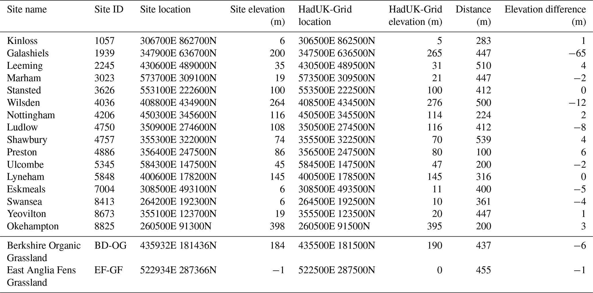
Figure 15 Evaluation of the Hydro-PE HadUK-Grid PETI against daily MORECS PE (which is also PETI) across 16 MORECS sites. Boxplots summarise results over all 16 sites, including (a) bias in mean daily PETI values calculated annually (Ann) over winter (DJF), spring (MAM), summer (JJA) and autumn (SON); (b) difference in the standard deviation of daily values; and (c) Pearson correlation coefficient for the raw daily values (black) and the deseasonalised daily values (grey). Maps show annual bias, difference in the standard deviation and Pearson correlation coefficient values for the raw daily data at each of the MORECS sites.

The HadUK-Grid PETI is higher throughout the year than MORECS PE, as shown by the positive biases across all the sites and seasons (Fig. 15a and d). This echoes the results from the GB-wide comparison in Fig. 12. HadUK-Grid PETI also tends to have slightly higher variation than MORECS PE, as shown by a higher standard deviation in PE time series for 9 out of the 16 sites. Correlation between HadUK-Grid PETI and MORECS PE is generally good across all the sites, with Pearson correlation coefficients in the range 0.72–0.81. The high Pearson correlation coefficients are partly due to the fact that we represent the seasonal cycle well. With deseasonalised data, the Pearson correlation coefficients are in the range 0.30–0.47, which still shows a reasonable correlation with the MORECS PE. Even though the need for temporal interpolation of some HadUK-Grid variables from monthly to daily is likely to suppress the daily variability to some extent, the daily variability of the calculated PETI is still comparable to observations.

5.3 Comparison with eddy covariance measurements

While PET and PETI are not directly observable quantities, they are an estimate of unconstrained evapotranspiration. In GB in the winter, spring and autumn evaporation rates are low and precipitation is high, so it can be assumed that most evaporation will occur at the potential rate. Thus we can compare eddy covariance (EC) flux measurements of actual evaporation (AE, mm d⁻¹) with PETI calculated from the meteorological measurements at each EC site using the Hydro-PE methodology (EC site PETI). We also compare this with the Hydro-PE HadUK-Grid PETI from the 1 km grid box containing each site with the EC site PETI.

We used measurements of AE and meteorology from two EC sites in England.

Berkshire Organic Grassland (BD-OG)

This site is located on an organically managed grassland in the Berkshire downs at an elevation of 184 m above sea level (Evans et al., 2016b). EC measurements are available from 1 January 2017 to 16 November 2019 (Morrison et al., 2019).

East Anglia Fens Grassland (EF-GF)

This site is located on a managed grassland in a lowland peatland environment in the East Anglian Fens at an elevation of 1 m below sea level (Evans et al., 2016a). EC measurements are available from 27 April 2017 to 31 March 2019 (Morrison et al., 2020).

Details of the site locations and the corresponding HadUK-Grid 1 km grid boxes are shown in Table 3.

Figure 16a and b show the time series of EC site PETI and the measured AE. The PETI is similar to the AE, except in the summer (JJA), when the AE drops below the PETI due to soil moisture limitation. Figure 17a and b show the EC site PETI plotted against the measured AE (excluding JJA values) at each site. There is a near-one-to-one linear fit between the PETI and the AE at both sites, although there is a small negative bias that may be due to differences between the sites and the idealised short grass used for the PETI parameterisation. In particular, EG-GF is sited on peat soils, which are not accounted for in the parameterisation. The difference in the standard deviation is also small. The Pearson correlation is very high, at 0.92 for BD-OG and at 0.90 for EF-GF. Thus it can be concluded that, at the EC sites, the PETI calculated with observed meteorology is representative of the observed AE during times of no water stress.

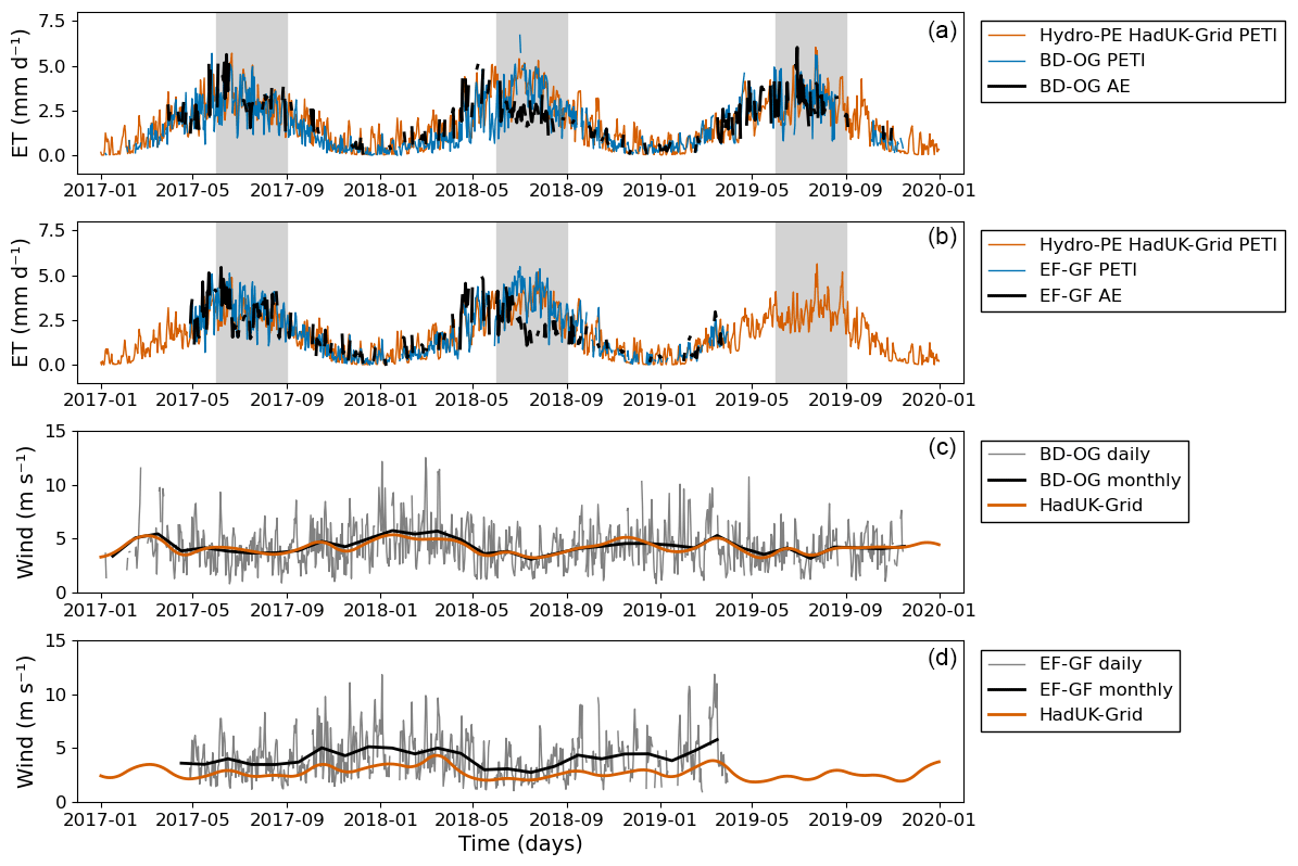
Figure 16 Panels (a) and (b) show time series of measured daily AE (black), calculated daily PETI (blue) and HadUK-Grid PETI (orange) for two EC sites (BD-OG and EF-GF). The grey regions show the summer data that are excluded from calculating the metrics. Panels (c) and (d) show observed daily wind speed (grey), observed monthly mean wind speed (black) and HadUK-Grid-interpolated wind speed (orange) for the two EC sites.

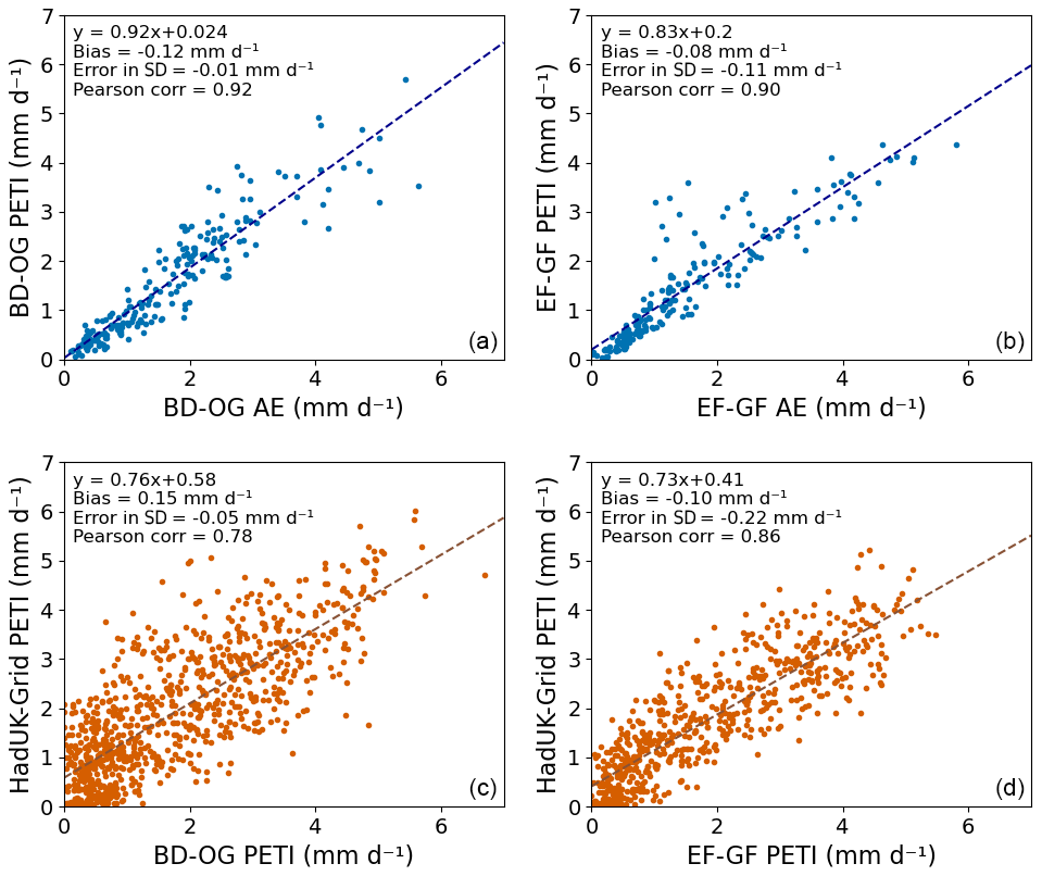
Figure 17 Panels (a) and (b) show PETI calculated from site meteorology plotted against observed AE for values in winter (DJF), spring (MAM) and autumn (SON). Panels (c) and (d) show the HadUK-Grid PETI against the EC site PETI. Panels (a) and (c) are the BD-OG site, and panels (b) and (d) are the EF-GF site. Dashed lines show the least-squares linear fit to the data.

Figure 16a and b also show the time series of Hydro-PE HadUK-Grid PETI from the grid box that contains each EC site. The HadUK-Grid PETI compares well with the EC site PETI (Fig. 17c and d), with Pearson correlations of 0.78 and 0.86, similar to the comparison with daily MORECS site PE. For BD-OG there is a small positive bias, while for EG-GF there is a small negative bias. The latter is likely due to the low wind speed in HadUK-Grid compared to the wind speed observed at the EC site (Fig. 16d). There may also be an effect of the peat soil that is not represented by the MORECS parameterisation.

The standard deviation of the Hydro-PE HadUK-Grid PETI is lower than the standard deviation of the EC site PETI, but the difference is small. There is a lack of daily variability in the temporally interpolated variables, which may reduce the variability of the Hydro-PE HadUK-Grid PETI. Figure 16d shows this for the wind speed – the HadUK-Grid wind speed has a much lower variability than the observed wind speed, but it replicates the monthly variability well. The bias in wind speed for EF-GF is likely due to the spatial interpolation of the HadUK-Grid dataset (Hollis et al., 2019).

Despite the differences in input meteorology due to (a) temporal and spatial interpolation of the HadUK-Grid data and (b) the spatial offset between the 1 km grid box centres and the locations of the EC sites, the Hydro-PE HadUK-Grid PETI is a good approximation for EC site PETI. This shows that the use of daily data interpolated from monthly inputs has not introduced significant biases into the PETI calculation.

5.4 Evaluation of calculated meteorology

In order to evaluate the impact of temporal interpolation and the calculations applied to the HadUK-Grid input data, we used the PLUMBER2 dataset (Ukkola, 2020), which consists of gap-filled and quality-controlled observational data from 170 global flux sites. We used the half-hourly meteorological variables from the 33 grassland sites in the Northern Hemisphere. We first applied the Hydro-PE calculations directly to daily means of the observed variables: precipitation, air temperature, specific humidity, wind speed, air pressure and net radiation. We then used the half-hourly variables to calculate the equivalents of the HadUK-Grid variables: daily minimum and maximum air temperatures were calculated from the half-hourly air temperature, sunshine hours were calculated from the half-hourly downward short-wave radiation using the World Meteorological Organisation threshold of 120 W m⁻², and vapour pressure was calculated from specific humidity and air pressure by inverting Eq. (A5). The sunshine hours, vapour pressure, wind speed and surface air pressure were then averaged to monthly. We used these monthly variables plus the daily precipitation and the derived daily minimum and maximum air temperatures in the same calculations as for the HadUK-Grid meteorology and performed the same interpolation to daily (Appendix C). Finally, we applied the Hydro-PE calculations to these interpolated and derived daily variables.

We compared the PETI calculated using derived and interpolated variables with the PETI calculated using the original daily mean variables using three metrics: the bias, the error in the standard deviation of the daily values and the Pearson correlation coefficient of the raw daily values and deseasonalised daily values (Fig. 18). The PETI calculated using the interpolated derived meteorology is overall higher than that calculated from the daily mean, although for some sites it is lower, with the bias being between −0.12 and 1.01 mm d⁻¹ across the sites. The largest difference is in the summer, which has a bias between −0.26 and 1.65 mm d⁻¹. The errors in the standard deviation are roughly evenly distributed, with 19 sites having a higher standard deviation and 14 sites a lower one. The Pearson correlation coefficient is between 0.75 and 0.94, calculated with the raw data. With the deseasonalised data it has a larger range, being between 0.14 and 0.70; it is greater than 0.5 for 19 sites. Results were very similar for PET.

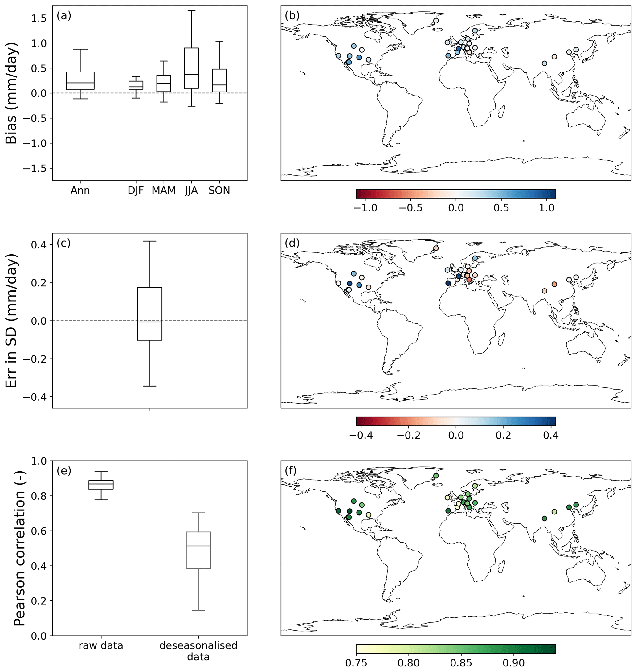
Figure 18 Comparison of Hydro-PE PETI calculated using interpolated and derived daily variables and Hydro-PE calculated using daily mean variables for 33 Northern Hemisphere grassland flux sites in the PLUMBER2 dataset. Panels (a), (c) and (e) show boxplots of the annual and seasonal bias (a), the error in the standard deviation (c), the Pearson correlation (e) of the raw data (black) and the deseasonalised data (grey). The bars show the whole range of the data. Panels (b), (d) and (f) show maps of the sites, coloured by the bias (b), the error in the standard deviation (d) and the Pearson correlation of the raw data (f).

We also compared the monthly median and the 10th and 90th percentiles of the PETI for each site calculated (a) using the daily mean meteorology, (b) using the meteorology derived and interpolated following the methods applied to HadUK-Grid, and (c) using the monthly mean meteorology (Fig. 19). The median is well represented, as are the summer 90th percentiles and the winter 10th percentiles. However, the PETI calculated using derived and interpolated input variables tends to overestimate the 90th percentile in the autumn and winter and overestimate the 10th percentile in the spring and summer compared to using the original daily means. However, despite this, it does perform better than simply using monthly mean inputs, which is equivalent to the use of MORECS monthly PE and which overestimates the 10th percentile and which underestimates the 90th percentile throughout the year. Most of the variability in the PETI calculated using derived and interpolated variables is due to using the daily air temperature and precipitation compared to using the monthly means of all the variables. There is a negligible difference between using the actual daily mean air temperature and the approximation using daily minimum and maximum temperatures (Eq. C1).

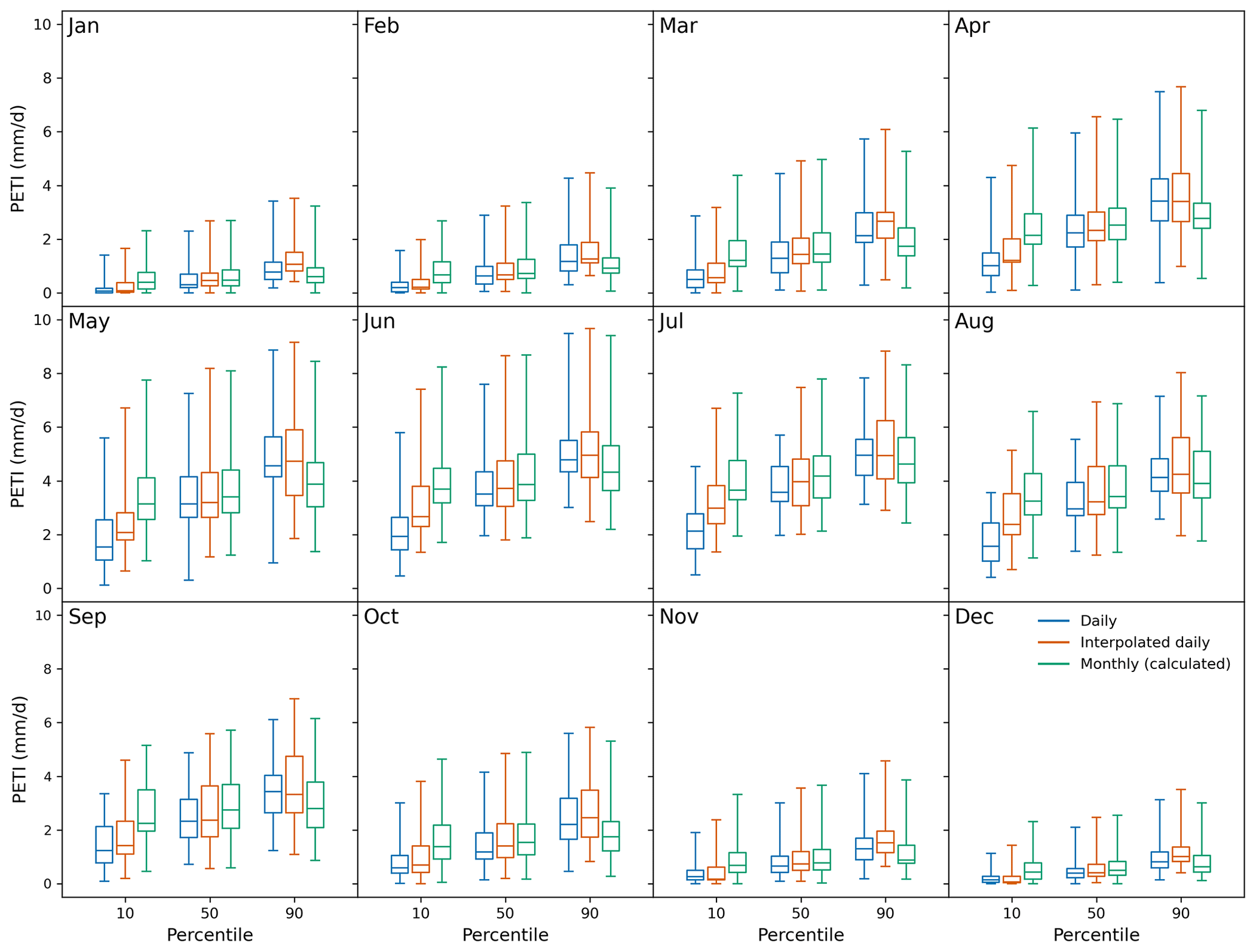
Figure 19 Monthly boxplots of the 10th, 50th and 90th percentiles of Hydro-PE PETI calculated using the daily PLUMBER2 data, the interpolated and derived PLUMBER2 variables as well as the derived PLUMBER2 variables at a monthly time step.

One source of the overall positive bias is the derived and interpolated net radiation, which has a high bias compared to the daily PLUMBER2 net radiation values, with mean bias error ranging between 3.39 and 51.9 W m⁻² across the sites. This is largely due to a high bias introduced in spring and summer by the calculation of short-wave radiation from sunshine hours (Sect. C6), which also causes the 10th percentiles of net radiation in the summer and the 90th percentiles of net radiation outside of the summer to be higher than those of the daily PLUMBER2 data. The temporal interpolation further enhances this impact on the extremes due to the effect of the reduced variability on the complex interplay between the different physical variables.

6 Discussion

These Hydro-PE datasets have been calculated with daily data. The Hydro-PE UKCP18 RCM data are self-consistent at a daily time step, having been calculated from climate model output. Care should be taken with Hydro-PE HadUK-Grid, however, as many of the input variables have been temporally downscaled from monthly to daily using a simple smooth interpolation. The variables have been interpolated independently of each other. The monthly means of Hydro-PE HadUK-Grid are consistent with the monthly meteorology and with monthly MORECS. The daily Hydro-PE HadUK-Grid is also consistent with daily MORECS PE (Sect. 5.2) and with daily EC site PETI (Sect. 5.3). However, there are some minor inconsistencies introduced by the temporal downscaling and conversion from the provided HadUK-Grid variables to the required inputs. In particular, this has caused an overestimation of winter and spring 90th percentiles. For applications sensitive to the winter and spring high extremes, users may consider winsorising the data when using them at a daily time step.

Past studies have seen that good results can be obtained by calculating PET at a monthly timescale (Allen et al., 1998; Oudin et al., 2010), and hydrological modelling in the UK is often carried out using monthly PE. For example, monthly MORECS is used to drive Grid-to-Grid (Bell et al., 2009) or CLASSIC (Crooks and Naden, 2007). For models which require daily PE inputs, using the temporally interpolated variables is an improvement on using monthly PE data, particularly as Hydro-PE HadUK-Grid uses daily (not interpolated) mean air temperature and precipitation.

Hydro-PE UKCP18 RCM has been calculated from an ensemble of climate model output that provides a range of possible future scenarios. The UKCP18 RCM ensemble only considers a single high-emissions scenario, RCP8.5 (Riahi et al., 2011), but the realisation of that scenario is different for each ensemble member due to differences in the input CO₂ concentration pathways and differences in the parameterisation of the climate model. This encapsulates not only the uncertainty in the global climate response to increased CO₂ concentrations, but also the uncertainty in the conversion of increased emissions to increased CO₂ concentrations (Murphy et al., 2018). RCP8.5 is the highest of the four RCPs that were developed by the climate modelling community after the Fourth Assessment Report (AR4; IPCC, 2007) to provide input to climate models and explore a range of emissions scenarios. The range of CO₂ concentration pathways used in the UKCP18 RCM ensemble was designed to approximate the spread of outcomes in the UKCP18 probabilistic projections, which included all four RCPs (Murphy et al., 2018). Hydro-PE UKCP18 RCM shows a large increase in both PET and PETI from the start to the end of the dataset alongside a change in the seasonality of the interception correction. Overall, these changes would be likely to be smaller under less extreme future emissions scenarios. Although the overall Hydro-PE UKCP18 RCM ensemble has large future changes, the lower end of the range of these changes may be consistent with more moderate future scenarios.

For users of climate model outputs, e.g. CMIP6 or UKCP18, calculating PET or PETI at a daily time step can involve large volumes of data or require variables that are unavailable at the daily time step. For PET, it is reasonable in this case to perform the calculations with monthly data (Oudin et al., 2010). However, PETI, which is corrected for interception based on precipitation, cannot reliably be calculated at a monthly time step. This is because, at a daily time step, the interception correction is only applied to rain days; dry days remain equal to PET. If a monthly mean precipitation is used to calculate the interception correction to monthly PET, then this is the equivalent of applying the interception correction to all days in the month, thus overestimating the PETI. One may calculate PET and PEI at the monthly time step, but it is essential to apply the interception correction based on the number of wet and dry days in the month. This can be done either by using daily precipitation to combine monthly PET and PEI appropriately or by using the number of wet and dry days in a month in combination with monthly precipitation and monthly PET and PEI, depending on the data available.

These datasets have only been calculated for one surface: short grass. This was chosen as it is a standard that is widely used. However, hydrology may be better represented by PE calculated for realistic land use. This could be done by parameterising the PE calculations appropriately for several different vegetation and other land use types and then combining appropriately for the given surface. The Hydro-PE calculations can easily be re-parameterised using vegetation characteristics. Equally, although these Hydro-PE datasets have been specifically parameterised and created for the UK, the method is flexible and can be parameterised and applied to meteorological data globally.

Apart from the effect of CO₂ on stomatal resistance, all of the other parameters have been kept constant throughout the period of future calculations, in particular the LAI, following Rudd and Kay (2016). While increased CO₂ can be expected to lead to increased biomass production, it is likely that the resultant effect on the LAI and the effect of the LAI on evaporation are actually small (Bunce, 2004), due either to the associated increase in shading or to nutrient limitation (Ainsworth and Long, 2005). Additionally, the short-grass cover that is being modelled here is similar to managed grasslands, which are likely to be artificially limited in LAI and height by human intervention. However, for other vegetation types, the effect of rising CO₂ may well have an impact on both the magnitude and the seasonality of physiological parameters, including LAI and canopy height. Future work should include this effect.

7 Code and data availability

The data can be downloaded from the Environmental Information Data Centre in netCDF format. Hydro-PE HadUK-Grid is available at https://doi.org/10.5285/9275ab7e-6e93-42bc-8e72-59c98d409deb (Brown et al., 2022), and Hydro-PE UKCP18 RCM is available at https://doi.org/10.5285/eb5d9dc4-13bb-44c7-9bf8-c5980fcf52a4 (Robinson et al., 2021).

The Python code used to perform the Hydro-PE calculations is available at https://doi.org/10.5281/zenodo.8363127 (Robinson, 2023).

8 Conclusions

We have demonstrated two new potential evaporation datasets for consistent historical and future hydrological modelling. They have been calculated using a method consistent with the widely used MORECS PE dataset and are parameterised for compatibility with models that have been calibrated to MORECS PE. Hydro-PE HadUK-Grid allows historical studies and calibration of hydrological models, while Hydro-PE UKCP18 RCM enables hydrological modelling to be carried out consistently into the future, accounting for climate change. This methodology is available for application to further climate model datasets, such as the convection-permitting model strand of UKCP18 (Kendon et al., 2021) and EuroCORDEX-UK (Barnes, 2023), which will enable consistent hydrological modelling across a range of climate projections.

Appendix A: Penman–Monteith equation

Potential evapotranspiration, E_p (mm d⁻¹), is calculated using the Penman–Monteith equation (Monteith, 1965) derived in terms of specific humidity (Stewart, 1989):

$$\begin{array}{}\text{(A1)}& E_{\mathrm{P}}={\displaystyle \frac{t_{\mathrm{D}}}{\mathit{\lambda }}}{\displaystyle \frac{{\mathrm{\Delta }}_q\left(R_{\mathrm{n}}-G\right)+\frac{{\mathit{\rho }}_{\mathrm{a}}{c}_{\mathrm{p}}}{r_{\mathrm{a}}}\left(q_{\mathrm{s}}-q_{\mathrm{a}}\right)}{{\mathrm{\Delta }}_q+{\mathit{\gamma }}_q\left(\mathrm{1}+\frac{r_{\mathrm{s}}}{r_{\mathrm{a}}}\right)}},\end{array}$$

where t_D=86 400 s d⁻¹ is the length of a day, $\mathit{\lambda }=\mathrm{2.5}\times {\mathrm{10}}^{-\mathrm{6}}$ J kg⁻¹ is the latent heat of vaporisation of water, q_s (kg kg⁻¹) is specific humidity at saturation, Δ_q (kg kg⁻¹ K⁻¹) is the gradient of specific humidity at saturation with respect to temperature, R_n (W m⁻²) is net radiation, G (W m⁻²) is ground heat flux, c_p=1010 J kg⁻¹ K⁻¹ is the specific heat capacity of air, ρ_a (kg m⁻³) is the density of air, q_a (kg kg⁻¹) is the specific humidity of air, ${\mathit{\gamma }}_q=c_{\mathrm{p}}/\mathit{\lambda }=\mathrm{0.004}$ K⁻¹ is the psychrometric constant for specific humidity, r_s (s m⁻¹) is canopy resistance, and r_a (s m⁻¹) is aerodynamic resistance.

Calculations for specific humidity at saturation and its gradient are given in Sects. A2 and A3. The ground heat flux, canopy resistance and aerodynamic resistance are calculated following MORECS: see Sect. E2–E4.

A1 Modified Penman–Monteith calculation

Since the meteorological variables provided in HadUK-Grid do not include net radiation values or surface temperature, we calculate the net radiation assuming that surface temperature T_* can be approximated by air temperature T_a. We then correct for this by calculating PE with a modified form of the Penman–Monteith equation as used in MORECS v2.0 (Hough et al., 1997):

$$\begin{array}{}\text{(A2)}& E_{\mathrm{P}}={\displaystyle \frac{t_{\mathrm{D}}}{\mathit{\lambda }}}{\displaystyle \frac{{\mathrm{\Delta }}_q\left(R_{\mathrm{ne}}-G\right)+\frac{{\mathit{\rho }}_{\mathrm{a}}{c}_{\mathrm{p}}}{r_{\mathrm{a}}}\left(q_{\mathrm{s}}-q_{\mathrm{a}}\right)\left(\mathrm{1}+\frac{b_R{r}_{\mathrm{a}}}{{\mathit{\rho }}_{\mathrm{a}}{c}_{\mathrm{p}}}\right)}{{\mathrm{\Delta }}_q+{\mathit{\gamma }}_q\left(\mathrm{1}+\frac{r_{\mathrm{s}}}{r_{\mathrm{a}}}\right)\left(\mathrm{1}+\frac{b_R{r}_{\mathrm{a}}}{{\mathit{\rho }}_{\mathrm{a}}{c}_{\mathrm{p}}}\right)}},\end{array}$$

where R_ne is the net radiation calculated using T_a as a proxy for surface temperature (see Sect. C8) and

$$\begin{array}{}\text{(A3)}& b_R=\mathrm{4}\mathit{ϵ}{\mathit{\sigma }}_{\mathrm{B}}{T}_{\mathrm{a}}\end{array}$$

is a correction for the radiative transfer between the surface and the screen height, with ϵ=0.95 the assumed surface emissivity as in MORECS (Hough et al., 1997) and ${\mathit{\sigma }}_{\mathrm{B}}=\mathrm{5.67}\times {\mathrm{10}}^{-\mathrm{8}}$ W m⁻² K⁻⁴ the Stefan–Boltzmann constant.

A2 Specific humidity at saturation

Saturated specific humidity, q_s, is derived as a function of temperature from the empirical fit of saturated vapour pressure, e_s, as a function of temperature (Richards, 1971):

$$\begin{array}{}\text{(A4)}& e_{\mathrm{s}}=p_{\mathrm{sp}}\exp \left(\sum _{i=\mathrm{1}}^{\mathrm{4}}{a}_i{\left(\mathrm{1}-{\displaystyle \frac{T_{\mathrm{sp}}}{T_{\mathrm{a}}}}\right)}^i\right),\end{array}$$

where p_sp=101 325 Pa is the steam point pressure, T_sp=373.15 K is the steam point temperature, and $a=(\mathrm{13.3185},-\mathrm{0.9760},-\mathrm{0.6445},-\mathrm{0.1299})$ are empirical coefficients.

In general, specific humidity, q_a, can be calculated from vapour pressure, e_a (hPa), using the function

$$\begin{array}{}\text{(A5)}& q_{\mathrm{a}}={\displaystyle \frac{{\mathit{ϵ}}_{\mathrm{a}}{e}_{\mathrm{a}}}{p_{*}-\left(\mathrm{1}-{\mathit{ϵ}}_{\mathrm{a}}\right)e_{\mathrm{a}}}},\end{array}$$

where p_* is the surface air pressure and ϵ_a=0.622 is the mass ratio of water to dry air (Gill, 1982).

Substituting the saturated vapour pressure from Eq. (A4) into the conversion between vapour pressure and specific humidity in Eq. (A5) gives an empirical function for saturated specific humidity of

$$\begin{array}{}\text{(A6)}& q_{\mathrm{s}}={\displaystyle \frac{{\mathit{ϵ}}_{\mathrm{a}}{p}_{\mathrm{sp}}\exp \left({\sum }_{i=\mathrm{1}}^{\mathrm{4}}{a}_i{\left(\mathrm{1}-\frac{T_{\mathrm{sp}}}{T_{\mathrm{a}}}\right)}^i\right)}{p_{*}-\left(\mathrm{1}-{\mathit{ϵ}}_{\mathrm{a}}\right)p_{\mathrm{sp}}\exp \left({\sum }_{i=\mathrm{1}}^{\mathrm{4}}{a}_i{\left(\mathrm{1}-\frac{T_{\mathrm{sp}}}{T_{\mathrm{a}}}\right)}^i\right)}}.\end{array}$$

A3 Derivative of specific humidity at saturation

The derivative of q_s with respect to air temperature, Δ_q (kg kg⁻¹ K⁻¹), can be calculated analytically from Eq. (A6) and is given by

$$\begin{array}{}\text{(A7)}& {\mathrm{\Delta }}_q={\displaystyle \frac{T_{\mathrm{sp}}}{T_{\mathrm{a}}^{\mathrm{2}}}}{\displaystyle \frac{q_{\mathrm{s}}}{{\mathit{ϵ}}_{\mathrm{a}}}}\left({\mathit{ϵ}}_{\mathrm{a}}+\left(\mathrm{1}-{\mathit{ϵ}}_{\mathrm{a}}\right)q_{\mathrm{s}}\right)\sum _{i=\mathrm{1}}^{\mathrm{4}}{a}_{i}i{\left(\mathrm{1}-{\displaystyle \frac{T_{\mathrm{sp}}}{T_{\mathrm{a}}}}\right)}^{i-\mathrm{1}}\end{array}$$

or

$$\begin{array}{}\text{(A8)}& {\mathrm{\Delta }}_q={\displaystyle \frac{T_{\mathrm{sp}}}{T_{\mathrm{a}}}}{\displaystyle \frac{p_{*}{q}_{\mathrm{s}}}{p_{*}-e_{\mathrm{s}}\left(\mathrm{1}-{\mathit{ϵ}}_{\mathrm{a}}\right)}}\sum _{i=\mathrm{1}}^{\mathrm{4}}i{a}_i{\left(\mathrm{1}-{\displaystyle \frac{T_{\mathrm{sp}}}{T_{\mathrm{a}}}}\right)}^{i-\mathrm{1}}.\end{array}$$

Appendix B: Interception correction

The PETI, E_PI (mm d⁻¹), is first calculated in the same way as PET. Then, on days with non-zero precipitation, an interception correction is applied. This is required because water that is intercepted by the canopy will evaporate at a faster rate than water that is transpired. Again, this is implemented following the MORECS v2.0 calculations (Hough et al., 1997). These calculations treat all precipitation as rainfall and do not allow for lying snow.

The amount of rainfall intercepted by the canopy, C_I (mm d⁻¹), is

$$\begin{array}{}\text{(B1)}& C_{\mathrm{I}}=\left\{\begin{array}{ll}P{f}_{\mathrm{P}}{e}_{\mathrm{P}}& \text{if}P{f}_{\mathrm{P}}<C_{\max },\\ C_{\max }{e}_{\mathrm{P}}& \text{otherwise},\end{array}\right.\end{array}$$

where $f_{\mathrm{P}}=\mathrm{1}-{\mathrm{0.5}}^{\mathrm{\Lambda }}$ is the LAI-dependent fraction of rainfall that would be intercepted if there were only one rain event on the day, C_max=0.2Λ (mm) is the maximum capacity of the canopy to hold water, and e_P is an enhancement factor to allow for the different character of rainfall throughout the year. In the winter, e_P is 1, but it rises to 2 in the summer, when the rain is likely to fall in multiple shorter, more intense, events. The monthly values of e_P are given in Table 2.

On a rain day, the intercepted fraction of rainfall is assumed to evaporate as an open water surface. This potential interception, E_I (mm d⁻¹), is calculated using Eq. (A1) with r_s=0 (all other parameters have the same value as for PET). The time taken to dry the canopy at this rate, t_dry (d), is calculated as

$$\begin{array}{}\text{(B2)}& t_{\mathrm{dry}}={\displaystyle \frac{C_{\mathrm{I}}}{E_{\mathrm{I}}}}.\end{array}$$

If this potential interception is enough to dry out the canopy in less than a day, then, for the rest of the day, it reverts to the rate of PET (E_P) such that

$$\begin{array}{}\text{(B3)}& E_{\mathrm{PI}}=t_{\mathrm{dry}}{E}_{\mathrm{I}}+\left(\mathrm{1}-t_{\mathrm{dry}}\right)E_{\mathrm{P}}.\end{array}$$

If it is not enough to dry out the canopy, then the PETI is equal to the potential interception E_I all day. The water remaining on the canopy is not carried over to the following day. By combining all these cases and combining Eqs. (B2) and (B3), the PETI is given by

$$\begin{array}{}\text{(B4)}& E_{\mathrm{PI}}=\left\{\begin{array}{ll}{E}_{\mathrm{P}}& \text{if}P=\mathrm{0},\\ E_{\mathrm{P}}+C_{\mathrm{I}}\left(\mathrm{1}-\frac{E_{\mathrm{P}}}{E_{\mathrm{I}}}\right)& \text{if}P>\mathrm{0}\text{and}{C}_{\mathrm{I}}<E_{\mathrm{I}},\\ E_{\mathrm{I}}& \text{if}P>\mathrm{0}\text{and}{C}_{\mathrm{I}}\ge E_{\mathrm{I}}.\end{array}\right.\end{array}$$

Appendix C: Calculation of input variables for Hydro-PE HadUK-Grid

C1 Temporal interpolation of meteorology

The sunshine hours, wind speed, vapour pressure and sea level air pressure were interpolated from monthly to daily time steps using quadratic interpolation from Python's scipy package (Virtanen et al., 2020), assuming that the monthly values represent the 15th day of each month. The sunshine hours were divided by the number of days in each month to get an average daily value before interpolation. We constrained sunshine hours and vapour pressure to always be positive in order to avoid some unphysical negative values that were a result of extrapolation of the quadratic interpolation at either end of the time series. Following the temporal interpolation, the required input variables were calculated from the interpolated and existing daily variables as follows.

C2 Daily mean air temperature

We approximate the daily mean air temperature from the daily minimum and maximum air temperatures using

$$\begin{array}{}\text{(C1)}& T_{\mathrm{a}}={\displaystyle \frac{T_{\min }+T_{\max }}{\mathrm{2}}}.\end{array}$$

C3 Surface air pressure

Both the specific humidity at saturation and its derivative are functions of both air temperature and surface air pressure at the grid box elevation. As HadUK-Grid only provides sea level air pressure, p_SL (hPa), we must calculate the air pressure at the grid box elevation. The sea level air pressure is adjusted to the grid box elevation by assuming a constant local environmental lapse rate for air temperature of ${\mathrm{\Gamma }}_T=-\mathrm{0.006}$ K m⁻¹ (as used in Hough et al., 1997; Robinson et al., 2017). The surface air pressure at a given elevation, p_* (hPa), is calculated using the integral of the hypsometric equation (Shuttleworth, 2012) so that

$$\begin{array}{}\text{(C2)}& p_{*}=p_{\mathrm{SL}}{\left({\displaystyle \frac{T_{\mathrm{a}}-z{\mathrm{\Gamma }}_T}{T_{\mathrm{a}}}}\right)}^{\frac{g}{r{\mathrm{\Gamma }}_T}},\end{array}$$

where T_a (K) is the air temperature at the grid box elevation, z (m) is the grid box elevation above sea level, g=9.81 m s⁻² is acceleration due to gravity, and r=287.05 J kg⁻¹ K⁻¹ is the specific gas constant of dry air.

C4 Air density

The density of air, ρ_a, was calculated from the surface air pressure and the air temperature, such that

$$\begin{array}{}\text{(C3)}& {\mathit{\rho }}_{\mathrm{a}}={\displaystyle \frac{p_{*}}{r{T}_a}},\end{array}$$

where r=287.05 J kg⁻¹ K⁻¹ is the gas constant of dry air.

C5 Specific humidity

The specific humidity is calculated using the water vapour pressure (e_a) and surface pressure (p_*) using Eq. (A5).

C6 Net short-wave surface radiation

Downward short-wave radiation, S_d (W m⁻²), is calculated from sunshine hours following the MORECS procedure and using Eq. (4.14)–(4.19) of Hough et al. (1997). Equation (4.14) yields the total radiation integrated over the day (W h m⁻²), so to get the daily average, this was divided by 24, the number of hours in a day, such that

$$\begin{array}{}\text{(C4)}& S_{\mathrm{d}}={\displaystyle \frac{\mathrm{1}}{\mathrm{24}}}{R}_{\mathrm{a}}\left(\mathit{\eta }\left(a_{\mathrm{A}}+b_{\mathrm{A}}{\displaystyle \frac{t_{\mathrm{S}}}{t_N}}\right)+c_{\mathrm{A}}\left(\mathrm{1}-\mathit{\eta }\right)\right),\end{array}$$

where a_A, b_A and c_A are the Ångström coefficients, R_a is the top-of-atmosphere radiation integrated over a day (W h m⁻²), t_S is the measured hours of bright sunshine in the day, t_N is the length of daylight hours (sunrise to sunset) (Hough et al., 1997), and η is

$$\begin{array}{}\text{(C5)}& \mathit{\eta }=\left\{\begin{array}{ll}\mathrm{0}& \text{if}{t}_{\mathrm{S}}=\mathrm{0},\\ \mathrm{1}& \text{if}{t}_{\mathrm{S}}>\mathrm{0}.\end{array}\right.\end{array}$$

The Ångström coefficients are empirical constants that are used to calculate solar radiation from sunshine hours. They were calculated on the MORECS 40 km grid by Cowley (1978). For this study they were then interpolated onto the 1 km HadUK grid using a smooth bivariate spline. They were only available for England, Scotland and Wales, and so the coefficients for Northern Ireland were spatially extrapolated. They are close to the “default” values suggested for use by the FAO when local calibration is not available (see Eq. 35 in Allen et al., 1998). a_A and c_A are constant in time, whereas b_A varies by month. Here, the b_A coefficient is interpolated onto a daily time step using a periodic cubic spline (periodic so that there is no discontinuity between the values for 31 December and 1 January).

R_a and t_N are calculated as

$$\begin{array}{}\text{(C6)}& \begin{array}{rl}{R}_{\mathrm{a}}& =t_{\mathrm{S}}\left(\left(t_{\mathrm{2}}-t_{\mathrm{1}}\right)\sin \mathit{\delta }\sin \mathit{\varphi }\right.\\ & \left.+{\displaystyle \frac{\mathrm{12}\cos \mathit{\delta }\cos \mathit{\varphi }\left(\sin \frac{\mathit{\pi }{t}_{\mathrm{1}}}{\mathrm{12}}-\sin \frac{\mathit{\pi }{t}_{\mathrm{2}}}{\mathrm{12}}\right)}{\mathit{\pi }}}\right)\end{array}\end{array}$$

and

$$\begin{array}{}\text{(C7)}& t_N=t_{\mathrm{2}}-t_{\mathrm{1}},\end{array}$$

where t₁ and t₂ are sunrise and sunset times, ϕ is the latitude, and δ is the solar declination angle calculated from the day of the year d using

$$\begin{array}{}\text{(C8)}& \mathit{\delta }=\mathrm{0.41}\cos \mathrm{2}\mathit{\pi }{\displaystyle \frac{d-\mathrm{172}}{\mathrm{365}}}.\end{array}$$

Sunrise, t₁ (h), is calculated using

$$\begin{array}{}\text{(C9)}& t_{\mathrm{1}}={\displaystyle \frac{\mathrm{12}}{\mathit{\pi }}}\arccos \left(\tan \mathit{\delta }\tan \mathit{\varphi }+{\displaystyle \frac{\mathrm{0.0145}}{\cos \mathit{\delta }\cos \mathit{\varphi }}}\right),\end{array}$$

and sunset, t₂ (h), is given by

$$\begin{array}{}\text{(C10)}& t_{\mathrm{2}}=\mathrm{24}-t_{\mathrm{1}}.\end{array}$$

Net short-wave radiation is calculated from downward short-wave radiation using albedo, α, as

$$\begin{array}{}\text{(C11)}& S_{\mathrm{n}}=\left(\mathrm{1}-\mathit{\alpha }\right)S_{\mathrm{d}}.\end{array}$$

The albedo values used are described in Sect. E1.

C7 Estimate of net long-wave surface radiation

The calculation of L_ne followed MORECS, documented in more detail in Hough et al. (1997), using air temperature, vapour pressure and sunshine hours via

$$\begin{array}{}\text{(C12)}& L_{\mathrm{ne}}=\mathit{ϵ}{\mathit{\sigma }}_{\mathrm{B}}{T}_{\mathrm{a}}^{\mathrm{4}}\left(\mathrm{1.28}{\left({\displaystyle \frac{e}{T_{\mathrm{a}}}}\right)}^{\frac{\mathrm{1}}{\mathrm{7}}}-\mathrm{1}\right)\left(\mathrm{0.2}+\mathrm{0.8}{\displaystyle \frac{t_{\mathrm{S}}}{t_N}}\right).\end{array}$$

Note that this is only an approximation of net long-wave radiation, as it has made use of an approximation when calculating the upward component of the radiation, L_u. Normally, upward long-wave radiation is calculated from surface temperature:

$$\begin{array}{}\text{(C13)}& L_{\mathrm{u}}=\mathit{ϵ}{\mathit{\sigma }}_{\mathrm{B}}{T}_{*}^{\mathrm{4}}.\end{array}$$

However, if surface temperature is not available, then an approximate upward long-wave radiation, L_ue, can be calculated by substituting $T_{\mathrm{a}}\approx T_{*}$ into Eq. (C13). This approximation has been carried through to the approximate net long-wave radiation in Eq. (C12).

The approximate net long-wave radiation is related to the actual net long-wave radiation, L_n, by the relationship

$$\begin{array}{}\text{(C14)}& L_{\mathrm{ne}}=L_{\mathrm{n}}-b_R\left(T_{\mathrm{a}}-T_{*}\right),\end{array}$$

where b_R is given by Eq. (A3).

C8 Approximate net radiation

After deriving the approximate net long-wave radiation and net solar radiation, the approximate net radiation, R_ne (W m⁻²), is simply calculated by summing these two components:

$$\begin{array}{}\text{(C15)}& R_{\mathrm{ne}}=L_{\mathrm{ne}}+S_n.\end{array}$$

That this is an approximation means that we must use a modified form of the Penman–Monteith equation described in Sect. A1.

Appendix D: Calculation of input variables for Hydro-PE UKCP18 RCM

D1 Net radiation

The UKCP18 dataset contains net long-wave radiation, L_n (W m⁻²), and net short-wave radiation, S_n (W m⁻²). Therefore the total net radiation is given by

$$\begin{array}{}\text{(D1)}& R_{\mathrm{n}}=L_{\mathrm{n}}+S_{\mathrm{n}}.\end{array}$$

D2 Surface air pressure

The daily pressure at mean sea level is adjusted to the pressure at the grid box surface height following Eq. (C2).

D3 Air density

The air density was calculated from surface air pressure and air temperature using Eq. (C3).

Appendix E: Surface parameters

E1 Albedo

The albedo α is also calculated following MORECS as a combination of the albedo of the grass, α_g, and the albedo of the underlying soil, α_s:

$$\begin{array}{}\text{(E1)}& \mathit{\alpha }=\left\{\begin{array}{ll}{\mathit{\alpha }}_{\mathrm{g}}& \text{if}\mathrm{\Lambda }>\mathrm{4},\\ {\mathit{\alpha }}_{\mathrm{s}}+\mathrm{0.25}\mathrm{\Lambda }\left({\mathit{\alpha }}_{\mathrm{g}}-{\mathit{\alpha }}_{\mathrm{s}}\right)& \text{otherwise},\end{array}\right.\end{array}$$

where Λ is the LAI (Hough et al., 1997).

The albedo of grass is taken to be the MORECS value for soils with median available water content (AWC) α_g=0.25. Soil albedo is dependent on whether the soil is wet or dry: for wet soils, α_s=0.1, and for dry soils, α_s=0.2. A soil is considered wet if there has been precipitation in the day and is considered dry otherwise. MORECS also provides values for soils with high AWC and low AWC, but these were not used for this calculation, as soil properties are not considered.

E2 Ground heat flux

For the ground heat flux, the average monthly value of ground heat storage as used in MORECS v2.0 was used (see Table 2). This is a monthly mean of daily heat storage estimated from measurements of soil temperature (Wales-Smith and Arnott, 1980). The monthly value was converted into a daily flux and applied to all days in that month.

E3 Aerodynamic resistance

Aerodynamic resistance r_a (s m⁻¹) is calculated as a function of the roughness length of the canopy z₀ (h) using the MORECS equation:

$$\begin{array}{}\text{(E2)}& r_{\mathrm{a}}={\displaystyle \frac{\mathrm{6.25}}{u_{\mathrm{10}}}}\ln {\displaystyle \frac{\mathrm{10}}{z_{\mathrm{0}}}}\ln {\displaystyle \frac{\mathrm{6}}{z_{\mathrm{0}}}},\end{array}$$

where u₁₀ is the wind speed at 10 m above the canopy, and

$$\begin{array}{}\text{(E3)}& z_{\mathrm{0}}={\displaystyle \frac{h}{\mathrm{10}}},\end{array}$$

where h is the canopy height of grass. Following MORECS v2.0, grass is assumed to be 0.15 m high.

E4 Canopy resistance

The canopy resistance is a combination of the stomatal resistance of the canopy, r_sc (s m⁻¹), and the surface resistance of a bare soil surface, r_ss (s m⁻¹), following MORECS v2.0 (Hough et al., 1997), such that

$$\begin{array}{}\text{(E4)}& {\displaystyle \frac{\mathrm{1}}{r_{\mathrm{s}}}}={\displaystyle \frac{\mathrm{1}-{\mathrm{0.7}}^{\mathrm{\Lambda }}}{r_{\mathrm{sc}}}}+{\displaystyle \frac{{\mathrm{0.7}}^{\mathrm{\Lambda }}}{r_{\mathrm{ss}}}},\end{array}$$

where Λ is the LAI of the grass surface. The LAI was assumed to vary throughout the year, and monthly values are taken from MORECS v2.0 (see Table 2). This seasonal cycle of LAI was kept the same through the full time coverage of the calculations.

E5 CO₂ fertilisation effect

The stomatal resistance was also assumed to vary monthly through the year. In addition, it was assumed that stomatal resistance will increase in the future due to projected rising CO₂ levels (Rudd and Kay, 2016). The baseline historical stomatal resistance of grass, r_scM (s m⁻¹), was taken from MORECS v2.0 (Hough et al., 1997) (see Table 2). For years up to the baseline year of 1981, the stomatal resistance was assumed to stay constant. From 1981 onwards the stomatal resistance was then adjusted for changes in CO₂ concentration following the method of Kruijt et al. (2008), so that for each month, m, and year, y, the stomatal resistance is

$$\begin{array}{}\text{(E5)}& r_{\mathrm{sc}}[y,m]=\left\{\begin{array}{ll}{r}_{\mathrm{scM}}\left[m\right]& \text{if}y\le \mathrm{1981},\\ \frac{r_{\mathrm{scM}}\left[m\right]}{\mathrm{1}-\mathrm{0.00093}\left({\mathrm{CO}}_{\mathrm{2}}\left[y\right]-{\mathrm{CO}}_{\mathrm{2}}\left[\mathrm{1981}\right]\right)}& \text{if}y>\mathrm{1981},\end{array}\right.\end{array}$$

where CO₂[y] is the CO₂ concentration (ppmv) in the year y and 1981 is the reference year. As each ensemble member of the UKCP18 RCM ensemble was run with a different CO₂ concentration (Murphy et al., 2018), this adjustment of the stomatal resistance was calculated separately for each ensemble member using the corresponding CO₂ trajectory (Met Office Hadley Centre, 2020a).

The surface resistance of bare soil was set to 100 m s⁻¹, again following MORECS v2.0 (Hough et al., 1997).