the Creative Commons Attribution 4.0 License.
the Creative Commons Attribution 4.0 License.
 | 04 Sep 2023
A new 2010 permafrost distribution map over the Qinghai–Tibet Plateau based on subregion survey maps: a benchmark for regional permafrost modeling
Zetao Cao
Jianan Hu
Yuhong Chen
Yaonan Zhang
Permafrost over the Qinghai–Tibet Plateau (QTP) has received increasing attention due to its high sensitivity to climate change. Numerous spatial modeling studies have been conducted on the QTP to assess the status of permafrost, project future changes in permafrost, and diagnose contributors to permafrost degradation. Due to the scarcity of ground stations on the QTP, these modeling studies are often hampered by the lack of validation references, calibration targets, and model constraints; however, a high-quality permafrost distribution map would be a good option as a benchmark for spatial simulations. Existing permafrost distribution maps for the QTP can poorly serve this purpose. An ideal benchmark map for spatial modeling should be methodologically sound, of sufficient accuracy, and based on observations from mapping years rather than all historical data spanning several decades. Therefore, in this study, we created a new permafrost distribution map for the QTP in 2010 using a novel permafrost mapping approach with satellite-derived ground surface thawing and freezing indices as inputs and survey-based subregion permafrost maps as constraints. This approach accounted for the effects of local factors by incorporating (into the model) an empirical soil parameter whose values were optimally estimated through spatial clustering and parameter optimization constrained by survey-based subregion permafrost maps, and the approach was also improved to reduce parametric equifinality. This new map showed a total permafrost area of about 1.086×10⁶ km2 (41.2 % of the QTP area) and seasonally frozen ground of about 1.447×10⁶ km2 (54.9 %) in 2010, excluding glaciers and lakes. Validations using survey-based subregion permafrost maps (κ=0.74) and borehole records (overall accuracy =0.85 and κ=0.43) showed a higher accuracy of this map compared with two other recent maps. Inspection of regions with obvious distinctions between the maps affirms that the permafrost distribution on this map is more realistic than that on the Zou et al. (2017) map. Given the demonstrated excellent accuracy, this map can serve as a benchmark map for constraining/validating land surface simulations on the QTP and as a historical reference for projecting future permafrost changes on the QTP in the context of global warming. The dataset is available from the repository hosted on Figshare (Cao et al., 2022): https://doi.org/10.6084/m9.figshare.19642362.
- Article
(15623 KB) - Full-text XML
- BibTeX
- EndNote


Permafrost, defined as ground that remains at or below 0 ∘C for at least 2 consecutive years (Dobinski, 2011), underlies more than 20 % of the exposed land area in the Northern Hemisphere (Obu et al., 2019) and constitutes an essential component of the Earth system. The Qinghai–Tibet Plateau (QTP), also known as the Earth's third pole, contains the largest mid- to low-latitude permafrost area in the world. Due to the complex topography and unique plateau climate, permafrost over the QTP is generally of low thermal stability and strongly influenced by complex local factors, such as terrain, vegetation cover, soil properties, and hydrological conditions, which differentiate it from high-latitude permafrost around the Arctic and make it more sensitive to global climate change (Li et al., 2008; Yang et al., 2019; Zhao et al., 2020).
In the context of global warming, significant permafrost degradation is occurring on the QTP and has strongly affected hydrological processes (Li et al., 2020), carbon cycling (Mu et al., 2020), and heat exchange processes (Zhao et al., 2020). In addition, hazards related to permafrost degradation threaten construction and infrastructure on the QTP (Wang et al., 2020). Many researchers have studied the complex responses and feedback of permafrost to climate change (Yang et al., 2019), while land surface model-based spatial modeling of permafrost has become an important approach (Ji et al., 2022). Using land surface models, many spatial modeling studies have attempted to project future changes in permafrost (Chang et al., 2018; Debolskiy et al., 2020; Yin et al., 2021), assess the permafrost status under climate change (Koven et al., 2013; Burke et al., 2020), diagnose the contributors to regional permafrost degradation (Zhang et al., 2021a, b; Mekonnen et al., 2021), and project potential feedbacks on the climate system due to permafrost degradation (Zhang et al., 2020; Andresen et al., 2020; Yokohata et al., 2020; Wang et al., 2021). However, evaluating the spatial simulations for the QTP can be challenging due to the limited availability of ground observations, which may not be sufficient to serve as references across the vast spatial modeling domain. Hence, there is a need for an accurate permafrost distribution map that would serve as a reference to validate the results of spatial simulations. The map could be used as a target for the calibration of model parameters and to provide a constraint for future projections to minimize biases resulting from the modeling process. Moreover, an accurate map of permafrost distribution could serve as a fundamental dataset for hydrological, carbon, ecological, and engineering studies in cold regions (Hu et al., 2019a; Li et al., 2020; Song et al., 2020; Mu et al., 2020).
Although many permafrost distribution maps have been compiled over the QTP (Cheng et al., 2011; Shi and Mi, 2013; Wang, 2013; Guo and Wang, 2013; Zou et al., 2017; Niu and Yin, 2018; Shi et al., 2018; Wu et al., 2018; Wang et al., 2019c), few of them can serve as benchmarks for calibrating and validating land surface models (Wang et al., 2016; Cao et al., 2019a). The accuracy of existing maps is constrained by the limited availability and quality of data used to create them as well as by the inadequacy of mapping approaches. Early permafrost maps on the QTP (Cheng et al., 2011; Shi and Mi, 2013) were compiled through visual interpretation based on a limited number of data and expert judgment. Subsequently, satellite data and reanalysis data have become the main data sources of permafrost mapping (Wang, 2013; Zou et al., 2017; Shi et al., 2018; Wang et al., 2019c). However, large gaps in satellite data coverage caused by clouds would highly affect the accuracy of permafrost maps in the absence of effective interpolation methods (Chen et al., 2020). Although the reanalysis products do not suffer from cloud contamination, their coarse spatial resolutions and associated large uncertainties on the QTP (Hu et al., 2019b; Qin et al., 2020; Cao et al., 2020) would limit the accuracy of the derived maps.
Uncertainties associated with mapping approaches also negatively impact the accuracy of existing permafrost maps. Common statistical learning methods for permafrost mapping (Wang et al., 2019c; Ni et al., 2021) heavily rely on in situ observations as a training dataset. Therefore, they are often compromised when ground observations are unevenly distributed and have different observation periods, as is the case for the QTP. This led to misrepresentation and overfitting in permafrost maps (Marcer et al., 2017). Meanwhile, the lack of accurate soil properties, fine-tuned parameterization schemes, and high-resolution forcing data on the QTP severely challenged the applications of land surface models in mapping permafrost (Wu et al., 2018). These physically explicit models were often calibrated and validated at a point scale, leading to unpredictable uncertainties when extended to a large region with more variability and, thus, more complex conditions (Qin et al., 2017; Wu et al., 2018). In addition, permafrost distribution maps generated by land surface models are usually not well suited as independent benchmark maps, as the land surface models are more or less similar in terms of model structure and forcing data. Therefore, empirical and semi-physical approaches remain the mainstay of permafrost mapping on the QTP, as they require fewer in situ observations than statistical learning methods and have a simpler structure with fewer parameters than physical models (Zou et al., 2017; Zhao et al., 2017). Nevertheless, these maps have been criticized for limited consideration of local factors (Cao et al., 2019a; Hu et al., 2020) and the lack of constraints imposed to avoid divergence. All of these issues call into question the ability of the existing permafrost distribution maps to serve as benchmark maps for land surface simulations on the QTP.
An ideal benchmark map for spatial modeling of permafrost should fulfill the following criteria:
-
It should be based on an adequate number of robust observations that have not already been used for the simulation.
-
It should be based on the data from the mapping year, rather than all data spanning decades while they were still available; this is especially important if the benchmark map is used to calibrate a transient model.
-
It should account for the influences of local factors and be well constrained during the mapping process.
Based on these criteria, this study aims to produce a permafrost distribution map over the QTP in 2010 through an effective permafrost mapping approach that considers the effects of local factors and utilizes observational data, including remote sensing data and survey-based subregion permafrost maps, as optimization targets and constraints. Our objective is to provide a new reference map for 2010 for permafrost studies on the QTP and to provide a benchmark map for transient simulations of QTP permafrost under climate change.
2.1 Study area
The QTP (bounded within 26–40∘ N and 73.5–104.5∘ E) is a high-elevation flat terrain of about 2.6×10⁶ km2 and is surrounded by high mountain ranges (Fig. 1). The northwestern region of the QTP is predominantly characterized by alpine desert, gradually transitioning towards alpine meadow and forest in the southeastern part (Wang et al., 2016). Most of the QTP lies between 3000 and 5000 m a.s.l. (above sea level) with an average of about 4000 m a.s.l. The mean annual air temperature varied between −5 and 5 ∘C in most areas during the period from 1981 to 2010, with July experiencing the highest monthly temperature of about 10 ∘C and January recording the lowest at −10 ∘C. Between 1960 and 2010, air temperature increased by about 0.3–0.4 ∘C per decade, which is more than twice the global warming rate (Zhang et al., 2019). Mean annual precipitation decreases from more than 700 mm in the southeast to about 50 mm in the northwest, and about 90 % of precipitation falls during the growing season from May to September (Peng et al., 2019). Snow cover on the QTP is thin and of short duration (Wu and Zhang, 2008). Extensive alpine permafrost has formed across the QTP, featuring continuous permafrost in the central region and discontinuous permafrost in the southern parts (Yi et al., 2014). Ice-rich layers are commonly observed near the permafrost table on the plateau, which typically reaches a depth of 2–3 m (Zhao et al., 2020). Permafrost thickness on the QTP ranges from several meters to about 350 m, while the depth of zero annual amplitude varies from 3.5 to 17 m (Zhao et al., 2020). The QTP permafrost is also characterized by a high mean annual ground temperature (MAGT), which is above −3 ∘C in most permafrost regions (Zhao et al., 2020).
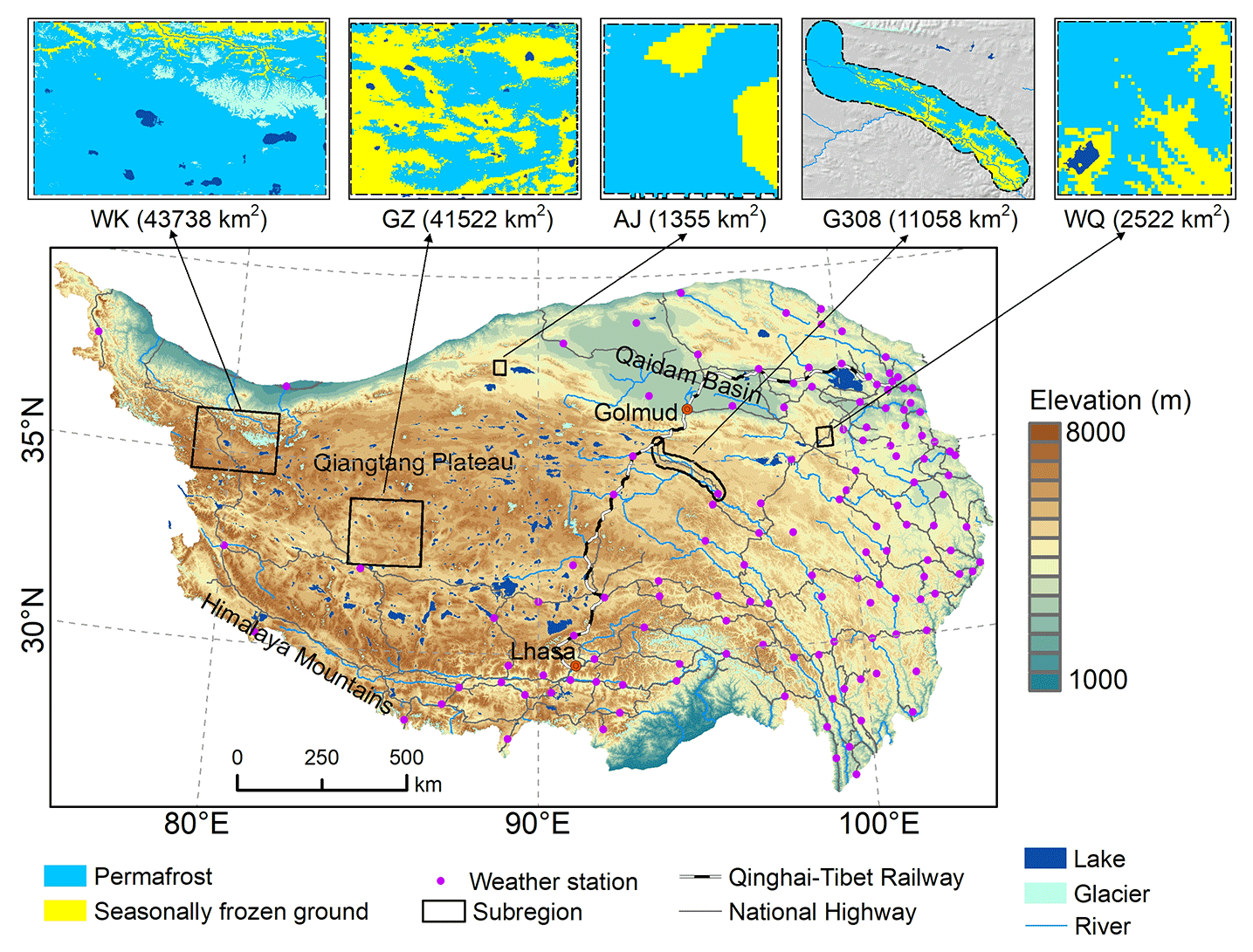
Figure 1Map showing the topography of the Qinghai–Tibet Plateau (QTP), the locations of meteorological stations, and the subregions with extensive field surveys. Inset maps show the local permafrost distributions in the five subregions based on the survey data of ca. 2010: WK, West Kunlun; GZ, Gaize; AJ, Aerjin; WQ, Wenquan; and G308, national highway G308.
2.2 Subregion permafrost maps
From 2009 to 2014, a research project sponsored by the Chinese Minister of Science and Technology was carried out to investigate permafrost and its surroundings. Intensive surveys were conducted in five areas (i.e., West Kunlun, Gaize, Aerjin, national highway G308, and Wenquan; see Fig. 1), each characterized by distinct climatic and geographic conditions and representative of the different permafrost environments on the QTP (Zhao et al., 2017). Comprehensive information was acquired through field observations, mechanical excavations, geophysical reconnaissance techniques (e.g., ground-penetrating radar, GPR, and time-domain electromagnetic surveys), and borehole drilling, which allowed for the mapping of the permafrost distribution with high accuracy in all five subregions. The permafrost distribution in the Wenquan and West Kunlun subregions was mapped by a multivariate adaptive regression splines (MARS) model trained on large samples from field surveys: 130 GPR profiles and 21 boreholes in Wenquan and 103 GPR profiles, 50 pits, and 13 boreholes in West Kunlun. In the Gaize, Aerjin, and G308 subregions, the maps were based on aspect-stratified relationships between the altitudinal limits of permafrost and topography (Chen et al., 2016).
These subregion permafrost maps have been widely used as ground truth in many modeling studies (Zou et al., 2017; Zhao et al., 2017; Shi et al., 2018; Wu et al., 2018; Wang et al., 2019b). The original maps have a spatial resolution of 250 m. In this study, these maps were aggregated, resampled to a 1 km resolution, and then used to calibrate an empirical soil parameter representing a synthesized soil thermal and moisture condition.
2.3 Satellite land surface temperature product
The land surface temperature (LST) data product from the Moderate Resolution Imaging Spectroradiometer (MODIS) aboard the Terra and Aqua satellites is one of the most widely used LST products due to its high spatial and temporal resolutions (Wan, 2008). It has a global coverage and has been applied in many permafrost mapping studies to provide temperature conditions (Gisnås et al., 2017; Zou et al., 2017; Obu et al., 2019; Wang et al., 2019c). In this study, the daily MODIS LST and emissivity products (MOD11A1 and MYD11A1 Version 6) were used, providing up to two daytime and two nighttime LST observations at a 1 km resolution. These observations were used to estimate annual ground surface thawing (DDT) and freezing indices (DDF) driving the mapping approach. DDT and DDF are defined as the absolute values of the cumulative degree-days throughout a year when ground surface temperatures (GSTs) are above and below 0 ∘C, respectively (Nelson and Outcalt, 1987). In practice, multiyear average DDTs (DDFs) are used instead of a single-year DDT (DDF) in order to mitigate the impact of single-year meteorological anomalies. In addition, the presence of permafrost is, by definition, determined by the thermal conditions of the last 2 years, indicating that not only the DDT and DDF of the current year but also those of previous years influence the presence of permafrost. We finally used the period from 2005 to 2010 to derive the DDT and DDF for 2010, partly because automatic weather stations have been commissioned on the QTP since 2005, which we needed to accomplish the DDT estimation from the MODIS LST data.
2.4 Environmental factors influencing permafrost distribution
In our approach, we spatially divided the study area into different soil clusters to represent the heterogeneity of permafrost environments on the QTP on the basis of several environmental factors. The composite 16 d 1 km normalized difference vegetation index (NDVI) product (MOD13A2) provides information on vegetation greenness and has been shown to be well suited to differentiate the main vegetation classes on the QTP (Zhao et al., 2015). We calculated the average aggregate from 2005 to 2010 and used it as an attribute for spatial clustering and as a predictor variable for estimating DDT. Topographical factors, including elevation and slope, were derived from the Shuttle Radar Topography Mission 90 m digital elevation database (SRTM DEM, version 4; Reuter et al., 2007) and then aggregated to a working spatial resolution of 1 km. The STRM-derived topographic wetness index (TWI), along with mean annual precipitation from 2005 to 2010 aggregated from the 1 km monthly precipitation dataset for China (Peng et al., 2019), represents wetness conditions affecting permafrost distribution. Likewise, average aggregate fraction snow cover (FSC) data were processed for the same period from the 500 m Daily Fractional Snow Cover Dataset Over High Asia (Qiu et al., 2017). Soil texture-type data derived from the China Data Set of Soil Properties for Land Surface Modeling (Shangguan et al., 2013) were also included.
2.5 In situ observations
2.5.1 Ground surface temperature (GST) observations
There are 131 national meteorological stations of China on the QTP (Fig. 1), which are mostly concentrated in the eastern QTP. At these stations, standard meteorological variables, including air pressure, air temperature, precipitation, evaporation, relative humidity, wind speed and direction, sunshine hours, and 0 cm ground surface temperature, are measured four times a day, at 02:00, 08:00, 14:00, and 20:00 (UTC+8). We extracted the daily GST observations during the period from 2005 to 2010 at these stations from the daily meteorological dataset of basic meteorological elements of the China National Surface Weather Station (V3.0) (National Meteorological Information Centre, 2019). The in situ GST observations were used to estimate DDTs from the satellite LSTs on the QTP.
2.5.2 Permafrost presence/absence observations
We used permafrost presence/absence information from boreholes to evaluate the new permafrost distribution map produced in this study. These data are independent of those used to produce subregion permafrost maps and come primarily from three sources.
First, a newly published synthesis dataset of permafrost thermal state on the QTP (Zhao et al., 2021) provides 65 boreholes where soil temperatures at 10 and 20 m depths were monitored for 2005–2018. Thus, the presence of permafrost at borehole locations around 2010 was determined based on mean annual soil temperatures at the two aforementioned depths, as previous evidence suggests that the depths of zero annual amplitude at these locations are within the two depths. These boreholes were further classified into three categories: boreholes with stable permafrost (mean annual soil temperature below −0.1 ∘C at either depth), boreholes with unstable permafrost (above −0.1 ∘C at both depths and below 0 ∘C at either depth), and boreholes with seasonal frost (above 0 ∘C at both depths).
Second, seven boreholes were collected from existing literature (Li et al., 2016) that provided information on permafrost presence in the Yellow River source area, a key region in the eastern QTP. Ground temperatures in these boreholes were measured in the summers of 2013 and 2014 and assumed to reflect the thermal regimes in 2010. The borehole locations were classified as seasonal frost if soil temperatures at a 15 m depth were above 0 ∘C, otherwise they were classified as permafrost.
Third, in the Yangtze River source area, an important, ecologically vulnerable permafrost region of the QTP, recent observations of the presence/absence of permafrost in 2020 from 32 boreholes (Li et al., 2022) were also used as a reference. Because permafrost on the QTP has warmed in recent decades (Cheng et al., 2019), some boreholes indicative of the presence of seasonally frozen ground (SFG) in 2020 may have appeared to be permafrost in 2010. Therefore, these 32 boreholes were not used to quantitatively validate the results but rather only as an aid for comparison.
2.6 Existing QTP permafrost maps for comparison
To better evaluate the new map produced in this study, two peer permafrost distribution maps with a resolution of 1 km were used. One was compiled by Zou et al. (2017) using the temperature at the top of permafrost model (TTOP) and MODIS LST data from 2003 to 2012 (hereinafter referred to as the Zou map). The other map was developed via a data-driven approach by Wang et al. (2019) (hereinafter referred to as the Wang map) with samples from two previous maps: (1) a 2006 map (Wang, 2013) with the QTP portion mapped using a multilinear regression model (Nan et al., 2002) and (2) the Zou map. MODIS LST data were also used as a predictor variable for the Wang map. Recently, the Zou map has been widely used to represent permafrost distribution around 2010 and has served as the ground truth in many QTP studies (Hu et al., 2019a; Song et al., 2020; Mu et al., 2020; Ni et al., 2021; Yin et al., 2021). Cao et al. (2019a) evaluated the Zou map as the best-performing permafrost map on the QTP based on an inventory of field evidence.
For simplicity, we excluded lakes and glaciers from our analysis. Glacier inventory data on the QTP were a subset from Guo et al. (2015), and lake data for the period from 2008 to 2010 from Zhang et al. (2017) provided the lake boundaries in this study.
3.1 The FROSTNUM/COP method and the improvements
We applied the FROSTNUM/COP mapping method developed by Hu et al. (2020) to map the distribution of permafrost on the QTP. The general process of this method and the improvements that we made in this study are outlined in Fig. 2. It is based on the extended ground surface frost number (FROSTNUM) model fed by satellite temperature data (Fig. 2a, b), and it requires permafrost distribution maps for subregions as optimization constraints. This method accounts for local factors through a model parameter E, whose values were optimally determined for all spatial units following a procedure of spatial clustering (Fig. 2c), parametric optimization (Fig. 2d), and decision tree (Fig. 2c).
The extended FROSTNUM model determines the occurrence of permafrost using a frost number F:
where E is a parameter accounting for the combined effect of shifting soil properties from the unfrozen to the frozen state and is determined by the soil thermal properties and moisture conditions in both states. If F is greater than 0.5, the ground is determined as permafrost, otherwise, it is seasonal frost. Under ideal circumstances, if soil conditions remain constant during the phase change, E equals 1 and Eq. (1) becomes Nelson's original frost number model (Nelson and Outcalt, 1987). Although the parameter E is physically well defined, in practice it is impossible to compute its value directly due to the lack of accurate information on soil properties and moisture conditions. Therefore, the FROSTNUM/COP method resorts to an optimization procedure to solve for E, which is detailed in Sect. 3.3. Once the freezing and thawing indices and parameters are ready, the extended FROSTNUM model is applied to map the distribution of permafrost across the QTP.
The optimization procedure in the original FROSTNUM/COP method uses Cohen's kappa coefficient (Cohen, 1960) as an objective function, which measures the agreement of frozen-soil-type classification between the simulated map and survey-based subregion maps. This may lead to an equifinality problem given binary categorical raters for kappa. In this study, we specially reduced the equifinality problem by modifying the objective function to additionally include a metric that guarantees boundary consistency and by introducing an ensemble simulation of 1000 runs of parametric optimization. These processes are explained in Sect. 3.3.
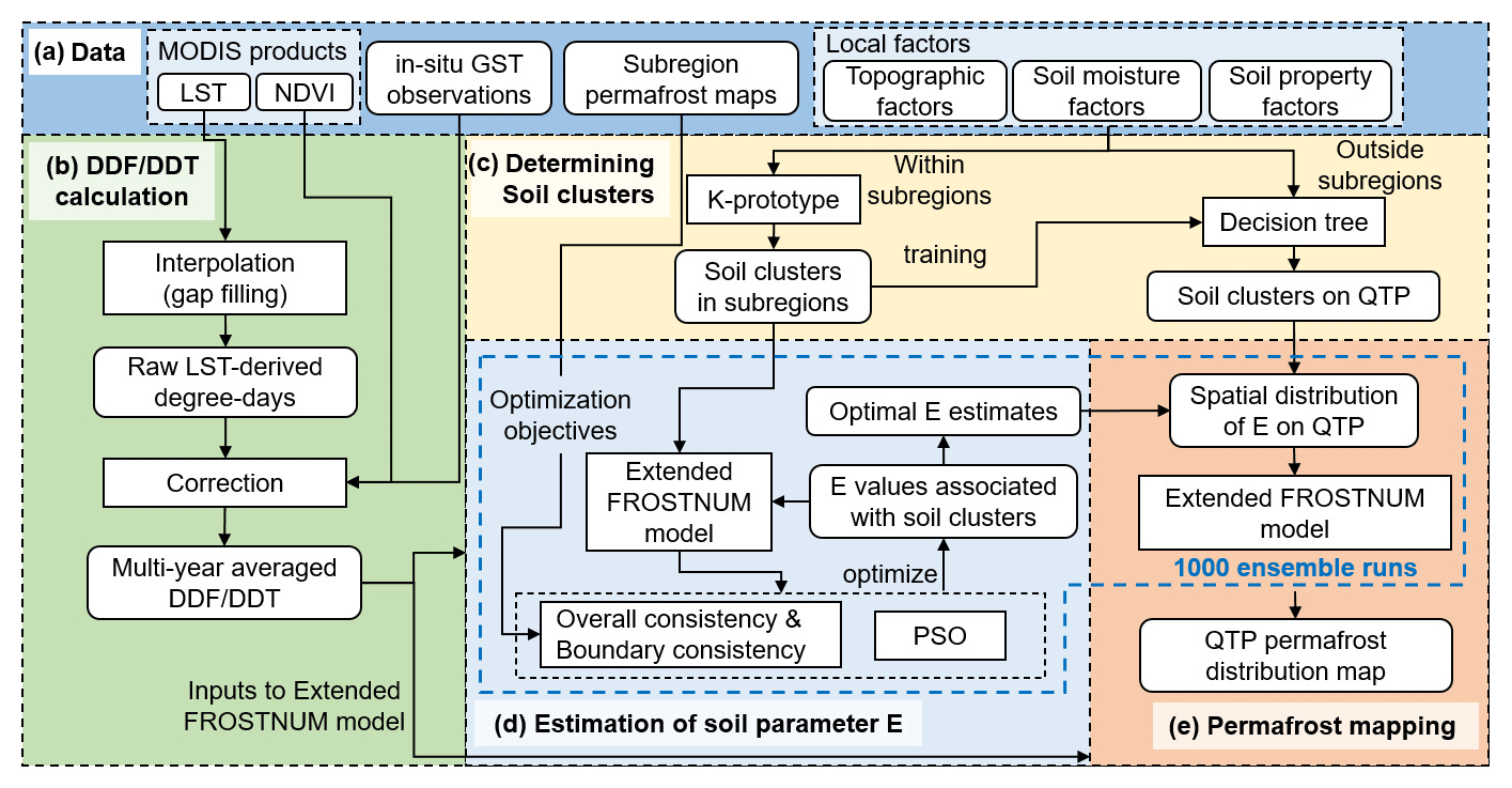
Figure 2Workflow of the permafrost mapping method. Panel (a) outlines the data required in this study. Panel (b) describes the preparation of annual ground surface freezing indices (DDF) and thawing indices (DDT) based on satellite land surface temperature (LST) data. Panel (c) presents the process of spatial clustering of soils in subregions and prediction of clusters for the study area based on local factors. Panel (d) outlines the determination of optimal values for soil parameter E in the model using the particle swarm optimization (PSO) algorithm constrained by the subregion maps. Panel (e) shows the process of mapping the permafrost distribution on the QTP based on 1000 runs using the extended ground surface frost number model (FROSTNUM). Dashed blue lines mark the improved processes over the original FROSTNUM/COP method (Hu et al., 2020), including refinement of the optimization objective and ensemble runs. The diagram was modified from Hu et al. (2020). GST represents ground surface temperature and NDVI is the normalized difference vegetation index.
3.2 Preparation of ground surface freezing and thawing indices
DDF and DDT were calculated based on the MOD11A1 and MYD11A1 Level 3 products (Version 6). Gaps in the MODIS LST data due to cloudiness resulted in systematic cold biases (Westermann et al., 2012) and, consequently, uncertainties in mapping permafrost based on these data. Despite many all-weather LST products (Zhang et al., 2021; Xu and Cheng, 2021), we chose a stepwise interpolation approach based on the solar–cloud–satellite geometry (SCSG) effect (Chen et al., 2023) to interpolate the data-gap regions in the MODIS LST data. Compared with existing approaches, the SCSG-based approach requires only MODIS-family data and is effective for extensive missing data (e.g., on the QTP). A brief introduction to this interpolation method is provided in Appendix A.
Due to the buffering effect of seasonal snow cover and vegetation, thermal offsets often exist between satellite-derived LST values and GST values. In most areas of the QTP, snow cover is thin and short-lived (Wu and Zhang, 2008; Zhao et al., 2017); thus, the buffer effect of snow cover is limited and LSTs are close to GSTs during snow-free periods (Hachem et al., 2012), as also shown later in this study. Therefore, for the DDF values, we simply calculated the sum of negative degree-days of mean daily LST from four instantaneous LST observations, ignoring the effects of snow cover.
Conversely, vegetation cover affects DDT by providing a strong thermal buffer between GST and LST, especially on the eastern QTP during growing seasons. Hence, thermal offsets should be removed from the raw LST data before DDT can be derived as a sum of positive degree-days of mean daily LST. To this end, we developed a multilinear regression model where GST is a function of independent variables including the raw LST, NDVI, and latitude at weather stations (Huang et al., 2020). The correction was repeated over 23 time intervals a year, and the annual DDT was the aggregate of all these corrected positive degree-days. More information regarding this process can be found in Appendix B.
3.3 Determination of optimal values of soil parameter E
We followed the method developed by Hu et al. (2020) to spatially group the soils of five subregions into soil clusters. Because the QTP is a much larger region with more complex climate and terrain conditions than the experimental area in the previous study (Hu et al., 2020), the environmental variables that we chose to account for the influences of local factors on permafrost distribution were slightly different. Apart from the previous factors of elevation, slope, TWI, precipitation, and soil texture type, we added NDVI and FSC as a response to the relatively strong heterogeneity of surface conditions on the QTP. Compared with Hu et al. (2020), we excluded the relief degree due to its high correlation with slope. To enable mixed clustering of both categorical (soil texture type) and numerical variables, the k-prototype approach (Huang, 1998) was employed. Lakes were excluded during the clustering analysis.
The particle swarm optimization (PSO) algorithm (Wang et al., 2018) was used to find the optimal value of E associated with each soil cluster. In this population-based heuristic method, the candidate solutions are guided toward the best-known positions in the search space, thus enabling a very rapid convergence to an optimal value. In the previous study (Hu et al., 2020), the only objective function was Cohen's kappa coefficient (Cohen, 1960), which quantifies the agreement between the simulation map and the survey-based subregion permafrost distribution maps. Despite the good performance achieved in the experimental study area (Gaize in Fig. 1), this relatively simple objective function inevitably leads to equifinality in larger regions such as the QTP. Recognizing that the kappa coefficient is a good representation of the overall consistency between simulation results and subregion maps, we retained the kappa coefficient (κ) and made the objective function more rigorous by adding a specially defined boundary consistency. The objective function is then a weighted sum of overall consistency (κ) and boundary consistency (β):
where Fob is the objective function value, and ωκ and ωβ are the weights imposed on κ and β, respectively (). To minimize the effects of the weights, a random value between 0.2 and 0.5 was chosen for ωβ and, correspondingly, for ωβ in each of a total of 1000 ensemble runs. β represents boundary consistency, which measures how well the boundaries between permafrost and SFG zones in the subregion maps are represented by the simulation.
β is defined as the number of “positive boundary cells” (Nm) normalized by the total number of “boundary cells” (Nb), with a range of 0 to 1:
A boundary cell is a cell on the survey-based subregion maps whose neighboring cells of a size n×n satisfy two conditions: first, the neighboring cells must contain both types of frozen ground (permafrost and SFG); second, the neighboring cells contain at least two soil clusters. According to Eq. (1), the permafrost cells must have larger F values than those of SFG grid cells. Therefore, in the neighboring cells of any boundary cell, the F value averaged over the permafrost zone () must be greater than that of the SFG zone (). A boundary cell is “positive” when this condition () is met, otherwise it is “negative”.
The optimization procedure aims to maximize β as part of the objective function, i.e., as high as possible boundary consistency of the simulated map relevant to the subregion maps. As the DDTs and DDFs were already predetermined in the simulated map before the optimization procedure, the frost number F in each grid cell depends on the E value associated with the specific soil cluster of that cell. This means that, by adjusting the E values of the soil clusters in the neighboring cells of a “negative boundary cell”, the cell has the potential to turn into a positive cell. In the other words, the number of positive boundary cells, or β, is a function of E, thus permitting parametric optimization. To illustrate this concept, we present a simple instance of a boundary cell in Appendix C.
The lower and upper limits of E values were specified at 0.5 and 1.5, respectively, and the optimal E values were determined for all soil clusters occurring in the subregions. Finally, a C5.0 decision tree (Kuhn and Johnson, 2013) was trained on the information of soil clusters in the subregions and then applied to predict soil clusters for all regions outside the subregions on the QTP on a cell basis, based on the same environmental factors used in spatial clustering. After the distribution map of soil clusters on the QTP was obtained, the values of soil parameter E for the QTP were determined by simply looking up the optimal E value associated with each soil cluster in the soil cluster distribution map.
3.4 Mapping permafrost distribution and evaluation
Once E values are known for all QTP cells, the extended FROSTNUM model was run to determine the type of frozen ground of each cell using a threshold of F=0.5, and the permafrost distribution on the QTP could then be mapped. However, this map may still be affected by local optima. To reduce these issues, parameter optimization was performed 1000 times, a number that warranted minimal variability in individual E values in our experiment, and the permafrost distribution on the QTP was estimated 1000 times in response to 1000 different sets of E values. Finally, an ensemble permafrost map on the QTP was generated by majority voting of the 1000 estimates.
We validated the resulting map (hereafter referred to as our map) from multiple aspects. Although these survey-based subregion permafrost maps have been used as constraints during the optimization process, the optimal E values were obtained from all subregion maps as a whole. Therefore, the survey-based permafrost map in each subregion is still of value for validation. We also validated the maps using in situ permafrost presence/absence observations around 2010. We compared our map with two existing permafrost maps, the Zou map and the Wang map, using the same references. In particular, we analyzed the spatial inconsistency between our map and the Zou map in some typical regions. In these regions, we further evaluated the two maps by utilizing additional information from boreholes, satellite imagery, the permafrost zonation index (PZI) map (Cao et al., 2019b), and elevation characteristics. Satellite imagery provides indicative landscape evidence of permafrost occurrence. While the PZI rarely equates to the actual presence of permafrost, it indicates a probability of permafrost presence with a value ranging from 0 to 1 (Gruber, 2012). In some regions of the QTP where permafrost is thermally controlled by elevation, the dependency of permafrost occurrence on elevation provides useful information for evaluating permafrost distribution maps.
4.1 Ground surface thawing and freezing indices
Figure 3 illustrates the comparison between average annual in situ DDT (DDF) values, calculated as averages over 2005–2010 from daily mean GSTs at 131 weather stations on the QTP, and the average annual satellite DDT (DDF) values at the corresponding MODIS pixels derived directly from daily mean MODIS LSTs. The raw LST-derived DDF values exhibited a perfect match with the in situ DDF values, echoing the limited effects of thin and short-duration snow cover on the thermal states of underlying soils on the QTP (Wu and Zhang, 2008; Zhao et al., 2017). In contrast, a notable discrepancy emerged in the LST-derived annual DDT, which tended to underestimate the in situ DDT, resulting in significant deviations at certain sites. The discrepancies are mainly connected to the thermal offset between remotely sensed LST and GST, which has also been reported by previous studies (Luo et al., 2018; Obu et al., 2019).
Obvious negative biases were observed in the raw LST-derived DDT values (Fig. 4a). However, after applying the interval-based approach, the negative biases were well removed. Moreover, the corrected data points were concentrated along the 1:1 line (as shown in Fig. 4b), while the coefficient of determination (R-squared) increased from 0.74 to 0.89. More importantly, the mean absolute error (MAE) value (334 ∘C d−1) of the corrected LST-derived DDTs was about one-third of the value (889 ∘C d−1) before the correction, i.e., the relative error dropped from 23.3 % to 8.8 %, below our accepted level of 10 %. In addition, raw DDT data points with large deviations have been effectively corrected, resulting in a reduction in the root-mean-square error (RMSE) from 1072 to 421 ∘C d−1 after correction. Most corrected data points fall into the ±400 ∘C d−1 band (about 10 %), indicating a well-controlled level of error after the removal of thermal offsets between GST and LST.
The distributions of annual DDT and DDF (Fig. 5a, b) were in close agreement with the characteristics of elevation (Fig. 1), which is one of the main factors controlling ground temperature distribution over the QTP. In general, annual DDT decreased and annual DDF increased with rising elevation. Over the relatively flat high plain between 33–37∘ N and 80–90∘ E, the annual DDT showed moderate latitudinal zonality, declining with increasing latitude, whereas the annual DDF showed the opposite. This is an indication of the influence of solar radiation on GST. The vast area and complex topography of the QTP resulted in a wide spectrum of annual DDT (from 0 to 9000 ∘C d−1) and DDF (from 0 to 8000 ∘C d−1). Most regions of the QTP lie between 3000 and 5500 m a.s.l., where DDT and DDF values were mostly between 1000 and 2500 ∘C d−1. High DDT values appeared in the low mountains in the southeastern QTP, in the Qaidam Basin in the north, and in the southern valleys, whereas high DDF values appeared on the Qiangtang Plateau in the northern QTP and in the high-mountain areas, favoring the formation of permafrost. The DDT / DDF ratio indicates climatic controls on permafrost preservation (Fig. 5c). Regions with a DDT / DDF ratio <1 would have the potential to form permafrost in absence of local factors that affect permafrost formation.
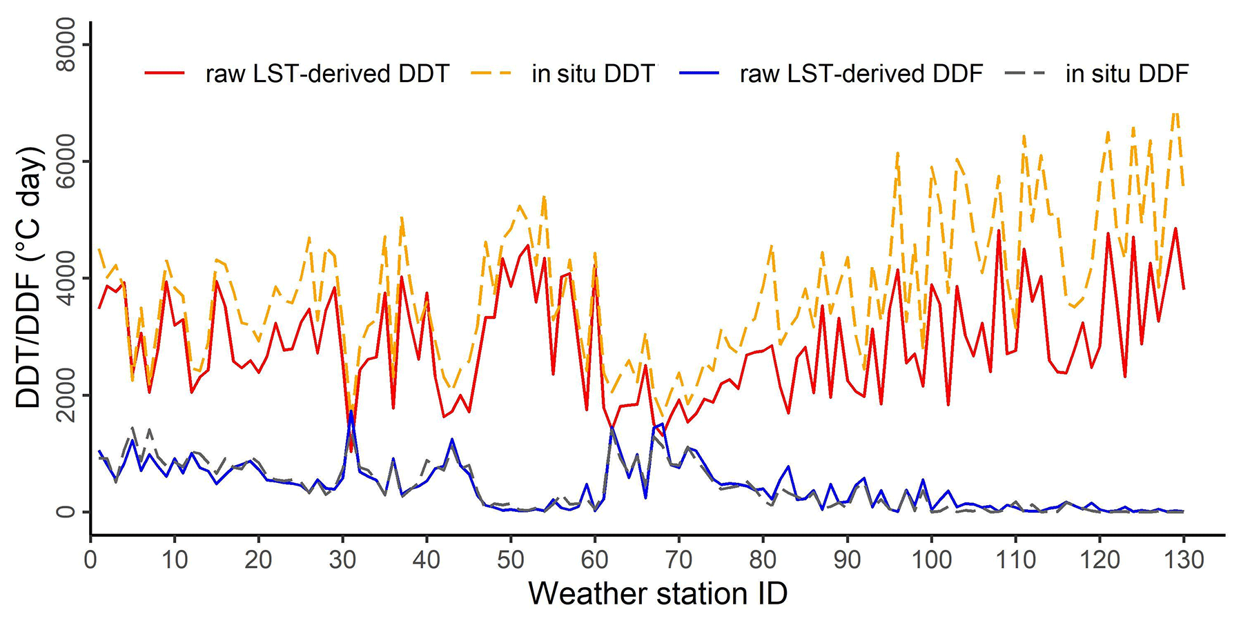
Figure 3Thawing/freezing indices calculated from the interpolated MODIS LST data (raw LST-derived DDT/DDF) and in situ observations of ground surface temperature (in situ DDT/DDF) at each QTP weather station. The ordinate indicates the annual thawing/freezing indices averaged over the period from 2005 to 2010, and the abscissa shows 131 weather stations available on the QTP.
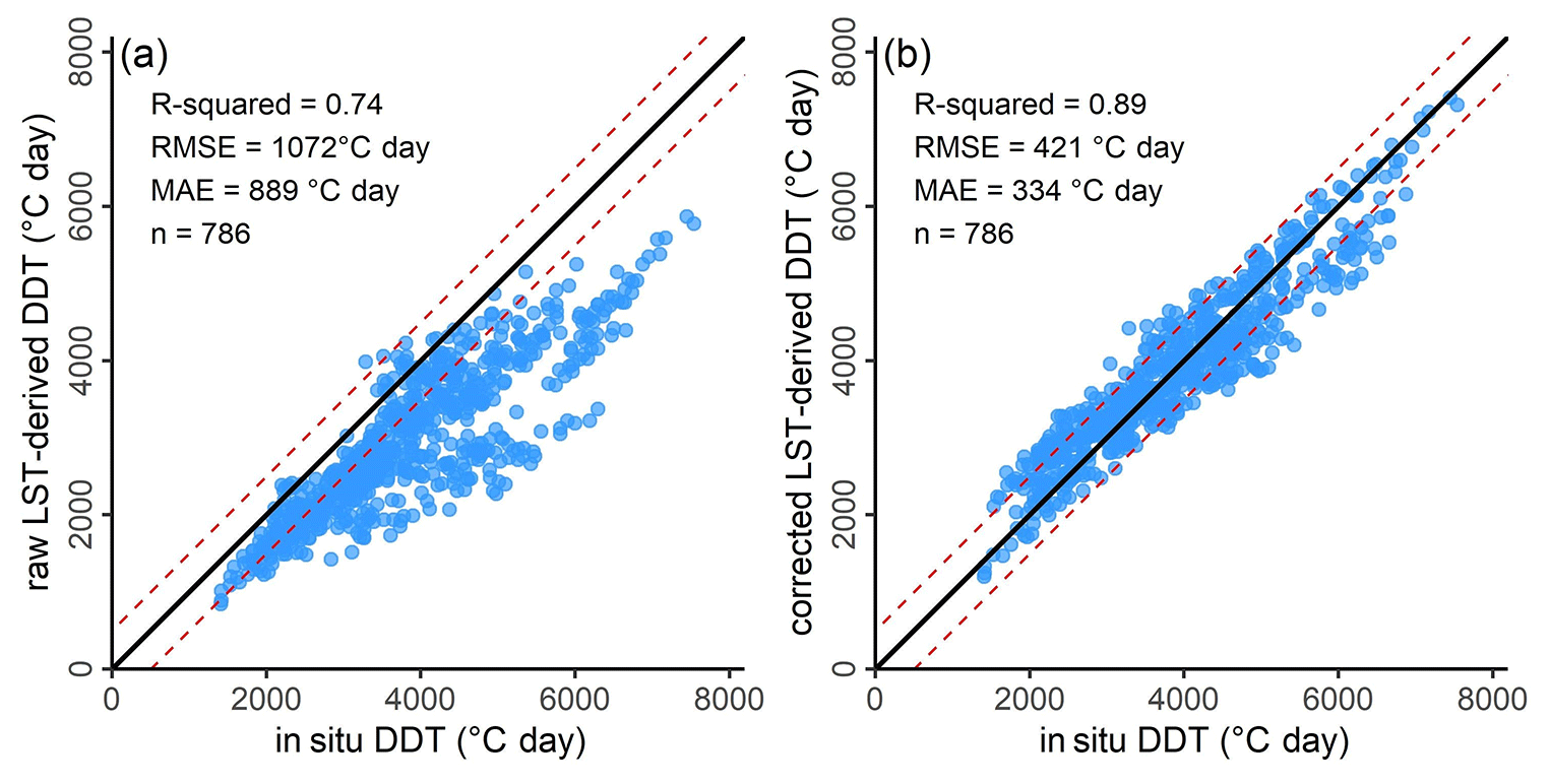
Figure 4Bias correction of MODIS LST-derived DDT with the interval-based approach. Panel (a) presents the data before bias correction, and panel (b) shows the data after applying the interval-based method. Data points represent annual DDT values in 2005–2010 from the 131 stations. The dashed red lines outline a range of ∼10 % (±400 ∘C d−1) from the 1:1 line (solid black line).
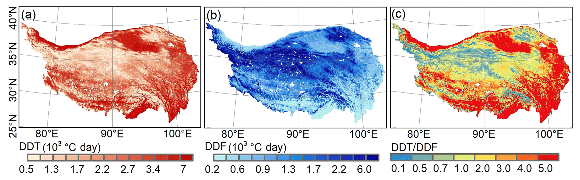
Figure 5Maps of the spatial distribution of (a) annual DDT, (b) annual DDF, and (c) the DDT / DDF ratio on the QTP, averaged over 2005 to 2010. Lakes were excluded and are shown in white, whereas glaciers were included. Regions with a DDT / DDF ratio <1 are climatically favorable for permafrost formation.
4.2 Soil clusters
A total of eight soil clusters were determined by the k-prototype approach in the five subregions (Fig. 6), where lakes were excluded. Soils in one cluster share more similar environmental characteristics with each other, as reflected by a single value of model parameter E, than soils in other clusters. The dominant soil clusters in each subregion differed from each other (Table 1): clusters 3 (30 %) and 1 (30 %) were dominant in West Kunlun, clusters 2 (58 %) and 7 (23 %) were dominant in Gaize, clusters 7 (49 %) and 1 (23 %) were dominant in Aerjin, clusters 8 (55 %) and 7 (18 %) were dominant in G108, and cluster 8 (85 %) was dominant in Wenquan. This implies distinctions between climatic and geographic conditions in these subregions.
Among all clusters, clusters 1, 2, and 3 differ with respect to slope and TWI, but they are all characterized by relatively high elevation (about 5000 m), low vegetation cover (NDVI <0.2), thin snow cover (FSC <10), and aridity (precipitation <200 mm) (Fig. 7), which generally may represent high plateaus. Cluster 4, with the highest TWI, represents the valley with low elevation and moderate slope. Cluster 5 has the highest elevation, highest FSC, and lowest NDVI (even below 0); thus, it may represent high mountains covered by thick snow cover or glaciers. Cluster 6 has very varied elevations and steep slopes, and it occurs on the hillslopes of high mountains. Except for the much lower TWI, cluster 7 is similar to cluster 4, and it often appears around cluster 4, which represents valleys (Fig. 6). Therefore, it is likely that cluster 7 represents gentle slopes near valleys. Cluster 8 is mainly distributed in the two subregions (G308 and Wenquan) on the east QTP; is characterized by the highest NDVI, highest precipitation, and lowest elevation; and represents the soils with better hydrological, thermal, and vegetation conditions on the eastern QTP.
The distribution of soil clusters on the QTP (Fig. 6) was predicted by the decision tree method. Soil cluster 8 covered the largest area of about 37.76 % of the QTP and was mainly distributed in the eastern QTP, which is related to the training samples that were mainly located in G308 and Wenquan on the eastern QTP (Table 1). Soil clusters 2, 3, 6, and 7 covered roughly the same proportion of area, about 10 % of the whole QTP, followed by clusters 1 (6.94 %) and 4 (6.20 %). Soil cluster 5, representing glaciers and regions with thick snow cover, occupied the least area (2.85 %), which is consistent with a previous study that thick snow coverage only represented a relatively small portion of the QTP (Dai et al., 2018).
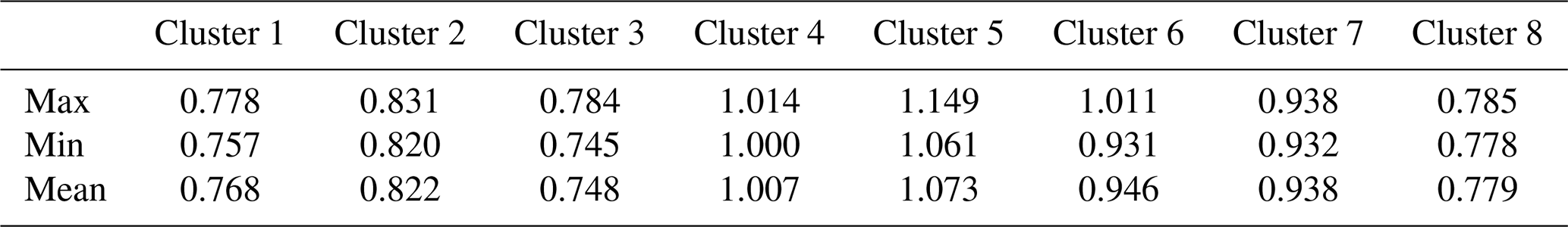
The optimal values of parameter E associated with the soil clusters (Table 2) were determined from the 1000 optimization runs. The ranges of the optimal values were relatively narrow for all soil clusters, suggesting that equifinality was well mitigated due to a well-constrained objective. The mean values as the optima for clusters 4 and 5 were greater than 1, with an implication of unfavorable local conditions for permafrost formation and preservation. For example, heat advection by water flows occurring near rivers in valley areas represented by cluster 4 and the insulation effect of snow cover in regions of cluster 5 are not beneficial for permafrost formation and preservation. Clusters 1, 3, and 8 had relatively lower E values, suggesting favorable local environments for permafrost formation in these regions. Some characteristics of local factors, such as high elevation for clusters 1 and 3 and high precipitation for cluster 8, are beneficial for permafrost preservation (Zhang et al., 2021b), as also reflected by their lower E values.

Figure 6Resulting soil clusters in the five subregions and the predicted distribution of clusters on the QTP. A total of eight clusters were determined. Each soil cluster represents unique traits as reflected by a distinct value of model parameter E.
Table 1Area percentages occupied by individual soil clusters in each subregion, over all subregions, and over the entire QTP.
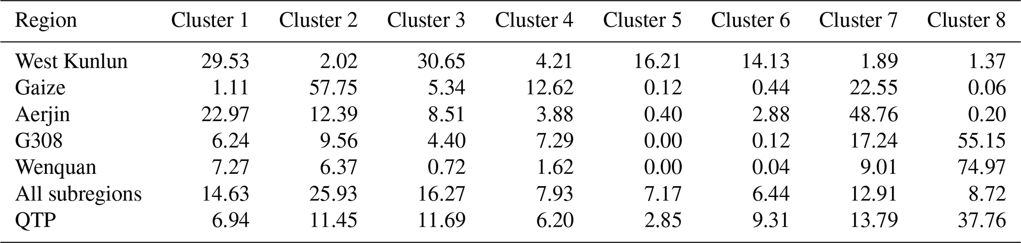
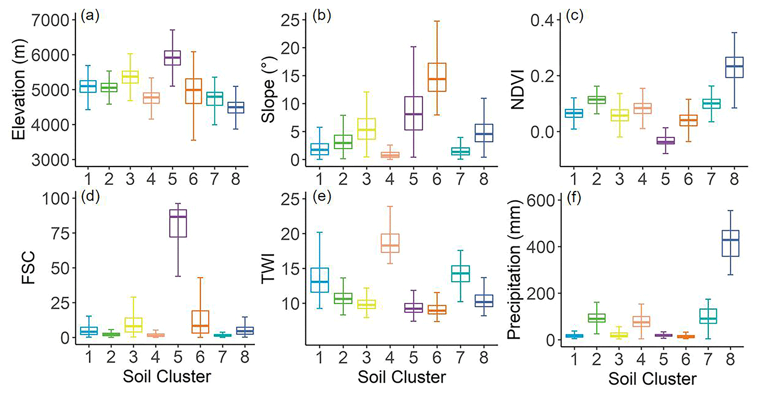
Figure 7Soil clusters' environmental characteristics in the subregions: (a) elevation, (b) slope, (c) normalized difference vegetation index (NDVI), (d) fractional snow cover (FSC), (e) topographic wetness index (TWI), and (f) precipitation. All clusters are shown in different colors to match those in Fig. 6. The center line in the box shows the median, the box shows the lower and upper quartiles, and the whiskers extend to the minimum and maximum data values.
Table 2Ranges and mean values as the most optimal values of the soil parameter E associated with the eight soil clusters. The results were obtained from 1000 optimization trials.
4.3 The resulting 2010 permafrost distribution map on the QTP
The resulting permafrost distribution in 2010 on the QTP is shown in Fig. 8 with a spatial resolution of 1 km. Permafrost covered about 1.086×10⁶ km2, or 41.17 %, of the QTP, while SFG occupied about 1.447×10⁶ km2, or 54.85 %, of the total QTP area. The non-frozen ground was about 2.24×10⁴ km2 (0.85 % of the QTP), and the rest consisted of glaciers (about 4.08×10⁴ km2, or 1.55 %) and lakes (about 4.17×10⁴ km2, or 1.58 %).
The map shows that permafrost was prevalent throughout the northern central QTP, especially on the Qiangtang Plateau. In the north, the Qaidam Basin was occupied by SFG due to its low altitude, interrupting the continuity of permafrost that extended north to the Qilian Mountains. From the central Qiangtang Plateau southward, the spatial continuity of permafrost tended to decline due to decreasing latitude and elevation. Near the permafrost zone in the Bayan Har Mountains and Tanggula Mountains in the eastern QTP, SFG occurred extensively in the river source areas, namely the Three-River Headwaters Region, probably due to the low latitude and the effects of heat advection by water flows that prevent permafrost formation. As the DDT / DDF ratios in these regions were generally greater than 1 (Fig. 5c), permafrost in the river source areas (e.g., the Yangtze River headwaters) was thermally vulnerable and very sensitive to climate warming (Zhang et al., 2022). On the southern QTP, permafrost was sporadically distributed at high elevations, mainly in the high mountains of the Eastern Himalayan Syntaxis, the Gangdise Mountains, and the Himalayan Mountains. Only a small amount of non-frozen ground existed in the southern QTP.
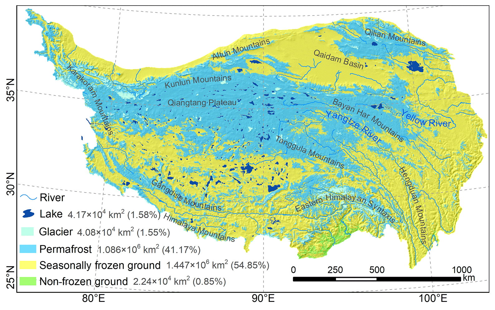
Figure 8Map of permafrost distribution at a 1 km resolution over the QTP in 2010 (our map) produced in this study. Areas and percentages of frozen soil types are provided. The map shows hillshading with elevation.
4.4 Assessment based on survey maps and borehole data
Our map showed substantial spatial agreement with the survey-based permafrost maps in all subregions (Fig. 9). Our map had a Cohen's kappa coefficient (κ) of about 0.74 (Table 3), which was notably higher than that of the Zou map and the Wang map, which were 0.55 and 0.50, respectively. Overall, compared with the survey-based maps (Fig. 9a) and our map (Fig. 9b), the Zou map significantly overestimated permafrost extents in Gaize and Aerjin and underestimated permafrost extent in G308 (Fig. 9c), whereas the Wang map severely overestimated permafrost extents in all subregions (Fig. 9d). The differences can be better discerned in the difference maps in Fig. E1.
More specifically, in permafrost-dominated West Kunlun, our map and the Zou map slightly overestimated the extent of the SFG around the lake, whereas the Wang map slightly underestimated the extent of SFG. There were only small differences between the three maps in West Kunlun, with almost the same κ for all three maps (0.62 for our map and 0.63 for both the Zou map and the Wang map). All three maps were based on satellite LST data, which can generally capture the patterns of surface ground temperature. Although the interpolation methods for processing LST gaps differed and resulted in data with different accuracy for mapping, the cold climate in West Kunlun, with LST values well below 0 ∘C in most areas, made the impact of these differences in input data on permafrost distribution negligible.
In Gaize, our map performed better (κ=0.71) than the Zou map (κ=0.48) and the Wang map (κ=0.43). Both the Zou and Wang maps severely overestimated permafrost distribution, whereas our map agreed well with the survey-based map in this region (Fig. 9b). The same trends occurred in Aerjin, and the comparison with the survey-based map indicated a much lower κ for the Zou map (0.38) and the Wang map (0.00) than for our map (0.71). Gaize has a warmer climate than West Kunlun and contains the southern limit of continuous permafrost. Therefore, the influence of input data accuracy and local factors on permafrost preservation is more profound in this area. The overestimated permafrost extents in Gaize and Aerjin in both the Zou map and the Wang map may most likely be related to the relatively lower quality of the interpolated LST data as model input and insufficient consideration of local factors in the mapping approaches. Compared with the harmonic analysis of time series (HANTS) algorithm (Xu et al., 2013) used for the Zou and Wang maps to reconstruct the missing LST data under clear-sky assumptions, the SCSG-based interpolation method with full consideration of cloud effects on LST used in this study was found to be effective for handling large areas of missing data with sufficient accuracy (Chen et al., 2023). Moreover, the daily GST data required to produce the Zou and Wang maps were the weighted sum of four MODIS LST observations per day through an empirical linear formula based on sample observations from three automatic weather stations in the central QTP (Zou et al., 2014). This relatively simple treatment of GST data in the Zou and Wang maps can lead to considerable systematic biases in some regions, especially in warm permafrost regions (e.g., the Gaize subregion) that are highly vulnerable to thermal perturbations like persistent regional climatic warming (Zhang et al., 2021a), and ultimately cause large uncertainties in the final permafrost distribution maps. In contrast, the thermal offsets between GST and LST have been well handled in this study when estimating thawing indices from satellite LST observations by considering the effect of vegetation cover as a buffer layer based on 131 weather stations over the QTP. As the Wang map was produced using statistical learning methods, uncertainties also resulted from training samples selected from two previous QTP permafrost maps produced in different years more than a decade apart and subject to varying levels of uncertainty (Ran et al., 2012; Zou et al., 2017). Together, all of these factors caused the Wang map to overestimate the permafrost extent in Gaize.
In G308, the Wang map (κ=0.68) indicated more permafrost areas than the local survey map, whereas both the Zou map (κ=0.48) and our map (κ=0.68) showed fewer permafrost areas compared with the local survey map, with the Zou map even more evident. The soil thermal regime in G308 is strongly influenced by rivers and vegetation cover; these effects were well accounted for in our mapping approach, whereas they were absent in the Zou map. In Wenquan, both our map (κ=0.70) and the Zou map (κ=0.65) performed generally satisfactorily, with a slight overestimation of permafrost extent. In contrast, the overestimation was more pronounced in the Wang map (κ=0.46), which is probably also related to the misrepresented training samples used for this map.
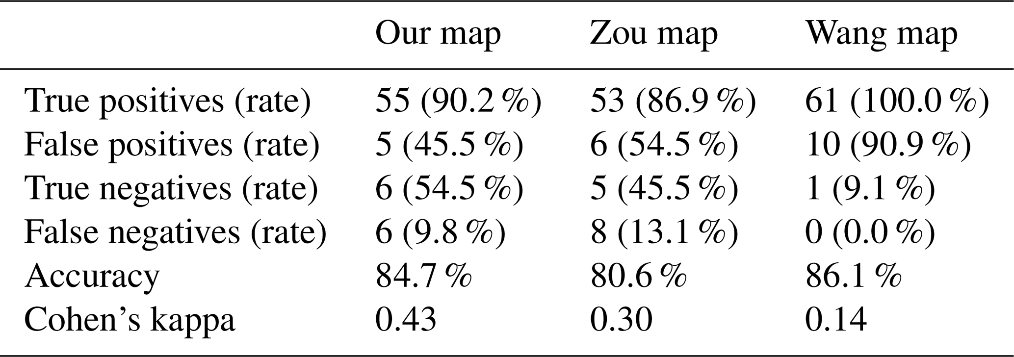
The maps were also verified by 72 permafrost presence/absence observations obtained by boreholes drilled within a 5-year time frame around 2010 (Li et al., 2016; Zhao et al., 2021). Only our map showed good agreement (κ=0.43) with the borehole observations in terms of κ (Table 4), compared with the Zou map (κ=0.30) and the Wang map (κ=0.14). According to the borehole observations, SFG was underrepresented in all three maps, with our map performing the best with respect to predicting SFG (with 54.5 % accuracy), as opposed to the Wang map that showed the worst performance (correctly identifying only 1 out of 11 seasonal frost boreholes). Unlike SFG, permafrost was overestimated at borehole locations in three maps, as evidenced by relatively high false-positive (permafrost) rates (45.5 % for our map, 54.5 % for the Zou map, and 90.9 % for the Wang map). As most of the borehole locations were underlain by permafrost (Fig. 9), the Wang map predicted almost all locations as permafrost with no discretion, as indicated by a 100 % true-position rate (Table 4), and consequently led to an inflated accuracy of 86.1 %, which was the highest among the three maps.
In our map, two out of six false negatives (misidentified as SFG) were the boreholes with unstable permafrost located in the SFG zone close to the permafrost boundary. However, in the Zou map, all eight false negatives were boreholes with stable permafrost, and those with unstable permafrost were in the permafrost zone. If we excluded all four boreholes with unstable permafrost from the evaluation, the false-negative rate of our map would drop from 9.8 % to 7 % and κ would rise from 0.43 to 0.49, whereas the false-negative rate and κ of the Zou map would remain almost unchanged, leaving an even higher false-negative rate (∼13 %) than that of our map (∼7 %). This borehole-based verification may be biased by the mismatch between a site and a 1 km ×1 km grid cell. Nevertheless, considering the collective evidence, our map demonstrates satisfactory performance with respect to predicting frozen ground distribution.
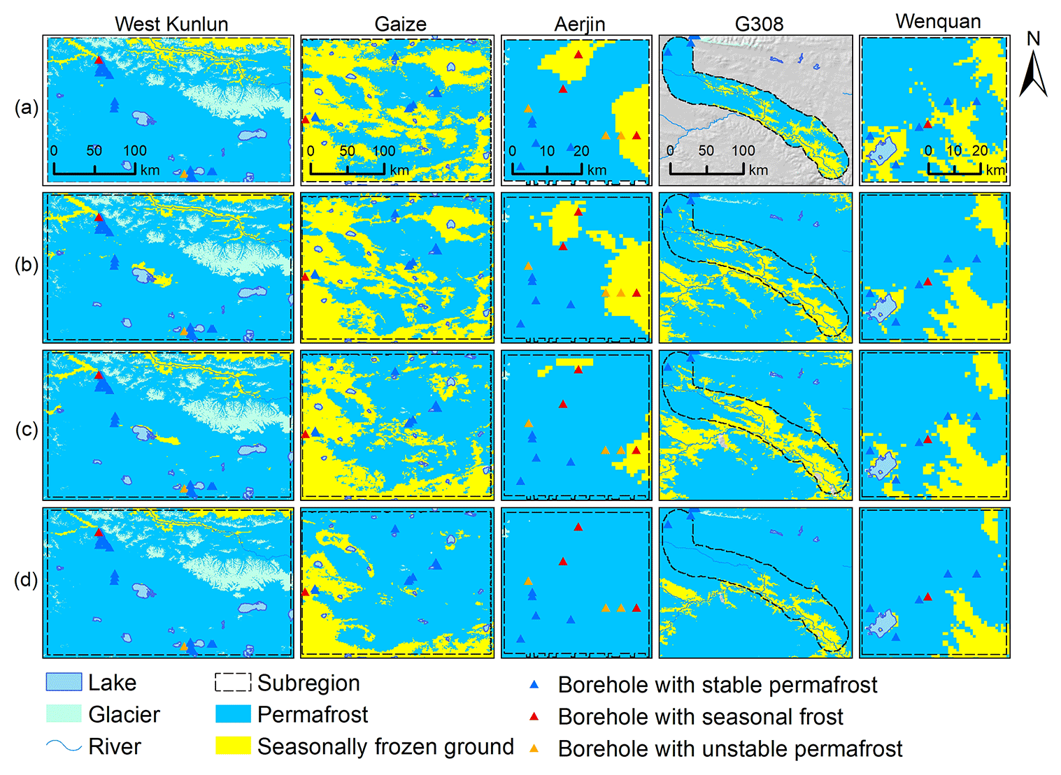
Figure 9Spatial distributions of frozen ground in the subregions from (a) survey-based maps, (b) our map, (c) the map from Zou et al. (2017), and (d) the map from Wang et al. (2019). Triangle symbols mark the locations of boreholes drilled in around 2010. Difference maps between survey-based maps and the three simulated maps are provided in Fig. E1.
Table 3Kappa values measured between the evaluated permafrost maps (our map, the Zou map, and the Wang map) and survey-based maps in the subregions.
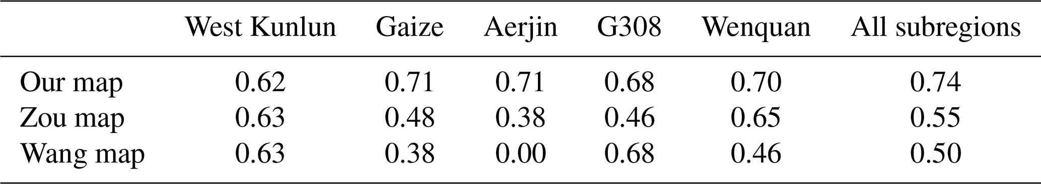
Table 4Measures of confusion matrices describing the performance of the evaluated permafrost maps (our map, the Zou map, and the Wang map) at the borehole locations. To fit the binary classification, permafrost is regarded as positive and SFG is considered negative. n=72.
4.5 Cross-comparison with the Zou map
The permafrost distributions in our map and the Zou map were generally comparable, although there were discrepancies in some regions (Fig. 10), mainly in the transition region between the continuous permafrost zone of the Qiangtang Plateau to the north and the SFG zone to the south. In addition, the headwaters of China's major rivers (regions c and d in Fig. 10) in the eastern QTP showed noticeable spatial inconsistency between the two maps. These headwater regions were reported to be the critical regions where permafrost is warm and very susceptible to degradation due to climate change (Jin et al., 2011; Zhang et al., 2021a). Permafrost there is characterized by high temperature (MAGT ∘C) and low thermal stability (Qin et al., 2017). The warm permafrost is difficult to distinguish from SFG, which poses a challenge to the accuracy of soil temperature modeling. Moreover, permafrost in transition areas is often controlled by many local factors (e.g., terrain, vegetation cover, soil properties, and hydrological conditions), and a model without adequate consideration of local factors often fails to accurately describe the soil thermal regime.
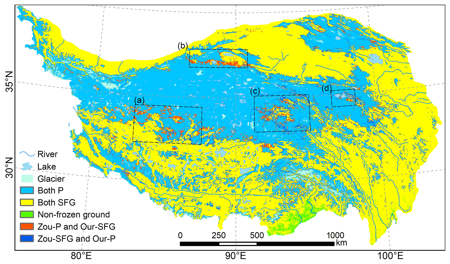
Figure 10Spatial inconsistencies in the distribution of frozen ground between our map and the Zou map. “Both P” represents areas identified as underlying permafrost in both maps, “Both SFG” represents areas identified as seasonally frozen ground (SFG) in both maps, “Zou-P and Our-SFG” represents areas identified as underlying permafrost in the Zou map but SFG in our map, and “Zou-SFG and Our-P” represents areas identified as SFG in the Zou map but permafrost in our map. The dashed boxes highlight areas of significant inconsistency: (a) Gaize and its vicinity, (b) the areas between the Altun Mountains and the Kunlun Mountains, (c) the headwaters of the Yangtze River, and (d) the headwaters of the Yellow River.
In and around Gaize (region a in Fig. 10), a larger extent of permafrost was simulated in the Zou map than in our map. Comparisons of the two maps with the survey-based Gaize map (Fig. 9) have already confirmed the better performance of our map in this region than the Zou map, due to the use of the survey-based Gaize map as part of the constraints in modeling our map (Table 3). The vicinity of Gaize is very similar to the Gaize subregion, also characterized by a relatively flat plateau with an arid climate and low vegetation cover. It can be inferred that our map could likely have better accuracy than the Zou map in and around the Gaize subregion.
In the areas between the Altun Mountains and Kunlun Mountains (region b in Figs. 10 and 11) containing the Aerjin subregion, our map estimated much more SFG than the Zou map. Referring to the survey-based Aerjin subregion map (Fig. 9), the Zou map underestimated the extent of SFG, and our map showed a better performance despite a slight overestimation of SFG extent. According to borehole records (Fig. 9) in the Aerjin subregion, some locations had ground temperatures at 10 m of about −0.1 to 0 ∘C, and one borehole location was even above 0 ∘C but fell within a permafrost zone in the survey-based map. This reflects that permafrost in this region was extremely thermally unstable. We inspected inconsistency zones identified as permafrost in the Zou map but as SFG in our map (Fig. 11a), where the DDT / DDF ratios were around 1.3 (Fig. 11b) and clusters 4 and 7 predominated with E values of about 1.07 and 0.94, respectively (Fig. 6). Those characteristics are very similar to the SFG zone in the survey-based Aerjin map. Following Eq. (1), surface frost numbers were less than 0.5 in these areas with a climatic implication of no permafrost presence. From the satellite image (Fig. 11c), it can be seen that rivers are well developed in the basins. The presence of these rivers could potentially lead to greater degradation of permafrost due to the thermal advection of water flows. Overall, our map showed more acceptable distribution characteristics in this region than the Zou map. However, further field studies are necessary to provide more direct evidence to strengthen our understanding of permafrost distribution in this critical region.
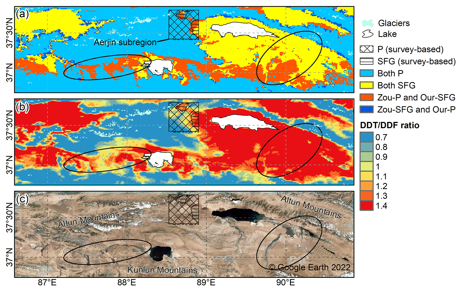
Figure 11Maps of the areas between Altun Mountains and Kunlun Mountains (region b in Fig. 10) showing (a) detailed spatial differences in permafrost distribution between our map and the Zou map, (b) the DDT / DDF ratios, and (c) a satellite image covering this region from Google Earth. The box indicates the Aerjin survey area for which the survey-based permafrost map is available. P (survey based) and SFG (survey based) represent permafrost and seasonally frozen ground in the survey-based map, respectively. The reader is referred to the caption of Fig. 10 for an explanation of the notation used in the legend. Ovals mark areas that were most likely to be thermally affected by the presence of waterbodies.
In the source areas of the Yangtze River (region c in Figs. 10 and 12), the riparian zones were generally identified as SFG in both our map and the Zou map. However, the SFG zones in our map spread on both sides along the rivers, whereas they were distributed on only one side of the rivers in the Zou map. In this region, 35 observations of permafrost presence/absence were collected. Of these, 32 were drilled in 2020 during the Second Tibetan Plateau Scientific Expedition and Research campaign (Li et al., 2022), so they were not included in the quantitative validation above. Boreholes QTB11, QTB15, and TGLGT (Fig. 12), collected from Zhao et al. (2021), were drilled before 2010, and the frozen ground types at these borehole locations were correctly identified in both maps. For the 32 boreholes drilled in 2020, 2 of 6 boreholes with seasonal frost and 24 of 26 boreholes with permafrost were correctly identified in our map, whereas no borehole with seasonal frost and 24 boreholes with permafrost were correctly identified in the Zou map. The misidentified boreholes were located near the boundary of the permafrost zone on our map, whereas they were mostly located within permafrost zones on the Zou map. We also noted that two upstream boreholes at 4870 m (Li et al., 2022), located within a permafrost zone in both maps (red box in Fig. 12a and b), were revealed as seasonal frost in 2020. In a borehole labeled QTB15 (Fig. 12a, b; Zhao et al., 2021) in this region, ground temperature experienced a significant increase from 2006 to 2018 (Table E1), indicating a warming trend. Considering the potential impact of climate warming occurring in this region over the past decade, it is possible that permafrost degradation occurred at the two upstream borehole locations, resulting in the conversion of permafrost in 2010 to SFG in 2020. In these areas, the occurrence of permafrost degradation usually recedes to upstream areas with higher elevations and cooler air temperatures. In other words, by reasonable inference, permafrost would remain in upstream areas in 2010, whereas SFG would be present in downstream areas along the rivers, as well depicted by our map (Fig. 12a).
We further examined the two maps in the Yangtze River source areas using a PZI approach (Cao et al., 2019b). By definition, permafrost regions should have higher PZI values than SFG regions. The PZI map (Fig. 12d) used here was compiled based on 1475 in situ observations (Cao et al., 2019b), many of which were obtained between 2005 and 2018 in the vicinity of the G109 national highway traversing the Yangtze River headwaters, making the PZI map a possible reference in this region. The PZI statistics for permafrost in our map were close to those in the Zou map (Fig. 12e). However, for the PZI statistics in SFG regions, the lower and upper quartiles in the Zou map were 0.36 and 0.66, respectively, whereas the values in our map were 0.34 and 0.53, respectively. The SFG regions shown in our map had lower PZI values. The upper quartile for SFG regions (0.66) in the Zou map surpassed the lower quartile for permafrost regions, which was 0.55. The overlap is questionable because it suggests that some SFG regions have higher PZI values than permafrost regions in the same map, which contradicts the PZI definition. In contrast, the PZI ranges for both frozen ground types were more clearly distinguishable on our map.
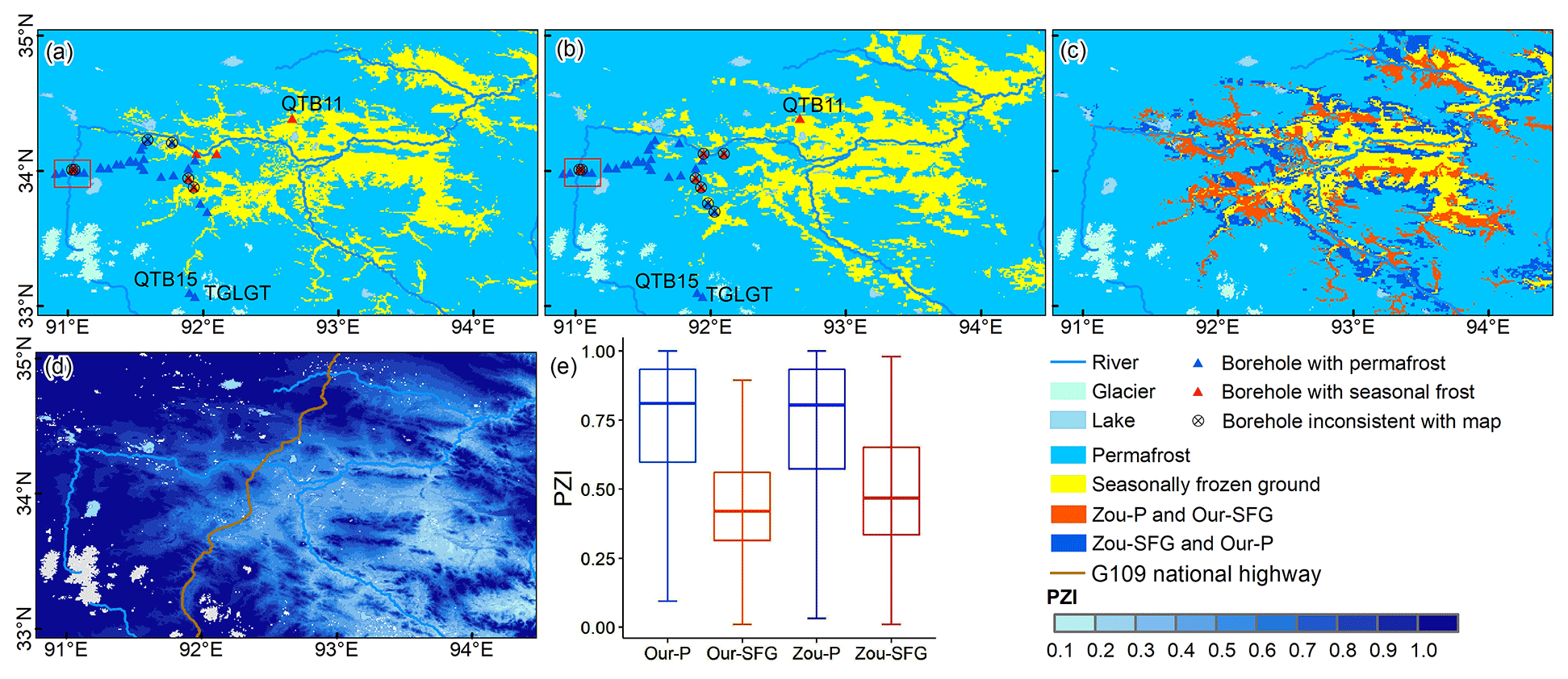
Figure 12Maps of the Yangtze River headwaters (region c in Fig. 10) showing permafrost distributions in (a) our map and (b) the Zou map as well as (c) the spatial differences and (d–e) the spatial and statistical permafrost zonation index (PZI) distributions in this region. The boreholes QTB11, QTB15, and TGLGT in panels (a) and (b) were drilled before 2010 and provided by Zhao et al. (2021), whereas the others were drilled in 2020 during the Second Tibetan Plateau Scientific Expedition and Research program (Li et al., 2022). The red box in panels (a) and (b) covers two boreholes of particular concern. Both boreholes, at an elevation of 4870 m a.s.l., were within a permafrost zone in both our map and the Zou map but revealed seasonal frost in 2020. For panel (c), the same notation applies as outlined in the caption of Fig. 10. Panel (e) presents a box plot of the statistical distributions of PZI values for permafrost and SFG regions on our map (Our-P and Our-SFG) and those on the Zou map (Zou-P and Zou-SFG). The center line in the box shows the median, the box shows the lower and upper quartiles, and the whiskers extend to the minimum and maximum data values.
Similar to the Yangtze River source areas, there were considerable discrepancies between our map and the Zou map in the Yellow River source areas (region d in Figs. 10 and 13). In this region, observations of seven boreholes in 2013 and 2014 collected from Li et al. (2016) were used as independent references. Our map was more accurate, as five of the seven borehole locations were correctly identified in our map, but only three were correctly identified in the Zou map. Considering that elevation is the main factor controlling the permafrost distribution in this region, we conducted an analysis of elevation-related characteristics in this area. According to Li et al. (2016), the lower limit of permafrost occurrence in this region was around 4300 m. Our map showed greater consistency of permafrost distribution conforming to elevational characteristics than the Zou map, and the boundaries of permafrost zones of our map extended along the 4300 m contour in this area (Fig. 13a). In the Zou map, the permafrost area near the two lakes lower than 4300 m a.s.l. was overrepresented (Fig. 13b).
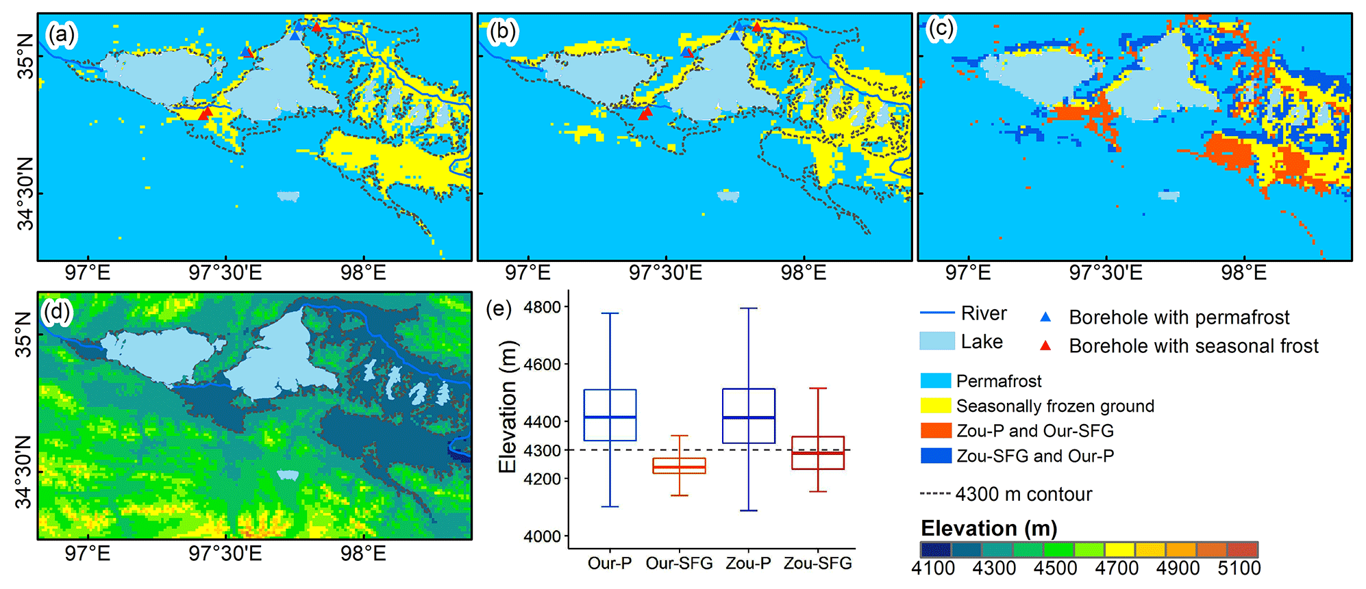
Figure 13Maps of the Yellow River headwaters (region d in Fig. 10) showing permafrost distributions in (a) our map and (b) the Zou map as well as (c) the spatial differences and (d–e) the spatial and statistical elevation distributions in this region. The contour at 4300 m a.s.l., as the lower limit of permafrost occurrence in this region, is shown in panels (a), (b), and (d). Panel (e) presents a box plot of the statistical distribution of elevations in the permafrost and SFG zones in both maps. The same notation applies as that used in Fig. 12.
4.6 Simulation limitations
Despite the better performance of our map compared with other available products, our mapping approach had limitations and left room for potential improvements. We extracted GST observations from weather stations to estimate DDT from LST-derived thawing degree-days. However, GST sites are actually concentrated mainly in the eastern QTP, with few in the west (Fig. 1). This has a detrimental effect on the quality of the DDT estimate. Therefore, we developed multilinear regression models incorporating the NDVI as a predictor. This not only properly reflects the thermal offset due to vegetation cover in the eastern QTP, where weather stations are concentrated, but also helps avoid overfitting in areas of low NDVI (<0.1) in the western QTP, where thermal offset tends to be low. It should also be noted that, although the resulting DDT/DDF values still have some degree of bias, the residual errors were further reduced during the optimization process of our mapping approach by adjusting the E values to best match the simulated results with the survey-based subregion permafrost maps. We also imposed boundary consistency as a part of the more stringent objectives during the optimization process, but the problem of parametric equifinality could not be fully solved and deserves further research, especially when working with binary classification maps (permafrost or SFG).
Our mapping approach relies on subregion survey maps to set up constraints on the simulation and to properly account for the influence of local factors by calibrating a model parameter. The quality and representativeness of subregion survey maps have a strong influence on the accuracy of the resulting permafrost map. In our approach, the heterogeneity of local factors in space is also represented by soil clusters. While more soil clusters can, in theory, better represent spatial heterogeneity, there is a contradiction between the number of soil clusters and the effectiveness of parameter optimization. More soil clusters result in a smaller area for each soil cluster, and a smaller area would lead to a weaker constraint in the search of optimal parameter values, thereby causing a stronger equifinality. Therefore, our mapping approach can benefit from more high-quality subregion permafrost maps, which could provide more soil clusters to better represent the heterogeneous influences of local factors.
The new 2010 permafrost distribution map and associated data (annual DDT and DDF data derived from MODIS LST data and soil clusters over the Qinghai–Tibet Plateau) are available from the repository hosted on Figshare (Cao et al., 2022): https://doi.org/10.6084/m9.figshare.19642362. Data are provided as GeoTIFF files (.tif). The sources of the datasets used for mapping and comparison are listed in Appendix D. The related codes and sample data are accessible at https://github.com/nanzt/frostnumcop (last access: 1 September 2023) (Cao et al., 2023): https://doi.org/10.5281/zenodo.8301453.
This study provides a map of the permafrost distribution over the QTP in 2010 at a spatial resolution of 1 km using a modified version of the FROSTNUM/COP mapping approach. This approach estimated the permafrost distribution using an ensemble run of a semi-physical model based on satellite temperature data and properly accounted for the effects of local factors by adjusting a model parameter constrained by survey-based subregion permafrost maps. Ground surface thawing and freezing indices with a relative error <10 % were obtained from interpolated all-weather MODIS LST data. The problem of parametric equifinality was well mitigated by including boundary consistency as part of the objective function.
According to the new 2010 map, excluding glaciers and lakes, permafrost underlaid about 1.086×10⁶ km2 (41.2 % of the total QTP area) and seasonally frozen ground covered about 1.447×10⁶ km2 (54.9 % of the total QTP area) on the QTP in 2010. Permafrost spread continuously across the Qiangtang Plateau in the northern central QTP. The seasonally frozen ground was mainly distributed in the southern and eastern QTP. Our map also revealed that SFG was widespread in the headwater regions of rivers in the eastern QTP.
This map showed good consistency with the survey-based subregion permafrost maps, with κ=0.74, which is much higher than that of two recently published maps (Zou et al., 2017; Wang et al., 2019c). Upon validation against 72 borehole records of permafrost presence collected around 2010, we concluded that our map performed better than the Zou map and the Wang map. In some regions where we found distinct differences between our map and the Zou map, our map proved more acceptable; this was supported by evidence from various aspects, including satellite imagery, PZI statistics, elevation features, and more independent boreholes records. Our new 2010 permafrost distribution map provides accurate and fundamental information about QTP permafrost and can, thus, serve as a benchmark map to calibrate/validate spatial simulations of land surface models on the QTP as well as a historical reference for projecting future changes in QTP permafrost.
We applied a stepwise interpolation approach to estimate missing cloudy-sky land surface temperature (LST) values of MODIS from informative samples due to the SCSG effect, by which satellite imagery records the cloudy-sky LST values of a portion of pixels. The satellite and Sun have specific illumination and observation angles with respect to the ground. Based on the SCSG effect (Wang et al., 2019a), each MODIS LST image was processed into four SCSG regions, with one SCSG region containing known cloudy-sky LST values. A clear-sky interpolation method with the advantage of effectively handling large data gaps (Chen et al., 2020) was used to estimate clear-sky LST equivalents for every pixel in cloud-affected regions. This method estimated multiple initial estimates for each interpolated pixel by an empirically orthogonal function method based on multiple temporally proximate reference images, and it then merged the initial estimates using a Bayesian approach to obtain a best estimate of the clear-sky LST equivalent. Then, for each missing cloudy-sky pixel, a multivariate adaptive regression splines model (Friedman, 1991) was trained with the pixels in the specific SCSG region with known cloudy-sky LST values that were similar to that missing pixel in terms of environmental characteristics, and then the trained model was applied to recover the missing cloudy-sky LST values (Chen et al., 2023). The fraction of pixels with null values for each image after the interpolation was small and was further interpolated by an ordinary Kriging method. This resulted in four all-weather LST values per day for all 1 km MODIS pixels. A sinusoidal method (Van Doninck et al., 2011) was applied to calculate the daily mean LSTs based on four instantaneous LST observations and the corresponding acquisition times.
Table B1Comparison of performance between two (interval-based and 1-year) approaches of estimating annual DDT from raw LST-derived thawing degree-days based on 100 trials with a random split of the training and test datasets from meteorological sites on the QTP. The values indicate the metric means from the 100 random trials, and the values in parentheses represent ranges. r denotes Pearson's correlation coefficient, RMSE represents the root-mean-square error, and MAE is the mean absolute error.
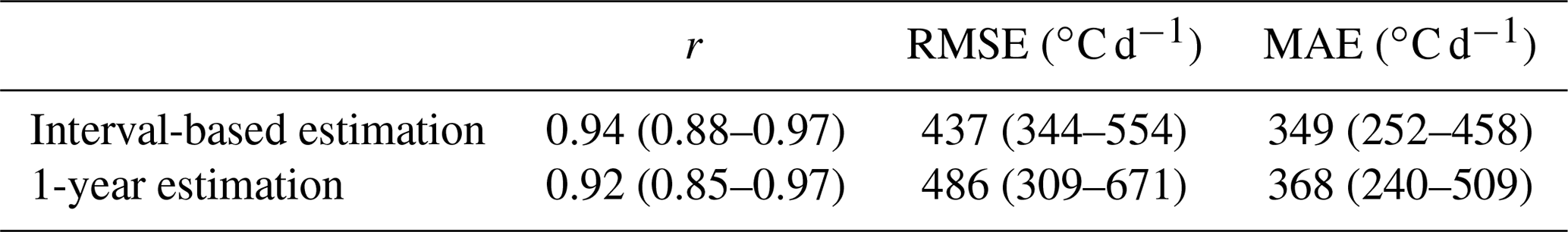
We tested two methods to estimate the annual ground surface thawing index (DDT) from the raw LST-derived thawing degree-days at a MODIS pixel: one is a “1-year estimation”, in which a single regression model was fitted for each year; the other is a form of “interval-based estimation”, in which a full year was divided into 23 time intervals in line with the 16 d composite NDVI intervals each year and multilinear regression was made for each interval. Most intervals consist of 16 d, except for the last interval. The thawing degree-days over the 23 intervals per year were summed for the annual DDT.
The multilinear regression model for each time interval has the following form trained on data at meteorological sites:
where is the ground surface thawing index for the ith interval of the year, is the thawing degree-days derived from the positive daily mean LST values of the pixelfor the ith interval, Ni refers to the ith composite NDVI value of the pixel, and L is the latitude. The index i ranges from 1 to 23. The training was based on meteorological records aggregated from all sites. The fitted functions (f) for individual intervals were then applied to the entire QTP to obtain the corrected interval thawing degree-days of a year, before summing them for the annual DDT for that year. To minimize the risk of single-year meteorological anomalies, annual freezing index (DDF) and DDT values were averaged over the period from 2005 to 2010 and then used to drive the extended FROSTNUM model. The 1-year estimation is on a yearly basis, rather than on an interval basis, following an approach similar to Eq. (B1) but without the need to sum the interval-based values.
To compare the performance of the interval-based estimation method and the 1-year estimation method, we randomly divided the 131 weather stations into a training set (70 %) and a testing set (30 %) 100 times. Each time, we performed both interval-based estimation and 1-year estimation based on the same training set, and we then assessed their prediction results using the testing set. Pearson's correlation coefficient (r), the root-mean-square error (RMSE), and the mean absolute error (MAE) were used as performance metrics.
By carrying out an evaluation using annual in situ DDT values at QTP sites, the annual DDT values obtained by the interval-based estimation had generally lower errors and better linear correlation than the DDT values obtained by the 1-year estimation (Table B1). The ranges of metric values for the interval-based estimation were all narrower than those for the 1-year estimation, indicating consistent improvements in performance across sites. This clearly demonstrates the advantage of the interval-based estimation over the 1-year estimation in correcting thermal offsets between GST and LST when estimating DDT values from raw MODIS LST-derived degree-days.
To illustrate the concept of boundary consistency introduced into the objective function, we present a simple instance of a boundary cell located in the survey-based map. In the neighboring cells (e.g., a size of 3×3) of the boundary cell, both frozen ground types (permafrost and seasonally frozen ground) and two soil clusters are present (Fig. C1). The DDT / DDF ratios in those cells are known, as they have already been calculated from the satellite LST data (Fig. C1). The ratios in the permafrost cells in the neighboring cells are presumably higher than those in the SFG cells in order to resemble a scenario where permafrost persists due to favorable local factors in areas despite unfavorable climatic conditions. This cell in the center would be considered to be a negative boundary cell if the E values associated with the two soil clusters equal 1, resulting in being smaller than (Fig. C1b). By adjusting the E values accordingly, this negative boundary cell can become positive (Fig. C1c), i.e., with a larger versus . Thus, by enforcing boundary consistency, more rigorous constraints are helpful to mitigate parametric equifinality in the search for optima of E.
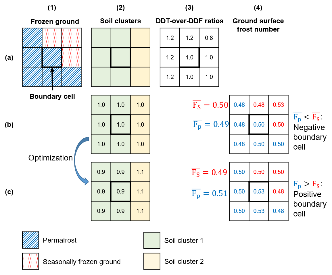
Figure C1Illustration explaining the concept of a boundary cell and the optimization process to improve boundary consistency. Column (1) shows a boundary cell in a survey-based map whose 3×3 neighboring cells contain permafrost and seasonally frozen ground. Column (2) shows two soil clusters present in the neighboring cells. The numbers in the cells indicate the values of parameter E associated with the soil clusters of the cells. Column (3) shows the DDT / DDF ratios predetermined on the grid cells. In this case, permafrost cells have DDT / DDF ratios greater than 1, indicating an unfavorable climate condition for permafrost formation. Column (4) shows the resulting ground surface frost numbers (F) for the cells. is an average of F over permafrost cells in the neighboring cells, and is an average of F over seasonal frost cells in the neighboring cells. A boundary cell is positive when is greater than . Row (b) indicates a negative boundary cell when the E values assume 1, and row (c) shows that this boundary cell becomes positive by adjusting the E values. Boundary consistency improves when negative boundary cells are converted to positive cells as much as possible (row b to row c). We added boundary consistency as part of the objective function in an effort to mitigate parametric equifinality.
The sources of data used in our mapping work are listed below. The daily MODIS LST and emissivity products (MOD11A1 and MYD11A1 Version 6) and the NDVI product (MOD13A2) are provided by NASA: https://www.earthdata.nasa.gov/. The Shuttle Radar Topography Mission 90 m digital elevation database (SRTM DEM, version 4; Reuter et al., 2007) is available at https://cgiarcsi.community/data/srtm-90m-digital-elevation-database-v4-1/. The 1 km monthly precipitation dataset for China (Peng et al., 2019) is available at https://doi.org/10.5281/zenodo.3114194. The 500 m Daily Fractional Snow Cover Dataset Over High Asia (Qiu et al., 2017) is available at https://doi.org/10.11888/GlaciolGeocryol.tpe.0000016.file. The China Data Set of Soil Properties for Land Surface Modeling (Shangguan et al., 2013) is available at http://globalchange.bnu.edu.cn/research/soil2. The China national surface weather stations (version 3.0) information is provided by the China National Meteorological Information Centre: https://data.tpdc.ac.cn/en/data/52c77e9c-df4a-4e27-8e97-d363fdfce10a/. The borehole ground temperature data provided by Zhao et al. (2021) are available at https://doi.org/10.11888/Geocry.tpdc.271107. The new permafrost distribution map on the Tibetan Plateau by Zou et al. (2017) is available at https://doi.org/10.11888/Geocry.tpdc.270468. The permafrost distribution map by Wang et al. (2019) is available at https://data.mendeley.com/datasets/ddj8ygdjbd/1. Our new 2010 permafrost distribution map and associated data are available at https://doi.org/10.6084/m9.figshare.19642362 (Cao et al., 2022). The above links have been checked and found accessible on 13 October 2022.
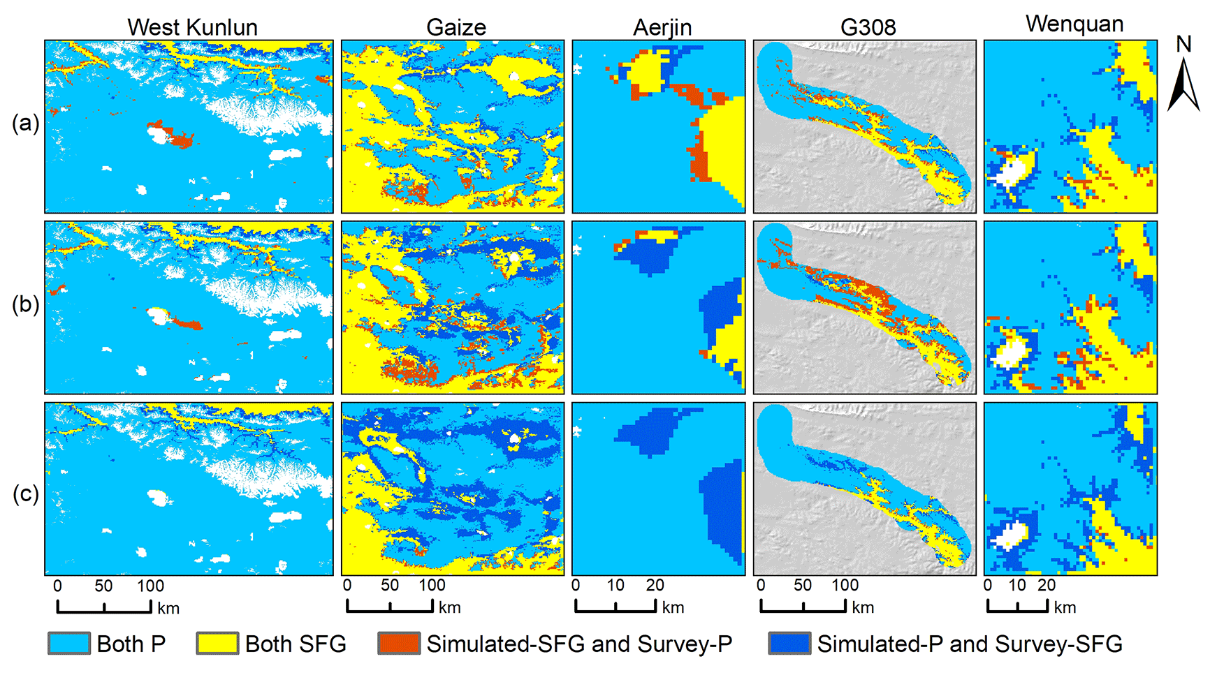
Figure E1Differences in the spatial distribution of frozen ground type in the subregions between the survey-based maps and the three simulated maps from (a) our study, (b) Zou et al. (2017), and (c) Wang et al. (2019). “Both P” represents areas identified as underlying permafrost in both survey-based and simulated maps, “Both SFG” represents areas identified as seasonally frozen ground (SFG) in both survey-based and simulated maps, “Simulated-SFG and Survey-P” represents areas identified as SFG in the simulated map but permafrost in the survey-based map, and “Simulated-P and Survey-SFG” represents areas identified as permafrost in the simulated map but SFG in the survey-based map.
Table E1Annual average soil temperatures at three depths (3, 6, and 10 m) in borehole QTB15 (33.10∘ N, 91.90∘ E) within the source area of the Yangtze River. Data were sourced from Zhao et al. (2021). The symbol “–” denotes a missing value.
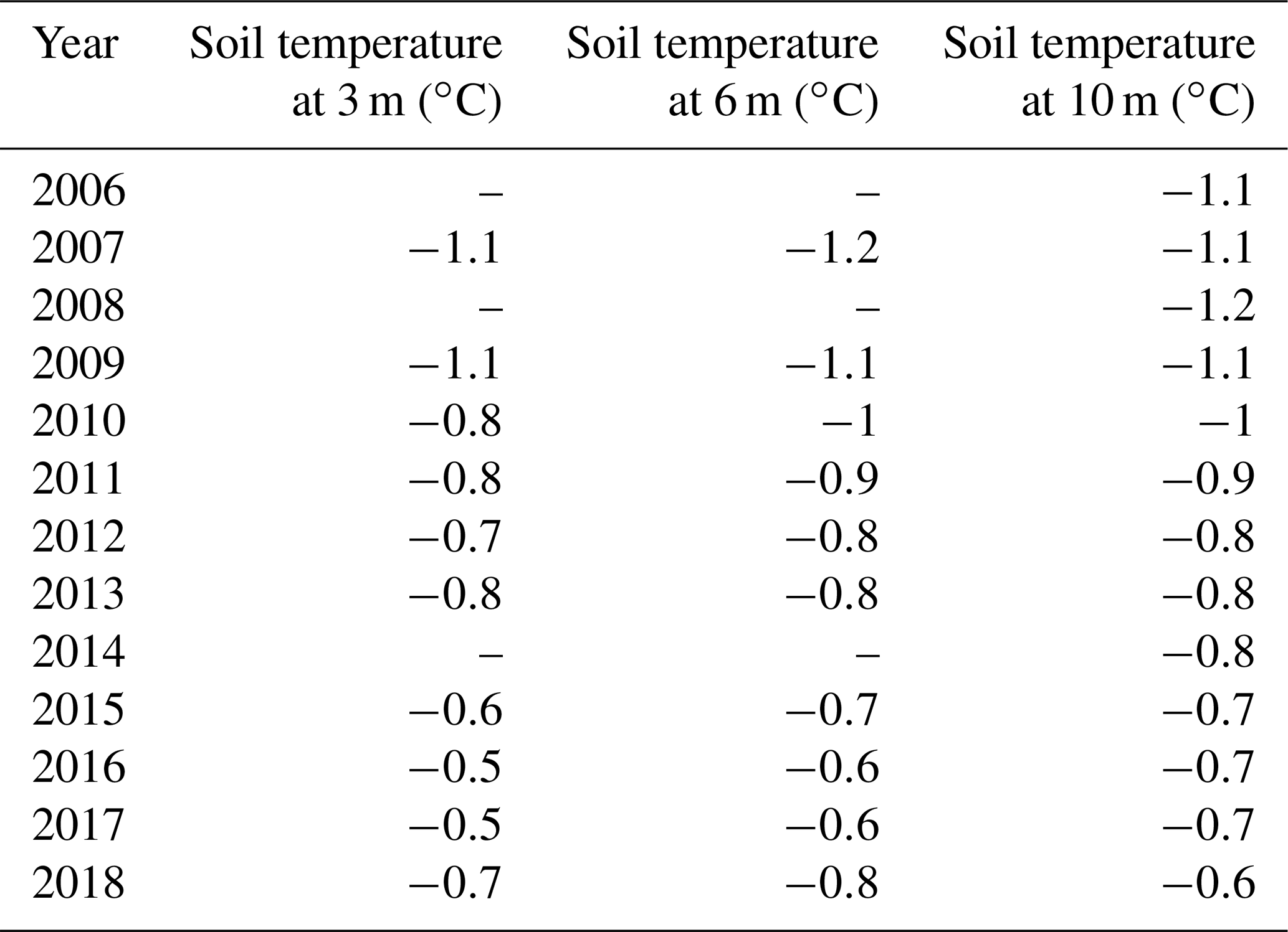
ZN: conceptualization; ZN, ZC, JH, and YC: methodology; ZC: formal analysis; ZC and ZN: writing – original draft; ZN, ZC, and YC: writing – review and editing; ZN: supervision; ZN and YZ: funding acquisition. All authors have read and agreed upon the published version of the paper.
The contact author has declared that none of the authors has any competing interests.
Publisher’s note: Copernicus Publications remains neutral with regard to jurisdictional claims in published maps and institutional affiliations.
The authors would like to thank NASA (https://search.earthdata.nasa.gov, last access: 13 October 2022), the National Tibetan Plateau Data Center (https://data.tpdc.ac.cn, last access: 13 October 2022), the National Cryosphere Desert Data Center (https://www.ncdc.ac.cn, last access: 13 October 2022), and the Science Data Bank (https://www.scidb.cn, last access: 13 October 2022) for providing the data. We also thank the scientists who participated in the Second Tibetan Plateau Scientific Expedition and Research campaign for their great work with respect to collecting valuable in situ data on the QTP. We are especially grateful to Jan Beutel and Samuel Gagnon for their valuable and profound comments on the manuscript, which greatly improved the quality of this paper.
This research has been supported by the Second Tibetan Plateau Scientific Expedition and Research (STEP) program (grant no. 2019QZKK0905-08) and the National Natural Science Foundation of China (grant nos. 41931180, 41971074, and 42171125). Zetao Cao also received support from the Postgraduate Research and Practice Innovation Program of Jiangsu Province (grant no. KYCX22_1583).
This paper was edited by Kirsten Elger and reviewed by Samuel Gagnon and Jan Beutel.
Andresen, C. G., Lawrence, D. M., Wilson, C. J., McGuire, A. D., Koven, C., Schaefer, K., Jafarov, E., Peng, S., Chen, X., Gouttevin, I., Burke, E., Chadburn, S., Ji, D., Chen, G., Hayes, D., and Zhang, W.: Soil moisture and hydrology projections of the permafrost region – a model intercomparison, The Cryosphere, 14, 445–459, https://doi.org/10.5194/tc-14-445-2020, 2020.
Burke, E. J., Zhang, Y., and Krinner, G.: Evaluating permafrost physics in the Coupled Model Intercomparison Project 6 (CMIP6) models and their sensitivity to climate change, The Cryosphere, 14, 3155–3174, https://doi.org/10.5194/tc-14-3155-2020, 2020.
Cao, B., Zhang, T., Wu, Q., Sheng, Y., Zhao, L., and Zou, D.: Brief communication: Evaluation and inter-comparisons of Qinghai–Tibet Plateau permafrost maps based on a new inventory of field evidence, The Cryosphere, 13, 511–519, https://doi.org/10.5194/tc-13-511-2019, 2019a.
Cao, B., Zhang, T., Wu, Q., Sheng, Y., Zhao, L., and Zou, D.: Permafrost zonation index map and statistics over the Qinghai-Tibet Plateau based on field evidence, Permafrost Periglac., 30, 178–194, https://doi.org/10.1002/ppp.2006, 2019b.
Cao, B., Gruber, S., Zheng, D., and Li, X.: The ERA5-Land soil temperature bias in permafrost regions, The Cryosphere, 14, 2581–2595, https://doi.org/10.5194/tc-14-2581-2020, 2020.
Cao, Z., Nan, Z., Chen, Y., and Hu, J.: A new 2010 permafrost distribution map over the Qinghai-Tibet Plateau based on subregion survey maps: a benchmark for regional permafrost modelling, figshare [data set], https://doi.org/10.6084/m9.figshare.19642362, 2022.
Cao, Z., Hu, J., and Nan, Z.: nanzt/frostnumcop: v1.0-essd (v1.0-essd), Zenodo [code], https://doi.org/10.5281/zenodo.8301453, 2023.
Chang, Y., Lyu, S., Luo, S., Li, Z., Fang, X., Chen, B., Li, R., and Chen, S.: Estimation of permafrost on the Tibetan Plateau under current and future climate conditions using the CMIP5 data, Int. J. Climatol., 38, 5659–5676, https://doi.org/10.1002/joc.5770, 2018.
Chen, J., Zhao, L., Sheng, Y., Li, J., Wu, X., Du, E., Liu, G., and Pang, Q.: Some characteristics of permafrost and its distribution in the Gaize area on the Qinghai–Tibet Plateau, China, Arct. Antarct. Alp. Res., 48, 395–409, https://doi.org/10.1657/AAAR0014-023, 2016.
Chen, Y., Nan, Z., Zhao, S., and Xu, Y.: A Bayesian Approach for Interpolating Clear-Sky MODIS Land Surface Temperatures on Areas With Extensive Missing Data, IEEE J. Sel. Top. Appl., 14, 515–528, https://doi.org/10.1109/JSTARS.2020.3038188, 2020.
Chen, Y., Nan, Z., Cao, Z., Ou, M., and Feng, K.: A stepwise framework for interpolating land surface temperature under cloudy conditions based on the solar-cloud-satellite geometry, ISPRS J. Photogramm., 197, 292–308, https://doi.org/10.1016/j.isprsjprs.2023.02.004, 2023.
Cheng, G., Li, S., Nan, Z., and Tong, B.: Map of permafrost on the Qinghai-Tibet Plateau (1:3 000 000) (1983–1996), National Tibetan Plateau Data Center [data set], https://doi.org/10.11888/Geocry.tpdc.270014, 2011.
Cheng, G., Zhao, L., Li, R., Wu, X., Sheng, Y., Hu, G., Zou, D., Jin, H., Li, X., and Wu, Q.: Characteristic, changes and impacts of permafrost on Qinghai-Tibet Plateau, Chinese Sci. Bull., 64, 2783–2795, https://doi.org/10.1360/TB-2019-0191, 2019 (in Chinese).
Cohen, J.: A coefficient of agreement for nominal scales, Educ. Psychol. Meas., 20, 37–46, https://doi.org/10.1177/001316446002000104, 1960.
Dai, L., Che, T., Xie, H., and Wu, X.: Estimation of snow depth over the Qinghai-Tibetan Plateau based on AMSR-E and MODIS data, Remote Sens., 10, 1989, https://doi.org/10.3390/rs10121989, 2018.
Debolskiy, M. V., Nicolsky, D. J., Hock, R., and Romanovsky, V. E.: Modeling Present and Future Permafrost Distribution at the Seward Peninsula, Alaska, J. Geophys. Res.-Earth, 125, e2019JF005355, https://doi.org/10.1029/2019JF005355, 2020.
Dobinski, W.: Permafrost, Earth-Sci. Rev., 108, 158–169, https://doi.org/10.1016/j.earscirev.2011.06.007, 2011.
Friedman, J. H.: Multivariate adaptive regression splines, Ann. Stat., 19, 1–67, 1991.
Gisnås, K., Etzelmüller, B., Lussana, C., Hjort, J., Sannel, A. B. K., Isaksen, K., Westermann, S., Kuhry, P., Christiansen, H. H., and Frampton, A.: Permafrost map for Norway, Sweden and Finland, Permafrost Periglac., 28, 359–378, https://doi.org/10.1002/ppp.1922, 2017.
Gruber, S.: Derivation and analysis of a high-resolution estimate of global permafrost zonation, The Cryosphere, 6, 221–233, https://doi.org/10.5194/tc-6-221-2012, 2012.
Guo, D. and Wang, H.: Simulation of permafrost and seasonally frozen ground conditions on the Tibetan Plateau, 1981–2010, J. Geophys. Res.-Atmos., 118, 5216–5230, https://doi.org/10.1002/jgrd.50457, 2013.
Guo, W., Liu, S., Xu, J., Wu, L., Shangguan, D., Yao, X., Wei, J., Bao, W., Yu, P., and Liu, Q.: The second Chinese glacier inventory: data, methods and results, J. Glaciol., 61, 357–372, https://doi.org/10.3189/2015JoG14J209, 2015.
Hachem, S., Duguay, C. R., and Allard, M.: Comparison of MODIS-derived land surface temperatures with ground surface and air temperature measurements in continuous permafrost terrain, The Cryosphere, 6, 51–69, https://doi.org/10.5194/tc-6-51-2012, 2012.
Hu, G., Zhao, L., Li, R., Wu, X., Wu, T., Zhu, X., Pang, Q., Yue Liu, G., Du, E., and Zou, D.: Simulation of land surface heat fluxes in permafrost regions on the Qinghai-Tibetan Plateau using CMIP5 models, Atmos. Res., 220, 155–168, https://doi.org/10.1016/j.atmosres.2019.01.006, 2019a.
Hu, G., Zhao, L., Wu, X., Li, R., Wu, T., Su, Y., and Hao, J.: Evaluation of reanalysis air temperature products in permafrost regions on the Qinghai-Tibetan Plateau, Theor. Appl. Climatol., 138, 1457–1470, https://doi.org/10.1007/s00704-019-02888-8, 2019b.
Hu, J., Zhao, S., Nan, Z., Wu, X., Sun, X., and Cheng, G.: An effective approach for mapping permafrost in a large area using subregion maps and satellite data, Permafrost Periglac., 31, 548–560, https://doi.org/10.1002/ppp.2068, 2020.
Huang, R., Huang, J., Zhang, C., Ma, H., Zhuo, W., Chen, Y., Zhu, D., Wu, Q., and Mansaray, L. R.: Soil temperature estimation at different depths, using remotely-sensed data, J. Integr. Agr., 19, 277–290, https://doi.org/10.1016/S2095-3119(19)62657-2, 2020.
Huang, Z.: Extensions to the k-means algorithm for clustering large data sets with categorical values, Data Min. Knowl. Disc., 2, 283–304, https://doi.org/10.1023/A:1009769707641, 1998.
Ji, H., Nan, Z., Hu, J., Zhao, Y., and Zhang, Y.: On the Spin-up Strategy for Spatial Modeling of Permafrost Dynamics: a Case Study on the Qinghai-Tibet Plateau, J. Adv. Model. Earth Sy., e2021M–e2750M, https://doi.org/10.1029/2021MS002750, 2022.
Jin, H., Luo, D., Wang, S., Lü, L., and Wu, J.: Spatiotemporal variability of permafrost degradation on the Qinghai-Tibet Plateau, Sci. Cold Arid Reg., 3, 281–305, 2011.
Koven, C. D., Riley, W. J., and Stern, A.: Analysis of permafrost thermal dynamics and response to climate change in the CMIP5 Earth System Models, J. Climate, 26, 1877–1900, https://doi.org/10.1175/JCLI-D-12-00228.1, 2013.
Kuhn, M. and Johnson, K.: Applied predictive modeling, Springer, https://doi.org/10.1007/978-1-4614-6849-3, 2013.
Li, J., Sheng, Y., Wu, J., Feng, Z., Ning, Z., Hu, X., and Zhang, X.: Landform-related permafrost characteristics in the source area of the Yellow River, eastern Qinghai-Tibet Plateau, Geomorphology, 269, 104–111, https://doi.org/10.1016/j.geomorph.2016.06.024, 2016.
Li, X., Cheng, G., Jin, H., Kang, E., Che, T., Jin, R., Wu, L., Nan, Z., Wang, J., and Shen, Y.: Cryospheric change in China, Global Planet. Change, 62, 210–218, https://doi.org/10.1016/j.gloplacha.2008.02.001, 2008.
Li, Z., Li, Z., Feng, Q., Zhang, B., Gui, J., Xue, J., and Gao, W.: Runoff dominated by supra-permafrost water in the source region of the Yangtze River using environmental isotopes, J. Hydrol., 582, 124506, https://10.1016/j.jhydrol.2019.124506, 2020.
Li, Z., Zhao, L., Liu, G., Zou, D., Wang, L., Yang, B., Du, E., Hu, G., Zhou, H., Wang, C., Xin, Z., Zhao, J., Yin, X., Chi, H., Tan, C., and Chen, W.: Analysis of soil moisture content in the active layer in the permafrost region of the Tuotuo River source in frozen season, J. Glaciolo. Geocryol., 44, 56–68, 2022 (in Chinese).
Luo, D., Jin, H., Marchenko, S. S., and Romanovsky, V. E.: Difference between near-surface air, land surface and ground surface temperatures and their influences on the frozen ground on the Qinghai-Tibet Plateau, Geoderma, 312, 74–85, https://doi.org/10.1016/j.geoderma.2017.09.037, 2018.
Marcer, M., Bodin, X., Brenning, A., Schoeneich, P., Charvet, R., and Gottardi, F.: Permafrost favorability index: spatial modeling in the French Alps using a rock glacier inventory, Front. Earth Sci., 5, 105, https://doi.org/10.3389/feart.2017.00105, 2017.
Mekonnen, Z. A., Riley, W. J., Grant, R. F., and Romanovsky, V. E.: Changes in precipitation and air temperature contribute comparably to permafrost degradation in a warmer climate, Environ. Res. Lett., 16, 24008, https://doi.org/10.1186/s40645-020-00366-8, 2021.
Mu, C., Abbott, B. W., Norris, A. J., Mu, M., Fan, C., Chen, X., Jia, L., Yang, R., Zhang, T., and Wang, K.: The status and stability of permafrost carbon on the Tibetan Plateau, Earth-Sci. Rev., 211, 103433, https://doi.org/10.1016/j.earscirev.2020.103433, 2020.
Nan, Z., Li, S., and Liu, Y.: Mean annual ground temperature distribution on the Tibetan Plateau: permafrost distribution mapping and further application, J. Glaciol. Geocryol., 24, 142–148, 2002 (in Chinese).
National Meteorological Information Centre: Daily meteorological dataset of basic meteorological elements of China National Surface Weather Station (V3.0) (1951–2010), National Tibetan Plateau Data Center [data set], https://data.tpdc.ac.cn/en/data/52c77e9c-df4a-4e27-8e97-d363fdfce10a/, 2019.
Nelson, F. E. and Outcalt, S. I.: A Computational Method for Prediction and Regionalization of Permafrost, Arct. Alp. Res., 19, 279–288, 1987.
Ni, J., Wu, T., Zhu, X., Hu, G., Zou, D., Wu, X., Li, R., Xie, C., Qiao, Y., and Pang, Q.: Simulation of the present and future projection of permafrost on the Qinghai-Tibet Plateau with statistical and machine learning models, J. Geophys. Res.-Atmos., 126, e2020J–e33402J, https://doi.org/10.1002/essoar.10503593.1, 2021.
Niu, F. and Yin, G.: Map of the frozen soil in the Tibetan Plateau (2003), National Tibetan Plateau Data Center [data set], https://doi.org/10.11888/GlaciolGeocryo.tpe.00000048.file, 2018.
Obu, J., Westermann, S., Bartsch, A., Berdnikov, N., Christiansen, H. H., Dashtseren, A., Delaloye, R., Elberling, B., Etzelmüller, B., and Kholodov, A.: Northern Hemisphere permafrost map based on TTOP modelling for 2000–2016 at 1 km2 scale, Earth-Sci. Rev., 193, 299–316, https://doi.org/10.1016/j.earscirev.2019.04.023, 2019.
Peng, S., Ding, Y., Liu, W., and Li, Z.: 1 km monthly temperature and precipitation dataset for China from 1901 to 2017, Earth Syst. Sci. Data, 11, 1931–1946, https://doi.org/10.5194/essd-11-1931-2019, 2019.
Qin, Y., Wu, T., Zhao, L., Wu, X., Li, R., Xie, C., Pang, Q., Hu, G., Qiao, Y., and Zhao, G.: Numerical modeling of the active layer thickness and permafrost thermal state across Qinghai-Tibetan Plateau, J. Geophys. Res.-Atmos., 122, 11, 604–611, 620, https://doi.org/10.1002/2017JD026858, 2017.
Qin, Y., Zhang, P., Liu, W., Guo, Z., and Xue, S.: The application of elevation corrected MERRA2 reanalysis ground surface temperature in a permafrost model on the Qinghai-Tibet Plateau, Cold Reg. Sci. Technol., 175, 103067, https://doi.org/10.1016/j.coldregions.2020.103067, 2020.
Qiu, Y., Wang, X., Han, L., Chang, L., and Shi, L.: Daily fractional snow cover dataset over High Asia, Science Data Bank, 2, 1–13, https://doi.org/10.11922/csdata.170.2017.0146, 2017 (in Chinese).
Ran, Y., Li, X., Cheng, G., Zhang, T., Wu, Q., Jin, H., and Jin, R.: Distribution of permafrost in China: an overview of existing permafrost maps, Permafrost Periglac., 23, 322–333, https://doi.org/10.1002/ppp.1756, 2012.
Reuter, H. I., Nelson, A., and Jarvis, A.: An evaluation of void-filling interpolation methods for SRTM data, Int. J. Geogr. Inf. Sci., 21, 983–1008, https://doi.org/10.1080/13658810601169899, 2007.
Shangguan, W., Dai, Y., Liu, B., Zhu, A., Duan, Q., Wu, L., Ji, D., Ye, A., Yuan, H., and Zhang, Q.: A China data set of soil properties for land surface modeling, J. Adv. Model. Earth Sy., 5, 212–224, https://doi.org/10.1002/jame.20026, 2013.
Shi, Y. and Mi, D.: Map of snow, ice, and frozen ground in China (1988), National Tibetan Plateau Data Center [data set], https://doi.org/10.3972/westdc.020.2013.db, 2013.
Shi, Y., Niu, F., Yang, C., Che, T., Lin, Z., and Luo, J.: Permafrost presence/absence mapping of the Qinghai-Tibet Plateau based on multi-source remote sensing data, Remote Sens., 10, 309, https://doi.org/10.3390/rs10020309, 2018.
Song, C., Wang, G., Mao, T., Dai, J., and Yang, D.: Linkage between permafrost distribution and river runoff changes across the Arctic and the Tibetan Plateau, Sci. China Earth Sci., 63, 292–302, https://doi.org/10.1007/s11430-018-9383-6, 2020.
Van Doninck, J., Peters, J., De Baets, B., De Clercq, E. M., Ducheyne, E., and Verhoest, N. E. C.: The potential of multitemporal Aqua and Terra MODIS apparent thermal inertia as a soil moisture indicator, Int. J. Appl. Earth Obs. Geoinf., 13, 934–941, https://doi.org/10.1016/j.jag.2011.07.003, 2011.
Wan, Z.: New refinements and validation of the MODIS Land-Surface Temperature/Emissivity products, Remote Sens. Environ., 112, 59–74, https://doi.org/10.1016/j.rse.2006.06.026, 2008.
Wang, D., Tan, D., and Liu, L.: Particle swarm optimization algorithm: an overview, Soft Comput., 22, 387–408, https://doi.org/10.1007/s00500-016-2474-6, 2018.
Wang, L., Du, Z., Wei, Z., Xu, Q., Feng, Y., Lin, P., Lin, J., Chen, S., Qiao, Y., and Shi, J.: High methane emissions from thermokarst lakes on the Tibetan Plateau are largely attributed to ebullition fluxes, Sci. Total Environ., 801, 149692, https://doi.org/10.1016/j.scitotenv.2021.149692, 2021.
Wang, S., Niu, F., Chen, J., and Dong, Y.: Permafrost research in China related to express highway construction, Permafrost Periglac., 31, 406–416, https://doi.org/10.1002/ppp.2053, 2020.
Wang, T.: 1:4 million map of the Glaciers, Frozen Ground and Deserts in China (2006), National Tibetan Plateau Data Center [data set], https://doi.org/10.3972/westdc.015.2013.db, 2013.
Wang, T., Shi, J., Ma, Y., Husi, L., Comyn Platt, E., Ji, D., Zhao, T., and Xiong, C.: Recovering land surface temperature under cloudy skies considering the solar-cloud-satellite geometry: Application to MODIS and Landsat-8 data, J. Geophys. Res.-Atmos., 124, 3401–3416, https://doi.org/10.1029/2018JD028976, 2019a.
Wang, T., Wu, T., Wang, P., Li, R., Xie, C., and Zou, D.: Spatial distribution and changes of permafrost on the Qinghai-Tibet Plateau revealed by statistical models during the period of 1980 to 2010, Sci. Total Environ., 650, 661–670, https://doi.org/10.1016/j.scitotenv.2018.08.398, 2019b.
Wang, T., Yang, D., Fang, B., Yang, W., Qin, Y., and Wang, Y.: Data-driven mapping of the spatial distribution and potential changes of frozen ground over the Tibetan Plateau, Sci. Total Environ., 649, 515–525, https://doi.org/10.1016/j.scitotenv.2018.08.369, 2019c.
Wang, W., Rinke, A., Moore, J. C., Cui, X., Ji, D., Li, Q., Zhang, N., Wang, C., Zhang, S., Lawrence, D. M., McGuire, A. D., Zhang, W., Delire, C., Koven, C., Saito, K., MacDougall, A., Burke, E., and Decharme, B.: Diagnostic and model dependent uncertainty of simulated Tibetan permafrost area, The Cryosphere, 10, 287–306, https://doi.org/10.5194/tc-10-287-2016, 2016.
Wang, Z., Wang, Q., Zhao, L., Wu, X., Yue, G., Zou, D., Nan, Z., Liu, G., Pang, Q., and Fang, H.: Mapping the vegetation distribution of the permafrost zone on the Qinghai-Tibet Plateau, J Mt. Sci., 13, 1035–1046, https://doi.org/10.1007/s11629-015-3485-y, 2016.
Westermann, S., Langer, M., and Boike, J.: Systematic bias of average winter-time land surface temperatures inferred from MODIS at a site on Svalbard, Norway, Remote Sens. Environ., 118, 162–167, https://doi.org/10.1016/j.rse.2011.10.025, 2012.
Wu, Q. and Zhang, T.: Recent permafrost warming on the Qinghai-Tibetan Plateau, J. Geophys. Res.-Atmos., 113, 1–22, https://doi.org/10.1029/2007JD009539, 2008.
Wu, X., Nan, Z., Zhao, S., Zhao, L., and Cheng, G.: Spatial modeling of permafrost distribution and properties on the Qinghai-Tibet Plateau, Permafrost Periglac., 29, 86–99, https://doi.org/10.1002/ppp.1971, 2018.
Xu, S. and Cheng, J.: A new land surface temperature fusion strategy based on cumulative distribution function matching and multiresolution Kalman filtering, Remote Sens. Environ., 254, 112256, https://doi.org/10.1016/j.rse.2020.112256, 2021.
Xu, Y., Shen, Y., and Wu, Z.: Spatial and temporal variations of land surface temperature over the Tibetan Plateau based on harmonic analysis, Mt. Res. Dev., 33, 85–94, https://doi.org/10.1659/MRD-JOURNAL-D-12-00090.1, 2013.
Yang, M., Wang, X., Pang, G., Wan, G., and Liu, Z.: The Tibetan Plateau cryosphere: Observations and model simulations for current status and recent changes, Earth-Sci. Rev., 190, 353–369, https://doi.org/10.1016/j.earscirev.2018.12.018, 2019.
Yi, S., Wang, X., Qin, Y., Xiang, B., and Ding, Y.: Responses of alpine grassland on Qinghai–Tibetan plateau to climate warming and permafrost degradation: a modeling perspective, Environ. Res. Lett., 9, 74014, https://doi.org/10.1088/1748-9326/9/7/074014, 2014.
Yin, G., Niu, F., Lin, Z., Luo, J., and Liu, M.: Data-driven spatiotemporal projections of shallow permafrost based on CMIP6 across the Qinghai-Tibet Plateau at 1 km2 scale, Adv. Clim. Chang. Res., 12, 814–827, https://doi.org/10.1016/j.accre.2021.08.009, 2021.
Yokohata, T., Saito, K., Ito, A., Ohno, H., Tanaka, K., Hajima, T., and Iwahana, G.: Future projection of greenhouse gas emissions due to permafrost degradation using a simple numerical scheme with a global land surface model, Prog. Earth Planet. Sci., 7, 1–14, https://doi.org/10.1186/s40645-020-00366-8, 2020.
Zhang, G., Yao, T., Piao, S., Bolch, T., Xie, H., Chen, D., Gao, Y., O'Reilly, C. M., Shum, C. K., and Yang, K.: Extensive and drastically different alpine lake changes on Asia's high plateaus during the past four decades, Geophys. Res. Lett., 44, 252–260, https://doi.org/10.1002/2016GL072033, 2017.
Zhang, G., Nan, Z., Wu, X., Ji, H., and Zhao, S.: The role of winter warming in permafrost change over the Qinghai-Tibet Plateau, Geophys. Res. Lett., 46, 11261–11269, https://doi.org/10.1029/2019GL084292, 2019.
Zhang, G., Nan, Z., Yin, Z., and Zhao, L.: Isolating the Contributions of Seasonal Climate Warming to Permafrost Thermal Responses Over the Qinghai-Tibet Plateau, J. Geophys. Res.-Atmos., 126, e2021JD035218, https://doi.org/10.1029/2021JD035218, 2021a.
Zhang, G., Nan, Z., Zhao, L., Liang, Y., and Cheng, G.: Qinghai-Tibet Plateau wetting reduces permafrost thermal responses to climate warming, Earth Planet. Sc. Lett., 562, 116858, https://doi.org/10.1016/j.epsl.2021.116858, 2021b.
Zhang, G., Nan, Z., Hu, N., Yin, Z., Zhao, L., Cheng, G., and Mu, C.: Qinghai-Tibet Plateau permafrost at risk in the late 21st century, Earth's Future, e2022EF002652, https://doi.org/10.1029/2022EF002652, 2022.
Zhang, L., Xia, X., Liu, S., Zhang, S., Li, S., Wang, J., Wang, G., Gao, H., Zhang, Z., and Wang, Q.: Significant methane ebullition from alpine permafrost rivers on the East Qinghai–Tibet Plateau, Nat. Geosci., 13, 349–354, https://doi.org/10.1038/s41561-020-0571-8, 2020.
Zhang, X., Zhou, J., Liang, S., and Wang, D.: A practical reanalysis data and thermal infrared remote sensing data merging (RTM) method for reconstruction of a 1-km all-weather land surface temperature, Remote Sens. Environ., 260, 112437, https://doi.org/10.1016/j.rse.2021.112437, 2021.
Zhao, H., Liu, S., Dong, S., Su, X., Wang, X., Wu, X., Wu, L., and Zhang, X.: Analysis of vegetation change associated with human disturbance using MODIS data on the rangelands of the Qinghai-Tibet Plateau, Rangeland J., 37, 77–87, https://doi.org/10.1071/RJ14061, 2015.
Zhao, L., Wu, T., Xie, C., Li, R., Wu, X., Yao, J., Yue, G., and Xiao, Y.: Support geoscience research, environmental management, and engineering construction with investigation and monitoring on permafrost in the Qinghai-Tibet Plateau, China (in Chinese), Bull. Chin. Acad. Sci., 32, 1159–1168, https://doi.org/10.16418/j.issn.1000-3045.2017.10.015, 2017.
Zhao, L., Zou, D., Hu, G., Du, E., Pang, Q., Xiao, Y., Li, R., Sheng, Y., Wu, X., and Sun, Z.: Changing climate and the permafrost environment on the Qinghai-Tibet (Xizang) plateau, Permafrost Periglac., 31, 396–405, https://doi.org/10.1002/ppp.2056, 2020.
Zhao, L., Zou, D., Hu, G., Wu, T., Du, E., Liu, G., Xiao, Y., Li, R., Pang, Q., Qiao, Y., Wu, X., Sun, Z., Xing, Z., Sheng, Y., Zhao, Y., Shi, J., Xie, C., Wang, L., Wang, C., and Cheng, G.: A synthesis dataset of permafrost thermal state for the Qinghai–Tibet (Xizang) Plateau, China, Earth Syst. Sci. Data, 13, 4207–4218, https://doi.org/10.5194/essd-13-4207-2021, 2021.
Zhao, S. P., Nan, Z. T., Huang, Y. B., and Zhao, L.: The application and evaluation of simple permafrost distribution models on the Qinghai-Tibet Plateau, Permafrost Periglac., 28, 391–404, https://doi.org/10.1002/ppp.1939, 2017.
Zou, D., Zhao, L., Wu, T., Wu, X., Pang, Q., and Wang, Z.: Modeling ground surface temperature by means of remote sensing data in high-altitude areas: test in the central Tibetan Plateau with application of moderate-resolution imaging spectroradiometer Terra/Aqua land surface temperature and ground-based infrared radiometer, J. Appl. Remote Sens., 8, 83516, https://doi.org/10.1117/1.JRS.8.083516, 2014.
Zou, D., Zhao, L., Sheng, Y., Chen, J., Hu, G., Wu, T., Wu, J., Xie, C., Wu, X., Pang, Q., Wang, W., Du, E., Li, W., Liu, G., Li, J., Qin, Y., Qiao, Y., Wang, Z., Shi, J., and Cheng, G.: A new map of permafrost distribution on the Tibetan Plateau, The Cryosphere, 11, 2527–2542, https://doi.org/10.5194/tc-11-2527-2017, 2017.
- Abstract
- Introduction
- Study area and data
- Mapping method and validation
- Results and discussion
- Data availability
- Conclusions
- Appendix A: Solar–cloud–satellite geometry (SCSG)-based interpolation approach
- Appendix B: Annual thawing index estimation
- Appendix C: An instance of boundary cell
- Appendix D: Sources of open datasets used
- Appendix E: Supplementary figures and tables
- Author contributions
- Competing interests
- Disclaimer
- Acknowledgements
- Financial support
- Review statement
- References