The Portuguese Large Wildfire Spread database (PT-FireSprd)

Wildfire behaviour depends on complex interactions between fuels, topography, and weather over a wide range of scales, being important for fire research and management applications. To allow for significant progress towards better fire management, the operational and research communities require detailed open data on observed wildfire behaviour. Here, we present the Portuguese Large Wildfire Spread database (PT-FireSprd) that includes the reconstruction of the spread of 80 large wildfires that occurred in Portugal between 2015 and 2021. It includes a detailed set of fire behaviour descriptors, such as rate of spread (ROS), fire growth rate (FGR), and fire radiative energy (FRE). The wildfires were reconstructed by converging evidence from complementary data sources, such as satellite imagery and products, airborne and ground data collected by fire personnel, and official fire data and information in external reports. We then implemented a digraph-based algorithm to estimate the fire behaviour descriptors and combined it with the Meteosat Second Generation (MSG) Spinning Enhanced Visible and Infrared Imager (SEVIRI) fire radiative power estimates. A total of 1197 ROS and FGR estimates were calculated along with 609 FRE estimates. The extreme fires of 2017 were responsible for the maximum observed values of ROS (8900 m h⁻¹) and FGR (4400 ha h⁻¹). Combining both descriptors, we describe the fire behaviour distribution using six percentile intervals that can be easily communicated to both research and management communities. Analysis of the database showed that burned extent is mostly determined by FGR rather than by ROS. Finally, we explored a practical example to show how the PT-FireSprd database can be used to study the dynamics of individual wildfires and to build robust case studies for training and capacity building.

The PT-FireSprd is the first open-access fire progression and behaviour database in Mediterranean Europe, dramatically expanding the extant information. Updating the PT-FireSprd database will require a continuous joint effort by researchers and fire personnel. PT-FireSprd data are publicly available through https://doi.org/10.5281/zenodo.7495506 (Benali et al., 2022) and have large potential to improve current knowledge on wildfire behaviour and to support better decision making.

1 Introduction

Wildfire behaviour is broadly defined as the way a free-burning fire ignites, develops, and spreads through the landscape (Albini, 1984; Rothermel, 1972). It depends on complex interactions between fuels, topography, and weather over a wide range of temporal and spatial scales (Santoni et al., 2011; Countryman, 1972). Wildfire behaviour can be described using common metrics such as the spread rate, growth rate, rate of energy release, and flame length (Albini, 1984). Fire behaviour data are important for fire research and management applications (Finney et al., 2021).

To allow for significant progress towards better fire management, the operational and research communities require detailed open data on observed wildfire behaviour (Gollner et al., 2015). In this context, systematic mapping of the fire front progression through space and time is critical to address existing needs, particularly of wildfires burning under a wide range of environmental conditions (Storey et al., 2021; Gollner et al., 2015). Compiling quality fire behaviour information is important to develop reliable and well-suited fire spread models and for a much-needed extensive evaluation of fire behaviour predictions, which is paramount in supporting the decision-making process (Alexander and Cruz, 2013; Scott and Reinhardt, 2001). This includes planning pre-suppression activities, defining resource dispatches to wildfires, and delineating safe and effective fire suppression strategies and tactics during a wildfire (Finney et al., 2021). Comprehensive fire progression and behaviour information is also useful to developing burned-area- and fire-perimeter-mapping algorithms (Valero et al., 2018), understanding fire effects (Collins et al., 2019), fire danger rating (Parisien et al., 2011), fire hazard mapping and risk analysis (Alcasena et al., 2021; Palaiologou et al., 2020), planning and implementation of preventive fuel treatments (Salis et al., 2018), and also fostering robust training of operative personnel and researchers improving their acquired knowledge from past wildfires (Alexander and Thomas, 2003). Unfortunately, reliable quality information on the progression and behaviour of wildfires, especially those burning under extreme conditions, is difficult to collect (Gollner et al., 2015).

Fire behaviour data can be collected from laboratory experiments, experimental fires, prescribed fires, or wildfires. A large number of laboratory-scale experiments have been made for the development of semi-empirical rate-of-spread (ROS) models (Rothermel, 1972; Catchpole et al., 1998). Experimental fires have been set up to collect fireline data, estimate fire behaviour descriptors, and develop empirical fire spread models (Forestry Canada Fire Danger Group, 1992; Fernandes et al., 2009; Cruz et al., 2015), requiring significant time and resources. Neither laboratory-scale nor experimental fires represent the spatial and temporal variability of the environmental conditions under which uncontrolled wildfires most often burn (e.g. Gollner et al., 2015).

Due to the unpredictability of their timing and location, conventional measurements of wildfires are difficult to perform and lead to slow accumulation of data (Alexander and Cruz, 2013). Generally, they are of poor quality or are incomplete (Duff et al., 2013), although outstanding reconstruction examples exist (e.g. Wade and Ward, 1973; Alexander and Lanoville, 1987; Cheney, 2010). Dedicated efforts do exist (Vaillant et al., 2014), but wildfire behaviour estimates often result from opportunistic observations (e.g. Santoni et al., 2011) or post-fire interviews (e.g. Butler and Reynolds, 1997). Some authors have made relevant efforts in compiling a large amount of field observations on wildfire behaviour (Alexander and Cruz, 2006; Cheney et al., 2012), some combined with experimental fire data (Cruz and Alexander, 2013, 2019; Anderson et al., 2015; Cruz et al., 2018, 2021, 2022; Khanmohammadi et al., 2022). An additional limitation lies in the fact that some of the existing fire behaviour datasets are not freely available to the operational and research communities (Gollner et al., 2015).

Remote sensing technology, either through airborne or satellite platforms, can provide relevant data to document wildfire propagation. Manned or unmanned airborne visible and infrared (IR) images have been used to map fire progression (Schag et al., 2021; Storey et al., 2020, 2021; Coen and Riggan, 2014; Sharples et al., 2012). Satellite data provide easy-to-use, autonomous, synoptic observations of fire activity worldwide. Recent advances in satellite technology have made available a panoply of open-access imagery and products with capabilities to monitor wildfires over the entire globe. Their characteristics vary in resolution, ranging from high (10–30 m) to low (4–5 km), and in frequency of overpass, ranging from 5–15 d to every 15 min. To monitor wildfire progression, satellites provide imagery and products that identify where a fire is actively burning at the time of overpass (thermal anomalies or active-fire products). Several authors have used satellite data to map daily fire progression at the country level (Parks, 2014; Veraverbeke et al., 2014; Briones-Herrera et al., 2020; Sá et al., 2017) and at the global scale (Artés et al., 2019; Oom et al., 2016). Some have estimated fire behaviour metrics, such as ROS (Humber et al., 2022; Frantz et al., 2016; Andela et al., 2019). Recently, Chen et al. (2022) improved this research line by using Visible Infrared Imaging Radiometer Suite (VIIRS) data to automatically reconstruct sub-daily fire progression at a higher resolution. Other authors exploited the capabilities of geostationary satellites to monitor wildfires and estimate fire behaviour descriptors (Sifakis et al., 2011; Storey et al., 2021).

The different data sources used to characterize wildfire progression and behaviour have inherent limitations and potentialities. Ground-collected data can be characterized by large uncertainties, particularly when taken by fire personnel whose focus is on suppression and not on data collection (Alexander and Thomas, 2003). In addition, ground-collected data have poor synoptic capability and provide a limited representation of fire behaviour variability. For example, distribution of ROS values for single fire runs are seldom available (Cruz, 2010). Airborne data can provide wider coverage of the fire progression, although they have limited temporal acquisition windows (e.g. USFS National Infrared Operations – NIROPS – provides data once per night) and in some cases require manual digitization of fire perimeters (Stow et al., 2014; Veraverbeke et al., 2014; Storey et al., 2021).

The trade off between the spatial and temporal resolution of satellite data, as well as the presence of clouds and thick smoke, can significantly limit their fire-monitoring capability. In addition, the correct location of a wildfire cannot be determined inside a burning pixel whose size varies with viewing geometry and sensor properties (Wolfe et al., 1998). Daily or sub-daily satellite-derived fire progressions can also fail to reflect the influence of extreme conditions on fire behaviour due to the effect of averaging over relatively long periods (Collins et al., 2019).

Considering that all data sources have limitations and provide information for very limited periods, combining different sources is key to capturing the spread and behaviour variability of wildfires. The example provided in Fig. 1 highlights the potential of combining different data sources to overcome inherent acquisition gaps, particularly in the afternoon, when both field and airborne data overcome the satellite gap, and during dawn, when ground-collected and satellite data complement each other. Note that observation frequencies of ground and airborne data strongly depend on daily fire activity patterns.

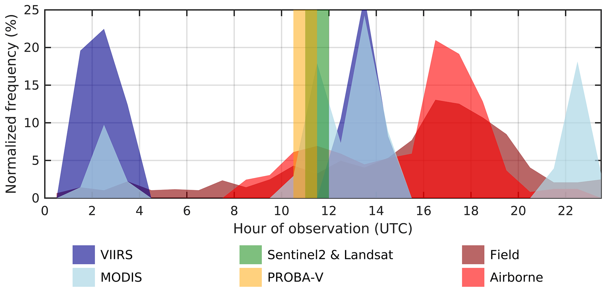
Figure 1 Hourly frequency of observations in active wildfire acquisitions for satellite, field, and airborne data. The data used refer to the year 2019 as an example. The frequency is normalized by dividing the number of observations by the total of each data source. Sentinel-2, Landsat, and PROBA-V refer to the temporal windows and not the frequency since all of the data are acquired in a very short window. The time windows of Sentinel-3 are similar to those of MODIS. MSG-SEVIRI data are not represented since it has a 15 min frequency. Acronyms are described in the Data and methods section.

Systematic multi-source acquisition of wildfire data was recently done by Kilinc et al. (2012) and Storey et al. (2020, 2021) for Australia, by Crowley et al. (2019) for Canada (only satellite data), and by Fernandes et al. (2020) at the global scale. The pursuit of this goal requires a monitoring framework and a concerted joint effort between research and operational communities (Stocks et al., 2004; McCaw et al., 2012; Storey et al., 2020, 2021). Additional data on constantly evolving wildfires, accompanied by robust replicable methods, are needed, namely in southern Europe where there is a substantial data gap (Fernandes et al., 2018).

Here, we present the Portuguese Large Wildfire Spread database (PT-FireSprd), which combines data from multiple sources and uses a convergence-of-evidence approach to characterize in detail the progression and behaviour of large wildfires in Portugal. Fire behaviour is described sensu stricto; thus, analysis of its drivers, namely weather and fuel, and its effects is beyond the scope of the current work. The work results from a joint co-creation effort between researchers and fire personnel, integrating data collected from airborne and ground operational resources.

2 Data and methods

2.1 Overview

We first collected data for all the large wildfires (> 100 ha) that occurred in mainland Portugal between 2015 and 2021. Out of 14 973 wildfires that occurred during this period, 793 (about 5 %) had an extent larger than 100 ha. These were responsible for almost 1 million ha burned, of which half occurred in the extreme-fire season of 2017. About 90 % of the total burned area resulted from the 760 largest wildfires.

Multi-source input data (L0, Sect. 2.2) were collected, and only wildfires with good-quality data that were representative of the spread were kept. Fire progressions were reconstructed from the input data, and fire behaviour metrics were estimated. The PT-FireSprd database was then organized into three levels:

• L1 comprises wildfire progression (Sect. 2.3), representing the spatial and temporal evolution of the wildfire spread (i.e. where and when).

• L2 comprises the wildfire behaviour (Sect. 2.4), including quantitative behaviour descriptors of how a wildfire burned, such as the rate of spread (ROS), fire growth rate (FGR), fire radiative energy (FRE), and FRE flux.

• L3 comprises simplified wildfire behaviour (Sect. 2.5), averaging behaviour descriptors over longer periods that represent relatively homogenous fire runs.

The data from the different levels were composed by a large set of maps that can be useful for several applications and target users. For example, L1 data can be used by fire analysts or researchers to evaluate suppression strategies and understand the fire spread drivers or to evaluate burned-area- and/or fire-perimeter-mapping algorithms. L2 data are useful, for example, for calibrating existing or building better fire spread models, while potential applications of L3 are improving fire danger rating, fire hazard mapping, and risk analysis. The overall flow of the data and methods is described in Fig. 2.

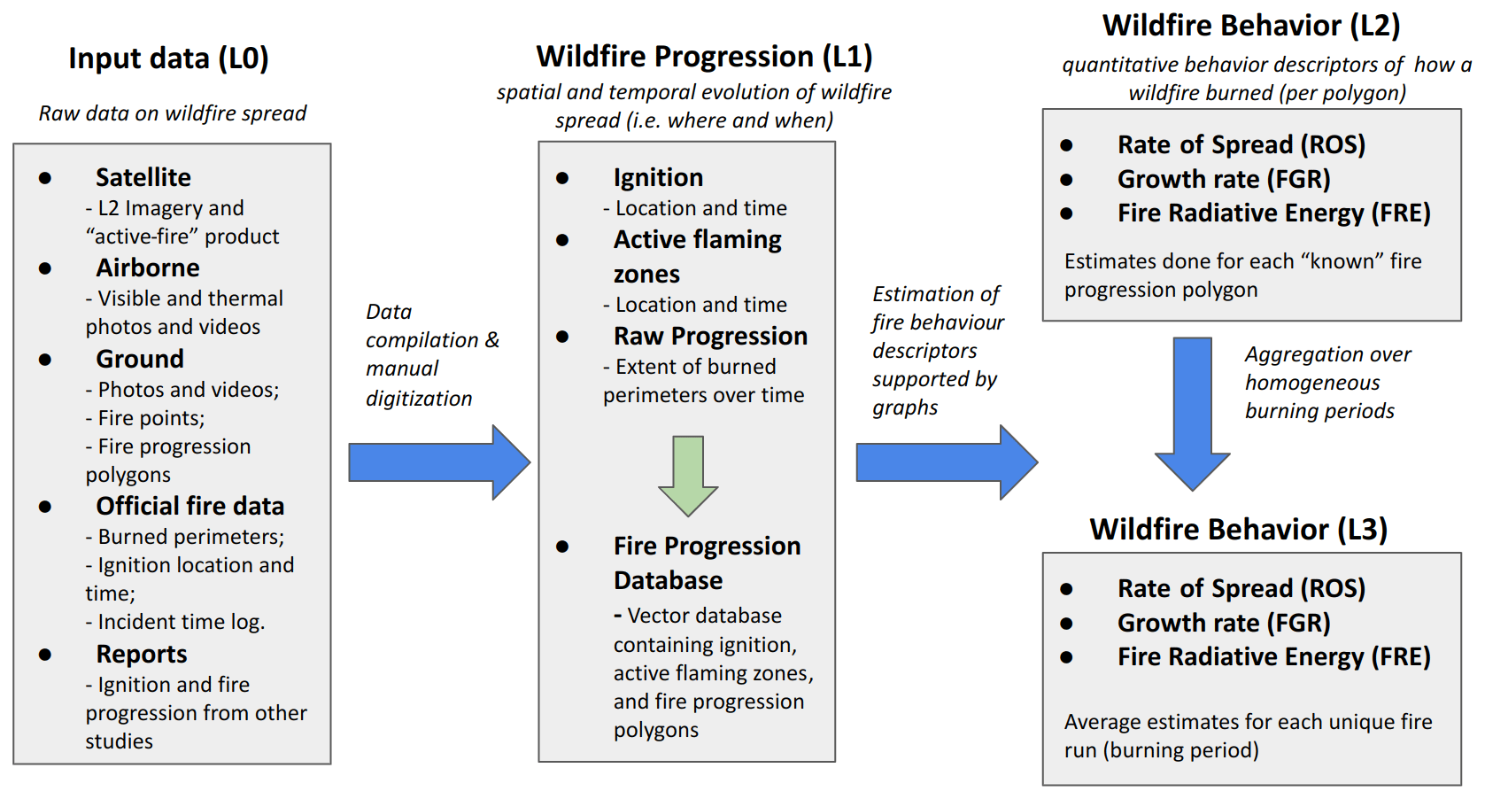
Figure 2 Flowchart that represents an overview of the data and methods used in the development of the PT-FireSprd database.

2.2 Input data (L0)

To reconstruct the wildfire progressions, we used data acquired by satellites, from airborne sources, and in the field by fire personnel. Most of these data are currently integrated in a near-real-time operational WEB-GIS fire-monitoring platform (in Portuguese: “FEB Monitorização”, hereafter FEBMON) developed in 2018 by the Civil Protection Special Force (FEPC) and the Portuguese National Authority for Emergency and Civil Protection (ANEPC). The data were complemented with official fire data and information from external reports. Table A1 in the Appendix summarizes the different data sources used and their main characteristics.

2.2.1 Satellite data

The Sentinel-2 Multispectral Instrument (MSI) and the Landsat 8/9 Operational Land Imager (OLI) provide images, on average, every 5 d and every 16 d respectively, with a spatial resolution ranging between 10 and 60 m. PROBA-V (Project for On-Board Autonomy – Vegetation) has a low number of spectral bands (four) and provides daily images at a 300 m spatial resolution and every 5 d with a 100 m spatial resolution. The VIIRS instrument aboard the NPP (National Polar-orbiting Partnership) and NOAA-20 (National Oceanic and Atmospheric Administration - 20) satellites collects data, on average, twice per day with a resolution of 375 and 750 m. The Moderate-Resolution Imaging Spectroradiometer (MODIS) is an instrument on board the TERRA and AQUA satellites with spatial resolutions ranging from 250 to 1000 m, providing, on average, four daily revisits when combined. Sentinel-3 satellites have onboard the Sea and Land Surface Temperature Radiometer (SLSTR) and the Ocean and Land Color Instrument (OLCI), with spatial resolutions ranging between 500 and 1000 m for the former and of 300 m for the latter. Data are acquired, on average, twice per day, but the OLCI does not retrieve nighttime data.

We used atmospherically corrected (L2) satellite imagery to create false-colour composites that could highlight burned areas (low near-infrared (NIR), high shortwave-infrared (SWIR) reflectance), active flaming areas (high SWIR and/or thermal-infrared (TIR) reflectance) and unburned vegetation (high NIR reflectance). Typical false-colour composites use bands 12–8A–4 of Sentinel-2, bands 7–2–1 for MODIS, and bands 1–2–4 for PROBA-V. Most imagery was downloaded from the Sentinel EO Browser (https://apps.sentinel-hub.com/eo-browser/, last access: December 2022), Worldview (https://worldview.earthdata.nasa.gov/, last access: December 2022) and VITO-EODATA (https://www.vito-eodata.be/PDF/, last access: December 2022), which allow easy and fast access to historical L2 data.

To complement the satellite imagery, we used the thermal anomaly products of VIIRS (VNP14IMGML-C1; Schroeder et al., 2014) and MODIS (MCD14ML-C6; Giglio et al., 2003, 2016), with 375 m and 1 km resolution at nadir respectively. Data are available at https://fuoco.geog.umd.edu (last access: December 2022) and FIRMS (https://firms.modaps.eosdis.nasa.gov/, last access: December 2022). These products allow an estimation of the approximate location and timing of an active wildfire and provide an estimate of the fire radiative power (FRP), a proxy of the radiant energy released per time unit, and a proxy for fuel consumption and fireline intensity. In addition, coarse-resolution data (∼ 4 km) from the Spinning Enhanced Visible and Infrared Imager (SEVIRI) sensor on board the Meteosat Second Generation (MSG) geostationary satellite were used to characterize the temporal evolution of fire activity using FRP estimates every 15 min (Wooster et al., 2015). Data are available at https://landsaf.ipma.pt/en/products/fire-products/frpgrid/ (last access: December 2022). The FRP detections associated with each wildfire were identified using a spatio-temporal nearest-distance algorithm. An empirical threshold derived from the analysis of a selected number of wildfires was used to account for the satellite pixel geolocation and temporal reporting uncertainties. The fire radiative energy (FRE) was estimated based on the FRP detections, assuming a constant rate of energy release every 15 min, and was then aggregated into 30 min bins (Eq. 1):

$$\begin{array}{}\text{(1)}& {\mathrm{FRE}}_i=\mathrm{0.0009}\times \left({\sum }_{k=\mathrm{1}}^{\mathrm{2}}{\mathrm{FRP}}_k\right),\end{array}$$

where index i indicates a 30 min bin, index k indicates the 15 min FRP value in megawatts (MW), and the 0.0009 factor converts the sum into terajoules (TJ) (Pinto et al., 2018).

2.2.2 Airborne data

Some aeroplanes and helicopters that operate during wildfires collect photos and videos. Data are collected during the initial attack (i.e. up to 90 min after the alert) by the heli-brigades of the National Guard (GNR) using their mobile phones and, occasionally, during extended attack. Aeroplanes, operated by FEPC/ANEPC since 2018, carry visible and thermal cameras that collect photos and videos during extended attack, covering the entire active-fire perimeter. In addition, helicopters that coordinate aerial suppression also collect photos and videos. Both data sources collect data only during the daytime (with a few exceptions) at relatively low altitudes.

Airborne data are systematically uploaded in real time in FEBMON, providing high-quality information regarding the probable location of the fire start, active flaming zones, and especially wildfire progression. It is worth mentioning that airborne footage is not synoptic as different parts of the wildfire (e.g. left flank vs. right flank) are captured at different moments, which, depending on the fire extent and operational priorities, can result in large acquisition time lags.

2.2.3 Ground data

The FEBMON system is linked to portable devices that allow for the collection of georeferenced ground data during wildfires by fire personnel from several entities. Ground-collected data consist of three main types: (i) photos and videos; (ii) points that identify active flaming combustion, inactive flaming or smouldering, or locations requiring mop up; and (iii) polygons that delineate an area burned until the time of acquisition (i.e. fire progression).

Besides the data automatically linked to FEBMON, valuable ad hoc information was used to reconstruct wildfire spread, such as additional photos ad/or videos and post-fire interviews. In sum, data collected by fire personnel in the field provided valuable spatiotemporal information regarding wildfire spread, ignition, and/or re-activation.

2.2.4 Official fire data

The burned-area perimeters for the entire country were provided by ICNF (Instituto da Conservação da Natureza e das Florestas), derived from a combination of fieldwork and satellite data (https://geocatalogo.icnf.pt/, last access: December 2022). Errors in the burned-area perimeters were corrected manually using Sentinel-2 or Landsat 8/9 post-fire false-colour composites (see Sect. 2.2.1). For a very limited number of very large multi-day wildfires, we used burned areas (resolution of 1.5 m) provided by the Copernicus Emergency Management Service (https://emergency.copernicus.eu/mapping/, last access: December 2022).

Regarding ignition data, we used the official wildfire start location, typically derived from post-fire investigation (ICNF, https://fogos.icnf.pt/sgif2010/, last access: December 2022), and the ignition location provided by first responders and time of alert (ANEPC). Ignition data have several known issues (Pereira et al., 2011), the most relevant of which, for the purposes of the present study, is the accuracy of its exact location.

Finally, we analysed the official wildfire time logs from ANEPC, which seldom contain useful contextual information on wildfire location at a given date or hour.

2.2.5 Reports of 2017 large wildfires

We used ignition and fire progression data published in reports of the very large wildfires of June 2017, including the Pedrogão Grande wildfire, and of October 2017 (Guerreiro et al., 2017, 2018; Viegas et al., 2019). Regarding Guerreiro et al. (2017, 2018), the primary data sources used to reconstruct the fire progression were satellite imagery, thermal-anomaly data, and burned-area perimeters provided by the Copernicus Emergency Management Service. Reports from ANEPC and the Portuguese Institute for the Sea and the Atmosphere (IPMA), GNR, and the Association for the Development and Industrial Aerodynamics (ADAI) were also used to identify fire arrival times and active fire lines. Additionally, other data sources allowed for the reconstruction of wildfire spread, such as the official wildfire time log (see Sect. 2.2.4), interviews (fire personnel involved in suppression and local residents), fieldwork to identify the forward fire spread direction, and other relevant data such as photos and videos. The fire spread isochrones were determined through spatial interpolation methods (spline and inverse distance weighting) on high-density point clouds and through experts' knowledge.

Viegas et al. (2019) reconstructed the extreme wildfires of October 2017 based on fieldwork, interviews, photos and videos, and information contained in the official wildfire time log. Since the fire progression data were not provided by the authors, here we used only very limited information regarding ignition location and time and general fire spread patterns, mostly to complement data provided by Guerreiro et al. (2017, 2018).

Persistent cloud cover hindered the June and October 2017 wildfire progression mapping with satellite data. Nonetheless, given the relevance of these wildfires, we decided to include these fire progressions in our database because they represent some of the largest and most extreme wildfires that ever occurred in mainland Portugal.

2.3 Wildfire progression (L1)

Wildfire progression characterizes the spatial and temporal evolution of the area burned in a specific fire event. To reconstruct wildfire progression, we combined the maximum available data from the different sources mentioned above with the aim of obtaining convergence of evidence. This allowed us to reduce the limitations and uncertainties of each individual data source and to build higher confidence in the derived wildfire progression.

L1 data also contain information regarding the ignition time and location, as well as flaming zones that correspond to active areas during the wildfire spread. These include spot fires and reactivation or rekindling areas. Combining all the available data, we manually delimited the extent and time of the ignition, fire progression, and active flaming zones of each wildfire. The reconstruction was made chronologically, i.e. starting from ignition and ending with the progression prior to wildfire containment. Sentinel-2 and Landsat 8/9 pre-fire images were used to identify areas burned shortly before the wildfire, and post-fire images were used to correct each progression polygon. As an example, Fig. 3 shows how different data sources were combined to derive the spread of the Castro Marim (2021) wildfire. All wildfire progressions (L1) were defined as polygons, each with a set of different attributes (explained below).

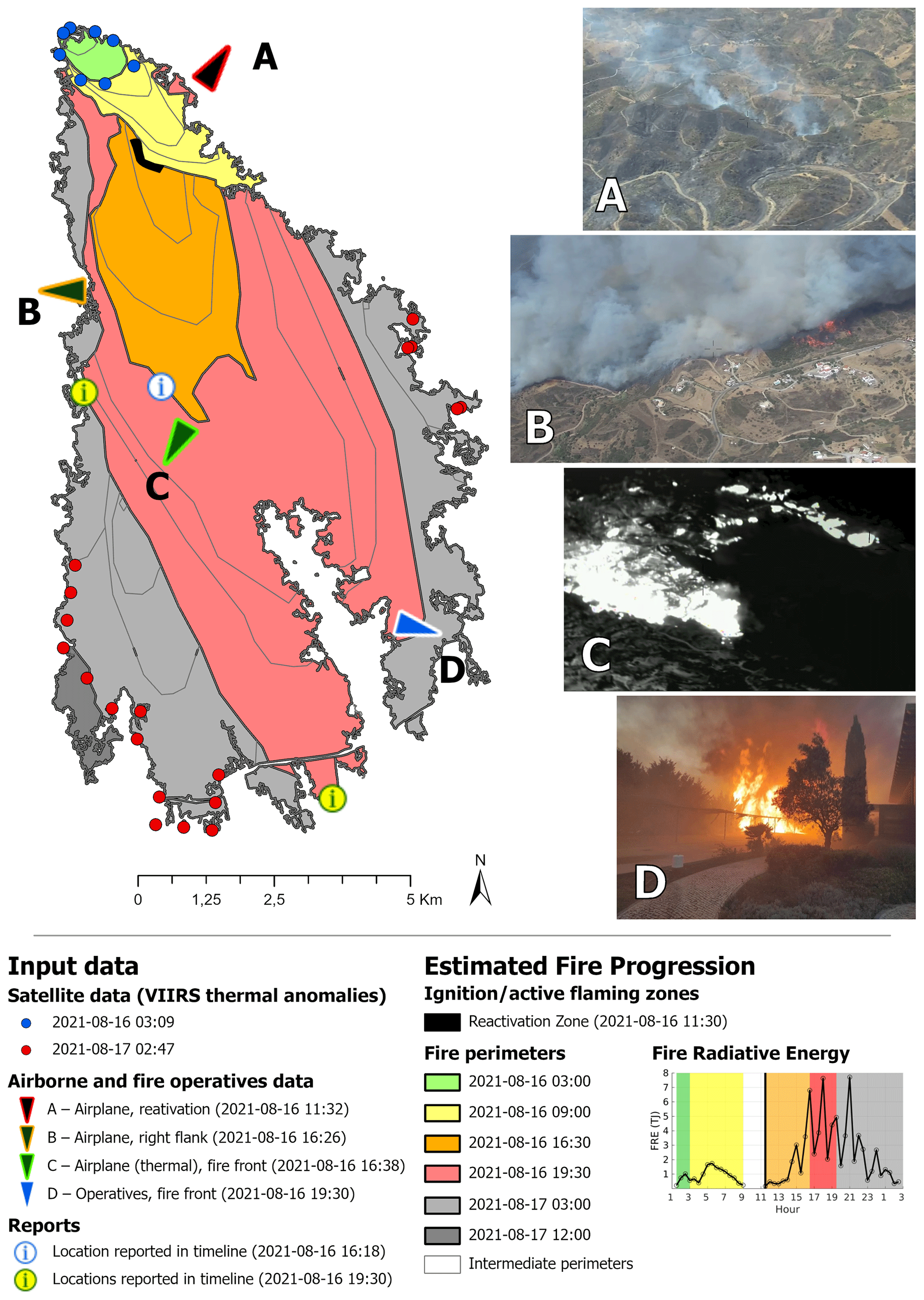
Figure 3 Example of multi-source data integration to derive fire perimeters and reconstruct the progression of the Castro Marim (2021) wildfire. The lines represent different progression polygons. Photos A, B, C, and D were kindly provided by ANEPC/FEPC.

Ignition location was defined as an area (vector polygon) instead of a point to account for spatial uncertainties and to have a common data typology for the entire database. To define ignition location, we used mostly official data, ignition location provided by first responders, and initial-attack airborne photos. This was complemented with expert knowledge and information from fire personnel. For a small set of wildfires (mostly with nighttime ignitions), we also used satellite active-fire data to map the approximate ignition location. All ignitions were compared with later fire spread patterns and with the final burned area to reduce errors and guarantee consistency (e.g. ignition was contained in the final burned area). The official time of alert was compared with 15 min MSG-SEVIRI FRP data to confirm the alert time or, in a very few cases, to anticipate the ignition time if energy was released before. MSG-SEVIRI FRP data were also useful for the identification (or confirmation) of the timing of reactivation(s). An example is shown in Fig. 3, where the significant release of energy around 11:30 LT (local time), combined with ground data allowed for the identification of the location and time of the reactivation zone.

Active flaming zones were mostly derived from ground and airborne data and/or high-spatial-resolution satellite imagery. Alternatively, they were defined based on visual interpretation of multiple moderate-resolution satellite imagery and were often combined with active-fire data (mostly VIIRS due to its higher spatial resolution). Inconclusive visual interpretations were discarded, as well as active zones that did not lead to any relevant subsequent fire spread. The ignition zone and all active flaming zones were always contained within the subsequent fire spread polygon.

Wildfire progression was represented by a series of consecutive polygons delineating the temporal evolution of the area burned by the wildfire. The number of polygons depended on fire size and data availability. The progression polygons were built using as many data sources as possible, complementing each other in both space and time (see Fig. 1). The varieties of input data used have different associated uncertainties. When delineating the progression polygons, priority was given to input data with higher spatial resolution, free from smoke and cloud contamination, and with the most complete view of the entire active part of the wildfire. Typically, the first-priority-level data (i.e. highest confidence) were Sentinel-2 and Landsat 8/9 images and AVRAC aeroplane photos and videos. The second priority level was composed of ground data, VIIRS active fires, PROBA-V and Sentinel-3 images (both at 300 m resolution), and helicopter photos and videos. The third priority level was composed of images and active-fire data from moderate-resolution satellites (MODIS and Sentinel-3). The fourth and last priority level (i.e. lowest confidence) was composed of FRP data from MSG-SEVIRI and the official wildfire time logs. The data from the large 2017 wildfires reports were handled separately. The progression polygons from Guerreiro et al. (2017, 2018) were deemed to be high-confidence data and were complemented with data and information from Viegas et al. (2019) and, at times, with satellite data.

A common challenge found in the delineation of the wildfire progression was the uncertainties associated with the correct time an entire progression polygon burned. These uncertainties were present in almost all data sources. For example, a polygon derived by fire operatives on the ground could have stopped burning minutes or hours before data collection. Additionally, satellite active-fire data can depict areas that are hot minutes or hours after the fire front stopped progressing. The strategy to minimize such uncertainties was to use data from multiple sources, seeking convergence of evidence. As an example, a common feature found in the data was substantial fire spread during daytime followed by very limited nighttime progression. In these cases, first, the nighttime fire progression was delineated using active-fire data (mostly VIIRS) and complemented with ground data, when available. Second, satellite and/or airborne imagery acquired the following morning were used to perform any necessary adjustments in the nighttime spread polygon(s). FRE estimates of MSG-SEVIRI were also used to identify if any substantial fire activity occurred between VIIRS and MODIS nighttime overpass and daytime imagery (satellite and/or airborne). We assumed that fire activity decreased significantly when the wildfire released less than 0.5 TJ per 30 min period and anticipated the date and/or hour of the fire spread polygon accordingly. In smaller wildfires (< 500 ha), this threshold was set to 0.1 TJ. Such thresholds were defined empirically (see Discussion section). The entire procedure reduced the uncertainties associated with the definition of the end date and/or time of the progression polygons. It should be noted that the fire behaviour within the time span of each progression polygon was unknown; therefore, it was assumed to be free burning at a constant rate (Storey et al., 2021). When data were insufficient to determine when a given area burned, the spread polygon was flagged as uncertain.

Ignitions and active flaming zones were linked to the resultant spread polygon(s) by assigning a numeric label to a field called zp_link, providing an explicit connection between both and allowing us to track the source of a given progression polygon. When information was insufficient, for example, when the start of the progression polygon was unknown, zp_link was set to 0. After all ignition(s), fire progressions, and active flaming zones were defined, each wildfire was divided into burning periods. We assumed that each burning period contained relatively homogeneous fire runs, such that

• i.

  they were ignited by the same set of ignitions or active flaming zones,

• ii.

  they did not exhibit large fire spread direction shifts (less than 45^∘ of variation),

• iii.

  they were not impeded by barriers (e.g. previously burned area), and

• iv.

  they did not exhibit significant changes in fire behaviour (e.g. large ROS variation).

Regarding the latter criterion, for example, daytime and nighttime runs were usually separated into different burning periods, even if criteria (i) to (iii) were fulfilled. By definition, a new active flaming zone always marked the beginning of a new burning period; however, not all burning periods started with an ignition or active flaming zone since this depended on data availability.

When direct evidence of fire spotting was available (i.e. exact location and timing of the spot fire(s), typically from ground and/or airborne data), if the fire front(s) rapidly (under 1 h) coalesced with the original fire front, fire progression was merged into a single polygon. In the remaining cases, typically associated with medium-distance spotting and/or slow-burning fire fronts, the spotting location was defined as a new active-flaming-zone setting, defining a new burning period. When the exact location and timing of the spot fire was not available, evidence of spotting consisted of observations of non-contiguous burned areas that resulted from the same wildfire. These were typically separated by rivers, lakes, and settlements. In these cases, due to lack of data, the polygons separated from the major fire run were defined with zp_link = 0 if the distance was larger than 200 m. No fire behaviour descriptors were calculated for these polygons.

The definition of the burning period was always dependent on data availability and, in some cases, was subjective. For the progressions derived using only satellite data, the length of the burning period was mostly determined by the timing of the satellite overpass(es) and the FRE's temporal evolution. For the progressions derived from more detailed data, the above-mentioned criteria were easier to fulfil. In a few cases, uncertainties in fire progressions led to slightly overlapping periods. An example is shown in the Results section, and implications are addressed in the Discussion section.

After collecting input data for a large number of wildfires, only those with at least one valid progression, ignition, and active flaming zone were kept. We eliminated all suspicious cases where uncertainties were large, for example, due to the presence of persistent smoke or clouds in the satellite or airborne images or the absence of valid ground data. The L1 wildfire progression database was defined by a set of polygons with attribute fields (details in Sect. 5). The date and hour of each ignition, fire spread, and active flaming zone (if applicable) were approximated to the nearest 30 min period. Fire progression data from external reports were adapted to the rationale of the fire database described above.

2.4 Wildfire behaviour (L2)

Fire behaviour descriptors were estimated using spatial graphs. A graph is a mathematical structure composed of nodes (N) and edges (E), which connect the nodes (Dale and Fortin, 2010). Based on the fire spread polygons (L1) (Fig. 4a), we built a spatial directed graph (or digraph) where each node refers to a spread polygon, and each edge connects two spread polygons (i.e nodes) with a valid link (i.e. zp_link > 0). These two nodes burned at different times, one earlier (t_i) and the other later (t_j). The value of each edge was defined as the time elapsed between two nodes (Δt_ij) (Fig. 4b). A node can have an inward edge (where fire is transmitted from) and an outward edge (where fire is transmitted to).

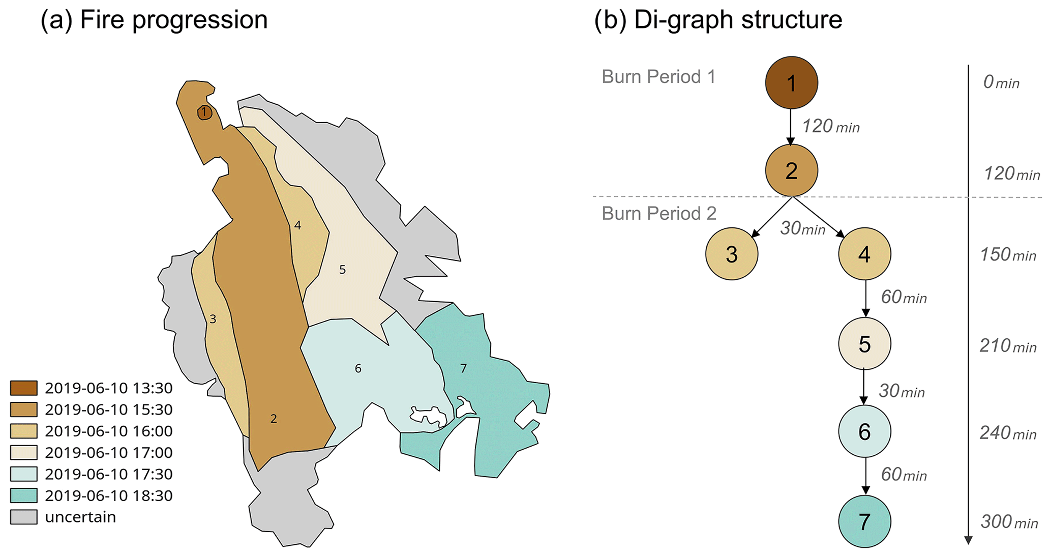
Figure 4 Example of how the estimated fire progression of the Ourique 2019 wildfire (a) was used to build the digraph (b). Each node corresponds to a fire progression polygon, identified in (a), and the edges correspond to the time elapsed (in minutes) between each node.

First, the nodes were connected only if the associated fire progression polygons were contiguous, had the same zp_link value, and burned at different timings. Second, only the edges corresponding to the shortest elapsed time between two nodes were kept. The digraph allowed us to formally structure the connections between fire spread polygons, enabling the calculation of fire behaviour descriptors.

To allow for a better understanding of the methods used, a brief explanation based on the Ourique (2019) wildfire is provided. In Fig. 4, the number of the polygons on the left matches the number of nodes on the right. After its start (1), the wildfire spread fast to the south and burned the area delimited by polygon 2 in about 120 min. Fire behaviour changed after the head run, and the left flank became the head and subsequently made a run to the southeast, burning the area represented by polygons 4, 5, 6, and 7, in about 180 min. This fire behaviour change observed at t=120 min determined the definition of two burning periods: one corresponding to the initial head run, the other corresponding to head run from the left flank. The digraph was built with seven nodes and six edges, with values ranging between 30 and 120 min.

Based on the fire progression (L1) and the corresponding digraph, we calculated the following set of fire behaviour descriptors (L2): forward ROS (m h⁻¹), direction of forward spread (^∘ from north), FGR (ha h⁻¹), and FRE (TJ). The polygons referring to areas burned shortly before the fire analysed were removed from L2.

ROS was calculated for each node (N_j), with a valid inward edge (E_ij) connecting it to a prior node (N_i). By definition, the forward ROS refers to the head of the fire and was calculated considering the longest distance line connecting two consecutive fire progression polygons (i.e. nodes) representing the fastest spread (Storey et al., 2021). The ground distance (D_ij) between each pair of polygons was calculated as follows:

• All ground distances between the polygon vertices of N_i and N_j were calculated using the European Digital Elevation Model (EU-DEM v1.1, https://land.copernicus.eu/imagery-in-situ/eu-dem/eu-dem-v1.1, last access: December 2022) resampled to 50 m spatial resolution.

• For each vertex of the N_j polygon, only the shortest distance was kept, and the corresponding pair of vertices, from N_i and N_j, were stored.

• D_ij was defined as the maximum of all the shortest distances between vertices.

The ROS was calculated by dividing the distance (D_ij) by the time elapsed between the pair of polygons (Δt_ij) and was expressed in metres per hour (m h⁻¹). We divided the ROS calculation into two distinct measures:

• partial ROS (hereafter ROSp) calculated between two consecutive polygons

• mean ROS (hereafter ROSi) calculated between the ignition (or active flaming front) and a given spread polygon.

The spread direction was calculated using trigonometric rules considering the two above-mentioned vertices between two polygons. The spread direction was calculated for both ROSp and ROSi, where the difference lies only in the origin polygon. FGR was calculated by dividing the burned area by each polygon or node (A_j) by the time elapsed between polygons (Δt_ij) and was expressed in hectares per hour (ha h⁻¹). An example of the calculation of these fire behaviour descriptors is shown in Fig. 5.

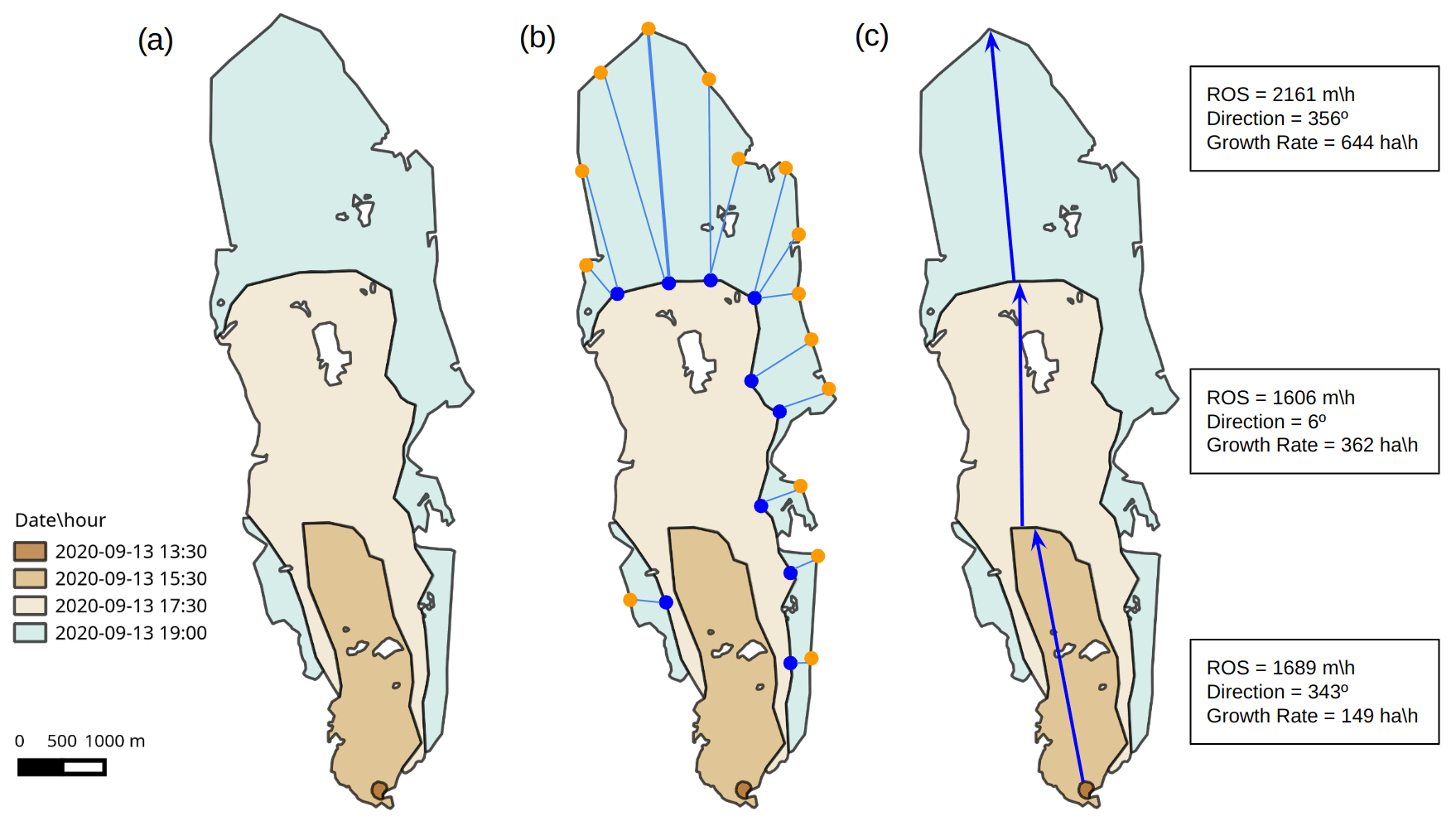
Figure 5 Example of how the fire behaviour descriptors are calculated based on the Proença-a-Nova (2020) wildfire: (a) partial fire progression, (b) procedure to calculate the distance for each vertex of the pair of consecutive polygons, and (c) estimated main spread axis and associated fire behaviour descriptors.

In addition to the standard fire behaviour descriptors, we also estimated the FRE for each progression polygon. This procedure raised additional challenges. First, MSG-SEVIRI is affected by clouds and smoke, which can hinder the estimation of FRE for some periods of the wildfires or for their entire duration. Second, due to the coarse resolution of MSG-SEVIRI, it was not possible to calculate the FRE for each polygon directly. To circumvent this, FRE was calculated for each 30 min bin from ignition until the date and/or hour of the last wildfire spread polygon. In parallel, we estimated the area burned in each spread polygon every 30 min using its start and end dates and assuming a constant FGR. Then, for each 30 min bin, the total FRE was divided by weighting its value by the proportion of area burned in each spread polygon. Finally, for each spread polygon, the 30 min FRE estimates were summed only if they covered more than 70 % of its duration (Δt_ij) to ensure that the total FRE was representative.

We also estimated the FRE flux rate (GJ ha⁻¹ h⁻¹) for each spread polygon by dividing the estimated FRE by the corresponding burned-area extent and its duration (Δt_ij). As FRE is highly dependent on the extent of burning in a given time window, the FRE flux rate can provide estimates closer to instantaneous values, which are useful for other applications.

2.5 Simplified wildfire behaviour (L3)

We calculated simplified metrics representing a mean fire behaviour across each burning period. This enables higher-level analysis of the data but at the cost of losing detail and making simplifications to the calculation of the fire behaviour metrics.

The simplified ROS corresponded to the ROSi estimated for the last spread polygon of a given burning period, i.e. the average ROS between the start and the end of each burning period. FGR was defined as the sum of the area burned in the period divided by its duration. The total FRE was calculated considering all energy released by the polygons burned within the burning period if FRE estimates covered more than 70 % of the area burned.

2.6 Quality control and quality assurance (QC/QA)

All L1 to L2 and L2 to L3 processing was done using MATLAB scripts complemented with quality control checks to identify errors in the original L1 data. These included simple checks of incorrect field names, incoherent data format (e.g. date and hour), and consistency of the fire spread structure defined by the digraphs – for example (i) the time elapsed between nodes was always positive, and (ii) every spread polygon with zp_link > 0 was always associated with a predecessor valid node (either of z or p type), among others.

During the processing of L1 data to L2, we did frequent quality checks to identify potential errors, for example, null values of ROS or FGR associated with valid fire spread polygons or fire progression polygons that did not have a known start or end date or that did not have a known link to a preceding fire source (e.g. active flaming zone). In addition, we selected some wildfires, made independent calculations of the ROS and FGR, and compared them with those estimated using the MATLAB code developed. All these quality control steps assured that the data produced were reliable and of the best possible quality. The process was iterative, requiring frequent corrections to the L1 data and re-running of the quality check.

Finally, for each wildfire, we defined a confidence flag that provides overall information on the reliability of the estimated progression data. Although directly related to L1, ultimately, it should also provide the user an estimate of the confidence associated with L2 and L3. This was defined empirically based on the uncertainties that arose in the process of building the fire progression polygons and was graded into a five-level system, where 1 refers to the lowest quality and 5 to the highest quality (Table A2).

3 Results

3.1 Overview of the PT-FireSprd database

The PT-FireSprd database contains data for 80 large wildfires that occurred between 2015 and 2021. The individual wildfire burned-area extent ranges from 250 to 45 339 ha, with a mean and median area of 5990 and 1665 ha respectively. The 80 wildfires were distributed throughout mainland Portugal, covering a wide range of environmental conditions (Fig. 6). The database spans a wide fire behaviour variability both between (e.g. Fig. 6a, b, f) and within each wildfire (e.g. Fig. 6c, e, d). The total burned-area extent of the wildfires contained in the database is around 460 000 ha, which represents about half of the area burned in the 2015–2021 period. On average, progression was reconstructed for 93 % of the area burned by the 80 wildfires, leaving 7 % deemed to be uncertain. Wildfire behaviour descriptors were estimated for 88 % of the burned-area extent (ca. 400 000 ha). The time elapsed between two consecutive fire progression polygons ranged between 30 min and 14 h 30 min, with an average value of 3 h 15 min. The mean duration of the burning periods was around 8 h, with a standard deviation of 4 h 50 min.

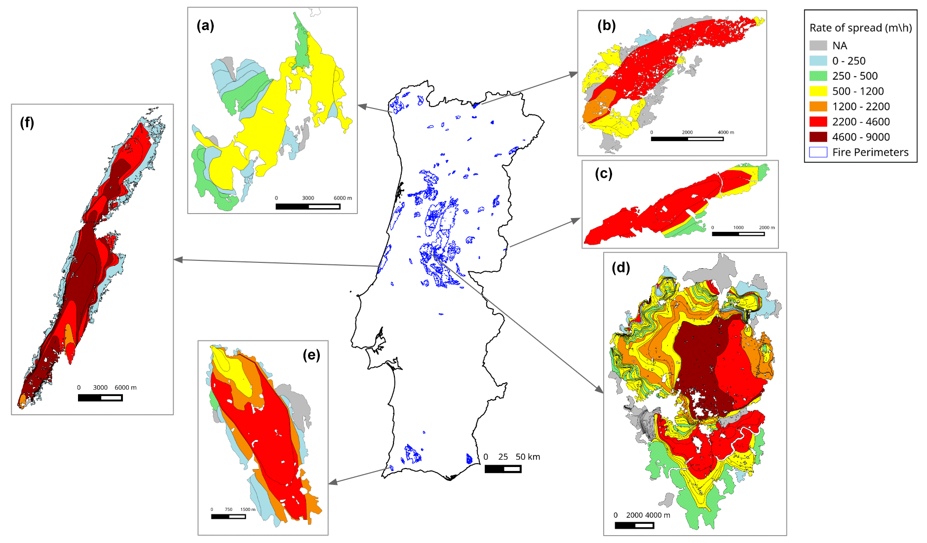
Figure 6 Overall spatial distribution of the wildfire perimeters in the PT-FireSprd database, with examples of ROS estimates for six wildfires: (a) Paredes de Coura (2016), (b) Chaves (2020), (c) Idanha-a-Nova (2020), (d) Pedrógão Grande (2017), (e) Aljezur (2020), and (f) Alcobaça (2017).

A total of 1197 polygons with ROS and FGR estimates (L2) were derived from the progression data. We excluded very small polygons (< 25 ha) from further analysis, resulting in a dataset with 874 observations. Out of the 1197 polygons, 609 had FRE estimates. Regarding L3 data, ROS and FGR were calculated for 241 burning periods (L3), and total FRE was estimated for 162 burning periods.

Overall, confidence in the database was lower for the earlier years (2015–2016) because input data were mostly from existent satellites. In 2017, the quality increased due to the integration of (i) ground data and (ii) data from 2017 large-wildfire reports. From 2018 onwards, the integration of the monitoring aircraft, the creation of the FEBMON system, and the rapid availability of all the data that flow through it significantly improved the confidence of the derived fire progressions.

The estimated forward ROS displayed a long-tail distribution (Fig. 7, in log-scale) with a median value of 341 m h⁻¹ and average ROS of 746 m h⁻¹, representing large variability (SD = 1071 m h⁻¹ and cv = 143 %, where SD and cv represent standard deviation and coefficient of variation respectively). About 20 % of the ROS values were larger than 1000 m h⁻¹, and about 9 % were larger than 2000 m h⁻¹. The maximum observed ROS was 8900 m h⁻¹ in the Lousã wildfire of October 2017. The FGR distribution was highly skewed towards low values, with median and average values of 40 and 191 ha h⁻¹ respectively (SD = 438 ha h⁻¹, cv = 228 %). About 10 % of the observations had FGR larger than 500 ha h⁻¹, and only about 5 % were larger than 1000 ha h⁻¹. The maximum observed FGR was 4400 ha h⁻¹ in the Pedrogão Grande wildfire (2017).

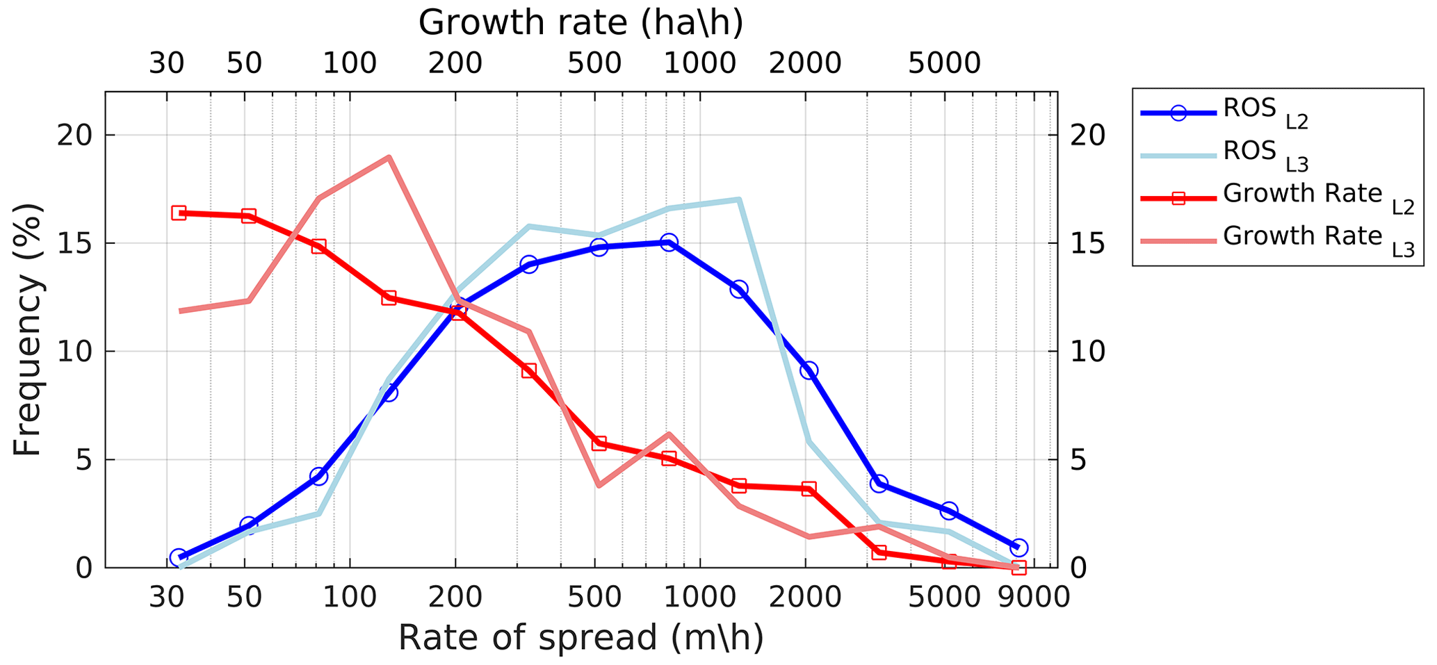
Figure 7 Estimated ROS and FGR distributions for L2 and L3 data (in log-scale). Each point represents the frequency in evenly spaced bins on a logarithmic scale.

The ROS distributions of the L2 and L3 datasets were similar. The largest differences were located in the lower and upper tails, where the L3 ROS tends to be smoother due to the averaging procedure done over a longer time span. The FGR distributions for L2 and L3 were also very similar, probably because all the polygon areas within a burning period are summed, and the value does not result from an average. Differences were larger for more complex wildfires, for example with finger run (e.g. areas resulting from rapid propagation in a different direction than the dominant fire front, often related to wind shifts).

We compared the histograms of L2 ROS and FGR for three aggregated confidence levels. The distribution of ROS estimates for wildfires with lower confidence was slightly skewed towards lower values when compared with higher confidence estimates (Fig. B1 in the Appendix). The ROS distributions peaked at 200, 500, and 800 m h⁻¹ for very-low–low, moderate, and high–very-high confidence respectively, showing a clear relationship between confidence and estimated ROS. Regarding FGR, very high values above 500 ha h⁻¹ were prevalent in wildfires with high and very high confidence progressions (Fig. B2). Results are similar if data from external reports for the extreme wildfires from June and October of 2017 are not included.

Estimated ROS and FGR were compared, and percentiles 25, 50, 75, 90, and 97.5 were calculated separately for each variable (Fig. 8). The percentile values were simplified to enable a clear communication of results, especially between researchers and fire personnel. In general, as ROS increases, so does the FGR. However, the relationship between ROS and FGR depends on the morphology of the fire perimeter: elongated fast-spreading wildfires had relatively higher ROS and lower FGR (e.g. Fig. 6b, c), while more complex burned-area perimeters had relatively lower ROS and higher FGR (e.g. a flank run with an extensive active fireline; see Fig. 6a and the last polygons of Fig. 6e and f). The data scatter tends to increase with higher ROS and FGR values, suggesting a progressively larger dependence on the burned-area extent or perimeter. Identification of the drivers behind such relationships is beyond the scope of this work. Nevertheless, wildfires at the extreme end of the distribution had very high ROS and FGR values.

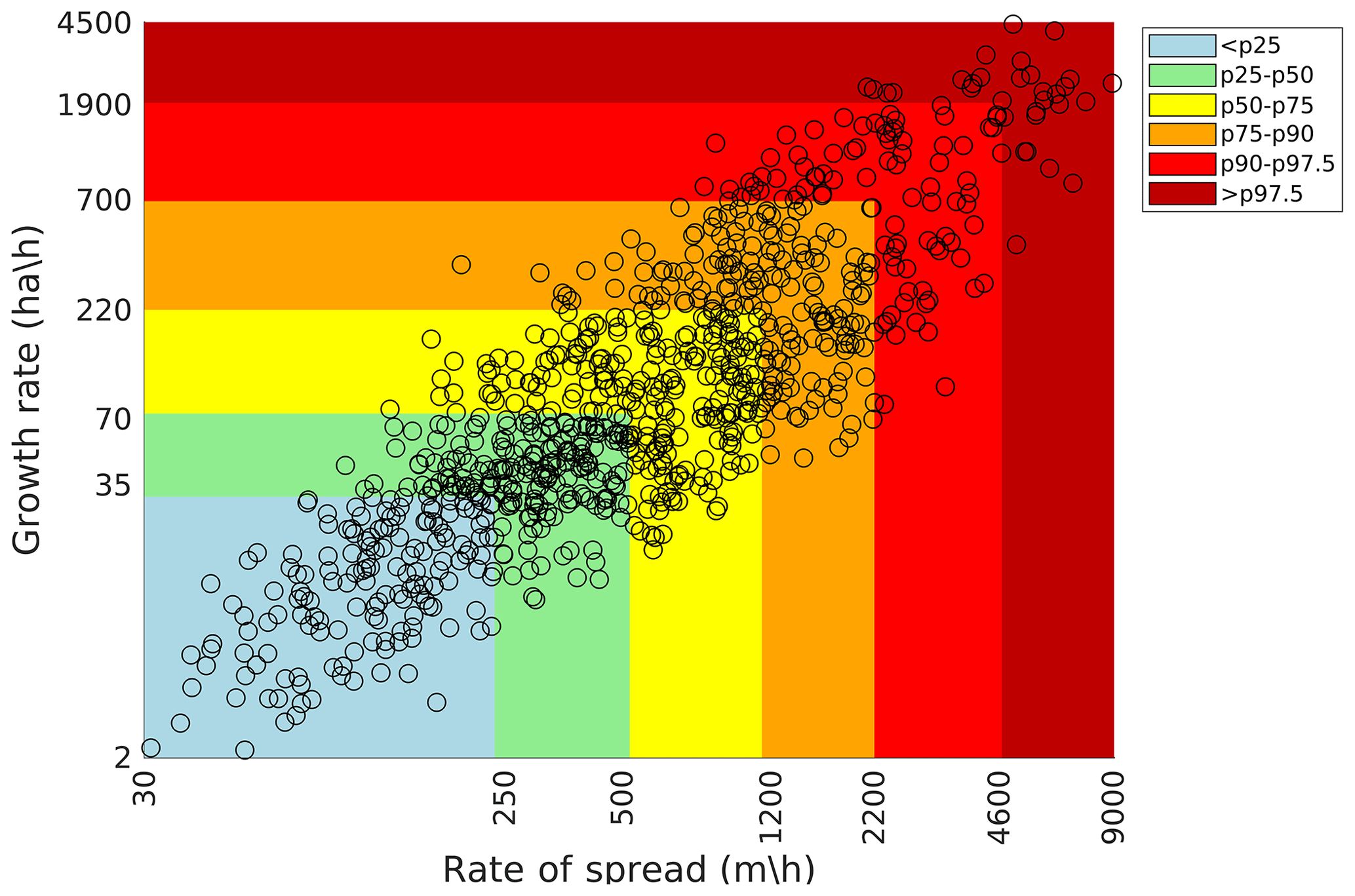
Figure 8 Distribution of the estimated partial rate of spread (ROSp) and FGR (L2). Each point represents a wildfire progression with at least 25 ha of extent. The percentiles were calculated for each variable separately (n=874). Colours represent percentile intervals for both fire behaviour descriptors.

Burned-area extent is a relevant fire behaviour descriptor for researchers and fire management personnel. Analysis shows that the area burned by a wildfire is mostly determined by its FGR (r=0.84) rather than by the speed of the forward spread (r=0.62; Fig. 9a, b). The (cor)relations were lower using L2 data. As expected, FRE is highly correlated with burned-area extent (r=0.85, Fig. 9c). Correlation between ROS and average rate of energy release (TJ h⁻¹) is lower (r=0.30, Fig. 9d), although there is a general direct relation between both descriptors.

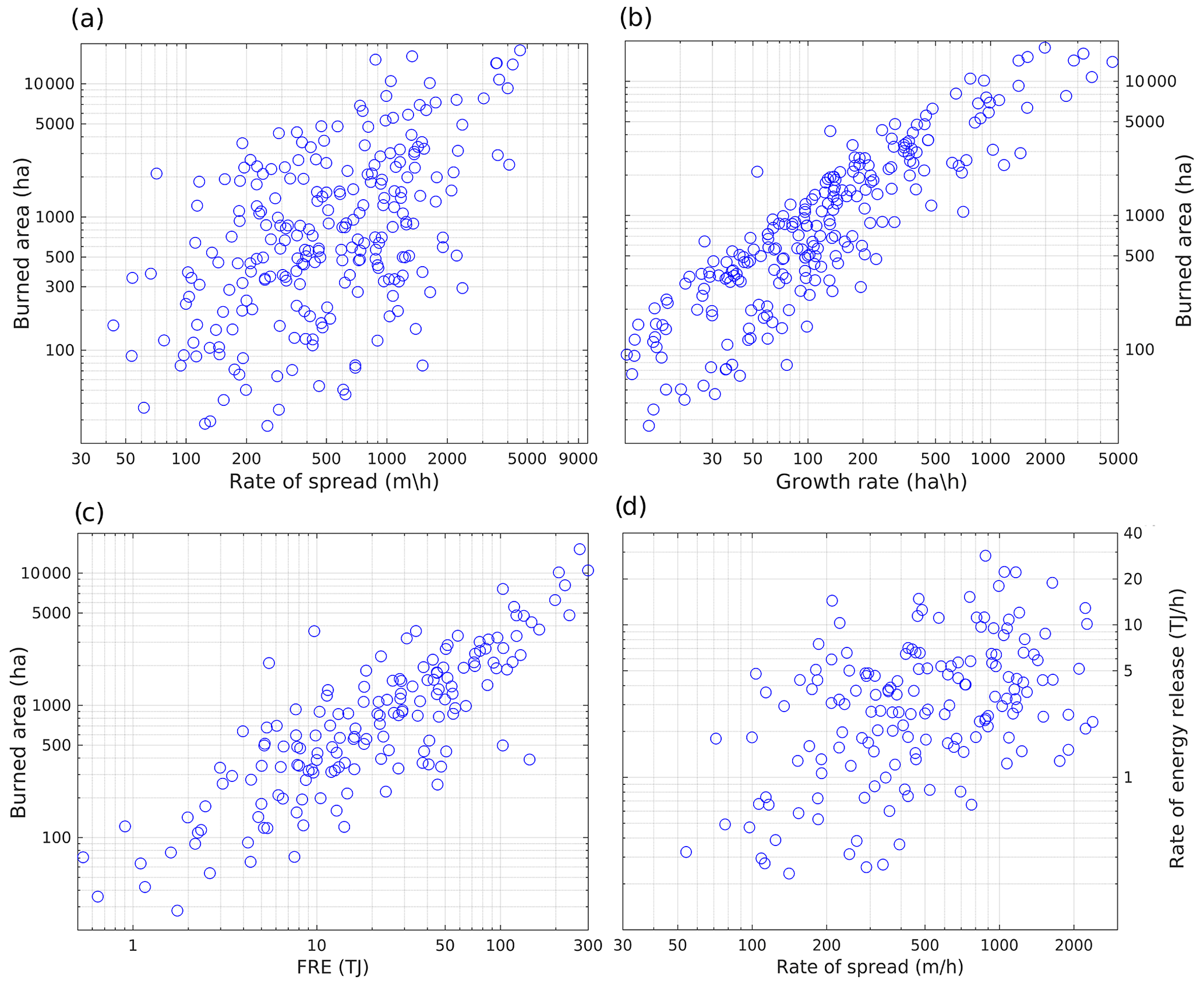
Figure 9 Comparison between simplified wildfire behaviour descriptors (L3): burned-area extent and ROS (a), burned-area extent and FGR (b), burned-area extent and FRE (c), and ROS and average rate of energy release (d). The latter was calculated by dividing the total FRE by the burning-period duration.

3.2 Case study: the Castro Marim 2021 wildfire

Here, we describe in detail the progression and behaviour of a specific wildfire to show how the PT-FireSprd database can be used, for example, to analyse case studies, which is often done by researchers and fire analysts.

The Castro Marim wildfire burned 5950 ha on 16 and 17 August 2021. Figure 10 shows its reconstructed progression (a) and associated ROS (b). Ignition occurred during the night (01:00 LT), and a single run occurred towards the southeast (SE) until approximately 08:30 LT, defined as the first burning period. The mean ROS was 618 m h⁻¹, ranging between 321 and 957 m h⁻¹ (Fig. 10c). The estimated FGR for the burning period was 43 ha h⁻¹, ranging between 33 and 77 ha h⁻¹, and the total FRE was 13 TJ (Fig. 10d).

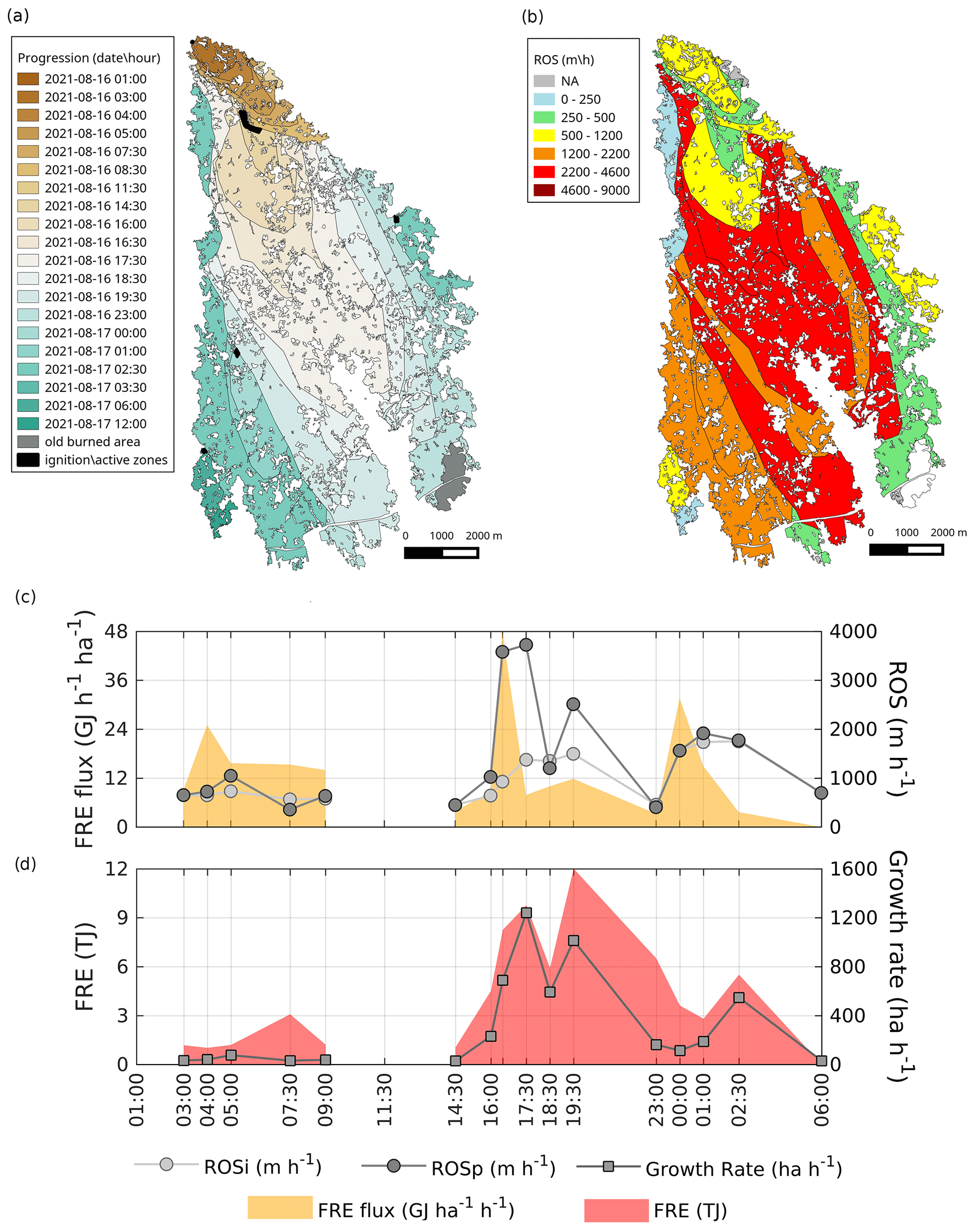
Figure 10 The Castro Marim (2021) wildfire progression (a). Wildfire behaviour descriptors include the spatial distribution of ROS (b), the temporal distribution of ROS and FRE flux rate (c), and the temporal distribution of FRE and FGR (d). Plots (c) and (d) start at 01:00 LT of 16 August and end at 06:00 LT of 17 August.

Fire progression halted for about 3 h until the wildfire reactivated around 11:30 LT. It spread southwards until the head stopped in an agricultural area around 19:30 LT. In this second burning period, fire behaviour was significantly different from the first. The mean ROS was ca. 1500 m h⁻¹, reaching a maximum value of 3720 m h⁻¹ between 16:30 and 17:30 LT. On average, the fire grew at a rate of 455 ha h⁻¹; however, significant variability was observed, with values reaching 1236 ha h⁻¹, coinciding with the ROS peak. The behaviour in the second burning period was often between percentiles 90 and 97.5. As a consequence of the behaviour exacerbation, the wildfire released around 38 TJ, with peaks of about 9 and 12 TJ observed during the afternoon. The energy flux rate was highest between 16:00 and 16:30 LT, coinciding with an abrupt increase in ROS (Fig. 10d).

After the fire head stopped, a secondary head run stopped around 23:00 LT in a previously burned area (burning period 3). In the follow-up, two left-flank runs were observed, one until 02:30 LT and the other one, resulting from a reactivation, until 06:00 LT, with decreasing ROS, FGR, and FRE. A secondary peak in the energy flux rate was estimated around 00:00 LT, associated with an increase in ROS and FGR.

Finally, in the Castro Marim wildfire, burning periods 3 and 4 overlapped in time. A progression polygon in the rear and right flank was delimited by fire personnel at 02:30 LT; however, the prior contiguous progression was identified at 16:30 LT, suggesting a very low burning flank, opposite to the fast-burning part of the wildfire southwards. This overlap had no effect on the average ROS and only a very slight effect on the estimated FGR and FRE. However, users must be aware that burning periods seldom overlap (∼ 4 % registered in the entire dataset), which may have implications in subsequent analyses.

4 Discussion

4.1 The PT-FireSprd database

The PT-FireSprd is the first open-access fire progression and behaviour database in the whole of Mediterranean Europe. The progression of 80 large wildfires that occurred in mainland Portugal between 2015–2021 is reconstructed, and fire behaviour descriptors such as ROS, FGR, and FRE are estimated, dramatically expanding the extant information (Palheiro et al., 2006; Rodriguez y Silva and Molina-Martínez 2012; Fernandes et al., 2016). Wildfire progression was derived by converging evidence from multiple data sources, which provides added reliability to the database. Wide variability in fire behaviour is covered, tackling an important limitation pointed out by Cruz (2010). The approach presented will be used to update the database in the following years for Portugal and can be replicated in other countries, depending on data availability.

The large number of fire behaviour observations, both at the polygon level (L2) and at the burning-period level (L3), provide enough information for a wide variety of potential applications. Combined with detailed information on the drivers, namely weather and fuel, and effects, it can be used to (i) improve current knowledge on the drivers affecting the behaviour of large wildfires, (ii) calibrate existing or new models which ultimately should help to better predict fire behaviour and support efficient fire management strategies (Alexander and Cruz, 2013), (iii) support the construction of case studies by fire analysts and contribute to better training of fire personnel (Alexander and Thomas, 2003), (iv) contribute to improved operational fire suppression strategies, (v) better understand how fire behaviour is linked to its effects (Collins et al., 2019), (vi) improve fire danger rating (Wotton, 2009), and (vii) better characterize fire regimes (Pereira et al., 2022). In addition, the fire behaviour classes described in Fig. 8 can assist fire suppression operations, including resource dispatches and decisions to fight or flee or offensive vs. defensive strategies.

For several reasons, it is easier to collect information for larger wildfires than for smaller ones. The wide range in fire sizes in the PT-FireSprd database suggests that it is representative of wildfires burning under a broad range of conditions. However, smaller wildfires (between 100 and 500 ha) are slightly under-represented in the database, creating a potential bias. This can be particularly relevant if one considers the high proportion of smaller wildfires that occur every year. Thus, fire behaviour descriptors may also be biased towards larger values that may have an implication, for example, for the calculated fire behaviour percentiles (Fig. 8). Note that, for typical fuel loads, say 15–20 t ha⁻¹ (Fernandes et al., 2016), ROS between percentiles 50 and 75 already corresponds to fires that are very difficult to control (Hirsch and Martell, 1996). The ROS and FRR historical distributions are a first approach with the aim of creating a simple and clear communication baseline between researchers and fire personnel based on quantitative fire behaviour data. Ultimately, the database will allow for the framing of the behaviour of new wildfires according to historical patterns. Adding smaller wildfires to the PT-FireSprd database will certainly help to better represent a wider range of fire behaviour patterns.

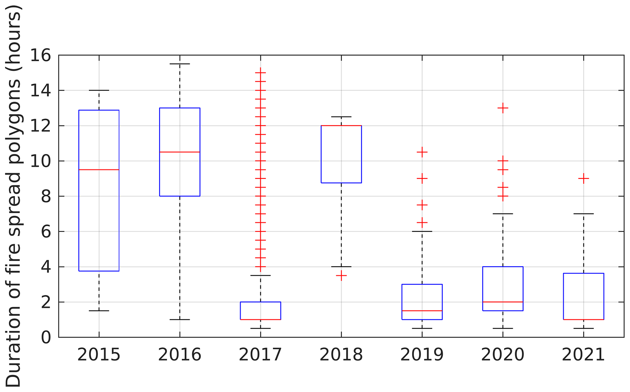
Confidence in the wildfires of 2015–2016 was lower than for the most recent ones due to relevant advances in operational fire monitoring, resulting in better-quality and higher-quantity fire data. Since 2018, the FEBMON system has improved and grown, providing larger-quantity and higher-quality data, thus leading to more reliable and detailed fire progression reconstructions. The distribution of the duration of the spread polygons between 2015 and 2021 (Fig. B3) shows heterogeneity of the database across time but also the evolution introduced along with FEBMON. Results suggest that ROS and FGR may be underestimated in wildfires with lower confidence, most probably due to the lack of sufficient data to thoroughly cover the afternoon but especially the early night period (i.e. between VIIRS and MODIS day and nighttime overpasses, Fig. 1). This issue is further discussed in Sect. 2. The user must take into account the characteristics of the database and can choose to use the entire or part of the dataset based on the confidence flag or year of the wildfire.

The PT-FireSprd database is flexible and open, allowing the users to subset the data based on their needs and requirements. For example, users can decide to work with fire behaviour descriptors at the polygon level (L2) or at the burning period (L3) or can create their own subset depending on their objectives. The dataset is heterogeneous, which is reflected in two main components: the duration of the spread polygons and the burning periods and the confidence flag associated with each wildfire.

Regarding the duration, the average time elapsed between two progression polygons was 3 h 30 min (L2) and 8 h 15 min for the burning periods (L3). Durations were large in 2015 and 2016 (median values above 9 h), decreased significantly in 2017 with the integration of hourly isochrones from Guerreiro et al. (2017, 2018), and had median durations below 2 h from 2019 (Fig. B3). Gollner et al. (2015) argued that fire progression observations need to be made in real time with a 10 m spatial resolution every 10 min to meet the needs of fire behaviour forecasting. However, in an operational context, the current objective is to predict fire behaviour time intervals larger than or equal to 30 min (Cruz and Alexander, 2013). Considering the average duration of the burning periods that represent a single fire run, the average time elapsed between progression observations represents a good compromise and a clear advance in current data. Regardless, users can subset the database based on the duration of either the progression polygons or the burning periods. L3 descriptors can be useful for providing more homogeneous and normalized fire behaviour descriptors, dampening the effect of the large variability in L2 durations, allowing, for example, a better comparison between wildfires.

Finally, results suggest that considering both ROS and FGR can improve our understanding of wildfire dynamics. The relation between both is dependent on perimeter morphology and extent (among others), and future work is needed to better understand the underlying factors. Most importantly, FGR was a better explanatory variable of burned-area extent than ROS. The practical consequence is that large burned areas can be generated by wildfires with a moderate forward ROS but with large FGR, which in turn is highly influenced by spread duration and perimeter extent. This should have implications for both the research and operational communities. FRE was estimated for a lower number of spread polygons and burning periods when compared with ROS and FGR. This was most likely due to the impact of clouds and smoke on MSG-SEVIRI detections and the conservative minimum-number-of-observations threshold (75 %). FRE and burned-area extent were closely related; however, relations between FRE and ROS were poor or moderate. One of the possible reasons may be related to the need to consider the effect of the active-perimeter extent when comparing both descriptors.

4.2 Limitations and future improvements

The generic limitations of the input data have been thoroughly described in Sect. 1. In particular, for Portugal, some limitations of the data must be pointed out. Fire progression perimeters and fire points collected on the ground by fire personnel have relevant spatio-temporal uncertainties. For example, there is often a lag between the date and/or hour a polygon is drawn in the ground and the actual date and/or hour it is burned completely. Another relevant issue is that of data acquisition and reporting errors done by fire personnel, which may be reduced by improved training and experience. The number of users of the FEBMON system has been growing in recent years, and with adequate training, it is expected that the quality and quantity of ground data will increase in upcoming years. In fact, over 27 000 aerial and 2500 ground photos were taken in the year of 2022, which represents a relevant increase compared to previous years.

Regarding airborne data, the discussion may be separated into two components. First, initial-attack photos, which can be extremely useful to draw initial fire progression and infer probable ignition areas, are not collected for every wildfire to which a helicopter is dispatched and sometimes are of poor quality. Additional training and increasing the awareness of fire personnel of the relevance of the data they collect are necessary. Second, aircraft data are acquired at relatively low altitude, precluding a synoptic view of the wildfire. Time lags between data acquisition for different parts of the wildfire (e.g. left vs. right flanks) may be large and introduce relevant spatio-temporal uncertainties in the delineation of the fire progression. In addition, perimeters are drawn manually and depend on the training and experience of the fire expert. In upcoming years, the integration of new airborne sensors, especially with multispectral capability; the ability to perform high-altitude scans; and the use of automatic perimeter delimitation procedures (e.g. Valero et al., 2018) should improve data quality and reduce the time lags of airborne fire observations. With this new capacity, it will be possible to integrate deep learning processes in the data analysis, increasing both the quantity and quality of the available fire data. This integration will also allow a well-organized structure in data collection, management, and analysis, improving decision support systems. Finally, the use of UAVs during the night (pioneered in 2022 in Portugal) will complement aeroplane and helicopter data during periods of low data availability.

Regarding official fire data, errors in the delineation of burned-area perimeters and in the ignition location, often located outside of the fire perimeter, need to be corrected to increase the quality of the PT-FireSprd database. Implementation of (semi-) automatic algorithms to delimit fire perimeters using satellite data (e.g. Chen et al., 2022) will increase data availability and reduce the uncertainties associated with manual perimeter delineation. Improvements in the spatial resolution geostationary satellites, such as the recently launched Meteosat Third Generation (MTG), will certainly improve fire behaviour estimates, as already observed from Himawari-8 and last-generation Geostationary Operational Environmental Satellite (GOES) satellites.

Concerning methodological uncertainties, the major challenge was to assign the correct date and/or hour to a specific burned area. For example, when raw data sources indicated that an area burned but active areas were absent or small, there were always uncertainties as to when it actually burned completely, which may lead to a relevant ROS and FGR underestimation. These uncertainties were larger between dusk and VIIRS overpass(es) and between the latter and dawn. One approach to reduce these uncertainties was to use FRE data to monitor the daily cycle of fire activity and to help better define the start and end dates of a progression polygon. The method was empirical, and future work is needed to better define the thresholds for setting the ignition or reactivation times, as well as the end of a fire progression. Exploratory analyses done in a few wildfires of the PT-FireSprd database suggest that FRE has a significant drop after the head of the fire stops, which may take several minutes or hours to reach the FRE thresholds used. This moment is commonly accompanied by flank growth that burns slower and releases lower amounts of energy. Such fire dynamics probably explain why ROS was likely underestimated in low-confidence wildfires and why FGR was less affected by data confidence. Improvements can be achieved in the future through the use of more sophisticated methods (e.g. change point detection), more ground observations during the head-to-flank run transition, and higher-spatial-resolution data from geostationary satellites. Part of these improvements can be used to partially update the 2015–2021 wildfires of the PT-FireSprd database.

In terms of characterizing uncertainties and their effects, future work should also adopt a metrological approach to propagate uncertainties to the descriptors, providing useful information to users. By providing an uncertainty assessment, the PT-FireSprd database would be on the pathway to Fiducial Reference Measurement (FRM) compliance (Niro et al., 2021).

The continuous update of the PT-FireSprd database will require a joint effort by researchers and fire personnel. The automation of data collection procedures (discussed above) and the dedicated training of fire personnel are key factors for guaranteeing both the quality and a sustainable update of the database. In upcoming years, other fire behaviour descriptors may be included such as type of spread (surface vs. crown fire), fireline intensity, flame length, spotting (including maximum distance), and/or pyrocumulonimbus (pyroCb) occurrence. Finally, methods described in the current work can be, at least partially, applied to many other fire-prone areas of the globe and can contribute to the much-needed data on observed wildfire behaviour.

5 Data availability

The dataset contains generic metadata files with relevant information for each wildfire (Table A3), such as the fire ID, official incident ID (ANEPC, 13-digit number), fire name, municipality, civil parish, start date, duration (h), and extent (ha), among others. The fire name was defined as Municipality_DDMMYYYY, where DD is the day, MM is the month, and YYYY is the year. In the case that more than one wildfire occurred in the same municipality on the same day, we added an additional string at the end of the fire name (e.g. _2).

The dataset is then divided into three levels in the corresponding folders:

• Fire spread (L1). Each year has a separate folder that contains one folder per wildfire labelled with the fire name. It contains a polygon shapefile with the attributes listed in Table A4.

• Fire behaviour (L2). A single polygon shapefile contains all wildfires and estimated fire behaviour metrics for each individual fire spread polygon. The attributes are listed and explained in Table A5.

• Fire behaviour (L3). A single polygon shapefile contains the simplified fire behaviour metrics calculated for each burning period. The attributes are described in Table A6.

The generic metadata are connected to L1 data through the fire name field and to L2 and L3 through the fire ID field.

The data are freely available at https://doi.org/10.5281/zenodo.7495506 (Benali et al., 2022). We intend to update the database annually with wildfires from the current fire season and implement continuous improvements to the procedure. Also, if additional information from past wildfires becomes available, we will update the database either by changing existing fire spread polygons or by adding new wildfires. Updates for future years depend on the availability of input data and associated funding.

6 Conclusions

The Portuguese Large Wildfire Spread database (PT-FireSprd) is the first open-access fire progression and behaviour database available within Mediterranean Europe. It includes the reconstruction of the progression of 80 large wildfires (> 100 ha) that occurred in mainland Portugal between 2015 and 2021, which was derived by seeking converging evidence from multiple data sources. PT-FireSprd contains a very large number of estimates of key fire behaviour descriptors, such as ROS, FGR, and FRE. Based on the statistical distribution of ROS and FGR, we defined six percentile intervals that can be easily communicated to both research and management communities and can support a wide number of applications, including better fire management strategies. The PT-FireSprd has large potential to contribute to the development of better fire behaviour prediction tools, to improve our current knowledge of wildfire dynamics, to foster better operational training, and to contribute to improved decision making. The approach will be used to continuously update the database in the following years for Portugal and can be replicated in other countries or regions, depending on data availability. Improvements in data quality and the implementation of automated methods are key factors for the regular updating of the PT-FireSprd database in the future.

Appendix A: Supporting material for the methods

Table A1 Summary of major data sources and associated characteristics.

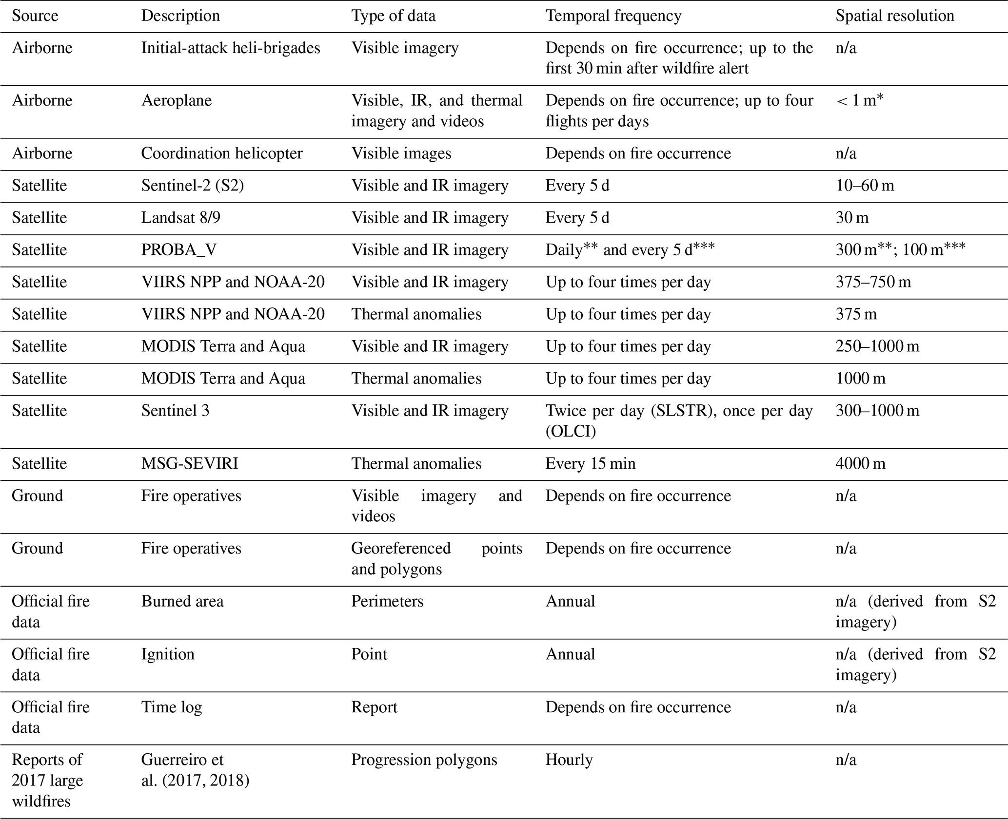
^* Depends on aeroplane flight height and on the sensor (visible sensors have higher resolution than IR sensors). n/a – not applicable

Table A2 Confidence flag value, class, and interpretation. The flag is defined for each wildfire.

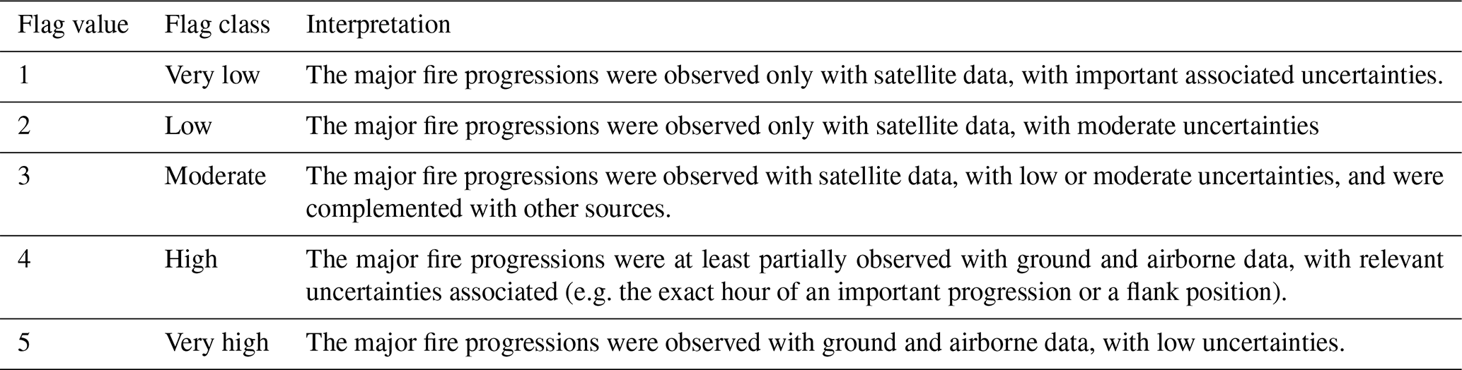
Table A3 Database metadata list for L1.

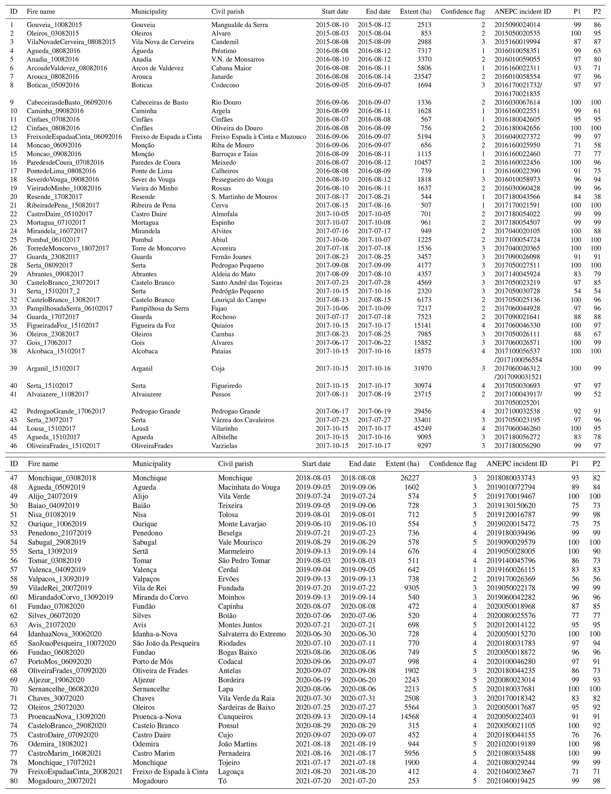
Note: p1 stands for percentage of known fire progression (%), and p2 stands for percentage of fire behaviour descriptors calculated (%).

Table A4 Attribute fields of the fire progressions (L1).

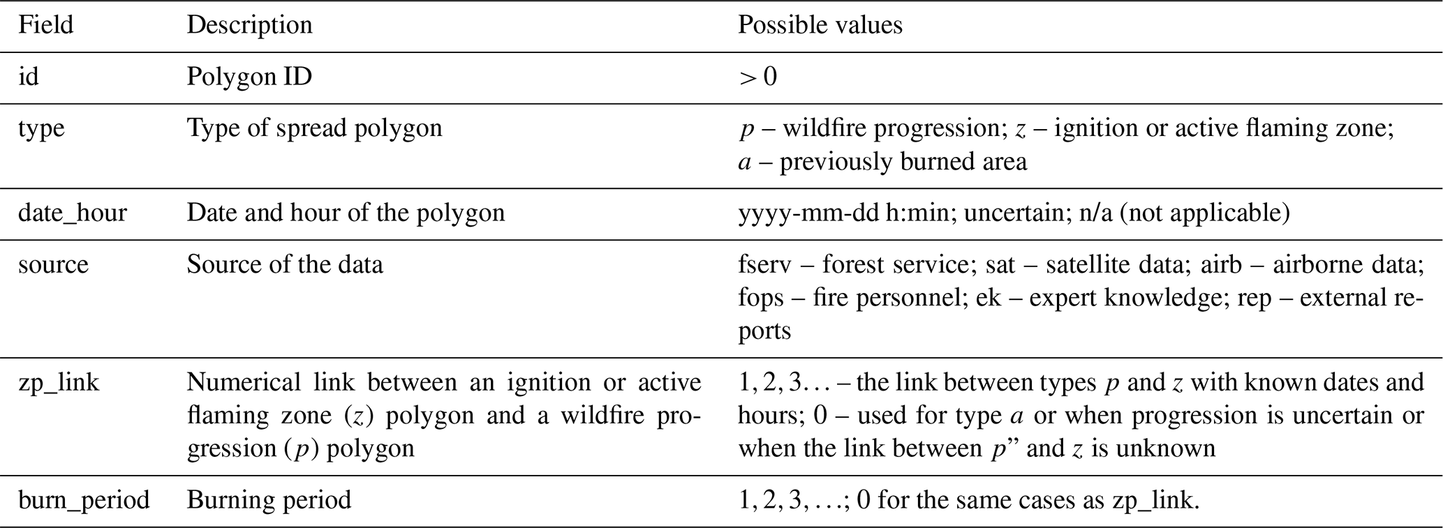
Table A5 Attribute fields of the fire behaviour database (L2).

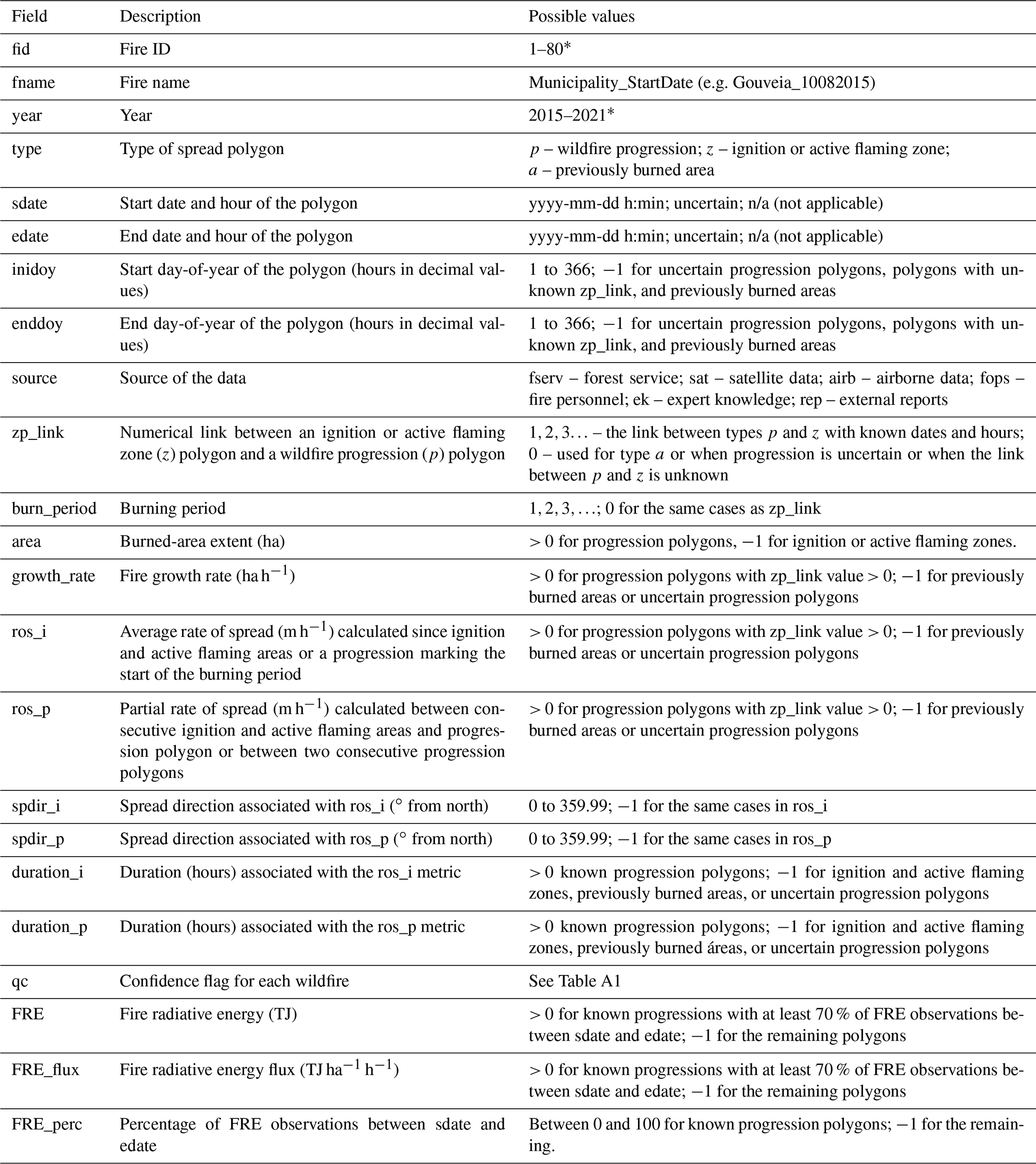
^* Values will change when the database is updated with new wildfires.

Table A6 Attribute fields of the simplified fire behaviour database (L3).

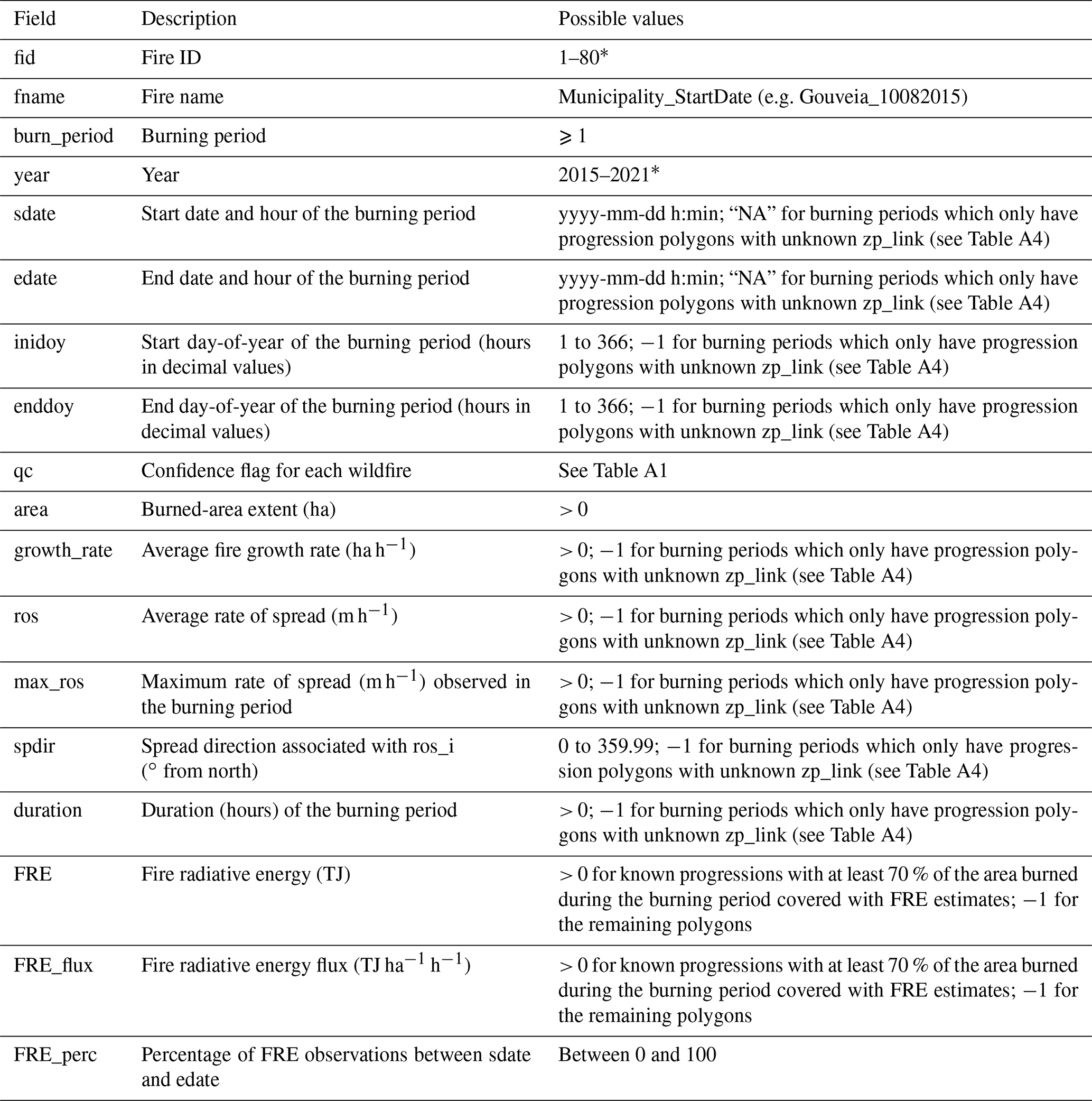
^* Values will change when the database is updated with new wildfires. NA – not available

Appendix B: Supporting material for the results

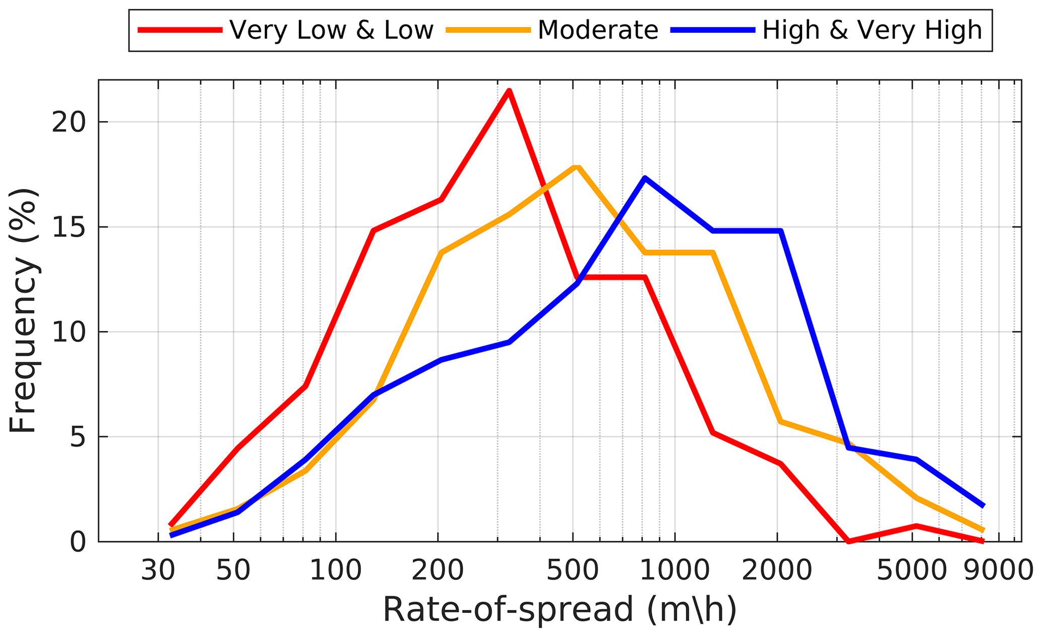
Figure B1 Histogram of the estimated ROS (L2) for three aggregated levels of confidence. L2 ROS estimates were used, and the confidence flags are explained in Table 1.

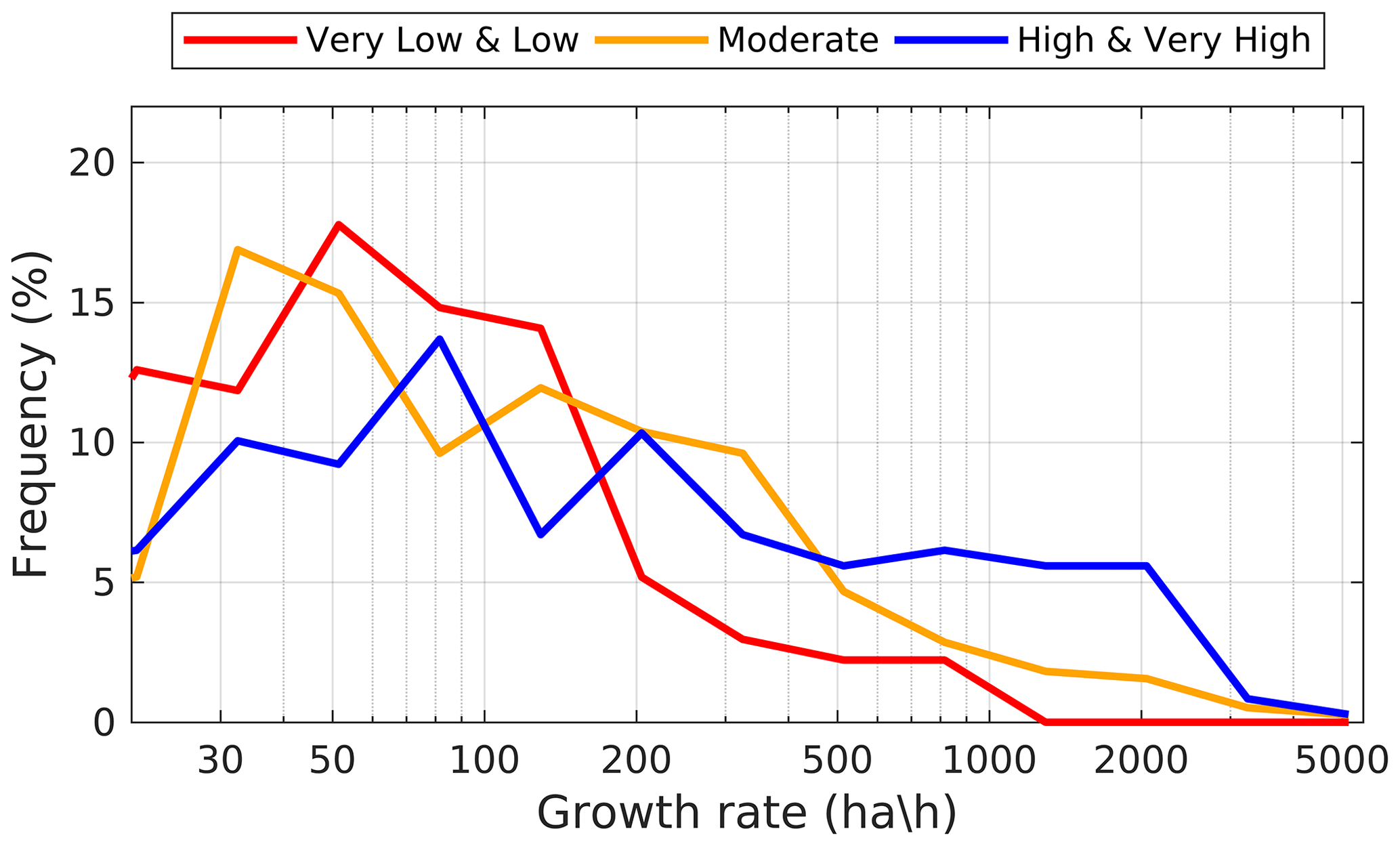
Figure B2 Histogram of the estimated FGR for three levels of confidence. L2 FGR estimates were used, and the confidence flags are explained in Table A1.

Figure B3 Distribution of the duration of the progression polygons divided by years.