the Creative Commons Attribution 4.0 License.
the Creative Commons Attribution 4.0 License.
 | 18 Aug 2023
A synthetic optical database generated by radiative transfer simulations in support of studies in ocean optics and optical remote sensing of the global ocean
Hubert Loisel
Daniel Schaffer Ferreira Jorge
Rick A. Reynolds
Dariusz Stramski
Radiative transfer (RT) simulations have long been used to study the relationships between the inherent optical properties (IOPs) of seawater and light fields within and leaving the ocean, from which ocean apparent optical properties (AOPs) can be calculated. For example, inverse models used to estimate IOPs from ocean color radiometric measurements have been developed and validated using the results of RT simulations. Here we describe the development of a new synthetic optical database based on hyperspectral RT simulations across the spectral range of near-ultraviolet to near-infrared performed with the HydroLight radiative transfer code. The key component of this development is the generation of a synthetic dataset of seawater IOPs that serves as input to RT simulations. Compared to similar developments of optical databases in the past, the present dataset of IOPs is characterized by the probability distributions of IOPs that are consistent with global distributions representative of vast areas of open-ocean pelagic environments and coastal regions, covering a broad range of optical water types. The generation of synthetic data of IOPs associated with particulate and dissolved constituents of seawater was driven largely by an extensive set of field measurements of the phytoplankton absorption coefficient collected in diverse oceanic environments. Overall, the synthetic IOP dataset consists of 3320 combinations of IOPs. Additionally, the pure seawater IOPs were assumed following recent recommendations. The RT simulations were performed using 3320 combinations of input IOPs, assuming vertical homogeneity within an infinitely deep ocean. These input IOPs were used in three simulation scenarios associated with assumptions about inelastic radiative processes in the water column (not considered in previous synthetically generated optical databases) and three simulation scenarios associated with the sun zenith angle. Specifically, the simulations were made assuming no inelastic processes, the presence of Raman scattering by water molecules, and the presence of both Raman scattering and fluorescence of chlorophyll a pigment. Fluorescence of colored dissolved organic matter was omitted from all simulations. For each of these three simulation scenarios, the simulations were made for three sun zenith angles of 0, 30, and 60∘ assuming clear skies, standard atmosphere, and a wind speed of 5 m s−1. Thus, overall 29 880 RT simulations were performed. The output results of these simulations include radiance distributions, plane and scalar irradiances, and a whole set of AOPs, including remote-sensing reflectance, vertical diffuse attenuation coefficients, and mean cosines, where all optical variables are reported in the spectral range of 350 to 750 nm at 5 nm intervals for different depths between the sea surface and 50 m. The consistency of this new synthetic database has been assessed through comparisons with in situ data and previously developed empirical relationships involving IOPs and AOPs. The database is available at the Dryad open-access repository of research data (https://doi.org/10.6076/D1630T, Loisel et al., 2023).
- Article
(5022 KB) - Full-text XML
- BibTeX
- EndNote


Investigating the propagation of natural light in the ocean can be addressed experimentally through in situ measurements and theoretically through numerical radiative transfer (RT) simulations. Understanding the relationships between the radiometric quantities (i.e., radiance and irradiances) that characterize the light fields within and leaving the ocean and the inherent optical properties (IOPs) of the water column, as well as boundary conditions at the sea surface (i.e., surface illumination conditions and sea state) and at the ocean bottom (i.e., bottom depth and albedo), requires comprehensive datasets of multiple variables acquired over a broad range of environmental conditions. For example, of particular interest are the relationships between the spectral remote-sensing reflectance of the ocean (in sr−1), Rrs(λ), which is an apparent optical property (AOP) derivable from radiometric quantities, and the seawater IOPs that are directly linked to various seawater constituents because these relationships form the cornerstone of various applications of optical (ocean color) remote sensing. Recent technological developments and broader accessibility of optical in situ instrumentation have led to a significant increase in optical datasets collected across diverse oceanic environments, and efforts have been undertaken to merge data from various sources within publicly available databases (e.g., Werdell and Bailey, 2005; Valente et al., 2019; Casey et al., 2020). Although the importance of field data collection across diverse environments cannot be overstated, existing database compilations are subject to certain limitations. In addition to typical measurement errors, it is difficult to ensure consistent data quality and characterization of uncertainties across all merged data because individual datasets are often obtained with different instruments as well as measurement and data processing methods. Also, even large databases such as NASA's SeaWiFS Bio-optical Archive and Storage System (SeaBASS, https://seabass.gsfc.nasa.gov/, last access: 1 March 2023) cannot ensure the balanced representativeness of collected field data in terms of a broad range of optical conditions across diverse ocean environments. In this context, radiative transfer (RT) simulations, which are free of measurement errors, provide a useful tool to generate comprehensive synthetic databases and complement the existing datasets of field measurements in support of studies in ocean optics and optical remote sensing.
Over the past decades, various radiative transfer models that employ different numerical solution techniques have been developed and used to address a wide range of problems related to the optics of natural water bodies (e.g., Mobley et al., 1993; Mobley, 1994; Stamnes et al., 2017). Since the 1990s, the HydroLight code based on the invariant imbedding technique (Mobley, 1989; Mobley et al., 1993; Mobley, 1994) has been among the most commonly used radiative transfer models in oceanographic optics. The HydroLight code solves the scalar (i.e., polarization of light is not included) time-independent radiative transfer equation for a horizontally homogeneous water body in which the IOPs can vary with depth and under given boundary conditions at the surface and at the bottom of the water body. Inelastic radiative processes within the water column that include Raman scattering by water molecules, fluorescence of chlorophyll a pigment, and fluorescence of colored dissolved organic matter (CDOM) can be included in HydroLight simulations.
Radiative transfer simulations with HydroLight code have proven useful for generating synthetic databases of light field characteristics (i.e., radiance and irradiances) within and leaving the ocean and the AOPs derived from the simulated radiometric quantities for various scenarios of seawater IOPs that provide input to the simulations. In particular, as a result of efforts dedicated to inverse bio-optical algorithms and coordinated under the auspices of the International Ocean Colour Coordinating Group (IOCCG Report, 2006), a widely used publicly available synthetic database was generated within the spectral range 400 to 800 nm with a 10 nm resolution for clear sky conditions with three different sun zenith angles (0, 30, and 60∘), a sea-surface state corresponding to a wind speed of 5 m s−1, and 500 different IOP combinations driven by chlorophyll a concentration, Chla (in units of mg m−3), within the surface ocean layer. The input IOP data included the spectral absorption coefficients of phytoplankton, aph(λ), non-algal particles (also referred to as depigmented or detrital particles, which can include various types of particles such as organic detritus, mineral particles, heterotrophic bacteria, and depigmented phytoplankton cells), ad(λ), colored dissolved organic matter (CDOM), ag(λ), and the spectral backscattering coefficients of phytoplankton, bb-ph(λ), and non-algal particles, bb-d(λ) (λ represents the wavelength of light in a vacuum expressed in units of nm and the IOP coefficients are typically expressed in units of m−1). The output parameters provided by simulations available in the public database included the following AOPs: spectral remote-sensing reflectance, Rrs(λ), remote-sensing reflectance just below the sea surface, rrs(λ), irradiance reflectance just below the sea surface, , and the diffuse attenuation coefficient for downwelling plane irradiance, Kd(λ,z), at the depths , 5, and 10 m (where 0− indicates a depth of just beneath the sea surface).
Another synthetic database that is publicly available was developed as part of the CoastColour Round Robin project (Nechad et al., 2015). This project was focused on coastal waters and IOPs were described by 5000 combinations of Chla, ag(λ), and the mass concentration of mineral particles. The HydroLight simulations were run from 350 to 900 nm at 5 nm intervals for a cloudless sky, three sun zenith angles (0, 40, and 60∘), and a wind speed of 5 m s−1. The output parameters included in the publicly available database are the water-leaving reflectance, RLw(λ)=πRrs(λ), Kd(λ), photosynthetically available radiation, PAR, and the euphotic depth, zeu. Most recently, a synthetic database was also developed by the first NASA PACE (Plankton, Aerosol, Cloud, ocean Ecosystem) Science Team, where the ocean contribution to top-of-atmosphere radiances were simulated by HydroLight (Craig et al., 2020). These simulations were performed from 350 to 800 nm with a 5 nm step for a cloudless sky, three sun zenith angles (10, 30, and 60∘), a wind speed of 5 m s−1, and a set of 720 IOP combinations driven by aph(λ). The publicly available output of these HydroLight simulations is Rrs(λ).
While these existing synthetic databases have provided valuable information to the ocean color radiometry (OCR) community, especially for the purpose of algorithm development where the ocean AOPs are linked to IOPs, there are several reasons that have motivated the present study, which is aimed at generating a new optical synthetic database. First, inelastic Raman scattering and fluorescence processes were ignored in the previous RT simulations. These inelastic radiative processes are known to be important for simulating realistic characteristics of light fields within and leaving the ocean, including Rrs(λ), which is a primary optical quantity used in ocean color remote sensing. For example, Raman scattering by water molecules may have an important influence on light within and leaving the ocean and AOPs, especially in the green and red parts of the spectrum (e.g., Marshall and Smith, 1990; Stavn, 1993; Sugihara et al., 1984; Westberry et al., 2013). Second, the three synthetic databases described above are based on the use of the spectral absorption, aw(λ), and scattering, bw(λ), coefficients of pure seawater in the visible part of the spectrum as defined by Pope and Fry (1997) and Morel (1974), respectively. However, more recent measurements and theoretical considerations provide new recommendations for spectral values of aw(λ) and bw(λ) (IOCCG Protocol Series, 2018; Zhang and Hu, 2009; Zhang et al., 2009). Third, the probability distributions of different IOPs that were used as input to previous RT simulations do not appear to match well with the IOP distributions observed in extensive field datasets or satellite-derived datasets representing the global ocean. This issue may have a biasing effect when the synthetic databases are used to develop optical algorithms based on AOP vs. IOP relationships, especially when the underlying goal is to represent a broad range of IOPs encountered within the global ocean, even if the primary interest is in open-ocean pelagic environments. Finally, the previous synthetic databases were developed specifically for OCR-oriented studies and publicly accessible data generally include only the surface reflectances, Rrs(λ), R(λ), rrs(λ), and Kd(λ), at selected depths. These databases do not include many of the various output variables obtained from RT simulations, such as various underwater AOPs, which can be useful in supporting a broader range of studies in ocean optics beyond ocean color remote sensing.
In this article, we present a new synthetic optical database generated using RT simulations that addresses some of the limitations of similar databases developed in the past. First, we describe the development of the synthetic IOP dataset that is required to run RT simulations. The key roles in this development are played by the measured data of the phytoplankton absorption coefficient and the desired consistency between the probability distributions of synthetic IOPs and the global distributions based on satellite observations. Following this, we describe different configurations of RT simulations that were performed with the HydroLight code. The next section is dedicated to consistency between the new optical synthetic database and in situ data, including some previously reported empirical relationships. We provide example illustrations of consistency for both the IOP and AOP data. The closing section summarizes the structure of synthetic database files and provides an example illustration of one output radiometric variable, the spectral downwelling plane irradiance, calculated with RT simulations.
2.1 General overview of methodology
The scope of the synthetic database generated with RT simulations and the degree of its representativeness of diverse marine optical environments within the global ocean depend most critically on the dataset of seawater IOPs used as input to RT simulations. In the present study, our approach to generate the IOP dataset was driven largely by the underlying goal to obtain the probability distributions of IOPs that are generally consistent with the distributions observed in the global ocean dominated by open-ocean pelagic environments. The key IOPs involved in the creation of our IOP dataset include the spectral absorption and backscattering coefficients associated with the main categories of seawater constituents representing suspended particulate matter and CDOM. Specifically, the absorption coefficients of the different constituents are the spectral absorption coefficients of phytoplankton, aph(λ), non-algal particles, ad(λ), and CDOM, ag(λ). Note that the sum represents the particulate absorption coefficient with combined contributions of phytoplankton and non-algal particles, and the sum represents the non-phytoplankton absorption coefficient with combined contributions of non-algal particles and CDOM. The backscattering coefficient of the different constituents are the spectral backscattering coefficients of phytoplankton, bb-ph(λ), and non-algal particles, bb-d(λ), such that the sum is the particulate backscattering coefficient.
Among these constituent IOPs, the phytoplankton absorption coefficient, aph(λ), plays the most fundamental role in the creation of the synthetic dataset of IOPs in this study. The aph(λ) spectra in this dataset were derived from actual measurements of phytoplankton absorption made on near-surface samples collected across diverse oceanic environments. Thus, the aph(λ) data are not “synthetic” in the sense that these data were not obtained from a modeling approach, although some spectral interpolation or extrapolation was applied to measured data as described in more detail below. In contrast, the remaining four constituent IOPs in the IOP dataset, i.e., ad(λ), ag(λ), bb-ph(λ), and bb-d(λ), are “synthetic” in the sense that they are entirely based on calculations using a modeling approach with some assumptions about the magnitude and spectral behavior of the modeled IOPs. Importantly, the measured values of aph(λ) were used in the calculations of these IOPs. These calculations are also described in detail below. Thus, each combination of the five constituent IOPs in the synthetic IOP dataset consists of the measured aph(λ) and the calculated ad(λ), ag(λ), bb-ph(λ), and bb-d(λ), where the results of these calculations depend on the measured aph(λ). As a result of this approach, it would seem justifiable to refer to the created IOP dataset as a quasi-synthetic dataset. For simplicity, however, we refer to it as a synthetic IOP dataset while bearing in mind that aph(λ) spectra were derived from measurements.
2.2 Description of the in situ dataset
Figure 1a depicts the location of oceanographic stations where the near-surface measurements of aph(λ) were made. As shown, these measurements were collected across diverse open-ocean and coastal environments. Their total number is 4382, constituting the initial field dataset of aph(λ) considered in this study. Figure 1 also shows the location of stations where coincident measurements are available for the pairs of IOP coefficients, namely aph(λ) and ag(λ) (Fig. 1b), aph(λ) and adg(λ) (Fig. 1c), and aph(λ) and bbp(λ) (Fig. 1d). We recall that while the in situ data of ag(λ), adg(λ), and bbp(λ) were not used in the development of the synthetic IOP dataset, they were assembled for the purpose of comparison with corresponding coefficients that were calculated and included in the synthetic IOP dataset. Many in situ data of the IOP coefficients used in the present study were collected in previous studies (e.g., Reynolds et al., 2001; Babin et al., 2003; Loisel et al., 2007; Claustre et al., 2008; Huot et al., 2008; Stramski et al., 2008; Lubac et al., 2008; Loisel et al., 2009; Bricaud et al., 2010; Loisel et al., 2011; Antoine et al., 2011; Neukermans et al., 2012; Uitz et al., 2015; Neukermans et al., 2016; Reynolds et al., 2016; Aurin et al., 2018; Reynolds and Stramski, 2019; Stramski et al., 2019). Some data are described in publications devoted to compilation of various datasets (Valente et al., 2019; Casey et al., 2020) and are included in several databases (e.g., SeaBASS, CoastlOOC, BOUSSOLE, and GOCAD). As the IOP coefficients in the in situ dataset were measured over a broad range of trophic and environmental conditions, their spectral values span more than 3 or 4 orders of magnitude. This large dynamic range is illustrated in terms of probability distributions at selected light wavelengths, i.e., at 440 nm for the constituent absorption coefficients and 550 nm for the particulate backscattering coefficient (Fig. 2).
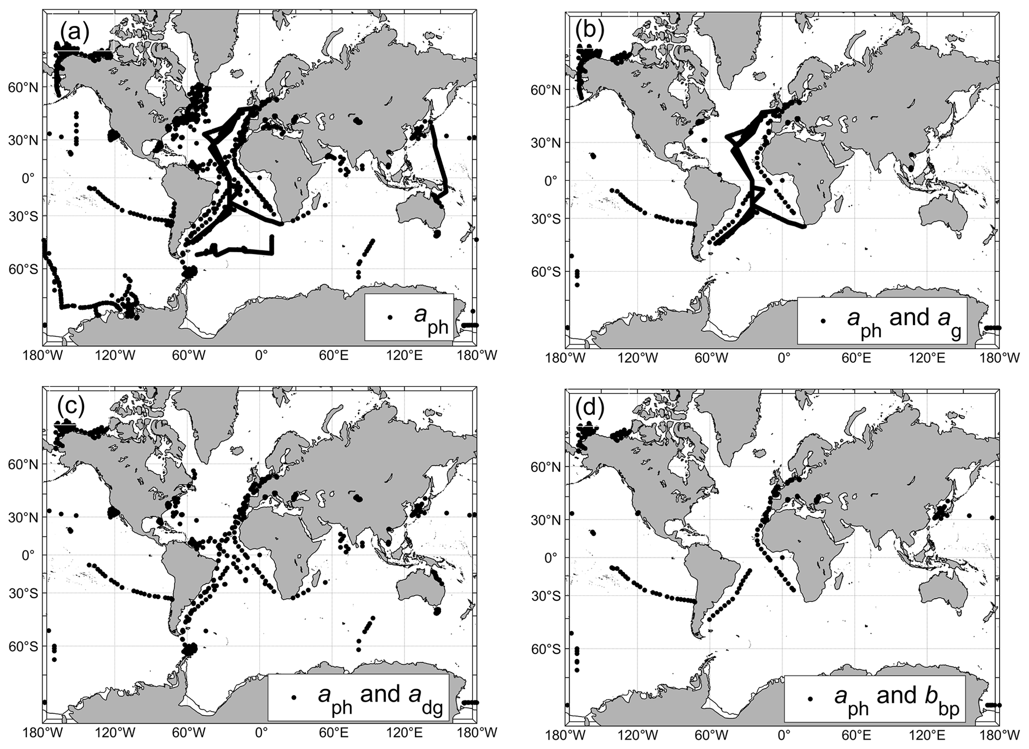
Figure 1Locations of oceanographic stations where in situ measurements were collected for (a) aph(λ), number of measurements N=4382; (b) aph(λ) and ag(λ), number of matchup measurements N=2206; (c) aph(λ) and adg(λ), number of matchup measurements N=813; and (d) aph(λ) and bbp(λ), number of matchup measurements N=775.
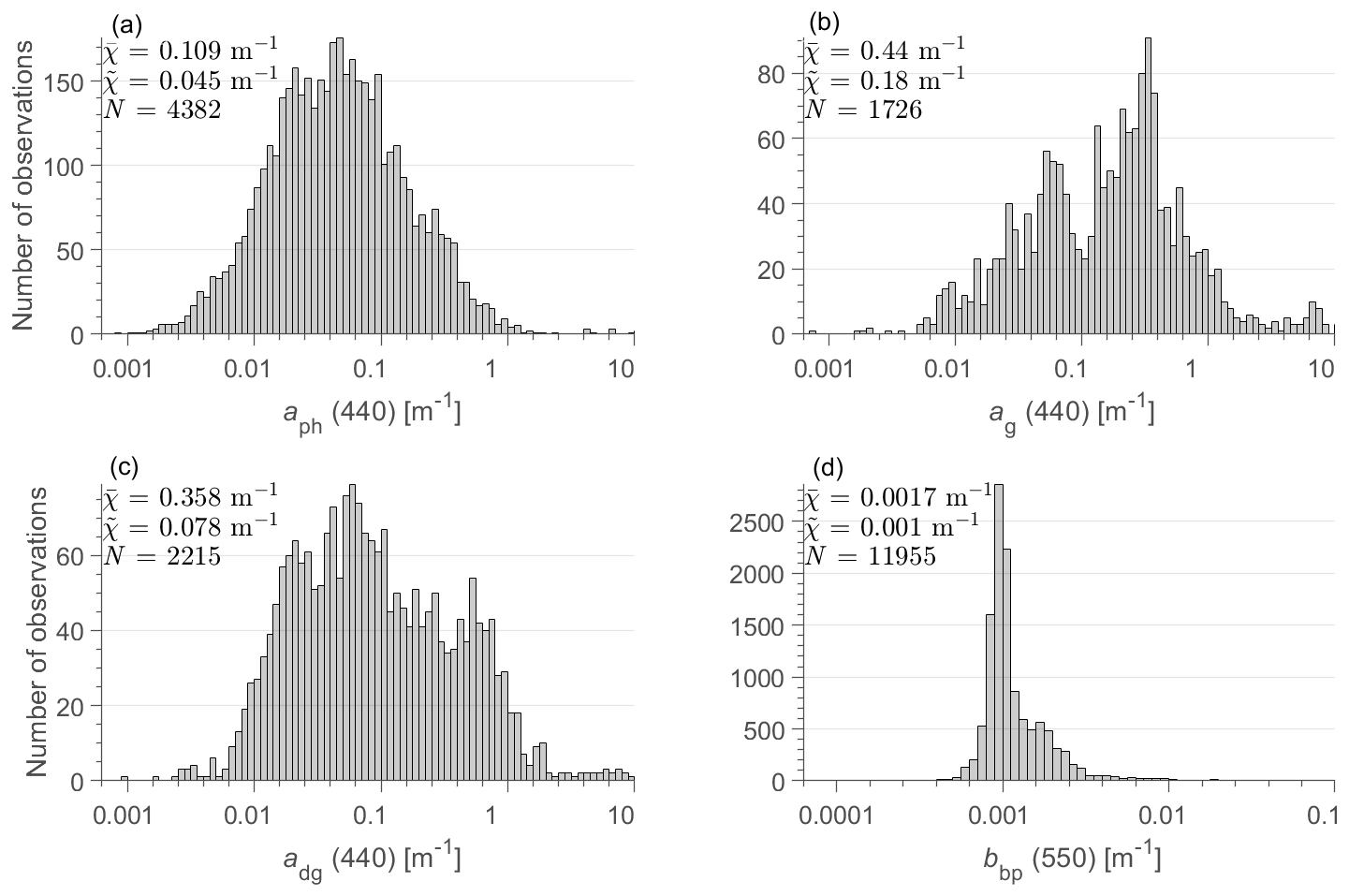
Figure 2Histograms and relevant statistical parameters of field measurements of (a) aph(440), (b) ag(440), (c) adg(440), and (d) bbp(550). N is the number of measurements, and and are the mean and median values of each IOP, respectively.
2.3 Generation of the dataset of hyperspectral aph(λ)
The first task necessary in developing the synthetic IOP dataset was to assemble data on the hyperspectral absorption coefficient of phytoplankton, aph(λ), from field measurements collected across diverse open-ocean and coastal environments (Figs. 1a, 2a). These aph(λ) data were obtained with the filter-pad spectrophotometric method as a difference between the measurements of ap(λ) and ad(λ) (Kishino et al., 1985; IOCCG Protocol Series, 2018). Historically, most of these measurements were acquired with the transmittance configuration of the filter-pad method; such measurements are included in our dataset. However, some data in our dataset were obtained with the inside integrating-sphere configuration of the filter-pad method, which is superior to the transmittance configuration of measurement (Stramski et al., 2015; IOCCG Protocol Series, 2018).
A significant portion (23.7 %) of the initial dataset of aph(λ), consisting of 4382 measurements, covers a spectral range of 400 to 750 nm with a high spectral resolution of data reported at 1 nm intervals. In some cases, the original measurements extended to the near-UV spectral region and/or longer wavelengths in the near-infrared spectral region (800 or 850 nm). The data beyond 750 nm are not used in this study because our RT simulations target the spectral range of 350 to 750 nm. It is notable that the absorption measurements of marine particles and phytoplankton are generally unavailable or are not reported in the UV because of increased methodological challenges and uncertainties in this spectral region (Stramski et al., 2015; IOCCG Protocol Series, 2018; Kostakis et al., 2021). As a result, only a relatively small fraction of aph(λ) measurements in the initial dataset were reported in the near-UV region. In addition, the initial dataset included a relatively large fraction of aph(λ) measurements that were reported at wavelength intervals larger than 1 nm. These lower-resolution data (hereafter referred to as multispectral) ranged from a small wavelength interval of 2 nm to data reported at more limited numbers of wavelengths (as few as <10) within the visible spectral range. It is likely that the multispectral data available from some data sources that we used in this study were originally measured at higher spectral resolution but were eventually reported only for some selected wavelengths, such as those corresponding to the spectral bands available on satellite ocean color sensors.
The first objective of the analysis of aph(λ) was to consider the initial aph(λ) dataset within the 400–750 nm range and convert the measurements that were reported at lower spectral resolution to uniformly hyperspectral data at 1 nm intervals. In this analysis, all measurements originally available at 1 nm intervals were considered to provide reference spectral shape functions of aph(λ). The originally multispectral data of aph(λ) were converted to hyperspectral data using several different approaches depending on the spectral features of lower-resolution data. One approach utilized the reference spectral shape functions of aph(λ) and was applied to multispectral aph(λ) data if they were reported for fewer than 100 wavelengths. In this case, a given multispectral spectrum of aph(λ) was converted to a hyperspectral spectrum using a specific hyperspectral measurement that exhibited the highest correlation with the multispectral measurement under consideration. The correlation coefficient was calculated using the spectral data available at common wavelengths of the considered pair of spectra. A necessary condition to proceed with conversion of a given multispectral spectrum to a hyperspectral spectrum was a correlation coefficient of 0.95 or higher. If this condition was satisfied, the multispectral data were converted to hyperspectral data so that the created hyperspectral spectrum maintained a multispectral measurement magnitude in the range of 440–450 nm and had the spectral shape of the reference hyperspectral measurement. An alternative approach to convert multispectral data to hyperspectral data involves a linear interpolation of multispectral data. This approach was used when the multispectral data were reported at relatively small wavelength intervals (at least 100 spectral data points available between 400 and 750 nm) or when the correlational analysis described above did not yield a correlation coefficient of 0.95 or higher (5.2 % of the multispectral data). The original multispectral spectra which did not include data below 450 nm or fell into the category of data subject to linear interpolation, but had no data above 700 nm, were rejected from further analysis. For all hyperspectral spectra that passed the above-described analysis and criteria (i.e., 2204 spectra: the 593 original hyperspectral measurements and 1611 hyperspectral spectra created from the multispectral data), the null-point correction was applied by subtracting the average value of aph(λ) in the 745–750 nm range from all spectral values in the 400–750 nm range.
The next step of the analysis was to extend all null-point corrected spectra of aph(λ) that cover the 400–750 nm range into the UV spectral region. The primary focus was on the 350–400 nm range because our RT simulations were designed to provide output results in the 350–750 nm range. For this purpose, we used a separate subset of reference hyperspectral measurements of aph(λ) that includes the near-UV spectral region. This reference subset of data consisted of 233 measurements collected across bio-optically diverse marine environments in the Pacific and Atlantic oceans and western Arctic seas. The majority of these 233 spectra (170) were collected with the inside integrating-sphere configuration of filter-pad method, while the remaining 63 measurements were done using either the transmittance or transmittance-reflectance filter-pad configuration (Zheng et al., 2014). A correlational analysis was applied to pairs of spectra, each consisting of a spectrum covering the 400–750 nm range and a reference spectrum covering the 350–750 nm range. The correlation coefficient was calculated using data at common wavelengths from the 400–750 nm range. The reference spectrum that yielded the highest correlation with the investigated 400–750 nm spectrum was selected as a basis for extrapolation of the investigated spectrum into the 350–400 nm range. This extrapolation ensured that a given investigated spectrum maintained its magnitude at 400 nm and that its extrapolated near-UV portion had the spectral shape of the selected reference spectrum. The final aspect of extrapolation in the UV is related to the spectral range 300–350 nm. The rationale for IOP data extending to 300 nm is to ensure that the results of RT simulations that start at 350 nm account for possible effects of Raman scattering by water molecules in the UV spectral region. Therefore, for the 300–350 nm range, we simply assumed that aph(λ) in this range is equal to aph(350). The limitation associated with this assumption is not considered to be serious given the limited role of the 300–350 nm range in the RT simulations and the weak Raman scattering effects in UV spectral region. Example spectra of aph(λ) in the 350–750 nm range from contrasting marine environments are presented in Fig. 3. These examples show significant variation in both the magnitude and spectral shape of aph(λ).
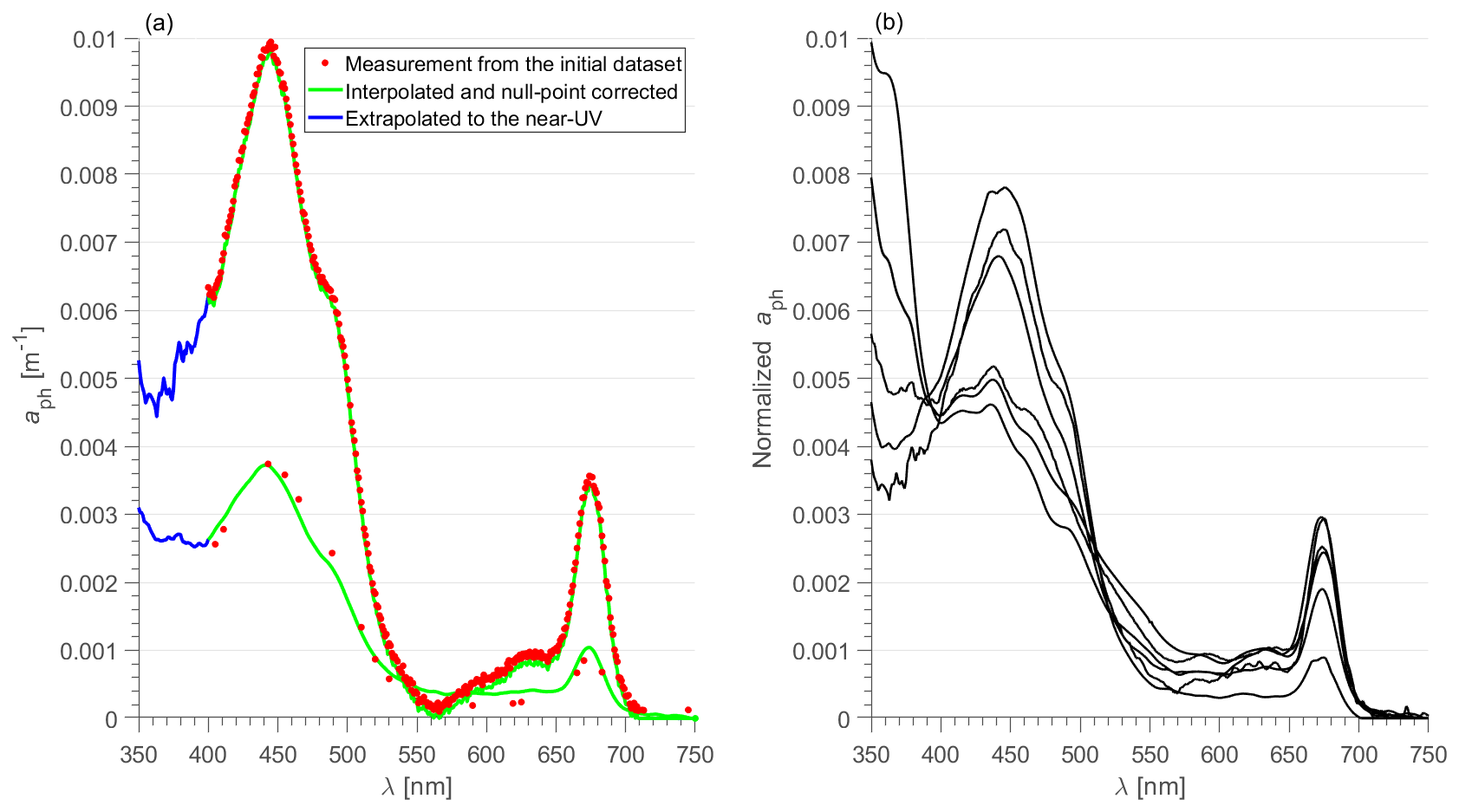
Figure 3(a) Two example spectra of aph(λ) from contrasting oceanic environments. For each example aph(λ), two spectra are displayed, namely the measurement from the initial aph(λ) dataset shown at the original wavelength intervals (red points) and the spectrum after interpolation to 1 nm intervals (if required) and null-point correction (continuous lines). The UV portion of the latter was obtained by extrapolation based on reference data in the UV (see text for details). (b) Example of normalized aph(λ) spectra illustrating the variability of the spectral shape of the aph(λ) database. These spectra have been normalized to their integral.
2.4 Generation of the complete IOP dataset
In the next step of the analysis, the subset of 2204 aph(λ) spectra that was created from the initial aph(λ) dataset as described above was subject to additional modifications to ensure that the final aph(λ) dataset was characterized by the probability distribution that resembles the distribution representative of the global ocean. This process and background information on the motivation for such adjustments in the probability distribution are described below.
When the end goal is to achieve a high degree of representativeness of the global ocean as in this study, the process of assembling in situ datasets of IOPs is unavoidably subject to limitations, even if relatively large amounts of data from many field experiments and cruises are considered. This is mainly because the global ocean is dominated by vast areas of open-ocean pelagic environments and the amount of IOP data collected in these environments is disproportionally limited compared to the amount of data collected in coastal regions, which represent a relatively small portion of the global ocean. Thus, the probability distributions based on in situ datasets, such as those presented in Fig. 2, are expected to deviate from the probability distributions representative of the global ocean. In particular, the maxima of probability distributions and the measures of central tendency, such as the median and mean values, obtained from compilations of a relatively large amount of in situ IOP data (such as in Fig. 2) are expected to be shifted to larger values compared to actual global distributions because the IOPs exhibit a general tendency of higher values in coastal regions compared to open-ocean environments. While this issue has been recognized, it has not been addressed or resolved in various studies that focus on global ocean color applications. For example, current global ocean color algorithms for estimating chlorophyll a concentration (Chla) are based on relatively large amounts of in situ data whose probability distribution is shifted significantly to higher Chla compared with the global Chla distribution (O'Reilly and Werdell, 2019). Similarly, in the development of previous synthetic optical databases with RT simulations (e.g., IOCCG Report, 2006), no special attempt was made to ensure consistency between the probability distributions of input IOP data and the distributions expected for the global ocean. In the recent development of refined global ocean color algorithms for estimating the concentration of particulate organic carbon (POC), the in situ dataset was assembled with a goal to achieve reasonable consistency with a global POC distribution (Stramski et al., 2022). This goal was, however, achieved at the expense of a significant reduction in the amount of accepted in situ data compared to the size of the overall pool of available in situ data.
In this study, our goal was to create a relatively large synthetic IOP dataset based on the initial dataset of several thousand measurements of spectral aph(λ) so that the probability distributions of IOPs in the final synthetic dataset are reasonably consistent with the expected distributions representative of the global ocean. As described above, the initial field dataset in support of this process consisted of 4382 spectra of aph(λ); this number was further reduced to 2204 spectra that were accepted as a result of analysis and some criteria applied to the initial dataset. This reduced dataset of accepted aph(λ) spectra was then further modified to ensure that the final probability distribution of aph(440) resembles the global distribution of aph(440). The global probability distribution of aph(440) was estimated using retrievals of aph(440) from satellite ocean color data. Specifically, we used global satellite observations made with the ocean color sensor OLCI (Ocean and Land Colour Instrument) deployed on the Sentinel-3 mission (Donlon et al., 2012) from the period 1 December 2020 through 30 November 2021. The weekly data product of remote-sensing reflectance Rrs(λ) at 4 km2 spatial resolution was used as input to the three-step semi-analytical algorithm (3SAA) to derive aph(443) as described in Jorge et al. (2021). The adg(443) and bbp(λ) coefficients were also derived from this algorithm. In general, the 3SAA first derives the diffuse attenuation coefficient for downwelling plane irradiance averaged within the surface layer down to the first attenuation depth, 〈Kd(λ)〉1, from Rrs(λ), and then utilizes the inverse model LS2 (Loisel et al., 2018) to derive the total absorption, a(λ), and backscattering, bb(λ), coefficients from Rrs(λ) and 〈Kd(λ)〉1. After subtracting the pure seawater contributions, the non-water absorption, anw(λ), and the particulate backscattering, bbp(λ), coefficients are obtained. Finally, aph(λ) and adg(λ) are derived from anw(λ) using an optimization algorithm of Zhang et al. (2015) with modifications that account for differences in optical water types defined in terms of different spectral shapes of Rrs(λ) (Mélin and Vantrepotte, 2015). While the original classification of Mélin and Vantrepotte (2015) includes 16 optical water classes (OWCs), the derivation of aph(λ) and adg(λ) from the 3SAA additionally included a 17th OWC to improve the representation of ultra-oligotrophic waters such as those found in the South Pacific Gyre (Morel et al., 2007; Claustre et al., 2008; Stramski et al., 2008) and in some areas of the Mediterranean Sea in summer (Loisel et al., 2011). This 17th OWC is described in Jorge et al. (2021).
The 3SAA does not yield the separate contributions of CDOM, ag(λ), and non-algal particles, ad(λ), to the overall non-phytoplankton absorption coefficient, adg(λ). Therefore, we also used another semi-analytical model (CDOM-KD2) described in Bonelli et al. (2021) to estimate ag(443) from OLCI-derived Rrs(λ). Having adg(λ) from the 3SAA and ag(λ) from CDOM-KD2, non-algal particulate absorption, ad(λ), was obtained as the difference adg(λ)−ag(λ). As a result of this analysis, we obtained a dataset of satellite-derived constituent absorption coefficients, aph(443), ag(443), ad(443), and adg(443), as well as the particulate backscattering coefficient, bbp(550), where we focused on the spectral band near 440 nm for absorption and 550 nm for backscattering.
For illustrative purposes, Fig. 4a depicts the spatial distribution of 17 optical water classes (OWCs) over the global ocean obtained from satellite OLCI data following the methodology of Mélin and Vantrepotte (2015). For further illustrative purposes, these 17 OWCs were grouped into three optical water groups (OWGs). Group 1 consists of OWC1 and OWC2, which are characterized by high water turbidity such as in coastal areas affected by discharge from large rivers. Although the focus of this study is to create synthetic datasets representative primarily of open ocean and moderately turbid coastal waters, an explicit identification of Group 1 data that represent very turbid waters is of interest for comparisons with the database developed specifically for coastal waters by Nechad et al. (2015). The second OWG, Group 2, includes six OWCs: from OWC3 through OWC8. This group represents mainly productive waters in both coastal and open-ocean environments, such as those encountered in the North Atlantic during phytoplankton bloom periods (Lévy et al., 2005). Finally, Group 3 included the remaining nine OWCs: from OWC9 through OWC17. These water types are observed mainly in mesotrophic and oligotrophic regions of the global ocean. Based on this classification, 79.6 % of OLCI water pixels in Fig. 4a belong to Group 3, 10.8 % to Group 2, and 9.6 % to Group 1. The histograms of OLCI-derived Rrs(443) associated with these three groups of data are shown in Fig. 4b. For comparative purposes we also assembled a dataset of in situ measurements of Rrs(λ), which were collected at various locations within the global ocean (Fig. 4c). The histograms of in situ Rrs(443) associated with Groups 1, 2, and 3 are depicted in Fig. 4d, which show a similar pattern to that in Fig. 4b. For the in situ dataset of Rrs(λ), 69.2 % of data belong to Group 3, 15.7 % to Group 2, and 15.1 % to Group 1.
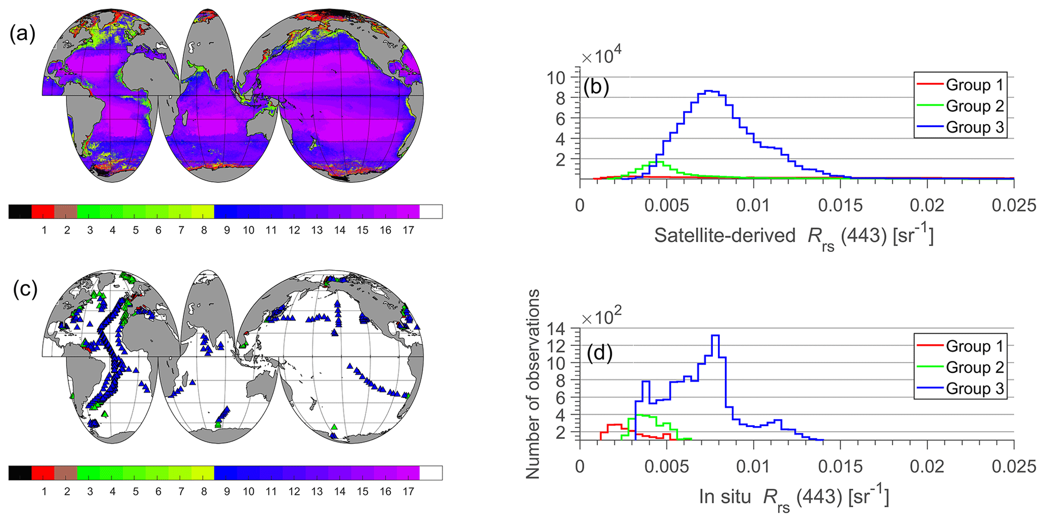
Figure 4(a) Global map illustrating the distribution of 17 optical water classes estimated from monthly Rrs(λ) values derived from satellite observations with the ocean color sensor OLCI from December 2020 through November 2021 (weekly products at 4 km2). The color bar scale refers to optical water classes. (b) Histogram of OLCI-derived Rrs(443) for the three optical water groups (see text for details). (c) Location of oceanographic stations where in situ measurements of Rrs(λ) were collected and used to analyze the consistency of the synthetic dataset with field measurements. (d) Histograms of in situ measurements of Rrs(443) for the three optical water groups.
The probability density functions (PDFs) of global satellite-derived aph(440), ag(440), adg(440), and bbp(550) are depicted in Fig. 5. We refer here to satellite-derived absorption coefficients at 440 nm although they were derived from OLCI reflectances at 443 nm, which is a minor difference that is inconsequential for the purpose of this study. Comparison of Figs. 2a and 5a indicates that the distribution of measured aph(440) from our initial field dataset (Fig. 2a) is shifted towards higher values compared to the global distribution of satellite-derived aph(440) (Fig. 5a). The probability distribution of reduced dataset of measured aph(440) (N=2204) that was created from the initial field dataset of aph(λ) shows similar deviations from the global distribution (not shown). Thus, to create the final dataset of aph(λ) that has the probability distribution of aph(440) consistent with the global satellite-derived distribution, we adjusted the number of aph(440) measurements in each bin of the histogram of the reduced dataset either by removing the measurements from any given bin or by adding the measurements to this bin. The removal or addition of aph(440) measurements associated with any given bin was done by subjecting all aph(440) measurements originally contained within a given bin to random selection. Specifically, in the case of addition the randomly selected aph(440) was added as a replicate of aph(440) to a given bin. In the case of removal, the randomly selected aph(440) was simply removed from a given bin. As a result of this process, we obtained a modified distribution of measured aph(440) that is fairly consistent with the satellite-derived distribution of aph(440). Both the modified histogram and the corresponding modified PDF of measured aph(440) are depicted in Fig. 5a for comparison with the global satellite-derived distribution. In total, this modified distribution consists of 3320 measurements of aph(440); obviously, each of these measurements at 440 nm has an associated full spectrum of aph(λ) values between 300 and 750 nm. These 3320 spectra of aph(λ) represent one IOP component of the final synthetic IOP dataset.
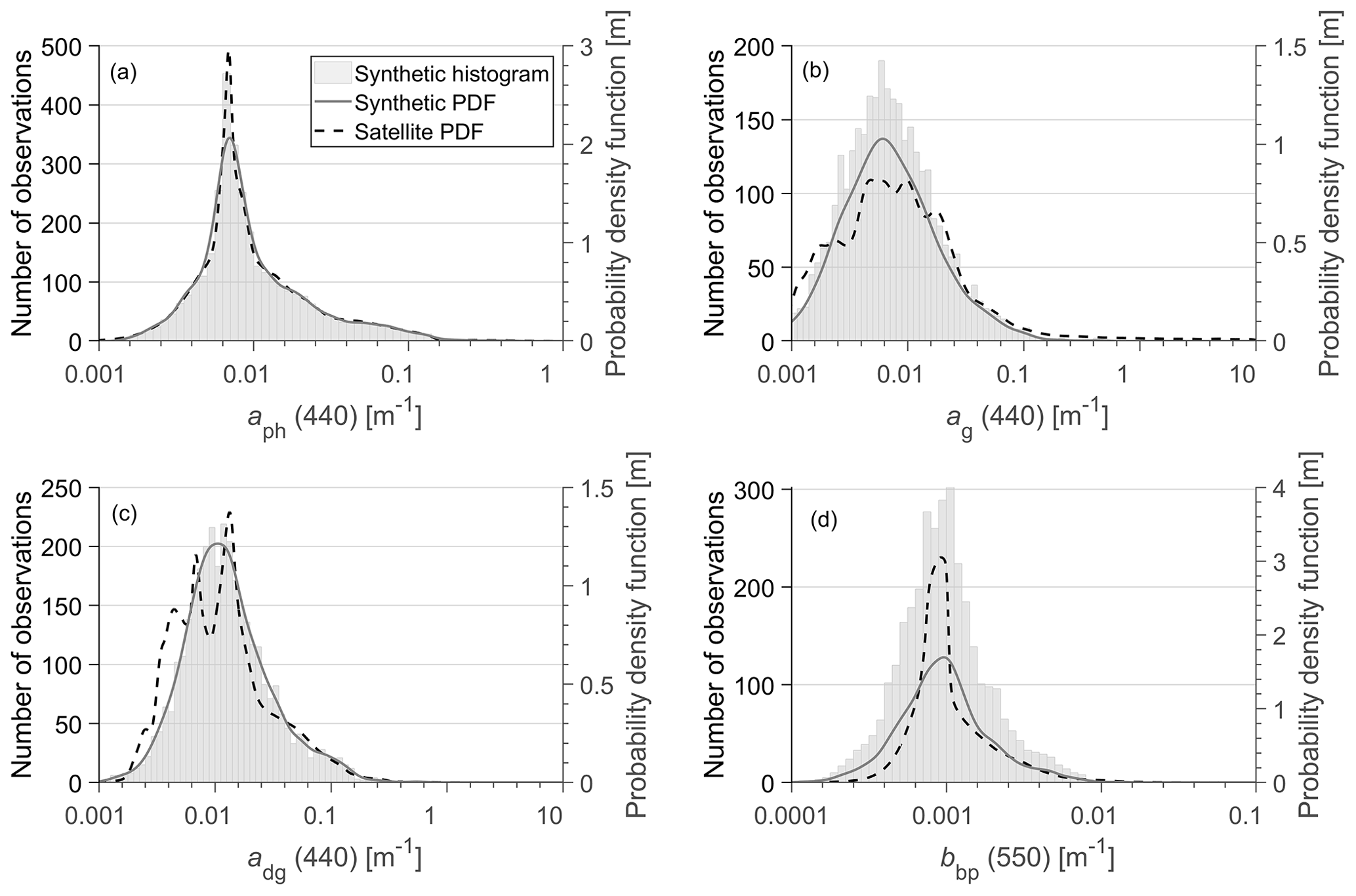
Figure 5Histograms showing the distribution of the synthetic IOP data used in the present study. The synthetic and satellite-derived probability density functions (PDFs) for each IOP are represented by the solid and dashed curves, respectively.
The full synthetic IOP dataset created in this study consists of 3320 combinations of measured aph(λ) and synthetically generated ad(λ), ag(λ), bb-ph(λ), and bb-d(λ). Below is a description of calculations of ag(λ), ad(λ), bb-ph(λ), and bb-d(λ). We note that all IOP coefficients are expressed in units of m−1 and the light wavelength is given in nanometers.
The four IOP coefficients were calculated using a similar methodology to that applied in previous studies aiming at generation of synthetic ocean optical databases (IOCCG Report, 2006; Craig et al., 2020). Specifically, we used the measured values of aph(440) as the main driver of calculations of ag(λ), ad(λ), bb-ph(λ), and bb-d(λ). Thus, the variability in the measured aph(440), as depicted by the probability distribution of measured aph(440) in Fig. 5a, is the main source of variability in these four co-existing IOP coefficients. It is notable that the replicate values of aph(440) present within any given bin of the aph(440) distribution result in the generation of different values of the four IOP coefficients because the formulas involved in these calculations contain random parameters. The coupling between aph(440) and CDOM absorption coefficient was defined as
where P1 is a parameter related to aph(440) and γ is randomly selected from a predetermined range of values (Table 1). The spectral values of ag(λ) are subsequently determined from
where the spectral slope parameter, Sg in units of nm−1, is randomly selected from a predetermined range of values (Table 1). The absorption coefficient of non-algal particles was modeled in a similar fashion:
where P2 is a parameter related to aph(440) and the spectral slope parameter Sd (nm−1) is randomly selected from a predetermined range of values (Table 1). The parameterizations of P1 and P2 were chosen to match relationships observed in the in situ dataset assembled in this study.
Table 1Symbols of variables, mathematical expressions, and corresponding equations in the text of the paper. rng(0,1) is a random number between 0 and 1.
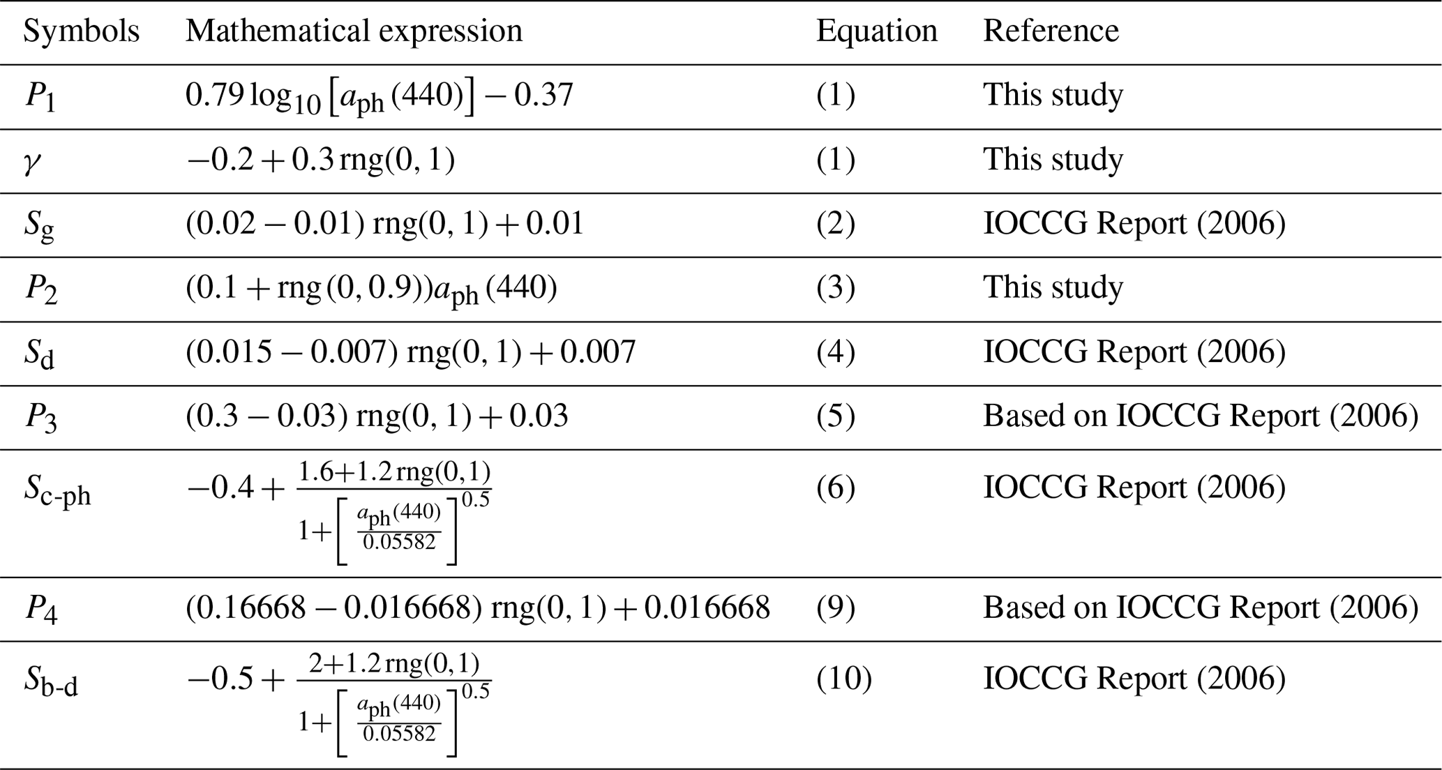
Particulate backscattering is not modeled in terms of the single coefficient bbp(λ) but instead as separate contributions by phytoplankton, bb-ph(λ), and non-algal particles, bb-d(λ), so that their sum yields bbp(λ). In order to calculate bb-ph(λ), first the formula that couples aph(440) with the beam attenuation coefficient of phytoplankton at 550 nm, cph(550), is used:
where Chla is the concentration of chlorophyll a in units of mg m−3, 0.05582 (m2 mg−1) is the value of chlorophyll-specific absorption coefficient of phytoplankton at 440 nm, (Maritorena et al., 2002), and P3 is a parameter with a randomly selected value from a predetermined range (Table 1). The exponent value of 0.57 is based on the study of Voss (1992). Subsequently, the spectral values of phytoplankton beam attenuation coefficient are calculated from
where the spectral slope parameter, Sc-ph (dimensionless), is calculated using both aph(440) and a random number generator (Table 1). Next, the spectral scattering coefficient of phytoplankton is determined:
where the spectral values of aph(λ) are from the same measured spectrum as the value of aph(440) in Eq. (5). Finally, the spectral backscattering coefficient of phytoplankton is calculated from
where 0.01 is the value of the backscattering ratio of phytoplankton, , assumed to be constant and independent of the light wavelength in the present study (IOCCG, 2006; Loisel et al., 2007). Laboratory measurements performed on various phytoplankton cultures have shown, however, that can exhibit a slight spectral variation, with the value at 442 nm ranging from 0.0035 to 0.029 (Whitmire et al., 2010). We note that bb-ph(λ) is not required as input to our radiative transfer simulations but bph(λ) is needed.
To calculate the backscattering coefficient of non-algal particles, bb-d(λ), phytoplankton absorption at 440 nm is first coupled with the scattering coefficient of non-algal particles at 550 nm, bd(550), using the following relationship:
where the parameter P4 is randomly selected from a predetermined range (Table 1) and the value of 0.05582 is as explained in relation to Eq. (5). The exponent value of 0.766 is based on the study of Loisel and Morel (1998). Then, the spectral values of non-algal scattering coefficient are calculated from
where the spectral slope parameter, Sb-d (dimensionless), is calculated using both aph(440) and a random number generator (Table 1). In the final step, the spectral backscattering coefficient of non-algal particles is calculated as
where the constant 0.018 is the backscattering ratio of non-algal particles, . This value was proposed by Mobley (1994) and was derived by averaging three particle phase functions measured in oceanic waters by Petzold (1972). Again, we note that bb-d(λ) is not required as input to radiative transfer simulations but bd(λ) is needed. The spectral slope of bbp(λ), γ, where bbp(λ) is obtained as the sum of bb-ph(λ) and bb-d(λ), has a mean and standard deviation of −1.10 ± 0.34 and exhibits a trend from oligotrophic (where γ is around −2) to eutrophic waters (where the bbp(λ) spectrum is nearly flat). These results are in good agreement with previous studies (Morel and Maritorena, 2001; Loisel et al., 2006; Antoine et al., 2011).
The variability of measured aph(440) illustrated in Fig. 5a, along with the dynamic range of parameters P1, P2, P3, P4, the spectral slopes Sg, Sd, Sc-ph, and Sb-d, and the degree of randomness in the selection of these parameters for any given value of aph(440) that initiates the process of calculating ag(λ), ad(λ), bb-ph(λ), and bb-d(λ), resulted in the generation of the synthetic dataset of IOP coefficients covering a wide dynamic range consistent with in situ and satellite observations over the global ocean. Figure 5b, c, and d compare the probability distributions of satellite-derived ag(440), adg(440), and bbp(550) with the distribution of these coefficients from the final synthetic IOP dataset. This comparison supports the general consistency of the distributions of these IOP coefficients, which is in line with the desired consistency achieved for aph(440) (Fig. 5a) as discussed earlier in this section. It is also noteworthy that in contrast to this newly created synthetic IOP dataset, the previous synthetic datasets exhibit significant differences between the probability distributions of synthetic IOPs and global distributions based on satellite observations (Fig. 6).
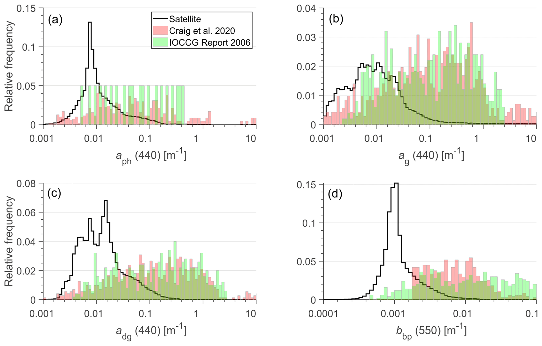
Figure 6Histograms showing the distribution of IOPs from the synthetic datasets of the IOCCG Report (2006) and Craig et al. (2020) in green and pink, respectively. The IOP distributions estimated from satellite ocean color observations by the OLCI sensor over the global ocean are represented by the black line.
Overall, the above-described synthetic IOP dataset includes 3320 scenarios of non-water IOPs, i.e., IOPs associated with the variable contributions of phytoplankton, non-algal particles, and CDOM to the optical properties of seawater. In addition to the non-water absorption coefficients, aph(λ), ad(λ), and ag(λ), as well as the non-water scattering coefficients, bph(λ) and bd(λ), the radiative transfer simulations required input of scattering phase functions of particles, specifically for phytoplankton and non-algal particles. We assumed the particulate phase functions proposed by Fournier-Forand (1994) with the backscattering ratio for phytoplankton and for non-algal particles. Note that while the backscattering ratios are assumed to be spectrally constant, the phase functions vary with light wavelength because of spectral variations of bph(λ) and bd(λ). All IOP data in the final synthetic IOP dataset cover the spectral range of 300 to 750 nm with a 5 nm interval. This wavelength interval is consistent with the intended output of our radiative transfer simulations.
The radiative transfer simulations also required input of the absorption and scattering properties of pure seawater. For the spectral absorption coefficient of pure seawater, aw(λ), we used the values recommended in the IOCCG Protocol Series (2018). This recommendation includes the values from Jonasz and Fournier (2007) for the spectral range 300–330 nm, Morel et al. (2007) for 340–415 nm, Pope and Fry (1997) for 420–725 nm, and Kou et al. (1993) for 730–750 nm. The spectral volume scattering function of pure seawater (from which the spectral scattering coefficient and scattering phase function can be obtained) was calculated following Zhang et al. (2009), assuming a water temperature of 18 ∘C and a salinity of 35 ‰. The temperature of 18 ∘C is consistent with the mean sea-surface temperature (SST) calculated from the monthly global NOAAv2 SST database at 1∘ spatial resolution from December 1991 through November 2021 (Jérôme Vialard, personal communication, 2023). The salinity of 35 ‰ is also consistent with the global surface average (Durack et al., 2013).
The IOP dataset described in Sect. 2, which includes 3320 combinations of non-water IOPs, provided the key input to radiative transfer (RT) simulations that were performed with the HydroLight v5.0 radiative transfer code (Mobley and Sundman, 2008). All RT simulations were run assuming vertically homogeneous IOPs within the water column and an infinitely deep ocean, i.e., no seafloor effect on the light field within the water column. For all simulations, the computed radiometric and AOP variables were saved into the output data files at 10 cm depth intervals between the ocean surface and 1 m depth, and at 1 m intervals between 1 and 50 m depth. Thus, the primary focus of our RT simulations is on the ocean surface layer that can potentially contribute to light leaving the ocean and which has significance to remote sensing by spaceborne or airborne optical instruments. All simulations were carried out in the spectral range of 300 to 750 nm using 5 nm spectral bands, and the results were produced for the nominal wavelengths of each of the 81 bands, that is at 350, 355, 360, …, 745, 750 nm. The results in the 300–350 nm range were not retained in the output files (that include seawater IOPs, radiometric quantities, and AOPs) because this spectral region was included primarily to account for the potential effects of inelastic processes at wavelengths longer than 350 nm and, additionally, because it is known that the uncertainties in the characterization of seawater IOPs can increase significantly at wavelengths shorter than 350 nm.
For 3320 scenarios of input IOPs, we performed several separate sets of RT simulations that differed in terms of assumed sea-surface boundary conditions and the inclusion or exclusion of inelastic radiative processes within the water column. The assumptions regarding the sea-surface boundary conditions were the same as in the previous RT simulations described in Loisel et al. (2018). Specifically, all simulations were made under the same assumption of a wind speed of 5 m s−1, which determines the sea-surface roughness involved in the calculations of transmission and reflection of light at the air–water interface. In all simulations the sky conditions were also assumed to be the same, i.e., clear skies and standard atmosphere. However, three distinct sets of simulations were made for the three sun zenith angle values of 0, 30, and 60∘. With regard to consideration of inelastic processes, we also performed three distinct sets of simulations. The first of these sets assumed the absence of inelastic processes in water, that is no Raman scattering by water molecules, no fluorescence by chlorophyll a, and no fluorescence by CDOM. The second set of these simulations included Raman scattering by water molecules. Finally, the third set included both Raman scattering and chlorophyll a fluorescence, and this scenario of inelastic processes is expected to generally provide the most realistic simulations of radiative transfer in the ocean surface layer. We note, however, that fluorescence by CDOM was not included in any simulations. The Raman scattering coefficient, phase function, and wavelength distribution function were set to the default values described in HydroLight technical documentation (Mobley, 2012). The quantum efficiency of chlorophyll a fluorescence, which may exhibit significant variability (nearly five-fold, between about 0.01 and 0.05) in ocean waters (Maritorena et al., 2000; Morrison et al., 2003), was also set to its default value of 0.02 in the HydroLight code. For each scenario of sun zenith angle and inelastic processes, we performed 3320 RT simulations, each for a different combination of seawater IOPs. Thus, given the three sun zenith angles, the three scenarios of inelastic processes, and 3320 combinations of IOPs, overall we performed 29 880 simulations. The combination of the synthetic IOP dataset used as input to RT simulations (Sect. 2) and the results of the radiance, other radiometric quantities, and AOPs obtained from these 29 880 simulations (described in this section) constitute the synthetic ocean optical database developed in this study.
In this section, we compare the selected spectral IOP coefficients from the synthetic IOP dataset with the in situ data of the IOPs and the selected spectral AOPs from the synthetic database generated with the RT simulations with the in situ data of the AOPs. In these comparisons, we also include some empirical relationships between the IOPs and between the AOPs that were established in previous studies based on the analysis of in situ data.
Table 2Symbols, variables, and units for the various quantities included in the final synthetic optical database.
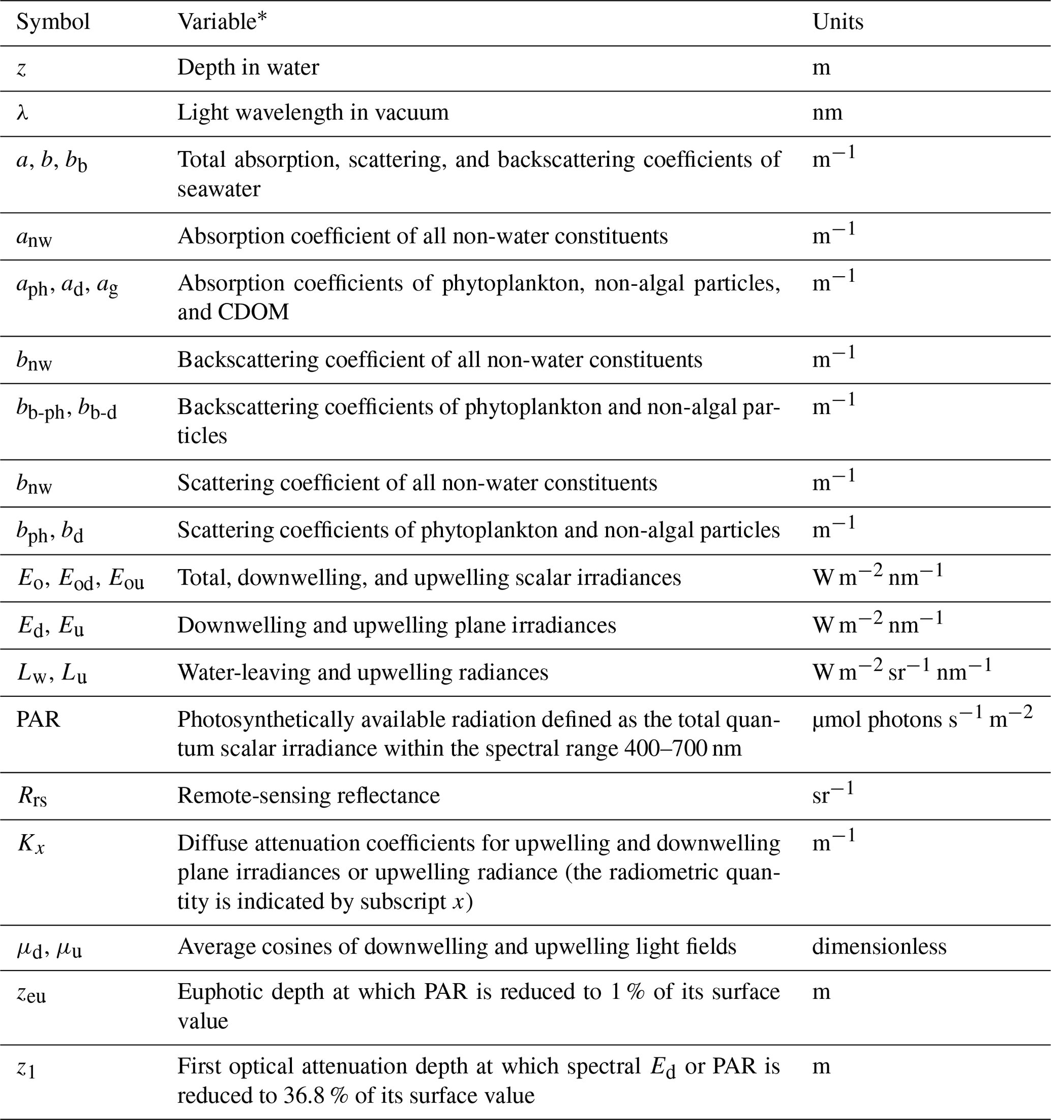
* All optical variables in the database are spectral and provided at different light wavelengths between 350 and 750 nm at 5 nm intervals and different depths within the water column between the sea surface and the 50 m depth, except for Rrs, and Lw, which are defined at the sea surface.
Figure 7 depicts scatter plots of IOP coefficients, specifically ag(440) vs. aph(440) (Fig. 7a), adg(440) vs. aph(440) (Fig. 7b), ad(440) vs. aph(440) (Fig. 7c), and bbp(550) vs. aph(440) (Fig. 7d). The scatter plots include two datasets, the in situ dataset and the synthetic dataset, as described in Sect. 2. We recall that in both types of datasets, aph(440) plotted on the x axis is the same because the phytoplankton absorption data used in this study were obtained from field measurements with no modeling involved. The scatter plots show a significant degree of overlap which indicates general consistency between the synthetic and in situ datasets. Similar patterns are observed when the , , , and ratios are plotted as a function of aph(440) (not shown). For illustrative purposes, the data from the synthetic IOP dataset are color coded to indicate the partitioning of data into the three OWGs, i.e., Groups 1, 2, and 3, which were defined using the synthetic spectra of Rrs(λ) generated through RT simulations with input of the synthetic IOP data. As expected, the data with the generally lowest values of IOPs belong to Group 3, the data with intermediate values of IOPs to Group 2, and the data with the highest IOPs (most turbid waters) to Group 1. We also note that the in situ dataset exhibits a somewhat wider dynamic range of variability than the synthetic dataset, especially when the IOP ratios, , , , and , are relatively high. While this result can reflect some degree of intrinsic difference in the dynamic range covered by the two datasets, it must also be recognized that some variability in the in situ dataset may be associated with the fact that these data were collected on numerous cruises by different groups of investigators using methodologies (instrumentation, data processing, data quality control, etc.) that are unavoidably different across the different data sources.
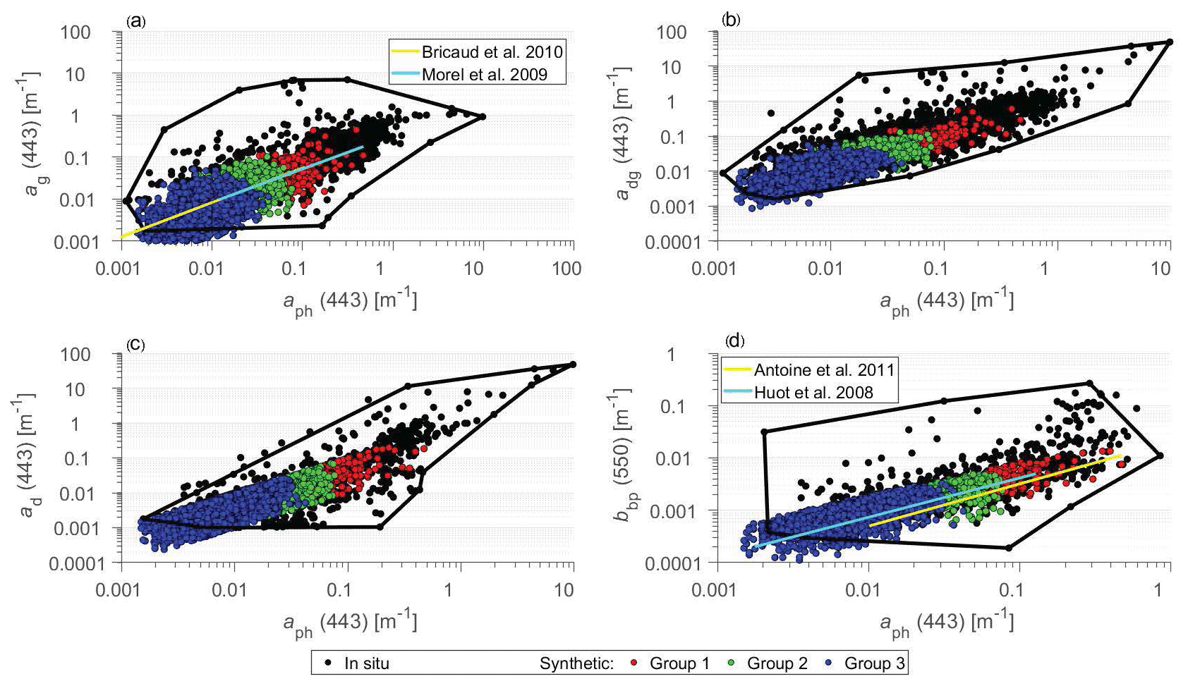
Figure 7(a) ag(443), (b) adg(443), (c) ad(443), and (d) bbp(550) as a function of aph(443) for the in situ dataset (black data points) and the synthetic dataset (colored data points). The black polygon lines in each panel delimit approximately the scatter of the in situ data points (black dots). Each color refers to the optical water group as indicated (139, 262, and 2919 data points for Group 1, 2, and 3, respectively). Empirical relationships previously developed for (a) ag(443) vs. aph(443) and (d) bbp(550) vs. aph(443) are also displayed for comparison. The original relationships were formulated as a function of Chla and the presented relationships were obtained by converting Chla to aph(443) using the chlorophyll-specific phytoplankton absorption at 443 nm from Bricaud et al. (1998).
For additional comparative purposes, Fig. 7a and d include a few empirical relationships between the IOPs in question, which were established in previous studies based on considerable amount of field measurements collected mostly in open-ocean environments. As seen, the relationships between ag(440) and aph(440) based on the studies of Morel (2009) and Bricaud et al. (2010) agree quite well with the central tendency of variation within our synthetic dataset. We note that Morel (2009) and Bricaud et al. (2010) reported relationships between ag(440) and Chla that were very similar in these studies. For the purpose of illustration in our Fig. 7a, we replaced Chla with aph(440) using the formula Chla =aph(440). Similarly, the studies of Huot et al. (2008) and Antoine et al. (2011) reported on empirical relationships between bbp(λ) and Chla. After converting Chla to aph(440) as mentioned above, these two relationship are plotted in Fig. 7d. Although these two relationships have different slopes, they are both generally consistent with the average trend of variation in the synthetic dataset.
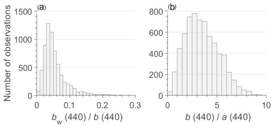
Radiative transfer is driven mainly by two ratios of IOPs, which are the scattering to absorption ratio, , which controls the number of scattering events (Morel and Gentili, 1991), and the molecular to total scattering ratio, , which is the parameter controlling the weighted sum of the particle scattering and molecular scattering phase functions (Morel and Loisel, 1998; Loisel and Stramski, 2000). Figure 8 shows the distribution of these two ratios at 440 nm for the synthetic dataset. The and ratios range between about 0 and 0.2 and between 0.5 and 10, respectively, which is consistent with previous models developed for Case 1 waters (Figs. 2 and 3 in Morel and Gentili, 1991; Fig. 2 in Morel and Loisel, 1998).
For comparing the AOPs from the synthetic database with in situ data, we have chosen two AOPs, the spectral remote-sensing reflectance, Rrs(λ), and the spectral diffuse attenuation coefficient of downwelling plane irradiance averaged within the water column from the sea surface to the first attenuation depth, 〈Kd(λ)〉1, as well as the maximum band ratio (MBR) of reflectance. The scatter plot of our synthetic data of Rrs(555) vs. Rrs(443) is depicted in Fig. 9a. For comparison, the range of in situ data is illustrated by the dashed contour lines. The maximum value of Rrs(443) reached 0.0165 sr−1, which is in good agreement with in situ measurements performed in ultra-oligotrophic waters in the South Pacific Gyre during the BIOSOPE cruise (see Fig. 3 in Stramski et al., 2008). These results are once again illustrated using color coding to represent different optical water types, specifically Groups 1, 2, and 3. As seen, there is relatively good agreement between the synthetic data and the range of variability of the in situ data for Groups 2 and 3 (Fig. 9a). For Group 1 (very turbid waters), however, the synthetic data exhibit a smaller range of variability compared with in situ data. This result is not unexpected because our primary goal was to generate the synthetic database that is most representative of open-ocean pelagic environments as well as coastal areas where water turbidity is low to moderate rather than very high. As described in Sect. 2, turbid waters of Group 1 correspond to OWCs 1 and 2 as defined in Mélin and Vantrepotte (2015). It is interesting to note that the synthetic optical database that was developed by Nechad et al. (2015) for coastal waters shows relatively good consistency between the synthetic and in situ data for Group 1 (Fig. 8b). However, in contrast to our synthetic database, the synthetic data of Nechad et al. (2015) exhibit a limited range of variability compared with in situ data for Groups 2 and 3. Thus, the synthetic data of Nechad et al. (2015) for turbid waters in Group 1 can provide useful complementarity to our synthetic database whose main focus is on water types from Groups 2 and 3.
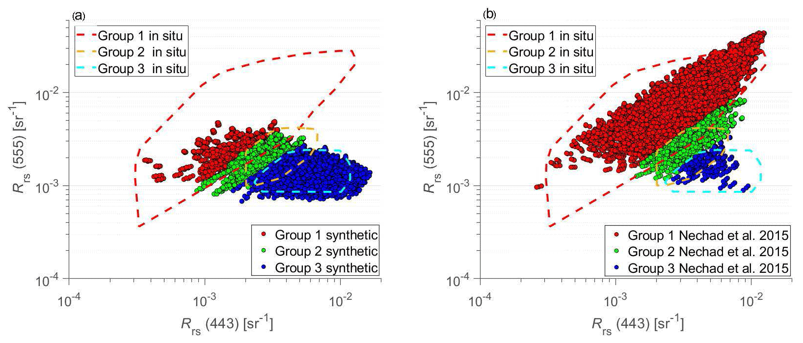
Figure 9(a) Rrs(555) as a function of Rrs(443) for the synthetic dataset (colored data points) and in situ dataset (colored contours). (b) Same as panel (a) but for the synthetic dataset of Nechad et al. (2015) that was developed for coastal waters. The color coding refers to the optical water groups as indicated.
The scatter plot of the synthetic data of 〈Kd(490)〉1 as a function of the blue-to-green band ratio of reflectance, , is shown in Fig. 10. These synthetic data are again color coded according to optical water classes defined in terms of Groups, 1, 2, and 3. For comparison, a few empirical relationships between these AOP variables established in previous analyses of field measurements are also displayed in Fig. 10 (Mueller, 2000; Werdell, 2005; Werdell, 2009). The relationship of Mueller (2000) was formulated during the early phase of the SeaWiFS satellite mission to serve as an operational global algorithm for estimating Kd(490) from ocean color observations. Werdell (2005) provided an updated relationship with a primary goal to improve the estimation of Kd(490) at low values of Kd(490) that correspond to high reflectance band ratio values. Figure 10 shows that these two relationships are generally consistent with our synthetic data across the entire range of variability encompassing data from Groups, 1, 2, and 3. This is reassuring given that the main purpose of our synthetic database and these two empirical relationships is similar in the sense of targeting the optical variability within the global ocean dominated by open-ocean environments. Figure 10 also includes the relationship of Werdell (2009) that represents the most recent update of global empirical algorithms for estimating Kd(490) from different ocean color satellite sensors. Specifically, the relationship of Werdell (2009) presented in Fig. 9 is referred to as KD2S and is based on SeaWiFS spectral bands. In contrast to the relationships of Mueller (2000) and Werdell (2005), the relationship of Werdell (2009) deviates significantly from our synthetic data within the range of relatively high values of 〈Kd(490)〉1, which correspond to relatively low values of . It is remarkable that this deviation occurs within the range where our synthetic data are classified as Group 1, so these optical water types are associated with high water turbidity. Another remarkable result illustrated in Fig. 10 is that the relationship of Werdell (2009) in this range is quite consistent with the main trend observed within the synthetic database of Nechad et al. (2015), which was developed for coastal environments. This result further supports the potential complementarity between our synthetic database and that of Nechad et al. (2015).
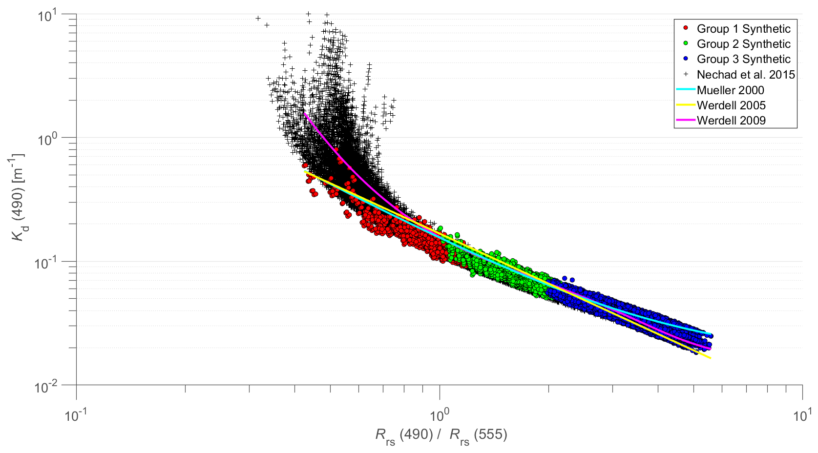
Figure 10Scatter plot of Kd(490) vs. the blue-to-green reflectance ratio, , for the synthetic database. The red, green, and blue data points represent OWGs 1, 2, and 3, respectively. The black cross data points are from the Nechad et al. (2015) synthetic dataset. The curves represent the relationships developed by Mueller (2000), Werdell (2005), and Werdell (2009). The Kd(490) data points represent 〈Kd(490)〉1 for the present synthetic database (colored data points) and the near-surface Kd(490) calculated within the top 1 cm layer for the Nechad dataset (black data points).
The scatter plot of Chla vs. the MBR of reflectance for the synthetic database is shown in Fig. 11. The monotonically decreasing trend of Chla with increasing MBR is consistent with the SeaWiFS-specific OC5 algorithm for estimating Chla from MBR (O'Reilly and Werdell, 2019). For this illustration, we estimated chl a using the relationship between aph(660) and Chla from Bricaud et al. (1998), which is unavoidably affected to some extent by natural variability in this relationship.
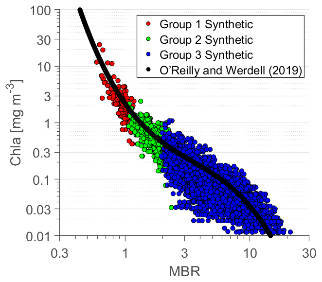
Figure 11Scatter plot of Chla vs. the blue-to-green maximum band ratio (MBR) of remote-sensing reflectance (i.e, ) for the synthetic database. The red, green, and blue data points represent OWG 1, 2, and 3, respectively. The solid black line represents the OC5 algorithm developed by O'Reilly and Werdell (2019) for SeaWiFS spectral bands. For this illustration, Chla was calculated from aph(660) using the chlorophyll-specific phytoplankton absorption at 660 nm from Bricaud et al. (1998).
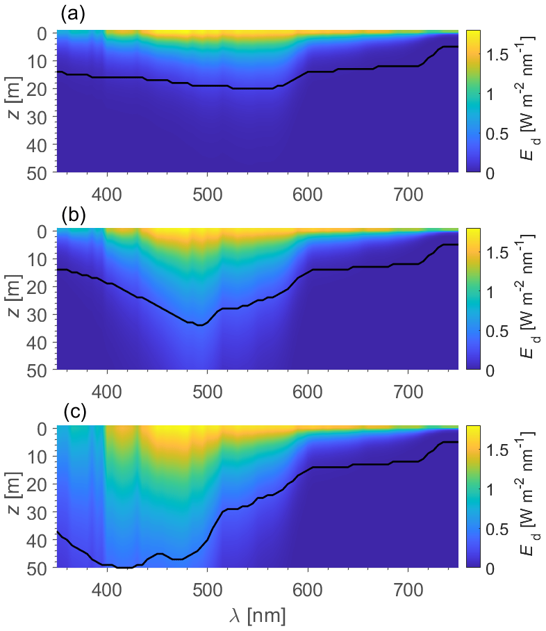
Figure 12Examples of depth profiles of Ed(z,λ) for a given IOP scenario from (a) OWG 1, (b) OWG 2, and (c) OWG 3. Radiative transfer simulations were performed for a sun zenith angle of 30∘ and included Raman scattering by water molecules and chlorophyll a fluorescence. The black line depicts the first optical attenuation depth, z1
The synthetic optical database described in this study is publicly available at the Dryad open-access repository of research data (Loisel et al., 2023; https://doi.org/10.6076/D1630T).
We have generated a new synthetic database that consists of seawater IOPs as well as corresponding radiometric quantities and AOPs within the ocean surface layer down to a depth of 50 m and at the sea surface. The radiometric quantities and AOPs were obtained from radiative transfer (RT) simulations performed with HydroLight code using the IOPs as input to the calculations. The list of variables included in the database is provided in Table 2. Because of the use of the absorption and scattering properties of pure seawater (assuming the salinity of 35 ‰) in the simulations, the present database cannot be applied to freshwater environments and special caution should be exercised for applications where water salinity is significantly less than 35 ‰ because of the decrease in pure seawater scattering. This database is organized following an easy-to-read NetCDF structure and divided into two subsets of data for which the file name identifies the sun zenith angle and the RT simulation scenario related to the presence or absence of inelastic radiative processes within the water column. The first subset of data includes the seawater spectral absorption and backscattering coefficients as well as sea-surface radiometric quantities relevant to ocean color radiometry, Rrs(λ), Lw(λ), , λ), and , λ), where is just above the surface. The surface and depth profile values of several spectral radiometric quantities and AOPs, as well as PAR, are included in the second subset of data. The spectra of zeu and z1 are also provided in the second file. More details on the organization and content of the database are included in the README file provided in the database.
In closing, we present an example illustration of one of the radiometric variables included in the output data files generated by RT simulations. We recall that the primary result of HydroLight simulations is the spectral radiance that provides comprehensive information about the angular distribution of the light field, from which different irradiances and AOPs are calculated. However, it is the spectral downwelling plane irradiance, Ed(z,λ), that has been the most commonly measured radiometric quantity in ocean optics, so in Fig. 12 we have chosen to illustrate HydroLight-simulated Ed(z,λ) within the ocean surface layer down to a depth of 50 m. These results are presented for three different scenarios of IOPs which are representative of three different optical water types defined in terms of Groups 1, 2, and 3 (see Sect. 2). These RT simulations were performed for the sun zenith angle of 30∘ in the presence of Raman scattering by water molecules and chlorophyll a fluorescence in the water column. In addition to significant differences in the variation of the spectral Ed(λ) as a function of depth z between Groups 1, 2, and 3, Fig. 12 also illustrates distinct differences in the magnitude and spectral behavior of the first optical attenuation depth, z1. This quantity is equivalent to the inverse of the diffuse attenuation coefficient, 〈Kd(λ)〉1. As expected, the first attenuation depth z1 is located much closer to the ocean surface for data from Group 1 (Fig. 12a) compared with Group 2 (Fig. 12b) and Group 3 (Fig. 12c), especially across the blue-to-green region of the spectrum. In the red part of the spectrum, where pure water absorption dominates the attenuation of Ed(λ), the differences between the three groups are small. It is also notable that the spectral behavior of z1 for Group 3 (Fig. 12c) that represents relatively clear ocean waters is remarkably similar to the spectral shape of the pure water absorption coefficient.
The concept of this study originated from the authors' discussions about the need for a new synthetic optical database in support of ocean color science and applications, especially global ocean applications, including support of NASA's upcoming PACE hyperspectral ocean color satellite mission. All co-authors contributed to the curation of the in situ data. HL and DSFJ led the generation of the synthetic IOP dataset and created the satellite IOP dataset. DSFJ ran the RT simulations. HL and DS wrote the article. All co-authors contributed to discussion, review, and editing of the article.
The contact author has declared that none of the authors has any competing interests.
Mention of trade names or commercial products does not
constitute endorsement or recommendation for use. The views expressed in
this article are those of the authors.
Publisher’s note: Copernicus Publications remains neutral with regard to jurisdictional claims in published maps and institutional affiliations.
We gratefully acknowledge all scientists and supporting personnel involved in the collection, processing, and dissemination of the in situ and satellite data used in this study as well as all agencies that provided support for these activities. We thank Jérôme Vialard for the generation of global SST data. We also thank Jaime Pitarch and two anonymous reviewers for comments on the manuscript.
This study was supported by the ANR CO2COAST project (grant no. ANR-20-CE01-0021 awarded to Hubert Loisel) and the National Aeronautics and Space Administration in the USA through the PACE project (NASA grant no. 80NSSC20M0252 awarded to Dariusz Stramski and Rick A. Reynolds).
This paper was edited by Salvatore Marullo and reviewed by Jaime Pitarch and two anonymous referees.
Antoine, D., Siegel, D. A., Kostadinov, T., Maritorena, S., Nelson, N. B., Gentili, B., Vellucci, V., and Guillocheau, N.: Variability in optical particle backscattering in contrasting bio-optical oceanic regimes, Limnol. Oceanogr., 56, 955–973, https://doi.org/10.4319/lo.2011.56.3.0955, 2011.
Aurin, D., Mannino, A., and Lary, D.: Remote sensing of CDOM, CDOM spectral slope, and dissolved organic carbon in the Global Ocean, Appl. Sci., 8, 2687, https://doi.org/10.3390/app8122687, 2018.
Babin, M., Stramski, D., Ferrari, G. M., Claustre, H., Bricaud, A., Obolensky, G., and Hoepffner, N.: Variations in the light absorption coe?cients of phytoplankton, nonalgal particles, and dissolved organic matter in coastal waters around Europe. J. Geophys. Res., 108, 3211, https://doi.org/10.1029/2001JC000882, 2003.
Bonelli, A. G., Vantrepotte, V., Jorge, D. S. F., Demaria, J., Jamet, C., Dessailly, D., Mangin, A., Fanton d'Andon, O., Kwiatkowska, E., and Loisel, H.: Colored dissolved organic matter absorption at global scale from ocean color radiometry observation: spatio-temporal variability and contribution to the absorption budget, Remote Sens. Environ., 265, 112637, https://doi.org/10.1016/j.rse.2021.112637, 2021.
Bricaud, A., Morel, A., Babin, M., Allali, K., and Claustre, H.: Variation of light absorption by suspended particles with chlorophyll a concentration in oceanic (case 1) waters: Analysis and implications for bio-optical models, J. Geophys. Res., 103, 31033–31044, https://doi.org/10.1029/98JC02712, 1998.
Bricaud, A., Babin, M., Claustre, H., Ras, J., and Tieche, F.: Light absorption properties and absorption budget of Southeast Pacific waters. J. Geophys. Res., 115, C0800910, https://doi.org/10.1029/2009JC005517, 2010.
Casey, K. A., Rousseaux, C. S., Gregg, W. W., Boss, E., Chase, A. P., Craig, S. E., Mouw, C. B., Reynolds, R. A., Stramski, D., Ackleson, S. G., Bricaud, A., Schaeffer, B., Lewis, M. R., and Maritorena, S.: A global compilation of in situ aquatic high spectral resolution inherent and apparent optical property data for remote sensing applications, Earth Syst. Sci. Data, 12, 1123–1139, https://doi.org/10.5194/essd-12-1123-2020, 2020.
Claustre, H., Sciandra, A., and Vaulot, D.: Introduction to the special section bio-optical and biogeochemical conditions in the South East Pacific in late 2004: the BIOSOPE program, Biogeosciences, 5, 679–691, https://doi.org/10.5194/bg-5-679-2008, 2008.
Craig, S. E., Lee, Z., and Du, K.: Top of Atmosphere, Hyperspectral Synthetic Dataset for PACE (Phytoplankton, Aerosol, and ocean Ecosystem) Ocean Color Algorithm Development, National Aeronautics and Space Administration, PANGAEA [data set], https://doi.org/10.1594/PANGAEA.915747, 2020.
Donlon, C., Berruti, B., Buongiorno, A., Ferreira, M.-H., Féménias, P., Frerick, J., Goryl, P., Klein, U., Laur, H., Mavrocordatos, C., Nieke, J., Rebhan, H., Seitz, B., Stroede, J., and Sciarra, R.: The Global Monitoring for Environment and Security (GMES) Sentinel-3 mission, Remote Sens. Environ., 120, 37–57, https://doi.org/10.1016/j.rse.2011.07.024, 2012.
Durack, P. J., Wijffels, S. E., and Boyer, T. P.: Long-term salinity changes and implications for the global water cycle, in: Ocean Circulation and Climate: A 21st Century Perspective, edited by: Siedler, G., Griffies, S. M., Gould, J., and Church, J. A., International Geophysics, vol. 103, Academic Press, Elsevier, Oxford, UK, 727–757, https://doi.org/10.1016/B978-0-12-391851-2.00028-3, 2013.
Fournier G. R. and Forand, J. L.: Analytic phase function for ocean water, in: Ocean Optics XII, edited by: Jaffe, J. S., Proc. SPIE, Vol. 2258, 194–201, https://doi.org/10.1117/12.190063, 1994.
Huot, Y., Morel, A., Twardowski, M. S., Stramski, D., and Reynolds, R. A.: Particle optical backscattering along a chlorophyll gradient in the upper layer of the eastern South Pacific Ocean, Biogeosciences, 5, 495–507, https://doi.org/10.5194/bg-5-495-2008, 2008.
IOCCG Report: Remote Sensing of Inherent Optical Properties: Fundamentals, Tests of Algorithms, and Applications, in: Reports of the International Ocean-Colour Coordinating Group (IOCCG), edited by: Lee, Z.-P. and Lee, Z.-P., No. 5, 126 pp., IOCCG, Dartmouth, NS, Canada, https://ioccg.org/wp-content/uploads/2015/10/ioccg-report-05.pdf (last access: 1 March 2023), 2006.
IOCCG Protocol Series: Inherent Optical Property Measurements and Protocols: Absorption Coefficient, in: IOCCG Ocean Optics and Biogeochemistry Protocols for Satellite Ocean Colour Sensor Validation, edited by: Neeley, A. R. and Mannino, A., vol. 1.0, 78 pp., IOCCG, Dartmouth, NS, Canada, https://doi.org/10.25607/OBP-119, 2018.
Jonasz, M. and Fournier, G. R.: Light Scattering by Particles in Water: Theoretical and Experimental Foundations, Academic Press, Amsterdam, ISBN-13: 978-0-12-388751-1, https://doi.org/10.1016/B978-0-12-388751-1.X5000-5, 2007.
Jorge, D. S. F., Loisel, H., Jamet, C., Dessailly, D., Demaria, J., Bricaud, A., Maritorena, S., Zhang, X., Antoine, D., Kutser, T., Bélanger, S., Brando, V. O., Werdell, J., Kwiatkowska, E., Mangin, A., and Fanton d'Andon, O.: A three-step semi analytical algorithm (3SAA) for estimating inherent optical properties over oceanic, coastal, and inland waters from remote sensing reflectance, Remote Sens. Environ., 263, 112537, https://doi.org/10.1016/j.rse.2021.112537, 2021.
Kishino, M., Takahashi, M., Okami, N., and Ichimura, S.: Estimation of the spectral absorption coefficient of phytoplankton in the sea, Bull. Mar. Sci., 37, 634–642, 1985.
Kostakis, I., Twardowski, M., Roesler, C., Röttgers, R., Stramski, D., McKee, D., Tonizzo, A., and Drapeau, S.: Hyperspectral optical absorption closure experiment in complex coastal waters, Limnol. Oceanogr. Methods, 19, 589–625, https://doi.org/10.1002/lom3.10447, 2021.
Kou, L., Labrie, D., and Chylek, P.: Refractive indices of water and ice in the 0.65 to 2.5 µm spectral range, Appl. Opt., 32, 3531–3540, https://doi.org/10.1364/AO.32.003531, 1993.
Lévy, M., Lehahn, Y., André, J.-M., L. Mémery, L., Loisel, H., and E. Heifetz, E.: Production regimes in the northeast Atlantic: A study based on Sea-viewing Wide Field-of-view Sensor (SeaWiFS) chlorophyll and ocean general circulation model mixed layer depth, J. Geophys. Res., 110, C07S10, https://doi.org/10.1029/2004JC002771, 2005.
Loisel, H. and Morel, A.: Light scattering and chlorophyll concentration in case 1 waters: a re-examination, Limnol. Oceanogr., 43, 847–857, 1998.
Loisel, H. and Stramski, D:. Estimation of the inherent optical properties of natural waters from irradiance attenuation coefficient and reflectance in the presence of Raman scattering, Appl. Opt., 39, 3001–3011, https://doi.org/10.1364/ao.39.003001, 2000.
Loisel, H., Nicolas, J.-M., Sciandra, A., Stramski, D., and Poteau, A.: Spectral dependency of optical backscattering by marine particles from satellite remote sensing of the global ocean, J. Geophys. Res.-Oceans, 111, C09024, https://doi.org/10.1029/2005JC003367, 2006.
Loisel, H., Mériaux, X., Berthon, J.-F., and Poteau, A.: Investigation of the optical backscattering to scattering ratio of marine particles in relation to their biogeochemical composition in the eastern English Channel and southern North Sea, Limnol. Oceanogr., 52, 739–752, https://doi.org/10.4319/lo.2007.52.2.0739, 2007.
Loisel, H., Mériaux, X., Poteau, A., Artigas, L. F., Lubac, B., Gardel, A., Caillaud, J., and Lesourd, S.: Analyze of the inherent optical properties of French Guiana coastal waters for remote sensing applications, J. Coast. Res., SI 56, 1532–1536, 2009.
Loisel, H., Vantrepotte, V., Norkvist, K., Mériaux, X., Kheireddine, M., Ras, J., Pujo-Pay, M., Combet, Y., Leblanc, K., Dall'Olmo, G., Mauriac, R., Dessailly, D., and Moutin, T.: Characterization of the bio-optical anomaly and diurnal variability of particulate matter, as seen from scattering and backscattering coefficients, in ultra-oligotrophic eddies of the Mediterranean Sea, Biogeosciences, 8, 3295–3317, https://doi.org/10.5194/bg-8-3295-2011, 2011.
Loisel, H., Stramski, D., Dessailly, D., Jamet, C., Li, L., and Reynolds, R. A.: An inverse model for estimating the optical absorption and backscattering coefficients of seawater from remote-sensing reflectance over a broad range of oceanic and coastal marine environments, J. Geophys. Res.-Oceans, 123, 2141–2171, https://doi.org/10.1002/2017JC013632, 2018.
Loisel, H., Jorge, D. S. F., Reynolds, R. A., and Stramski, D.: A synthetic database of hyperspectral ocean optical properties, Dryad [data set], https://doi.org/10.6076/D1630T, 2023.
Lubac, B., Loisel, H., Guiselin, N., Astoreca, R., Artigas, L. F., and Mériaux, X.: Hyperspectral versus multispectral remote sensing approach to detect phytoplankton blooms in coastal waters: Application to a Phaeocystis globosa bloom, J. Geophys. Res.-Oceans, 113, C06026, https://doi.org/10.1029/2007JC004451, 2008.
Maritorena, S., Morel, A., and Gentili, B.: Determination of the fluorescence quantum yield by oceanic phytoplankton in their natural habitat, Appl. Opt. 39, 6725–6737, https://doi.org/10.1364/AO.39.006725, 2000.
Maritorena, S., Siegel, D. A., and Peterson, A. R.: Optimization of a semianalytical ocean color model for global-scale applications, Appl. Opt., 41, 2705–2714, 2002.
Marshall, B. R. and Smith, R. C.: Raman scattering and in-water optical properties, Appl. Opt., 29, 71–84, https://doi.org/10.1364/AO.29.000071, 1990.
Mélin, F. and Vantrepotte, V.: How optically diverse is the coastal ocean?, Remote Sens. Environ., 160, 235–251, https://doi.org/10.1016/j.rse.2015.01.023, 2015.
Mobley, C.: A numerical model for the computation of radiance distributions in natural waters with wind-roughened surfaces, Limnol. Oceanogr., 34, 1473–1483, https://doi.org/10.4319/lo.1989.34.8.1473, 1989.
Mobley, C. D.: Light and Water. Radiative Transfer in Natural Waters, Academic Press, San Diego, ISBN 0-12-502750-8, 1994.
Mobley, C. D.: Hydrolight Technical Note 10: Interpretation of Raman Scattering Computations, Sequoia Scientific, Bellevue, WA, 2012.
Mobley, C. D. and Sundman, L. K.: HydroLight 5 EcoLight 5 Technical Documentation, Sequoia Scientific, Bellevue, WA, 2008.
Mobley, C. D., Gentili, B., Gordon, H. R., Jin, Z., Kattawar, G. W., Morel, A., Reinersman, P., Stamnes, K., and Stavn, R.: Comparison of numerical models for the computation of underwater light fields, Appl. Opt., 32, 7484–7504, https://doi.org/10.1364/AO.32.007484, 1993.
Morel, A.: Optical properties of pure water and pure seawater, in: Optical Aspects of Oceanography, edited by: Jerlov, N. G. and Steeman Nielsen, E., Academic Press, London, 1–24, ISBN-10: 0123849500, 1974.
Morel, A.: Are the empirical relationships describing the bio-optical properties of case 1 waters consistent and internally compatible?, J. Geophys. Res., 114, C01016, https://.org/10.1029/2008JC004803, 2009.
Morel, A. and Gentili, B.: Diffuse reflectance of oceanic waters: its dependence on Sun angles as influenced by the molecular scattering contribution, Appl. Opt., 30, 4427–4438, https://doi.org/10.1364/AO.30.004427, 1991.
Morel, A. and Loisel, H.: Apparent Optical properties of oceanic waters: dependence on molecular scattering contribution, Appl. Opt. 37, 4765–4776, https://doi.org/10.1364/ao.37.004765, 1998.
Morel, A. and Maritorena, S.: Bio-optical properties of oceanic waters: a reappraisal, J. Geophys. Res., 106, 7163–7180, https://doi.org/10.1029/2000JC000319, 2001.
Morel, A., Huot, Y., Gentili, B., Werdell, P. J., Hooker, S. B., and Franz, B. A.: Examining the consistency of products derived from various ocean color sensors in open ocean (Case 1) waters in the perspective of a multi-sensor approach, Remote Sens. Environ., 111, 69–88, https://doi.org/10.1016/j.rse.2007.03.012, 2007.
Morrison, J. R.: In situ determination of the quantum yield of phytoplankton chlorophyll a fluorescence: A simple algorithm, observations, and a model, Limnol. Oceanogr., 48, 618–631, https://doi.org/10.4319/lo.2003.48.2.0618, 2003.
Mueller, J. L.: SeaWiFS algorithm for the diffuse attenuation coefficient, K(490), using water-leaving radiances at 490 and 555 nm, in: SeaWiFS Postlaunch Calibration and Validation Analyses, Part 3, edited by: Hooker, S. B. and Firestone, E. R., NASA/TM-2000-206892, Vol. 11, NASA Goddard Space Flight Center, Greenbelt, Maryland, 24–27, 2000.
Nechad, B., Ruddick, K., Schroeder, T., Oubelkheir, K., Blondeau-Patissier, D., Cherukuru, N., Brando, V., Dekker, A., Clementson, L., Banks, A. C., Maritorena, S., Werdell, P. J., Sá, C., Brotas, V., Caballero de Frutos, I., Ahn, Y.-H., Salama, S., Tilstone, G., Martinez-Vicente, V., Foley, D., McKibben, M., Nahorniak, J., Peterson, T., Siliò-Calzada, A., Röttgers, R., Lee, Z., Peters, M., and Brockmann, C.: CoastColour Round Robin data sets: a database to evaluate the performance of algorithms for the retrieval of water quality parameters in coastal waters, Earth Syst. Sci. Data, 7, 319–348, https://doi.org/10.5194/essd-7-319-2015, 2015.
Neukermans, G., Loisel, H., Mériaux, X., Astoreca, R., and McKee, D.: In situ variability of mass-specific beam attenuation and backscattering of marine particles with respect to particle size, density, and composition, Limnol. Oceanogr., 57, 124–144, https://doi.org/10.4319/lo.2012.57.1.0124, 2012.
Neukermans, G., Reynolds, R. A., and Stramski, D.: Optical classification and characterization of marine particle assemblages within the western Arctic Ocean. Limnol. Oceanogr., 61, 1472–1494, https://doi.org/10.1002/lno.10316, 2016.
O'Reilly, J. E. and Werdell, P. J.: Chlorophyll algorithms for ocean color sensors – OC4, OC5 & OC6, Remote Sens. Environ., 229, 32–47, https://doi.org/10.1016/j.rse.2019.04.021, 2019.
Petzold, T. J: Volume scattering functions for selected natural waters, Scripps Inst. Oceanogr. Contrib. 72–78, San Diego, CA, 1972.
Pope, R. M. and Fry, E. S.: Absorption spectrum (380–700 nm) of pure water. II. Integrating cavity measurements, Appl. Opt., 36, 8710–8723, https://doi.org/10.1364/AO.36.008710, 1997.
Reynolds, R. A. and Stramski, D.: Optical characterization of marine phytoplankton assemblages within surface waters of the western Arctic Ocean, Limnol. Oceanogr., 64, 2478–2496, https://doi.org/10.1002/lno.11199, 2019.
Reynolds, R. A., Stramski, D., and Mitchell, B. G.: A chlorophyll-dependent semianalytical reflectance model derived from field measurements of absorption and backscattering coefficients within the Southern Ocean, J. Geophys. Res., 106, 7125–7138, https://doi.org/10.1029/1999JC000311, 2001.
Reynolds, R. A., Stramski, D., and Neukermans, G.: Optical backscattering of particles in Arctic seawater and relationships to particle mass concentration, size distribution, and bulk composition, Limnol. Oceanogr., 61, 1869–1890, https://doi.org/10.1002/lno.10341, 2016.
Stamnes, K., Thomas, G. E., and Stamnes, J. J.: Radiative Transfer in the Atmosphere and Ocean, 2nd edn., University Cambridge Press, Online ISBN 9781316148549, https://doi.org/10.1017/9781316148549, 2017.
Stavn, R. H.: Effects of Raman scattering across the visible spectrum in clear ocean water: A Monte Carlo study, Appl. Opt., 32, 6853–6863, https://doi.org/10.1364/AO.32.006853, 1993.
Stramski, D., Reynolds, R. A., Babin, M., Kaczmarek, S., Lewis, M. R., Röttgers, R., Sciandra, A., Stramska, M., Twardowski, M. S., Franz, B. A., and Claustre, H.: Relationships between the surface concentration of particulate organic carbon and optical properties in the eastern South Pacific and eastern Atlantic Oceans, Biogeosciences, 5, 171–201, https://doi.org/10.5194/bg-5-171-2008, 2008.
Stramski, D., Reynolds, R. A., Kaczmarek, S., Uitz, J., and Zheng, G.: Correction of pathlength amplification in the filter-pad technique for measurements of particulate absorption coefficient in the visible spectral region, Appl. Opt., 54, 6763–6782, https://doi.org/10.1364/AO.54.006763, 2015.
Stramski, D., Li, L., and Reynolds, R. A.: Model for separating the contributions of non-algal particles and colored dissolved organic matter to light absorption by seawater, Appl. Opt., 58, 3790–3806, https://doi.org/10.1364/AO.58.003790, 2019.
Stramski, D., Joshi, I., and Reynolds, R. A.: Ocean color algorithms to estimate the concentration of particulate organic carbon in surface waters of the global ocean in support of a long-term data record from multiple satellite missions, Remote Sens. Environ., 269, 112776, https://doi.org/10.1016/j.rse.2021.112776, 2022.
Sugihara, S., Kishino, M., and Okami, M.: Contribution of Raman scattering to upward irradiance in the sea, J. Oceanogr. Soc. Japan, 40, 397–404, 1984.
Uitz, J., Stramski, D., Reynolds, R. A., and Dubranna, J.: Assessing phytoplankton community composition from hyperspectral measurements of phytoplankton absorption coefficient and remote-sensing reflectance in open-ocean environments, Remote Sens. Environ., 171, 58–74, https://doi.org/10.1016/j.rse.2015.09.027.
Valente, A., Sathyendranath, S., Brotas, V., Groom, S., Grant, M., Taberner, M., Antoine, D., Arnone, R., Balch, W. M., Barker, K., Barlow, R., Bélanger, S., Berthon, J.-F., Beşiktepe, Ş., Borsheim, Y., Bracher, A., Brando, V., Canuti, E., Chavez, F., Cianca, A., Claustre, H., Clementson, L., Crout, R., Frouin, R., García-Soto, C., Gibb, S. W., Gould, R., Hooker, S. B., Kahru, M., Kampel, M., Klein, H., Kratzer, S., Kudela, R., Ledesma, J., Loisel, H., Matrai, P., McKee, D., Mitchell, B. G., Moisan, T., Muller-Karger, F., O'Dowd, L., Ondrusek, M., Platt, T., Poulton, A. J., Repecaud, M., Schroeder, T., Smyth, T., Smythe-Wright, D., Sosik, H. M., Twardowski, M., Vellucci, V., Voss, K., Werdell, J., Wernand, M., Wright, S., and Zibordi, G.: A compilation of global bio-optical in situ data for ocean-colour satellite applications – version two, Earth Syst. Sci. Data, 11, 1037–1068, https://doi.org/10.5194/essd-11-1037-2019, 2019.
Voss, K. J.: A spectral model of the beam attenuation coefficient in the ocean and coastal areas, Limnol. Oceanogr., 37, 501–509, 1992.
Werdell, P. J.: OceanColor K490 algorithm evaluation, NASA Ocean Color Web, https://oceancolor.gsfc.nasa.gov (last access: 1 March 2023), 2005.
Werdell, P. J.: Diffuse attenuation coefficient (KD) for downwelling irradiance at 490 nm, NASA Ocean Color Web, https://oceancolor.gsfc.nasa.gov (last access: 1 March 2023), 2009.
Werdell, P. J. and Bailey, S. W.: An improved in situ bio-optical data set for ocean color algorithm development and satellite data product validation, Remote Sens. Environ., 98, 122–140, https://doi.org/10.1016/j.rse.2005.07.001, 2005.
Westberry, T. K., Boss, E., and Lee, Z.-P.: Influence of Raman scattering on ocean color inversion models, Appl. Opt., 52, 5552–5561, https://doi.org/10.1364/AO.52.005552, 2013.
Whitmire, A. L., Pegau, W. S., Karp-Boss, L., Boss, E., and Cowles, T. J.: Spectral backscattering properties of marine phytoplankton cultures, Opt. Express, 18, 15073–15093, https://doi.org/10.1364/OE.18.015073, 2010.
Zhang, X. and Hu, L.: Estimating scattering of pure water from density fluctuation of the refractive index, Opt. Express, 17, 1671–1678, https://doi.org/10.1364/OE.17.001671, 2009.
Zhang, X., Hu, L., and He, M.-X.: Scattering by pure seawater: effect of salinity, Opt. Express, 17, 5698–5710, https://doi.org/10.1364/OE.17.012685, 2009.
Zhang, X., Huot, Y., Bricaud, A., and Sosik, H. M: Inversion of spectral absorption coefficients to infer phytoplankton size classes, chlorophyll concentration, and detrital matter, Appl. Opt., 54, 5805–5816, https://doi.org/10.1364/AO.54.005805, 2015.
Zheng, G., Stramski, D., and Reynolds, R. A.: Evaluation of the Quasi-Analytical Algorithm for estimating the inherent optical properties of seawater from ocean color: Comparison of Arctic and lower-latitude waters, Remote Sens. Environ., 155, 194–209, https://doi.org/10.1016/j.rse.2014.08.020, 2014.
- Abstract
- Introduction
- Development of a synthetic dataset of seawater inherent optical properties
- Radiative transfer simulations
- Comparisons of the synthetic database with in situ data
- Data availability
- Summary
- Author contributions
- Competing interests
- Disclaimer
- Acknowledgements
- Financial support
- Review statement
- References