the Creative Commons Attribution 4.0 License.
the Creative Commons Attribution 4.0 License.
 | 08 Aug 2023
The Coastal Surveillance Through Observation of Ocean Color (COASTℓOOC) dataset
Philippe Massicotte
Marcel Babin
Frank Fell
Vincent Fournier-Sicre
David Doxaran
Coastal Surveillance Through Observation of Ocean Color (COASTℓOOC) oceanographic expeditions were conducted in 1997 and 1998 to examine the relationship between the optical properties of seawater and related biological and chemical properties across the coastal to open-ocean gradient in various European seas. A total of 379 stations were visited along the coasts of the Gulf of Lion in the Mediterranean Sea (n=61), the Adriatic Sea (n=39), the Baltic Sea (n=57), the North Sea (n=99), the English Channel (n=85), and the Atlantic Ocean (n=38). Particular emphasis was placed on the collection of a comprehensive set of apparent and inherent optical properties (AOPs and IOPs) to support the development of ocean color remote-sensing algorithms. The data were collected in situ using traditional ship-based sampling but also from a helicopter, which is a very efficient means for that type of coastal sampling. The dataset collected during the COASTℓOOC campaigns is unique in that it is fully consistent in terms of operators, protocols, and instrumentation. This rich and historical dataset is still today frequently requested and used by other researchers. Therefore, we present the result of an effort to compile and standardize a dataset which will facilitate its reuse in future development and evaluation of new bio-optical models adapted for optically complex waters. The dataset is available at https://doi.org/10.17882/93570 (Massicotte et al., 2023).
- Article
(7198 KB) - Full-text XML
- BibTeX
- EndNote


Since the launch of the Coastal Zone Color Scanner (CZCS) by NASA in 1978, ocean color remote sensing has been used to monitor the state of and changes in global marine ecosystems in both time and space. In open oceans, the main component that affects the variations in the inherent and apparent optical properties (IOPs and AOPs) of seawater is phytoplankton, which is usually represented by the concentration of chlorophyll a (Morel and Prieur, 1977). Such open-ocean waters are traditionally termed Case-1 waters. Many simple spectral band-ratio algorithms have been developed to link changes in remotely sensed ocean color (OC), measured as reflectance, to variations in chlorophyll-a concentration (see O'Reilly and Werdell, 2019, for an extensive evaluation of OC band-ratio algorithms). Because these algorithms perform well, a plethora of studies have been conducted based on them, notably about phytoplankton phenology (e.g., Vargas et al., 2009) and phytoplankton primary production (see Carr et al., 2006, and references therein).
Spaceborne monitoring of aquatic ecosystems is more challenging for optically complex Case-2 waters (Morel and Prieur, 1977) often found in coastal areas. In contrast to Case-1 waters, the optical properties of Case-2 waters are determined by several types of constituents occurring in individually highly variable concentrations. Rivers draining large catchment areas deliver important quantities of optically significant substances such as chromophoric dissolved organic matter (CDOM) and suspended particulate matter (SPM) to coastal waters (Hedges et al., 1997; Cole et al., 2007; Massicotte et al., 2017). In shallow areas, bottom reflectance and resuspension of sediments can also alter the signal of water-leaving reflectance (Lee et al., 1998). Because CDOM and SPM do not necessarily co-vary with chlorophyll a and can mask the presence of phytoplankton (Sathyendranath, 2000), bio-optical algorithms developed for Case-1 waters are generally not appropriate for optically complex Case-2 waters (Gordon and Morel, 1983). Hence, concomitant in situ measurements of optically active components (CDOM, SPM, or chlorophyll a) and related radiometric quantities (AOPs and IOPs) are, to this day, critically needed to develop and improve bio-optical algorithms for coastal areas.
The objective of the Coastal Surveillance Through Observation of Ocean Color (COASTℓOOC) oceanographic expeditions was to acquire a comprehensive set of AOPs, IOPs, and concentrations of optically significant components along European coasts to help the development of new remote-sensing algorithms in optically complex waters. Back in 1997 and 1998, the COASTℓOOC campaigns were among the very first concerted efforts to fill the knowledge gaps in coastal marine optics by establishing a large, consistent, and comprehensive optical dataset for coastal waters. A total of 379 stations were visited along the coasts of the Mediterranean Sea, Adriatic Sea, Baltic Sea, North Sea, English Channel, and Atlantic Ocean, mostly in coastal but also open-ocean waters. While this unique set of data has been used or referenced over the years in numerous peer-reviewed publications (see the list in Appendix A), a reference final dataset, with well-documented quality controls, has never been published. Even though the COASTℓOOC campaigns were carried out more than 20 years ago, the rich and historical dataset that has been collected still has great potential to contribute to the development and evaluation of new bio-optical models adapted for optically complex waters. The goal of this paper is to formally present a quality-controlled and final reference version of the COASTℓOOC dataset archived in a public repository where users can download it readily.
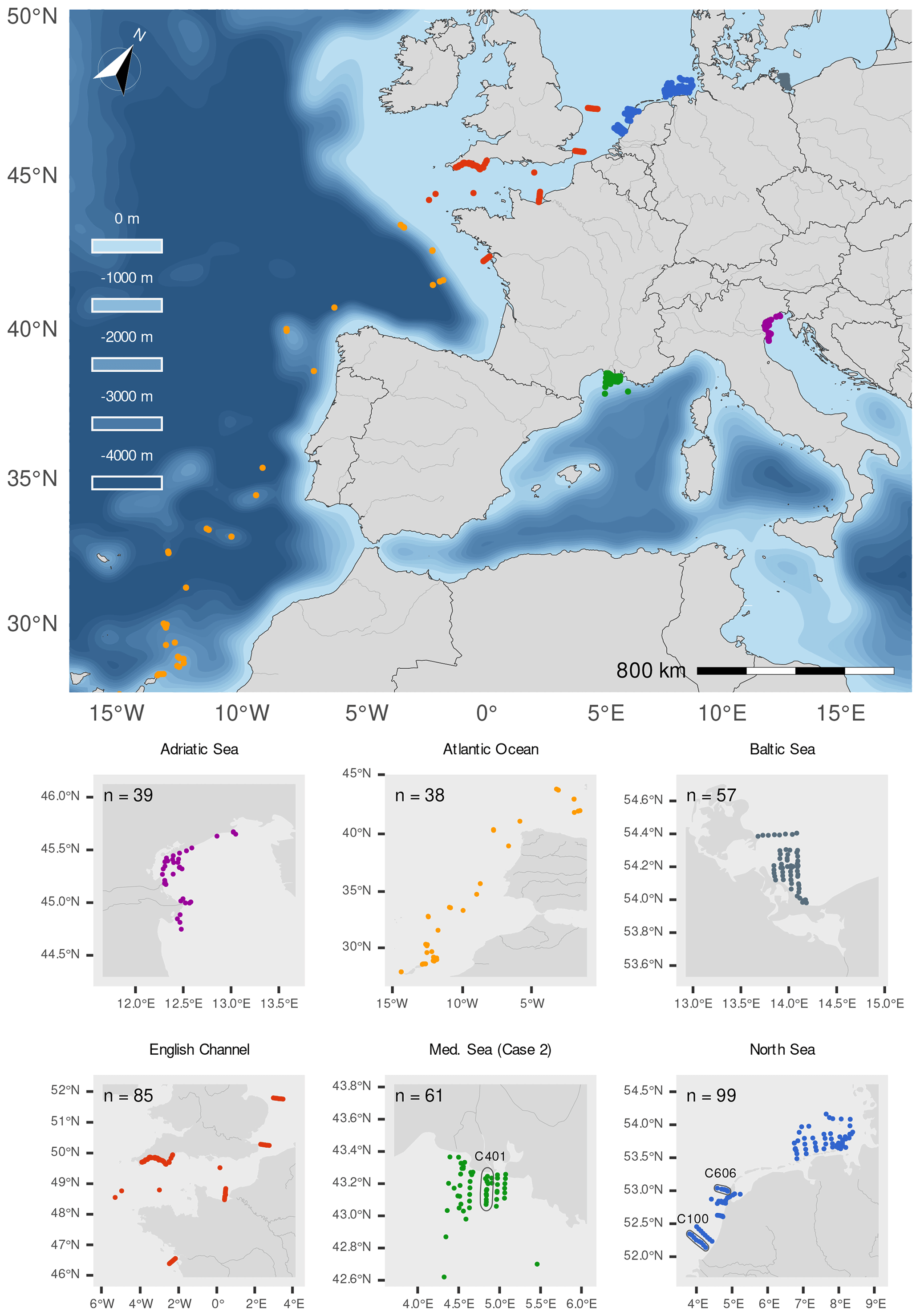
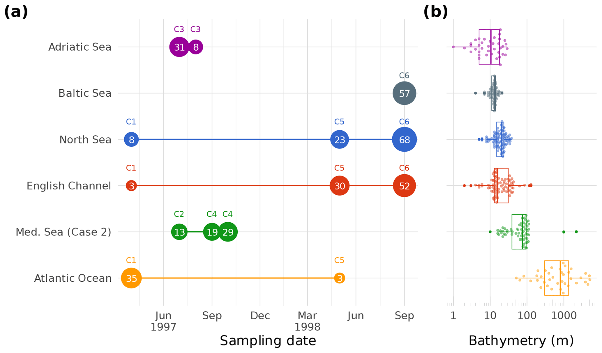
Figure 2(a) Overview of the temporal sampling for the six areas. The numbers in the circles indicate the number of visited stations each month. (b) Boxplot showing the bathymetry at the sampling locations by area. The labels on top of each circle identify the COASTℓOOC campaigns (C1 to C6).
2.1 Study area and general sampling strategy
During the six COASTℓOOC campaigns, further referred to as C1 to C6, a total of 379 locations were visited (Fig. 1). The stations were located along the coasts of the Gulf of Lion in the Mediterranean Sea (n=61), the Adriatic Sea (n=39), the Baltic Sea (n=57), the North Sea (n=99), the English Channel (n=85), and the Atlantic Ocean (n=38). Within each area, the stations were generally distributed along across-shore or along-shore transects to capture the land-to-sea gradients and document river plumes (Fig. 1b). COASTℓOOC campaigns were either ship-based (C1, C4, C5) or used a helicopter as a sampling platform (C2, C3, C6) and took place between 2 April 1997 and 25 September 1998 (Fig. 2a). Compared to traditional ship-based sampling, the helicopter platform allowed efficient stations close to the coast in areas difficult to access by boat (some samples were collected in waters as shallow as 1 m, Babin, 2003). Combining both ship and airborne sampling approaches allowed the whole inshore to open-ocean aquatic continuum to be covered. The bathymetry (GEBCO Bathymetric Compilation Group 2021, 2021) varied greatly across the stations, where it averaged ca. 10 m in the Adriatic Sea and ca. 800 m in the Case-1 Atlantic Ocean (Fig. 2b).
2.2 Water sampling and processing
On board the ship, water samples were analyzed and/or stored immediately after collection. When using a helicopter as a sampling platform, water samples were kept in polyethylene containers for no longer than 2 h after sampling (see Babin, 2003, for further details). Filtration was conducted at low vacuum onto 25 mm glass-fiber filters (Whatman, GF/F) to collect particles for subsequent analyses as described below. Three separate subsamples (up to 2 L each) were filtered for each sample with the following purposes. To determine the concentration of SPM (g m−3), the particles collected onto a pre-weighed GF/F filter were dried and stored in a freezer at −80 ∘C until the dry weight was determined less than 2 months later in the laboratory (Van Der Linde, 1998). For pigment analysis, the filter with collected particles was inserted into a cryotube and kept in liquid nitrogen until analysis less than 3 months later. High-performance liquid chromatography (HPLC) was used as described by Vidussi et al. (1996) to determine liposoluble pigment concentrations. Total chlorophyll a is defined here as the sum of chlorophyll a, divinyl chlorophyll a, chlorophyll-a isomer and epimer, chlorophyllids a, and pheopigments. The concentrations of particulate organic carbon and nitrogen (POC and PON, respectively) were determined using a Carlo Erba NCS 2500 elemental analyzer as described in Ferrari et al. (2003). These determinations were made on particles collected on a GF/F filter precombusted at 450 ∘C for 2 h and stored in the freezer at −80 ∘C until analysis less than 2 months later. Further details concerning laboratory analyses can be found in Babin (2003), Ferrari (2000), and Ferrari et al. (2003). To determine the concentration of dissolved organic carbon (DOC, M), seawater samples were filtered on a 0.22 mm Millipore membrane. The final filtrate was transferred to a 100 mL amber-glass bottle, stored in the refrigerator, and analyzed within 3 weeks. DOC was determined by high-temperature catalytic oxidation using a Carlo Erba 480 analyzer. The methodological details can be found in Ferrari (2000).
2.3 Optical measurements
At each station, an optical package was deployed in the water column from the surface, down to 1 to 2 m above the ocean bottom in shallow waters, and to maximum depths of ca. 100 m in deep waters. The package included CTD (conductivity, temperature, and depth) and an array of optical instruments to simultaneously measure beam attenuation, absorption and scattering coefficients, as well as irradiance in the water column. The Modular Data and Power System (MODAPS) data-gathering system from Wetlabs Inc., USA, was used to combine the time-stamped data from the different instruments to produce a data matrix with a common depth grid. For further information, please refer to the COASTℓOOC final report (Aiken et al., 2000).
A specific aspect of COASTℓOOC is the use of a helicopter as a sampling platform, which has enabled high-frequency visiting of sites in very shallow waters (see Sect. 2.1). An additional advantage is the fact that helicopter-based optical measurements are not influenced by the sampling platform itself, unlike ship-based measurements unavoidably affected by the presence of the ship's hull, most prominently close to the surface. A drawback of this approach is the difficulty in operating a helicopter stationary at a constant height, especially under low or gusty wind conditions: while the former requires substantial flight heights to prevent the helicopter downdraft from impacting the optical measurements, rendering sampling less efficient, the latter can result in unwanted vertical movements of the instrument package in water on the order of 1–2 m s−1. To ensure the availability of data of sufficient quality close to the surface, several consecutive upcasts and downcasts were therefore performed at each “helicopter” site. Among the measured vertical profiles at each site, the most suitable casts for depth merging and surface extrapolation (which are not necessarily the same; see the end of Sect. 2.3.3) were selected using a combination of objective criteria and visual inspection.
2.3.1 Irradiance measurements
The SeaWiFS Profiling Multichannel Radiometer (SPMR, Satlantic Inc., Canada) was used to measure downward (Ed) and upward (Eu) spectral irradiances () in the water column. Irradiance was measured at 13 wavelengths matching the MEdium Resolution Imaging Spectrometer (MERIS) channels of direct relevance for ocean observations (411, 443, 456, 490, 509, 531, 559, 619, 664, 683, 706, 779, and 866 nm, except for COASTℓOOC 1 operating at 590 nm instead of 619 nm), ranging from the blue part of the spectrum to the near-infrared at an acquisition rate of 6 Hz. The actual wavelengths differ slightly between upward and downward observations.
The SPMR was fixed to the IOP instrument frame, except for the COASTℓOOC 5 mission, where it was used in free-falling mode. For the ship-based measurements, concomitant observations of the in-air downward spectral irradiance at the sea surface were performed to account for changes in the incoming solar radiation during the in situ profiling (e.g., due to clouds). This approach was not achievable for the helicopter-based measurements, since there was no suitable place to mount the radiometer. For these campaigns, measurements of Ed made by the profiler while in the air (i.e., before and after the in-water measurements) were used to assess Ed on the sea surface. In order to minimize the time lag between the in-water measurements and the Ed values on the sea surface, our processing code automatically chose the air measurements closest in time. Under stable atmospheric conditions, no significant error is expected to result from this approach, while it will contribute to increased variability in the retrieved parameters when sampling under varying cloud cover. However, the practical impact of this is limited due to the short duration of helicopter-based sampling, typically lasting between 1 and 3 min per profile.
2.3.2 Water-leaving reflectance
To calculate the water-leaving reflectance, accurate measurements of both Ed and Eu just below the water surface () are needed. In case no spectrally matching in-air Ed reference data are available (as is the case for the helicopter-based campaigns), this was done by extrapolating both Ed(z) and Eu(z) vertical profiles toward the sea surface by fitting an exponential model for the depth dependence of the measured spectral irradiance values (Eq. 1):
where Γ(λ,z) is either Ed or Eu measured at wavelength λ and at depth z, is Ed or Eu estimated just below the air–water interface, and KΓ is the estimated diffuse attenuation coefficient for downward (, m−1) or upward (, m−1) irradiance. Note that a correction to account for instrument self-shading of the upwelling irradiance was not applied. We assume that the impact of this omission is relatively small except for highly absorbing waters (depending on constituent concentration and/or observation wavelength), where it may lead to an underestimation of near-surface upwelling irradiances.
In case concomitant spectrally matching in-air Ed (0+) reference data are available (as is the case for most ship-based campaigns), Ed (0−) is calculated from Ed (0+) by applying a constant factor of 0.943 to account for losses of the downwelling irradiance (direct + diffuse) due to Fresnel reflection at the rough sea surface. The derived Eu (0−) and Ed (0−) values were thereafter used to calculate the water reflectance R (0+) just below the sea surface:
Vertical irradiance profiles in the red and near-infrared channels at wavelengths beyond 600 nm were fitted using a sum of two exponential functions, of which one represents the diffuse attenuation due to absorption and elastic scattering for the channel under consideration, while the other accounts for Raman scattering from the corresponding (shorter) excitation wavelengths significantly contributing to the upward light field (e.g., Sugihara et al., 1984). Not doing so, i.e., using just a single exponential function, leads to substantial underestimation of the extrapolated subsurface values due to significant Raman contributions from excitation wavelengths with significantly lower K values (see Appendix A). Figure A1 showing the near-surface depth dependence of Eu at 779 nm demonstrates why the two-function approach is required. Below a depth of ca. 1.5 m, the signal is strongly dominated by Raman scattering and is therefore characterized by a diffuse attenuation coefficient very close to that of the corresponding excitation wavelengths.
2.3.3 Irradiance depth merging
Depth-merged irradiance profiles were derived for all the sites by applying a standardized approach. The underlying strategy for depth merging was to provide users with the information they need to do their analyses while modifying the original data as little as possible. Processing was therefore limited to procedures that could be applied equally to all COASTℓOOC campaigns, whether helicopter- or ship-based. For example, variations of the incoming solar radiation were not considered in the depth-merging process, since such observations were not available for the helicopter-based campaigns. However, if measured while operating from research vessels, such information is included in the depth-merged profile data to allow users to do their own subsequent analyses.
Typically, several upcast and downcast vertical profiles were performed, especially when using the helicopter as a sampling platform, to increase the potential availability of high-quality observations. The actual merging process was executed as follows. First, any observation not meeting both of the following two conditions was discarded: (1) SPMR instrument tilt smaller than 20∘; (2) SPMR vertical speed between 0.1 and 2.0 m s−1. To automatically identify the best-suited cast for profile generation, the observations fulfilling the above two conditions were then distributed cast-wise over 0.2 m wide vertical bins, starting at zero depth. Finally, the cast with the highest number of bins containing at least one valid observation was selected for depth profile generation if it fulfilled two further conditions: (3) at least 2 m vertical distance between the highest and lowest bins and (4) at least 50 % of the bins containing at least one observation. No depth-merged data are provided for stations where there is no cast fulfilling all of the above four conditions. Combining several casts taken at one station has not proven successful due to potentially large discontinuities in the aggregated values at depth levels where the number of available casts changes, especially under unstable atmospheric conditions with the corresponding short-term irradiance fluctuations.
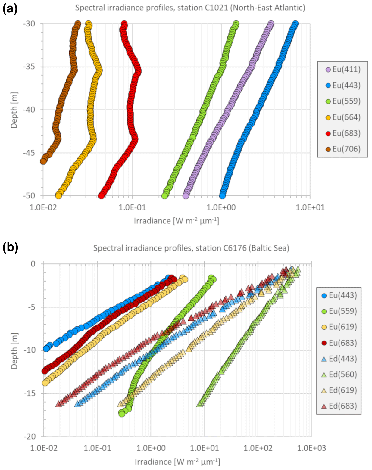
Figure 3(a) Vertical profile of the upwelling irradiance taken on 11 April 1997 at station C1021 located in the northeastern Atlantic offshore of northern Portugal. (b) Vertical profiles of the upwelling and downwelling irradiances taken on 25 September 1998 at station C6176 located in the Baltic Sea offshore of Usedom in northeastern Germany. See the text for further details.
Actual depth merging was done by taking the median of all the observations of a particular irradiance parameter within each depth bin. Spectral irradiance observations were only considered for values above 0.01 to reduce the impact of residual dark-current and radiometric noise. Finally, an attempt was made to identify and mask out remaining outliers in the depth-merged irradiance profiles. This was done by applying Grubb's test at a 5 % significance level (Guthrie, 2012) to the residual of a second-order polynomial fit of the logarithmic-transformed spectral irradiance observations for a 2 m deep window sliding down in steps of 1 m. While this procedure has successfully identified individual spikes, some obvious outliers extending over several depth bins remain in the merged dataset, and users will need to make their own judgment on how to identify and remove those.
Examples of depth-merged irradiance profiles are shown in Fig. 3 for one clear-water site in the northeastern Atlantic (Fig. 3a) and one CDOM-rich site in the Baltic Sea (Fig. 3b). Figure 3a features a double deep chlorophyll maximum with the corresponding irradiance increase due to chlorophyll fluorescence at water depths between ca. 35 and 45 m, most prominently visible at 683 nm but also affecting the neighboring channels at 664 and 706 nm. Diffuse attenuation in the blue to green wavelengths is correspondingly enhanced, as reflected by the change in slope at a depth of ca. 34 m. Figure 3b features Baltic Sea waters rich in CDOM, resulting in strong absorption in the UV and blue parts of the spectrum. The reduced decrease in the upwelling irradiance at 559 nm toward larger depths is likely caused by the reflection of downwelling irradiance from the ocean bottom, while chlorophyll fluorescence is likely the reason for the relatively enhanced (change in slope) upwelling irradiance at 683 nm for depths below ca. 7 m.
Note that extrapolated surface values and depth-merged profiles for a specific site are not necessarily derived from the same observations. This is especially true for helicopter-based operations typically comprising several upcasts and downcasts close to the water surface to increase the likelihood of having sufficient observations for the surface extrapolation, while usually only one or two deep-water casts were made to obtain observations at greater depth. The best-suited observations for surface extrapolation, therefore, do not necessarily correspond to the cast used for depth merging.
2.3.4 Profiles of the diffuse attenuation coefficient
Downward (, m−1) and upward (, m−1) spectral diffuse attenuation coefficients have been derived from the depth-merged irradiance data by fitting an exponential function through the irradiance observations within a 2 m deep window, sliding down in steps of 0.2 m. The calculation was only performed if at least five observations were available for fitting within the depth window. The choice of window width was based on a compromise between two conflicting requirements. On the one hand, it should be small enough to allow resolution of relatively narrow vertical features, such as a deep chlorophyll maximum. On the other hand, it should be large enough to allow for an accurate estimation of K. The window width of 2 m chosen herein favors vertical resolution over accuracy: while even relatively narrow vertical features remain distinguishable in their own derived K profiles, these are on the other hand affected by remaining outliers, instrument tilt variations, or instrumental noise. Obviously, users may use depth-merged irradiance profiles to derive K profiles or depth-integrated K values that better meet individual requirements.
2.3.5 Chromophoric dissolved organic matter (laboratory measurements)
Measurements of CDOM absorption (aCDOM, m−1) were performed in the laboratory using a spectrophotometer (Perkin Elmer, Lambda 12) on water samples (10 cm cuvette path length) filtered on a 0.22 µm Millipore membrane pre-rinsed with 50 mL of Milli-Q water (Babin, 2003). aCDOM spectra were measured between either 300–750 or 350–750 nm at a 1 nm increment.
2.3.6 Particulate, non-algal, and phytoplankton absorption (laboratory measurements)
Water samples were filtered onto 25 mm glass-fiber filters (Whatman, GF/F) at a low vacuum before absorption measurement (Babin, 2003). Total particulate absorption (aP, m−1) was measured on particles retained on the filters between 380 and 750 nm at a 1 nm increment using a spectrophotometer equipped with a 60 mm integrating sphere (Perkin Elmer, Lambda 19) and following the transmittance–reflectance (TR) method (Tassan and Ferrari, 1995, 1998). Afterward, pigments were removed from the particles with sodium hypochlorite to measure non-algal (or non-pigmented) absorption (aNAP, m−1). Finally, phytoplankton absorption (aϕ, m−1) was retrieved by subtracting aNAP from aP. aCDOM and aNAP absorption spectra were fitted according to the following equation (Jerlov, 1968; Bricaud et al., 1981):
where aτ is the absorption coefficient, either aCDOM or aNAP (m−1), λ is the wavelength (nm), λ0 is a reference wavelength (443 nm), Sτ is the spectral slope (nm−1) that describes the approximate exponential decrease in absorption with increasing wavelength, and k is a background constant (m−1) accounting for scatter in the cuvette and drift of the instrument. aCDOM spectra were fitted using observations below 700 nm, whereas aNAP fits were performed between 380 and 730 nm, excluding spectral regions between 400–480 and 620–710 nm to avoid possible residual pigment absorption (Babin, 2003). aCDOM and aNAP were baseline-corrected by subtracting the background parameter (k) derived from the following equation:
Finally, the spectral background of aP spectra (i.e., the average absorption measured between 746 and 750 nm) was added to aNAP. The underlying rationale is that absorption by phytoplankton in the near-infrared (NIR) is null and that absorption measured in the NIR for total particles using the TR method is real (Tassan and Ferrari, 2003) and belongs exclusively to non-algal particles. The absorption signal measured for total particles retained on untreated filters is assumed to be more reliable than that measurement on bleached filters.
2.3.7 Total absorption and scattering (in situ measurements)
In situ vertical profiles of absorption (a, m−1) and beam attenuation (c, m−1) were acquired at nine wavelengths (412, 440, 488, 510, 555, 630, 532 or 650 depending on the instrument configuration, 676, and 715 nm) using a flow-through in situ absorbance–attenuance meter (AC9, Wetlabs). As the measurements are referenced to pure (Milli-Q) water, the obtained absorption and attenuation coefficients exclude the contribution of water. To correct absorption measurements for incomplete recovery of scattered light, a(715) was subtracted from a(λ≤715). Scattering coefficients (b, m−1) were calculated by subtracting absorption from attenuation. As the contribution of molecular (water) scattering is excluded (see above), this coefficient essentially corresponds to particle scattering and is hereafter denoted by bp (m−1).
The derived values for a, bp, and c derived in this way were subsequently averaged over the first attenuation length () to provide values representative of the surface layer. Due to practical difficulties when operating the AC9 from a helicopter (e.g., trapped air in the instrument), the availability of a, bp, and c values is limited for helicopter-based campaigns, especially for COASTℓOOC 3 (Adriatic Sea). Surface-to-bottom depth merging of the full AC9 profiles has not been attempted so far, but this is envisaged for potential future reprocessing of the COASTℓOOC dataset (see Sect. 5).
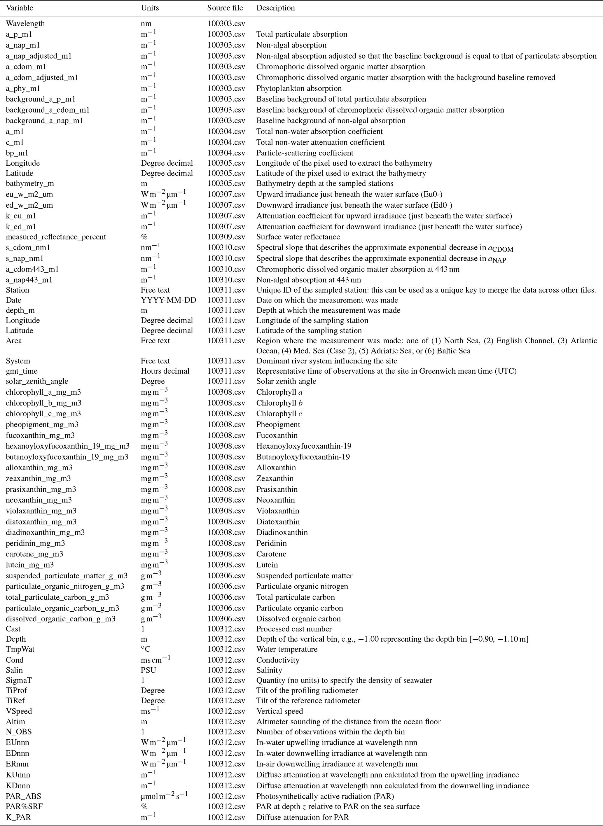
Different general quality-control procedures were adopted to ensure the integrity of the data. First, the raw data were visualized and screened to eliminate both errors originating from the measurement devices, including sensors (systematic or random), and errors inherent to measurement procedures and methods. Statistical metrics such as average, standard deviation, and range were computed to detect and remove anomalous values in the data. Then, data were checked for duplicates and remaining outliers. The complete list of variables is presented in Table 1.
4.1 Spatial variability along the coastal–ocean gradient
The COASTℓOOC sampling strategy was primarily designed to capture the bio-optical gradient across the sampled ecosystems and along transects from the coast toward the open ocean within each area (Fig. 1). The following sections present an overview of a few selected variables measured in the different areas. An extensive and detailed explanatory visualization analysis is presented in the final report of the COASTℓOOC project (Aiken et al., 2000).
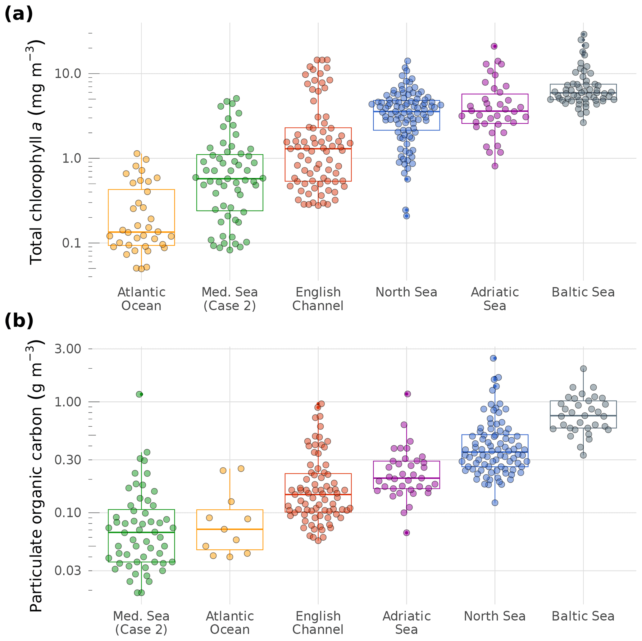
Figure 4(a) Total chlorophyll a and (b) particulate organic carbon across the sampled areas.
4.1.1 Chlorophyll a and particulate organic carbon
As observed in Fig. 4, both total chlorophyll-a and POC concentrations varied markedly across the sampled areas, reflecting the natural gradient captured by the sampling strategy. Across all the stations, total chlorophyll a ranged between 0.05 and 29 mg m−3. The median chlorophyll a ranged between ca. 0.15 mg m−3 in the Atlantic Ocean and 5.9 mg m−3 in the Baltic Sea (Fig. 4a). Based on the definition proposed by Antoine et al. (1996), the sampled stations were representative of a wide range of trophic statuses: oligotrophic (n=17, chlorophyll a ≤ 0.1 mg m−3), mesotrophic (n=106, 0.1 ≤ chlorophyll a ≤ 1 mg m−3), and eutrophic (n=245, chlorophyll a > 1 mg m−3). A similar shore-to-sea gradient pattern could be observed for POC, with median values varying between ca. 0.07 g m−3 and 0.8 g m−3 in the Mediterranean Sea (Case 2) and the Baltic Sea, respectively (Fig. 4b, range between 0.02 and 2.5 g m−3).
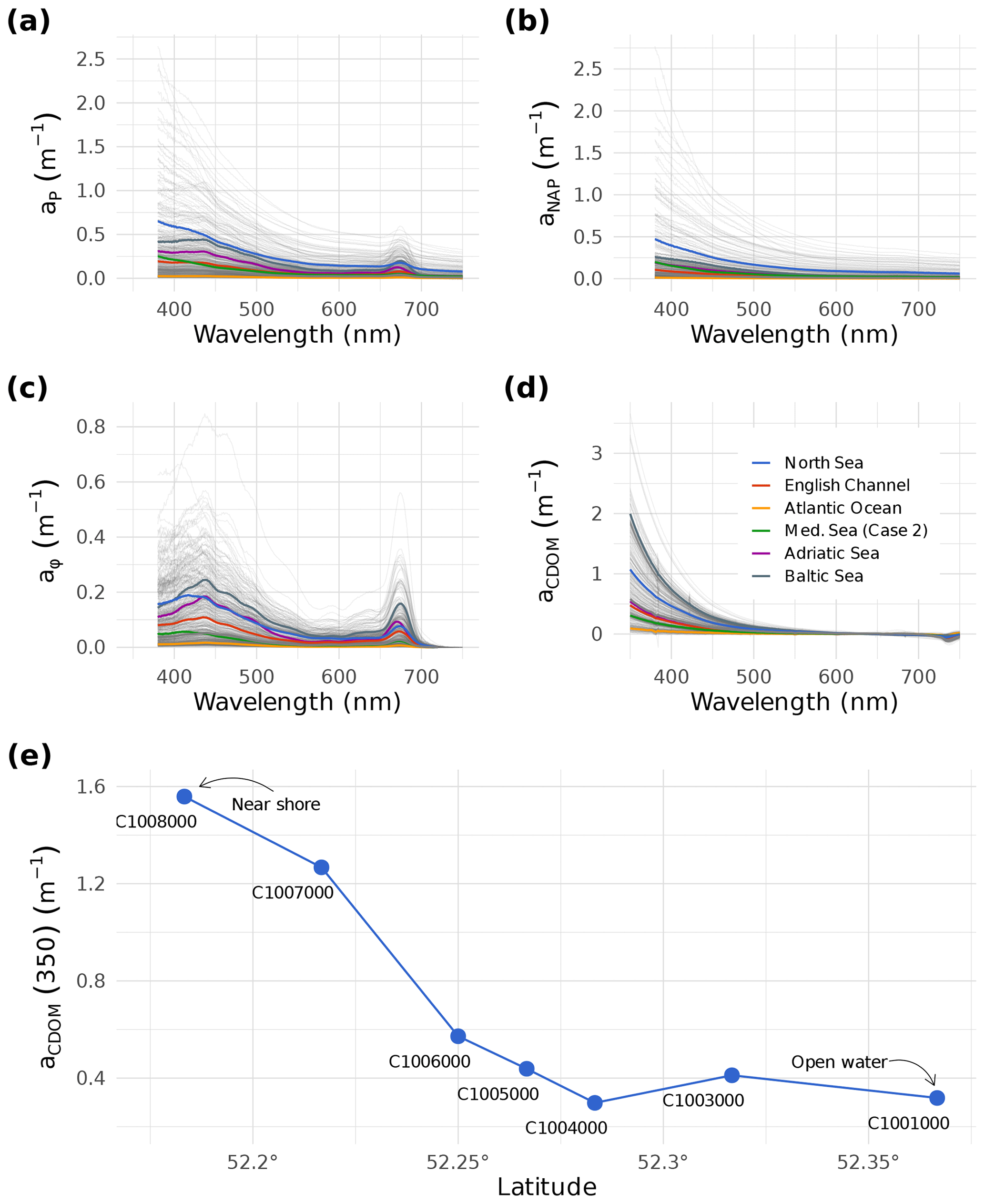
Figure 5(a) Average total particulate (ap), (b) non-algal (aNAP), (c) phytoplankton (aϕ), and (d) chromophoric dissolved organic matter (aCDOM) absorption spectra in each area. Light gray lines in panels (a–d) show individual absorption spectra measured across the sampled areas. (e) aCDOM(350) along the westernmost transect in the North Sea (see Fig. 1b).
4.1.2 IOPs
Measured absorption spectra in each area for total particulates (aP), non-algal particles (aNAP), phytoplankton (aϕ), and chromophoric dissolved organic matter (aCDOM) are presented in Fig. 5. Phytoplankton maximum absorption peaks at around 440 and 675 nm are easily distinguishable in Fig. 5c and were found to be highly correlated with the concentration of total chlorophyll a (Pearson's r > 0.90). Across all the areas, aCDOM(350), a proxy for dissolved carbon concentration, varied between 0.03 and 3.66 m−1. These values fall within the ranges of the mean values reported globally in the ocean (0.14 m−1), coastal (1.82 m−1), and estuarine (4.11 m−1) ecosystems (Massicotte et al., 2017). Overall, the highest absorption by dissolved organic matter was observed in the Baltic Sea (Fig. 5d). Sampled stations in this area were located west of the Oder River plume, which drains important quantities of humic substance from its catchment area. In contrast, the lowest CDOM absorption was observed in the Atlantic Ocean, where stations were located away from land and thus less influenced by terrestrial inputs (Fig. 1). The spatial variability of CDOM is further emphasized in Fig. 5e, where aCDOM(350) decreased by a factor of 4 between the two most distant points (approximately 40 km) of the westernmost transect sampled in the North Sea (see Fig. 1b).
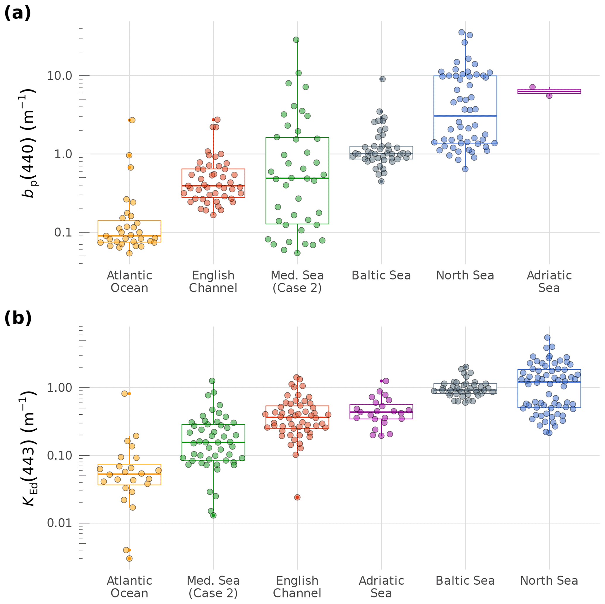
Figure 6(a) Particulate scattering coefficient at 440 nm (bb(440)) and (b) attenuation coefficient for downward irradiance at 443 nm (KEd(443)) across the sampled areas.
Light scattering by suspended particles in the water column is a driver of reflectance variability and is often used by remote-sensing applications to discriminate between Case-1 and Case-2 waters (Sathyendranath, 2000; Morel and Bélanger, 2006). The particulate scattering coefficient at 440 nm, bp(440), ranged between 0.05 and 35.8 m−1 (Fig. 6a). The median values varied by almost 2 orders of magnitude between the Atlantic Ocean and the Adriatic Sea (Fig. 6a). Furthermore, bp(440) showed more or less the same spatial pattern as the downward irradiance attenuation coefficient at 443 nm, , with median bp(440) values varying between 0.05 and 1.21 m−1 in the Atlantic Ocean and the North Sea, respectively (Fig. 6b, Pearson's r = 0.76).
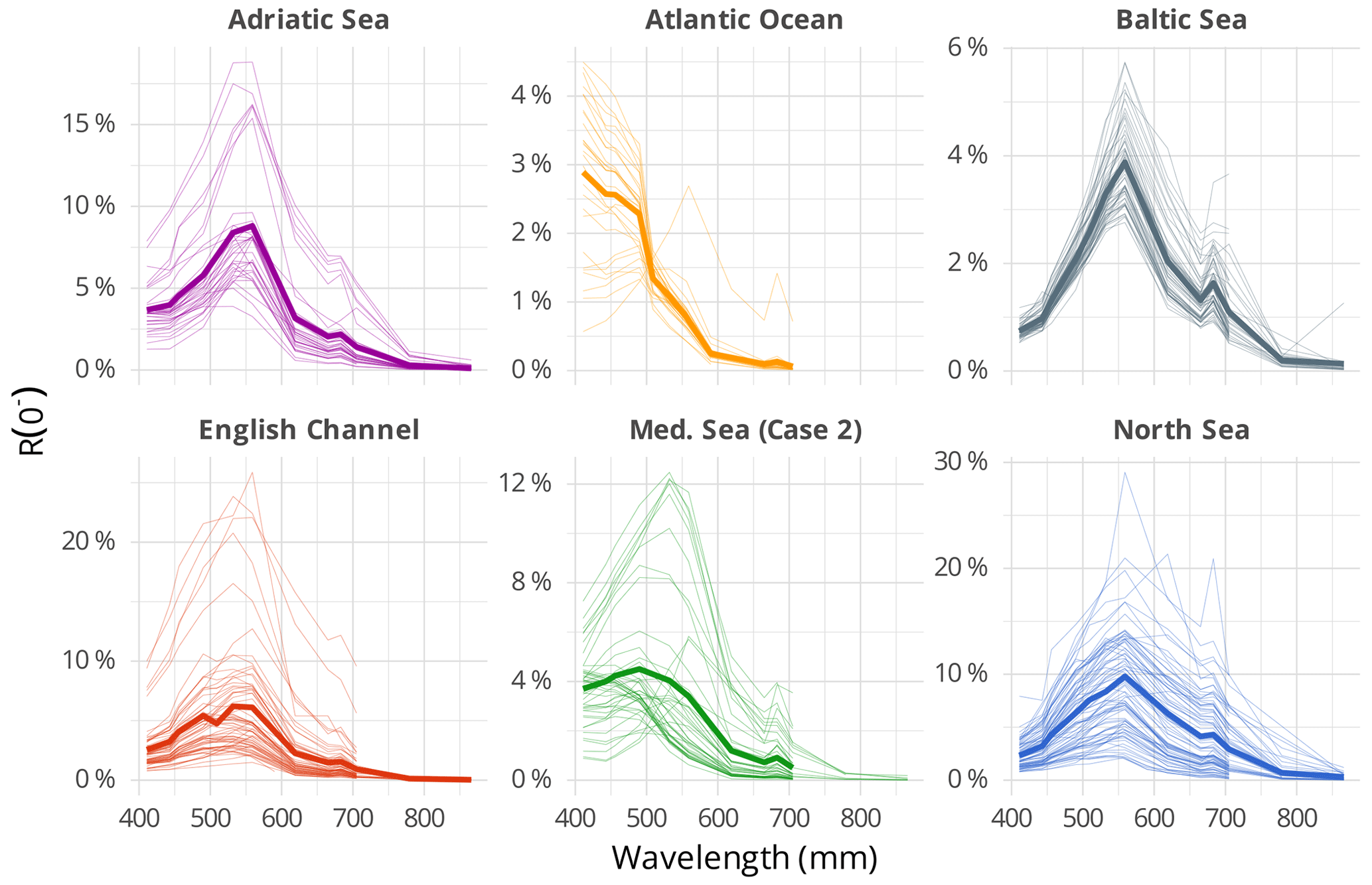
Figure 7Subsurface reflectance R (0−) across the sampled areas. The thick lines represent the regional averages. Note that R (0−) at wavelengths above 705 nm could only be derived from helicopter-based measurements. Please also note that the y axes are adjusted to the data presented within each subplot.
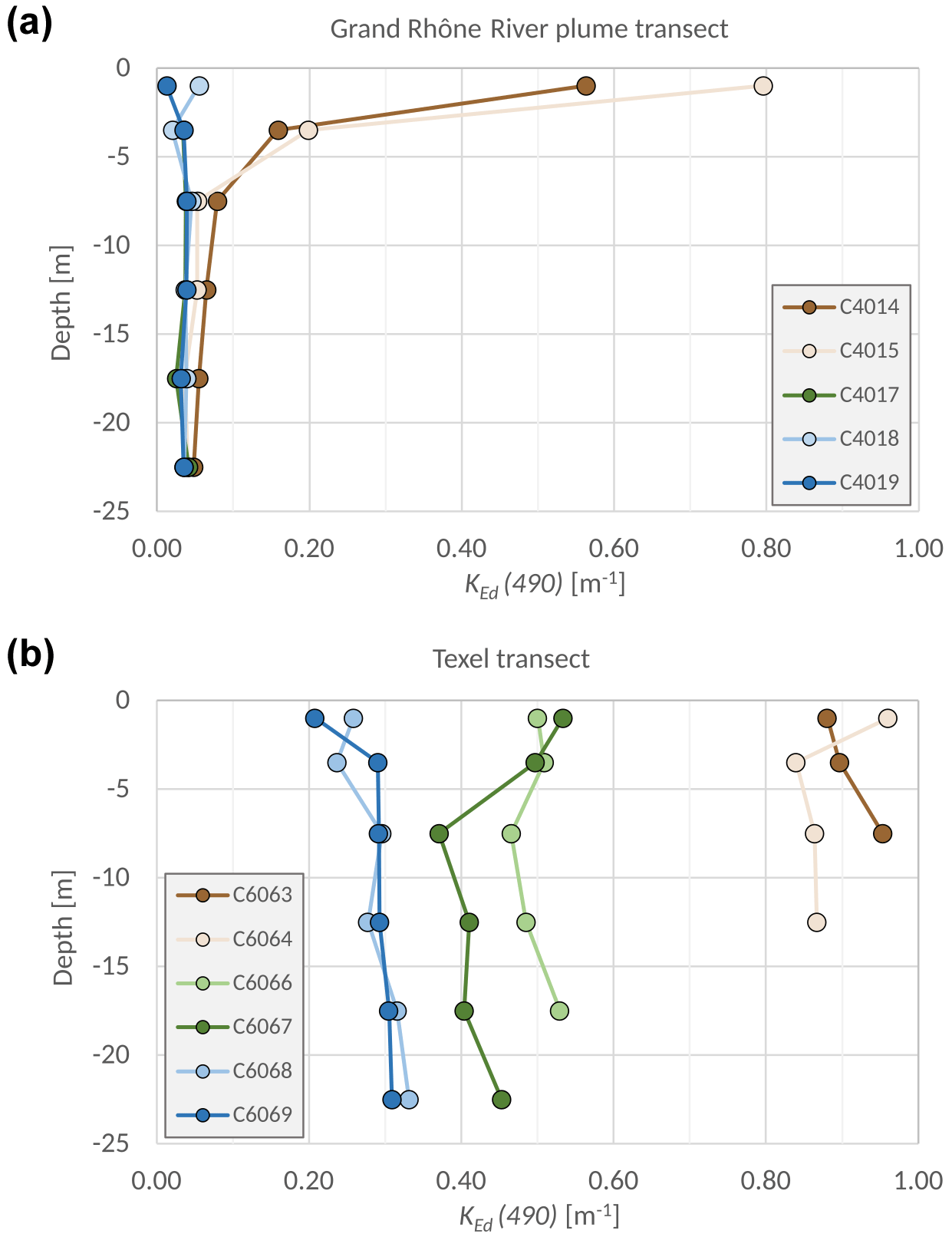
Figure 8(a) KEd(490) profiles taken in the Gulf of Lion on 30 September 1997 along a transect extending from site C4014 located ca. 5 km to the west of the mouth of the main Rhône branch (Grand Rhône) to site C4019 located some 20 km further south in clear Mediterranean waters. (b) KEd(490) profiles taken in the North Sea on 12 September 1998 along a transect extending from site C6063 close to the western shore of the island of Texel to site C6069 located ca. 22 km further west in the open North Sea.
4.1.3 AOPs
Subsurface reflectance R (0−) for all COASTℓOOC sites is shown in Fig. 7, reflecting the fundamental differences in the bio-optical properties of the different areas visited. For example, due to enhanced CDOM absorption, reflectance in the blue part of the spectrum is generally low at the Baltic Sea sites, while it is higher in the Case-1 waters encountered in the Atlantic Ocean or the Mediterranean Sea. In the red and NIR, very high reflectance values are observed in the sediment-rich Case-2 waters of the North Sea and the English Channel.
Sample profiles of the diffuse attenuation coefficient at a vertical resolution between 2.0 m close to the surface and 5.0 m underneath are shown in Fig. 8 for two transition zones ranging from turbid waters close to the coast to clearer waters offshore. Figure 8a shows values along a transect taken in the Gulf of Lion on 30 September 1997 from site C4014 located ca. 5 km to the west of the mouth of the main Rhône branch (Grand Rhône) to site C4019 some 20 km further south in clear Mediterranean waters. While at the offshore sites C4017 to C4019 adopts low values between ca. 0.02 and 0.05 m−1 reflecting clear-water conditions, sites C4014 and C4015 are strongly influenced by the Rhône River plume, resulting in reaching values of up to 0.8 m−1 in the surface layer. The turbid Rhône freshwater floats on top of denser and clearer Mediterranean seawater, resulting in a strong stratification. Figure 8b shows a similar transect taken in the North Sea on 12 September 1998 extending from site C6063 close to the western shore of Texel to site C6069 located ca. 22 km further west in the open North Sea. Again, there is a distance-to-coast-dependent decrease in values likely related to reduced turbidity, from ca. 0.8 to 1.0 m−1 close to the coast down to values of ca. 0.2 to 0.3 m−1 offshore. In contrast to the transect in the Gulf of Lion, no obvious stratification is observed: values are rather homogeneously distributed over the entire water column, pointing to effective mixing.
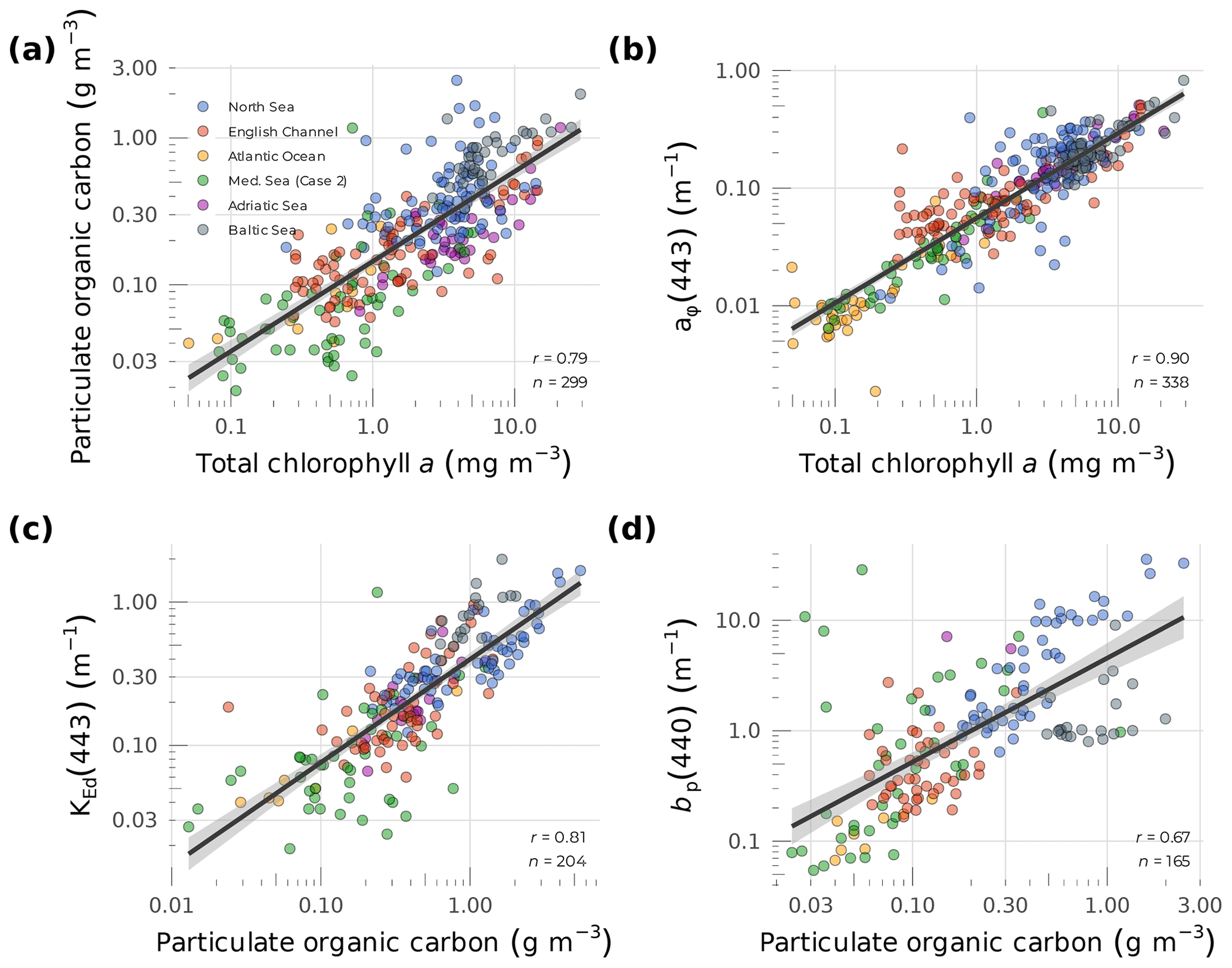
Figure 9Scatterplots showing relationships among different selected variables. (a) Particulate organic carbon (POC) and (b) phytoplankton absorption at 443 nm (aϕ(443)) against total chlorophyll a. (c) Downward irradiance at 443 nm and (d) particulate scattering at 440 nm against particulate organic carbon. The red lines show the linear relationships between the variables. The shaded gray areas represent the 95 % confidence intervals around the fitted models.
4.2 Co-variability across bio-optical measurements
Few research papers have previously shown how optically significant components and AOPs and IOPs measured during the COASTℓOOC missions co-varied (Ferrari, 2000; Ferrari et al., 2003; Babin, 2003; Babin et al., 2003a). In this section, a brief overview of selected pairwise relationships is presented. Total chlorophyll a co-varies with POC (Fig. 4), and the relationship was highly variable (Fig. 9a). While the global Pearson correlation is 0.79 (n=299), it ranged between 0.36 in the North Sea (n=88) and 0.78 in the Adriatic Sea (n=37), showing that optically significant components do not necessarily co-vary altogether. Likewise, the global Pearson correlation between aϕ and total chlorophyll a (Fig. 9b) was relatively high (r=0.90, n=338). The lowest and highest correlations were observed in the North Sea (r=0.69, n=88) and the Adriatic Sea (r=0.91, n=38), respectively. POC concentration is well known to be an important driver of both IOPs and AOPs in aquatic ecosystems (Stramski et al., 2008; Cetinić et al., 2012). Unsurprisingly, positive correlations were observed between POC and (Fig. 9c, r=0.81, n=204) and bp(440) (Fig. 9d, r=0.67, n=165).
Based on the size–reactivity continuum model proposed by Benner and Amon (2015), physicochemical and photochemical processes shape the size distribution of organic matter along the aquatic continuum and determine the contrasted intrinsic nature of the particles for each type of ecosystem. This is likely one key reason explaining why the observed relationships are quite variable across the different sampled ecosystems (Fig. 9). For example, in coastal areas (e.g., the Baltic Sea, Fig. 1), the POC content is generally influenced by large humic organic particles drained by rivers from the surrounding watershed (Babin et al., 2003a). Consequently, in these areas, POC concentration (Fig. 4b), absorption (Fig. 5), and downward attenuation coefficients (Fig. 9c) were higher than in other sampled areas. In contrast, the stations that were farther away from the coast (such as the Atlantic Sea, Fig. 1) had lower POC concentrations (Fig. 4b) and absorption (Fig. 5).
The COASTℓOOC data are provided as a collection of comma-separated value (.csv) files that regroup measurements associated with each measurement. The processed and tidied version of the data is hosted at SEANOE (SEA scieNtific Open data Edition) under the CC-BY license (https://doi.org/10.17882/93570, Massicotte et al., 2023). To aid the user in merging these files, there is a lookup table file designated station list (https://www.seanoe.org/data/00824/93570/data/100311.csv, Massicotte, 2023c) that can serve as a table to join the data together based on the station's unique identifier. Table 1 shows the complete list of available measurements. Please note that the actual filenames (e.g., /100311.csv) are assigned by SEANOE during the upload process and cannot be altered. All statistical analyses were performed in R version 4.3.0 (R Core Team, 2023). The code used to produce the figures and the analysis presented in this paper is available under the GNU GPLv3 license (https://doi.org/10.5281/zenodo.8091717, Massicotte, 2023b). Irradiance depth merging was done with an Interactive Data Language (IDL) code available under the Creative Commons Attribution 3.0 Germany license (https://doi.org/10.5281/zenodo.8096682, Fell, 2023). Note that there are plans to update and further improve the current dataset. More data will likely be recovered from the backup archives, most prominently AC9 measurements to derive in situ vertical profiles of a, bp, and c. Intended improvements to radiometer processing comprise (not exhaustively) a better dark-current correction, the application of a self-shading correction, a more accurate treatment of the air–sea transmission of downward irradiance (Ed), and a closer look at uncertainties. Any update of the COASTℓOOC dataset will be made publicly available through SEANOE.
The consolidated and quality-controlled data collected during the COASTℓOOC oceanographic expeditions offer, even if collected more than 20 years ago, many possibilities for better understanding the bio-optical dynamics along the land-to-sea gradient where optically complex water drained from watersheds mixes with seawater. To date, nearly 40 peer-reviewed studies have made use of the COASTℓOOC dataset to develop remote-sensing algorithms and to study the optical properties of seawater across the coastal to open-ocean gradient (see Table A1). This now consolidated and easily accessible dataset will facilitate future development and evaluation of new bio-optical models adapted for optically complex waters. In this paper, only a subset of variables has been presented. The reader is referred to Table 1 for a complete list and description of variables collected during the COASTℓOOC expeditions.
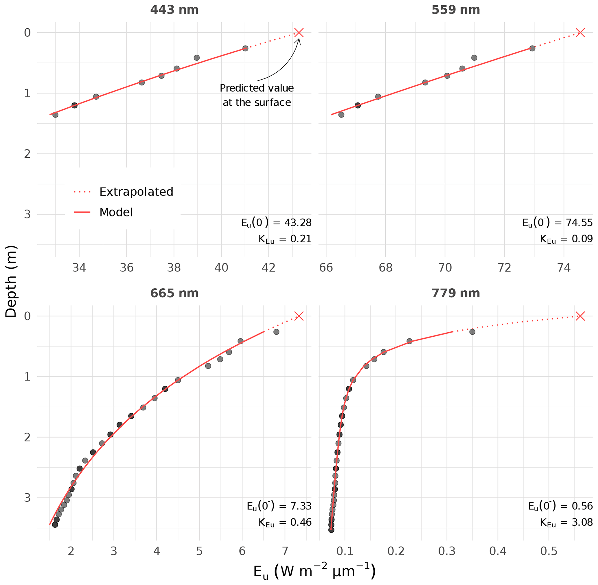
Figure A1Example of extrapolation of the upward irradiance toward the sea surface (station C3004000). The irradiance values just below the sea surface (red crosses, Eu (0−)) and the corresponding diffuse attenuation coefficient for the topmost water layer are specified in the figures. The full lines represent the interpolated values, whereas the dashed lines show extrapolation values up to the sea surface.
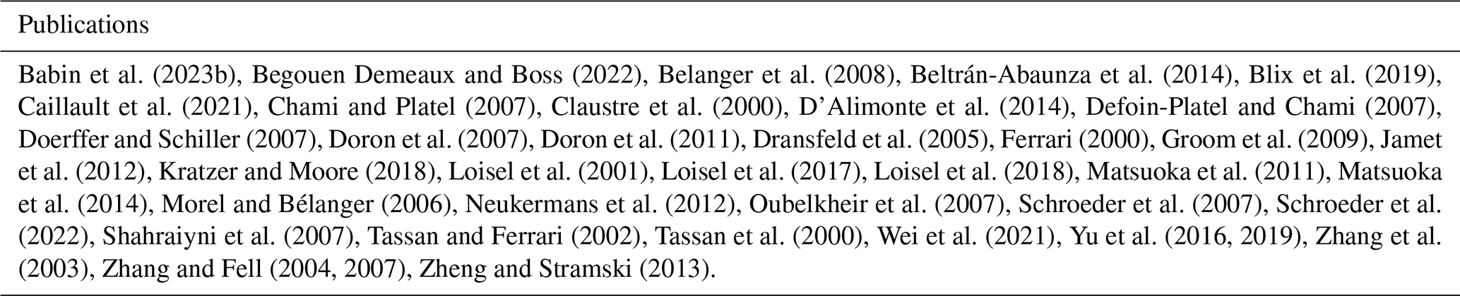
Table A1Scientific articles in peer-reviewed journals using or referencing COASTℓOOC.
Conceptualization: MB. Formal analysis: FF, DD, VFS, MB. Investigation: MB, FF, VFS. Software: DD (AC9), FF (radiometry), VFS (data acquisition and preprocessing). Writing: PM with support from all the co-authors.
The contact author has declared that none of the authors has any competing interests.
Publisher's note: Copernicus Publications remains neutral with regard to jurisdictional claims in published maps and institutional affiliations.
Many people contributed to the generation of the COASTℓOOC database as described herein, be it by contributing to project implementation, supporting field campaigns, performing laboratory work, or providing scientific guidance. In this respect, we would like especially to thank James Aiken, Jean-François Berthon, Annick Bricaud, Hervé Claustre, Roland Doerffer, Giovanni Massimo Ferrari, Hans Hakvoort, Geir Johnsen, Khadija Oubelkheir, Matt Pinkerton, Rainer Reuter, Marcel Wernand, and Grigor Obolensky. We are also grateful to the crews of the ships (NO Thetis-2, RV Poseidon, and RV Victor Hensen) and the helicopter (Commerc'Air SA) we used for collecting the field data.
This paper was edited by Giuseppe M. R. Manzella and reviewed by Emmanuel Boss, Jenny Lovell, and David McKee.
Aiken, J., Antoine, D., Babin, M., Barth, H., Bricaud, A., Chauton, M., Claustre, H., Doerffer, R., Dowell, M., Fell, F., Ferrari, M., Fischer, J., Fournier-Sicre, Vincent, Hakvoort, H., Hoepffner, N., Johnsen, G., Montagner, F., Moore, G., Morel, A., Obolensky, G., Olbert, C., Pinkerton, M., Reuter, R., Sakshaug, E., and Wernand, M.: COASTLOOC (COAstal Surveillance Through Observation of Ocean Colour) Final Report, Tech. rep., Zenodo, https://doi.org/10.5281/ZENODO.7428384, 2000. a, b
Antoine, D., André, J.-M., and Morel, A.: Oceanic Primary Production: 2. Estimation at Global Scale from Satellite (Coastal Zone Color Scanner) Chlorophyll, Global Biogeochem. Cy., 10, 57–69, https://doi.org/10.1029/95GB02832, 1996. a
Babin, M.: Variations in the Light Absorption Coefficients of Phytoplankton, Nonalgal Particles, and Dissolved Organic Matter in Coastal Waters around Europe, J. Geophys. Res., 108, 3211, https://doi.org/10.1029/2001JC000882, 2003. a, b, c, d, e, f, g
Babin, M., Morel, A., Fournier-Sicre, V., Fell, F., and Stramski, D.: Light Scattering Properties of Marine Particles in Coastal and Open Ocean Waters Asrelated to the Particle Mass Concentration, Limnol. Oceanogr., 48, 843–859, https://doi.org/10.4319/lo.2003.48.2.0843, 2003a. a, b
Babin, M., Stramski, D., Ferrari, G. M., Claustre, H., Bricaud, A., Obolensky, G., and Hoepffner, N.: Variations in the light absorption coefficients of phytoplankton, nonalgal particles, and dissolved organic matter in coastal waters around Europe, J. Geophys. Res.-Oceans, 108, 3211, https://doi.org/10.1029/2001JC000882, 2003b. a
Begouen Demeaux, C. and Boss, E.: Validation of Remote-Sensing Algorithms for Diffuse Attenuation of Downward Irradiance Using BGC-Argo Floats, Remote Sens., 14, 4500, https://doi.org/10.3390/rs14184500, 2022. a
Belanger, S., Babin, M., and Larouche, P.: An empirical ocean color algorithm for estimating the contribution of chromophoric dissolved organic matter to total light absorption in optically complex waters, J. Geophys. Res.-Oceans, 113, C04027, https://doi.org/10.1029/2007JC004436, 2008. a
Beltrán-Abaunza, J. M., Kratzer, S., and Brockmann, C.: Evaluation of MERIS products from Baltic Sea coastal waters rich in CDOM, Ocean Sci., 10, 377–396, https://doi.org/10.5194/os-10-377-2014, 2014. a
Benner, R. and Amon, R. M.: The Size-Reactivity Continuum of Major Bioelements in the Ocean, Annu. Rev. Mar. Sci., 7, 185–205, https://doi.org/10.1146/annurev-marine-010213-135126, 2015. a
Blix, K., Li, J., Massicotte, P., and Matsuoka, A.: Developing a new machine-learning algorithm for estimating chlorophyll-a concentration in optically complex waters: A case study for high northern latitude waters by using Sentinel 3 OLCI, Remote Sens., 11, 2076, https://doi.org/10.3390/rs11182076, 2019. a
Bricaud, A., Morel, A., and Prieur, L.: Absorption by Dissolved Organic Matter of the Sea (Yellow Substance) in the UV and Visible Domains, Limnol. Oceanogr., 26, 43–53, https://doi.org/10.4319/lo.1981.26.1.0043, 1981. a
Caillault, K., Roupioz, L., and Viallefont-Robinet, F.: Modelling of the optical signature of oil slicks at sea for the analysis of multi-and hyperspectral VNIR-SWIR images, Optics Express, 29, 18224–18242, 2021. a
Carr, M.-E., Friedrichs, M. A., Schmeltz, M., Noguchi Aita, M., Antoine, D., Arrigo, K. R., Asanuma, I., Aumont, O., Barber, R., Behrenfeld, M., Bidigare, R., Buitenhuis, E. T., Campbell, J., Ciotti, A., Dierssen, H., Dowell, M., Dunne, J., Esaias, W., Gentili, B., Gregg, W., Groom, S., Hoepffner, N., Ishizaka, J., Kameda, T., Le Quéré, C., Lohrenz, S., Marra, J., Mélin, F., Moore, K., Morel, A., Reddy, T. E., Ryan, J., Scardi, M., Smyth, T., Turpie, K., Tilstone, G., Waters, K., and Yamanaka, Y.: A Comparison of Global Estimates of Marine Primary Production from Ocean Color, Deep-Sea Res. Pt. II, 53, 741–770, https://doi.org/10.1016/j.dsr2.2006.01.028, 2006. a
Cetinić, I., Perry, M. J., Briggs, N. T., Kallin, E., D'Asaro, E. A., and Lee, C. M.: Particulate Organic Carbon and Inherent Optical Properties during 2008 North Atlantic Bloom Experiment: POC AND OPTICS-NAB08, J. Geophys. Res.-Oceans, 117, C06028, https://doi.org/10.1029/2011JC007771, 2012. a
Chami, M. and Platel, M. D.: Sensitivity of the retrieval of the inherent optical properties of marine particles in coastal waters to the directional variations and the polarization of the reflectance, J. Geophys. Res.-Oceans, 112, C05037, https://doi.org/10.1029/2006JC003758, 2007. a
Claustre, H., Fell, F., Oubelkheir, K., Prieur, L., Sciandra, A., Gentili, B., and Babin, M.: Continuous monitoring of surface optical properties across a geostrophic front: Biogeochemical inferences. Limnol. Oceanogr., 45(2), 309–321, 2000. a
Cole, J. J., Prairie, Y. T., Caraco, N. F., McDowell, W. H., Tranvik, L. J., Striegl, R. G., Duarte, C. M., Kortelainen, P., Downing, J. A., Middelburg, J. J., and Melack, J.: Plumbing the Global Carbon Cycle: Integrating Inland Waters into the Terrestrial Carbon Budget, Ecosystems, 10, 172–185, https://doi.org/10.1007/s10021-006-9013-8, 2007. a
D'Alimonte, D., Zibordi, G., Kajiyama, T., and Berthon, J. F.: Comparison between MERIS and regional high-level products in European seas, Remote Sens. Environ., 140, 378–395, 2014. a
Defoin-Platel, M. and Chami, M.: How ambiguous is the inverse problem of ocean color in coastal waters?, J. Geophys. Res.-Oceans, 112, C03004, https://doi.org/10.1029/2006JC003847, 2007. a
Doerffer, R. and Schiller, H.: The MERIS Case 2 water algorithm, Int. J. Remote Sens., 28, 517–535, 2007. a
Doron, M., Babin, M., Mangin, A., and Hembise, O.: Estimation of light penetration, and horizontal and vertical visibility in oceanic and coastal waters from surface reflectance, J. Geophys. Res.-Oceans, 112, C06003, https://doi.org/10.1029/2006JC004007, 2007. a
Doron, M., Babin, M., Hembise, O., Mangin, A., and Garnesson, P.: Ocean transparency from space: Validation of algorithms estimating Secchi depth using MERIS, MODIS and SeaWiFS data, Remote Sens. Environ., 115, 2986–3001, 2011. a
Dransfeld, S., Tatnall, A. R., Robinson, I. S., and Mobley, C. D.: Prioritizing ocean colour channels by neural network input reflectance perturbation, Int. J. Remote Sens., 26, 1043–1048, 2005. a
Fell, F.: Oceanic Irradiance Profile Processing, Zenodo [code], https://doi.org/10.5281/zenodo.8096682, 2023. a
Ferrari, G. M.: The Relationship between Chromophoric Dissolved Organic Matter and Dissolved Organic Carbon in the European Atlantic Coastal Area and in the West Mediterranean Sea (Gulf of Lions), Mar. Chem., 70, 339–357, https://doi.org/10.1016/S0304-4203(00)00036-0, 2000. a, b, c, d
Ferrari, G. M., Bo, F. G., and Babin, M.: Geo-Chemical and Optical Characterizations of Suspended Matter in European Coastal Waters, Estuar. Coast. Shelf S., 57, 17–24, https://doi.org/10.1016/S0272-7714(02)00314-1, 2003. a, b, c
GEBCO Bathymetric Compilation Group 2021: The GEBCO_2021 Grid – a Continuous Terrain Model of the Global Oceans and Land, National Oceanography Centre [data set], https://doi.org/10.5285/C6612CBE-50B3-0CFF-E053-6C86ABC09F8F, 2021. a
Gordon, H. R. and Morel, A. Y.: Remote Assessment of Ocean Color for Interpretation of Satellite Visible Imagery: A Review, Springer US, New York, NY, ISBN 978-1-4684-6280-7, 1983. a
Groom, S., Martinez-Vicente, V., Fishwick, J., Tilstone, G., Moore, G., Smyth, T., and Harbour, D.: The western English Channel observatory: Optical characteristics of station L4, J. Marine Syst., 77, 278–295, 2009. a
Guthrie, W. F.: NIST/SEMATECH e-Handbook of Statistical Methods (NIST Handbook 151), National Institute of Standards and Technology (NIST), Gaithersburg, MD USA, https://doi.org/10.18434/M32189, 2012. a
Hedges, J., Keil, R., and Benner, R.: What Happens to Terrestrial Organic Matter in the Ocean?, Org. Geochem., 27, 195–212, https://doi.org/10.1016/S0146-6380(97)00066-1, 1997. a
Jamet, C., Loisel, H., and Dessailly, D.: Retrieval of the spectral diffuse attenuation coefficient Kd(λ) in open and coastal ocean waters using a neural network inversion, J. Geophys. Res.-Oceans, 117, C10023, https://doi.org/10.1029/2012JC008076, 2012. a
Jerlov, N. G.: Optical Oceanography, Limnol. Oceanogr., 13, 731–732, https://doi.org/10.4319/lo.1968.13.4.0731, 1968. a
Kratzer, S. and Moore, G.: Inherent optical properties of the baltic sea in comparison to other seas and oceans, Remote Sens., 10, 418, https://doi.org/10.3390/rs10030418, 2018. a
Lee, Z., Carder, K. L., Mobley, C. D., Steward, R. G., and Patch, J. S.: Hyperspectral Remote Sensing for Shallow Waters. I. A Semianalytical Model, Appl. Optics, 37, 6329, https://doi.org/10.1364/AO.37.006329, 1998. a
Loisel, H., Stramski, D., Mitchell, B. G., Fell, F., Fournier-Sicre, V., Lemasle, B., and Babin, M.: Comparison of the ocean inherent optical properties obtained from measurements and inverse modeling, Appl. Optics, 40, 2384–2397, 2001. a
Loisel, H., Vantrepotte, V., Ouillon, S., Ngoc, D. D., Herrmann, M., Tran, V., Mériaux, X., Dessailly, D., Jamet, C., Duhaut, T., Nguyen, H. H., and Van Nguyen, T.: Assessment and analysis of the chlorophyll-a concentration variability over the Vietnamese coastal waters from the MERIS ocean color sensor (2002–2012), Remote Sens. Environ., 190, 217–232, 2017. a
Loisel, H., Stramski, D., Dessailly, D., Jamet, C., Li, L., and Reynolds, R. A.: An inverse model for estimating the optical absorption and backscattering coefficients of seawater from remote-sensing reflectance over a broad range of oceanic and coastal marine environments, J. Geophys. Res.-Oceans, 123, 2141–2171, 2018. a
Massicotte, P.: PMassicotte/Coastlooc_data_paper: V1.0.0, Zenodo [code], https://doi.org/10.5281/ZENODO.7708653, 2023a.
Massicotte, P.: PMassicotte/coastlooc_data_paper: ESSD revision round 1 (v1.1.0), Zenodo [code], https://doi.org/10.5281/zenodo.8091717, 2023b. a
Massicotte, P.: The COASTLOOC dataset [data set], https://www.seanoe.org/data/00824/93570/data/100311.csv, last access: 3 March 2023c. a
Massicotte, P., Stedmon, C., and Markager, S.: Spectral Signature of Suspended Fine Particulate Material on Light Absorption Properties of CDOM, Mar. Chem., 196, 98–106, https://doi.org/10.1016/j.marchem.2017.07.005, 2017. a, b
Massicotte, P., Babin, M., Fell, F., Fournier-Sicre, V., and Doxaran, D.: The COASTLOOC Project Dataset, SEANOE [data set], https://doi.org/10.17882/93570, 2023. a, b
Matsuoka, A., Hill, V., Huot, Y., Babin, M., and Bricaud, A.: Seasonal variability in the light absorption properties of western Arctic waters: Parameterization of the individual components of absorption for ocean color applications, J. Geophys. Res.-Oceans, 116, 3131–3147, https://doi.org/10.1029/2009JC005594, 2011. a
Matsuoka, A., Babin, M., Doxaran, D., Hooker, S. B., Mitchell, B. G., Bélanger, S., and Bricaud, A.: A synthesis of light absorption properties of the Arctic Ocean: application to semianalytical estimates of dissolved organic carbon concentrations from space, Biogeosciences, 11, 3131–3147, https://doi.org/10.5194/bg-11-3131-2014, 2014. a
Morel, A. and Bélanger, S.: Improved Detection of Turbid Waters from Ocean Color Sensors Information, Remote Sens. Environ., 102, 237–249, https://doi.org/10.1016/j.rse.2006.01.022, 2006. a, b
Morel, A. and Prieur, L.: Analysis of Variations in Ocean Color: Ocean Color Analysis, Limnol. Oceanogr., 22, 709–722, https://doi.org/10.4319/lo.1977.22.4.0709, 1977. a, b
Neukermans, G., Loisel, H., Mériaux, X., Astoreca, R., and McKee, D.: In situ variability of mass-specific beam attenuation and backscattering of marine particles with respect to particle size, density, and composition, Limnol. Oceanogr., 57, 124–144, 2012. a
O'Reilly, J. E. and Werdell, P. J.: Chlorophyll Algorithms for Ocean Color Sensors - OC4, OC5 & OC6, Remote Sens. Environ., 229, 32–47, https://doi.org/10.1016/j.rse.2019.04.021, 2019. a
Oubelkheir, K., Claustre, H., Bricaud, A., and Babin, M.: Partitioning total spectral absorption in phytoplankton and colored detrital material contributions, Limnol. Oceanogr.-Methods, 5, 384–395, 2007. a
R Core Team: R: A Language and Environment for Statistical Computing, R Foundation for Statistical Computing, Vienna, Austria, 2023. a
Sathyendranath, S.: Remote Sensing of Ocean Colour in Coastal, and Other Optically-Complex, Waters, Reports of the International Ocean-Colour Coordinating Group, No. 3, IOCCG, Dartmouth, Canada, 2000. a, b
Schroeder, T., Behnert, I., Schaale, M., Fischer, J., and Doerffer, R.: Atmospheric correction algorithm for MERIS above case-2 waters, Int. J. Remote Sens., 28, 1469–1486, 2007. a
Schroeder, T., Schaale, M., Lovell, J., and Blondeau-Patissier, D.: An ensemble neural network atmospheric correction for Sentinel-3 OLCI over coastal waters providing inherent model uncertainty estimation and sensor noise propagation, Remote Sens. Environ., 270, 112848, https://doi.org/10.1016/j.rse.2021.112848, 2022. a
Shahraiyni, T. H., Schaale, M., Fell, F., Fischer, J., Preusker, R., Vatandoust, M., Shouraki, B. S., Tajrishy, M., Khodaparast, H., and Tavakoli, A.: Application of the Active Learning Method for the estimation of geophysical variables in the Caspian Sea from satellite ocean colour observations, Int. J. Remote Sens., 28, 4677–4683, 2007. a
Stramski, D., Reynolds, R. A., Babin, M., Kaczmarek, S., Lewis, M. R., Röttgers, R., Sciandra, A., Stramska, M., Twardowski, M. S., Franz, B. A., and Claustre, H.: Relationships between the surface concentration of particulate organic carbon and optical properties in the eastern South Pacific and eastern Atlantic Oceans, Biogeosciences, 5, 171–201, https://doi.org/10.5194/bg-5-171-2008, 2008. a
Sugihara, S., Kishino, M., and Okami, N.: Contribution of Raman Scattering to Upward Irradiance in the Sea, Journal of the Oceanographical Society of Japan, 40, 397–404, https://doi.org/10.1007/BF02303065, 1984. a
Tassan, S. and Ferrari, G. M.: An Alternative Approach to Absorption Measurements of Aquatic Particles Retained on Filters, Limnol. Oceanogr., 40, 1358–1368, https://doi.org/10.4319/lo.1995.40.8.1358, 1995. a
Tassan, S. and Ferrari, G. M.: Measurement of Light Absorption by Aquatic Particles Retained on Filters: Determination of the Optical Pathlength Amplification by the `Transmittance-Reflectance' Method, J. Plankton Res., 20, 1699–1709, https://doi.org/10.1093/plankt/20.9.1699, 1998. a
Tassan, S. and Ferrari, G. M.: A sensitivity analysis of the “Transmittance–Reflectance” method for measuring light absorption by aquatic particles, J. Plankton Res., 24, 757–774, 2002. a
Tassan, S. and Ferrari, G. M.: Variability of Light Absorption by Aquatic Particles in the Near-Infrared Spectral Region, Appl. Optics, 42, 4802, https://doi.org/10.1364/AO.42.004802, 2003. a
Tassan, S., Ferrari, G. M., Bricaud, A., and Babin, M.: Variability of the amplification factor of light absorption by filter-retained aquatic particles in the coastal environment, J. Plankton Res., 22, 659–668, 2000. a
Van Der Linde, D.: Protocol for Determination of Total Suspended Matter in Oceans and Coastal Zones, Technical Note No. 1.98.182, CEC-JRC, Ispra, Italy, 8 pp., 1998. a
Vargas, M., Brown, C. W., and Sapiano, M. R. P.: Phenology of Marine Phytoplankton from Satellite Ocean Color Measurements, Geophys. Res. Lett., 36, L01608, https://doi.org/10.1029/2008GL036006, 2009. a
Vidussi, F., Claustre, H., Bustillos-Guzmàn, J., Cailliau, C., and Marty, J.-C.: Determination of Chlorophylls and Carotenoids of Marine Phytoplankton: Separation of Chlorophyll a from Divinylchlorophyll a and Zeaxanthin from Lutein, J. Plankton Res., 18, 2377–2382, https://doi.org/10.1093/plankt/18.12.2377, 1996. a
Wei, J., Wang, M., Jiang, L., Yu, X., Mikelsons, K., and Shen, F.: Global estimation of suspended particulate matter from satellite ocean color imagery, J. Geophys. Res.-Oceans, 126, e2021JC017303, https://doi.org/10.1029/2021JC017303, 2021. a
Yu, X., Salama, M. S., Shen, F., and Verhoef, W.: Retrieval of the diffuse attenuation coefficient from GOCI images using the 2SeaColor model: A case study in the Yangtze Estuary, Remote Sens. Environ., 175, 109–119, 2016. a
Yu, X., Lee, Z., Shen, F., Wang, M., Wei, J., Jiang, L., and Shang, Z.: An empirical algorithm to seamlessly retrieve the concentration of suspended particulate matter from water color across ocean to turbid river mouths, Remote Sens. Environ., 235, 111491, https://doi.org/10.1016/j.rse.2019.111491, 2019. a
Zhang, T. and Fell, F.: An approach to improving the retrieval accuracy of oceanic constituents in Case II waters, J. Ocean U. China, 3, 220–224, 2004. a
Zhang, T. and Fell, F.: An empirical algorithm for determining the diffuse attenuation coefficient Kd in clear and turbid waters from spectral remote sensing reflectance, Limnol. Oceanogr.-Methods, 5, 457–462, 2007. a
Zhang, T., Fell, F., Liu, Z. S., Preusker, R., Fischer, J., and He, M. X.: Evaluating the performance of artificial neural network techniques for pigment retrieval from ocean color in Case I waters, J. Geophys. Res.-Oceans, 108, 3286, https://doi.org/10.1029/2002JC001638, 2003. a
Zheng, G. and Stramski, D.: A model based on stacked-constraints approach for partitioning the light absorption coefficient of seawater into phytoplankton and non-phytoplankton components, J. Geophys. Res.-Oceans, 118, 2155–2174, 2013. a