A long-term monthly surface water storage dataset for the Congo basin from 1992 to 2015

The spatio-temporal variation of surface water storage (SWS) in the Congo River basin (CRB), the second-largest watershed in the world, remains widely unknown. In this study, satellite-derived observations are combined to estimate SWS dynamics at the CRB and sub-basin scales over 1992–2015. Two methods are employed. The first one combines surface water extent (SWE) from the Global Inundation Extent from Multi-Satellite (GIEMS-2) dataset and the long-term satellite-derived surface water height from multi-mission radar altimetry. The second one, based on the hypsometric curve approach, combines SWE from GIEMS-2 with topographic data from four global digital elevation models (DEMs), namely the Terra Advanced Spaceborne Thermal Emission and Reflection Radiometer (ASTER), Advanced Land Observing Satellite (ALOS), Multi-Error-Removed Improved Terrain (MERIT), and Forest And Buildings removed Copernicus DEM (FABDEM). The results provide SWS variations at monthly time steps from 1992 to 2015 characterized by a strong seasonal and interannual variability with an annual mean amplitude of $\sim \mathrm{101}\pm \mathrm{23}$ km³. The Middle Congo sub-basin shows a higher mean annual amplitude ($\sim \mathrm{71}\pm \mathrm{15}$ km³). The comparison of SWS derived from the two methods and four DEMs shows an overall fair agreement. The SWS estimates are assessed against satellite precipitation data and in situ river discharge and, in general, a relatively fair agreement is found between the three hydrological variables at the basin and sub-basin scales (linear correlation coefficient >0.5). We further characterize the spatial distribution of the major drought that occurred across the basin at the end of 2005 and in early 2006. The SWS estimates clearly reveal the widespread spatial distribution of this severe event (∼40 % deficit as compared to their long-term average), in accordance with the large negative anomaly observed in precipitation over that period. This new SWS long-term dataset over the Congo River basin is an unprecedented new source of information for improving our comprehension of hydrological and biogeochemical cycles in the basin. As the datasets used in our study are available globally, our study opens opportunities to further develop satellite-derived SWS estimates at the global scale. The dataset of the CRB's SWS and the related Python code to run the reproducibility of the hypsometric curve approach dataset of SWS are respectively available for download at https://doi.org/10.5281/zenodo.7299823 and https://doi.org/10.5281/zenodo.8011607 (Kitambo et al., 2022b, 2023).

1 Introduction

Freshwater on Earth's ice-free land accounts for only ∼1 % of the total amount of water globally (Vörösmarty et al., 2010; Steffen et al., 2015; Cazenave et al., 2016; Albert et al., 2021). However, terrestrial freshwater is essential to all human needs, ecosystem environments, and biospheric processes. Freshwater on land (excluding ice caps) is stored in various forms, including glaciers, snowpacks, aquifers, the root zone (upper few metres of the soil), and surface waters. The latter include rivers, lakes, artificial reservoirs, wetlands, floodplains, and inundated areas (Boberg, 2005; Zhou et al., 2016). All these continental components are permanently interacting with the atmosphere and oceans, exchanging energy and water fluxes (i.e. precipitation, evaporation, transpiration of the vegetation, heat transfer, and surface and underground runoff) through horizontal and vertical motions characterizing the global water cycle (Trenberth et al., 2007, 2011; Good et al., 2015; Cazenave et al., 2016). These exchanges and the associated storage variations of continental freshwater, specifically surface waters, are key players in the climate system and water resource variability as well as in the global biogeochemical and hydrological cycles (Chahine, 1992; de Marsily, 2005; Oki and Kanae, 2006; Shelton, 2009; Stephens et al., 2020). For instance, despite their small surface coverage (∼6 % of the continents), wetlands and floodplains have a substantial impact on flood flow alteration, sediment stabilization, water quality, groundwater recharge, and discharge (Bullock and Acreman, 2003). The amount of water stored through large floodplains and wetlands is a key component for understanding the exchange between the main river channel and the dissolved and particulate material (sediment and organic matter) (Melack and Forsberg, 2001; Ward et al., 2017). Furthermore, it also acts as a regulator for basin hydrology owning to storage effects along channel reaches (Reis et al., 2017; Wohl, 2021). Additionally, the amount of water stored and flowing through surface water bodies influences the biogeochemical and trace gas exchanges and transport between the atmosphere, land, and the ocean (Richey et al., 2002; Raymond et al., 2013; Hastie et al., 2021).

Surprisingly, in spite of the importance of surface water storage (SWS), our current knowledge about its spatio-temporal variability is still poor, especially at regional and global scales (Mekonnen and Hoekstra, 2016; Cooley et al., 2021). Therefore, there is a fundamental need for the quantification of the storage of surface freshwater on land (Alsdorf et al., 2003, 2007; Rodell et al., 2015; O'Connell, 2017).

Efforts have recently been devoted to measuring SWS for large lakes, reservoirs, rivers, floodplains, and wetlands in large river basins using satellite-derived observations. Papa and Frappart (2021) provide an overview of the recent advances in the quantification of SWS in rivers, floodplains, and wetlands from Earth observations, presenting several studies (e.g. Frappart et al., 2008, 2010, 2012, 2015a, 2018; Papa et al., 2013, 2015; Becker et al., 2018; Tourian et al., 2018; Normandin et al., 2018; Pham-Duc et al., 2020) that characterize the variations in SWS changes in different large river basins. For instance, Frappart et al. (2012) used continuous multi-satellite observations of surface water extent and water level from 2003 to 2007 to monitor monthly variations of SWS in the Amazon River basin and the signature of the exceptional drought of 2005, when the amount of water in rivers and floodplains was found to be ∼70 % below its long-term average. Papa et al. (2013) developed a hypsometric curve approach to derive SWS variations by combining surface extent from the Global Inundation Extent from Multi-Satellite (GIEMS; Prigent et al., 2007) dataset and topographic data from the global digital elevation model from the Advance Spaceborne Thermal Emission and Reflection Radiometer (ASTER). At the basin scale, they showed that the mean annual amplitude of the Amazon SWS is ∼1200 km³ and contributes about half of the annual terrestrial water change as detected by Gravity and Recovery Climate Experiment (GRACE) data (Papa and Frappart, 2021).

Despite being the second-largest river system in the world, in terms of both the drainage area and discharge to the ocean, the Congo River basin (CRB)'s SWS still remains widely unknown. The CRB still hosts extensive floodplains and wetlands such as the well-known Cuvette Centrale region, which stores a large amount of freshwater, playing a crucial role in the sediment dynamics of the river and in the global carbon storage (Datok et al., 2022; Biddulph et al., 2021).

Crowley et al. (2006) estimated terrestrial (surface plus ground) water storage within the Congo basin for the period of April 2002 to May 2006 using GRACE satellite gravity data. The result showed significant seasonal (30±6 mm of equivalent water thickness) and long-term trends, the latter yielding a total loss of ∼280 km³ of water over the 50-month period of analysis. Lee et al. (2011) determined the amount of water annually filling and draining the Congo main wetlands to 111 km³. This was done by using a water balance equation combining several remotely sensed observations (i.e. GRACE, satellite radar altimeter, GPCP, JERS-1, SRTM, and MODIS). Richey et al. (2015) provided a groundwater stress assessment quantifying the relationship between groundwater use and availability in the world's 37 largest aquifer systems using GRACE data. The Congo basin aquifer is characterized as low stress from the renewable groundwater stress ratio. At the basin scale, Becker et al. (2018) further estimated the spatio-temporal variability of SWS by combining surface water extent from GIEMS and radar-altimeter-derived surface water height of rivers at 350 virtual stations (VSs) from the Environmental Satellite (ENVISAT) mission over the period 2003–2007. They reported that the mean annual variations of the CRB's SWS were about 81±24 km³, contributing 19±5 % of the annual variations of GRACE-derived terrestrial water storage. Recently, Frappart et al. (2021) proposed a densification of the network of VSs by including water elevation variations over the floodplains of the Cuvette Centrale and showed that SWS estimates can be much larger than when only VSs over the rivers are used. In parallel, PALSAR observations in InSAR acquisitions were used over the Cuvette Centrale of the Congo in combination with ENVISAT altimetry to establish relationships between water depth and surface water storage and derived absolute surface water storage change over 2002–2011 (Yuan et al., 2017).

Despite these efforts to characterize the CRB's SWS, there is still a lot to unravel about the dynamics of SWS in the basin, leaving major questions open. What are the spatio-temporal dynamics of SWS over long-term periods at CRB basin and sub-basin scales? How are these dynamics modulated by climate variability and what is the SWS behaviour during exceptional drought events?

Earth observation is a unique means to answer these questions and is very useful for monitoring large drainage basin climate and hydrology where in situ information is lacking (Fassoni-Andrade et al., 2021; Kitambo et al., 2022a). Thus, in this study, we use two approaches to estimate, for the first time, the spatio-temporal variations of the CRB's SWS over the period 1992–2015. The first approach (Frappart et al., 2008, 2011, 2012, 2019) is based on the complementarity between the spatio-temporal dynamics of the surface water extent and satellite-derived surface water height. The second approach relies on the methodology developed by Papa et al. (2013) using the relationships between elevation from digital elevation models and surface water extent variations, called the hypsometric curve approach, which enables the estimation of SWS changes.

Section 2 presents the study area. Section 3 describes the datasets and Sect. 4 the methodology used in this study. Section 5 is dedicated to results and validation. An assessment is performed by comparing the developed SWS with other independent datasets such as historic and contemporary river discharge and precipitation data. Section 6 presents an application case of the dataset in which the spatial distribution of the major drought that occurred across the basin at the end of 2005 and in early 2006 is investigated. Section 7 presents the repository from which the SWS dataset can be accessed freely, and finally, Sect. 8 provides the conclusions and future perspectives.

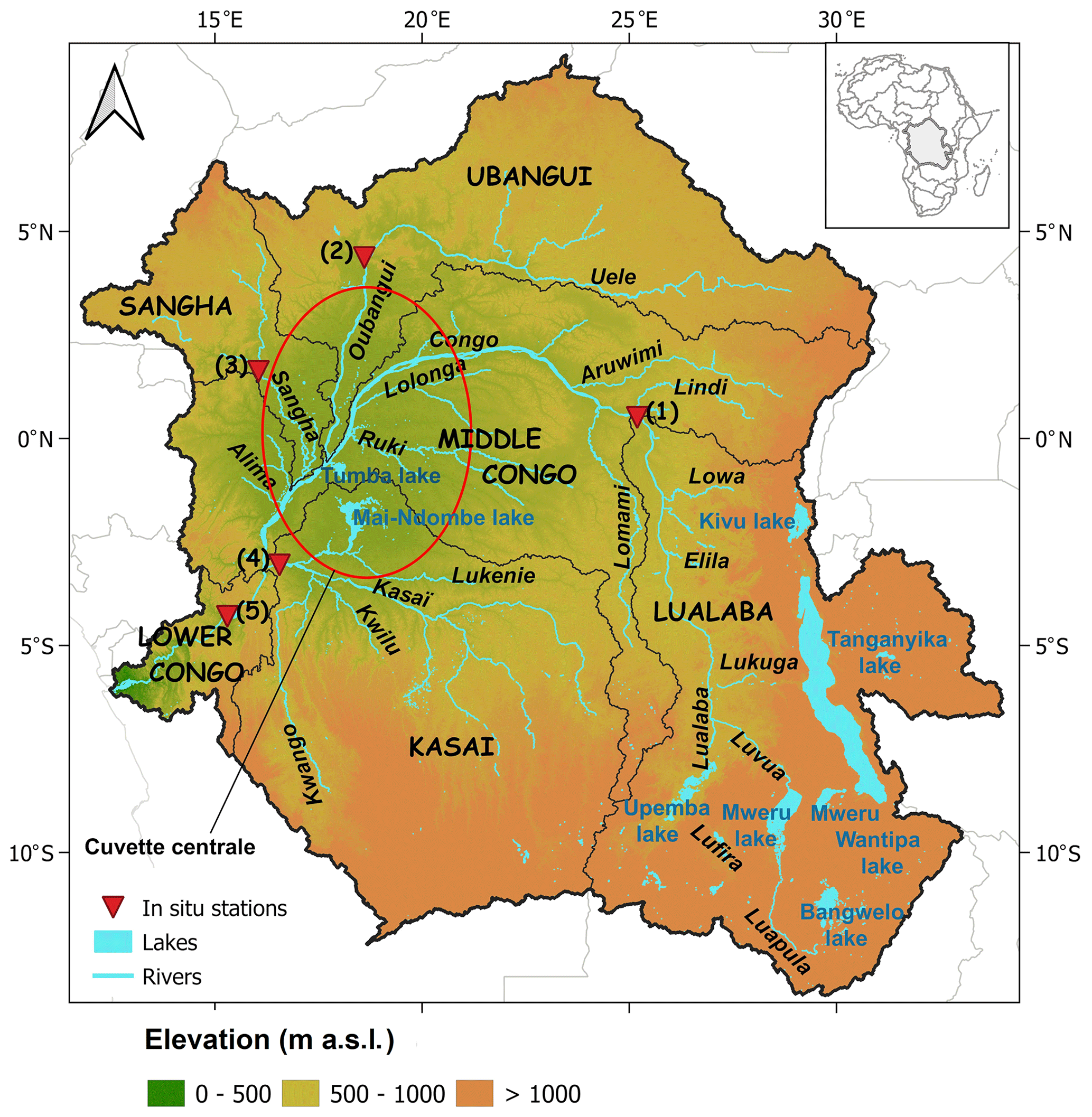
Figure 1 The Congo River basin (CRB) and its main sub-basins (thin dark line) along with the major rivers and lakes (light blue colour). The green portion in the central part circled by red line corresponds to the Cuvette Centrale. The background topography is derived from the Multi-Error-Removed Improved Terrain (MERIT) digital elevation model (DEM). The red triangles display the available in situ gauging stations, with their characteristics reported in Table 2.

2 Study area

The CRB (Fig. 1) represents the second-largest freshwater system in the world, behind the Amazon basin, both in terms of drainage area ($\sim \mathrm{3.7}\times {\mathrm{10}}^{\mathrm{6}}$ km²) and mean annual river discharge (40 500 m³ s⁻¹) (Laraque et al., 2009, 2013). This large basin hosts the Earth's second-largest expanse of tropical forest, covering about 45 % of its area and the world's largest tropical peat carbon storage (∼28 % of the total tropical peat carbon). The vast resources of the basin support the livelihoods of 80 % of the riparian population (Verhegghen et al., 2012; Inogwabini, 2020; White et al., 2021; Crezee et al., 2022). The Congo River flows over 4700 km from its source in the south-eastern part of the Democratic Republic of Congo (DRC) to the Atlantic Ocean, and its drainage area spans over nine countries, the Central African Republic, Cameroon, the Republic of the Congo, Angola, the DRC, Zambia, Tanzania, Rwanda, and Burundi.

The CRB is generally divided into six main sub-basins (Fig. 1) based on the physiography of the basin (Laraque et al., 2020): Lower Congo (south-west), Middle Congo (centre), Sangha (north-west), Ubangui (north-east), Kasaï (southern centre), and Lualaba (south-east). The mean surface air temperature over the basin is estimated to be 25 ^∘C. The average rainfall is 2000 mm yr⁻¹ in the central part of the basin and decreases to 1100 mm yr⁻¹ away from the Equator. While the peak annual potential evapotranspiration is ∼1500 mm yr⁻¹ near the Equator, it decreases northwards and southwards to less than 1000 mm yr⁻¹ (Sridhar et al., 2022).

The central part of the basin is characterized by an internal drainage basin and a large tropical rainforest, the Cuvette Centrale, where the river system is dominated by large wetlands and floodplains, with flat topography (Bricquet, 1995; Laraque et al., 2009, 2020). The hydrology of the CRB is also dominated by the presence of several lakes (Fig. 1). The south-eastern Lualaba sub-basin contains the majority of them. In the highland of the Bangweulu region, there are several lakes characterized by low depths (less than 10 m), of which Lake Bangweulu is the largest (∼ 2000 km²) and is bordered on its eastern part by large wetlands (14 000 km²) formed from large grassy swamps and floodplains. One can also find Lake Mweru (∼4413 km² and ∼37 m depth) and Lake Mweru Wantipa with a smaller surface area (∼1500 km²). The Upemba depression contains a mosaic of lakes (e.g. Lake Upemba) and wetlands that can reach seasonally ∼8000 to ∼11 840 km² in extent. The eastern part of the CRB contains Lake Tanganyika and Lake Kivu. Lake Tanganyika, the second-deepest (i.e. ∼1470 m) lake worldwide, has a volume of ∼18 800 km³ and drains into the CRB system through the Lukuga River (Gasse et al., 1989; Runge, 2007; Harrison et al., 2016). In the southern central region of the CRB, Lake Mai-Ndombe and Lake Tumba are located in the Kasaï and Middle Congo sub-basins respectively.

3 Datasets

3.1 Multi-satellite-derived surface water extent

We used the estimates of surface water extent (SWE) derived from GIEMS-2, which provides global coverage at a monthly time step of different water bodies, including wetlands, rivers, and lakes at 0.25^∘ (∼27 km) spatial resolution at the Equator (on an equal-area grid, i.e. each pixel covering 773 km²; Prigent et al., 2007, 2020). The dataset was developed by merging observations from different sensors, as described in Prigent et al. (2007) and Papa et al. (2010). The last version used in this study spans over a long-term period from 1992 to 2015. For more details about the technique, we refer the reader to Prigent et al. (2007, 2020).

Several studies, such as Prigent et al. (2007, 2020), Papa et al. (2008, 2010, 2013), and Decharme et al. (2011), have been assessing the interannual and seasonal dynamics of the long-term SWE in different environments against several variables, such as the in situ river discharges, in situ and satellite-derived water level in rivers, lakes, wetlands, the total water storage from GRACE, and the satellite-derived rainfall. Recently, the characterization and evaluation of the 24-year SWE from GIEMS-2 have been conducted in the CRB against the in situ river discharge and water level and the performance gave satisfactory results (see Figs. 6 to 10 of Kitambo et al., 2022a, for details on the characterization and the assessment of GIEMS-2 over the CRB).

3.2 Radar-altimetry-derived surface water height

Satellite radar altimetry provides a systematic monitoring of the surface water height (SWH) of large rivers, lakes, wetlands, and floodplains at the virtual station (VS), defined as the intersection of a water body with the satellite theoretical ground track. The temporal variation of SWH is retrieved according to the repeat cycle of the satellite (Da Silva et al., 2010; Cretaux et al., 2017), a cycle that varies from 10 to 27 d for current operational satellites. Several studies, including Frappart et al. (2006), Da Silva et al. (2010), Papa et al. (2010, 2015), Kao et al. (2019), Kittel et al. (2021), Paris et al. (2022), and Kitambo et al. (2022a), to name a few, have been conducted in different river basins to validate SWH variations against in situ water levels. Results generally show a good capability of radar altimeter to retrieve SWH variability with uncertainties ranging from a few centimetres to tens of centimetres, depending on the acquisition mode of the satellite and the environmental characteristics (Bogning et al., 2018; Normandin et al., 2018; Jiang et al., 2020; Kittel et al., 2021; Kitambo et al., 2022a).

Over the CRB, Kitambo et al. (2022a) used ∼2300 VSs from different satellite missions and their pooling based on the principle of the nearest neighbour (located at a minimum distance of 2 km; see Da Silva et al., 2010; Cretaux et al., 2017) to generate long-term time series with record lengths ranging from 12 to 25 years (Fig. 2d of Kitambo et al., 2022a). A thorough assessment and validation of these long-term satellite-derived surface water height at nine in situ gauge stations provided a root-mean-squared error ranging from 10 (with Sentinel-3A) to 75 cm (with the European Remote Sensing satellite-2 – ERS-2) (see Table 2 of Kitambo et al., 2022a).

In the current study, the satellite-derived SWHs used are the ones spanning the record period 1995–2015 acquired from three satellite missions, (1) ERS-2, with observations spanning April 1995 to June 2003, (2) ENVISAT (hereafter named ENV), with observations spanning March 2002 to June 2012, and (3) the Satellite with ARgos and ALtiKa (SARAL/Altika, hereafter named SRL), from which we use observations from February 2013 to July 2016. All three satellite missions have a 35 d repeat cycle. These datasets were made available by the Centre de Topographie des Océans et de l'Hydrosphère (CTOH, http://ctoh.legos.obs-mip.fr, last access: 17 May 2023). They come from the geophysical data records made available by space agencies. For ERS-2, land reprocessing was used (Frappart et al., 2016). These datasets were processed using either the Multi-mission Altimetry Processing Software (MAPS, Frappart et al., 2015b) or the Altimetry Time Series Software (Frappart et al., 2021) to generate the time series of water levels. Therefore, the 160 generated VSs cover the entire CRB (see Fig. S1 in the Supplement) and a period of ∼21 years.

The south-eastern portion of the basin, including the Lake Upemba and Lake Bangweulu regions, was not covered by the SWH VSs due to the simultaneous lack of data from the three aforementioned satellite missions. Over this region, missing data were replaced by the annual cycle computed using the altimetry-based water levels available during the study period.

Table 1 Characteristics of the used digital elevation models.

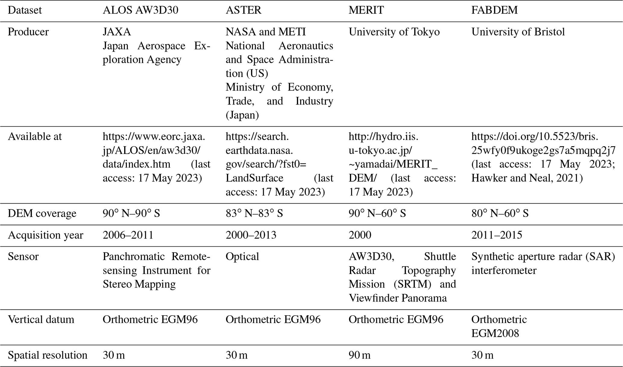
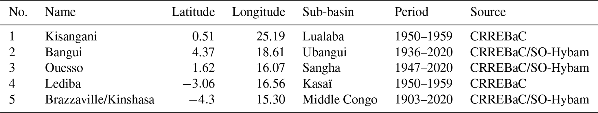
Table 2 Locations and main characteristics of the in situ discharge stations used in this study. The number in the first column refers to the location of the station in Fig. 1.

3.3 Digital elevation model

We used four freely available global digital elevation models (DEMs) (Table 1): (1) ASTER version 3, (2) the Advanced Land Observing Satellite (ALOS), (3) Multi-Error-Removed Improved Terrain (MERIT), and (4) the Forest And Buildings removed Copernicus DEM (FABDEM).

DEMs are divided broadly into two categories based on the specific topographic surfaces they represent, which are digital surface model (DSM) and digital terrain model (DTM). DSM refers to the upper surface of natural and built or artificial features of the environment such as buildings, artificial features, and trees, while DTM represents the elevation of the Earth's surface with all natural and built features removed, i.e. the bare Earth surface (Guth et al., 2021; Hawker et al., 2022). Among the DEMs used, ASTER and ALOS are classified as DSMs. MERIT is closer to a DTM because of the removal of tree height bias, but it is not a complete DTM (Yamazaki et al., 2017; Hawker et al., 2022) due to other artifacts such as artificial features. In this study, only FABDEM can be considered a DTM (Hawker et al., 2022).

Therefore, in order to remove the presence of tree bias in DSMs, we subtract from them the forest canopy height from a global dataset (Potapov et al., 2020). For that, the global canopy height dataset, ASTER, and ALOS were all resampled to 90 m spatial resolution using the nearest-neighbour resampling method.

3.4 Global forest canopy height

The global forest canopy height (available at https://glad.umd.edu/dataset/gedi/, last access: 17 May 2023) is a global dataset developed by combining the Global Ecosystem Dynamics Investigation (GEDI) lidar forest structure measurement and Landsat analysis-ready data time series (Potapov et al., 2020). GEDI is a new spaceborne lidar instrument on board the International Space Station collecting data on the vegetation structure since April 2019 (Dubayah et al., 2020). The spatial resolution of the dataset is 30 m, providing the global forest canopy height map for the year 2019 in the WGS84 reference system. The dataset covers zones between 54^∘ N and 52^∘ S globally, and then we use it over the CRB. For more details on the dataset, we refer the reader to Potapov et al. (2020).

3.5 Lake water storage anomaly

Over the largest lakes of the CRB, time series of the monthly water storage anomaly for Lakes Bangweulu, Kivu, Mweru, Tanganyika, and Upemba (see Fig. 1 for their locations and Fig. S2 for their time series) are estimated using surface water extent and water level time series obtained from the HydroSat database (accessible at https://www.gis.uni-stuttgart.de/en/, last access: 17 May 2023; Tourian et al., 2022). After collecting the simultaneous lake water area and height measurements, the empirical relationship between lake surface water level and area is developed. This model represents the bathymetry of the lake for the part which is captured by remote-sensing observations. By assuming that the lake has a regular morphology and a pyramid shape between two consecutive measurement epochs, the lake water level area storage model is developed. Finally, time series of the lake water storage anomaly are calculated using the developed model and lake water level or surface extent measurements.

3.6 Auxiliary data

3.6.1 In situ river discharge

We used the monthly time series of historical and contemporary observations of in situ river discharge located at the outlet of five sub-basins (see Fig. 1 for their locations and Table 2 for their characteristics) obtained from the Congo Basin Water Resources Research Center (CRREBaC, https://www.crrebac.org/, last access: 17 May 2023) and from the Environmental Observation and Research project (SO-HyBam, https://hybam.obs-mip.fr/fr/, last access: 17 May 2023).

3.6.2 Rainfall

We used precipitation estimates from Multi-Source Weighted-Ensemble Precipitation (MSWEP) Version 2.8 (V2.8). MSWEP is a global precipitation product with a spatial resolution of 0.1^∘ at 3-hourly temporal resolution (also available at the daily scale) covering the period from 1979 to the present in near real time. MSWEP estimates are derived by optimally merging multiple precipitation data sources, such as gauge, satellite, and reanalysis estimates (Beck et al., 2019a). The latest MSWEP version (V2.8) includes several changes compared to its previous version (V2.2). Among the major updates, in addition to near-real-time (NRT) estimates, it also features new data sources that were defined based on their superior performances.

The historical MSWEP V2.8 considers (i) one model-based precipitation product, the European Centre for Medium-Range Weather Forecasts (ECMWF) ReAnalysis 5 (ERA5), (ii) two satellite-based precipitation products, the Integrated Multi-satellitE Retrievals for GPM (IMERG) algorithm and the Gridded Satellite (GridSat) data, and (iii) gauge observations from various sources: the Global Historical Climatology Network-Daily (GHCN-D), the Global Summary of the Day (GSOD) databases, and several national databases. On the other hand, MSWEP V2.8 NRT merges (i) two model-based precipitation products, ERA5 and National Centers for Environmental Prediction (NCEP) Global Data Assimilation System (GDAS) analysis and (ii) two satellite-based precipitation products, Global Satellite Mapping of Precipitation (GSMaP) and IMERG. MSWEP was globally and regionally assessed, and it exhibits realistic spatial precipitation patterns in frequency, magnitude, and mean (Beck et al., 2017, 2019b). MSWEP V2.8 is available via http://www.gloh2o.org (last access: 17 May 2023).

3.6.3 Total water storage anomaly from the Gravity Recovery and Climate Experiment mission

GRACE is a joint NASA and German Aerospace Center (DLR) mission launched in March 2002 (Tapley et al., 2004) and, together with its successor GRACE Follow-On (GRACE-FO) launched in 2018 (Tapley et al., 2019), provides estimates of changes in water storage at the basin scale. For the analysis in this study, we used data from GRACE and GRACE-FO Mascon data available at http://grace.jpl.nasa.gov (last access: 17 May 2023; Wiese et al., 2016, 2018). The mascon data provide surface mass changes with a spatial sampling of 0.5^∘ in both latitude and longitude (Watkins et al., 2015). From this dataset, we obtained time series of the terrestrial water storage anomaly (TWSA) over the CRB through area-weighted aggregation of those grid cells in basins.

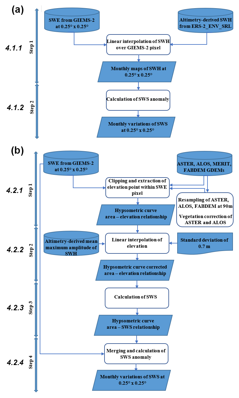
Figure 2 Schematic representation of (a) the multi-satellite and (b) hypsometric curve approaches' algorithms. The numbers on the left refer to the sections where the different steps are described.

4 Methods

In order to estimate SWS variations over the CRB, two approaches are used (Fig. 2): (a) the multi-satellite approach following the methodology of Frappart et al. (2008, 2011) and (b) the hypsometric curve approach following the methodology of Papa et al. (2013) and Salameh et al. (2017).

4.1 Multi-satellite approach

The multi-satellite approach (Fig. 2a) consists of the combination of the SWE and satellite-derived SWH over inland water bodies (rivers, lakes, reservoirs, wetlands, and floodplains), generally derived from radar altimetry over a common period of availability for both datasets (Frappart et al., 2008, 2011; Becker et al., 2018; Papa and Frappart, 2021). Therefore, this complementarity of multi-satellite observations offers the possibility of quantifying SWS changes and water volume variations in a watershed. SWE and SWH used in this study are respectively from GIEMS-2 and the family of spaceborne radar altimeters with a 35 d repeat cycle (hereafter ERS-2, ENV, and SRL). Their common period of availability is 1995–2015.

We summarize in the next sections the two-step methodology and, for more details, we refer the reader to Frappart et al. (2008, 2011, 2012, 2019).

4.1.1 Monthly maps of surface water level anomalies

Monthly maps of water level anomalies of 0.25^∘ spatial resolution referenced to the EGM2008 geoid are derived by combining GIEMS-2 and the combined long-term time series of ERS-2_ENV_SRL (1995–2015) satellite-derived water levels. For each given month of the water levels, these are linearly interpolated over the GIEMS-2 grid, and the elevation of each pixel is provided with reference to a map of minimum surface water levels estimated over 1995–2015 using the principle of the hypsometric curve approach between SWH from radar altimetry and SWE from GIEMS-2 to take into account the difference in altitude in each cell area of GIEMS-2 (see Frappart et al., 2012, for more details).

4.1.2 Monthly time series of surface water storage variations

Following Frappart et al. (2012, 2019), the time variations of SWS are computed at the basin scale as

$$\begin{array}{}\text{(1)}& \begin{array}{rl}{V}_{\mathrm{SW}}\left(t\right)& =R_{\mathrm{E}}^{\mathrm{2}}{\sum }_{j\mathit{ϵ}S}P({\mathit{\lambda }}_j,{\mathit{\phi }}_j,t)\left(h\right({\mathit{\lambda }}_j,{\mathit{\phi }}_j,t)\\ & -h_{\min }({\mathit{\lambda }}_j,{\mathit{\phi }}_j)\left)\cos \right({\mathit{\phi }}_j)\mathrm{\Delta }\mathit{\lambda }\mathrm{\Delta }\mathit{\phi },\end{array}\end{array}$$

where V_SW is the volume of surface water, R_E is the radius of the Earth (6378 km), P(λ_j, φ_j, t), $h({\mathit{\lambda }}_j,{\mathit{\phi }}_j,t)$, and h_min(λ_j,φ_j) are respectively the percentage of inundation, the water level at time t, and the minimum water level at the pixel (λ_j,φ_j), and Δλ and Δφ are respectively the grid steps in longitude and latitude.

The maximum error in the volume variation is estimated as follows:

$$\begin{array}{}\text{(2)}& \mathrm{\Delta }{V}_{\mathrm{SW},\max }\le \mathrm{\Delta }{S}_{\max }\mathit{\delta }{h}_{\max }+S_{\max }\mathrm{\Delta }\left(\mathit{\delta }{h}_{\max }\right),\end{array}$$

where ΔV_SW,max is the maximum error in the water monthly volume anomaly, S_max is the maximum monthly flooded surface, δh_max is the maximum water level variation between 2 consecutive months, ΔS_max is the maximum error for the flooded surface, and Δ (δh_max) is the maximum error for the water level between 2 consecutive months.

Note that the volume of SWS variations in a given basin is the sum of the contributions of the water storage contained in floodplains, wetlands, rivers, and small lakes. For larger lakes, as mentioned previously, estimates of SWS are complementarily obtained by the HydroSat database (Tourian et al., 2022). Therefore, the water storage analysis takes into account variations in floodplains, wetlands, rivers, and lakes.

4.2 Hypsometric curve approach using digital elevation models

In complement to the multi-satellite approach, we also used the hypsometric curve approach that consists of the combination of SWE and DEM-based topographic data. Following Papa et al. (2013), we summarize here the four-step process (Fig. 2b) to estimate SWS, using as an example the combination of GIEMS-2 SWE and FABDEM topography resampled at 90 m.

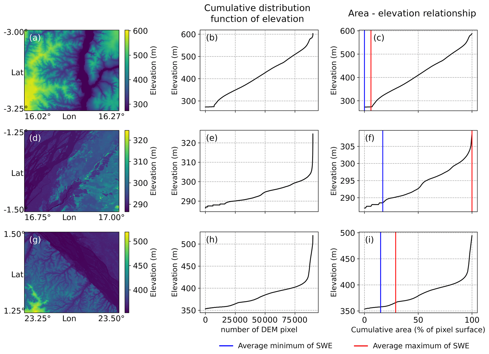
Figure 3 Hypsometric curve from FABDEM over the CRB. (a, d, g) Map of FABDEM elevations within a 773 km² pixel of GIEMS-2. (b, e, h) The hypsometric curve from FABDEM, i.e. the distribution of elevation values in each 773 km² pixel sorted in ascending order. (c, f, i) The hypsometric curve from FABDEM providing the relationship between the elevation and the inundated area of the 773 km² pixel (as a percentage). The blue (red) line is the average minimum (maximum) coverage of SWE observed by GIEMS-2 over 1992–2015.

4.2.1 Establishment of the hypsometric curve (area–elevation relationship)

For each GIEMS-2 pixel (Fig. 3; left column), we first derived the cumulative distribution function of elevation values within the corresponding FABDEM sub-set (Fig. 3; centre column). For each GIEMS-2 pixel, over the CRB, this corresponds to ∼95 000 elevation points falling within the satellite-derived SWE pixel, from which the hypsometric curve or the curve of cumulative frequencies is established. It is equivalent to the distribution of elevation values in each 773 km² pixel (with 773 km² of flood coverage at the abscissa converted into percentage 100 %) sorted in ascending order to represent an area–elevation relationship (Fig. 3; right column).

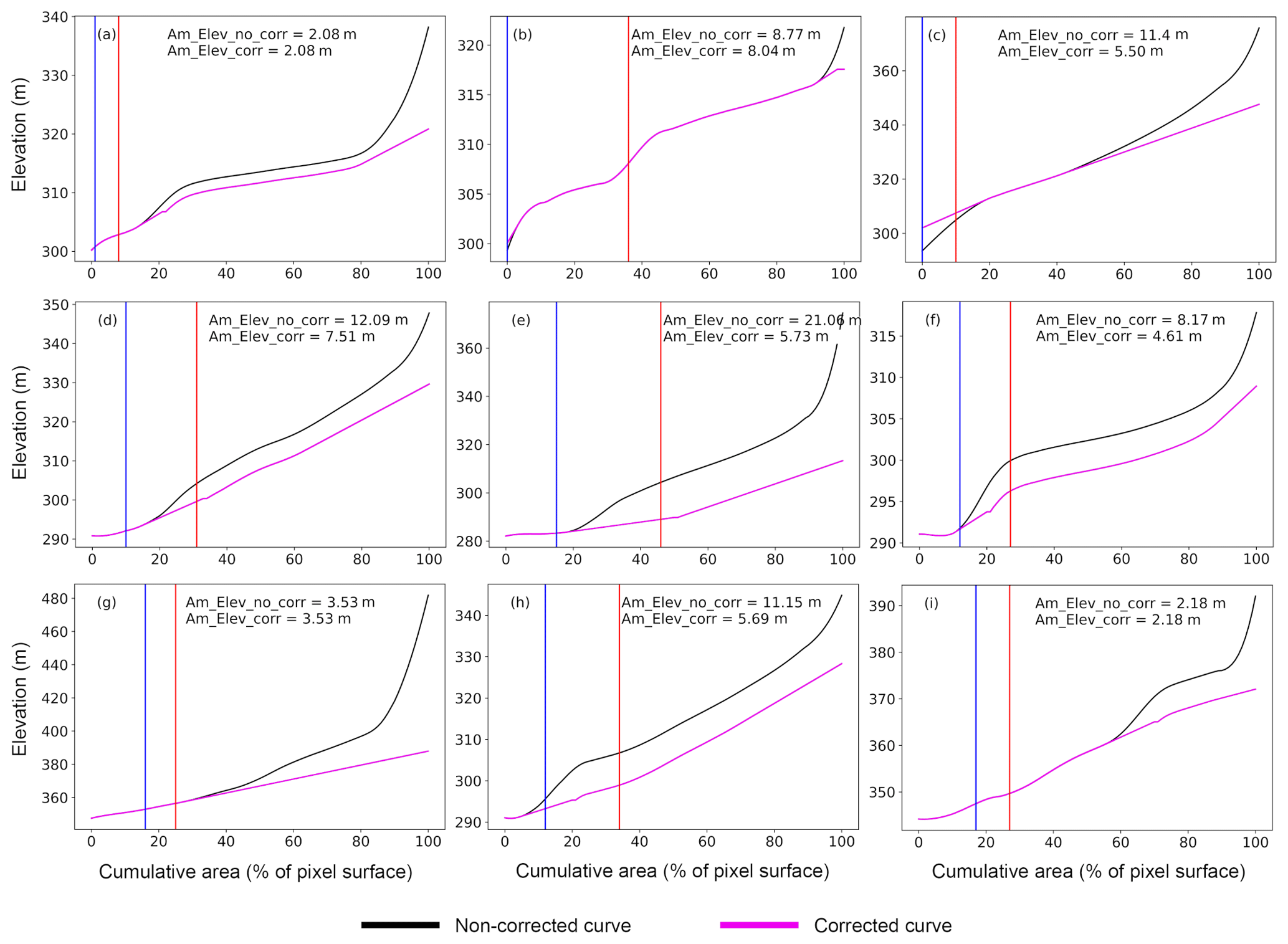
Figure 4 Correction of the hypsometric curve from FABDEM by calculating the SD (m) of elevation over 5 % flood coverage windows (see details of the procedure in Sect. 4.2.2). Black and magenta curves stand respectively for the non-corrected and corrected hypsometric curves. Am_Elev_no_corr (from the non-corrected curve) and Am_Elev_corr (from the corrected curve) are the elevation amplitude derived from the average minimum (blue line) and maximum (red line) coverage of surface water extent observed by GIEMS-2 over 1992–2015. Panels (a) to (i) show different pixels of GIEMS-2 in which the hypsometric curve is derived.

4.2.2 Correction of the hypsometric curve

To avoid the overestimation of SWS at the pixel level from the unrealistic amplitude, this step corrects the behaviour of the FABDEM hypsometric curve (Fig. 4). For each GIEMS-2 pixel, the established area–elevation relationship enables us to derive the elevation amplitude (i.e. similar to the amplitude of SWH) from the corresponding difference between the average annual minimum and the average annual maximum of SWE over the period 1992–2015. The mean maximum amplitude of SWH over the CRB varies between 1.5 and ∼7.5 m (see Fig. 5 of Kitambo et al., 2022a). In most cases (∼90 % of GIEMS-2 pixels), the elevation amplitude derived from the difference between the average minimum and maximum provides values that satisfactorily match the range of the SWH amplitude. Often, these realistic values correspond on the FABDEM hypsometric curve to the percentage of flood coverage representing the main channel or floodplains (lower part of the hypsometric curve) with a smooth increase in slope (as in Fig. 4a and g). However, Fig. 4 also points out that some elevation amplitudes (from ∼10 % of GIEMS-2 pixels) are above the range of 1.5 to ∼7.5 m. These pixels therefore present unrealistic amplitudes as compared to the range of previous findings over the CRB that can lead to the overestimation of SWS at the pixel level (Fig. 4c and d). Usually, these higher values are localized above 20 % of flood coverage.

For this, following Papa et al. (2013), we propose a simple procedure to correct the behaviour of the FABDEM hypsometric curve exceeding the range of 1.5 to ∼7.5 m in elevation amplitude. For each percent increment of flood coverage area, if the corresponding value of elevation belongs to a 5 % window of the 773 km² pixel (i.e. ∼35 km²) where the standard deviation (SD) of the elevation is below the 0.7 m threshold, the elevation value is kept. Conversely, if the elevation value corresponding to the percent increment of flood coverage belongs to a window in which the SD is above 0.7 m, the elevation value is replaced by the fitted value based on a simple linear regression analysis using the two previous elevation values of the hypsometric curve. For instance, a given elevation value corresponding to 8 % of flood coverage belonging to a window with an SD (i.e. calculated using values at 8 %, 9 %, 10 %, 11 %, and 12 %) greater than 0.7 m will be replaced by the fitted value calculated using the simple linear regression equation obtained from the values at 6 % and 7 %. The next SD will be computed with values of elevation at 9 %, 10 %, 11 %, 12 %, 13 %, and so on.

Several attempts at correction with different SD values ranging from 0.3 to 1.1 m were made (as shown in Fig. S3), and the SD of 0.7 m was chosen due to the realistic comparisons with the variations of surface water heights from an altimetric VS. This value is also in agreement with the one chosen for the Amazon River basin (Papa et al., 2013).

Note that there is a non-significant percentage of pixels (∼ 1 %) for which the hypsometric curve correction results in a slight increase in elevation amplitudes instead of a decrease (Fig. S4). However, these pixels generally provide acceptable estimates of SWS without unrealistic overestimations.

Note also that, in addition to this correction, the hypsometric curve obtained from ASTER and ALOS showed roughness in their curve (Fig. S5), which was smoothed out using the Savitzky–Golay filter embedded in the SciPy application programming interface (API) package in Python before applying the correction described above.

4.2.3 Establishment of the area–surface water storage relationship

The hypsometric curve representing the area–elevation relationship is then converted into an area–SWS relationship by estimating the surface water storage associated with an increase in the pixel-fractional open-water coverage (with an increment of 1 %) by filling the hypsometric curve from its base level to an upward level. Here we used three formulas for comparison purposes:

$$\begin{array}{}\text{(3)}& {\displaystyle }V\left(\mathit{\alpha }\right)={\sum }_{i=\mathrm{1}}^{\mathit{\alpha }}\left(H_i-H_{i-\mathrm{1}}\right)\cdot S_i,\text{(4)}& {\displaystyle }V\left(\mathit{\alpha }\right)={\sum }_{i=\mathrm{1}}^{\mathit{\alpha }}\left(H_i-H_{i-\mathrm{1}}\right)\cdot {\displaystyle \frac{S_i+S_{i-\mathrm{1}}}{\mathrm{2}}},\text{(5)}& {\displaystyle }V\left(\mathit{\alpha }\right)={\sum }_{i=\mathrm{1}}^{\mathit{\alpha }}{\displaystyle \frac{\left(H_i-H_{i-\mathrm{1}}\right)}{\mathrm{3}}}\cdot (S_i+S_{i-\mathrm{1}}+\sqrt{S_i\cdot S_{i-\mathrm{1}}}),\end{array}$$

where V is the surface water storage in cubic kilometres for a percentage of flood inundation α. Note that the increment is on a step of 1 %. S is the 773 km² area of the GIEMS-2 pixel, and H represents the elevation in kilometres for a percentage of flood inundation α given by the hypsometric curve.

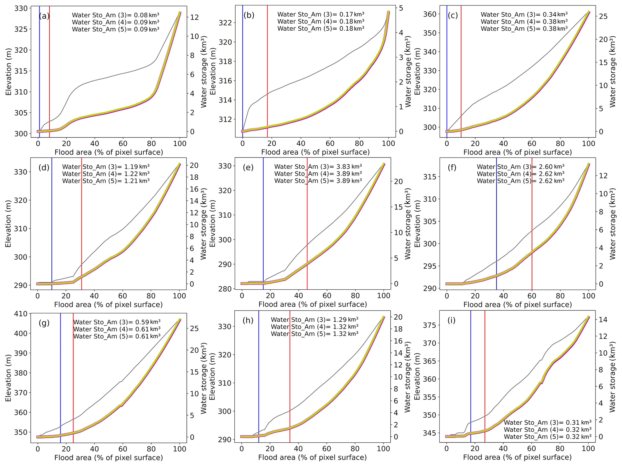
Figure 5 For the same GIEMS-2 pixel as in Fig. 3, the surface water storage profile, i.e. the relationship between SWS within each GIEMS-2 pixel and the fractional inundated area of 773 km² in percentage (abscissa – right ordinate) obtained from the area–elevation relationship (abscissa – left ordinate). Magenta, green, and orange colours are respectively the curve of SWS from Eqs. (3), (4), and (5). The grey curve stands for the corrected FABDEM hypsometric curve. The blue (red) line is the average minimum (maximum) coverage of surface water extent observed by GIEMS-2 over 1992–2015. Panels (a) to (i) represent different pixels of GIEMS-2 in which the hypsometric curve is derived.

Equations (3), (4), and (5) used to retrieve the estimation of SWS from the hypsometric curve approach are compared in Fig. 5. This shows that there is a slight difference in the SWS changes of about one-hundredth after the decimal point between the three Eqs. (3), (4), and (5) except for Fig. 5d and g, where the difference is one-tenth after the decimal point. Overall, the difference seems negligible, and we decided to use only Eq. (5) representing a volume of a trunk or a regular truncated pyramid for SWS computation based on the hypsometric curve approach.

4.2.4 Monthly time series of surface water storage variations

Finally, the hypsometric curve of the area–SWS relationship is combined with the monthly variations of SWE from GIEMS-2. This thus enables the estimation of SWS for each month by intersecting the hypsometric curve value with the GIEMS-2 estimates of pixel coverage for that month (Fig. 5). Note that, with such a method, the lowest level of storage refers to the level zero, determined by the minimum of SWE from GIEMS-2 observations for each pixel, from which the variation of the storage is started to be accounted for. Thus, the estimated SWS represents the increment above the minimum storage.

It is worth noting that, in the attempt at determining the extreme low storage values of exceptional drought years, this can be a potential source of uncertainties in the sense that the DEM's values should have produced credible elevation data for those periods at the lower part of the hypsometric curve. Such information is unfortunately difficult to assess.

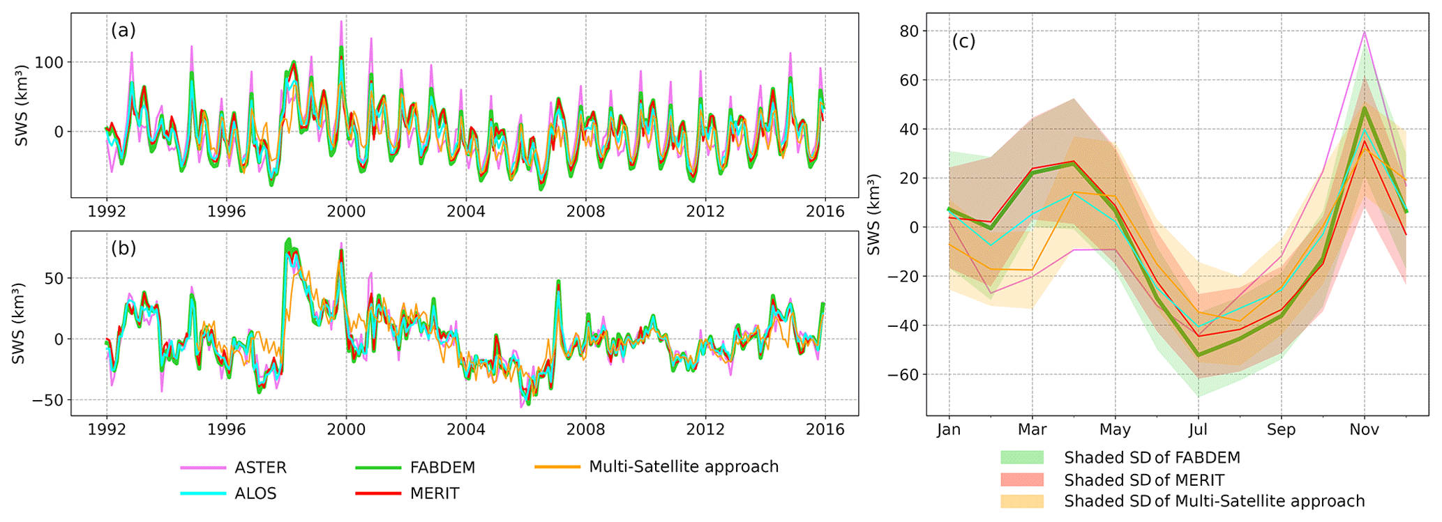
Figure 6 Long-term monthly time series of the Congo River basin's surface water storage (a) and its deseasonalized anomaly (b) obtained from the hypsometric curve approach for 1992–2015 (violet for ASTER, aqua for ALOS, lime green for FABDEM, red for MERIT) and from the multi-satellite approach for 1995–2015 (orange). (c) Annual cycles for each SWS estimate, with the shaded areas illustrating the standard deviations around their long-term mean.

5 Results and validation

5.1 Distribution and variability of surface water storage across the Congo River basin

Figure 6 presents the characteristics of the SWS temporal dynamics at the CRB scale (anomaly time series vs. its long-term mean, deseasonalized anomaly, and annual cycle for SWS aggregated for the entire CRB). It shows all SWS estimates computed with both the multi-satellite (for 1995–2015) and hypsometric curve (for 1992–2015) approaches from the use of the four DEMs (ALOS, ASTER, MERIT, and FABDEM).

Figure 6a shows, for the very first time, the long-term month-to-month variations of the CRB's SWS over a period of 24 years. It shows a strong seasonal cycle of SWS over the CRB with comparable behaviour in the peak-to-peak SWS variations from both approaches. The SWS amplitude ranges from ∼50 to ∼150 km³ over the years, showing a large year-to-year variability. The bimodal patterns that characterize the hydrological regime of the CRB (Kitambo et al., 2022a), linked to the variability of the Intertropical Convergence Zone (Kitambo et al., 2022a), are well depicted in the SWS estimates.

All SWS estimates from the different DEMs show fair agreement in their variations between them (Fig. 6a). However, we observed that SWS from ASTER (violet colour) tends to overestimate the SWS at the first peak (i.e. spanning over August–February) along the time series.

Figure 6b displays the deseasonalized anomaly (obtained by subtracting the mean monthly values over the considered periods 1992–2015 or 1995–2015 from individual months) of the CRB's SWS. A similar observation of the matching of the SWS anomaly from different approaches and DEM products is observed.

These SWS estimates also show a substantial interannual variability at the basin scale, especially in terms of annual maximum and minimum, pointing out extreme events in terms of droughts and floods that recently affected the CRB. Figure 6b reveals interesting and strong anomaly signals, such as the large positive peaks observed in 1997–1998 and 2006–2007. These can be related to the positive Indian Ocean Dipole (pIOD) events in combination with the El Niño events occurring in 1997–1998 and 2006–2007 that triggered floods in the western Indian Ocean and eastern Africa (Mcphaden, 2002; Ummenhofer et al., 2009; Becker et al., 2018; Kitambo et al., 2022a). Another major event is the severe drought that occurred in 2005–2006, which is clearly depicted in the CRB's SWS time series anomaly as the minima of the record (Fig. 6b). This is in agreement with Ndehedehe et al. (2019), Ndehedehe and Agutu (2022) and Tshimanga et al. (2022), who reported that, in the 1990s and 2000s, multi-year droughts in the CRB affected a significant part of the Congo basin. This interannual variability is also superimposed on variations at a larger timescale, from a few years to decades, such as a large increase in the SWS anomaly in 1996–1997 followed by a slight decrease until the minimum that occurred in 2005–2006, before SWS starts to slowly increase again after the 2007 peak until 2015.

Table 3 Mean annual amplitude over the CRB calculated from the multi-satellite and hypsometric curve approaches. Error statistics comparing SWS from ALOS, ASTER, and MERIT and the multi-satellite approach against SWS from FABDEM are considered here as the reference. Comparisons are done over the same period by aggregating all SWS pixels over the basin for the compared datasets. MAE stands for mean absolute error and RMSE for root-mean-squared error (km³).

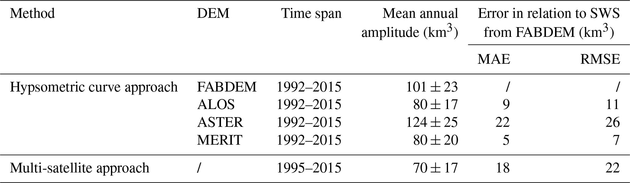
Figure 6c shows the CRB's SWS annual cycle (computed over the 1992–2015 and 1995–2015 periods for the hypsometric and multi-satellite approaches respectively), revealing a strong seasonal variation. Both approaches present a mean annual amplitude of the same order of magnitude (Table 3), with estimates ranging around 80±17, 101±23, 80±20 km³ (from ALOS, FABDEM, and MERIT respectively based on the hypsometric curve approach), and 70±17 km³ from the multi-satellite approach. These estimates are of the same order of magnitude as previous findings over the CRB, i.e. 81±24 km³ as in Becker et al. (2018). As a matter of comparison, the mean annual amplitude of SWS from ASTER represents ∼11 % of the Amazon basin's SWS mean annual amplitude of ∼1200 km³, as reported in Papa et al. (2013), Papa and Frappart (2021).

As observed in Fig. 6a, ASTER's SWS provides larger estimates, with a mean annual amplitude of $\sim \mathrm{124}\pm \mathrm{25}$ km³ (Table 3). This can be explained by the fact that, among the four DEMs (ALOS, ASTER, FABDEM, and MERIT), ASTER has a greater vertical error (i.e. 17 m; see Table 1 of Hawker et al., 2019) compared to the others and, consequently, this can impact the elevation amplitude (derived at step 2 of Sect. 4.2 used to calculate the SWS variations (step 3 of Sect. 4.2).

Table 3 also presents the statistical errors comparing FABDEM's SWS dataset to other estimates and reinforces the difference highlighted in SWS magnitude between different approaches and DEMs. Note that trees and urban-area biases are only removed from FABDEM, and thus it seems to be the most adequate DEM in representing hydrology processes (Hawker et al., 2022). ALOS and MERIT have provided small errors, as reflected in the mean absolute error (MAE) (9 and 5 km³) and the root-mean-squared-error (RMSE) values (11 and 7 km³) compared to values greater than 15 km³ of MAE and above 20 km³ of the RMSE from the multi-satellite approach and the ASTER DEM.

At the basin scale, Fig. 6c clearly depicts a double peak, with a SWS maximum reached in November for the first peak and in April for the second peak. In comparison with the annual cycle of the GIEMS-2 SWE (Fig. 7c of Kitambo et al., 2022a), the first peak of the SWS maximum is in phase with the maximum SWE, while for the second peak there is a 1-month delay, with the maximum SWE occurring in March. This can be explained by the non-linear relationship between SWE and SWS through the hypsometric curve approach.

It is important to note that the SWS from FABDEM and MERIT shows a very good fit in all the seasons, whereas ALOS slightly underestimates the storage at the second peak. In contrast to the others, ASTER shows peculiar behaviour, with its SWS largely underestimating and overestimating the storage at the second and first peaks respectively of the hydrological regime.

In agreement with the results from the SWS hypsometric curve approach, the SWS from the multi-satellite approach also points out the maximum SWS in November and April for the first and second peaks. However, the dynamics of the SWS from the multi-satellite approach differ from the others over the period from February to May. Over that period of time, the hydrological regime of the basin is more controlled by the south-eastern region, especially by the Lake Bangweulu and Lake Upemba area (Kitambo et al., 2022a). In this region, the spatial distribution of VSs is not sufficient enough (Fig. S1) to obtain a very accurate representation of the temporal variations of the SWS even if the mean annual cycle variations of some VSs from ENV and SRL were used to account for the water level over the entire 1995–2015 period. This might explain in part the different dynamics observed in the SWS variations over February–May in the south-eastern region.

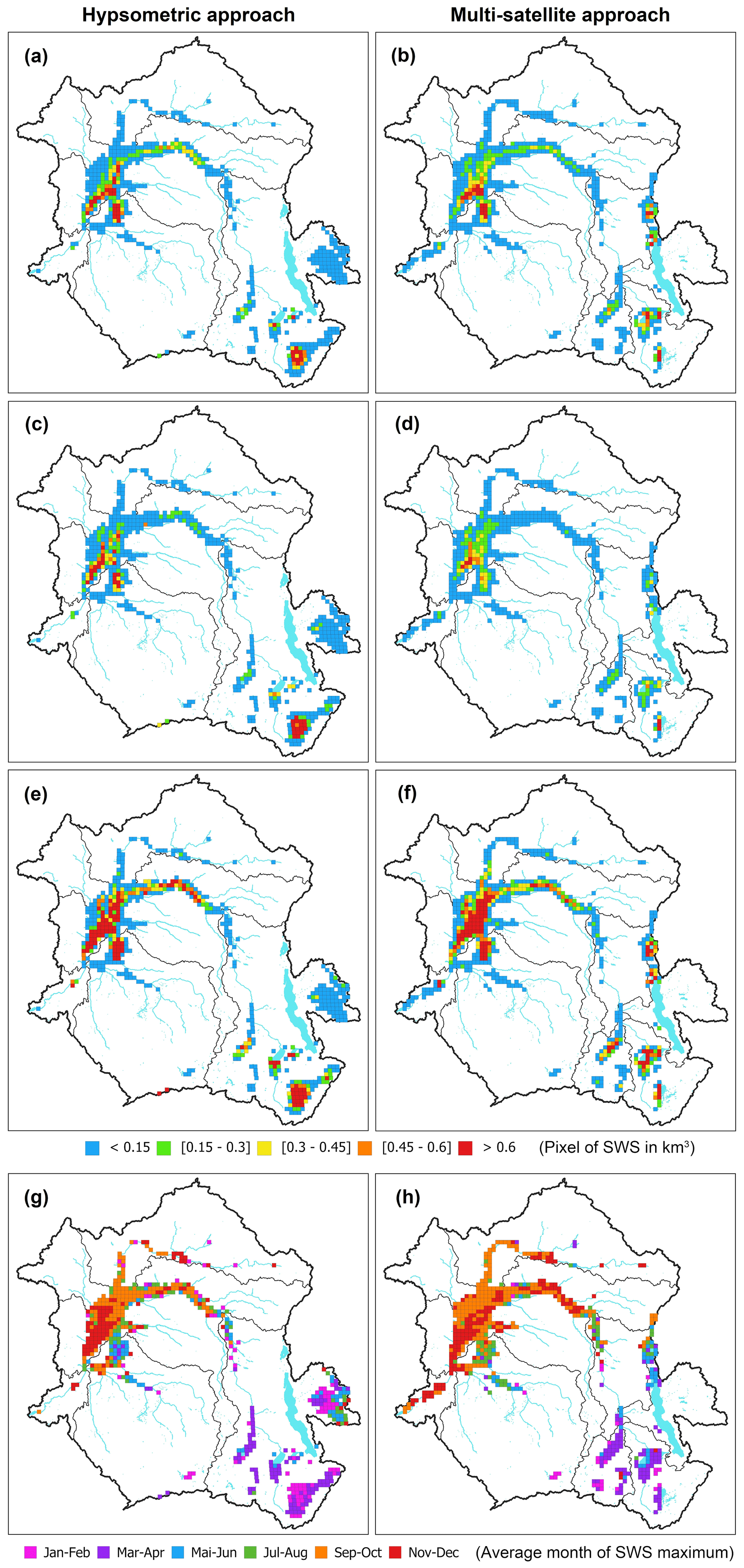
Figure 7 Spatial characterization of the CRB's SWS variations from the FABDEM hypsometric curve approach (over 1992–2015, a, c, e, g) and from the multi-satellite approach (over 1995–2015, b, d, f, h). (a, b) SWS mean annual amplitude (km³). (c, d) SD (km³). (e, f) Mean annual maximum (km³) and (g, h) average month of the maximum (months).

In parallel to Fig. 6, Fig. 7 presents the spatial distribution of SWS dynamics (mean annual, SD, mean annual maximum, and the average month of the maximum) for the entire CRB. In the following parts of the paper, the estimates obtained with the FABDEM DEM will become our reference, and we will use them to display the results. This is justified by FABDEM DEM topographic characteristics and properties, which makes it the closest to a DTM. The estimates obtained with the other DEM will be displayed in the Supplement (Fig. S6).

In agreement with the spatial distribution of SWE across the CRB (Fig. 6 of Kitambo et al., 2022a), SWS (Fig. 7a and b) shows realistic spatial patterns along the Congo River and the Cuvette Centrale and depicts quite well the other main structures of the basin, for instance the main tributaries (e.g. the Sangha, Ubangui, Luvua, Luapula, and Lualaba rivers) along with their large wetlands and floodplains. These are characterized by a strong variability in SWS (Fig. 7c and d).

Higher values of SWS ranging from 0.3 to 0.6 km³ in a 773 km² pixel dominate the extensive wetlands and floodplains such as the Cuvette Centrale and in the south-eastern part of the basin (the Upemba and Bangweulu region). These regions display a large variability as well (in terms of the SD, Fig. 7c and d) and are characterized by maximum values of surface water storage generally greater than 0.6 km³ per 773 km² pixel (Fig. 7e and f).

The heart of the Cuvette Centrale, Lake Mai-Ndombe (in the Kasaï sub-basin), and a large part of the main channel of the Congo (up to the Lomami River) presents the maximum values of the SWS change in the basin. The same observation is made for the lakes in the Upemba depression (e.g. Lake Upemba), Mweru, and Bangweulu. These maximum values are reached in September–October in the upper part of the Cuvette Centrale and November–December in its lower part (Fig. 7g and h). In the Lualaba sub-basin, the average month of the maximum of SWS is January–February, while in the other parts, such as Lake Mweru and the eastern part of Lake Bangweulu, with its large grassy swamps and floodplains, it recorded in March–April. Conversely to the general trend in the Cuvette Centrale, the regions of Lake Tumba and Lake Mai-Ndombe reached their maximum SWS in July–August.

In general, the results from the hypsometric curve (Fig. 7, left column) and multi-satellite (Fig. 7, right column) approaches are quite similar in terms of spatial distribution for both the magnitude and variability of the changes. Nevertheless, as expected, the multi-satellite dataset approach shows a limitation in terms of spatial distribution caused by the reduced availability of the combined long-term VSs in some regions. For instance, there is a lack of observations of the eastern part of Lake Tanganyika and in the Bangweulu region, where the spatial distribution of SWS from the multi-satellite approach is smaller than that of the FABDEM hypsometric curve approach. This is mainly explained by the sparse availability of long-term satellite-derived (ERS-2–ENV–SRL) time series in that region, leading to less distributed SWS estimates in these regions.

On the other hand, SWS variations from the hypsometric curve approach also present limitations, mainly on small lakes and around large lakes, where there are almost no variations in elevation from the DEMs, leading to flat hypsometric curves and therefore to the computed storage having zero changes. This is for instance the case around Lake Kivu in the Lualaba sub-basin. In this case, the SWS change in the lake is then added to the dataset using the lake water storage anomaly computed independently (see the data description in Sect. 3.5).

Finally, for comparison purposes, Fig. S6 shows the same analysis in terms of spatial distribution and variability of SWS across the basin for the other estimates based on the hypsometric curve approach (i.e. ALOS; see Fig. S6, left column; ASTER; see Fig. S6, middle column; MERIT; see Fig. S6, right column). In general terms, results are consistent between one another. The pattern of SWS in terms of the distribution and order of magnitude of the mean annual (Fig. S6a, b, and c), variability in terms of the SD (Fig. S6d, e, and f), mean annual maximum (Fig. S6g, h, and i), and average month of the maximum (Fig. S6j, k, and l) between the three DEMs and FABDEM are generally similar, although results from the ASTER DEM (Fig. S6b, e, and h) underestimate the storage (i.e. values ranging between 0.15 and 0.45 km³) compared to other DEMs (i.e. values greater than 0.6 km³) in the Bangweulu–Upemba region (e.g. Lake Bangweulu, Lake Upemba).

At the sub-basin scale, the mean annual amplitude for the five sub-basins is provided as follows. The Middle Congo is the sub-basin with a large amplitude (71±15 km³) associated with the strong variations of the SWS anomaly observed in the Cuvette Centrale. It is followed by the Lualaba sub-basin with 59±15 km³ due to the presence of major lakes (Kivu, Tanganyika, Mweru, Bangweulu) and large wetlands that show large variability and that are characterized by maximum values of surface water storage generally greater than 0.6 km³ per 773 km² pixel. Sangha and Kasaï show quite similar annual amplitudes (i.e. 24±5 and 24±6 km³ respectively). Both sub-basins are overlapped at their mouth (i.e. the downstream part) by the Cuvette Centrale. Among the five sub-basins, Ubangui is the one with the smallest mean annual amplitude (13±4 km³), although it is among the two northern sub-basins (i.e. Ubangui and Sangha) with higher satellite-derived SWH mean maximum amplitude (see Fig. 5a of Kitambo et al., 2022a). As observed for the Sangha and Kasaï sub-basins, the Ubangui sub-basin is also occupied in its downstream part by the Cuvette Centrale (Fig. 1).

5.2 Evaluation against independent datasets

In order to evaluate the monthly estimates of the large-scale SWS over the CRB, we compare, at the basin and sub-basin levels, their seasonal and interannual variability against other independent hydrological variables such as precipitation data from MSWEP V2.8 and in situ discharges. For clarity purposes, only the SWS results from the hypsometric curve approach with FABDEM and from the multi-satellite approach are displayed and discussed here.

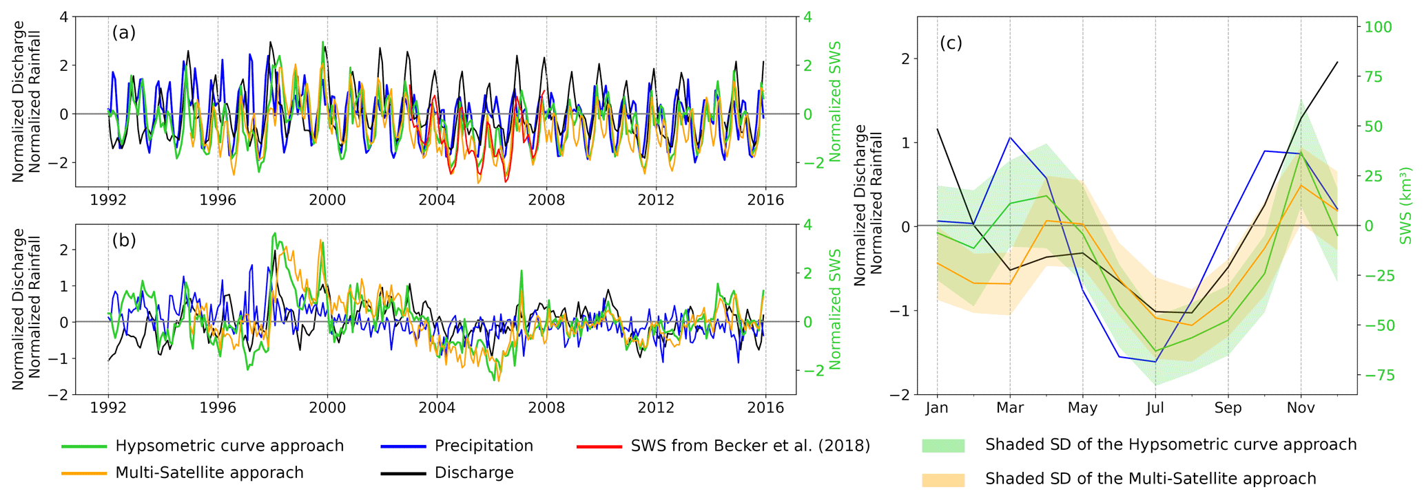
Figure 8 Comparison between the monthly aggregated normalized surface water storage anomaly, normalized precipitation anomaly over the basin and normalized discharge anomaly variations (at the outlet of the CRB, Brazzaville/Kinshasa station) (for comparison purposes, SWS, precipitation, and discharge were normalized by dividing their time series of anomalies by the standard deviation of the raw series). (a) For the entire Congo basin, the green and orange lines represent respectively the SWS anomaly variations from the hypsometric curve (over 1992–2015, from FABDEM) and multi-satellite (over 1995–2015) approaches, the red line shows the SWS anomaly estimated by Becker et al. (2018) over 2003–2007, the black line is the discharge, and the blue line is the normalized precipitation anomaly. (b) Deseasonalized normalized anomaly for SWS (green and orange), precipitation (blue), and discharge (black). (c) Normalized mean annual cycle for the three variables (except for the SWS), with the shaded areas depicting the standard deviations around the SWS anomaly.

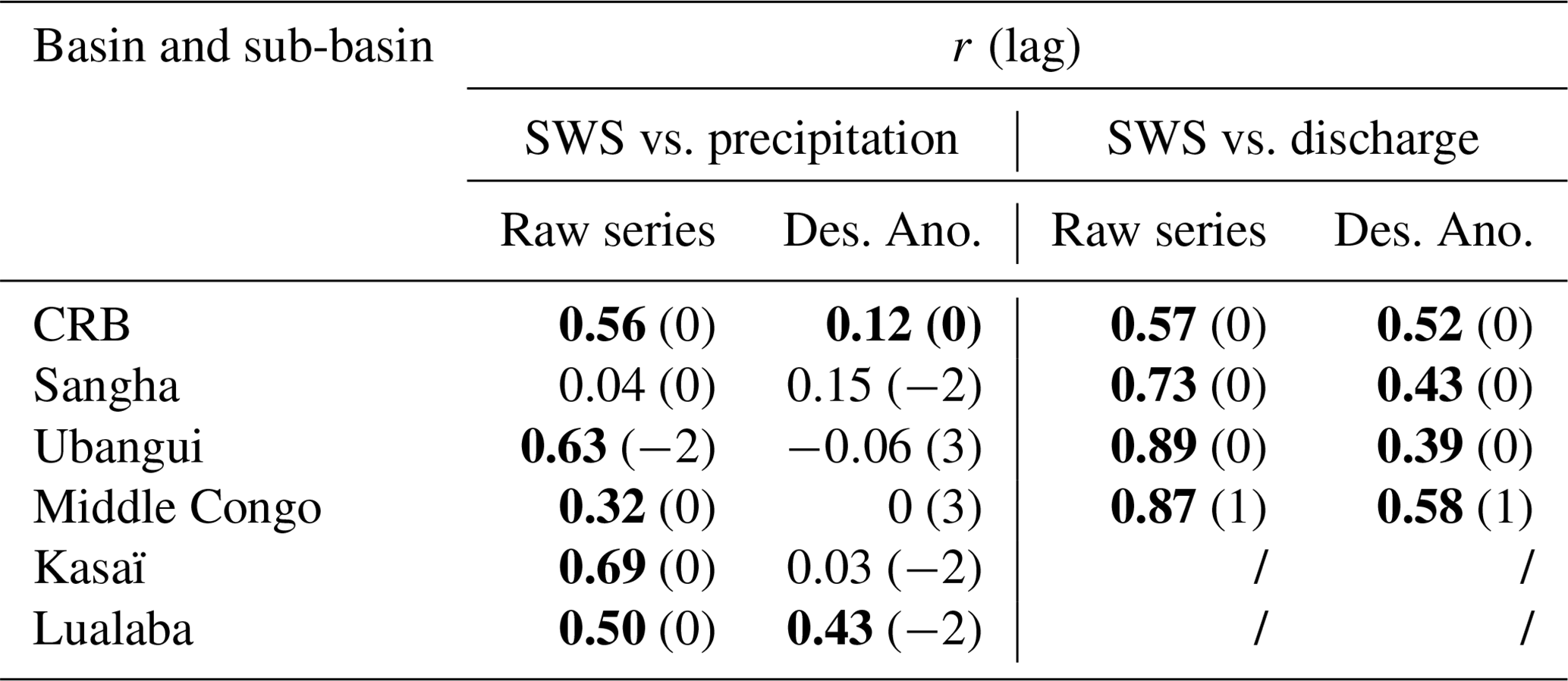
Table 4 Summary of the maximum linear Pearson correlation coefficient r along with the lag for the comparison between SWS, precipitation, and discharge. “Des. Ano.” stands for deseasonalized anomalies. In bold are shown the significant correlation coefficients with p value <0.01. For the Kasaï and Lualaba sub-basins, no contemporary discharge data are available, and therefore no correlations are reported.

At the basin level, Fig. 8 presents the comparison of the aggregated normalized SWS anomaly variation over the entire basin against the normalized precipitation anomaly and the in situ normalized discharge anomaly at the outlet of the basin (Brazzaville/Kinshasa station; see Table 2). The normalized anomalies here are estimated by subtracting the mean value of the time series from individual months and by dividing the obtained series by the SD of the original time series. As a complement, we report in Table 4 the maximum linear Pearson correlation coefficient along with its lag, calculated between the aggregated normalized SWS anomaly variation, the normalized precipitation anomaly, and the in situ normalized discharge anomaly at basin and sub-basin scales.

Figure 8a presents a fair agreement between the SWS and the other two hydrological variables, with a maximum correlation coefficient r of 0.56 (lag = 0; p value <0.01) between SWS and precipitation variations. A similar correlation coefficient (r=0.57 with a 0-month lag; p value <0.01) is found between the normalized SWS anomaly and the in situ normalized discharge anomaly. The deseasonalized normalized anomalies (acquired by subtracting the mean monthly values over the considered periods 1992–2015 or 1995–2015 from individual months and dividing by the SD of the raw series) (Fig. 8b) show correlation coefficients of r=0.52 (lag = 0; p value <0.01) and r=0.12 (lag = 0; p value <0.05) respectively between SWS vs. in situ discharge and SWS vs. precipitation.

Additionally, we also perform a comparison with previous estimates of SWS over the Congo basin from Becker et al. (2018), estimated using the multi-satellite approach and available over the period 2003–2007. The assessment with the SWS anomaly from FABDEM shows good agreement (Fig. 8a) with similar amplitude and a maximum correlation coefficient of r=0.73 (lag = 0; p value <0.01).

At the seasonal timescale, Fig. 8c reveals for the first peak (i.e. August–February) that the SWS anomaly reaches its maximum in November, 1 month before the maximum of the river's normalized discharge anomaly (December) and after the maximum of normalized precipitation anomaly data (October). The same observation is made in terms of the temporal shift for the second peak (i.e. March–July), where the maximum of the SWS anomaly occurs in April, 1 month later for the normalized discharge anomaly, and 1 month before for the normalized precipitation anomaly respectively in May and March.

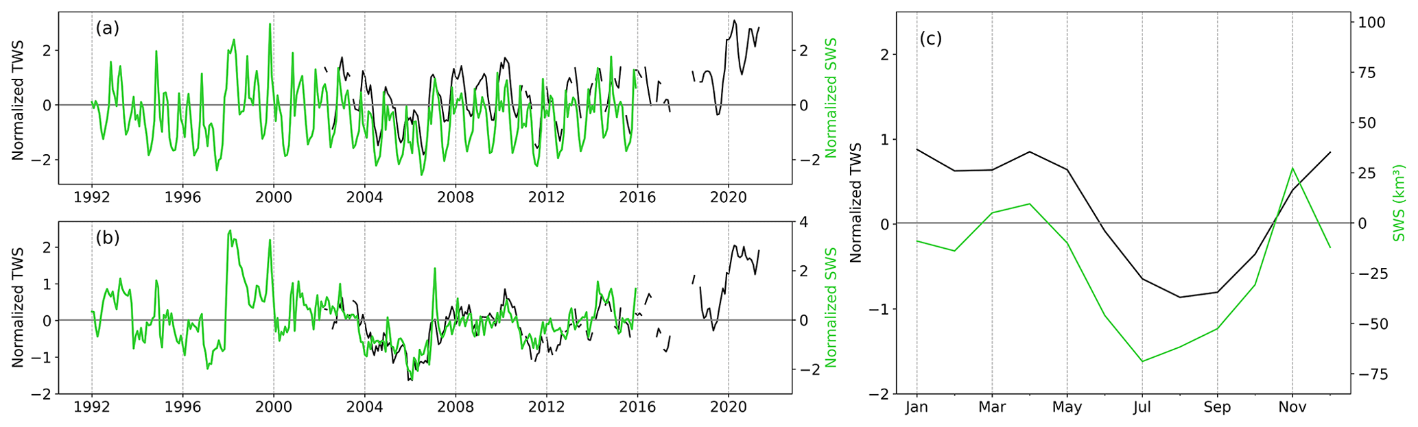
Figure 9 Comparison between the monthly aggregated normalized surface water storage anomaly and the normalized terrestrial water storage anomaly (TWSA) over the basin (for comparison purposes, SWS and TWSA were normalized by dividing their time series of anomalies by the standard deviation of the raw series). (a) For the entire Congo basin, the green and black lines represent respectively the SWS anomaly variations from the hypsometric curve approach (over 1992–2015, from FABDEM) and TWSA. (b) Deseasonalized normalized anomaly for SWS (green) and TWSA (black). (c) Normalized mean annual cycle for TWSA (black) (except for SWS, in green) calculated over the same period of data availability of the two variables, SWS and TWSA.

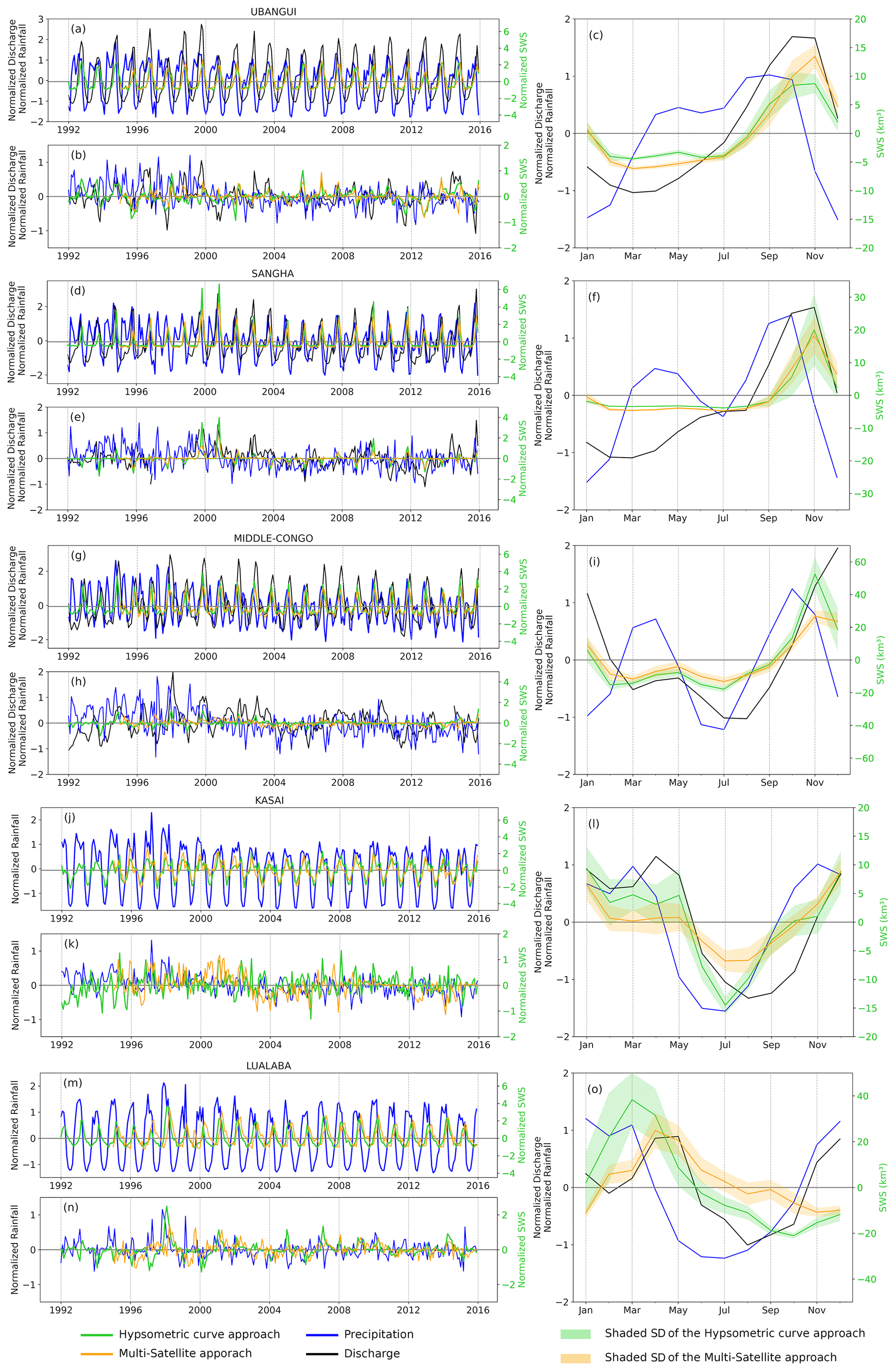
Figure 10 Same as Fig. 8, but the discharge is considered at the outlets of each sub-basin, and the precipitation is the estimated mean over each sub-basin; both are compared to the normalized SWS anomaly variations. (a) For each sub-basin, the green and orange lines represent respectively the SWS anomaly variations from the hypsometric curve (over 1992–2015, from FABDEM) and multi-satellite (over 1995–2015) approaches, the red line shows the SWS anomaly from Becker et al. (2018) over 2003–2007, the black line is the normalized discharge anomaly, and the blue line is the normalized precipitation anomaly. (b) Deseasonalized normalized anomaly for SWS (green and orange), precipitation (blue), and discharge (black). (c) Normalized mean annual cycle for the three variables (except for the SWS), with the shaded areas depicting the standard deviations around the SWS anomaly.

Figure 9 displays the comparison at the basin level between the aggregated normalized SWS anomaly and TWSA from GRACE. Both variables show a similar interannual variability during the common period of availability of data (i.e. 2002 to 2015), presenting a fair correlation of r=0.84 (lag = 1; p value <0.01; Fig. 9a). It is also worth mentioning that both datasets capture the bimodal patterns. Figure 9b presents the deseasonalized normalized anomaly for the two variables (r=0.4; lag = 0; p value <0.01), showing quite similar variations, especially in the long-term variability. We also notice the higher magnitude of the normalized SWS anomaly as compared to the normalized TWSA. At the seasonal timescale, Fig. 9c reveals a similar behaviour, with the two peaks depicted in the two variables, one in November–December and one in April. The lowest level of the SWS occurs in July, which is 1 month ahead of the TWSA minimum. Figure 10 presents the same comparison as done in Fig. 8 but at the sub-basin level (considering the Ubangui, Sangha, Middle Congo, Kasaï, and Lualaba sub-basins; see Fig. 1). The seasonal variations of all the sub-basins are provided in Fig. 10 (right column). The outlet of the Kasaï and Lualaba sub-basins provides historical observations (i.e. data before the 1990s), and thus the comparison with its in situ normalized discharge anomaly time series was integrated only at the annual cycle. For the Ubangui, Sangha, and Lualaba sub-basins, the maximum linear correlation coefficient is not significant between normalized SWS anomaly and normalized precipitation anomaly variations at the interannual level and their associated anomaly (Fig. 10a, b, d, e, m, and n, Table 4). This could be associated with the bimodal dynamics observed in the precipitation data, whereas the SWS variations do not show that behaviour. Becker et al. (2018), using similar datasets (GIEMS-1 for SWE and VS from ENVISAT), reported the same observation between precipitation data with bimodal patterns and SWE with unimodal patterns (Fig. 4 of Becker et al., 2018). Another reason could be that, for Ubangui and Sangha, SWS is mainly a function of discharge variations, while for the Lualaba sub-basin, which encompasses many lakes and floodplains, the various processes and their link for instance with evaporation lead to an insignificant precipitation–SWS correlation. Additionally, one can observe a negative lag between the normalized SWS anomaly and the normalized precipitation anomaly for the Ubangui and Lualaba sub-basins, which is not physically acceptable, since we expect a positive temporal shift between SWS and precipitation. This is probably due to the fact that SWS shows a unimodal pattern, while precipitation shows a bimodal pattern. Nevertheless, the comparison between the normalized SWS anomaly vs. the normalized discharge anomaly for Ubangui and Sangha, except for the Lualaba sub-basin, shows a fair correlation coefficient (r>0.7; p value <0.01) at the interannual timescale (Fig. 10a and d). Their related deseasonalized normalized anomalies (Fig. 10b and e) present lower values of correlation coefficients (r<0.4; p value <0.01). Regarding the Middle Congo and Kasaï sub-basins (Fig. 10g and j), the maximum linear correlation coefficients are r=0.32 and r=0.69 (lag = 0; p value <0.01) respectively between the normalized SWS anomaly and the normalized precipitation anomaly. Their associated deseasonalized normalized anomaly (Fig. 10h and k) does not show a significant correlation coefficient. In contrast to this, for the Middle Congo basin, the comparison between SWS and discharge provides a moderate correlation coefficient for both the interannual and deseasonalized anomaly variations (r>0.5 with a delay lag of 1 month; p value <0.01). In accordance with other results (see Fig. 10h of Kitambo et al., 2022a), the Middle Congo basin appears to be the main sub-basin for which the variability of the normalized discharge anomaly at the outlet Brazzaville/Kinshasa station is fairly related (∼35 %) to the variations of the normalized SWS anomaly in the Cuvette Centrale region due to its significant correlation coefficient of r=0.58 between the deseasonalized normalized anomaly of both SWS and discharge. The northern and Middle Congo sub-basins reach their SWS anomaly maximum in November (for Sangha and the Middle Congo, Fig. 9f and i) and October (for Ubangui, Fig. 10c), and this is in phase with the maximum of the normalized discharge anomaly and a backward temporal shift of 1 month with the normalized precipitation anomaly. Compared to northern sub-basins, southern sub-basins (Kasaï and Lualaba) for the period January to May reach their SWS anomaly maximum in March (Fig. 10l and o), which is in phase with the occurrence of the maximum of the normalized precipitation anomaly. The maximum of the normalized discharge anomaly occurs 2 months later in May for Lualaba and 1 month later for Kasaï. In contrast to the other sub-basins, Kasaï and the Middle Congo have depicted the bimodal patterns in SWS anomaly variations. For the Middle Congo, the first peak is reached in November and the second in May, while for Kasaï, the first peak occurs in December, and the second peak with a steady evolution occurs in March and May. Similar results were observed in the Cuvette Centrale by Frappart et al. (2021).

The temporal patterns in Figs. 8 and 10 follow alternatively wet and dry events associated with large-scale climatic phenomena for all the datasets (SWS, precipitation, and discharge). A focus on the Lualaba and Kasaï deseasonalized normalized anomalies of SWS reveals that there are two main sub-basins significantly impacted (large positive anomaly in Fig. 10k and n) by the major flood event triggered by the positive Indian Ocean Dipole in combination with the El Niño event that characterized the period 1997–1998. Conversely, recent studies using hydrometeorological datasets have shown that some parts of the CRB are subject to a long-term drying trend over the past decades (Hua et al., 2016; Ndehedehe et al., 2018). The droughts that affected large areas of the CRB in recent years are amongst the most severe ones in the past decades (Ndehedehe and Agutu, 2022), including the large anomalous event of the 2005–2006 drought (Fig. 8). This is further investigated below.

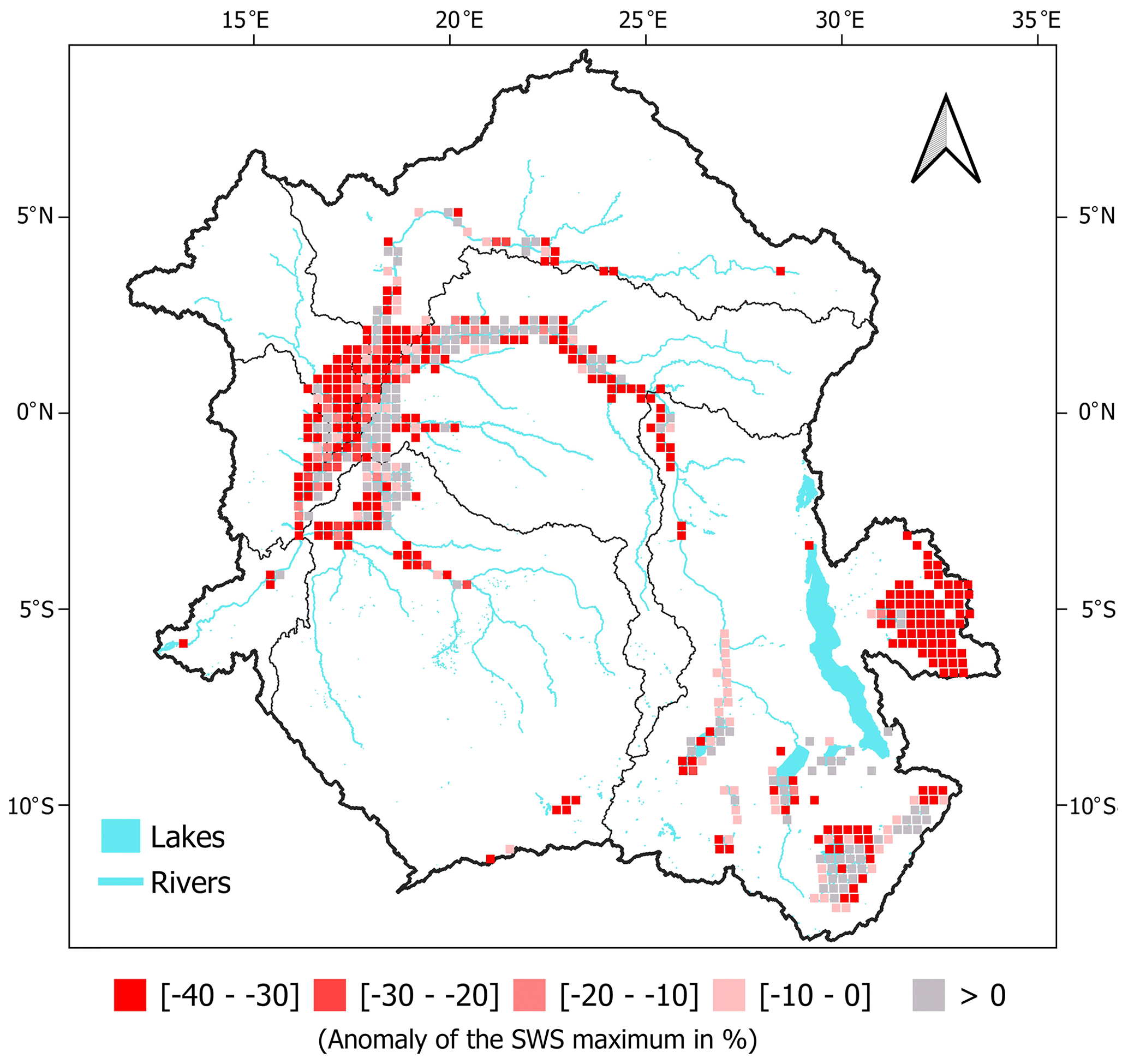
Figure 11 The 2005–2006 drought over the CRB as seen from the hypsometric curve approach SWS dataset based on FABDEM. Anomaly of the maximum SWS over November 2005 to January 2006 as compared to the 1992–2015 November–December–January mean value. The unit is in percentage of the 24-year mean monthly value.

6 Application: the spatio-temporal dynamics of SWS during the 2005–2006 drought

SWS estimates are essential in the characterization of large-scale, extreme-climate events such as droughts and floods (Frappart et al., 2012; Pervez and Henebry, 2015; Papa and Frappart, 2021). Here, we investigated the spatial signature and distribution of the major drought that occurred at the end of 2005 and in early 2006 across the CRB (Ndehedehe et al., 2019; Ndehedehe and Agutu, 2022). During that period, the SWS anomaly was at its lowest level at the basin scale (Fig. 6b). The spatial patterns of this drought are further illustrated in Fig. 11 using the FABDEM estimates. The anomaly of SWS from FABDEM at the end of 2005 and in early 2006 is estimated here by subtracting the November–December–January mean values over 1992–2015 from the maximum value between November 2005 and January 2006 and by dividing the obtained value by the November–December–January mean values.

Figure 11 shows that, during that period, the major part of the basin was affected by large negative anomalies of SWS, with values sometimes reaching a 50 % deficit as compared to their long-term average. This clearly shows a widespread severe drought across the basin ($<-\mathrm{40}$ % of the mean maximum), even if some parts of the Oubangui sub-basin and the Lukenie River in the north of the Kasaï sub-basin are relatively less affected ($>-\mathrm{10}$ % of the mean maximum of SWS). Figure 11 shows the large drought spatial signature of the south-eastern wetlands and floodplains (e.g. Bangwelo, Upemba) in the Lualaba sub-basin, with SWS estimated to be more than −40 % of the mean maximum during that period. Notably, the heart of the Cuvette Centrale displays a stronger negative signal in terms of SWS. The hydrological dynamic in the Cuvette Centrale might explain why the main stream receives water from all the adjacent wetlands and why streams experience a less intense impact of drought (Lee et al., 2011).

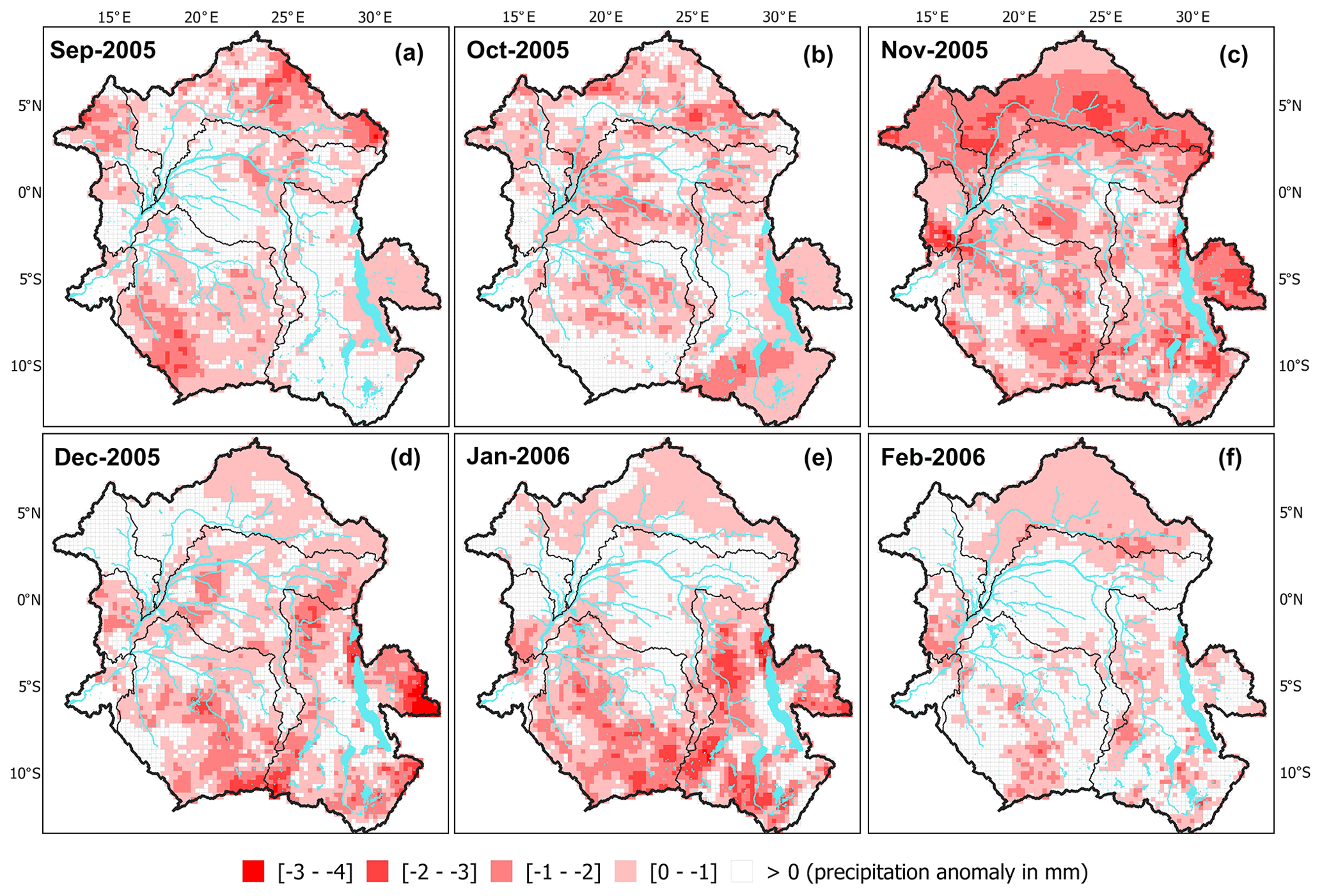
Figure 12 Monthly mean spatial distribution of the MSWEP precipitation anomaly in millimetres (resampled at 0.25^∘ spatial resolution) from the period September 2005 to February 2006 based on the 1992–2015 climatology.

This aligns with the previous findings that large parts of the CRB are found to be extensively affected (Ndehedehe et al., 2019), and this is confirmed by analysing the monthly mean spatial distribution of the MSWEP precipitation anomaly (Fig. 12) around that period of time. Figure 12 shows the monthly mean spatial distribution of the MSWEP precipitation anomaly at 0.25^∘ spatial resolution from the period September 2005 to February 2006 based on the 1992–2015 climatology. Over the 6 months, November 2005 to January 2006 are the most impacted months (Fig. 12c–e). November 2005 (Fig. 12c) displays a widespread negative anomaly all over the basin, whereas December 2005 (Fig. 12d) and January 2006 (Fig. 12e) show severe negative anomalies only in the southern part of the basin, in accordance with the spatial distribution of SWS across the basin as described previously. However, some parts of the Oubangui sub-basin and the Lukenie River in the north of the Kasaï sub-basin seem to be relatively less affected by the drought in terms of SWS, even if the large precipitation negative anomaly is observed in these regions. Investigating the climatic and hydrological drivers of these anomalous events in the CRB is far beyond the scope of the present study, but our results point to the capability of this new long-term estimate of SWS to be used in future studies.

7 Data availability

The SWS estimates from the multi-satellite approach (1995–2015), the hypsometric curve approach providing the surface water extent area–height relationships from the four DEMs (before and after the corrections), the surface water extent area–storage relationships, and the four SWS estimates (1992–2015) are publicly available for non-commercial use and are distributed via the following URL/DOI: https://doi.org/10.5281/zenodo.7299823 (Kitambo et al., 2022b).

8 Code availability

Here we provide the Python code to run the reproducibility of the hypsometric curve approach dataset of SWS. This code allows the application of the method elsewhere and is available at the Zenodo platform through the following URL/DOI link: https://doi.org/10.5281/zenodo.8011607 (Kitambo et al., 2023).

9 Conclusions and perspectives

In this study, we present an unprecedented dataset of the monthly SWS anomaly of wetlands, floodplains, rivers, and lakes over the entire Congo River basin during the 1992–2015 period at ∼0.25^∘ spatial resolution. Two methods are employed, one based on a multi-satellite approach and one on a hypsometric curve approach. The multi-satellite approach consists of the combination of SWE from GIEMS-2 and satellite-derived SWH from radar altimetry (long-term series ERS-2_ENV_SRL) on the same period of availability for the two datasets, here 1995–2015. The hypsometric curve approach consists of the combination of SWE from the GIEMS-2 dataset and hypsometric curves obtained from various DEMs (i.e. ASTER, ALOS, MERIT, and FABDEM). Both methods generate monthly spatio-temporal variations of SWS changes across the entire CRB, enabling for the first time the quantification of surface freshwater volume variations in the Congo River basin over a long-term period (24 years). The SWS computed from different approaches, multi-satellite and hypsometric curves, and different DEMs (ALOS, ASTER, MERIT, FABDEM) generally shows good agreements between them at the interannual and seasonal scales, with minor exceptions for SWS variations from the ASTER DEM, due possibly to its largest vertical error. SWS variations from the multi-satellite approach show some limitations due to the spatial distribution of altimetry-derived VSs over the basin. The two approaches are complementary: the hypsometric curve approach allows us to generate the SWS changes over the entire basin with limitation over lakes and in high-altitude topography, while the multi-satellite one can generate SWS variations over lakes but with a spatial constraint on the availability of VSs. SWS variations from FABDEM, which is the only DTM among all the DEMs used (i.e. both biases associated with trees and buildings have been removed), is then used to illustrate the capability of the new dataset.

The temporal variations of SWS satisfactorily depicted the bimodal pattern at the interannual and seasonal scales, a well-known characteristic of the hydrological regime of the Congo basin. The mean annual amplitude was determined to be 101±23 km³, which, in perspective, represents ∼8 % of the Amazon River basin's mean annual amplitude. The spatial distribution of the SWS has shown a realistic pattern for major tributaries of the Congo River basin, and its analysis showed large SWS variability (e.g. 0.3 to 0.6 km³) over the extensive wetlands and floodplains such as the Cuvette Centrale and in the south-eastern part (i.e. Bangweulu, Mweru, and Upemba) of the basin. In the Cuvette Centrale, the maximum SWS values are reached in September–October in the upper part and in November–December in the lower part. The new monthly surface water storage has been compared on a common period to the previous estimates over 2003–2007 showing good agreement and a fair correlation coefficient. Furthermore, an evaluation was conducted with independent hydrological variables, precipitation from the MSWEP dataset, and in situ discharges from contemporary and historical observations, showing an overall good correspondence among all the variables. The estimates of SWS variations also enable us to depict the major anomalous events related to droughts (e.g. the exceptional drought documented in 2005–2006) and floods (e.g. the exceptional flood that occurred in 1997–1998). We further map, across the basin, the spatial signature of the widespread drought that took place at the end of 2005 and the beginning of 2006, revealing the severity of this particular event for the surface freshwater store, in agreement with satellite-derived precipitation observations, although the north-east of the Cuvette Centrale and some tributaries of the Kasaï River (in the Lake Mai-Ndombe region) were less impacted.

These unique long-term monthly time series of the CRB's SWS provide the broad characteristic of the variability of the surface water storage anomaly at the basin and sub-basin levels over 24 years in the CRB. They open new perspectives to move towards answering several crucial scientific questions regarding the role of SWS dynamics in the hydrological and biogeochemical cycles of the CRB. For instance, SWS estimates are a relevant source of information to make progress in the understanding of the hydrodynamic processes that drive the exchanges between rivers and floodplains, both in terms of freshwater and dissolved and particulate materials. Such datasets also enable us to explore the link between regional climate variability and water resources, especially during extreme events, and can now be used to improve our understanding of hydroclimate processes in the Congo region (Frappart et al., 2012).

Overall, these results from satellite-based observations also confirm the capability and benefits of using Earth observations in a sparse gauged basin such as the CRB to better characterize and improve our understanding of the hydrological science in ungauged basins. The information derived from SWS will therefore be very pertinent as a benchmark product regarding the calibration or validation of the future hydrology-oriented Surface Water and Ocean Topography (SWOT) satellite mission, launched on 16 December 2022, which will provide the water storage variability of water bodies globally (Biancamaria et al., 2016). Additionally, SWS estimates provide a unique opportunity for future hydrological or climate modelling and evaluation of regional hydrological models (Scanlon et al., 2019) that still lack proper representation of surface water storage variability at a large scale (Paris et al., 2022), especially in major African river basins (Papa et al., 2022).

Following previous studies (Frappart et al., 2019; Becker et al., 2018), SWS estimates also open new opportunities to generate long-term spatio-temporal variations of sub-surface freshwater through decomposition of the total water storage variations as measured by GRACE and GRACE-FO (Pham-duc et al., 2019). Such understanding of freshwater variations in the continental reservoirs has much potential to better characterize the hydroclimate processes of the region and improve our knowledge of the water resource availability in the CRB. For instance, SWS estimates are key to determining the total drainable water storage of a basin (Tourian et al., 2018, 2023) that provides essential information about the distribution and availability of freshwater in a basin.

Finally, since GIEMS-2 and the DEMs used in this study are available globally, our results thus also present a new first step towards the development of such SWS databases at the global scale. Furthermore, the proliferation of new DEMs that are proper DTMs and the increasing availability of high-accuracy bare Earth DEMs (O'Loughlin et al., 2016; Yamazaki et al., 2017; Hawker et al., 2022) have opened new opportunities to better investigate SWS dynamics at the global scale. As highlighted in Papa and Frappart (2021), global SWS estimates and variations are crucial for understanding the role of continental water in the global water cycle, and global estimates will offer new opportunities for hydrological and multi-disciplinary sciences, including data assimilation, land–ocean exchanges, and water management.